a use of - web.mit.eduweb.mit.edu/kjb/www/publications_prior_to_1998/a_formulation_of... ·...

INTERNATIONAL JOURNAL FOR NUMERICAL METHODS IN ENGINEERING, VOL. 22,697-722 (1986)

A FORMULATION OF GENERAL SHELL

OF TENSORIAL COMPONENTSt ELEMENTS-THE USE OF MIXED INTERPOLATION

KLAUS-JURGEN BATHE:

Department cj” Mechanical Engineering, Massachusetts Institute of Technology, Cambridge, Massachusetts, U.S.A

EDUARDO N. DVORKINQ ADINA Engineering. Inc.. Watertown, Massachusetts, U.S.A

SUMMARY

We briefly discuss the requirements on general shell elements for linear and nonlinear analysis in practical engineering environments, and present our approach to meet these needs. We summarize and give further insight into our formulation of a 4-node shell element using a mixed interpolation of tensorial components, and present a new 8-node element using this approach. Specific attention is given to the general applicability of the elements and their efficient use in practice.

1. INTRODUCTION

The development of analysis procedures for shell structures represents surely one of the most challenging tasks of finite element research. Over the last two decades much effort has been directed towards this task with impressive advances, but-measured on the desirable features for practical analyses-still not enough success.

An important and large application area for shell analysis will be the CAD environment. In this area routine linear and nonlinear shell analysis will have to be conducted by relatively inexperienced analysts. The analysis capabilities must, therefore, be versatile, robust and above all reliable for all possible analysis conditions.

Many shell elements are currently in use and have been re~earched.~‘ These elements have been largely developed for linear analysis, and frequently various assumptions restrict their use. However, it is mostly implied that ‘an element can easily be extended to general nonlinear analysis’.

Our experiences are quite different, and our approach towards the development of general shell solution capabilities is consequently also different. We believe that the extension of a plate element to a general nonlinear shell element represents a major step (with the requirements we have laid down to be satisfied, see Section 2) and is most frequently not possible. It is, therefore, more appropriate to concentrate directly on the development of a general nonlinear shell analysis

‘This is an extended version of the same title paper presented at the NUMETA Conference, University College of Swansea, Swansea, England, January, 1985. * Professor of Mechanical Engineering. 6 Research Engineer.

0029-598 1/86/060697-26s 13.00 0 1986 by John Wiley & Sons, Ltd.

Received July 1985

698 K. J. BATHE AND E. N. DVORKIN

capability, which (possibly in a special form) can then also be employed for the linear analysis of plates and shells.

Hence, instead of extending an element formulation from the linear analysis of plates to the nonlinear anaiysis of shells, we believe it is more appropriate to develop general shell formulations directly that can then be employed also for the special cases of linear analysis. This approach will lead to an analysis tool that can be employed for any plate/shell situation, and hence an analysis tool that is ideally suited for the CAD environment.

The objective in this paper is to present some of our latest developments towards this aim. In the next section we summarize the requirements we have set upon our research on shell elements (see also Reference 9) and discuss some basic thoughts regarding shell element formulations. In Section 3 we then discuss a 4-node element that meets our aims in various regards. This element was already presented in References 6 and 11; however, we give here further insight into the element formulation. Our element is based on a mixed interpolation of tensorial components, and in Section 4 we show how this approach can also be applied to higher-order elements, i.e. we present a new 8-node element. Finally, we conclude the paper in Section 5 with some thoughts regarding the present developments and further possibilities.

2. SOME PRELIMINARIES

In our research on shell elements, we identified certain requirements that a shell element should satisfy and an approach towards formulating appropriate

2.1 Requirements on shell elements

The requirements we have set upon our development of shell elements are governed by our desire to render the elements widely applicable in routine applications (for example, in CAD situations). For this purpose an element should ideally satisfy the following criteria:

Condition I : The element should be formulated without use of a specific shell theory so that it is applicable to any plate/shell situation. Condition 2: The theoretical formulation of the element should be strongly continuum mechanics based with assumptions in the finite element discretization that are mechanistically clear and well-founded. Condition 3: The element should be ‘numerically sound’: it must not-ever-contain any spurious zero energy modes, it must not-ever-lock and must not be based on numerically adjusted factors. Condition 4: The element should be simple and inexpensive to use with, for shell analysis, five or six engineering degrees of freedom per node and for plate analysis the three engineering degrees of freedom per node. Condition 5: The predictive capability of the element should be high and be relatively insensitive to element distortions.

The criteria summarized above are the basis of a reliable and effective shell solution capability. We believe that the reliability of an element is of utmost concern and is, for example, much more important than its cost-effectiveness.

2.2 Our formulation approach

Considering plate and shell elements, a particularly valuable tool to assess the quality of an

FORMULATION OF GENERAL SHELL ELEMENTS 699

element is given by Irons’ patch test.16 The test is used to identify whether an element can represent, in a patch of elements, constant stress conditions. If so, convergence is assured although it may be slow. To identify what order of stress variations (and hence order of convergence) can be reached using an element, higher-order patch tests need be performed.26 In the study of our shell elements we performed the basic patch tests illustrated in Figure 1. For each of these tests, the patch of elements is subjected to nodal point displacement constraints just sufficient to remove all physical rigid body modes, and is subjected to externally applied boundary nodal point forces that correspond to constant boundary stress conditions. The analysis yields the nodal point displacements and the internal element stresses. The patch test is passed if these predicted quantities correspond to the analytical solution.

To construct our new shell elements based on the mixed interpolation of tensorial components we used our accumulated insight into the behaviour ofelements to satisfy the element requirements of Section 2.1 as closely as possible. As a basic tool to test our ideas we used the patch tests in Figure 1, after which we measured the order of convergence of our elements by solving some well-established plate and shell problems.

Although we will not discuss a variational formulation of our elements here, the elements might be formulated using the usual displacement-based variational indicator plus Lagrange multiplier constraints, which would correspond to an application of the Hu-Washizu variational principle.28 The specific variational indicator used for our 4-node element is given in Reference 11. More recently our approach was also employed by Huang and H i n t ~ n . ‘ ~ Also, related approaches are being researched by Crisfield” and Park and Stanley.21

We may note that, in principle, the variational formulation thus arrived at is surely closely related to other mixed or hybrid formulation^.^^^^^^^ Ho wever, it is not the variational formulation per se that renders an element effective, but whether in its detailed formulation the element passes the patch tests and measures up to the criteria summarized in Section 2.1.

2.3 Number of shell degrees of freedom per node

In our formulation we use five ‘natural’ degrees of freedom per mid-surface shell node: three incremental displacements corresponding to the stationary global co-ordinate directions and two rotations elk, Bk about the axes ‘Vt and ‘Vl (see Figure 2). The rotations define the change in the direction cosines of the director vector ‘Vt. Ahmad, Irons and Zienkiewicz introduced this description for the linear analysis of shells,’ and the kinematics for general large displacement analysis, corresponding to the use of a general shell theory, is given in References 3 and 4. We believe that the selected shell degrees of freedom are ‘natural candidates’ to describe the kinematics of the shell element in that they directly derive from the usual degrees of freedom of solid mechanics when the shell kinematic assumptions are used. Also, transition elements with, both, shell mid-surface nodes (five degrees of freedom) and top and bottom surface nodes (three translational degrees of freedom per node) can directly be c o n ~ t r u c t e d . ~ ~ ~ . ~

Even though the kinematics of our shell elements is fully described with five degrees of freedom per mid-surface node, when used in an assemblage of elements it appears more convenient to use six degrees offreedom at each nodal point. However-since there is no stiffness corresponding to the rotation about the director vector ‘V:-to always use six nodal degrees of freedom, it would be necessary to follow what is common practice: a small fictitious rotational spdng is introduced at each element nodal point corresponding to the rotation about the director vector, after which the element degrees of freedom are transformed to correspond to the global axes. It is argued that if the spring stiffness is small enough, the error in the solution due to the artificial spring is acceptably small, but naturally the spring stiffness must still be large enough


t x 2 I

PATCH OF ELEMENTS CONSIDERED

;c

-I_ t

1 MEMBRANE TESTS

BENDING/ TWISTING TESTS

E = 2.1. lo6 v = 0.3 thickness= 0.01

t-

Figure I . Patch tests; for the 4-node element the element mid-side nodes are not present

to allow the solution of the governing finite element equations (with six degrees of freedom at the shell nodes).

Our experience is that the approach of introducing the fictitious spring corresponding to the rotation normal to the shell mid-surface is usually acceptable in linear analysis, but much more care is necessary in nonlinear analysis; in particular when higher-order shell elements are employed with element internal nodes. The introduction of the artificial spring stiffness and the

FORMULATION OF GENERAL SHELL ELEMENTS 70 I

use of six degrees of freedom may result in artificial buckling loads and may inhibit the effective use of an automatic load stepping algorithm.

For the above reasons, shell elements are formulated in the most appropriate manner without the artificial spring stiffness. This means that the computer program with the element should allow a shell node to have either five or six degrees of freedom: the five natural nodal degrees of freedom are used when the shell model contains only stiffness corresponding to these five degrees of freedom and no globally aligned rotational boundary conditions are imposed; otherwise the five degrees of freedom are transformed to the six global degrees of freedom, so that the element can connect to other types of elements, appropriate boundary conditions can be imposed and so on. This approach is most natural and conforms to the shell solution requirements set forth above.

3. OUR FOUR-NODE ELEMENT

The element discussed in this section has been presented in detail in References 6 and 1 1 , and a theoretical convergence study was given in Reference 5. The objective is here to briefly summarize the key ingredients of the formulation and then provide some further insight into the approach used.

3.1 Some key formulation aspects

The element formulation is an extension of the degenerate isoparametric shell element formulation presented first for linear analysis by Ahmad, Irons and Zienkiewicz.' Among othurs, Ramm2, and Bathe and Bolourchi4 developed the Ahmad. Irons and Zienkiewicz formulation for nonlinear analysis, and the detailed equations in Reference 3 provided the starting point for the development of our new 4-node element.

An important observation is that of all the possible element nodal point configurations for the Ahmad-type elements, only the 16-node degenerate isoparametric shell element should be employed in general thin shell analysis. The other elements do not satisfy all of the criteria enumerated in Section 2.1, and even the 16-node element is not as insensitive to clement distortions as frequently desired,' and can exhibit slow convergence behaviour.

The difficulty lies in that the lower-order elements lock when applied to thin plale/shell analyses. Various remedies based on selective/reduced integration and numerical factors have been proposed, but the resulting elements do not measure up to the criteria of Section 2.1.

A key aspect of our 4-node element is the mixed interpolation of the various strain tensor components: the bending and membrane strain components are calculated as usual from the displacement interpolations, while the transverse shear strain componcnts are interpolated

Related approaches were used by MacNeal" and Hughes and Tezduyar" to develop linear plate elements and Wempner et aLZ9 to develop a shell element. Figure 2 shows a schematic view of our shell element and the nodal point degrees of freedom, and also depicts the transverse shear strain interpolations,

where the variables E1312', FI31F, E231g' and F231:1 are the strain components at points A, B, C and D, directly evaluated from the displacement interpolations. In our notation the superscript DZ always signifies 'direct interpolation from nodal point displacements and


rotations'. Hence these variables are eliminated from equation (1) by expressing them in terms of the nodal point degrees of freedom.

As indicated in equation (1) and Figure 2, the element is formulated in a convected co-ordinate system and the covariant shear strain components are interpolated. Hence, the element can be non-flat allowing for coupling between the bending and membrane stress components.

Using the convected co-ordinate system, the governing finite element equations for time (load

t x 3 '3 t

(a) Element description


‘3

3 4

INTERPOL AT 10 N

e

L.23 INTERPOLATION

(b) Transverse shear strain interpolation functions

Figure 2. Four-node shell element

level) t + At are derived using the principle of virtual work3

I + A r ” i j t + AIg, 0 d I/ = 1 + A f R 0’ 0 13

where the are the contravariant components of the 2nd Piola-Kirchhoff stress tensor and the f + A h E i j are the covariant components of the Green-Lagrange strain tensor, the


integration is performed over the original volume, OV, of the element and r + A r ~ is the total external virtual work. The strain components are calculated using

(3) I + Arg, , = '[r + Ar . r + Ar 0 r j 2 gi g j - O g i ' O g j I

where the covariant base vectors are

(4)

with t+A'x a vector of the current material point co-ordinates, and r, s, t the element isoparametric co-ordinates.+

Equations (2)-(4) are employed to derive the incremental equations for general nonlinear analy~is.~. ' The following observations can be made:

Remark 1 . The element does not 'lock', does not contain spurious zero energy modes and is quite insensitive to element distortions. Remark 2. Numerical integration is used to evaluate the element stiffness matrix and force vectors. The order of numerical integration is 2 x 2 Gauss integration in the mid-surface of the element. The integration used for the shell thickness direction varies depending on the kind of analysis performed3 (see also remarks below). The mid-surface integration order is high enough to accurately approximate the 'exactly integrated analytical' stiffness matrix even when the element is highly distorted. Remark 3 . The linear shell element is obtained by simply dropping all nonlinear terms in the strain-displacement relation. Remark 4 . A linear plate element is obtained by simply specializing the formulation further to a flat mid-surface and performing the through-the-thickness integration analytically to work with section rotations/displacements and moments/forces.6 Remark 5 . To reduce the computational expense of the shell element the integration through the shell thickness should be performed analytically so that numerical integration of the stiffness and mass matrices is only required over the shell mid-surface. Considering elasto-plastic response analysis, a generalized force/moment yield criterion (such as the Ilyushin yield criterion) would then be employed,8 or a numerical integration of the constitutive relations through the shell thickness at every mid-surface integration point is necessary.

Hence, it is noted that the general element formulation can directly be employed without loss of efficiency for linear analysis as well. We next proceed to discuss the element in the light of the requirements set forth in Section 2.1.

3.2 Analytical proof that our element statisjles the bending patch test

We already discussed in References 6 and 11 that our element satisfies the required patch tests in Figure 1 and presented numerical examples. Only the bending/twisting patch tests need to be considered, because the patch tests in membrane action are clearly satisfied. In the following we give a valuable analytical proof that the bending patch test is passed. Apart from reinforcing our understanding of the element, the derivation also yields insight into how we may investigate the same requirements for higher-order elements.

+We employ in equation (2) indicia1 notation for the summation convention. In the later discussion of the strain tensor components we use, as an easier notation, the r, s, t indices to denote different components; hence we have r + A r g , t + A r g , , r+A;f = t + A ; s , , , [ + A r t ,t % l + A l - , , E , ~ , and so on. ,- I , -


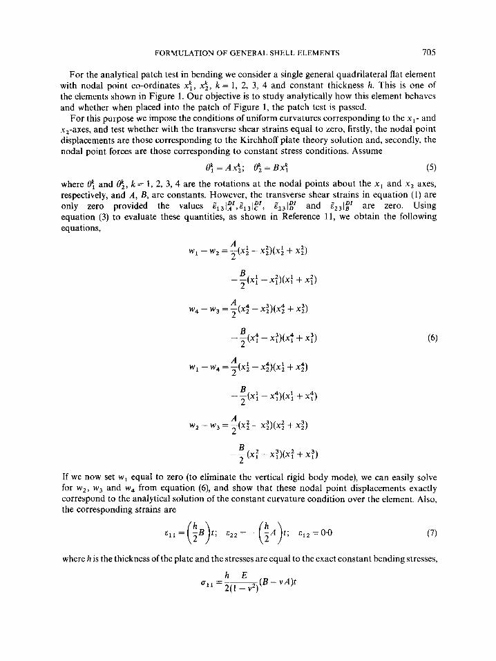
For the analytical patch test in bending we consider a single general quadrilateral flat element with nodal point co-ordinates xt , xk,, k = 1, 2, 3, 4 and constant thickness h. This is one of the elements shown in Figure 1. Our objective is to study analytically how this element behaves and whether when placed into the patch of Figure 1, the patch test is passed.

For this purpose we impose the conditions of uniform curvatures corresponding to the x l - and x,-axes, and test whether with the transverse shear strains equal to zero, firstly, the nodal point displacements are those corresponding to the Kirchhoff plate theory solution and, secondly, the nodal point forces are those corresponding to constant stress conditions. Assume

@=AX:; ek,=Bx: ( 5 )

where @ and 6, k = 1, 2, 3, 4 are the rotations at the nodal points about the x1 and x2 axes, respectively, and A, B, are constants. However, the transverse shear strains in equation (1) are only zero provided the values El3l~',El31~', Ez3Ig' and E231f are zero. Using equation (3) to evaluate these quantities, as shown in Reference 11, we obtain the following equations,

A 2

w 1 - w2 =-(xi - .:)(xi + x:)

B 2

- -(x; - x:)(x: + x:)

A 2

w4 - w3 = -(x; - x:)(x: + x:) B 2

- -(x; - x:)(x: + x?)

A 2

w1 - w4 = -(xi - xf)(x; + Xt)

B - -(xt 2 - x;)(x: + x:) A 2 w2 - w3 =-(xi - .:)(xi + x;)

B 2

- -(x; - x:)(x: + x:)

If we now set w1 equal to zero (to eliminate the vertical rigid body mode), we can easily solve for w2, w3 and w4 from equation (6), and show that these nodal point displacements exactly correspond to the analytical solution of the constant curvature condition over the element. Also, the corresponding strains are

E~~ = (;B)t; E~~ = - (;A)t; c12 = 0.0 (7)

where his the thickness of the plate and the stresses are equal to the exact constant bending stresses,

( B - vA)t 0 1 1 =-- h E 2(1 - v2)

706

I

M E S H w C FEM/& M;I:/tt%

4 x4 0.879 0.873 0.852

8 x 8 0.871 0.928 0.922

1 6 X 16 0.933 0.961 0.9 19

32 X 32 0.985 0.989 0.990

K. J. BATHE AND E. N. DVORKIN

h E 022 = - - ( - A + vB) t

2(1 - v’)

012=013=023=033 ~ 0 . 0

Hence-using also that the in-layer strains are those of a compatible plane stress element-the correct nodal point forces for the deformation considered are calculated and the patch test is passed.

3.3 Some demonstrative sample solutions

We have discussed some solution experiences with our 4 - n d e element already in References 6 and 11; however, we want to add here a few further results. These add to demonstrate the performance of the element in the analysis of complex problems. We refer to our element as the MITC4 element (an abbreviation for mixed interpolation of tensorial components with 4 nodes).

As pointed out already, our element passes the patch tests of Figure 1 exactly.

Y

b 4 X 4 M E S H

SIMPLY SUPPORTED EDGES

E=30* lo6

V =0.3

b = l

thicknerr=0.01 uniform p r r r i u r e p=l

BOUNDARY CONDITION u=O

ON FOUR EDGES

FORMULATION OF GENERAL SHELL ELEMENTS

-

MESH

2 x 2 0 984 0 717 0 6 0 2

4 x 4 0 994 0 935 0 878

707

2 x 2 MESH

E = 1 . 1 0 ~

V = 0 . 3

L 1100

a = 2

thickness ( h ) = I

P = 5

max - rbendinQ

b - 3 P - h2

Figure 4. Analysis of a plate with a hole under transverse twisting using the MITC4 element. The stresses are directly calculated at point A


u: TIP LONGITUDINAL DISPLACEMENT

w: TIP TRANSVERSE DISPLACEMENT

d: TIP ROTATION

TWO 4-NODE ELEMENT MODEL

THREE 4 - N O D E ELEMENT MODEL

L = I 2 € = I 8 0 0

b = l u = o

h = l

- ANALYT. SOLN. '.I W - L

4 21r

M L 2xEr

f 0.8

- 0.6

- 4 27r 0.4

0.2

0.1 0.2 0.3

ML 27rE I

Figure 5. Large displacement/rotation analysis of a cantilever using the MITC4 element


E = 21,000 v-0

ET= 0

(Jyz4.2

L =15,200

R = 7,600 RIGID USED TO REPRESENT AREA ABCD c$= 400

thickness576 x lo3

0 Krdkelond [I71 1 / = -MlTC4

2 t t 4 POINT GAUSS INTEGRATION THROUGH ELEMENT THICKNESS

50 100 150 200

W B

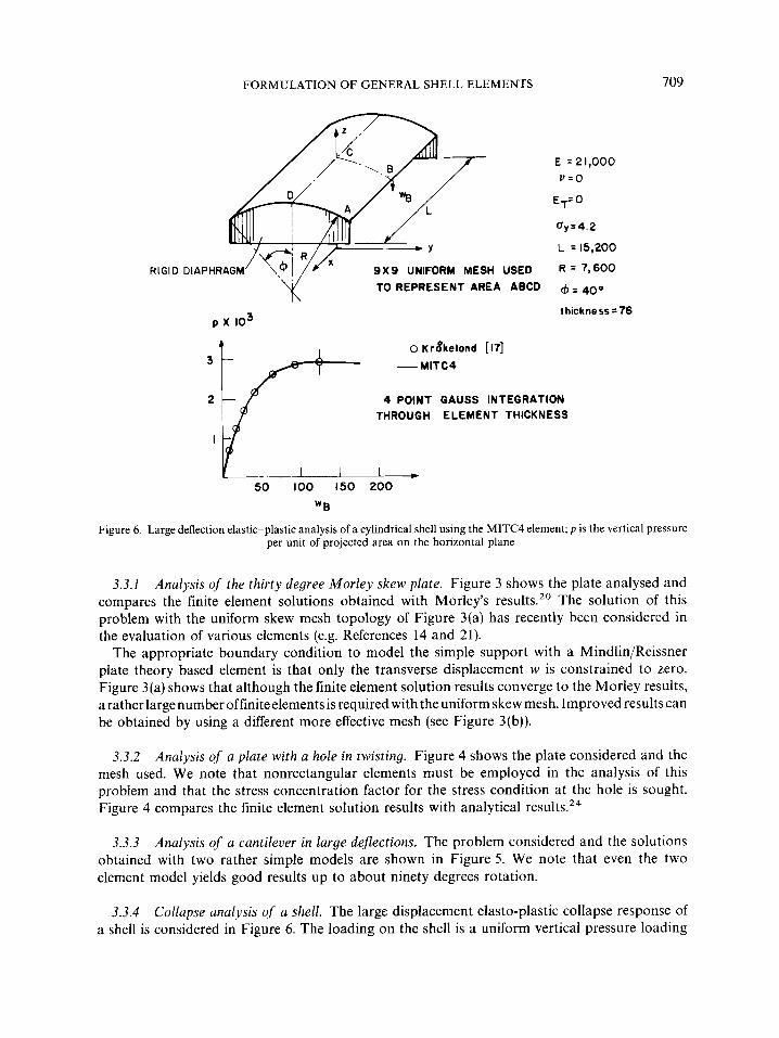
Figure 6 . Large deflection elastic-plastic analysis of a cylindrical shell using the MITC4 element; p is the vertical pressure per unit of projected area on the horizontal plane

3.3.1 Analysis of the thirty degree Morley skew plate. Figure 3 shows the plate analysed and compares the finite element solutions obtained with Morley’s results.” The solution of this problem with the uniform skew mesh topology of Figure 3(a) has recently been considered in the evaluation of various elements (e.g. References 14 and 21).

The appropriate boundary condition to model the simple support with a Mindlin/Reissner plate theory based element is that only the transverse displacement w is constrained to zero. Figure 3(a) shows that although the finite element solution results converge to the Morley results, a rather largenumber offiniteelementsis required with theuniform skew mesh. Improved resultscan be obtained by using a different more effective mesh (see Figure 3(b)).

3.3.2 Analysis of a plate with a hole in twisting. Figure 4 shows the plate considered and the mesh used. We note that nonrectangular elements must be employed in the analysis of this problem and that the stress concentration factor for the stress condition at the hole is sought. Figure 4 compares the finite element solution results with analytical results.24

3.3.3 Analysis of a cantilever in large deflections. The problem considered and the solutions obtained with two rather simple models are shown in Figure 5. We note that even the two element model yields good results up to about ninety degrees rotation.

3.3.4 Collapse analysis of a shell. The large displacement elasto-plastic collapse response of a shell is considered in Figure 6. The loading on the shell is a uniform vertical pressure loading


per unit of projected area on the horizontal plane. The solution is compared with the response predicted by Krikeland,” who solved for the response up to wB = 125. To traverse the point of maximum load carrying capacity we used in our solution the automatic load incrementation algorithm of Reference 7.

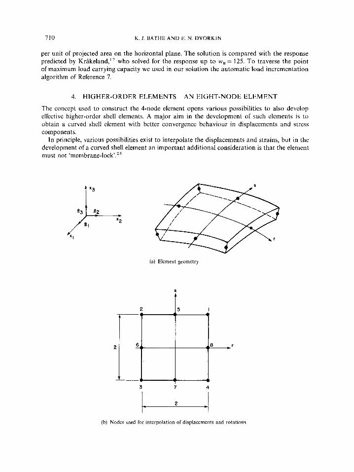
4. HIGHER-ORDER ELEMENTS-AN EIGHT-NODE ELEMENT

The concept used to construct the 4-node element opens various possibilities to also develop effective higher-order shell elements. A major aim in the development of such elements is to obtain a curved shell element with better convergence behaviour in displacements and stress components.

In principle, various possibilities exist to interpolate the displacements and strains, but in the development of a curved shell element an important additional consideration is that the element must not ‘membrane-lo~k‘.~~

(a) Element geometry

b

t

3 7 4

(b) Nodes used for interpolation of displacements and rotations

t

t

+---I+ 0 0-

2 I

(c) Points used for interpolation of in-layer strains

S b

2 I n -

S

(d) Points used for interpolation of transverse shear strain Fr,,g'gf

t

Points used for interpolation of transverse shear strain &gag'

Figure 7. Eight-node shell element


In studying various possible interpolations analytically and numerically we identified that the 8-node element described below offers much promise (see Figure 7). At each nodal point, the same kinematic description using director vectors and five degrees of freedom as for our 4-node element (and the 16-node element3) is used. Hence, the displacements are interpolated as usual for the degenerate isoparametric shell elements3 with the displacement interpolation functions hi,

h , = $ ( l +r)( l +s) -&+h*) ; h ,= i ( l - Y ) ( l + S ) - + ( h 5 + h 6 )

h, =+(1 -r2)(1 +s); h, = $ ( 1 - s z ) ( l - r ) (9)

h - -1 4(t - r)(l - s) - )(h, + h7); h, = +(I + r ) ( l - s) - + ( A 8 + h7)

h, = i ( 1 - r2)(1 - s); h, =$(l - s2)(1 + Y)

To avoid membrane and shear locking we interpolate the in-layer strains and the transverse shear strains independently-with appropriately selected interpolations-and tie the coefficients in these interpolations to the strain components evaluated directly from the displacement field. The in-layer strain interpolation yields the membrane and bending action of the element, and the transverse shear strain interpolation gives the transverse shear action. To obtain a general shell element, we interpolate the strain tensor expressed in terms of covariant components and contravariant base vectors.

In the following discussion we consider the element strain tensor at any time during the response history. However, for the incremental formulation we refer to References 3 and 11, and therefore we do not include the left superscript denoting time (e.g. henceforth g, = 'gr) . Also, we use the notation g, = g , , g, = g, and g, = g,.

The strain tensor at any point in the element is,

E = zrrgrgr + zssgsgs + Ers(g'g" + g",) I .............................................. I

in-layer strains

+ M g r g t + g'g') + zs,(g"gg' + g r g 7 I ------- ------ ........................ I I I

transverse shear strains

where g', g', g' are the contravariant base vectors corresponding to the covariant base vectors g,, g,, gt , which are evaluated as given in equation (4).

The appropriate interpolation of the in-layer strains and of the transverse shear strains to satisfy our shell element requirements as closely as possible is the key aspect of our element formulation.

4.1 In-layer strain interpolation

To avoid membrane locking and have no spurious zero energy modes, we use the following in-layer strain interpolation, see Figure 7(c),

8

& = c hfS&li ( 1 1) i = 1

where the hfs are obtained from the hi in equation (9) by replacing the variable I with rla, and the variable s with sla, a = I/$.

Also, we have for i = 1, 2, 3 and 4,


where

Equation (11) corresponds to a mixed interpolation of the tensor components such that the membrane patch test is passed (for straight-sided elements) and, in non-flat elements, membrane locking is avoided.

4.2 Transverse shear strain interpolation

The transverse shear strain interpolation is selected to avoid shear locking and, as for the in-layer strain interpolation, no spurious zero energy mode must be introduced. We use the following interpolation for Er,grg' (see Figure 7(d)),

where

714 K. J. BATHE A N D E. N. DVORKIN

where a = l/$. We note that in equation (19) we have replaced Err[:' by the mean of the components at points R A and RB.

Similarly, we use the following interpolation for Esrgsg' (see Figure 7(e)), 4

s f DI s r DI &gsgg' = C hYEsrg g Ii hYC*(EsrIC + krIsD)Ig g I 5 i = 1

where

h z T = a ( l -I) 1 +- - l h S T ( r) 4 5

( r) 4 5

( r) 4 5

hS,T=,( l - , ) I - - -lhST

hiT =$(I + r ) 1 -- - LhsT

h<T = (1 - ($')(1- 1')

where a = 1/J3.

4.3 Some remarks regarding the 8-node element

With the interpolation functions available, the implementation of the element for linear and nonlinear analysis follows the procedures given in References 3 and 1 1. For geometric nonlinear analysis we have implemented the total Lagrangian formulation (allowing for very large displacements and rotations but assuming small strain conditions).

The Remarks 1 to 5 given for our 4-node element in Section 3.1 are also applicable to this 8-node element. However, for the mid-surface numerical integration we now use 3 x 3 Gauss integration.

4.4 Some demonstrative sample solutions

As mentioned in Section 2.2, we tested our element on the patch tests of Figure 1. These patch tests-using elements with straight sides-are all passed exactly. However, relatively small errors in displacements and stresses arise when the element sides are curved, or when the mid-side nodes are not placed at their mid-side physical locations.

The results obtained in the example solutions given below demonstrate the solution characteristics of the element. We refer to our new element as element MITC8.

4.4.1 Analysis of a plate with a hole in plane stress. To illustrate the difference in stress prediction between our new 8-node element and the usual isoparametric 8-node element in plane stress, we give the results obtained in the analysis of the plate shown in Figure 8. A relatively coarse mesh is used in the analysis.

For the stress calculations the strains have in both analyses been obtained from the strain-displacement matrices evaluated directly at the points C and D. Hence, no stress extrapolation or stress smoothing has been used. Figure 8 shows that the 8-node isoparametric

FORMULATION OF GENERAL SHELL ELEMENTS

FEM ANALYT. CALCULATED 3 2 /.Zt

AT POINT ISOP. ELEMENT M , T C e 3 X 3 X 2 INTEGRN. :

715

C

0

L = 56 E = 7 . 104

b = 20 V = 0.25 d =I0 p = 25 h (thickness ) = I

0.953 0.943

I. 013 I. 038

MESH USED

Figure 8. Analysis of a plate with a hole in plane stress using the MITC8 element. The stresses are directly calculated at points C and D

element yields a slightly more accurate solution. This is not a surprise, because the element passes the membrane patch test even for curved element sides.

4.4.2 Analysis of a curved cantilever. The analysis of the curved cantilever subjected to a bending moment shown in Figure 9 illustrates the predictive capability of our 8-node element when used as a curved element in a problem that would display shear and membrane locking.8 Figure 9 shows that excellent results are obtained with our element.

716 K. J . BATHE AND E. N. DVORKIN

L.2

0

thic

knel

r 0

.02

E =2

.1. I

06

Y

=0

.3

MES

H

IX I

2x

2

3x

3

E

2x

2 M

ES

H

UN

IFO

RM

PR

ESSU

RE

CO

NC

ENTR

ATE

D L

OA

D

0.9

93

1.0

03

1.00

0 0.9

98

1.00

0 0.9

99

BO

UN

DA

RY

CO

ND

ITIO

NS

-SIM

PLY

SUPP

OR

TED

ED

QE

w.0

-CLA

MP

ED

E

DO

E

w.0

et 8

0

1.24

0 1.1

16

1.0

06

1.00

0

1.00

5 1.

001

E I P I rTt7

m.

C

e

FEM

L=

1.00

1 .A

NALY

1.

C

-P

(a)

Res

ults

usi

ng u

ndis

tort

ed e

lem

ents

(b

) R

esul

ts u

sing

dis

tort

ed e

lem

ents

; cas

e of s

impl

y-su

ppor

ted

plat

e an

d un

iform

pre

ssur

e. T

he e

lem

ent d

isto

rtio

ns a

re s

how

n to

sca

le

Figu

re 1

0. A

naly

sis o

f sq

uare

pla

te u

sing

the

MIT

CI

elem

ent.

The

ana

lytic

al so

lutio

n us

ed a

s re

fere

nce

is th

e K

irchh

off

plat

e th

eory

sol

utio

nz7

r

71 8 K. J. BATHE A N D E. N . DVORKIN


R =300

L = 600 /

specific weight = 0.20833

RlG lD DIAPHRAGM

FEM I I MESH FOR AREA A B C D 1 WP

ANALYTICAL SOLUTION ~ ~ ~ 3 . 6 [12]

(DEEP SHELL THEORY)

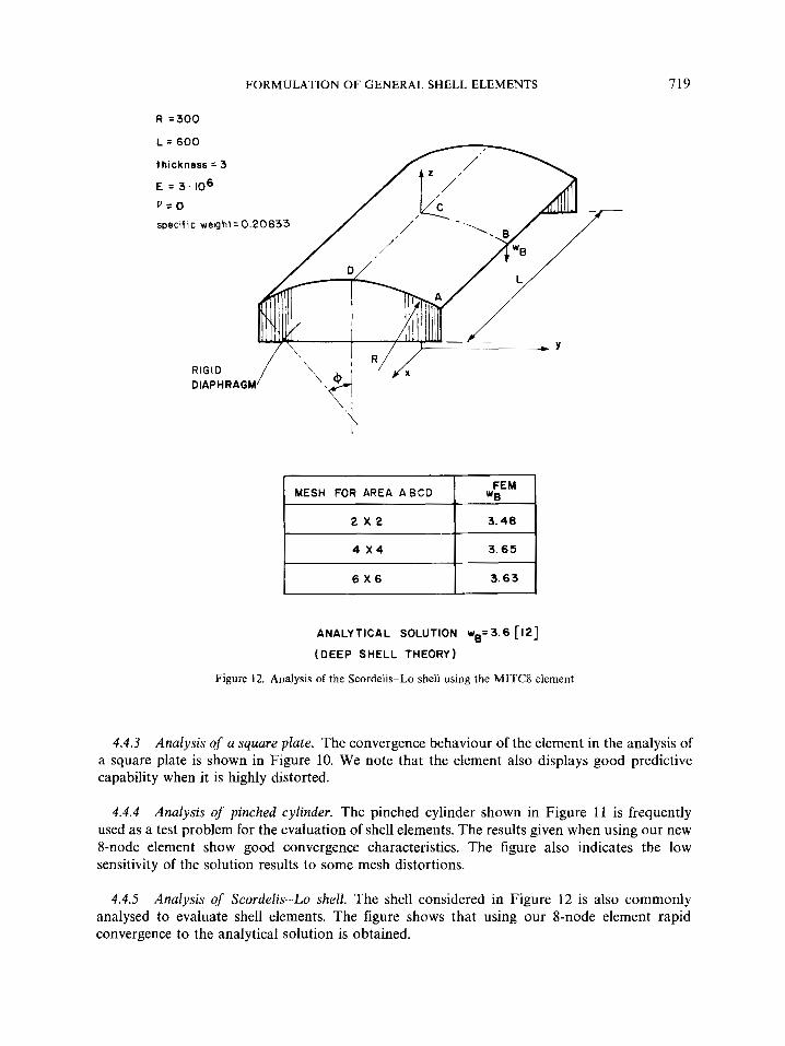
Figure 12. Analysis of the Scordelis-Lo shell using the MITC8 element

4.4.3 Analysis of a square plate, The convergence behaviour of the element in the analysis of a square plate is shown in Figure 10. We note that the element also displays good predictive capability when it is highly distorted.

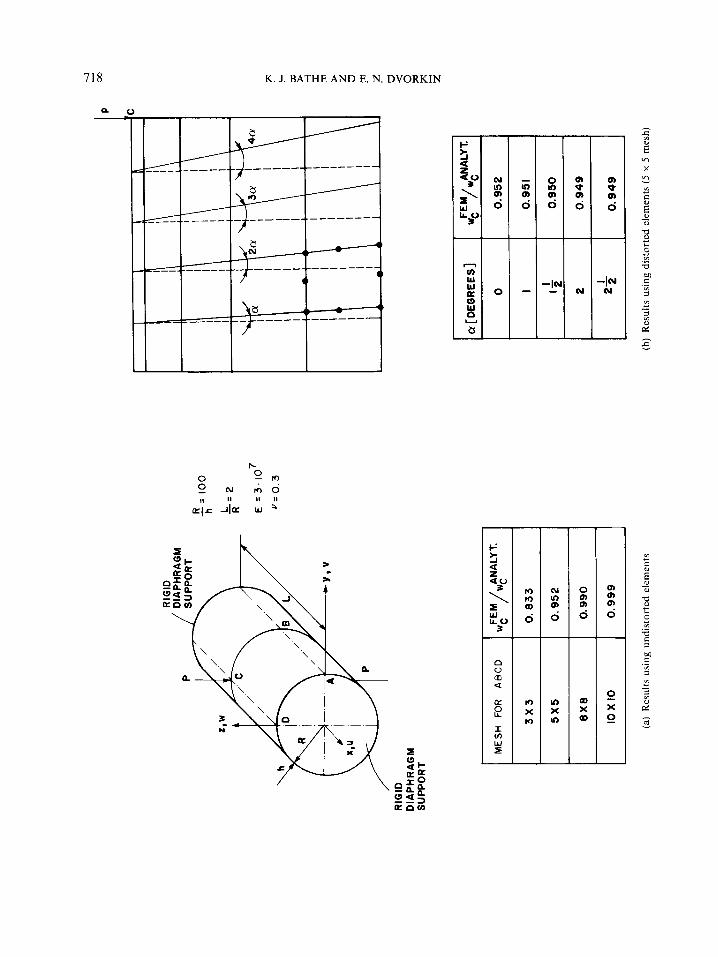
4.4.4 Analysis of pinched cylinder. The pinched cylinder shown in Figure 11 is frequently used as a test problem for the evaluation of shell elements. The results given when using our new &node element show good convergence characteristics. The figure also indicates the low sensitivity of the solution results to some mesh distortions.

4.4.5 Analysis of Scordelis-Lo shell. The shell considered in Figure 12 is also commonly analysed to evaluate shell elements. The figure shows that using our 8-node element rapid convergence to the analytical solution is obtained.


E = leoo ONE 8-NODE ELEMENT MODEL L = 12

b = I v: 0

h = I

t

0.8

' -% L

L I I

~

0. I 0.2 0.3

- ANALYT. SOLN.

MITC8

STANDARD - ISOPARAMETRIC ELEMENT ( 3 X 3 X 2 GAUSS INTEGRN)

----

- 4

Figure 13. Large displacernent/rotation analysis of a cantilever using the MITCR element

4.4.6 Anatysis of a cantifever in large dejections-use of 8-node element. The cantilever already considered in Figure 5 has also been analysed using our new 8-node element. Figure 13 shows the simple one element model and the solution results obtained. We observe that even using only one element to model the cantilever excellent results are obtained for up to about ninety degrees rotations.

The standard isoparametric 8-node element with 'full' integration, which matches the exact result in linear analysis, locks in the large displacement solution.

5. CONCLUDING REMARKS

The objective in this paper was to discuss a general approach using mixed interpolation of tensorial components towards formulating widely applicable shell elements, and to present a new 8-node element based on this approach.

FORMULATION OF GENERAL SHELL ELEMENTS 72 1

A general shell element for linear and nonlinear analysis should be developed by concentrating directly on the requirements of general shell analysis. This element can then be degenerated to special shell situations, such as the linear analysis of plates.

The approach of shell element formulation presented in this paper shows good promise in that aim: the four-node element is effective and reliable and can be applied to very complex shell analyses and the eight-node element is also quite attractive. However, this element should be further tested and analysed, theoretically and numerically, which may well lead to refinements in its formulation. Specifically, the aim might be to improve the element so that it satisfies the patch tests for ‘any’ distorted element shapes. Such improvement should result in better predictive capabilities in general. The construction of an effective 9-node element, other higher-order shell elements and transition elements should also be possible.

Considering the formulation approach and the 8-node element described in the paper, the element construction is based on insight into element behaviour and the use of the patch tests. It would be valuable to place the approach on a more structured mathematical foundation which gives analytically general conditions of stability and convergence. The patch test is an excellent tool in this regard, but perhaps even more powerful analytical conditions and tests can be identified.

ACKNOWLEDGEMENT

We would like to thank J. Dong of ADINA Engineering, Inc. for his help in some of the example analyses.

REFERENCES

1. S. Ahmad, B. M. Irons and 0. C. Zienkiewicz, ‘Analysis of thick and thin shell structures by curved finite elements’, f n t . j . numer. methods eny., 2, 419-451 (1970).

2. S. Atluri and T. H. H. Pian, ‘Theoretical formulation of finite-element methods in linear-elastic analysis of general shells’, J . Struct. Mech., 1, 1-41 (1972).

3. K. J. Bathe, Finite Element Procedures in Engineering Analysis, Prentice-Hall, Englewood Cliffs, New Jersey, 1982. 4. K. J. Bathe and S. Bolourchi, ‘A geometric and material nonlinear plate and shell element’, J . Com. Struct. 11, 23-48

( 1 979). 5. K. J. Bathe and F. Brezzi, ‘On the convergence of a four-node plate bending element based on Mindlin/Reissner plate

theory and a mixed interpolation’, Proc. Conf. on Mathematics of Finite Elements and Applications V, Brunel University, England, 1984.

6. K. J. Bathe and E. N. Dvorkin, ‘A four-node plate bending element based on Mindlin/Reissner plate theory and a mixed interpolation’, f n t . j . numer. methods eng., 21, 367-383 (1985).

7. K. J. Bathe and E. N. Dvorkin, ‘On the automatic solution of nonlinear finite element equations’, J . Comp. Struct., 17, 871-879 (1983).

8. K. J. Bathe, E. N. Dvorkin and L. W. Ho, ‘Our discrete-Kirchhoff and isoparametric shell elements for nonlinear analysis-an assessment’, J. Comp. Struct., 16, 89-98 (1983).

9. K. J. Bathe and L. W. Ho, ‘Some results in the analysis of thin shell structures’, in Nonlinear Finite Elemtnf Anulysis in Structural Mechanics (W. Wunderlich et al. Eds.), Springer-Verlag, Berlin, 198 1.

10. M. A. Crisfield, ‘A quadratic Mindlin element using shear constraints’, J . Comp. Struct., 18, 833-852 (1984). I I. E. N. Dvorkin and K. J. Bathe, ‘A continuum mechanics based four-node shell element for general nonlinear analysis’,

12. K. Forsberg and R. Hartung, ‘An evaluation of finite difference and finite element techniques for analysis of general

13. W. Fliigge, Stresses in Shells, 2nd edn, Springer-Verlag, Berlin, 1973. 14. H. C. Huang and E. Hinton, ‘A nine node Lagrangian Mindlin plate element with enhanced shear interpolation’, Eng.

15. T. J . R. Hughes and T. E. Tezduyar, ‘Finite elements based upon Mindlin plate theory with particular reference to the

16. B. Irons and S. Ahmad, Techniques qf Finite Elements, Ellis Horwood, Chichester, U.K., (1980). 17. B. Krgkeland, ‘Nonlinear analysis of shells using degenerate isoparametric elements’, in Finife Elements in Nonlinetrr

Mechanics, Vol. 1 (P. G. Bergan et al. Eds.), Tapir Publishers (Norwegian Inst. of Tech. Trondheim, Norway), 1978.

Eng. Comput., 1, 77-88 (1984).

shells’, Symp. on High Speed Computing of Elastic Structures, I.U.T.A.M., Liege, 1970.

Comput., 1, 369-379 (1984).

four-node bilinear isoparametric element’, ASME, J . Appl. Mech.. 46, 587-596 (1 98 1).


18. G. M. Lindberg, M. D. Olson and G. R. Cowper, ‘New developmentsin the finite element analysis ofshells’, Q. Bull. Diu.

19. R. H. MacNeal, ‘Derivation ofelement stiffness matrices by assumed strain distributions’, J . Nucl. Eny. Design. 70,3-12

20. L. S . D. Morley, Skew Plates and Structures, Pergamon Press, Oxford, 1963. 21. K. C. Park and G. M. Stanley, ‘A curved Co shell element based on assumed natural-coordinate strains’, Report N o .

22. T. H. H. Pian and P. Tong, ‘Basis of finite element methods for solid continua’, Int. j . numer. methods eng., 1.3-28 (1969). 23. E. Ramm, ‘A plate/shell element for large deflections and rotations’, in Formulations and Computational Algorithms in

24. E. Reissner, ‘On the transverse twisting of shallow spherical ring caps’, ASME, J . Appl. Mech., 47, 101-105 (1980). 25. H. Stolarski and T. Belytschko, ‘Membrane locking and reduced integration for curved elements’, ASME, J . Appl.

26. G. Strang and G. J. Fix, An Analysis of the Finite Element Method, Prentice-Hall, Englewood Cliffs, New Jersey, 1973. 27. S. P. Timoshenko and S. Woinowsky-Krieger, Theory of Plates and Shells, 2nd edn, McGraw-Hill, New York, 1959. 28. K. Washizu, Variational Methods in Elasticity & Plasticity, 3rd edn, Pergamon Press, London, 1982. 29. G. Wempner, D. Talaslidis and C.-M. Hwang, ‘A simple and efficient approximation of shells via finite quadrilateral

elements’, ASME, J . Appl. Mech., 49, 115-120 (1982). 30. W. WunderIich, ‘Incremental formulations for geometrically-nonlinear problems’, in Formulations and Computationaf

Algorithms in Finite Element Analysis (K. J. Bathe et al. Eds.), M.I.T. Press, 1977. 31. 0. C. Zienkiewicz, The Finite Element Method, 3rd edn, McGraw-Hill, London, 1977.

Mech. Eny. and Nat . Aeronaut. Establishment, National Research Council of Canada, Vol. 4, 1969.

(1982).

LMSC-F035235, Applied Mechs. Lab., Lockheed Palo Alto Research Lab. (1984).

Finite Element Analysis, (K. J. Bathe et al. Eds.), M.I.T. Press, 1977.

Mech., 49, 172-176 (1982).

a use of - web.mit.eduweb.mit.edu/kjb/www/publications_prior_to_1998/a_formulation_of... ·...

Documents