amplitude modulation using multipliers and envelope detector
TRANSCRIPT

1
A Project Based Lab Report On AMPLITUDE MODULATION USING MULTIPLIERS AND
ENVELOPE DETECTOR Submitted in partial fulfilment of the Requirements for the award of the Degree of Bachelor of Technology In Electronics & Communication Engineering By SK.JUNEZ RIYAZ (Id No-150040793) Under the guidance of Guide Name: Mr.YGSK Naidu Designation: Asst. Professor
Dept. of Electronics and Communication Engineering
K.L. UNIVERSITY Green fields,Vaddeswaram-522502, Guntur Dist. 2016-17

2
DEPARTMENT OF ELECTRONICS AND ENGINEERING
CERTIFICATE
This is to certify that this project based lab report entitled “AMPLITUDE MODULATION USING MULTIPLIERS AND ENVELOPE DETECTOR” is a bonafide work done by SK.JUNEZ RIYAZ (Id No-150040793) in partial fulfilment of the requirement for the award of degree in Bachelor of Technology in Electronics and Communication Engineering during the academic year 2016-2017.
I also declare that this project based lab report is of our own effort and it has not been submitted to any other university for the award of any degree.
Signature of the Project guide Signature of Course Coordinator
Head
Dep. Of ECE

3
ACKNOWLEDGMENT
My sincere thanks to in the Lab for their outstanding support throughout the project for the
successful completion of the work.
We express our gratitude to Dr. ASCS SASTRY, Head of the Department for Electronics and
Communication Engineering for providing us with adequate facilities, ways and means by
which we are able to complete this project based work.
We would like to place on record the deep sense of gratitude to the honourable Vice Chancellor,
K L University for providing the necessary facilities to carry the concluded project based work.
Last but not the least, we thank all Teaching and Non-Teaching Staff of our department and
especially my classmates and my friends for their support in the completion of our project based
work.
Place: KL University
SK.JUNEZ RIYAZ (Id No-150040793)
4
CONTENTS CONTENT Page No Abstract 5 Problem statement: 5 Chapter 1: Introduction 7 Chapter 2: Tasks Simulation Results 10 (a) Task1 10 (b) Task2: 12 (c) Task3: 15 (d) Task4: 18 Chapter 3: 22
Applications 22 Conclusions and future scope 23
References 23

5
Abstract
The project amplitude modulation using multipliers and envelope
detection is useful for communication purpose where the receptors
are far away from the emitter. Here at the emitting side we will
modulate the signal since it is weak to travel that much distance.
After receiving the signal at the receiver they will demodulate it.
Here in this project we are using envelope detector for the
demodulation purpose, so if we do frequency or phase modulation the
envelope would be a straight lines divided by some space. But if we
modulate the amplitude then we can recapture the signal very
easily using envelope detector.
Problem Statement
To generate amplitude modulation signals.
To design an envelope detection for given modulating signal or speech signal
Exposure to simulation on modulation/demodulation systems for Amplitude
Modulation using MATLAB for synthetic & real signals (such as speech).
A base band signal m(t) is used to generate Amplitude Modulated signal
j AM (t) = Ac[1+m(t)] cos(Wct) , where c(t) is a carrier signal c(t) = Ac cosWct as
shown in the Fig.1. The objective is to explore the theoretical concepts of AM signal by
modeling and simulation using Matlab and Simulink

6
Block diagram of Amplitude Modulation and Envelope Detection system.
Task1:
Consider a single tone modulating signal m(t) = cos860p t , and carrier signal with
frequency
of 9000 Hz .
1. Determine the expression for Amplitude Modulated signal in both time domain and
frequency domain.
2. Sketch the modulating signal m(t) and its spectrum.
3. Sketch the carrier signal c(t) and its spectrum.
4. Sketch the Amplitude Modulated signal ( ) AM j t and its spectrum.
5. Identify the USB, LSB and carrier spectra.
6. Determine the maximum and minimum amplitudes of the envelope.
7. Find the powers of USB, LSB, total sideband, carrier and modulated signals.
Task 2:
Assume that the demodulation process is envelope detection as shown in Figure.
The objective is to design an envelope detector in demodulation / reception of amplitude
modulated wave.
Task 3:
Repeat the above Tasks for multi tone signal
2cos1000 p t -sin1500p t +1.5cos2000p t
Task4:
Repeat above tasks for real speech signals.

7
Objectives
1) Understanding the basic theory of Modulation and Demodulation.
2) Implementing the Amplitude Modulation and Demodulation using low pass
filter in MAT LAB for different types of signals .
3)understanding the working of filter.
Modulation and Demodulation is to prevent the unwanted signals which are
not in the particular band of frequency and retrieve the original signal
(message signal) .In this project the modulation and demodulation of the
single tone message signal , multi tone message signals,recored voice,music
signals ,female and male voice are performed with the carrier wave of sine for
modulation and carrier wave of cosine for demodulation and after performing
this operations the demodulated signal is passed through the low pass filter in
order to get the desired out put i..e the signal in the particular range of
frequency
Chapter 1-Introdution The frequency range audible to human begins known as audible range is between 20 Hz
to 20kHz .The frequency of human voice and music signals lies between 200 Hz to
4000Hz.Signals in the audible range audible range are not transmitted directly for the
following reason
1)The wave length of audible signals is very long .To transmit such signals signals the
size of
antenna must be atleast one tenth of signal wave length.
For example: consider a 1500Hz signal .The wavelength of the signal is(3*10^8)/1500
The height of antenna should be atleast 0.2*10^5 meters which is not possible practically
2) The signals in the audible range are not transmitted directly for the following reasons.

8
3)The audio signals attenuate rapidly in the atmosphere.
4)The interference will occur if two are more audio signals are transmitted
simultaneously.
Because of the above reasons the audio signals signals are modulated before modulation
.Not only for audio signals it is also used for signals to be transmitted for longer
distances.
Modulation is of three types they are:
Amplitude Modulation (AM)
Frequency Modulation (FM)
Phase Modulation (PM)
Amplitude Modulation In amplitude modulaton the amplitude of carrier wave is transmitted or varied in
accordance with
the instantaneous val;ue of the signal to be transmitted (modulated signal) i..e the
amplitude of the
carreir wave is varied in accordance with the message signal amplitude its from peak to
peak.
The figure 1.1 describes the modulation

9
Figure1.1 The figure 1.2 clearly describes the Amplitude modulation. m(t) is the message signal c(t) is the carrier signal the message signal is multiplied with carrier signal and the s(t) is amplitude modulated signal where the amplitude of the carrier is varied in accordance with message signal.
Figure1.3
Figure 1.3 gives the block diagram about the amplitude modulation here message is multiplied with carrier signal And output is as shown in the figure 1.2
Modulated wave = Eq-1
Demodulation
Demodulation is getting the required signal or output from the modulated wave. In
demodulation

10
the modulated signal is multiplied with carrier wave in order to get original information .
The carrier wave may be cosine or sine.
After demodulation the signal is passed through the lowpass filter as shown in the figure
0.1 then
the original signal will be obtained.
Figure1.4
From the above figure it can be described that y(t) is modulated signal and cos(w_ct) is the carrier wave and the z(t) is the demodulated signal. And then its passes through the filter to get the signal of required frequency and reject the unwanted frequency . Filter :It is a frequency selector(it allows particukar band of frequency to pass and the particular band of frequency to get rejected
Chapter 2 TASKS ,SIMULATION,RESULTS AND DISCUSSION Task1: Consider a single tone modulating signal m(t) = cos860p t , and carrier signal with frequency of 9000 Hz Code: fs=4000; N=5000; Ts=1/fs; t=(0:Ts:(N*Ts)-Ts); a=cos(860*pi*t); b=cos(2*pi*9000*t); k=a.*b; m=k+b; [v,A]=T2F(t,a); [w,B]=T2F(t,b); [f,M]=T2F(t,m);
11
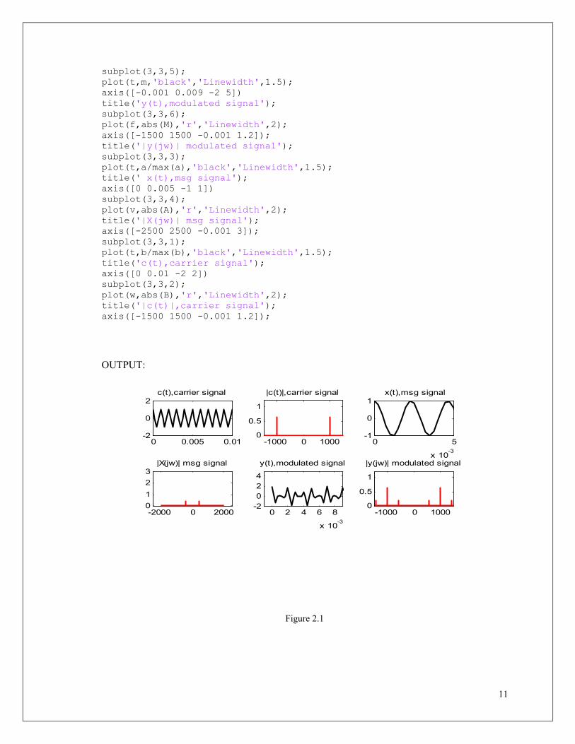
subplot(3,3,5); plot(t,m,'black','Linewidth',1.5); axis([-0.001 0.009 -2 5]) title('y(t),modulated signal'); subplot(3,3,6); plot(f,abs(M),'r','Linewidth',2); axis([-1500 1500 -0.001 1.2]); title('|y(jw)| modulated signal'); subplot(3,3,3); plot(t,a/max(a),'black','Linewidth',1.5); title(' x(t),msg signal'); axis([0 0.005 -1 1]) subplot(3,3,4); plot(v,abs(A),'r','Linewidth',2); title('|X(jw)| msg signal'); axis([-2500 2500 -0.001 3]); subplot(3,3,1); plot(t,b/max(b),'black','Linewidth',1.5); title('c(t),carrier signal'); axis([0 0.01 -2 2]) subplot(3,3,2); plot(w,abs(B),'r','Linewidth',2); title('|c(t)|,carrier signal'); axis([-1500 1500 -0.001 1.2]);
OUTPUT:
Figure 2.1
0 2 4 6 8
x 10-3
-2024
y(t),modulated signal
-1000 0 10000
0.5
1
|y(jw)| modulated signal
0 5
x 10-3
-1
0
1 x(t),msg signal
-2000 0 20000
1
2
3|X(jw)| msg signal
0 0.005 0.01-2
0
2c(t),carrier signal
-1000 0 10000
0.5
1
|c(t)|,carrier signal

12
Task2
Assume that the demodulation process is envelope detection as shown in Figure.
The objective is to design an envelope detector in demodulation / reception of amplitude modulated wave
Code: % AM demodulation using Envelope detection clear all; close all; clc; % Generation of AM single tone fs=6000; N=5000; Ts=1/fs; t=(0:Ts:(N*Ts)-Ts); a=cos(860*pi*t); b=cos(2*pi*9000*t); k=a.*b; m=k+b; [v,A]=T2F(t,a); [w,B]=T2F(t,b); [f,M]=T2F(t,m); subplot(3,3,5); plot(t,m,'black','Linewidth',1.5); axis([-0.001 0.009 -2 5]) title('y(t),modulated signal'); subplot(3,3,6); plot(f,abs(M),'r','Linewidth',2); axis([-3000 3000 -0.001 1.2]); title('|y(jw)| modulated signal'); subplot(3,3,3); plot(t,a,'black','Linewidth',1.5); title(' x(t),msg signal'); axis([0 0.005 -1 1]) subplot(3,3,4); plot(v,abs(A),'r','Linewidth',2); title('|X(jw)| msg signal'); axis([-3000 3000 -0.001 1]); subplot(3,3,1); plot(t,b,'black','Linewidth',1.5); title('c(t),carrier signal'); axis([0 0.01 -2 2]) subplot(3,3,2); plot(w,abs(B),'r','Linewidth',2); title('|c(t)|,carrier signal'); axis([-3200 3200 -0.02 1.2]); figure(); plot(t,a,'black','Linewidth',1.5);grid on title(' x(t),msg signal'); axis([0 0.005 -1 1]) legend('Message Signal'); % %%% --------- Envelope Detector ---------------------- sf = abs(m); % Halfwave Rectifier % Spectrum of rectified signal fh = (-N/2:1:N/2-1)*fs/N; Sf = (2/N)*fftshift(fft(sf));

13
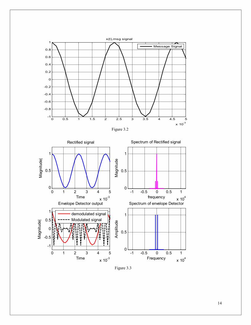
[a,b]=butter(9,0.172) ; % LPF tranfer function env = filtfilt(a,b,sf); % Low pass filtering the rectified signal env = env-mean(env); % Removing the DC % Spectrum of envelope detected signal fenv = (-N/2:1:N/2-1)*fs/N; Senv = (2/N)*fftshift(fft(env)); figure(); subplot(2,2,1); plot(t,abs(sf)/max(abs(sf)),'b','Linewidth',2);grid on; axis([0 0.005 -0.02 1.2]); xlabel('Time'); ylabel('Magnitude|'); title('Rectified signal'); subplot(2,2,2); plot(fh,real(Sf)/max(real(Sf)),'m','Linewidth',2);axis([-12000 12000 -0.0012 1.2]); xlabel('frequency'); ylabel('Magnitude'); title('Spectrum of Rectified signal '); grid on subplot(2,2,3); plot(t,env, 'r', 'LineWidth',1.5);axis([0 0.005 -1.2 1.2]);hold on plot(t,m/max(m), '--k', 'LineWidth',1.5);axis([0 0.005 -1.2 1.2]); xlabel('Time'); ylabel('Magnitude|'); title('Envelope Detector output'); grid on; legend('demodulated signal','Modulated signal'); subplot(2,2,4); plot(fenv,abs(Senv)/max(abs(Senv)), 'b', 'LineWidth',1.5);axis([-12000 12000 -0.0012 1.2]); xlabel('Frequency');ylabel('Amplitude');title('Spectrum of envelope Detector'); grid on; figure(); plot(t,env, 'r', 'LineWidth',1.5);axis([0 0.02 -1.2 1.2]); xlabel('Time'); ylabel('Magnitude|'); title('Envelope Detector output'); grid on; legend('Demodulated Signal'); Output
Figure 3.1
0 2 4 6 8
x 10-3
-2
024
y(t),modulated signal
-2000 0 20000
0.5
1
|y(jw)| modulated signal
0 5
x 10-3
-1
0
1 x(t),msg signal
-2000 0 20000
0.5
1|X(jw)| msg signal
0 0.005 0.01-2
0
2c(t),carrier signal
-2000 0 20000
0.5
1
|c(t)|,carrier signal
14
Figure 3.2
Figure 3.3
0 0.5 1 1.5 2 2.5 3 3.5 4 4.5 5
x 10-3
-1
-0.8
-0.6
-0.4
-0.2
0
0.2
0.4
0.6
0.8
1 x(t),msg signal
Message Signal
0 1 2 3 4 5
x 10-3
0
0.5
1
Time
Mag
nitu
de|
Rectified signal
-1 -0.5 0 0.5 1
x 104
0
0.5
1
frequency
Mag
nitu
de
Spectrum of Rectified signal
0 1 2 3 4 5
x 10-3
-1
-0.5
0
0.5
1
Time
Mag
nitu
de|
Envelope Detector output
demodulated signal
Modulated signal
-1 -0.5 0 0.5 1
x 104
0
0.5
1
Frequency
Am
plitu
de
Spectrum of envelope Detector
15
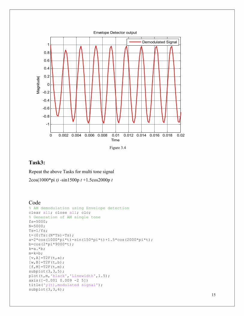
Figure 3.4
Task3:
Repeat the above Tasks for multi tone signal
2cos(1000*pi t) -sin1500p t +1.5cos2000p t
Code % AM demodulation using Envelope detection clear all; close all; clc; % Generation of AM single tone fs=5000; N=5000; Ts=1/fs; t=(0:Ts:(N*Ts)-Ts); a=2*cos(1000*pi*t)-sin(150*pi*t)+1.5*cos(2000*pi*t); b=cos(2*pi*9000*t); k=a.*b; m=k+b; [v,A]=T2F(t,a); [w,B]=T2F(t,b); [f,M]=T2F(t,m); subplot(3,3,5); plot(t,m,'black','Linewidth',1.5); axis([-0.001 0.009 -2 5]) title('y(t),modulated signal'); subplot(3,3,6);
0 0.002 0.004 0.006 0.008 0.01 0.012 0.014 0.016 0.018 0.02
-1
-0.8
-0.6
-0.4
-0.2
0
0.2
0.4
0.6
0.8
1
Time
Mag
nitu
de|
Envelope Detector output
Demodulated Signal

16
plot(f,abs(M),'r','Linewidth',2); axis([-1500 1500 -0.001 1.2]); title('|y(jw)| modulated signal'); subplot(3,3,3); plot(t,a/max(a),'black','Linewidth',1.5); title(' x(t),msg signal'); axis([0 0.005 -1 1]) subplot(3,3,4); plot(v,abs(A),'r','Linewidth',2); title('|X(jw)| msg signal'); axis([-2500 2500 -0.001 3]); subplot(3,3,1); plot(t,b/max(b),'black','Linewidth',1.5); title('c(t),carrier signal'); axis([0 0.01 -2 2]) subplot(3,3,2); plot(w,abs(B),'r','Linewidth',2); title('|c(t)|,carrier signal'); axis([-1500 1500 -0.001 1.2]); figure(); plot(t,a/max(a),'black','Linewidth',1.5);grid on title(' x(t),msg signal'); axis([0 0.005 -1 1]) legend('Message Signal'); % %%% --------- Envelope Detector ---------------------- sf = abs(m); % Halfwave Rectifier % Spectrum of rectified signal fh = (-N/2:1:N/2-1)*fs/N; Sf = (2/N)*fftshift(fft(sf)); [a,b]=butter(9,0.8) ; % LPF tranfer function env = filtfilt(a,b,sf); % Low pass filtering the rectified signal env = env-mean(env); % Removing the DC % Spectrum of envelope detected signal fenv = (-N/2:1:N/2-1)*fs/N; Senv = (2/N)*fftshift(fft(env)); figure(); subplot(2,2,1); plot(t,abs(sf)/max(abs(sf)),'b','Linewidth',2);grid on; axis([0 0.005 -0.02 1.2]); xlabel('Time'); ylabel('Magnitude|'); title('Rectified signal'); subplot(2,2,2); plot(fh,real(Sf)/max(real(Sf)),'m','Linewidth',2);axis([-12000 12000 -0.0012 1.2]); xlabel('frequency'); ylabel('Magnitude'); title('Spectrum of Rectified signal '); grid on subplot(2,2,3); plot(t,env/max(env), 'r', 'LineWidth',1.5);axis([0 0.005 -1.2 1.2]);hold on plot(t,m/max(m), '--k', 'LineWidth',1.5);axis([0 0.005 -1.2 1.2]); xlabel('Time'); ylabel('Magnitude|'); title('Envelope Detector output'); grid on; legend('demodulated signal','Modulated signal'); subplot(2,2,4); plot(fenv,abs(Senv)/max(abs(Senv)), 'b', 'LineWidth',1.5);axis([-12000 12000 -0.0012 1.2]); xlabel('Frequency');ylabel('Amplitude');title('Spectrum of envelope Detector'); grid on;

17
figure(); plot(t,env/max(env), 'r', 'LineWidth',1.5);axis([0.101 0.107 -1.2 1.2]); xlabel('Time'); ylabel('Magnitude|'); title('Envelope Detector output'); grid on; legend('Demodulated Signal'); Output:
Figure 4.1
Figure 4.2
0 2 4 6 8
x 10-3
-2024
y(t),modulated signal
-1000 0 10000
0.5
1
|y(jw)| modulated signal
0 5
x 10-3
-1
0
1 x(t),msg signal
-2000 0 20000
1
2
3|X(jw)| msg signal
0 0.005 0.01-2
0
2c(t),carrier signal
-1000 0 10000
0.5
1
|c(t)|,carrier signal
0 0.5 1 1.5 2 2.5 3 3.5 4 4.5 5
x 10-3
-1
-0.8
-0.6
-0.4
-0.2
0
0.2
0.4
0.6
0.8
1 x(t),msg signal
Message Signal

18
Figure 4.3
Figure 4.4 Task4: Repeat the above tasks for male / female speech or music signals
Code: clear all;close all;clc; %=========================================== fs=4000; N=5000; Ts=1/fs; %========================================== [y,fs]=wavread('bird.wav');
0 1 2 3 4 5
x 10-3
0
0.5
1
Time
Mag
nitude
|
Rectified signal
-1 -0.5 0 0.5 1
x 104
0
0.5
1
frequency
Mag
nitude
Spectrum of Rectified signal
0 1 2 3 4 5
x 10-3
-1
-0.5
0
0.5
1
Time
Mag
nitude
|
Envelope Detector output
demodulated signal
Modulated signal
-1 -0.5 0 0.5 1
x 104
0
0.5
1
Frequency
Amplitu
de
Spectrum of envelope Detector
0.101 0.102 0.103 0.104 0.105 0.106
-1
-0.8
-0.6
-0.4
-0.2
0
0.2
0.4
0.6
0.8
1
Time
Mag
nitu
de|
Envelope Detector output
Demodulated Signal

19
a=y(60000:90000); % writes the data stored in the variable y to a new1.wav file wavwrite(a,'new1.wav'); figure(); plot(a);grid on set(gca,'fontsize',14) xlabel('time ----->','FontSize',14);ylabel('Amplitude ----->','FontSize',14); title('Recorded .mat file real time speech Signal','FontSize',14); k=length(a) a=a'; t=0:k-1; b=cos(2*pi*0.1*t); z=a.*b; m=z+b; [v,A]=T2F(t,a); [w,B]=T2F(t,b); [f,M]=T2F(t,m); subplot(3,3,5); plot(t,m,'black','Linewidth',1.5); title('y(t),modulated signal'); subplot(3,3,6); plot(f,abs(M),'r','Linewidth',2); title('|y(jw)| modulated signal'); subplot(3,3,3); plot(t,a/max(a),'black','Linewidth',1.5); title(' x(t),msg signal'); subplot(3,3,4); plot(v,abs(A),'r','Linewidth',2); title('|X(jw)| msg signal'); subplot(3,3,1); plot(t,b,'black','Linewidth',1.5); title('c(t),carrier signal'); axis([0 100 -2 2]); subplot(3,3,2); plot(w,abs(B),'r','Linewidth',2); title('|c(t)|,carrier signal'); figure(); plot(t,a/max(a),'black','Linewidth',1.5);grid on title(' x(t),msg signal'); legend('Message Signal'); % %%% --------- Envelope Detector ---------------------- sf = abs(m); % Halfwave Rectifier % Spectrum of rectified signal [fh,Sf]=T2F(t,sf); [a,b]=butter(2,0.172) ; % LPF tranfer function env = filtfilt(a,b,sf); % Low pass filtering the rectified signal env = env-mean(env); % Removing the DC [fenv,Senv]=T2F(t,env); figure(); subplot(2,2,1); plot(t,abs(sf)/max(abs(sf)),'b','Linewidth',2);grid on; xlabel('Time'); ylabel('Magnitude|'); title('Rectified signal'); subplot(2,2,2); plot(fh,real(Sf)/max(real(Sf)),'m','Linewidth',2); xlabel('frequency'); ylabel('Magnitude'); title('Spectrum of Rectified signal '); grid on subplot(2,2,3);

20
plot(t,env/max(env), 'r', 'LineWidth',1.5);hold on plot(t,m/max(m), '--k', 'LineWidth',1.5); xlabel('Time'); ylabel('Magnitude|'); title('Envelope Detector output'); grid on; legend('demodulated signal','Modulated signal'); subplot(2,2,4); plot(fenv,abs(Senv)/max(abs(Senv)), 'b', 'LineWidth',1.5); xlabel('Frequency');ylabel('Amplitude');title('Spectrum of envelope Detector'); grid on; figure(); plot(t,env/max(env), 'r', 'LineWidth',1.5); xlabel('Time'); ylabel('Magnitude|'); title('Envelope Detector output'); grid on; legend('Demodulated Signal'); sound([a,env]);
Output:
Figure 5.1
0 2 4
x 104
-2
0
2y(t),modulated signal
-1 0 10
1
2x 10
4|y(jw)| modulated signal
0 2 4
x 104
-2
0
2 x(t),msg signal
-1 0 10
500
1000|X(jw)| msg signal
0 50 100-2
0
2c(t),carrier signal
-1 0 10
1
2x 10
4|c(t)|,carrier signal

21
Figure 5.2
Figure 5.3
0 0.5 1 1.5 2 2.5 3
x 104
-1.5
-1
-0.5
0
0.5
1 x(t),msg signal
Message Signal
0 1 2 3
x 104
0
0.5
1
Time
Mag
nitu
de|
Rectified signal
-1 -0.5 0 0.5-0.5
0
0.5
1
frequency
Mag
nitu
de
Spectrum of Rectified signal
0 1 2 3
x 104
-1
-0.5
0
0.5
1
Time
Mag
nitu
de|
Envelope Detector output
demodulated signal
Modulated signal
-1 -0.5 0 0.50
0.5
1
Frequency
Am
plitu
de
Spectrum of envelope Detector

22
Figure 5.4 Chapter 3
APPLICATIONS
Broadcast transmissions are used in broadcasting long, medium and short waves.
Many airborne applications involving VHF transmissions use air band radio.This includes ground to
air communication.
HF radio links use sideband amplitude modulation.
Quadrature amplitude modulation is used to transmit a variety of data that includes cellular communication and short-range wireless links such as Wi-Fi.
0 0.5 1 1.5 2 2.5 3
x 104
-0.5
0
0.5
1
Time
Mag
nitu
de|
Envelope Detector output
Demodulated Signal

23
CONCLUSION Here in our project it has fulfilled all our objectives and also it gave exact results for the
envelope detection and in the modulation. Here we had observe that as we are giving the
modulation index as ‘1’ so that it was giving complete modulated output if we give it less than 1
it will give only the partial output. Mean we will get only 50% modulation only. By taking the
help of Hilbert transformation concept we get envelope detector.
FUTURE SCOPE The above mentioned modulation techniques will be used for new generation communication
technology. The SDR mostly used in portable devices such as PDAs, smart phones, laptops and
so on. The cellular technologies like GSM, WCDMA, and LTE etc. are more supportable with
SDR. It can support the different services like location based service (GPS), World Wide Web
(www), video calling, video broadcasting, e-commerce.
References AM Generation through MATLAB (web pg); Signals and Systems by A Anand Kumar, Signals and Systems by Openheim. https://en.wikipedia.org/wiki/Amplitude_modulation http://in.mathworks.com/help/signal/ref/modulate.html