an analysis of frequency recognition algorithms and
TRANSCRIPT

i
AN ANALYSIS OF FREQUENCY RECOGNITION ALGORITHMS AND IMPLEMENTATION IN REALTIME
A THESIS SUBMITTED IN PARTIAL FULFILLMENT OF THE REQUIREMENTS
FOR THE DEGREE OF
Master of Technology
In Telematics and Signal Processing
By
CHINTHA.VAMSHI
Roll no: 20607005
Department of Electronics and Communication Engineering National Institute of Technology
Rourkela 2007-2008

ii
AN ANALYSIS OF FREQUENCY RECOGNITION ALGORITHMS AND IMPLEMENTATION IN REALTIME
A THESIS SUBMITTED IN PARTIAL FULFILLMENT OF THE
REQUIREMENTS FOR THE DEGREE OF
Master of Technology In
Telematics and Signal Processing
By
CHINTHA.VAMSHI
Roll no: 20607005
Under the Guidance of
Prof. G.S. RATH
Department of Electronics and Communication Engineering National Institute of Technology
Rourkela 2007-2008

iii
National Institute Of Technology Rourkela
CERTIFICATE
This is to certify that the thesis entitled, “An Analysis of Frequency Recognition
Algorithms and Implementation in Real-Time” submitted by Ch.Vamshi in partial
fulfillment of the requirements for the award of Master of Technology Degree in Electronics
& communication Engineering with specialization in “Telematics and Signal Processing”
at the National Institute of Technology, Rourkela (Deemed University) is an authentic work
carried out by him under my supervision and guidance.
To the best of my knowledge, the matter embodied in the thesis has not been submitted to any
other University / Institute for the award of any Degree or Diploma.
Prof. G.S. Rath Dept. of Electronics & Communication Engg. National Institute of Technology Date: -05-2008. Rourkela-769008

iv
ACKNOWLEDGEMENTS
This project is by far the most significant accomplishment in my life and it would be
impossible without people who supported me and believed in me.
I would like to extend my gratitude and my sincere thanks to my honorable, esteemed
supervisor Prof. K.K.Mahapatra, Department of Electronics and Communication
Engineering. He is not only a great lecturer with deep vision but also and most importantly a
kind person. I sincerely thank for his exemplary guidance and encouragement. His trust and
support inspired me in the most important moments of making right decisions and I am glad
to work with him.
I want to thank all my teachers Prof. G.S. Rath, Prof. G.Panda, Prof. S.Mehar,
Prof. S.K. Patra and for providing a solid background for my studies and research thereafter.
They have been great sources of inspiration to me and I thank them from the bottom of my
heart.
I would like to thank all my friends and especially my classmates for all the thoughtful
and mind stimulating discussions we had, which prompted us to think beyond the obvious.
I’ve enjoyed their companionship so much during my stay at NIT, Rourkela.
I would like to thank all those who made my stay in Rourkela an unforgettable and
rewarding experience.
Last but not least I would like to thank my parents, who taught me the value of hard
work by their own example. They rendered me enormous support during the whole tenure of
my stay in NIT Rourkela.
CHINTHA VAMSHI

v
CONTENTS: Abstract vii
List of Figures viii
List of Tables x
1. INTRODUCTION 1
1.1 Background 2
1.1.1 Dual-Tone Multi-Frequency (DTMF) Systems 2
1.1.2 Musical Instrument Digital Interface (MIDI) in Musical Systems 4
1.2 The Generic Musical Instrument System (GMIS) 6
2. Fourier transform-based Frequency Recognition Algorithms 8
2.1 The Fourier Series 8
2.2 The Fourier Transform 9
2.3 The Discrete Fourier Transform (DFT) 9 2.4 The Fast Fourier Transform (FFT) 10 2.4.1 Decimation of the DFT in Time (DIT) 10 2.4.2 Bit Reversal 11 2.4.3 The Butterfly Network 12
2.5 The Non-Uniform Discrete Fourier Transform (NDFT) 13 2.6 The Goertzel Algorithm 14 3. Implementation 17
3.1 The Digital Signal Processor (TI TMS320C6713 DSP) 17 3.2 The TI TMS320C6713 DSP Board 18 3.2.1 Chip Support Library (CSL) 18 3.2.2 The Code Composer Studio (CCS) 19 3.3 Usage of the Timer 19 4. Implementation of the Frequency Recognition Algorithms 21 4.1 Methodology 21 4.2 Principle of the Frequency Recognition Algorithms 22

vi
4.2.1 The Discrete Fourier Transform (DFT) 22 4.2.1.1 Simulation in Matlab 22 4.2.1.2 Implementation of the DFT in C 23
4.2.2 The Fast Fourier Transform (FFT) 24 4.2.2.1 Simulation in MatLab 24 4.2.2.2 Implementation of the FFT in C 24 4.2.3 The Non-Uniform Discrete Fourier Transform (NDFT) 25 4.2.4 The Goertzel Algorithm 27
4.3 Comparison of schedulable Buffer Sizes 28 5. Measurements 29 5.1 Analysis of Input Signals 29 5.1.1 Sinusoidal Inputs 30 5.1.2 Inputs of Musical Instruments 31 5.2 Prediction of the Algorithms’ Frequency Recognition Capability 32 5.3 Evaluation Criteria 33 5.3.1 Sampling Rate 33 5.3.2 Spectral Resolution 34 5.3.4 Time to settle 34 5.3.5 Computational Costs of Investigated Algorithms 35
5.4 Performance Metrics 36 5.4.1 Latency 36 5.4.2 Speedup 37 5.4.3 Accuracy 37 6. Results 38
6.1 Frequency Recognition Algorithms analyzing simple Sinusoids 38 6.1.1 Latency 38 6.1.2 Speedup 40 6.1.3 Accuracy 42 6.1.4 Comparison of the Investigated Metrics 46
6.2 Frequency Recognition Algorithms analyzing Musical Notes 46
vii
6.2.1 Note C6 (1046.5Hz) for Piano, Violin, Flute and Trumpet 46 6.2.2 Note C5 (523.25Hz) for Piano, Violin, Flute and Trumpet 49 6.2.3 Note C4 (261.63Hz) for Piano, Violin, Flute and Trumpet 52 6.2.4 Comparison of Frequency Recognition Capability for Musical Notes 54 7. Conclusions and Future Work 56 REFERENCES 57

viii
ABSTRACT Frequency recognition is an important task in many engineering fields, such as audio signal
processing and telecommunications engineering. There are numerous applications where
frequency recognition is absolutely necessary like in Dual-Tone Multi-Frequency (DTMF)
detection or the recognition of the carrier frequency of a Global Positioning System (GPS)
signal. Furthermore, frequency recognition has entered many other engineering disciplines
such as sonar and radar technology, spectral analysis of astronomic data, seismography,
acoustics and consumer electronics.
Listening to electronic music and playing electronic musical instruments is becoming more
and more popular, not only among young musicians. This dissertation details background
information and a preliminary analysis of a musical system, the Generic Musical Instrument
System (GMIS), which allows composers to experiment with electronic instruments without
actually, learning how to play them.
This dissertation gives background information about frequency recognition algorithms
implemented in real time. It analyses state-of-the-art techniques, such as Dual- Tone Multiple-
Frequency (DTMF) implementations and MIDI-based musical systems, in order to work out
their similarities. The key idea is to adapt well-proven frequency recognition algorithms of
DTMF systems, which are successfully and widely used in telephony. The investigations will
show to what extent these principles and algorithms can be applied to a musical system like
the GMIS.
This dissertation presents results of investigations into frequency recognition algorithms
implemented on a Texas Instruments (TI) TMS320C6713 Digital Signal Processor (DSP)
core, in order to estimate the frequency of an audio signal in real time. The algorithms are
evaluated using selected criteria in terms of speed and accuracy with accomplishing over 9600
single measurements. The evaluations are made with simple sinusoids and musical notes
played by instruments as input signals which allows a solid decision, which of these
frequency recognition algorithms is appropriate for audio signal processing and for the
constraints of the GMIS in real time.

ix
List of Figures: Figure 1: DTMF frequencies according to ITU-T Q.24 (2) Figure 2: The Generic Musical Instrument System (GMIS) (6) Figure 3: A basic butterfly for a 2-point DFT (12) Figure 4: Bit reversal of the input data (13) Figure 5: Filter structure of the Goertzel algorithm (15) Figure 6: Memory Map for the TMS320C6713 DSP Starter KIT (17) Figure 7: Pseudo code for applying time measurements (20) Figure 8: Frequency recognition in principle (23) Figure 9: Arbitrarily chosen frequencies for the NDFT (26) Figure 10: Latency vs. Buffer size for a 27.5Hz input (39) Figure 11: Latency vs. Buffer size for a 440Hz input (39) Figure 12: Latency vs. Buffer size for a 440Hz input (40) Figure 13: Speedup vs. Buffer size for a 27.5Hz input (41) Figure 14: Speedup vs. Buffer size for a 440Hz input (41) Figure 15: Speedup vs. Buffer size for a 4186.01Hz input (42) Figure 16: Estimated frequency vs. Buffer size for a 27.5Hz input (43) Figure 17: Absolute deviation vs. Buffer size for a 27.5Hz input (43) Figure 18: Estimated frequency vs. Buffer size for a 440Hz input (44) Figure 19: Absolute deviation vs. Buffer size for a 440Hz input (44) Figure 20: Estimated frequency vs. Buffer size for a 4186.01Hz input (45) Figure 21: Absolute deviation vs. Buffer size for a 4186.01Hz input (45) Figure 22: Estimated frequency vs. time for a 1046.5Hz input (piano) (47) Figure 23: Estimated frequency vs. time for a 1046.5Hz input (violin) (47) Figure 24: Estimated frequency vs. time for a 1046.5Hz input (trumpet) (48)

x
Figure 25: Estimated frequency vs. time for a 1046.5Hz input (flute) (48) Figure 26: Estimated frequency vs. time for a 523.25Hz input (piano) (49) Figure 27: Estimated frequency vs. time for a 523.25Hz input (violin) (50) Figure 28: Estimated frequency vs. time for a 523.25Hz input (flute) (51) Figure 29: Estimated frequency vs. time for a 523.25Hz input (trumpet) (51) Figure 30: Estimated frequency vs. time for a 261.63Hz input (violin) (52) Figure 31: Estimated frequency vs. time for a 261.63Hz input (piano) (53) Figure 32: Estimated frequency vs. time for a 261.63Hz input (flute) (53) Figure 33: Estimated frequency vs. time for a 261.63Hz input (trumpet) (54)

xi
List of Tables: Table 1: The FFT algorithm (Decimation in Time) (11) Table 2: Filter coefficients for the Goertzel algorithm (15) Table 3: Frequencies and filter coefficients for 88 MIDI notes (27) Table 4: Frequencies and filter coefficients for 88 MIDI notes (32) Table 5: Probable frequency recognition capability of instruments (33) Table 6: Fourier transform-based algorithmic complexity (35)

1
1. INTRODUCTION
Frequency recognition is an important task, not only in many scientific disciplines such
as astronomy, physics or engineering but also in everyday life like in telephony, medical
applications or consumer electronics. Frequency recognition is used in many
applications,
for example spectrum analyzers and seismographs to analyze earth quakes
which make life both more convenient and secure.
In consumer electronics, musical systems have found a broad distribution and
have a remarkable market potential. Playing and listening to electronic music is
becoming more and more important as a leisure activity, for young and old alike.
Therefore, the design of a Generic Musical Instrument System (GMIS), allows
musicians the chance to experiment with other musical instrument sounds
without actually having to learn them.
One very widely spread application of frequency recognition is used in telephony
and is called Dual-Tone Multiple-Frequency (DTMF). Its advantageous, well-
proven algorithms could be adapted to musical systems which show similarities
to DTMF systems. These comparable properties of DTMF systems have to be
analyzed and their usability has to be evaluated with respect to musical systems
such as the GMIS.
Therefore, four different Fourier transform-based frequency recognition
algorithms are subject to an analysis: the Discrete Fourier Transform (DFT) taken
as a baseline to evaluate all algorithms, the Fast Fourier Transform (FFT) which
is the workhorse in many engineering applications, the Goertzel algorithm and
the Non-Uniform Discrete Fourier Transform (NDFT) which are both successfully
used in DTMF systems.
These frequency recognition algorithms are implemented on a Texas Instruments
(TI) TMS320C6713 digital signal processor (DSP) core in order to estimate the
frequency of the audio signal in real time. These frequency recognition
algorithms are evaluated by selected criteria in terms of speed and accuracy by
using both simple sinusoids and musical notes played by instruments as input

2
signals. This analysis allows a solid conclusion to be drawn regarding the
application of the frequency recognition algorithms in musical systems such as
the GMIS.
1.1 Background 1.1.1 Dual-Tone Multi-Frequency (DTMF) Systems:
Dual-Tone Multi-Frequency (DTMF) is used for remote mono-directional user- to
machine communication in telephony, service selection in Intelligent Networks
and serinteractive phone services such as telephone banking to obtain a desired
service. The addressed machine is controlled by a unique mixture of two
standardized sinusoids.
Figure 1: DTMF frequencies according to ITU-T Q.24
9 wxyz
*
6 mno
697
0 #
A
1336
770
3 def
852
1477
B
C
D
1633 1209
941
F in Hz
1
High group
Low
group
2 abc
8 tuv
4 ghi
7 pqrs
5 jkl

3
For each column and row, one sinusoid of a standardized frequency is allocated.
When a button is pressed, the mixture of two of these frequencies is sent to the
exchange. Therefore, in order for the exchange to determine the key being
pressed, accurate frequency recognition is required to separate the two tones.
The accuracy of this recognition is very high in order to comply with the ITU-T
specifications.
DTMF systems are well-proven and have several advantages which make them
convenient for signal processing and frequency recognition. For instance, DTMF
systems operate on a low sampling frequency of 8000sf Hz= . Consequently,
compared to other systems with higher sampling rates, the number of sampling
points per second of a signal is smaller than sampled.
Another feature that DTMF systems have that can be used to simplify the
processing is the use of simple pure sinusoidal signals only, because these
signals are meant to control machines and so these signals have to be unique.
The frequency recognition algorithms used to determine these signals, simply
have to perform a simple peak detection after having estimated the spectrum and
do not have to take the shape of the spectrum into account.
One very important and requirement for the design of frequency recognition
algorithms in DTMF systems is the fact that the tolerance of the frequency
recognition is only 1.5%. This might not sound much, but actually regarding the
lowest frequency of 697Hz, the absolute tolerance is 10.46Hz. This is,
anticipatory, a relatively big tolerance, compared to other systems like musical
systems as described in the following system.
Summing up, DTMF systems benefits from the following characteristics: * Low sampling rate of 8sf KHz= .
* 8 standardized simple sinusoidal signals, known in advance.
* Limited bandwidth: 697Hz - 1633Hz
* Minimum absolute tolerance: 10.46Hz (1.5%).
4
These advantages are taken into account for DTMF detectors and are used to
reduce computational requirements and increase accuracy when developing
frequency recognition algorithms for the purpose of DTMF detection.
1.1.2 Musical Instrument Digital Interface (MIDI) in Musical Systems:
The Musical Instrument Digital Interface (MIDI) version 1.0 was defined by a
consortium of musical instrument manufacturers, The International MIDI
Association in 1983. The main purpose was to set up a standard interface in
order to make electronic musical instruments of different manufacturers
compatible among each other. The communication of these musical devices
increased the sales quantities but what is more, this standard also caused a
boom in the composition, development and recording of electronic music among
musicians who cannot afford a professional recording studio.
MIDI notes and their corresponding frequencies are the basis for the
following investigations. An electronic keyboard has 88 keys, starting with MIDI
note #21 until MIDI note #108, and has its origin in the theory of the equal
tempered piano. Based on note A4 (440Hz), each neighbored note is one 12th
part of an octave distant. This distance is also called tempered semitone.
Between two octaves, the notes’ frequencies double. Taking these principles into
account, the corresponding frequency of each MIDI note is
6912( ) 440.2
MIDIn
MIDIf n Hz−
= 21 108MIDIfor n≤ ≤ (1)

5
Where MIDIn is the MIDI note number.
In terms of digital signal processing, the advantages of the Musical Instrument
Digital Interface (MIDI) used in musical systems (in particular of a keyboard), are
worked out in this section.
One major important issue is the limited bandwidth with a minimum frequency of
27.5Hz and a maximum frequency of 4186.01Hz. Frequency recognition
algorithms have to be designed with respect to this bandwidth which limitation
reduces their complexity immensely. Also, since all 88 frequencies of interest are
standardized, the algorithms can be developed by referring to these expected
frequencies.
There are some considerable disadvantages of musical systems, however, which
have to be faced when developing frequency recognition algorithms. Mostly,
musical systems use a high sampling frequency of 44100sf Hz= to meet the
Nyquist-Shannon theorem. The Nyquist- Shannon states that the sampling rate
sf have to be greater than the twice highest frequency in the signal, in order to
be able reconstruct this signal correctly. If this condition is not fulfilled, all the
frequencies above the half the sampling rate, i.e. the Nyquist frequency, will
appear as lower frequencies in the reconstructed signal which is
called “aliasing”. Since the audible range of human is within 0Hz and 20000Hz
and is therefore below the Nyquist frequency of / 2 22050sf Hz= , the Nyquist-
Shannon sampling theorem is fulfilled using a sampling rate 44100sf Hz= .
Recapitulating, the properties of musical systems as analyzed above are listed as follows: * Sampling rate of 44.1sf kHz=
* 88 standardized MIDI frequencies
* Limited bandwidth: 27.5Hz - 4189.01Hz
* Minimum absolute tolerance: 0.82Hz (2.81%).

6
1.2 The Generic Musical Instrument System (GMIS) Among young musicians, playing electronic instruments has become more and
more popular. At the same time, the attraction towards learning classical
instruments (for example flute, saxophone, etc) has decreased despite their
importance in music composition. The design of a Generic Musical Instrument
System (GMIS), therefore, allows musicians the opportunity to experiment with
other musical instrument sounds without actually having to learn how to play
them.
The GMIS is a system which can make any instrument sound like any other
instrument. In order to attain maximum benefits, the system should operate in
real time. The advantage of real time behavior is the musician’s chance to listen
to the result immediately and actually compose by ear.

7
Figure 2: The Generic Musical Instrument System (GMIS)
The GMIS consists of a common Digital Signal Processor (DSP) system which is
used to recognize the frequencies of the incoming audio data’s input in real time,
as shown in the figure2. The time and amplitude continuous audio data passes
an anti-aliasing band-limiting low pass filter, before a sample and hold unit
samples the signals in time. There is still continuous amplitude whose infinite
values have to be quantized by the analogue to digital converter (ADC). The time
and value discretized data can now be processed by the digital signal processor
(DSP). After the processing the digital to analogue converter (DAC) converts the
digital data into an analogue form. Before the audio data is output, another low
pass filter smoothes the signal by removing the high frequency components
which are an undesired by-product of the converting process.
The GMIS consists of a common Digital Signal Processor (DSP) system which is
used to recognize the frequencies of the incoming audio data’s input in real time.
T he G eneric M usical In strum en tal S ystem ( )G M IS
Low Pass Filter
Sampling (Sample &
Hold)
ADC Digital Signal Processing
DAC Low Pass Filter ( )x t ( )x n ( )y n ( )y t
Frequency to MIDI
Converter
( )X n
( ( ))MIDI f X n−

8
The time and amplitude continuous audio data passes an anti-aliasing band-
limiting low pass filter, before a sample and hold unit samples the signals in time.
There is still continuous amplitude whose infinite values have to be quantized by
the analogue to digital converter (ADC). The time and value discretised data can
now be processed by the digital signal processor (DSP). After the processing the
digital to analogue converter (DAC) converts the digital data into an analogue
form. Before the audio data is output, another low pass filter smoothes the signal
by removing the high frequency components which are an undesired by-product
of the converting process.
This dissertation analyses the frequency recognition part only and does not carry
out
further investigations on the frequency to MIDI conversion.
2. Fourier transform-based Frequency Recognition Algorithms In 1807, Jean Baptiste Joseph Fourier (1798 - 1830) developed the theory about
the Fourier series but was rejected by his supervisors Lagrange, Laplace and
Legrendre. Finally, in 1822, he published his work in his book “Théorie analytique
de la chaleur”. More or less as a side product of this work, he derived the so-
called Fourier Series, where he proved that any periodic signal consists of an
infinite number of sinusoids and a constant. His theories have revolutionized
science and are indispensable in many technical applications.
In this section, after a brief definition of the Fourier Series and the Fourier
Transform, four Fourier transform-based algorithms are going to be introduced.
These algorithms are the Discrete Fourier Transform (DFT) and its faster

9
implementation Fast Fourier Transform (FFT), the Goertzel algorithm, and the
Non-Uniform Discrete Fourier Transform (NDFT).
2.1 The Fourier Series: With the Fourier Series, it is possible to create any periodic signal, ( )x t , in the
time domain from the sum of an infinite number of sinusoids, i.e. sine and cosine
functions, which are integer multiples of the fundamental frequency, 0f . The
Fourier Series is defined as:
00 0
1
( ) ( .cos( . . ) .sin( . . ))2 n n
n
ax t a n w t b n w t∞
=
= + +∑ 0,1,.......n = ∞ (2)
Where 0a is the amplitude of the direct current component, n is the current
number of the sinusoidal component, na and nb the amplitude of the thn sine and
nth cosine function respectively, t the representative of the time domain, 0w the
angular frequency, with , 0 02. .w fπ= where 0f is the fundamental frequency.
0
0
2
00
2
2 ( ) . c o s ( . . ) .
T
nT
a x t n w t d tT
+
−
= ∫ (3)
0
0
2
00
2
2 ( ) . s i n ( . . ) .
T
nT
b x t n w t d tT
+
−
= ∫ (4)
Where 0T is the period of fundamental frequency, 0f , of the signal, with
0 02. .w fπ= . 2.2 The Fourier Transform: The Fourier Series is a special case of the Fourier integral and is valid for
periodic signals only. For any non-periodic signal, the Fourier Series cannot be
applied anymore and the Fourier Transform has to be taken into account and is
defined as:

10
0. .( ) ( ) . j w tX f x t e d t
+ ∞−
− ∞
= ∫ (5)
where t and f stand for the time and frequency domain respectively; x(t)
represents the continuous time signal and X(f) its spectrum in the frequency
domain. The indicator for the imaginary part 1j = − and 0w is the angular
frequency and is defined for the Fourier Transform as:
0 2 . .w fπ= (6) The Fourier Transform can finally be written as:
.2. . .( ) ( ). j f tX f x t e dtπ+∞
−
−∞
= ∫ (7)
Since the Fourier Transform is valid for infinite continuous signals only and a
numerical implementation is just possible with finite discrete signals, due to
limited memory and computation time, the Discrete Fourier Transform (DFT) can
be derived.
2.3 The Discrete Fourier Transform (DFT): The easiest and most direct way to obtain the discrete spectrum of a signal is the
Discrete Fourier Transform (DFT). It is also the basis for the four Fourier
transform-based frequency recognition algorithms described in section 5.4.2.2.
Because the DFT is the slowest algorithm, it is also taken as a baseline to
evaluate all the other investigated algorithms.
.t nT→ 0,1,......, 1n N= − (8)
. sff kN
→ 0,1,.... 1k N= − (9)
Where n represents the sample index for discrete time domain signal values and
k the discrete spectral index. The sampling frequency sf and the accordant
period sT are linked via the relation
1s
s
Tf
= (10)

11
The DFT is finally formulated more convenient as
21 . . .
0
[ ] [ ].N j k n
N
n
X k x n eπ− −
=
= ∑ 0,1,.... 1k N= − (11)
Equation (11) is the definition of the Discrete Fourier Transform (DFT), with x[n]
as the
sampled time signal and X[k] as the representative of the discrete frequency
spectrum.
2.4 The Fast Fourier Transform (FFT): The Fast Fourier Transform (FFT) is not an independent time to frequency
domain transform but an effective recursive algorithm to calculate the DFT and
was developed by Cooley and Tukey in 1965. It has revolutionized digital signal
processing and is the basis for many real time applications whenever a transform
of signals from time to frequency domain is required. 2.4.1 Decimation of the DFT in Time (DIT): The FFT takes advantage of reducing redundant calculation of DFT coefficients,
also called twiddle factors. A prerequisite, therefore, is that the number of
samples or the buffer size, N, is a power of two. If this condition is not given,
zero-padding (in other words, adding zeros at the end of the input buffer) has to
be applied. Then, according to the principle of divide and conquer, the input
samples have to be re-ordered N times until N/2 2-point DFTs can be calculated.
This process is also known as bit reversal. Starting with the calculation of the 2-
point DFTs, this procedure follows 2log ( )N times with / 4N 4-point DFTs, then
with / 8N 8-point DFTs until the (N/N) N-point DFT is reached. This
computational part is also known as butterfly computation.
The whole algorithm as described above and is summed up in table 1.
Table 1: The FFT algorithm (Decimation in Time)

12
Following the principle of divide and conquer, the DFT can be split up into two half size
N-point DFT, the even and the odd part as shown in equation (12) and (13) respectively.
[ ] [ ] [ ]even oddX k X k X k= + 0,1,........, 1k N= − (12)
/2 1 /2 1. ./ 2 /2
0 0
[ ] [2. ]. . [2. 1].N N
n k k n kN N N
n n
X k x n W W x n W− −
= =
= + +∑ ∑ 0,1,........, 1k N= − (13)
Finally, it can be concluded that 11 12[ ] [ ] [ ]k
NX k X k W X k= + 0,1,........, 1k N= − (14) This divide and conquer process continues until a basis of / 2N 2-point DFTs is
reached. The principle remains always the same: Two DFTs of equal length have
to be calculated at the same time, whereas the DFT with the odd indices needs
to be multiplied with2. .j kk N
NW eπ
−= . The advantage of having twiddle factors is that
they have to be calculated times 2log ( )N only, instead of 2N as it is with a
common DFT.
2.4.2 Bit Reversal:
This stage requires N steps
This stage requires steps.
Action Comment
Apply butterfly computations recursively
0 Zeros padding (add zeros to the buffer), if the number of samples N is not to the power of two.
Steps#
Bit-reverse input samples until N/2 input sample pairs for N/2 2-point DFT are reached.
The FFT requires (with m as an integer number) Input samples.
2mN =
2log ( )N
1
2
13
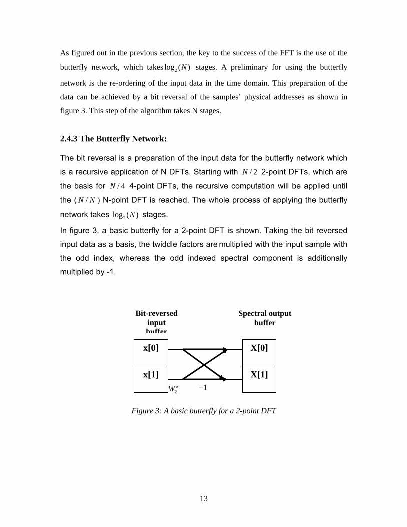
As figured out in the previous section, the key to the success of the FFT is the use of the
butterfly network, which takes 2log ( )N stages. A preliminary for using the butterfly
network is the re-ordering of the input data in the time domain. This preparation of the
data can be achieved by a bit reversal of the samples’ physical addresses as shown in
figure 3. This step of the algorithm takes N stages.
2.4.3 The Butterfly Network: The bit reversal is a preparation of the input data for the butterfly network which
is a recursive application of N DFTs. Starting with / 2N 2-point DFTs, which are
the basis for / 4N 4-point DFTs, the recursive computation will be applied until
the ( /N N ) N-point DFT is reached. The whole process of applying the butterfly
network takes 2log ( )N stages.
In figure 3, a basic butterfly for a 2-point DFT is shown. Taking the bit reversed
input data as a basis, the twiddle factors are multiplied with the input sample with
the odd index, whereas the odd indexed spectral component is additionally
multiplied by -1.
Figure 3: A basic butterfly for a 2-point DFT
x[0]
x[1]
X[0]
X[1]
2kW 1−
Bit-reversed input buffer
Spectral output buffer

14
Figure 4: Bit reversal of the input data
2.5 The Non-Uniform Discrete Fourier Transform (NDFT): The disadvantage of the DFT and FFT is the use of an evenly spaced frequency
range which leads into a transform of the whole frequency spectrum for the
sampling rate sf as a constraint. With the Non-Uniform Fourier Transform
(NDFT) it is possible, to analyze arbitrary frequency ranges with irregular
intervals. Therefore, an increase of accuracy is possible by the application of a
well-conditioned frequency vector.
000 x[0]
x[4]
x[2]
x[6]
x[7]
x[0]
x[1]
x[4]
x[5]
x[2]
x[3]
x[7]
x[6]
x[5]
x[3]
x[1]
000
001
010 010
011
001
011
100
100
111 111
101 101
110
110
Original input buffer
Bit-reversed input buffer
Bit-reversed address
of buffer elements
Original address of
buffer elements

15
Considering equation (11) of the DFT and taking the equidistant sampled
frequency domain in equation (9) into account with
k
s
f kf N
= 0,1,........, 1k N= − (14)
Where sf is the sampling frequency, N the number of samples and
0 1 1( ) [ , ,...., ]k Nf k f f f f −= = the arbitrary chosen frequency at k, the DFT can be
rewritten as a NDFT:
21 . .
0
[ ] [ ].k
s
N j f nf
n
X k x n eπ− −
=
= ∑ 0,1,........, 1k N= − (15)
The NDFT has still a complexity of 2N but due to the vector of arbitrarily chosen
frequencies, it is more accurate within the desired range. Everything outside that
range will be of a lesser accuracy but as this range is not required and can be
ignored. The vector itself holds the relevant frequencies of interest with well-
conditioned arbitrarily chosen frequencies in between these frequency points.
The interpretation of the NDFT’s results is raised by assigning the discrete non
equidistant spectral index value k directly to the arbitrarily chosen frequency
vector kf (16) after having estimated the spectrum.
0 1 1( ) [ , ,...., ]k Nf k f f f f −= = 0,1,........, 1k N= − (16)
2.6 The Goertzel Algorithm: Another effective derivative of the DFT is the Goertzel algorithm which found its
earliest formulation in 1958. It is a widely-used algorithm used for DTMF
applications. Different from DFT and FFT, the Goertzel algorithm does not regard
the whole frequency spectrum. These advantages can be used in the adaptation
of the Goertzel algorithm for musical systems, since the frequency range is also
known from 27.5Hz to 4186.01Hz as well as the number of expected frequencies

16
of interest which is 88. Therefore, it is only necessary to perform an analysis over
this range hence fewer points are required for the computation.
The Goertzel algorithm is a filter bench consisting of recursive second order
Infinite Impulse Response (IIR) filters. An example of these filters is depicted in
figure 6. Its system function can be deduced from its structure and is stated in
equation (17).
0 1
0 11 2
1 2
. .( )1 . .
b z b zH za z a z
− −
− −
+=
+ + (17)
Figure 5: Filter structure of the Goertzel algorithm
Table 2: Filter coefficients for the Goertzel algorithm
1z−
1z−
+
+
+
2a
0b
1b1a
[ ]kq n[ ]ky n[ ]x n

17
Inserting these coefficients into the system function and putting the value
of .k
s
fk Nf
= , the system function can be rewritten as:
. 1
1 2
1 .( , )1 2.cos( ).
kj w
k
e zH k zw z z
− −
− −
−=
− + 0,1,.....88k = (18)
The recursively calculated output signal finally is:
.[ ] . [ 1] [ 2] [ ] . [ 1]kj wk k k k ky k a q n q n x n e q n−= − − − + − − 0,1,.....88k = (19)
122.cos( . )a kNπ
=
2 1a =2. .
1
j kNb eπ
−= −
0 1b =
Feed forward section Recursive section

18
3. Implementation 3.1 The Digital Signal Processor (TI TMS320C6713 DSP): The Texas Instruments (TI) TMS320C6713 digital signal processor (DSP) is a 32
Bit floating point DSP of the C6000 series and runs at a frequency of 225MHz
and is optimized for audio applications. The DSP core contains two exclusively
fixed point Arithmetic-Logic Units (ALU), four both fixed and floating point ALU
and two both fixed and floating point multipliers. It can perform both in single and
double precision.
As in many commercially used processors, the TMS320C6713 has an 8KB
first level and a second level cache of 256KB as internal memory. The reason for
this unbalanced distribution of internal memory is that level 1 cache is on the
other hand fast and therefore contains both program and data cache, but is more
expensive compared to the level 2 cache on the other hand. Additionally, the
TMS320C6713 also has access to peripheral 16MB external Synchronous
Dynamic Random Access Memory (SDRAM) which can directly be accessed.

19
Figure 6: Memory Map for the TMS320C6713 DSP Starter KIT The user of the processor can choose between the two orders little and big
endian. That means, for the little endian mode (the default mode), the least
significant byte is stored at the lowest address, literally, little end first. In contrast
to this, in the big endian mode, the most significant byte is stored at the lowest
address, meaning, big end first.
The TMS320C6713 also makes use of an Enhanced Direct Memory Access
(EDMA) Controller. This technique enables the acquisition of audio data directly
from the stereo audio codec (AIC 23). The EDMA can also be combined with the
two Multichannel Bidirectional Serial Ports (McBSP)
Finally, the TMS320C6713 is provided with an optimized C/ C++ compiler for the
processor’s architecture. Especially the Multiply-Accumulate (MAC) command is
supported and the uses of this multiply and add combination (also known as sum
of products) is recommended.
3.2 The TI TMS320C6713 DSP Board
Internal Memory
Reserved Or
Peripheral
CPLD
SDRAM
Daughter card
0 90080000X
6713 DSK
Internal Memory
Reserved space Or
Peripheral Regs
EMIF CE0
EMIF CE1
EMIF CE2
EMIF CE3
C67X Family Memory Type
0 80000000X
0 90000000X
0 0000000XA
0 0000000XB
0 00030000X
0 00000000X
Address
Flash

20
The target hardware used for the analysis of frequency recognition algorithms is
the TMS320C6713 DSP Starter Kit, developed by Spectrum Digital and Texas
Instrument respectively, is referred as DSP board in the following. The reason
why not a Personal Computer (PC) (which nowadays has enough computational
power to compete with a DSP core), was not chosen for the analysis on
frequency recognition algorithms is because the aim was to target an embedded
solution. The Signal Processing Laboratory was provided with two of these DSP
boards by Texas Instruments. Due to financial restrictions, one further
requirement of the project was that the implementation of the frequency
recognition algorithms should be done on this board.
3.2.1 Chip Support Library (CSL): To handle interrupts, scheduling tasks and their priorities and to manage
memory, Texas Instruments has developed a DSP/BIOS real time operating
system. It operates independently from the application. All the settings for the
issues can be set up by a graphical configuration manager. When compiling, the
settings are then applied by the Chip Support Library (CSL).The software
interrupt (processBufferSwi) is defined or the software interrupt service routine
(ISR) which contains the frequency recognition algorithm.
3.2.2 The Code Composer Studio (CCS): The Code Composer Studio Code (CCS) is the front end of the TMS320C6713
DSP starter KIT and has a lot of advantageous properties.
The most obvious feature is the data visualization. The CCS offers the chance to
observe the data which are currently present in the internal buffers. In the
animation mode, even the change over time is recognizable,. i.e. a change in
frequency would change the diagrams, too.
Another, very important issue is the simple data import to and export capabilities
from these internal buffers. The latter scenario is very useful for debugging
purposes, i.e. for verifying results and frequency recognition algorithms either in
a simulation environment like MatLab or with an alternative ANSI C compiler.

21
This approach has been used in the course of the project and has been proved
to be the most effective way.
Furthermore, the CCS has the convenient feature of a simplified file I/O which
enables to trace results by using injections. Injections are soft breakpoint which
halt the CPU far a short moment to perform a file I/O. Like break and animation
points, they can just be used in a debug/release environment.
3.3 Usage of the Timer:
In order to use the 32-bit timer, two steps must be completed. At first, the timer
has to be configured and second a calibration has to be done which measures
the starting and the stopping of the timer itself.
There are three timer registers to be initialized: the control, the period and the
counter register. The timer control register is used to determine the timer’s mode.
The timer period register stores the maximum value the timer counts to. Once
this value is reached, a timer overflow occurs and the time measurements
become corrupt. The maximum value, a timer can maximal count is
0xFFFFFFFF. To circumvent a timer overflow, either the overflows have to be
counted or the number is downscaled through a division by constant, e.g. 1000.
This constant has to be bared in mind for the correction of the exported data. The
timer counter register stores the current value of the timer. To init the timer, the
constant 0x00000000 is to be taken.
The second step, the calibration of the timer in conjunction with the time
measurement is illustrated by

22
After having opened and having configured the timer as described above, the
timer needs to be calibrated because the measuring the time itself takes some
time, too. This calibration is the difference between two successive timer events,
i.e. the starting and the stopping of the timer. Then, the difference of both is
estimated, measured in cycles.
The actual measurement of the time works as follows. The timer is started, and
then the algorithm is performed. After having finished the calculation, the timer
stops again and the elapsed cycles are calculated out of difference of the start
time, the stop time and he calibration.
4. Implementation of the Frequency Recognition Algorithms 4.1 Methodology:
Open timer; Configure timer; Set timer to zero; Calibrate timer; Start timer; Stop timer; Calibration cycles = Stop – Start; Start timer; Perform algorithm; Stop timer; Elapsed cycles = Stop – Start – Calibration cycles; Close timer;
Figure 7: Pseudo code for applying time measurements

23
For the implementation of the algorithms, the real time characteristic is of less
importance in the first place. The main purpose is to get them working properly
and to verify their results in terms of correctness. In order to achieve this, several
tools are very useful.
As a first approach, MatLab and Simulink are consulted for a first implementation
of the algorithms. Their ease of use and their undisputable ability to monitor
results graphically very quickly are of assistance to get proof of the correctness
of the algorithms. The second step is a direct implementation of the algorithms in
ANSI C using Microsoft Visual Studio C++ 6.0. Since ANSI C is the programming
language which is used for developing applications for the Texas Instruments (TI)
TMS320C6713 Digital Signal Processor (DSP) core in the Code Composer
Studio (CCS), a fast implementation close to the final application is possible. This
step also ensures simultaneous debugging by taking a working algorithm as a
reference. This is a very effective way to verify intermediate steps. Since the
Code Compose Studio offers the opportunity to export complete buffer content’s
into text files, MatLab is used for verifying and displaying the results.
As input sources, several options can be considered. Cleary defined unique
sinusoids generated by WaveLab and played by the soundcard are valid input
signals. Signals from a signal generator are preferable though because they are
more reliable signal sources. At a later stage instrument samples playing musical
notes are taken as input source too
To summarize, for the implementation of the algorithms onto the target hardware,
MatLab and both developer studios (Microsoft Visual Studio C++ 6.0 and Code
Composer Studio go hand in hand) and complement each other. This methology
accelerates the developing process crucially and, what is also very important, it
helps to verify the results to make sure that they are correct.
4.2 Principle of the Frequency Recognition Algorithms

24
The process which all frequency recognition algorithms undergo can be
described as follows. At first, the sampled and quantized input signal ( )x n is
transformed into the frequency range, in order to obtain real { ( )}X nℜ and
imaginary part {X(n)}ℑ of its spectrum. The calculation of magnitude ( ( ))Mag X n is
initial for a peak detection mechanism, which finds the spectral component of the
signal with the maximum power. The index maxk of this spectral component is
finally evaluated with respect to the number of samples N and the sampling
rate sf . Since the frequency is now given as a numerical value, it is ideal for a
post processing MIDI conversion.
4.2.1 The Discrete Fourier Transform (DFT): 4.2.1.1 Simulation in Matlab: The Discrete Fourier Transform is defined as:
21 . . .
0
[ ] [ ].N j k n
N
n
X k x n eπ− −
=
= ∑ 0,1,.... 1k N= − (20)
and directly implemented in MatLab (appendix D). The result is shown in figure 8
depicting the original input signal, its spectrum together with the spectrum’s real
and imaginary part of a 1 kHz sinusoidal input at a sampling rate of 44100sf Hz= .
The signal is deliberately maximal non-coherent sampled as with a leakage
factor of 0.5 as explained in section, in order to obtain a maximum leakage effect.
It is noticeable that even under this worse case condition the peak detection
mechanism will succeed in terms of finding the maximum energetic spectral
component which underlines the decision not to apply extra windowing.

25
0 0.005 0.01 0.015
-0.5
0
0.5
t in s →
x(t)
in V
→
0 0.5 1 1.5 2
x 104
100
102
f in Hz →
|Mag
| in
dB →
0 0.5 1 1.5 2
x 104
-300
-200
-100
0
100
200
f in Hz →
Im{X
(f)} i
n dB
→
0 0.5 1 1.5 2
x 104
-400
-200
0
200
f in Hz →
Im{X
(f)} i
n dB
→
Figure 8: Frequency recognition in principle
4.2.1.2 Implementation of the DFT in C: A direct implementation of the DFT in C as in the case of the MatLab simulation
in the previous section is possible, however with slight differences. As MatLab
supports the scientific notation of complex numbers but since this convenient
implementation in C is not available, the twiddle factors have to be rewritten by
using the Euler equation:
2. . 2 2cos( . ) sin( . )
j kk NNW e k j k
N N
π π π−= = − (21)
This preliminary study is very important for the implementation of the DFT on the
TMS320C671 because the real and the imaginary part of the spectrum can be
regarded separately. Then the MAC (Multiply-ACumulate) command can be
applied as explained. Since the architecture and the compilers of the C6000
series are specialized for this product summing up command, an implementation

26
of the DFT in the way as described above is promising in terms of a fast
calculation speed.
What is more, as a consequence of the Nyquist-Shannon Theorem, only half the
calculated spectrum is relevant for an evaluation, more precisely, the frequencies
range of 0Hz until half the sampling rate / 2sf . Therefore, only a scan of half the
spectrum is necessary, a fact that results in an economization of computation
time.
4.2.2 The Fast Fourier Transform (FFT):
4.2.2.1 Simulation in MatLab: Since the Fast Fourier Transform (FFT) is a very efficient algorithm to apply the
Discrete Fourier Transform (DFT) by exploiting the redundancy of calculating the
twiddle factors, the approach to implement this algorithm implies previous
knowledge and understanding of the DFT.
For the simulation of the FFT, it reads wave files which contain signals to be
analyzed and outputs both its spectrum graphically and stores the input signal
numerically in a user defined output file. The intention is to take this numerical
data as a known reference for the implementation on the TI TMS320C6713.
Another derivative of this simulation has been used, but instead of referring to
wave files as input, actual buffer contents of the TI TMSC6713 were taken as the
input for the MatLab file. This method ensures a direct comparison of the
obtained spectra estimated both in MatLab and with the TI TMS320C6713 and is
very helpful for the development of the algorithm. 4.2.2.2 Implementation of the FFT in C: Since the implementation of the FFTW was not successfully applied, the
assembly coded library has to be taken for implementing the FFT. For this,
previous knowledge of the FFT as such is pre-requisite.

27
For a buffer size of N ≥ 32, where N has to be of the power of two, a N-point FFT
can be achieved. The API function DSPF_sp_cfftr2_dit() expects a pointer to an
input buffer, a pointer to an array holding the pre compiled twiddle factors and the
number of elements N as an integer as input parameters.
Since the input data has to be complex, i.e. consisting of interleaved real and
imaginary parts, the buffer containing this data has to have the length of 2 · N.
After the execution of this function, this buffer holds the complex result. The
number of twiddle factors is N/2 as a result of having taken advantage from their
redundant calculation. Per definition of the API, the twiddle factors have to be
reordered by bit reversal. Finally, after the calculation of the FFT, the output data
has to be reordered by bit reversal. Both twiddle factor pre calculation and bit
reversal can be found in the TI FFT support files.
Since there was no need to implement the FFT explicitly in another development
environment rather than the Code Composer Studio (CCS), the DFT has been
taken as a reference for the development of the FFT. The approach is, to export
the input buffer of the algorithm in the CSS and to re-import them into the
alternative development environment. Then, a debugging close to real conditions
is possible.
4.2.3 The Non-Uniform Discrete Fourier Transform (NDFT): The structure of the Non-Uniform Discrete Fourier is similar to the DFT and its
complexity is 2N , as well. The only difference is the fact that the NDFT does not
refer to an equidistant sampled frequency range indexed with k but to an
arbitrarily frequency vector kf as described. It is expected that the assessing to
this vector stored in an array causes an additional delay that makes the NDFT a
bit slower than the DFT.
The main issue of the NDFT and the key for its advantage in comparison to the
DFT is the arbitrarily chosen frequency vector whose accuracy is increased, if it
is ellconditioned. For frequencies in the lower range (i.e. 27.5Hz, 29.14Hz, … ), a
finer fragmentation of the frequency vector is required, because the spacing

28
between two neighboured notes is smaller than for adjoining frequencies in the
higher range (i.e. … 3951.07Hz, 4186.01Hz).
The main problem is the fact that there are 88 MIDI notes, a number which differs
from the buffer size N in every case. If the buffer size N was equal to 88, each
MIDI note would correspond to a buffer index, but this is, as mentioned before,
not possible. For a buffer size N less than 88, the accuracy would not be
sufficient enough due to the fact that some of the MIDI notes are simply not
assigned to one buffer index. The most interesting case is, if the buffer size is
greater than the number of MIDI notes.
The spacings between each frequency point between two MIDI notes are
equidistant though, however dissimilar between each MIDI note pair due to the
fact that the MIDI notes themselves are not equidistant arranged to each other.
Taking equation (1) with as a69
12( ) 440.2M ID In
M ID If n H z−
= basis, the spacings
are calculated in dependence on two neighbored MIDI notes and the buffer size
N.
( 1) ( )( )
88MIDI
MIDI MIDIn
f n f nN N+ −
Δ = 21 108MIDIfor n≤ ≤ (22)
Figure 9: Arbitrarily chosen frequencies for the NDFT

29
The final structure of the vector holding the arbitrarily chosen frequencies and the
corresponding MIDI notes is shown in figure 9 in principle. Since this vector is
dependent on the buffer size N, it has to be recalculated for each buffer size N.
4.2.4 The Goertzel Algorithm: Before coding the Goertzel algorithm up, it is quite useful to have a closer look at
the Goertzel IIR filter coefficients as they are listed in table 3 . Since the filter
coefficients b0 = 1 and a2 = -1 remain constant throughout the whole calculation
and hence do not have to be determined at each stage, the filter coefficients b1
and a1 have to be calculated only for each Goertzel filter. It is useful to separate
the complex denotation of filter coefficient b1 into a real and an imaginary part
using the Euler equation as shown in equations (41) and (42).
2 .2 .. .
1
k
s
fjj k fNb e eπ π−−
= − = − 0,1,.....88k = (23)
1 1 1cos(2 . ) .sin(2 . ) ( ) . ( )k k
s s
f fb j b j bf f
π π= − + = ℜ + ℑ 0,1,.....88k = (24)
For the sake of completeness, filter coefficient a1 of the recursive section is given as
122cos( . )a kNπ
= (25)
This consideration results in a set of 3 · 88 = 264 pre-calculated filter coefficients
to be set up in a look-up table as shown in principle in table 3.
Table 3: Frequencies and filter coefficients for 88 MIDI notes

30
For the buffer size N, the signal is filtered with respect to the pre-calculated filter
coefficients. Since only the real and imaginary part and their magnitude are of
interest only, a calculation of these intermediate values takes place after having
filtered the data. Different from DTMF systems using 8 frequencies of interest,
the maximum number of the frequencies to be regarded is 88. For reason of
saving computation time, the pre- calculated filter coefficients are read from a two
dimensional array goertzel_coeff for each loop pass. It has been shown that the
speedup of the method of pre calculation the IIR filter coefficients results in a
considerable factor of 210 .
The actual Goertzel value is obtained with the application of the Goertzel IIR filter
by taking the filter coefficients into account. Again, as considered in section 3.4,
the estimation of the maximum power happens promptly without and is
continuously updated if the maximum is excelled instead of a down streaming
scanning of a whole temporary buffer containing all successively calculated
Goertzel values.
4.3 Comparison of schedulable Buffer Sizes: A noteworthy fact is the actual memory requirement for a buffer size N for each
of the algorithms. This also demonstrates the reason why a maximum buffer size
of just 8192 can be applied.
To obtain N data elements, the ping and the pong buffer have to be set up,
each of a size of 2.N . Due to the codec only applying a stereo input, twice the
number of samples as to be scheduled. In total, for the DFT and the Goertzel
algorithm, the actual buffer equirements are 4 · N.
31
In particular in the case of the FFT, for the generation of the input buffer for
the API function, another additional buffer is needed. This buffer has the size
of 2.N , because the input data has to be complex with interleaved real and
imaginary part. The twiddle factors need an extra buffer of the size / 2N . In total,
5.5 times more data elements have to be provided than originally scheduled for a
problem size N.
The NDFT has, due to its complexity, similar basic memory requirements of
(4. )N as the DFT. Additionally, there is a need of N data elements for the pre-
calculated arbitrarily chosen frequency vector.
Table 11 lists the actual buffer size requirements for a problem size N and
states which factor has to be taken into consideration for an implementation of a
problem size N for each algorithm.
5. Measurements In order to obtain distinct signals consisting of single sinusoids only, a common
signal generator is used. For monitoring reasons its signals are simultaneously
displayed with an oscilloscope. Once the signal has been led into the line input of
the Texas Instruments (TI) TMS320C6713 Digital Signal Processor (DSP) board
it is subject to sampling and quantization before it can be analyzed by one of the
to be investigated by one of the to be investigated frequency recognition
algorithms. The development software, naming the Texas Instruments’ Code
Composer Studio is installed on the PC and is used for both coding the
algorithms and for storing the measurement results in a file. 5.1 Analysis of Input Signals: Measurements without any preceding estimation or even without a basic analysis
are useless. In other words, starting a measurement without any kind of
expectancy is neither engineer-like nor scientific. Therefore, this section analyses
the input signals’ spectra versus time, i.e. the spectral behavior during the
duration of the samples. It does not take into account the spectral resolution. It

32
makes assumptions of the algorithms’ frequency recognition capability
exclusively based on an analysis of the input signals’ spectra and is therefore a
hypothesis. By doing this, a necessary preliminary evaluation of the frequency
recognition algorithms is possible.
It is presumed that the first category of signals, which consists of a simple
sinusoid, are stable over their whole duration, meaning, a simple maximum
power search over the spectrum will yield the fundamental frequency. That is
why, for this type of signal, frequency recognition is expected to be without
complications.
For the second category, signals containing complex waveforms, samples of
notes played by musical instruments are used as an input for the frequency
recognition algorithms. The expectation is that not every sample holds the
maximum power on the fundamental frequency because the signal can no longer
be considered to be a simple sinusoid. Moreover, for some of the notes some of
the harmonics actually carry more power. Additionally, this behaviour changes
over time for some of the regarded notes, which might make frequency
recognition more difficult rather than with simple sinusoids. These assumptions
have to be confirmed both by the following spectral examination and verified by
the measurements itself.
5.1.1 Sinusoidal Inputs: The bases for the evaluation of the frequency recognition algorithms are the
metrics latency, speedup and accuracy as discussed earlier. Latency and
speedup can be deduced from the number of cycles an algorithm needs to
estimate a frequency and the accuracy depends directly on the algorithmic
estimation capability from which the absolute deviation can be calculated.
To find out the best frequency recognition algorithm, at least 10 test series for
each buffer size for 32 ≤ N ≤ 8192 have been applied to each algorithm. The
reasons for these boundaries are as follows. The lower bound 32 ≤ N is a
limitation of the implementation of the FFT API routine (DSDF_sp_cfftr2_dit) from
Texas Instruments (TI), whereas the upper bound is due to internal memory
33
constraints. Furthermore, for a buffer size of N > 8192, there would be
unreasonably high computational costs for the calculation of direct frequency
recognition algorithms such as the DFT and the NDFT, whose costs are N2.
Concluding, the common boundaries for the buffer size, 32 ≤ N ≤ 8192, have
been chosen for all the measurements to be able to compare all the algorithms
and should be sufficient to fulfill the task.
For each algorithm test series, three cases were investigated: the note A4 with
440Hz (being the note in the centre of the MIDI scale), and two extreme cases:
the highest frequency with 4186.01Hz (note C8) and the lowest one of 27.5Hz
(note A0) of the target frequency range. The reason for these choices is to
determine the ability to analyze the algorithms’ capability to handle the highest
frequency, 4186.01Hz and the highest spectral resolution demand at 27.5Hz,
However, there are a number of harmonics along with the fundamental frequency
which should not occur. When we are considering the input from the function
generator. The reason for this is the fact that the signal generator does not
produce a pure sinusoid exclusively but has a small amount of harmonic
distortion and should be ignored in this case. Additionally, there are reflections
due to a mismatched connection from the signal generator to the audio jackinput
of the DSP board. But here we are not considering the function generator but
taking the signal directly from the system. Since the maximum power can be
found at 440Hz, 4186.01Hz and 27.5Hz respectively, these undesired, less
powerful frequencies do not carry weight in terms of frequency recognition. This
is a good prerequisite for a solid frequency recognition capability regardless of
the spectral resolution in terms of accuracy and a reasonable buffer size N.
5.1.2 Inputs of Musical Instruments: For signals containing simple sinusoids generated by a signal generator, it is
anticipated that the frequency recognition algorithms should work perfectly if
maximum power detection is used. Whether they can be applied to signals
containing complex waveforms is subject to a discussion in this section.

34
To test the frequency detection capabilities of each algorithm, four different
instruments (piano, violin, trumpet and flute) playing three different notes have
been taken as an input. Because not every note of the frequency range of
interest can be subject to an analysis and a subsequent measurement, because
of the range of each instrument, a representative selection has to be made.
Thus, all the selected notes are played by each instrument to ascertain
comparability.
When applying instrumental inputs, the frequency recognition capability is initially
of interest only. The buffer size N is dependent on the demand for the accuracy
for the notes C6, C5 and C4 respectively. Equation (44) denotes the coherence
between the sampling rate sf and the demanded accuracy depending on the
MIDI note.
( )s
MIDI
fNaccuracy n
= (26)
Table 13 lists summarizing the constraints of the notes which are subject to
further measurements. They are valid each for piano, violin, trumpet and flute.
Table 4: Frequencies and filter coefficients for 88 MIDI notes
35
5.2 Prediction of the Algorithms’ Frequency Recognition Capability: Taking simple sinusoids (440Hz, 4186.01Hz and 27.5Hz) all frequency
recognition algorithms have an unambiguous input because the spectral
distribution of the signal’s power remains constant throughout the whole time
window and spectrum’s maximum peak can be found at the fundamental
frequency. That is the reason why the chances of failure are very low using only
a simple power detection technique. Measurements on the algorithms with these
sinusoidal inputs and the subsequent analysis with the evaluation criteria will give
certainty whether this prediction is right.
For instruments playing musical notes, it is important to find out whether the
maximum power can actually be found on the fundamental frequency or on one
of its harmonics. In the latter case, investigations have shown that the lower the
frequency is the more harmonics exist. For all analyzed musical notes
(1046.5Hz, 523.23Hz and 261.63Hz), string-based instruments (piano and violin),
the spectral behavior over time is constant and therefore ideal for frequency
recognition. It can also be seen, that the relative power distribution of the
spectrum of these string based instruments remains stable over time, i.e. the
maximum power can always be found on the fundamental frequency of the note
being played. However, the spectrum over time of woodwind and brass
instruments like the flute and the trumpet respectively is not well behaved for
each of the analyzed notes. The trumpet does not have the maximum power on
the fundamental frequency for MIDI note C5. Furthermore, for MIDI note C4, both
the trumpet and the flute will fail according to the preliminary spectral analysis
because the maximum power is not held by the fundamental frequency each.
Table 5 lists the probable frequency recognition capabilities of the investigated
algorithms with respect to the analyzed instrumental notes.
Table 5: Probable frequency recognition capability of instruments

36
5.3 Evaluation Criteria In order to find the optimum frequency recognition algorithm, there is a need for a
precedent definition of fixed quantities and performance metrics. The purpose is
a reduction of the number of variables to a reasonable minimum which is then
subject to a further analysis. Finally, this preliminary investigation leads to the
conclusion that the evaluation criteria, in particular the performance metrics, are
dependent on the buffer size N only.
5.3.1 Sampling Rate: The sampling rate is fixed to 44100sf Hz= in order to take into account high
frequency harmonics, since the analysis of frequency recognition algorithms is
subject to a further extension to the whole audible range of 0Hz – 22000Hz.
Therefore the sampling rate has to be greater than twice the maximum frequency
that can appear in the expected signal in order to avoid aliasing according to the
Nyquist-Shannon theorem as explained in section 5.4.1.1. Consequently, this
major constraint of having a sampling rate of 44100sf Hz= is mandatory for the
Generic Musical Instrument System (GMIS), despite of having a large buffer size
N and thus having an increase of complexity, because the higher the sampling
rate, the more sampling points are acquired.
5.3.2 Spectral Resolution:

37
A fine spectral resolution R is prerequisite for a solid accuracy and is given by the
ratio of the sampling rate sf and the actual buffer size N with
( , ) ss
fR f NN
= (27)
In general, one can say, the higher the buffer size N the better is the spectral
resolution R at a given sampling rate sf . Due to the fact that an increase of the
buffer size N simultaneously causes an increase of computational costs and
memory requirements, a trade-off has to be found between the spectral
resolution, R, and the buffer size, N.
When analyzing musical notes, the maximum spectral resolution which has to be
provided, is max 0.82R Hz= in order to be able to recognize all frequencies of the
whole target frequency range. The reason for this high resolution is the smallest
half of the MIDI channels, i.e. between MIDI note #21 and #22 with 27.5Hz and
29.14Hz respectively.
5.3.4 Time to settle: The system’s time to settle settlet is the time which is needed to make sure that the
buffer completely holds the signal’s samples. This quantity is relevant and
subject to further investigations for unbuffered systems only, but because internal
buffers are applied, settlet is constant the time required for filling up a buffer of the
size N. Let the sampling frequency be 44100sf Hz= and assuming there is a
buffer of the size N = 44100, it takes one second to acquire all 441000 samples.
Therefore, the time to settle settlet is defined as
settles
Ntf
= (28)
As the sampling rate sf is fixed to 44100Hz and the buffer size N does not
change during the operating mode, the time to settle settlet is constant for each
buffer size N, too.

38
5.3.5 Computational Costs of Investigated Algorithms: The complexities of the to be investigated algorithms are listed for the buffer size N
Table 6: Fourier transform-based algorithmic complexity
The comparison of the complexities of the Goertzel algorithm and the FFT
shows, that at a buffer size of N > 288, the FFT’s algorithmic complexity will be
greater than the one of the Goertzel algorithm, but the buffer size required for this
problem is unreasonable high and furthermore not feasible without massive
accessing external memory. This, however, would mean additional latencies and
would be a different kind of problem which cannot be taken into consideration at
this stage.
Theoretically, the number of cycles corresponds directly to the algorithmic
complexity, but there is an additional amount of cycles for pre and post
processing of audio data to be regarded, for instance the generation of
interleaved complex data, the calculation of magnitude, the spectrum’s peak
detection and the final evaluation of the most powerful spectral frequency
component given as an index. Thus, the overall number of cycles has to be
measured and taken into account when analyzing the metrics.
Discrete Fourier Transform (DFT)
Fast Fourier Transform (DFT)
Non-Uniform Discrete Fourier Transform (DFT)
Goertzel algorithm
Algorithm Complexity
88.N
2log ( )N N
2N
2N

39
5.4 Performance Metrics For the evaluation of a system’s real time characteristics, it is necessary to take
the algorithmic properties into account, i.e. their latency, their speedup and the
algorithms’ accuracy. These metrics are subject to be discussed in this section.
It is expected that according to the fixed computational costs of each
algorithm the number of cycles needed for the calculation of each algorithm, will
follow the same law. Consequently, the tendencies of speedup and latency will
remain equal with each measurement and independent from the input, but due to
the fact that the number of cycles are deduced from the computational cost and
are therefore theoretical, they have to be experimentally proven. Therefore and
with respect to the fact that pre and post processing of the data is not included to
the theoretical considerations, there is an extra need for measuring these
metrics.
5.4.1 Latency: The latency is the time a signal needs to get from its source to its destination
after processing. In the case of frequency recognition as applied in this project,
latency is the difference in time between playing the note and detecting its
frequency or in other words how long an algorithm needs to output the numerical
value of the estimated frequency. Therefore, for the number of cycles an
algorithm takes, the latency is defined as
CPU
cyclesltf
= (29)
with a given central processing unit (CPU) frequency of the TI TMS320C6713 of
225CPUf MHz= . The average in latency averagelt is the average temporal resolution
of a human ear, i.e. the time that can pass by before the listener realizes a delay
in playing a note and hearing the actual sound. It has been shown that on
average the latency of the human ear is 50averagelt ms= . Consequently, in order to
be taken seriously into consideration for frequency recognition in real time, the

40
algorithms have to terminate their calculations within this time limit, preferably
less than that because frequency recognition will probably not be the only task
for the GMIS. 5.4.2 Speedup: An important metric for the evaluation of is the speedup according to Amdahl’s
Law. The speedup is the ratio of the number of cycles of an algorithm before and
after its improvement and is described as
DFTcyclesspcycles
= (30)
The speedup has to be greater than 1 if the algorithm is to be considered
superior to any of the other investigated algorithms. Due to the fact that the
Discrete Fourier Transform (DFT) is the slowest Fourier transform-based
algorithm, it is taken as a baseline for the speedup for all the other algorithms.
5.4.3 Accuracy: A measure for the accuracy is the absolute deviation. The absolute deviation of a
value in a set of values is the absolute difference between this value and a
nominal. This nominal can either be a mean of the set of these values or a
threshold value, in this case the expected frequency epf . The value from which
the absolute difference is taken is the estimated frequency esf . Being a measure
for accuracy, absolute deviation is defined as
ep esad f f= − (31)
Due to the fact that the tolerance is the half the difference between two MIDI
channels, in the worse case between MIDI note #21 and #22, the minimum
acceptable error equals the maximum spectral resolution required for accurate
frequency recognition, min max. . .82i e ad R Hz= = .

41
6. Results The first category, input signals consisting of a simple sinusoid, is used to
measure latency and speedup in the first step in order to prove the theoretical
complexity discussed earlier and second to show the functionality of the
investigated frequency recognition algorithms, i.e. to prove their frequency
recognition capability and to investigate on their accuracy as derived earlier.
The second category, instrumental inputs playing musical notes, is taken to judge
on the algorithms’ frequency recognition capability for input signals containing
complex waveforms such as in the case of musical notes. By doing this, it will be
demonstrated that a simple frequency recognition algorithm with simple peak
power detection as performed in the first set of measurements, will not suffice for
a musical system as proposed with the GMIS.
6.1 Frequency Recognition Algorithms analyzing simple Sinusoids
6.1.1 Latency: The behavior of the algorithmic latency depends on their individual complexity as
described earlier. For the regarded frequencies 27.5Hz, 440Hz and 4189Hz, the
latency is equal as it can be seen in figures 10 - 12 which underlines the
preliminary considerations earlier. Therefore, just an analysis of the results
concerning the latency’s tendencies for each algorithm is made, not for each
frequency in particular.
Figures 10 - 12 show the four algorithms’ latency versus the buffer size N for
different inputs containing simple sinusoids of 440Hz, 4186.01Hz and 27.5Hz
respectively. The algorithms with the maximum latency for the whole range of N,
with 32 ≤ N ≤ 8192, are the DFT and the NDFT with a narrow difference to the
advantage of the DFT as expected. This slight difference is due to the fact that

42
the NDFT has to read the vector with the arbitrarily chosen frequencies whereas
the DFT simply uses the equidistant spectral index k for the computation of the
spectrum. According to their equal structure, the tendency of their latencies is
equal, too. The Goertzel algorithm has a smaller latency than the DFT and NDFT
but is, as expected, still slower than the FFT.
Figure 10: Latency vs. Buffer size for a 27.5Hz input
0 1000 2000 3000 4000 5000 6000 7000 8000 900010-5
10-4
10-3
10-2
10-1
100
101
102
buffersize(N)
late
ncy
latency vs buffersize for inoput of 27.5HZ

43
Figure 11: Latency vs. Buffer size for a 440Hz input
Figure 12: Latency vs. Buffer size for a 440Hz input
0 1000 2000 3000 4000 5000 6000 7000 8000 900010-5
10-4
10-3
10-2
10-1
100
101
102
buffersize(N)
late
ncy
latency vs buffersize for inoput of 4186.01hZ
0 1000 2000 3000 4000 5000 6000 7000 8000 900010-5
10-4
10-3
10-2
10-1
100
101
102
buffersize(N)
late
ncy
latency vs buffersize for inoput of 440
***FFTDFT
ND FT
* Goertzel

44
6.1.2 Speedup: Figures 13- 15 show the speedup with respect to the buffer size N for 440Hz,
4186.01Hz and 27.5Hz. Again as expected, since the speedup is also directly
linked with the number of cycles, the three graphs are fairly equal for each input
frequency.
Taking the DFT as a baseline, just the NDFT is slightly slower which is due to
implemental reasons, i.e. the reading of the vector of the arbitrary chosen
frequencies takes more time than just simply referring to a loop index.
The Goertzel algorithm with a complexity of 88·N is dramatically faster than the
DFT and the NDFT which computational costs are 2N , but is still more slowly
than the FFT with a complexity of 2log ( )N N , again as expected.
Figure 13: Speedup vs. Buffer size for a 27.5Hz input
0 1000 2000 3000 4000 5000 6000 7000 8000 900010-1
100
101
102
103
104
buffersize(N)
spee
d
speed vs buffersize for 27.5Hz

45
Figure 14: Speedup vs. Buffer size for a 440Hz input
Figure 15: Speedup vs. Buffer size for a 4186.01Hz input
0 1000 2000 3000 4000 5000 6000 7000 8000 900010-1
100
101
102
103
104
buffersize(N)
spee
d
speed vs buffersize for 4186.01Hz
0 1000 2000 3000 4000 5000 6000 7000 8000 900010
-1
100
101
102
103
104
buffersize(N)
spee
d
speed vs buffersize for 440Hz
***FFTDFT
ND FT
* Goertzel

46
6.1.3 Accuracy: Why can the fastest algorithm, the FFT, not simply be taken for frequency
recognition? The answer is that, the less time an algorithm needs to fulfill its
purpose the better it is, but it still has to be accurate enough to meet the
requirements. Thus, the accuracy of each algorithm’s frequency recognition
capability has to be analyzed, too, because a fast but inaccurate algorithm is of
no use. As defined, a measure for accuracy is the absolute deviation of the
estimated frequency from the expected frequency, i.e. the absolute difference
between these both frequencies.
0 1000 2000 3000 4000 5000 6000 7000 8000 9000101
102
103
estim
ated
freq
uenc
y(H
z)
buffersize(N)
estimated frequency vs buffersize for input of 27.5Hz

47
Figure 16: Estimated frequency vs. Buffer size for a 27.5Hz input
Figure 17: Absolute deviation vs. Buffer size for a 27.5Hz input
0 1000 2000 3000 4000 5000 6000 7000 8000 9000
102.2
102.3
102.4
102.5
102.6
102.7
102.8
102.9
buffersize(N)
estim
ated
freq
uenc
y(H
z)
estimated frquency vs buffersize for input of 440Hz
0 1000 2000 3000 4000 5000 6000 7000 8000 900010-1
100
101
102
103
buffersize(N)
abso
lute
dev
iatio
n(H
z)absolute deviation vs buffer size for input of 27.5Hz
***FFTDFT
ND FT
* Goertzel

48
Figure 18: Estimated frequency vs. Buffer size for a 440Hz input
Figure 19: Absolute deviation vs. Buffer size for a 440Hz input
Figure 20: Estimated frequency vs. Buffer size for a 4186.01Hz input
0 1000 2000 3000 4000 5000 6000 7000 8000 9000103.54
103.56
103.58
103.6
103.62
buffersize(N)
estim
ated
freq
uenc
y(H
z)
estimated frequency vs buffer size for input of 4186.01Hz
0 1000 2000 3000 4000 5000 6000 7000 8000 9000100
101
102
103
abso
lute
dev
iatio
n(H
z)
buffersize(N)
absolute deviation vs buffersize for input 440Hz
***FFTDFT
ND FT
* Goertzel

49
Figure 21: Absolute deviation vs. Buffer size for a 4186.01Hz input 6.1.4 Comparison of the Investigated Metrics: From the results presented, it can be seen that the DFT and the NDFT yield the
highest latency due to their equal structure. The NDFT is slightly slower, the
speedup with respect to the DFT is 0.933 on average which is due to the
additional reading of the vector with the arbitrarily chosen frequencies. The
Goertzel algorithm is considerably faster than the DFT and NDFT but definitively
slower than the FFT. Its tendency of latency and speedup is due to its algorithmic
complexity of 88·N. The fastest frequency recognition algorithm is clearly the FFT
with a complexity of 2log ( )N N .
The DFT is far too slow and inaccurate and is therefore as expected not to be
taken into account for frequency recognition at all. The NDFT has an adequate
accuracy at a buffer size of N = 4096, but is too slow for the average latency of
the human ear. The most interesting case is the frequency input of 27.5Hz,
where an accuracy of 0.82Hz is demanded. It has been clearly shown that the
0 1000 2000 3000 4000 5000 6000 7000 8000 9000100
101
102
103
buffersize(N)
absl
oute
dev
iatio
n(H
z)absolute deviation vs buffersize for 4186.01Hz
***FFTDFT
ND FT
* Goertzel

50
FFT, the DFT and the Goertzel algorithm fail in terms of accuracy. For these two
algorithms, a buffer size of N > 8192 is necessary to meet the constraints. The
NDFT, however, is accurate enough for the demanded spectral resolution of
0.82Hz but is far too slow and beyond the maximum allowed latency of 50ms.
6.2 Frequency Recognition Algorithms analyzing Musical Notes The question is whether the frequency recognition algorithms are able to cope
with instrumental inputs. As analyzed, it has been analytically shown that the
spectrum for a single note over time can join the maximum power on one of their
harmonics rather than on the fundamental frequency, depending on the
instrument’s character.
6.2.1 Note C6 (1046.5Hz) for Piano, Violin, Flute and Trumpet: Figure 22 - 23 depict the estimated frequencies over time for an 1046.5Hz input
played by the two string based instruments piano and violin respectively. Since
the estimated frequency is within the boundaries throughout the whole sample’s
duration, all investigated frequency recognition algorithms meet the restrictions
for all applied instrumental inputs.
0 0.1 0.2 0.3 0.4 0.5 0.6 0.7 0.8 0.9 1
103.015
103.017
103.019
103.021
103.023
103.025
103.027
Estimated frequency(Hz) vs time for input of 1046.25Hz(panio)
Est
imat
ed fr
eque
ncy(
Hz)
t(s)

51
Figure 22: Estimated frequency vs. time for a 1046.5Hz input (piano)
Figure 23: Estimated frequency vs. time for a 1046.5Hz input (violin) The Goertzel algorithm is the most accurate algorithm and estimates 1046.5Hz
constantly during the whole sample’s duration. The FFT is the frequency
recognition algorithm with the nearest close accuracy with an estimated
frequency of 1033.99Hz for every moment. The DFT and the NDFT meet the
constraints in terms of accuracy, too.
0 0.5 1 1.5 2 2.5 3 3.5103.01
103.02
t(s)
Est
imat
ed fr
eque
ncy(
Hz)
Estimated frequency(Hz) vs time for input of1046.5Hz(violin)
*** FFTDFT
NDFT

52
Figure 24: Estimated frequency vs. time for a 1046.5Hz input (trumpet)
Figure 25: Estimated frequency vs. time for a 1046.5Hz input (flute)
*** FFTDFT
NDFT
0 1 2 3 4 5 6 7
103.02
103.03
103.04
Estimated frequency(Hz) vs time for input of 1046.5Hz(trumpet)
Est
imat
ed fr
eque
ncy(
Hz)
t(s)
0 0.5 1 1.5 2 2.5 3 3.5103.01
103.02
t(s)
estim
ated
freq
uenc
y(H
z)
estimated frequency vs time for input of 1046.5Hz(flute)

53
Both the DFT and the NDFT show a similar behaviour like for the string. Both
algorithms are accurate enough for meeting the restrictions but they are
fluctuating throughout the whole sample’s duration, whereas the DFT appears
more stable than the NDFT. Again, the FFT supplies accurate frequency
estimation within the limits, but is subject to variation for a violin. The only
algorithm, which is unreliable in terms of frequency recognition for woodwind and
brass instruments, is the Goertzel algorithm.
6.2.2 Note C5 (523.25Hz) for Piano, Violin, Flute and Trumpet: For a string based instrumental input of 523.25Hz all algorithms succeed in
estimating the played note, as shown is figures 26 and 27. Again, the Goertzel
algorithm is the most accurate and hits exactly the expected frequency of
523.25Hz. The FFT is similar to the previous section the next close frequency
recognition algorithm and estimates constantly 517.0Hz over the whole samples’
duration and hence meets the given constraints. As expected, the DFT and the
NDFT fluctuate but are is still in between the upper and lower bounds of
508.57Hz and 537.93Hz respectively.
0 0.2 0.4 0.6 0.8 1 1.2 1.4 1.6 1.8
102.714
102.716
102.718
102.72
102.722
102.724
102.726
Estimated frequency(Hz) vs time for input of 523.25Hz(piano)
Est
imat
ed fr
eque
ncy(
Hz)

54
Figure 26: Estimated frequency vs. time for a 523.25Hz input (piano)
Figure 27: Estimated frequency vs. time for a 523.25Hz input (violin) Regarding the measurement results for the flute and the trumpet, a more specific
evaluation is required. Figure 28 shows the estimation capabilities of the four
algorithms for a flute playing MIDI note C5. The DFT, the FFT and the NDFT are
vacillating but are within the desired absolute tolerance of 14.68Hz, meaning that
the estimated frequency does not cross the upper and lower limits of 508.57Hz
and 537.93Hz respectively at any time. In specific, the FFT is the least fluctuating
algorithm. In contrast to these three algorithms, the Goertzel algorithm fails in
terms of accuracy.
For all algorithms, the estimated frequency wobbles between these two
harmonics. Consequently, for a trumpet playing MIDI note C5 it is impossible to
estimate the expected frequency of 523.25Hz regardless what algorithm is being
applied.
0 0.5 1 1.5 2 2.5 3
102.711
102.714
102.717
102.72
102.723
102.726
Estimated frequency(Hz) vs time for input of 523.25Hz(violin)
Est
imat
ed fr
eque
ncy(
Hz)
*** FFTDFT
NDFT

55
Figure 28: Estimated frequency vs. time for a 523.25Hz input (flute)
0 0.5 1 1.5 2 2.5 3 3.5
102.7
102.71
102.72
102.73
102.74
Estimated frequency(Hz) vs time for input of 523.25Hz(flute)E
stim
ated
freq
uenc
y(H
z)
t(s)

56
Figure 29: Estimated frequency vs. time for a 523.25Hz input (trumpet) 6.2.3 Note C4 (261.63Hz) for Piano, Violin, Flute and Trumpet: For a string based input of a piano and a violin playing note C4 (261.63Hz) the
DFT, the FFT and the NDFT meet the limits given by the absolute tolerance of
7.34Hz. The DFT varies within the compulsory boundaries of 254.29Hz and
268.97Hz respectively, and so does the NDFT but more modest than the DFT.
The FFT is not fluctuating at all and stays constant at an estimated frequency of
258.5Hz. However, the Goertzel algorithm does not fulfill the required constraints
at each moment and is therefore not reliable for recognizing the input’s frequency
for these two instruments.
2 3 4 5 6 7 8 9
103.02
103.05
103.08
103.11
103.14
103.17
Estimated frequency(Hz) vs time for input of 523.25Hz(trumpet)E
stim
ated
freq
uenc
y(H
z)
*** FFTDFT
NDFT
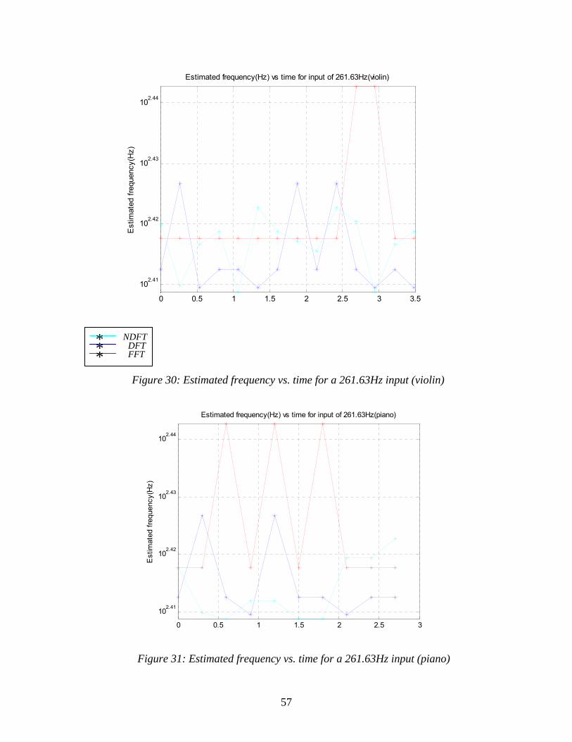
57
Figure 30: Estimated frequency vs. time for a 261.63Hz input (violin)
Figure 31: Estimated frequency vs. time for a 261.63Hz input (piano)
0 0.5 1 1.5 2 2.5 3 3.5
102.41
102.42
102.43
102.44
Estimated frequency(Hz) vs time for input of 261.63Hz(violin)
Est
imat
ed fr
eque
ncy(
Hz)
0 0.5 1 1.5 2 2.5 3
102.41
102.42
102.43
102.44
Estimated frequency(Hz) vs time for input of 261.63Hz(piano)
Est
imat
ed fr
eque
ncy(
Hz)
*** FFTDFT
NDFT

58
All the algorithms estimate these both overtones at 1046.5Hz and 1569.98Hz
respectively because of the reasons stated above. Hence and to anticipate at this
stage, a simple application of the frequency recognition algorithms is not
sufficient when playing note C6 with a trumpet.
Figure 32: Estimated frequency vs. time for a 261.63Hz input (flute)
0 0.5 1 1.5 2 2.5 3 3.5
102.714
102.716
102.718
102.72
102.722
Estimated frequency(Hz) vs time for input of 261.63Hz(flute)E
stim
ated
freq
uenc
y(H
z)

59
Figure 33: Estimated frequency vs. time for a 261.63Hz input (trumpet)
6.2.4 Comparison of Frequency Recognition Capability for Musical Notes: The DFT, the FFT and the NDFT are able to estimate the expected frequency
within the given constraints for note C6 for each instrument; for note C5 for all
instruments except the trumpet and for C4 for string based instruments only, i.e.
the piano and the violin.
Also, as expected, all algorithms fail in terms of estimating the fundamental
frequency for the trumpet playing note C5 and even for both flute and trumpet
producing note C4 due to the fact that the maximum power for the notes played
by these instruments is joined at their harmonics as shown. In particular, note C5
(523.25Hz) played by a trumpet, holds its maximum power on its second
harmonic 1046.5Hz as analytical shown and experimental verified. In specific, for
note C4 (261.63Hz) played by a flute, the maximum power can be found at the
second harmonic at 523.25Hz, the reason why the peak detection mechanism of
all algorithms estimates this frequency. For a trumpet playing note C4, it has
been theoretically and experimentally shown that it is even more difficult to find
0 1 2 3 4 5 6 7 8103.02
103.05
103.08
103.11
103.14
103.17
Estimated frequency(Hz) vs time for input of 261.63Hz(trumpet)
Est
imat
ed fr
eque
ncy(
Hz)
*** FFTDFT
NDFT
60
the correct expected frequency because the maximum power is present at both
the fourth and sixth harmonic of 1046.5Hz and 1569.98Hz respectively.
The exception is the Goertzel algorithm. It identifies the correct frequency of the
piano and violin for the notes C6 and C5 on the one hand, but does not confirm
the expected results of estimating flute and trumpet playing note C6, the flute
producing C5 and the piano and the violin playing note C4 on the other hand.
Regarding the algorithms’ frequency recognition capability only, it has been
uniquely shown in section 6.1, that frequency recognition algorithms estimate
frequencies of signals containing a simple sinusoid in most of the measured
cases without complications, whereas the frequency recognition capability of
each algorithm varies due to each individual nature. However, when analyzing
instruments playing musical notes, it has to be taken into account that the lower
the frequency is, the higher is the number of harmonics. As long as the maximum
power is at the fundamental frequency, the peak detection algorithm estimates
the correct frequency as it is the case with the string based instruments piano
and violin. If the maximum spectral power is on one of the harmonics as been
shown for note C5 played by the trumpet and for note C4 produced by trumpet
and flute, a valid frequency estimation as implemented with the four algorithms,
is not possible. Consequently, it can be clearly stated that an exclusive
application of frequency recognition algorithms is insufficient for definite
frequency recognition of musical notes.

61
7. Conclusions and Future Work This dissertation details the theory behind a novel Generic Musical Instrument
System (GMIS) and provides an analysis of the possibilities to adapt the
advantageous techniques of Dual-Tone Multi-Frequency (DTMF) systems to
musical systems such as the GMIS. Four different Fourier transform-based
frequency recognition algorithms have been analyzed: the Discrete Fourier
Transform (DFT) as a baseline for the evaluation of all algorithms, the Fast
Fourier Transform (FFT) which is used in most of the engineering applications,
the Goertzel algorithm and the Non-Uniform Discrete Fourier Transform (NDFT)
which are both successfully applied to DTMF systems.
For input signals containing simple sinusoids, the DFT and the NDFT are far too
slow due to their complexity of 2N . In contrast to them, the FFT is, as expected,
clearly the fastest Fourier transform-based algorithm, followed by the Goertzel
algorithm. Both algorithms are fast enough to undercut the average latency of a
human ear of 50ms.
In specific, the DFT, the FFT and the NDFT estimate the correct frequencies for
all instruments playing note C6 and C5 except for a trumpet playing note C5. For
note C4, only the sting-based instruments succeed. This behaviour is due to the
fact that the maximum spectral power is held by the fundamental frequency. It
has been worked out, that the Goertzel algorithm estimates the correct frequency
of note C6 played by the piano and the violin, but it fails for all other analyzed
musical notes and does not estimate the frequencies as predicted. That is why,
this algorithm cannot be considered as a candidate for frequency recognition of
complex waveforms as it is required for musical systems such as the GMIS.
It has been shown that the frequency recognition capability of the investigated
Fourier transform-based algorithms is not satisfactorily enough according to the
constraints of the GMIS. Thus, frequency recognition algorithms using spectral
power estimation could be subject to continuative research. Two representatives
of this algorithm category are the Normalized Direct Frequency Estimation

62
Technique (NDFET) based on the Least Mean square (LMS) algorithm and the
Multiple Signal Classification (MUSIC) algorithm is a power spectral estimation
method.
REFERENCES:
[1].MIDI detailed specification, The International MIDI Association,
http://www.midi.org
[2]. Sonali Bachi, Member, IEEE, and sanjit K.Mitra, Fellow, IEEE, “The Non-uniform
Discrete Fourier Transform and Its Applications in Filter Design”, IEEE
TRANSACTIONS ON CIRCUITS AND SYSTEMS-11: ANALOG AND DIGITAL
SIGNAL PROCESSING, VOL. 43, NO. 6, JUNE 1996.
[3]. M.Bartels and S.Linfoot,”An Analysis of Real time Implementation Of Fourier
Transform-based Frequency Recognition Algorithms”, Academic Paper, Published at the
8th IEEE ISCE, September 2004.
[4]. B. Widrow, S. D. Stearns, "Adaptive Signal Processing", Prentice-Hall, 1985.
[5]. International Standards Organization (ISO), “Acoustics - Standard tuning frequency
(Standard musical pitch)”, ISO 16:1975, 1975.
[6]. Philip McLeod, Geoff Wyvill Department of Computer Science University of Otago,
New Zealand, “Visualization of Musical Pitch”, Proceedings of the Computer Graphics
International (CGI’03) , 2003 IEEE.
[7]. H. Nyquist, "Certain topics in telegraph transmission theory", Trans. AIEE,
vol. 47, pp. 617-644, Apr. 1928.
[8]. E. O. Brigham, “The Fast Fourier Transform and its applications”, Prentice
Hall, 1988
[9]. Texas Instruments, "Datasheet, TMS320C6713, TMS320C6713B Floating-
Point DSPs" (tms320c6713),
http://focus.ti.com/docs/prod/folders/print/tms320c6713.html
[10]. C. Roads, “The Computer Music Tutorial”, 2nd ed., Massachusetts Institute
of Technology, 1996
[11]. http://www.ti.com/sc/docs/psheets/man_dsp.htm

63
[12]. http://www.cs.hmc.edu/~kperdue/MusicalDSP.html [13]. http://www.ee.columbia.edu/~dpwe/sounds/instruments/