Reprinted from the 2005 ACM SIGPLAN Workshop on ML

An Applicative Control-Flow Graph

Based on Huet’s Zipper

Norman Ramsey and Joao Dias

Division of Engineering and Applied SciencesHarvard University

Cambridge, Mass., USA

Abstract

We are using ML to build a compiler that does low-level optimization. To supportoptimizations in classic imperative style, we built a control-flow graph using mutablepointers and other mutable state in the nodes. This decision proved unfortunate:the mutable flow graph was big and complex, and it led to many bugs. We havereplaced it by a smaller, simpler, applicative flow graph based on Huet’s (1997)zipper. The new flow graph is a success; this paper presents its design and showshow it leads to a gratifyingly simple implementation of the dataflow frameworkdeveloped by Lerner, Grove, and Chambers (2002).

1 Introduction

We like to say that compilers are the “killer app” for ML. And for the manyparts of compilers that use trees—from abstract syntax to typed lambdacalculi—ML shines. But when it comes to classic compiler algorithms overflow graphs, it’s not so obvious how to use ML effectively. This paper describesour experience with a low-level control-flow graph for use in code generation,register allocation, peephole optimization, and general dataflow analysis.

Because these algorithms are classically viewed as imperative algorithmsthat incrementally construct and mutate a flow graph, we started with a mu-table, imperative control-flow graph: nodes linked by mutable pointers. Thisflow graph was buggy and difficult to use, so we eventually replaced it with anapplicative data structure. Not only did the applicative flow graph simplifyour code, but it did so without forcing us to give up the classic, imperativemodel of compilation by incremental mutation. We’re very happy, and webelieve such a flow graph would be a good starting point for anyone writing alow-level optimizer in ML.

In this paper, we explain the goals and design choices that led to ourflow graph. We present the flow graph itself in enough detail that another

Ramsey and Dias

compiler writer could duplicate it. Finally, to show the flow graph in action,we present our implementation of the optimization-combining framework ofLerner, Grove, and Chambers (2002). This framework exploits the best ofboth the imperative and applicative paradigms.

2 Background: problem and solution

This section explains why we use a control-flow graph, what decisions set uson the wrong path, how the path was wrong, and how we learned better fromother people’s compilers. Our new, good flow graph is described in Section 3.

2.1 Basic assumptions

We are compiling the low-level language C-- (Peyton Jones, Ramsey, andReig 1999; Ramsey and Peyton Jones 2000). We use the compilation modeldeveloped by Benitez and Davidson (1988, 1994): the program is broken upinto very small units of computation, each of which is represented as a reg-

ister transfer list or RTL. Early in compilation, we establish the machine

invariant, which says that each RTL in the program can be represented as asingle instruction on the target machine. This model significantly simplifiesthe implementation of machine-dependent optimizations, and it makes it eas-ier to reason about the correctness of many optimizations. The model is alsoa good fit for our research in generating compilers automatically from ma-chine descriptions (Ramsey and Davidson 1998). Finally, the model enables acompiler-debugging strategy developed by Whalley (1994): to find an error inthe optimizer, do binary search through a sequence of transformations, eachof which maintains the machine invariant.

Our starting point was that we needed a low-level intermediate languagein which each RTL would be treated as an atomic unit. We wanted to keepdata structures simple and to make it easy to adapt algorithms from theliterature, and because C-- supports computed goto and irreducible controlflow, there was no obvious tree-structured language. The textbook solution tothis problem is to use a control-flow graph, and the main question was whatkind of data structure should be used to represent it. Because we were usingObjective Caml, the natural answer seemed to be to use the freedom that MLgives us to program with mutable ref cells.

2.2 The wrong control-flow graph

Our first data structure was much like gcc’s flow graph: nodes linked bypointers, with mutable data in each node. Influenced by Knoop, Koschutzki,and Steffen (1998), we associated each node with a single instruction (RTL),not with a basic block. But such an imperative flow graph turned out to be

102

Ramsey and Dias

hard to get right. Without going into too much detail about the wrong wayto do things, here are some statistics:

• Our imperative control-flow graph went through five major versions. Noneof the first four versions was fully functional: as we extended the compiler,we kept having to change the flow graph. Only the fifth version enabled usto compile all of C--.

• The imperative control-flow graph has been the most frequently changedmodule in our Quick C-- compiler: it has been through 198 CVS revi-sions. Among comparable modules, the next most frequently changed isthe machine-independent part of the code generator, which although alsohard to get right, has been through only 107 revisions.

As best we can tell, the problems with the imperative flow graph arose becauseof complexity, especially complex pointer invariants.

To illustrate the complexity, here are some excerpts from the code. Thenode type is defined as a sum type:

type node

= Boot

| Ill of (node, cfg) ill

| Joi of (node, cfg) joi

| Ins of node ins

...

A Boot node is used only to bootstrap a newly created flow graph; no clientshould ever see a Boot node. An Ill (illegal) node is used as a danglingpointer while a flow graph is being mutated. A Joi (join) node represents ajoin point or label. An Ins (instruction) node represents a single instructionor RTL. Each of the type constructors ill, joi, and ins defines a record thatcarries information about a node. The type parameters are used to expressmutual recursion between the definitions of the record types, the node type,and the cfg type.

Even our simple nodes have relatively complex representations. Here, forexample, is the record type for an instruction node:

type ’n ins =

{ ins_num : int; (* unique id *)

mutable ins_i : Rtl.rtl; (* instruction *)

mutable ins_pred : ’n; (* predecessor *)

mutable ins_succ : ’n; (* successor *)

ins_nx : X.nx; (* dataflow information *)

}

The mutable keyword makes a field mutable; having a single record containingseveral mutable fields requires fewer dynamically allocated objects than havingan immutable record containing several values of ref type. The ins nx field isa “node extension;” it carries information for use in solving dataflow problems.

103

Ramsey and Dias

Using mutable records in sum types has a hidden cost, which is illustratedby the ins num field. This field is used to tell when two nodes are equal.Although Objective Caml provides two notions of equality—object identity,written ==, and structural equality, written =—neither is suitable for thistype. Because of cycles, structural equality cannot safely be used on nodes.But because node is a sum type, object identity cannot be used on nodeseither: Objective Caml guarantees the semantics of object identity only whenapplied to integers, characters, or mutable structures. For a time we testedfor equality using an unholy mix of object identity and structural equality,but eventually we gave up and added the ins num field.

The instruction node is comparatively simple; as an example of a morecomplex node, here is a join point:

type (’n, ’c) joi =

{ joi_num : int; (* unique id *)

joi_local : bool; (* compiler-generated? *)

mutable joi_labels : label list; (* assembly labels *)

mutable joi_cfg : ’c; (* our control-flow graph *)

mutable joi_preds : ’n list; (* predecessors [plural] *)

mutable joi_succ : ’n; (* successor *)

mutable joi_lpred : ’n; (* unique ’layout’ predecessor *)

joi_jx : X.jx; (* join extension *)

mutable joi_spans : Spans.t option; (* info for run-time system *)

}

The joi cfg field illustrates another difficult design decision. Most of thegraph mutator and constructor functions require both a cfg and a node asarguments, but we wanted to avoid passing both cfg and node everywhere.We therefore decided that it should be possible to get from a node to the cfg

of which that node is a member. Rather than store the cfg in every node,however, we decided to store the cfg only in join points; to get from a nodeto its cfg, one first follows predecessor links to a join point.

Besides illustrating the complexity of the code, these examples may helpsuggest our difficulties with pointers. Because each node in the flow graph islinked to its predecessors and successors, there are many dynamic invariantsthat should be maintained in the representation. For example, if a node n isthe successor of more than one other node, n should be a join node. Thereare two reasons it was hard to maintain invariants like this one:

• For a client, the static type of a node said nothing about the number ofcontrol-flow edges that were expected to flow into or out of that node.Client code therefore had to be prepared to handle the general case ofmultiple inedges and multiple outedges, which is harder to get right thanthe common case of one inedge and one outedge.

• A change in the flow graph often required a sequence of pointer mutations,in the middle of which an invariant might be violated temporarily. Thisnon-atomicity of changes made it hard to centralize responsibility for main-

104

Ramsey and Dias

taining pointer invariants. At first we made client code responsible, but thisdecision made bugs impossible to localize. Later we made the implemen-tation responsible, which was better, but because maintaining an invariantmight require allocating new nodes and redirecting pointers, a client couldcorrupt the graph by inadvertently retaining an obsolete pointer. Clientsalso had to “help” the implementation perform well; for example, whensplicing a new node into the graph, a client would have to redirect existingedges into “illegal” nodes, in exactly the right order, to stop the implemen-tation from maintaining its invariants by introducing spurious join nodes.

The ugliness of the code and our difficulties with pointers sent us for help.

2.3 What we learned from other people’s compilers

Our search for improvement was informed by two other optimizing compilerswritten in functional languages.

• The glorious Glasgow Haskell Compiler (GHC) uses two internal languages,both immutable: a high-level intermediate language descended from thespineless, tagless G-machine (Peyton Jones 1992); and a low-level languageclosely resembling a subset of C--. In the low-level language, each basicblock has a unique identifier, and the implementation makes heavy use of apolymorphic unique finite map, which uses unique identifiers as keys.

• The MLton Standard ML compiler uses a basic-block control-flow graphin SSA form (Cejtin et al. 2004). Each basic block contains an immutablevector of low-level “instructions.” Mutable data is stored in property lists;a property list is attached to each assignment and to each basic block.

Studying these two compilers, together with Appel’s (1998) Tiger compilerand our own Quick C-- compiler, gave us a sense of the design space:

• We liked having a single instruction per node, as in Quick C--.

• We liked the ability to move forward and backward equally easily, as inMLton, Quick C--, and Tiger.

• We liked having no mutable pointers and therefore no pointer invariants, asin GHC, MLton, and Tiger.

• We disliked Quick C--’s tangle of complex node types and record types.

• We liked MLton’s technique of keeping dataflow information in propertylists, not nodes.

• We disliked having no mutable data at all, as in GHC, because it makesiterative dataflow computations awkward, especially when dataflow infor-mation is shared among multiple compiler passes.

• We disliked MLton’s vectors because they cannot be changed incremen-tally. We translate directly from abstract syntax to control-flow graph, andthe obvious translation is incremental, by a tree walk. Other parts of the

105

Ramsey and Dias

compiler modify the control-flow graph incrementally; for example, the reg-ister allocator inserts spill code as needed. Finally, incremental changes areessential to support Whalley’s (1994) debugging technique.

With these points in mind, we set out to design an applicative control-flowgraph with one instruction at each node. Our design was constrained by thefollowing factors:

• As noted above, we must deal with irreducible control flow, so we expect torepresent the control-flow graph as a true graph, not as a tree.

• Since a control-flow graph has cycles, we must introduce a level of indirec-tion. Although every cycle must be broken by an indirection, we would liketo be able to traverse most edges without using indirection. A nice idea is torepresent a forward edge directly and a back edge indirectly. Unfortunately,direct and indirect edges have different types, and it is not always easy todistinguish forward and back edges statically; for example, the edge from abranch to its target might be forward or back depending on the details ofthe graph. Our final representation, then, represents an edge directly if itcan be statically guaranteed to be forward; an edge that might possibly bea back edge is represented indirectly.

• To represent an edge indirectly, there are two obvious techniques: store theedge’s target in a mutable ref cell, or give the target a key that can be lookedup in a finite map or an array. Having suffered through a painful excess ofmutable cells, we decided to try finite maps. We introduced a type uid toact as a key in such maps, which are defined in the module Unique.Map.

The cumulative effect of these decisions was to reinvent the basic block:

• A node that could be the target of a back edge carries a key of type uid

which identifies it uniquely.

• A node that is reached only by its immediate predecessor and reaches onlyits immediate successor has its control flow represented directly.

• A node that could be the source of a back edge requires indirection toidentify its target; in other words, each of the node’s successors is identifiedby its uid.

We call such nodes first, middle, and last nodes, respectively.

With these decisions made, we arrive at the main problem: how shall welink together the nodes of the flow graph? In our original flow graph, nodeswere linked by mutable pointer fields stored in the nodes themselves. Thisrepresentation enables incremental construction and mutation, but it is hellto maintain correctly. In GHC, a block’s nodes are linked as a list. In MLton,a block’s nodes are locked together in a vector. These representations are easyto get right, but only the list supports incremental construction, and neitherrepresentation supports incremental update. The representation that gives usthe best of all worlds is Huet’s (1997) zipper.

106

Ramsey and Dias

2.4 Summary of the zipper

A zipper can be made from any list-like or tree-like data structure. To un-derstand the idea, consider a binary tree. In normal binary-tree codes, wewalk down the tree and use the call stack (or current continuation) to keeptrack of the path by which we got there (and may eventually navigate backup). Huet’s wonderful idea is to represent that path as a heap-allocated datastructure: the zipper. The zipper focuses on a particular node in the tree, andfrom the focus one can follow pointers in any direction: up, down to the left,or down to the right. The flavor is similar to that of the Deutsch-Schorr-Waitepointer-reversal algorithm (Knuth 1981, p417), except that pointer reversal isdone applicatively, not imperatively. Using the zipper allows tree traversal tobe suspended and resumed after an arbitrary delay. Movement in any direc-tion takes constant time and requires the allocation of two new heap objects.Most importantly, to quote Huet,

Efficient destructive algorithms may be programmed with these completely

applicative primitives.

3 The Zgraph

This section presents our new control-flow graph. From the interface, we showthe basic abstractions, how to create a graph, how a graph is represented, andhow to splice graphs together. We summarize the rest of the interface andpresent a few properties of the implementation.

3.1 Basic structure

A control-flow graph is a collection of nodes. A graph has a single entry andat most one default exit. A graph has a default exit, which we abbreviatejust “exit”, only if control can “fall off the end.” For example, a block-copyinstruction in the source code may be expanded into a small graph with anentry, a loop, and an exit. A graph has no exit if control leaves the graph onlyby an explicit procedure return or tail call; for example, the graph for a wholeprocedure has no exit.

Nodes in a graph are organized into basic blocks. A block begins with afirst node, which is either the entry node or a label; it continues with zero ormore middle nodes, which are ordinary instructions; and it ends in a last node,which is either the exit node or a control-transfer instruction. Each block isassociated with a unique identifier, which, together with an assembly-languagelabel, is attached to the first node. A control-transfer instruction identifies itstarget node by unique identifier.

type uid

type label = uid * string (* (unique id, assembly-code name) *)

107

Ramsey and Dias

A zipper graph, or zgraph for short, is a graph with the focus on oneparticular edge. 1 We achieve the effect of mutation by using a zgraph tocreate a new graph that differs from the original only at the focus.

Given a graph, we can focus in various places, and we can lose focus.

type graph

type zgraph

val entry : graph -> zgraph (* focus on edge out of entry *)

val exit : graph -> zgraph (* focus on edge into default exit *)

val focus : uid -> graph -> zgraph (* focus on edge out of node with uid *)

val unfocus : zgraph -> graph (* lose focus *)

3.2 Creating a graph

To create a graph, we start with the “empty” graph, which actually has twonodes: entry and exit.

val empty : graph (* entry and exit *)

We then focus on the single edge and repeatedly insert new nodes. A functionthat inserts nodes takes a zgraph and returns a zgraph, so we define the typenodes as a function from zgraph to zgraph. The name nodes suggests a list,and the suggestion is a deliberate pun on the list representation developed byHughes (1986).

Here is a selection of node constructors:

type nodes = zgraph -> zgraph (* sequence of nodes *)

type machine (* target-machine info (see below) *)

val label : machine -> label -> nodes

val instruction : Rtl.rtl -> nodes

val branch : machine -> label -> nodes

val cbranch : machine -> Rtl.exp -> ifso:label -> ifnot:label -> nodes

val call : machine -> Rtl.exp -> altrets:contedge list ->

unwinds_to:contedge list -> cuts_to:contedge list ->

aborts:bool -> uses:regs -> defs:regs -> kills:regs ->

reads:string list option -> writes:string list option ->

spans:Spans.t option -> succ_assn:Rtl.rtl -> nodes

val return : Rtl.rtl -> uses:regs -> nodes

The control-flow operations require an argument of type machine. This argu-ment makes it possible to put correct, machine-dependent RTLs in control-transfer nodes; it encapsulates such information as which register is the pro-gram counter and what RTL is used to represent a call instruction.

1 The natural analog of Huet’s data structures suggests placing the focus on a node, not anedge. We did so at first, but focusing on an edge simplifies the implementation while makingalmost no difference to clients. Perhaps more importantly, the “edge focus” suggested anumber of convenience functions that in turn simplified clients.

108

Ramsey and Dias

Each constructor takes a zgraph, inserts one or more nodes at the focus,and leaves the focus just before the newly inserted nodes. Most constructorsare simple. The big exception is the call constructor; a call node carriesa wealth of information about which nodes the call can return to (e.g., forordinary or exceptional return), how data flows into and out of the calledprocedure, and more. The return constructor also contains a little dataflowinformation; it remembers which registers are live at the return.

These constructors make translation straightforward. A simple source-language construct can often be translated into a single flow-graph node:

let stmt s = fun zgraph -> match s with

| S.Label n -> G.label machine (uid_of n, n) zgraph

| S.Assign rtl -> G.instruction rtl zgraph

| S.Goto (S.Const (S.Symbol sym)) ->

let lbl = sym#original_text in

G.branch machine (uid_of lbl, lbl) zgraph

...

A more complex source construct may be translated into a sequence of nodes.For example, here is a simplified version of the translation of a source-languagereturn. We receive a calling convention cc and a list of actual results.The actuals function computes where the calling convention says the resultsshould be returned. We then adjust the stack pointer to be large enough tohold both the current frame and the results, “shuffle” the values of the actualresults into their conventional locations, restore nonvolatile registers, put thestack pointer in its pre-return location, and generate the return instruction.

let ( **> ) f x = f x

let return cc results = fun zgraph ->

let out = actuals cc.C.results.C.out results in

G.instruction out.C.pre_sp **>

G.instruction out.C.shuffle **>

G.instruction restore_nvregs **>

G.instruction out.C.post_sp **>

G.return cc.C.return ~uses:(RS.union out.C.regs nvregs) **>

zgraph

The right-associative **> operator makes it easier to write (and read!) therepeated application of functions of type zgraph -> zgraph. The uses argu-ment to G.return records that both the result registers and the nonvolatileregisters are live at the time of the return.

The graph interface exports many more functions, but to explain them, itmakes sense first to present the representation.

109

Ramsey and Dias

3.3 Revealing the representation

The representation defines first, middle, and last nodes.

type first = Entry

| Label of label * local * Spans.t option ref

and local = Local of bool (* compiler-generated label? *)

type middle = Instruction of Rtl.rtl

type last = Exit

| Branch of Rtl.rtl * label

| Cbranch of Rtl.rtl * label * label (* true, false *)

| Call of call

| Return of Rtl.rtl * regs

This representation simplifies our earlier representation in several ways:

• There are no “boot” or “illegal” nodes.

• Nodes do not contain links to predecessors and successors.

• The static type of a node indicates whether the node may have multiplepredecessors or multiple successors.

• Nodes do not contain mutable “extensions” for dataflow information.

• Node identity is no longer important, so we need not put a unique integerin every node.

• Because there is no mutable flow graph, we need no fields linking a node toits graph.

With these changes, almost every node is simple enough that its fields can bearguments of its constructor, rather than fields of a separately declared recordtype. Finally, complexity is concentrated in the right place: in the last type,which defines C--’s many control-flow constructs. Client code that operateson first and middle nodes is simple.

The zipper focuses on an edge between nodes in the same block. Precedingthe edge is a head, which contains a first node followed by zero or moremiddle nodes. Following the edge is a tail, which contains zero or more middlenodes followed by a last node.

type zblock = head * tail

and head = First of first | Head of head * middle

and tail = Last of last | Tail of middle * tail

We cannot focus on an edge between blocks, but interestingly, we have neverwanted to.

When the focus is not in a block, we represent the block starting at thefirst node and looking forward.

type block = first * tail

Some alternatives to this representation are discussed in Section 6.2 below.

110

Ramsey and Dias

Finally, a graph is a finite map from unique identifiers to blocks, and azgraph is a graph with a distinguished zblock:

type graph = block Unique.Map.t

type zgraph = zblock * block Unique.Map.t

To show these data structures in action, here are implementations of twofunctions from Section 3.2. The focus in a zblock (h, t) lies between thehead h and the tail t, and the instruction function inserts an instructionbefore the tail. The blocks not in focus remain unchanged.

let instruction rtl =

fun ((h, t), blocks) -> ((h, Tail (Instruction rtl, t)), blocks)

To insert a label, we split the currently focused zblock in two. The tail, whichloses the focus, gets the label and is inserted into blocks; the head, whichkeeps the focus, is followed by an unconditional branch to the label.

let label machine label =

fun ((h, t), blocks) ->

((h, Last (Branch (machine.goto label, label))),

Blocks.insert (Label (label, false, ref None), t) blocks)

As a final example, here is the code that discards the focus from a graph.The zip function walks up the zblock until it reaches the beginning, produc-ing a block; the unfocus function zips the focused zblock and combines itwith the other blocks.

let zip (h, t) =

let rec ht_to_first h t = match h with

| First f -> f, t

| Head (h, m) -> ht_to_first h (Tail (m, t)) in

ht_to_first h t

let unfocus (zb, blocks) = Blocks.insert (zip zb) blocks

Our interface exposes not only unfocus but also zip, as well as several otherfunctions that convert blocks between different forms:

val zip : zblock -> block

val unzip : block -> zblock

val goto_start : zblock -> first * tail

val goto_end : zblock -> head * last

3.4 Splicing

One of the attractions of mutable pointers is that it seems easy to splice graphstogether. In practice, getting splicing right was not as easy as we expected.Using the zipper control-flow graph, we found that a relatively small, simpleset of splicing functions made the rest of the compiler easy. The insight thatled us to these functions was that when we are focused on an edge, it is bestto consider the preceding head and succeeding tail separately.

111

Ramsey and Dias

h h

tg tg

hg hg = h’

g’

g

Entry

Exit

Fig. 1. Splicing

The most basic splicing operation is to splice a single-entry, single-exitgraph onto a head or a tail. For example, when we apply splice head h g,the entry node of g is joined to h, and the nodes leading up to g’s exit becomea new head h’, which can be used for further splicing. One case is depictedgraphically in Figure 1; g’s entry node is followed by a tail tg, and g’s exitnode is preceded by a head hg. When the splicing is done, h is joined withtg to form a new block, which becomes part of the new graph g’. 2 Splicingonto a tail is the dual operation.

val splice_head : head -> graph -> graph * head

val splice_tail : graph -> tail -> tail * graph

To make these functions mnemonic, both arguments and results are writtenin the order in which control flows. For example, in splicing onto a head,h precedes g but g’ precedes h’.

If given a graph with no exit, splice head and splice tail halt thecompiler with an assertion failure. But sometimes we need to splice a graphthat ends not in an exit, but in a control-flow instruction such as tail call orreturn. To splice such a single-entry, no-exit graph onto a head, we provideanother low-level splicing operation.

val splice_head_only : head -> graph -> graph

This function can be used even when the graph has an exit, so it is moreaccurate to say that it is used to splice “the rest of the computation” onto ahead: we don’t care whether the rest of the computation ends with an exit or acontrol-flow instruction. The key design decision is to use the more restrictedsplice head when we splice together a sequence of graphs and we need eachsplicing operation to produce a head for the next one.

2 If g consists of but a single block, the results look a bit different: g’ is empty and h’

consists of h followed by the middle nodes of g.

112

Ramsey and Dias

The last low-level splicing operation is to find the entry node of a graphand remove it, leaving a tail leading into the rest of the graph:

val remove_entry : graph -> tail * graph

Finally, we have two higher-level splicing operations: each splices a single-entry, single-exit subgraph into the edge at the current focus. The new focuscan be at either the entry edge or the exit edge of the spliced-in graph.

val splice_focus_entry : zgraph -> graph -> zgraph

val splice_focus_exit : zgraph -> graph -> zgraph

The implementation of the splicing functions is straightforward. The low-level functions, which total 30 lines of code, share a case analysis, whichis a 12-line function written in continuation-passing style. The high-levelsplice focus * functions use the low-level functions and are 3 lines each.

3.5 Other graph functions

Our flow-graph interface includes a variety of functions for observing graphs:fold or iterate over blocks, fold forward over nodes in a block, iterate or mapover nodes in a graph, compute successors, and fold or iterate over successors.A more interesting function is graph traversal: postorder dfs returns a listof blocks reachable from the entry node. The postorder depth-first searchreturns a list in roughly first-to-last order; visiting blocks in this order helpsa forward dataflow analysis converge quickly. Visiting blocks in the reverse ofthis order helps a backward analysis converge quickly.

Our interface also includes some specialized functions for observing in-terprocedural data flow. For example, edges leaving a call node show whatregisters are killed or defined by the call. As another example, the edge intoa return node shows what registers are used by the caller to which controlis returned. Our interface includes functions that enable a client to collectdefs and kills from an outedge or uses from an inedge. The interface usescontinuation-passing style, and it is carefully crafted to be efficient in thecommon case where an edge carries no dataflow information.

A final function worth mentioning provides for wholesale rewriting of agraph. Every nontrivial node is replaced with a new subgraph:

val expand : (middle -> graph) -> (last -> graph) -> graph -> graph

The expand function is used only for code generation, in which each node isreplaced with a subgraph that respects the machine invariant.

113

Ramsey and Dias

3.6 Implementation

The implementation of the zipper control-flow graph is about 435 lines of ML.These lines break down approximately as follows:

50 lines Type definitions

100 lines Abbreviations, utility functions, movement up and down the zip-per, and graph functions for focusing and unfocusing

70 lines Constructor functions, including 12 lines for building subgraphsrepresenting if-then-else and while-do control flow

90 lines Graph traversal, iterate, fold, and map functions

35 lines Observing defs, uses, and kills

30 lines Manipulating information for the run-time system

60 lines Splicing (49 lines) and expansion (11 lines)

The only intellectually challenging part is graph splicing, which is discussedabove. The rest of the code is straightforward. By contrast, the implementa-tion of our old, imperative flow graph was 1200 lines of ML.

4 Case study: Composing dataflow operations

A key goal of our design is to make classic compiler analyses and transforma-tions easy to implement. Because many of the classic algorithms are easilyexpressed as dataflow problems, we have implemented the dataflow-solvingframework described by Lerner, Grove, and Chambers (2002), which com-poses analyses and transformations. This framework is the most interestingclient of our control-flow graph, and its implementation is highlighted here.

The idea behind the framework is that a dataflow pass may optimistically

propose a transformation; if the transformation turns out to be unjustified, itis abandoned. For example, a pass may propose to eliminate an assignmentto a variable that is apparently dead—even before the computation of live

variables has reached a fixed point. If the variable is still dead after the fixedpoint is reached, the assignment is eliminated. But if as we approach thefixed point, we determine the variable is live, the assignment is automaticallyretained. An applicative control-flow graph makes this algorithm very easyto implement: we optimistically build a new flow graph, and if our optimismturns out to be unjustified, we still have the old one. New and old graphs canshare arbitrarily many nodes without worrying about mutation.

4.1 Dataflow facts

In dataflow analysis each edge in the control-flow graph is associated with adataflow fact of type ’a; for example, liveness analysis might compute theset of variables live on each edge. Each node in the graph defines a set of

114

Ramsey and Dias

equations relating facts on the node’s edges. The dataflow engine computesfacts that simultaneously satisfy all the equations.

To enable iterative solution of the equations, values of type ’a must form alattice. For simplicity, we speak as if the dataflow engine starts at the bottomand climbs to a least solution, but in practice, it can compute either a leastsolution or a greatest solution.

A key design decision is where to keep the values of the dataflow facts. Inour old flow graph, we stored such facts in mutable “node extension” or “joinextension” fields in individual nodes. In the zipper graph, we use MLton’smodel: each such fact is stored in mutable state associated with the uniqueidentifier of some first node. Facts on edges not leaving a first node arereconstructed as needed. The means by which mutable state is associated witha unique identifier is a private matter for the Unique module. In our currentimplementation, each unique identifier includes a mutable property list, butit would be easy to change to external hash tables or search trees.

To associate a dataflow fact with lattice operations and with mutable state,we bundle the relevant values into a record:

type ’a fact = {

init_info : ’a; (* lattice bottom element *)

add_info : ’a -> ’a -> ’a; (* lattice join *)

changed : old:’a -> new’:’a -> bool; (* is new one bigger? *)

prop : ’a Unique.Prop.t; (* access to mutable state by uid *)

}

4.2 Dataflow passes

Because they have a slightly simpler structure, this paper presents only back-ward analyses. An analysis of type ’a computes facts of type ’a.

type ’a analysis = ’a fact * ’a analysis_functions

and ’a analysis_functions =

{ first_in : ’a -> G.first -> ’a;

middle_in : ’a -> G.middle -> ’a;

last_in : G.last -> ’a;

}

A backward analysis computes inedge facts from outedge facts. To computean inedge fact for a first or middle node, we pass in the node’s outedge factto first in or middle in. To compute a fact on the inedge of a last node, wecall last in, which gets each outedge fact from global mutable state, that is,by calling Unique.Prop.get on the fact’s property and the unique identifierof the edge’s target.

An analysis simply computes facts. A transformation is similar, except in-stead of returning a fact, it returns a value of type graph option, indicatingwhether it proposes to rewrite the node. Finally, both analyses and trans-formations can be composed using simple higher-order functions. The result

115

Ramsey and Dias

of the composition is a full-fledged dataflow pass, which either computes adataflow fact or proposes to rewrite the graph.

type ’a answer = Dataflow of ’a | Rewrite of G.graph

type ’a pass = ’a fact * ’a pass_functions

and ’a pass_functions =

{ first_in : ’a -> G.first -> ’a answer;

middle_in : ’a -> G.middle -> ’a answer;

last_in : G.last -> ’a answer;

}

This interface is simpler than it would be with a mutable control-flow graph.Given a mutable graph, we would have to decide if a pass should be allowed tomutate, in which case the framework would have to save and restore mutablestate, or if a pass should not be allowed to mutate, in which case passes wouldbecome more complicated. By using an immutable flow graph and functionalupdate, we avoid such decisions.

As an example of a backward dataflow pass, something that is easy tobuild but still quite useful is the composition of liveness analysis with dead-assignment elimination. The individual analysis and transformation take un-der 60 lines of code each; composing them requires the application of onehigher-order function, the implementation of which is 26 lines. A good frac-tion of this implementation is devoted to counting rewrites to help implementWhalley’s (1994) bug-isolation technique.

4.3 Dataflow infrastructure

The implementation of the dataflow engine relies on some utility functions thatare not interesting enough to be shown here. The update function, of type’a fact -> bool ref -> uid -> ’a -> unit, is used to update the dataflowfact associated with a given unique identifier. The new fact is lattice-joinedwith the old fact, and if the result is larger than the old fact, update replacesthe old fact and sets its bool ref argument to true.

The other important support function, run, takes the same ’a fact andbool ref, initial facts, an analysis function of type block -> unit, and a listof blocks. The run function initializes all stored facts, analyzes all blocks, anditerates until a fixed point is reached.

4.4 Running backward analyses

To run a backward analysis, we compute in facts from out facts. The analysisgives us last in, middle in, and first in, each of which computes an in

fact for one kind of node. We provide head in, which computes the in fact fora first node followed by zero or more middle nodes. The computation startsat the last node (found with G.goto end) and works backward.

116

Ramsey and Dias

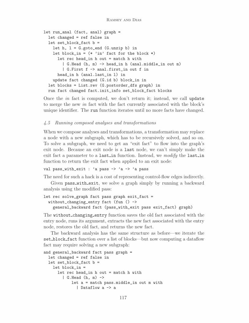
let run_anal (fact, anal) graph =

let changed = ref false in

let set_block_fact b =

let h, l = G.goto_end (G.unzip b) in

let block_in = (* ’in’ fact for the block *)

let rec head_in h out = match h with

| G.Head (h, m) -> head_in h (anal.middle_in out m)

| G.First f -> anal.first_in out f in

head_in h (anal.last_in l) in

update fact changed (G.id b) block_in in

let blocks = List.rev (G.postorder_dfs graph) in

run fact changed fact.init_info set_block_fact blocks

Once the in fact is computed, we don’t return it; instead, we call updateto merge the new in fact with the fact currently associated with the block’sunique identifier. The run function iterates until no more facts have changed.

4.5 Running composed analyses and transformations

When we compose analyses and transformations, a transformation may replacea node with a new subgraph, which has to be recursively solved, and so on.To solve a subgraph, we need to get an “exit fact” to flow into the graph’sexit node. Because an exit node is a last node, we can’t simply make theexit fact a parameter to a last in function. Instead, we modify the last in

function to return the exit fact when applied to an exit node:

val pass_with_exit : ’a pass -> ’a -> ’a pass

The need for such a hack is a cost of representing control-flow edges indirectly.

Given pass with exit, we solve a graph simply by running a backwardanalysis using the modified pass:

let rec solve_graph fact pass graph exit_fact =

without_changing_entry fact (fun () ->

general_backward fact (pass_with_exit pass exit_fact) graph)

The without changing entry function saves the old fact associated with theentry node, runs its argument, extracts the new fact associated with the entrynode, restores the old fact, and returns the new fact.

The backward analysis has the same structure as before—we iterate theset block fact function over a list of blocks—but now computing a dataflowfact may require solving a new subgraph:

and general_backward fact pass graph =let changed = ref false inlet set_block_fact b =let block_in =

let rec head_in h out = match h with| G.Head (h, m) ->

let a = match pass.middle_in out m with| Dataflow a -> a

117

Ramsey and Dias

| Rewrite g -> solve_graph fact pass g out inhead_in h a

| G.First f ->match pass.first_in out f with| Dataflow a -> a| Rewrite g -> solve_graph fact pass g out in

let h, l = G.goto_end (G.unzip b) inlet a = match pass.last_in l with| Dataflow a -> a| Rewrite g -> solve_graph fact pass g fact.init_info in

head_in h a inupdate fact changed (G.id b) block_in in

let blocks = List.rev (G.postorder_dfs graph) inrun fact changed fact.init_info set_block_fact blocks

This function never mutates a flow graph—rather, it computes the solutionto the dataflow equations as if the flow graph had been mutated.

To actually rewrite the graph, we require two steps: the first step calls thesolve graph function defined above, which iterates to a solution; the secondstep uses that solution to rewrite the graph.

let rec solve_and_rewrite fact pass graph exit_fact =

let a = solve_graph fact pass graph exit_fact in (* step 1 *)

let g = (* step 2 *)

backward_rewrite fact (pass_with_exit pass exit_fact) graph in

a, g

The rewriting step is straightforward. Function rewrite blocks goes throughall the blocks, accumulating the rewritten graph. Rewriting a last node stripsthe entry node off the new graph, replacing the last node. Rewriting middle

and first nodes is done similarly, except that each new graph is spliced ontoan accumulating tail. Here is an excerpt from the code:

and backward_rewrite fact pass graph =

let rec rewrite_blocks rewritten fresh =

match fresh with

| [] -> rewritten

| b :: bs ->

let rec rewrite_next_block () =

let h, l = G.goto_end (G.unzip b) in

match pass.last_in l with

| Dataflow a -> propagate h a (G.Last l) rewritten

| Rewrite g ->

let a, g = solve_and_rewrite fact pass g fact.init_info in

let t, g = G.remove_entry g in

let rewritten = Unique.Map.union g rewritten in

propagate h a t rewritten

and propagate : G.head -> ’a -> G.tail -> G.graph -> G.graph =

... similar code for middle and first nodes ...

rewrite_next_block () in

rewrite_blocks Unique.Map.empty (List.rev (G.postorder_dfs graph))

118

Ramsey and Dias

Because new graphs proposed via Rewrite are not retained, such graphs maybe solved multiple times as dataflow iterates. As shown in Section 5, however,this does not seem to be much of a problem in practice—perhaps becausemost rewrites are small. A typical rewrite replaces one machine instructionwith another or deletes an instruction by rewriting it to the empty graph.

4.6 The full implementation

For clarity, the code above has been simplified in two ways:

• The full implementation threads an integer “transaction limit,” which isused to cap the number of rewrites permitted. The transaction limit, whichis global to the entire compilation, is used to isolate bugs (Whalley 1994):by doing binary search on the limit, our test scripts can quickly find theexact transformation that turns good code into bad code.

• The full implementation also threads a Boolean that tells the compiler driverwhether this particular pass did any rewriting. Rewriting in one pass maycause the driver to run another pass; for example, if our peephole optimizersuccessfully rewrites instructions, we run another pass of dead-assignmentelimination.

The code we omitted does only bookkeeping; all the real work is shown above.

The complete implementation of the dataflow engine is about 425 linesof ML, broken down as follows:

40 lines Type definitions and module abbreviations

80 lines Functions for composing analyses and transformations

75 lines Utility functions, including run and update

90 lines Backward dataflow functions generalizing those shown above

90 lines Similar forward dataflow functions not shown in this paper

50 lines Debugging support

5 Performance

Compared with an imperative data structure, an applicative data structurerequires more frequent allocation and more copying, so it might be slower;but the objects allocated are smaller and shorter-lived, so it might be faster.To learn the actual effect on performance, we measured compile times andmemory allocation on three sets of benchmarks: code generated from C bythe lcc compiler (Fraser and Hanson 1995), code generated from ML by ML-ton (Cejtin et al. 2004), and code generated from Java bytecodes by Whirl-wind. Table 1 summarizes the results. The applicative flow graph actuallyperforms a bit better than its imperative counterpart; Table 1 shows the im-provement across each benchmark suite, as well as the range of improvementsfor individual benchmarks.

119

Ramsey and Dias

Front end(# benchmarks)

Range ofLine Counts

Compile-timeratios

(applicative /imperative)

Allocationratios

(applicative /imperative)

Source C-- Total Range Total Range

lcc (14) 17–137 93–543 0.87 0.81–0.89 1.03 1.00–1.05

MLton (32) 12–6,668 2,738–142,966 0.71 0.46–0.87 0.91 0.86–1.02

Whirlwind (3) n/a 11,662–39,025 0.90 0.82–0.92 0.98 0.96–1.01

Table 1Performance improvements of the zipper control-flow graph

The measurements in Table 1 reflect costs with optimization turned off.With optimization turned on, it is hard to make an apples-to-apples com-parison: the old optimizer uses a dataflow framework that does not composeanalyses and transformations; some of the older optimizations are more con-servative than the newer ones; and some of the older optimizations run onceinstead of being iterated to a fixed point. Still, when we compensate for thesedifferences as best we can, the results are similar: the applicative flow graphperforms about 10% better than its imperative counterpart.

6 Discussion

6.1 Differences in programming

Aside from overall simplification, the main benefit of the new flow graph isthat client code can tell statically when a node may have multiple inedges ormultiple outedges. This knowledge has been most helpful in our register allo-cators, which maintain information about the register or stack slot in whicheach source-language variable is placed. In the old flow graph, informationwas associated with each node using a finite map; we put the information ineach node because we didn’t know the number of edges statically. In the newflow graph, we know at compile time where the fork and join points are, andit is easy and natural to store the variable information in the property listsassociated with each basic block. This change leads to other simplificationswhich ultimately reduce the compiler’s memory requirements. It is certainlypossible to do things efficiently using the old flow graph; once we understoodwhat was going on, we back-ported the improvements to the old register al-locator, in order to make fairer comparisons in Section 5. What’s interestingis that the new flow graph led us to write code that was not just simpler butalso more efficient.

120

Ramsey and Dias

6.2 Alternatives in representation

When we “zip” a block, we put it into the normal form first * tail. Wecould as easily have chosen head * last, but first * tail is more convenientfor construction. The bad property of these normal forms is that they arebiased; first * tail is more efficient for algorithms that walk the flow graphforward, but head * last is more efficient for backward algorithms. We caneasily change forms by using the goto start and goto end functions, buteach of these functions costs linear time and allocation per use. An intriguingalternative would be to store blocks in the form head * tail. We could thenmake forward bias or backward bias a dynamic property of the graph. Inparticular, we could backward-bias the graph before running several different,consecutive backward algorithms, thereby amortizing the time and allocationrequired.

6.3 Experience and conclusion

When we decided to abandon our imperative control-flow graph, we fearedthere would be a performance cost for frequent zipping and unzipping, but wehoped for a simplification that would be worth any costs. We were pleasantlysurprised to learn our applicative flow graph outperforms the imperative ver-sion. And the gain in simplicity has been everything we hoped for: the flowgraph itself is much simpler, we have more confidence in the code, and theclients are either significantly simpler or mostly unchanged. We have beenespecially pleased with the compositional dataflow-solving framework, whichwe had always wanted to build but had been afraid to tackle using the imper-ative flow graph. We expect that the applicative control-flow graph based onHuet’s zipper will serve us for a long time to come, and we hope it will serveothers as well.

Acknowledgement

Matthew Fluet told us about the internals of MLton, and Simon Peyton Jonesgave us a tour of GHC. Christian Lindig built the first n versions of thecontrol-flow graph. Greg Morrisett asked good questions and encouraged usto publish. The anonymous referees made a number of helpful suggestions.

This work has been supported by NSF grants CCR-0096069 and ITR-0325460 and by an Alfred P. Sloan Research Fellowship.

References

Andrew W. Appel. 1998. Modern Compiler Implementation. Cambridge UniversityPress, Cambridge, UK. Available in three editions: C, Java, and ML.

121

Ramsey and Dias

Manuel E. Benitez and Jack W. Davidson. 1988 (July). A portable global optimizerand linker. Proceedings of the ACM SIGPLAN ’88 Conference on ProgrammingLanguage Design and Implementation, in SIGPLAN Notices, 23(7):329–338.

Manuel E. Benitez and Jack W. Davidson. 1994 (March). The advantages ofmachine-dependent global optimization. In Jurg Gutknecht, editor, ProgrammingLanguages and System Architectures, volume 782 of Lecture Notes in ComputerScience, pages 105–124. Springer Verlag.

Henry Cejtin, Matthew Fluet, Suresh Jagannathan, and Stephen Weeks.2004 (December). The MLton Standard ML compiler. See slides athttp://mlton.org/Talk.

Christopher W. Fraser and David R. Hanson. 1995. A Retargetable C Compiler:Design and Implementation. Benjamin/Cummings, Redwood City, CA.

Gerard Huet. 1997 (September). The Zipper. Journal of Functional Programming,7(5):549–554. Functional Pearl.

R. John Muir Hughes. 1986 (March). A novel representation of lists and its appli-cation to the function “reverse”. Information Processing Letters, 22(3):141–144.

Jens Knoop, Dirk Koschutzki, and Bernhard Steffen. 1998. Basic-block graphs:Living dinosaurs? In Kai Koskimies, editor, Compiler Construction (CC’98),pages 63–79, Lisbon. Springer LNCS 1383.

Donald E. Knuth. 1981. Seminumerical Algorithms, volume 2 of The Art of Com-puter Programming. Addison-Wesley, Reading, MA, second edition.

Sorin Lerner, David Grove, and Craig Chambers. 2002 (January). Composingdataflow analyses and transformations. Conference Record of the 29th AnnualACM Symposium on Principles of Programming Languages, in SIGPLAN No-tices, 31(1):270–282.

Simon L. Peyton Jones. 1992 (April). Implementing lazy functional languages onstock hardware: The spineless tagless G-machine. Journal of Functional Pro-gramming, 2(2):127–202.

Simon L. Peyton Jones, Norman Ramsey, and Fermin Reig. 1999 (September). C--:a portable assembly language that supports garbage collection. In InternationalConference on Principles and Practice of Declarative Programming, volume 1702of LNCS, pages 1–28. Springer Verlag.

Norman Ramsey and Jack W. Davidson. 1998 (June). Machine descriptions tobuild tools for embedded systems. In ACM SIGPLAN Workshop on Languages,Compilers, and Tools for Embedded Systems (LCTES’98), volume 1474 of LNCS,pages 172–188. Springer Verlag.

Norman Ramsey and Simon L. Peyton Jones. 2000 (May). A single intermedi-ate language that supports multiple implementations of exceptions. Proceedingsof the ACM SIGPLAN ’00 Conference on Programming Language Design andImplementation, in SIGPLAN Notices, 35(5):285–298.

David B. Whalley. 1994 (September). Automatic isolation of compiler errors. ACMTransactions on Programming Languages and Systems, 16(5):1648–1659.

122