an information-theoretic analysis of grover's …

AN INFORMATION-THEORETIC ANALYSIS OFGROVER'S ALGORITHM

Erdal ArikanElectrical-Electronics Engineering Department,

Silkent University, 06533 Ankara, Turkey

[email protected]

Abstract Grover discovered a quantum algorithm for identifying a target element in anunstructured search universe of N items in approximately 1r/4VN queries to aquantum oracle. For classical search using a classical oracle, the search complexity is of order N /2 queries since on average half of the items must be searched.In work preceding Grover's, Bennett et al. had shown that no quantum algorithmcan solve the search problem in fewer than D(VN) queries. Thus, Grover'salgorithm has optimal order of complexity. Here, we present an informationtheoretic analysis of Grover's algorithm and show that the square-root speed-upby Grover's algorithm is the best possible by any algorithm using the same quantum oracle.

Keywords: Grover's algorithm, quantum search, entropy.

1. Introduction

Grover [1], [2] discovered a quantum algorithm for identifying a target element in an unstructured search universe of N items in approximately 1r/ 4vNqueries to a quantum oracle oracle. For classical search using a classical oracle,the search complexity is clearly oforderN /2 queries since on average halfoftheitems must be searched. It has been proven that this square-root speed-up is thebest attainable performance gain by any quantum algorithm. In work precedingGrover's, Bennett et al. [4] had shown that no quantum algorithm can solvethe search problem in fewer than O(vN) queries. Following Grover's work,Boyer et al. [5] showed that Grover's algorithm is optimal asymptotically, andthat square-root speed-up cannot be improved even if one allows, e.g., a 50%probability of error. Zalka [3] strengthened these results to show that Grover'salgorithm is optimal exactly (not only asymptotically). In this correspondencewe present an information-theoretic analysis of Grover's algorithm and showthe optimality of Grover's algorithm from a different point of view.

339

A.S. Shumovsky and v.1. Rupasov (eds.), Quantum Communication and Information Technologies. 339-347.© 2003 Khtwer Academic Publishers.

340 QUANTUM COMMUNICATION AND INFORMATION TECHNOLOGIES

2. A General Framework for Quantum Search

Weconsider the following general framework for quantum search algorithms.We let X denote the state of the target and Y the output of the search algorithm.We assume that X is uniformly distributed over the integers 0 through N - 1.Y is also a random variable distributed over the same set of integers. Theevent Y = X signifies that the algorithm correctly identifies the target. Theprobability of error for the algorithm is defined as Pe = P(Y =1= X).The state of the target is given by the density matrix density matrix

N-l

PT = L (l/N)lx)(xl,x=o

(1)

where {Ix)} is an orthonormal set. We assume that this state is accessible to thesearch algorithm only through calls to an oracle oracle whose exact specificationwill be given later. The algorithm output Y is obtained by a measurementperformed on the state of the quantum computer at the end of the algorithm.We shall denote the state of the computer at time k = 0,1, ... by the densitymatrix pc(k). We assume that the computation begins at time 0 with the stateof the computer given by an initial state pc(O) independent of the target state.The computer state evolves to a state of the form

N-l

pc(k) = L (l/N)Px(k)x=o

(2)

at time k, under the control of the algorithm. Here, Px (k) is the state of thecomputer at time k, conditional on the target value being x. The joint state ofthe target and the computer at time k is given by

N-l

PTc(k) = L (l/N)lx)(xl ® Px(k).x=o

(3)

The target state (1) and the computer state (2) can be obtained as partial tracesof this joint state.We assume that the search algorithm consists of the application of a sequence

of unitary operators on the joint state. Each operator takes one time unit to complete. The computation starts at time 0 and terminates at a predetermined timeK, when a measurement is taken on pc(K) and Y is obtained. In accordancewith these assumptions, we shall assume that the time index k is an integer inthe range 0 to K, unless otherwise specified.There are two types of unitary operators that may be applied to the joint state

by a search algorithm: oracle oracle and non-oracle. A non-oracle operator is

Analysis ofGrover's algorithm

of the form I @ U and acts on the joint state as

341

PTc(k + 1) = (I @ U) PTc(k) (I @ U)t = 2.)ljN) Ix) (xl @ UPx(k)Ut.x

(4)

Under such an operation the computer state is transformed as

pc(k + 1) = Upc(k)Ut. (5)

Thus, non-oracle operators act on the conditional states Px (k) uniformly; Px (k+1) = UPx (k) ut. Only oracle oracle operators have the capability of acting onconditional states non-uniformly.An oracle operator is of the form L:x Ix) (xl @ Ox and takes the joint state

PTc(k) to

PTc(k + 1) = 2.)ljN)lx)(xl @ OxPx(k)Ol·x

The action on the computer state is

pc(k + 1) = 2.)ljN)OxPx(k)Ol.x

(6)

(7)

All operators, involving an oracle or not, preserve the entropy entropy of thejoint state PTc(k). The von Neumann entropy Von Neumann entropy of thejoint state remains fixed at S[PTc(k)] = log N throughout the algorithm. Nonoracle operators preserve also the entropy of the computer state; the action (5)is reversible, hence S[pc(k + 1)] = S[pc(k)]. Oracle action on the computerstate (7), however, does not preserve entropy; S [pc(k + 1)] =1= S [pc(k)], ingeneral.Progress towards identifying the target is made only by oracle oracle calls

that have the capability of transferring information from the target state to thecomputer state. We illustrate this information transfer in the next section.

3. Grover's Algorithm

Grover's algorithm can be described within the above framework as follows.The initial state of the quantum computer is set to

where

pc(Q) = Is) (sl

N-l

Is) = L (ljvN)lx).x=o

(8)

(9)


Since the initial state is pure, the conditional states Px (k) will also be pure forall k 2: 1.Grover's algorithm uses two operators: an oracle operator with

Ox = I - 2Ix)(xl, (10)

and a non-oracle operator (called 'inversion about the mean') given by I @ Uswhere

Us = 2Is)(sl- I. (11)

Both operators are Hermitian.Grover's algorithm interlaces oracle calls with inversion-about-the-mean op

erations. So, it is convenient to combine these two operations in a single operation, called Grover iteration, by defining Gx = UsOx . The Grover iterationtakes the joint state PTe (k) to

PTc(k + 1) = 2)I/N)lx)(xl @ GxPx(k)Gtx

(12)

In writing this, we assumed, for notational simplicity, thatGx takes one time unitto complete, although it consists of the succession of two unit-time operators.Grover's algorithm consists of K = (1r/ 4)VN successive applications of

Grover's iteration beginning with the initial state (8), followed by a measurement on pc(K) to obtain Y. The algorithm works because the operatorGx canbe interpreted as a rotation ofthe x-s plane by an angle B= arccos(l- 2/N) ~2/VN radians. So, in K iterations, the initial vector Is), which is almost orthogonal to Ix), is brought into alignment with Ix).Grover's algorithm lends itself to exact calculation of the eigenvalues of

Pc(k), hence to computation of its entropy. The eigenvalues of Pc(k) are

of multiplicity 1, and

A (k) = sin2 (Bk)2 N-l

of multiplicity N - 1. The entropy of Pc(k) is given by

(13)

(14)

and is plotted in Fig. 1 for N = 220 . (Throughout the paper, the unit of entropyis bits and log denotes base 2 logarithm.) The entropy S(Pc(k)) has period1r/B ~ (1r/2)VN.Our main result is the following lower bound on time-complexity.

Analysis ofGrover's algorithm 343

20 .-------.-----,........,....----.------.------.----~..__--____,,._--____,

18

16

14

122'e~10ecUJ

8

6

4

2

500 1000 1500 2000No. of Grover iterations

2500 3000 3500

Figure 1. Evolution of entropy in Grover's algorithm.

Proposition 1 Any quantum search algorithm that uses the oracle calls {Ox}as defined by (10) must call the oracle at least

(l-P 1) r;;:;K> __e+ vN

- 21f 1f logN(16)

times to achieve a probability oferror Pe.

For the proof we first derive an information-theoretic inequality. For anyquantum search algorithm of the type described in section 2, we have by Fano'sinequality,

H(YIX) :s; H(Pe ) + Pe log(N - 1) :s; H(Pe ) + Pe log(N), (17)

where for any 0 :s; u :s; 1

H(u) = -5log5 - (1- 5)log(1- 5). (18)


On the other hand,

H(XIY) H(X) - I(X; Y)

10gN - I(X;Y)

> logN - S(pc(K)) (19)

where in the last line we used Holevo's bound [6, p. 531].Let J-lk be the largest eigenvalue (sup-norm) of pc(k). We observe that

J-lk begins at time °with the value 1 and evolves to the final value J-lK at thetermination of the algorithm. We have

S(pc(K))

-J-lK log J-lK - (1 - J-lK) log[(1 - J-lK )/(N - 1)] (20)

1i(J-lK) + (1 - J-lK) log N. (21)

since the entropy entropy is maximized, for a fixed J-lK, by setting the remainingN - 1 eigenvalues equal to (1 - J-lK)/(N - 1). Combining (19) and (21),

J-lK logN :S Pe log N +1i(Pe ) + 1i(J-lK) :S Pe logN + 2 (22)

Now, let

~ = SUp{lJ-lk+l - J-lkl : k = 0,1, ... ,K -I}. (23)

This is the maximum change in the sup norm of pc(k) per algorithmic step.Clearly,

1 - J-lKK? ~ .

Using the inequality (22), we obtain

K1 - Pe + 2/ log N> .

- ~(24)

Thus, any upper bound on ~ yields a lower bound on K. The proof will becompleted by proving

Lemma 1 ~ :S 2Jr/ VN.We know that operators that do not involve oracle calls do not change the

eigenvalues, hence the sup norm, of pc(k). So, we should only be interestedin bounding the perturbation of the eigenvalues of pc(k) as a result of anoracle call. We confine our analysis to the oracle operator (10) that the Groveralgorithm uses.


For purposes of this analysis, we shall consider a continuous-time representation for the operatorOx so that we may break the action ofOx into infinitesimaltime steps. So, we define the Hamiltonian

H x = - 1f lx)(xl

and an associated evolution operator

Ox(T) = e-iTHx = 1+ (ei1rT- 1)lx)(xl.

The operator Ox is related to Ox(T) by Ox = Ox(1).We extend the definition of conditional density to continuous time by

Px(ko+ T) = Ox(T)Px(ko)Ox(T)t

for 0 :S T :S 1. The computer state in continuous-time is defined as

x

(25)

(26)

(27)

Let {An(t), un(t)}, n = 1, ... ,N, be the eigenvalues and associated normalized eigenvectors of pc(t). Thus,

pc(t)lun(t)) = An(t)lun(t)), (un(t)lpc(t) = An(t)(un(t)l,

(un(t)lum(t)) = on,m. (28)

Since pc(t) evolves continuously, so do An(t) and un(t) for each n.Now let (A (t), u (t)) be anyone of these eigenvalue-eigenvector pairs. By a

general result from linear algebra (see, e.g., Theorem 6.9.8 ofStoer and Bulirsch[7, p. 389] and the discussion on p. 391 of the same book),

d~~t) = (u(t)ldP~/t) lu(t)). (29)

dA(t)dt

To see this, we differentiate the two sides ofthe identity A(t) = (u(t)lpc(t)lu(t)),to obtain

(u'(t)lpc(t)lu(t)) + (u(t)ldP~?) lu(t)) + (u(t)lpc(t)lu'(t))

(u(t)ldP~/t) lu(t)) + A(t)[(u'(t)lu(t)) + (u(t)lu'(t))]

(u(t)ldP~?) lu(t)) + A(t) :t (u(t)lu(t))

(u(t)ldp~?) lu(t))

where the last line follows since (u(t)lu(t)) = 1.


Differentiating (27), we obtain

dpc(t) ~ .dt = L..- -(z/N)[Hx,Px(t)]

x

(30)

where [".] is the commutation operator. Substituting this into (29), we obtain

Id~~t) I

<

(u(t)l- ~ L[Hx,Px(t)] lu(t))x

2N L(u(t)IHxPx(t)lu(t))

x

(a) 2< N L(u(t)IH;lu(t)) L(u(t)lpi(t)lu(t))

x x

(b) 2

NL 1T2 1(u(t)lx)12 y'N(u(t)lpc(t)lu(t))

x

<

21T 1""\77\VIV 1· V A(t)

21T

VIV

(31)

where (a) is the Cauchy-Schwarz inequality, (b) is due to (i) p;(t) = Px(t) asit is a pure state, and (ii) the definition (27). Thus,

11kO

+l dA(t) IIA(ko+ 1) - A(ko)1 = -dt :s; 21T/vN.ko dt

Since this bound is true for any eigenvalue, the change in the sup norm ofPc (t)is also bounded by 21T/ VIV.

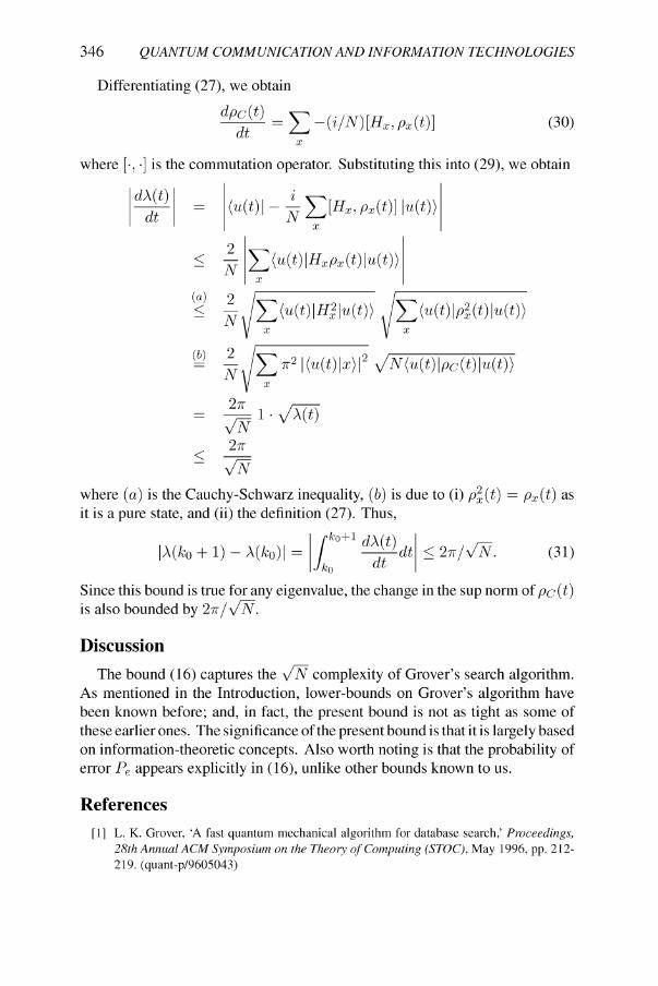
Discussion

The bound (16) captures the VIV complexity of Grover's search algorithm.As mentioned in the Introduction, lower-bounds on Grover's algorithm havebeen known before; and, in fact, the present bound is not as tight as some ofthese earlier ones. The significance ofthe present bound is that it is largely basedon information-theoretic concepts. Also worth noting is that the probability oferror Pe appears explicitly in (16), unlike other bounds known to us.

References[1] L. K. Grover, 'A fast quantum mechanical algorithm for database search,' Proceedings,

28th Annual ACM Symposium on the Theory ofComputing (STOC), May 1996, pp. 212219. (quant-p/9605043)


[2] L. K. Grover, 'Quantum mechanics helps in searching for a needle in a haystack,' Phys.Rev. Letters, 78(2),325-328, 1997. (quant-ph/9605043)

[3] C. Zalka, 'Grover's quantum searching is optimal,' Phys. Rev. A, 60,2746 (1999). (quantph/9711070v2)

[4] C. H. Bennett, E. Bernstein, G. Brassard, and U. V. Vazirani, 'Strength and weaknessesof quantum computing,' SIAM Journal on Computing, vol. 26, no. 5, pp. 1510-1523, Oct.1997. (quant-ph/9701001)

[5] M. Boyer, G. Brassard, P. Hoeyer, and A. Tapp, 'Tight bounds on quantum computing,'Proceedings 4th Workshop on Physics and Computation, pp. 36-43, 1996. Also Fortsch.Phys. 46(1998) 493-506. (quant-ph/9605034)

[6] M.A. Nielsen and I.L. Chuang, Quantum Computation and Quantum Information, Cambridge University Press, 2000.

[7] J. Stoer and R. Bulirsch, Introduction to Numerical Analysis. Springer, NY: 1980.

an information-theoretic analysis of grover's …

Documents