50 100 150 200 250 300 350 400 450-40

-30

-20

-10

0

10

20

30

40

50

Range gates

Pow

er, d

B

Svetlana Bachmann

February 2004

-40 -20 0 20 40-60

-40

-20

0

20

40

60

Velocity (ms-1)

Pow

er (d

B)

in front ofairplanebehindclear air

S.Bachmann

S.Bachmann

-40 -20 0 20 40-60

-50

-40

-30

-20

-10

0

10FFT

Velocity (ms-1)

Powe

r (dB

)

Analysis of Doppler spectra obtained with WSR-88D radar from non-stormy environment

National Oceanic and Atmospheric Administration National Severe Storm Laboratory Norman, Oklahoma

University Of Oklahoma Cooperative Institute for

Mesoscale Meteorological Studies

UNIVERSITY OF OKLAHOMA

GRADUATE COLLEGE

ANALYSIS OF DOPPLER SPECTRA OBTAINED WITH

WEATHER RADAR IN NON STORMY ENVIRONMENT

A THESIS

SUBMITTED TO THE GRADUATE FACULTY

In partial fulfillment of the requirements for the

degree of

MASTER OF SCIENCE

By

SVETLANA MONAKHOVA BACHMANN Norman, Oklahoma

2004

©Copyright by SVETLANA MONAKHOVA BACHMANN 2004 All Rights Reserved

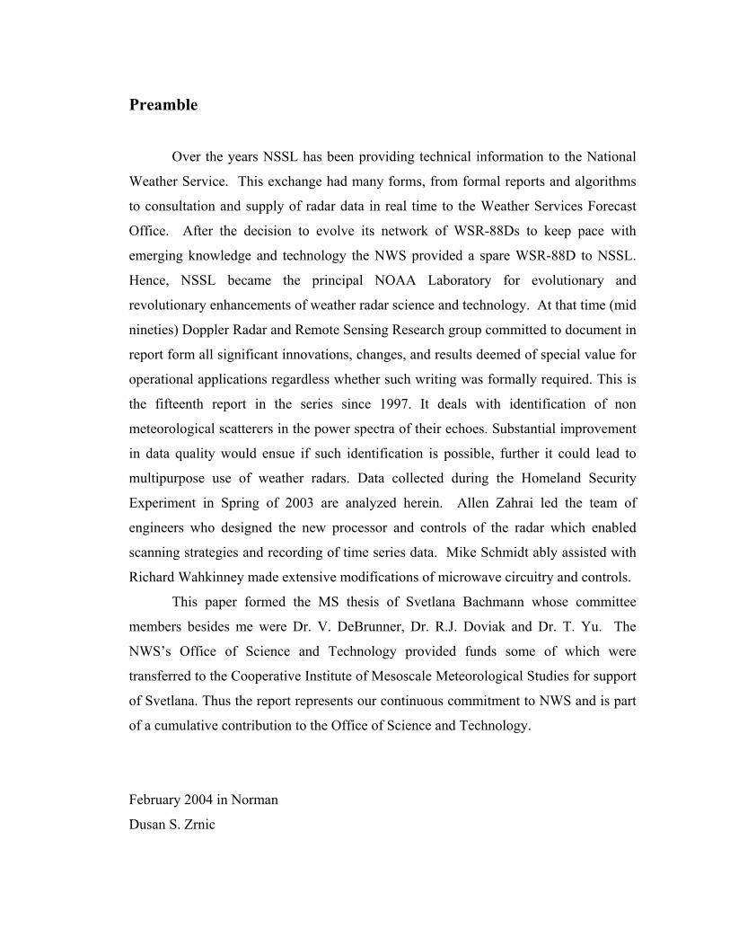
Preamble

Over the years NSSL has been providing technical information to the National

Weather Service. This exchange had many forms, from formal reports and algorithms

to consultation and supply of radar data in real time to the Weather Services Forecast

Office. After the decision to evolve its network of WSR-88Ds to keep pace with

emerging knowledge and technology the NWS provided a spare WSR-88D to NSSL.

Hence, NSSL became the principal NOAA Laboratory for evolutionary and

revolutionary enhancements of weather radar science and technology. At that time (mid

nineties) Doppler Radar and Remote Sensing Research group committed to document in

report form all significant innovations, changes, and results deemed of special value for

operational applications regardless whether such writing was formally required. This is

the fifteenth report in the series since 1997. It deals with identification of non

meteorological scatterers in the power spectra of their echoes. Substantial improvement

in data quality would ensue if such identification is possible, further it could lead to

multipurpose use of weather radars. Data collected during the Homeland Security

Experiment in Spring of 2003 are analyzed herein. Allen Zahrai led the team of

engineers who designed the new processor and controls of the radar which enabled

scanning strategies and recording of time series data. Mike Schmidt ably assisted with

Richard Wahkinney made extensive modifications of microwave circuitry and controls.

This paper formed the MS thesis of Svetlana Bachmann whose committee

members besides me were Dr. V. DeBrunner, Dr. R.J. Doviak and Dr. T. Yu. The

NWS’s Office of Science and Technology provided funds some of which were

transferred to the Cooperative Institute of Mesoscale Meteorological Studies for support

of Svetlana. Thus the report represents our continuous commitment to NWS and is part

of a cumulative contribution to the Office of Science and Technology.

February 2004 in Norman

Dusan S. Zrnic

iv

Acknowledgments

Many people have been of assistance in various parts of this project. My

advisor Dr. Victor DeBrunner taught me to be hard-working and willful in a struggle for

a solution. Dr. Dusan Zrnic’s contribution is invaluable in this work, and I

acknowledge him for his important ideas, discussions, and for directing me to the paths

leading to the solutions. His energy inspired new ideas.

I also acknowledge the advice of Dr. Tian-You Yu and I appreciate his

supportive, time-consuming review of my work. I am thankful for fruitful discussions

with Dr. Dick Doviak. I acknowledge Dr. Sebastian Torres and Chris Curtis for sharing

their experience in radar data acquisition and Matlab radar data processing. I value help

of NSSL senior software engineers David Priegnitz and Dan Suppes for their help with

the radar analysis tool, and the radar data. I appreciate the time and participation of

Donald Burges, NSSL Assistant Director Chief in Warning Research and Development

Division.

This work was performed while I was a graduate research assistant at the

Cooperative Institute for Mesoscale Meteorological Studies (CIMMS). Finding was

provided by the NWS Office of Science and Technology under the Nexrad Program

Improvement theme. Further data collection was supported by the National Severe

Storms Laboratory/NOAA and U.S. Army Biological and Chemical Defense Systems

(U.S. Dept. of Defense). I enjoyed working at National Severe Storm Laboratory

(NSSL) with all the nice and supportive people who work there. My great appreciation

is to CIMMS, NSSL, and OU School of Electrical and Computer Engineering.

I want to thank my daughter Kristina for allowing me to work on this project.

v

Contents 1. Introduction 1

1.1 Motivation 1 1.2 Radar Background 2 1.3 Clear-air 5 1.4 Ground Clutter 7 1.5 Literature review 7

2. Data Acquisition 9 2.1 Radar 9 2.2 Data Collection and Selection 10 2.3 Conversion into MATLAB 11

2.3.1. Radar data file name notation 12 2.3.2. MATLAB data file name notation 12

2.4 Preprocessing 13 2.5 Data sets used in this work 14

2.5.1 Data sets 2/10, and 4/02 14 2.5.2 Data set 3/26 16 2.5.3 Data 5/08 19

3. Airplanes 20 3.1 Tracking 20 3.2 Speed estimation 24

3.2.1 Doppler shift and velocity of a target 24 3.2.2 Velocity of airplanes 25

3.3 Cross section of an airplane 28 3.4 Fitting cross section to Gaussian 34 3.5 Spectra 39 3.6 Modulation 43 3.7 Conclusion 47

4. Birds 48 4.1 Single Birds 48 4.1.1 Tracking and spectra 51 4.1.2. Cross section 51

4.1.3. Simulation 57 4.2 Multiple Birds from data set 3/26 62 4.3 Multiple Birds from data set 5/8 63 4.4 Conclusion 67

5. Ground Clutter 68 5.1 Tower from data 2/10 69 5.2 Tower from data 4/02 73 5.3 Summary on decoding results 76 5.4 Conclusion 78

vi

6. Concluding Remarks 79 6.1 Summary 79 6.1.1 Airplanes 80 6.1.2. Birds 80

6.1.3. Ground Clutter 81 6.2 Further work 81

Appendix Table A1: Data 2/10 84 Table A2: Data 4/02 85

Table A3: Summary for data 2/10 and 4/02. 86

vii

Abstract

This thesis provides support in defining potential improvements to Doppler weather

radar signal processing techniques by (1) understanding the characteristics of the non-weather

scatterers, and (2) adjusting received phase-coded signal phase. The echo from point scatterers

(airplanes and birds) in a non-stormy environment is investigated in the time and frequency

domains. Further, it is compared to model simulations to build a background for differentiating

these echoes from weather signals and to develop procedures for data censoring. The phase

coded echo from a stationary point scatterer is examined to determine uncertainties in radar

oscillator phase caused by the phase shifter in the WSR-88D radar. The phase shifter is part of

a circuit for automatic calibration of the receiver and will be used to generate systematic phase

codes for mitigating range velocity ambiguities.

1

1. Introduction

1.1. Motivation

Weather radars operated by the National Weather Service in the USA are joined

in a network to provide spatially and temporally continuous coverage over the whole

country. Advances in accuracy of radar signals would significantly improve the radar

and radar network performances. Detected signals are processed with many

assumptions to simplify interpretation of the echo and enhance features deemed

important for identifying significant and/or hazardous phenomena. The results of

interpretation are often based on previous observations and matched to the conceptual

models. I identify that as a fuzzy approach, creating a blurry picture that is missing

detailed information that could be important. There is always clutter in signals and it

distorts the purposeful component of the signal. Getting rid of clutter, or compensating

for the loss caused by clutter might be possible by applying appropriate filtering and

enhancing techniques. To decide on the type of techniques suitable for one case or

another it is necessary to accumulate information characterizing echoes and its behavior

due to known conditions. My motivation is to study particular details in the echo signal

with the goal of extracting more information that would help classify the echoes.

The primary goals of this research are: a) to acquire information from clear-air

echoes obtained with an S-band (2-5 GHz 15-8cm) radar; b) to understand echo

characteristics of point scatterers in clear-air; c) to create models simulating the echo;

and d) to improve the interpretation of radar data by aggregating the information

associated with the target solutions (the combination of range, azimuth, course, and

velocity at any time) and the spectral signatures of the echoes. This information may

2

help to advance the radar performance by improving its signal processing techniques,

and may assist in developing an approach for differentiating point scatterers. By

surveying the echo signal features in time and frequency domains, I attempted to

determine a physical principle that regulates the appearance of the echo signal and

influences it. I verified the nature of the target signature occurrence and confirmed it

mathematically. I investigated the behavior of the signals and characterized them.

1.2. Radar Background

The radar operator may either define a Volume Coverage Pattern (VCP) or

interact with the radar’s operating computer to define the scan characteristics. Many

different VCPs that involve different scan strategies and sampling techniques are

employed with the radars used for the meteorological observations. Examples of

variables defining the VCP are (1) elevation, the antenna angle above horizontal; (2)

antenna rotation rate in degrees per second; (3) Pulse Repetition Frequency (PRF); (4)

number of pulses (M) that are transmitted along each radial. Radar transmits a beam of

radio frequency energy in discrete pulses which propagate away from the radar antenna

at the speed of light. The scatterers backscatter energy so that some of it returns to the

radar. Radar pulse volume is defined by wavelength of the transmitted energy, the

shape and size of the radar antenna, and the transmitted pulse width. The radar

resolution volume determines the region in space that contributes most energy to the

returned signal. The radar used in this work is described in Section 2.1. The radar has a

narrow Gaussian-shaped beam pattern. Each pulse is mainly contained within a

truncated cone, as shown in Figure 1.1. The transmitted beam assumes maximum

power along the beam centerline. The half-power circle (Figure 1.1) is the locus of

3

points where the power of transmitted energy has decreased to one-half of the

maximum power. The collection of such circles for all ranges defines a core, which is

considered to effectively contain the radar beam. The beam-width is the angular width

of the radar beam subtended by this half-power core.

Figure 1.1: Radar beam geometry. The maximum power of the beam lies along its centerline. Conceptual half-power circle defines the beam-width. All of the transmitted pulses have the same duration. Pulse 1 has a greater volume than pulse 2 because it is farther away from the radar.

Pulsed transmission is used to obtain range and motion information of the

scatterer. Long pulses (4.7 µs) have more energy and can be used for probing scatterers

at farther ranges but at lower pulse repetition times (PRTs). Short pulses (1.57 µs) can

be transmitted at higher PRT and therefore are used to measure unambiguously larger

velocities. Typical weather radar transmits megawatts of peak power. After the pulses

(concentrated in a narrow beam) are transmitted the electromagnetic energy will be

absorbed, diffracted, refracted, and reflected. Reflected from scatterers energy

experiences additional absorption, refraction and reflection on the return trip back to the

receive antenna. Thus, when a pulse is backscattered from scatterers, only a fraction of

the transmitted power is incident on the receive antenna. The radar receiver is very

sensitive and is capable of receiving powers as small as 10–14 W. The received signals

are mixed with a reference signal of the intermediate frequency (57.6 MHz) and

Bea

m-w

idth

beam centerline

Pulse 1Pulse 2 half-power circle

4

amplified. The echo voltage V backscattered to the radar from a point scatterer has a

phase ψe with respect to the transmitted pulse. The phase ψe from a stationary scatterer

is time independent. If the distance between radar and scatterer changes, the phase also

changes, creating a phase shift called the Doppler shift. Positive Doppler shift,

corresponding to a negative radial velocity, indicates motion toward radar. Negative

Doppler shift, related to positive velocity, shows motion of scatterers away from the

radar.

The Doppler radar receiver has two synchronous detectors which detect in-phase

I and quadrature-phase Q components of the echo signal V. According to Euler’s

relation the echo voltage can be represented by a two-dimensional phasor diagram in a

complex plane (Figure 1.2). The successive values of I-Q samples are measured at

equally spaced time intervals creating a time-series sequence.

Figure 1.2: Phasor diagram. The Doppler radar receiver detects in-phase I and quadrature-phase Q components of the echo signal V. I is the real part of the echo voltage V, Q is the imaginary part of V, and ψ e is echo phase.

I-Q samples of backscattered energy at the same range location for a number of

pulses (M) specified by the VCP are processed to generate spectral moments of one

range location, as shown in Figure 1.3a. Collection of consecutive range gates makes a

Q = Im{V} V

ψe

I = Re{V}

5

radial. A radial of data may consist of either equally spaced I, Q samples, or spectral

moments (Figure 1.3b). A cut is defined as a scan at a fixed elevation. Cut consists of

many radials as shown in Figure 1.3c. Radar data usually include many cuts. Cuts can

be scanned with different or constant settings. For example, cuts shown in Figure 1.3d

are taken at different elevation angles. When nothing in the radar settings is changed

from cut to cut the scan is continuous. Several cuts make a data file according to the

VCP or other radar operator requirements.

1.3. Clear-air

Doppler shift allows creation of a picture of “traffic” within the atmosphere. The

atmosphere-traffic includes (1) motion of air-masses (winds, clouds, vapor, dust,

smoke, etc.), (2) interference from other radio equipment or the sun, (3) movement of

aircrafts (airplanes, helicopters, balloons), and (4) passive and/or active displacement of

biota (birds and airborne insects). I refer to the atmosphere free of clouds and

precipitation as clear-air. Throughout the development of weather radar technology and

science, radar echoes from non-precipitation sources have been referred to by several

different names: angel echoes and clear-air echoes. These can occur as isolated point

or small area scatterers, layers, or volumes of distributed scatterers. Clear-air echoes

can appear granular, spotty. Current and recent literature indicates a widely held belief

that the primary cause of clear-air echoes is biota. (For example: Campistron, 1975;

Wilson, 1994; Rogers et al., 1991; Rabin and Doviak, 1989, and many others). In clear-

air reflections can be caused by refractive index fluctuations, biota, aircrafts, and

ground clutter. Clear-air echoes caused by point scatterers, e.g., birds, airplanes and

ground clutter are investigated in this thesis.

6

Pulse → Range-Time #

1

2

3 • Radial • •

M (a) Sample-Time Range location

(b) Radial of spectral moments

Figure 1.3: I-Q samples make the data. (a) I-Q samples of backscattered energy for M pulses; (b) radial of spectral moments, (c) radials in a cut, (d) cuts in a VCP. Note that cuts could be taken at different elevation angles (as shown) or at the same elevation as defined by the VCP.

250 m

PRT

…1.6 µs

I or Q sample

Radial

Cut 2

Cut 3

VCP

Cut 1

Cut 4

Cut

(c) (d)

7

1.4. Ground Clutter

Ground clutter is the return from obstacles on the ground. The returns from

ground scatterers are usually very large with respect to other echoes, and so can be

easily recognized (Accu-Weather NEXRAD Dopplar Radar Information Guide, 1995).

Ground-based obstacles may be immediately in the line of site of the main radar beam,

for instance hills, tall buildings, or towers. Alternatively, the returns may be from

objects, which although not directly within the field of view of the main radar beam, are

present within one of the side-lobes of the radar beam. In this case, even though the

side-lobe power is much lower than that of the main beam, the return may still be large

due to the closeness of the obstacle, and/or its large cross section.

Clutter is desired to be mitigated in order to improve the radar performance. For

weather radars, signals from biological scatterers, airplanes, and ground scatterers are

undesirable; the exception might be signals from passively transported insects which

map the motion of air. Contamination by birds is often a noisy signal covering entire

low elevation sites and preventing useful weather observations.

1.5. Literature Review

Echoes in clear-air have been documented from early days of radar meteorology

[16]. Birds have been implicated as sources of errors in wind profiling radars [14].

Even at close ranges, a narrow beam tracking radar can be affected by bird migration

[11]. Recognition of birds in the Doppler radar spectra of surveillance radars should be

possible from the beat frequency of the flapping wings [11], but this is not yet practical

[16]. Specialized spectral processing with associated recognition algorithms would

need to be developed [16].

8

The third base product of WSR-88D radars, Doppler spectrum width, has been

called “the largely ignored step child of Doppler weather radar” [7]. The actual number

of investigators regularly using radar to study birds has decreased significantly [11] due

to difficulty and costs of experiments [11].

There are no solutions to completely eradicate the range and velocity ambiguity

of weather echoes [10]. One of the approaches to reduce the ambiguities uses the

frequency domain to separate overlaid echoes and assign each one a correct range [17].

The random phase coding [17], systematic π/4 and π/2 phase coding [18], and

systematic SZ phase coding [10] techniques have been suggested for the recovery of

spectral parameters of the overlaid first- and second- trip echoes. I will examine the

phase coded echo from a stationary point scatterer to determine uncertainties in radar oscillator

phase caused by the phase shifter in the WSR-88D radar.

9

2. Data Acquisition

2.1 Radar

KOUN (Figure 2.1) is a research WSR-88D (Weather Surveillance Radar-88

Doppler) radar that is managed and operated by the National Severe Storms Laboratory.

The radar frequency is 2705 MHz. A WSR-88D system consists of the antenna,

pedestal, radome, tower, klystron transmitter, receiver, minicomputer, signal processor,

and radar product generator. The 10-cm wavelength (2.7-3.0 GHz) klystron transmitter

transmits with a nominal peak power output of 750 kW. The radar operates with either

short or long pulse. The short pulse-width of 1.57 µs is for pulse repetition

Figure 2.1: KOUN Doppler Radar WSR-88D used for data collection in this work.

10

frequencies (PRF) between 318 and 1304 Hz, and long pulse-width of 4.7 µsec is for

PRFs between 318 and 452 Hz. The parabolic antenna has a diameter of 8.5 m (27.9

ft), an antenna main-lobe one-way 3 dB beam-width of approximately 0.95°, and a first

side-lobe 27 dB below the main lobe. The signal transmitted by KOUN can be either

linear horizontal polarization or simultaneous horizontal/vertical polarization.

2.2. Data Collection and Selection

Time series data were collected using KOUN on the following dates: 12/11/2002,

2/10/2003, 04/02/2003, 26/03/2003, 05/08/2003. Data sets are described in section 2.5.

Data are reformatted and displayed on the prototype version of the Radar Analysis Tool

(RRAT), which is developed at NSSL. Figure 2.2 shows a typical display of RRAT

with plan-position indicator (PPI) on the right side, range-height indicator (RHI) on the

top left, and Spectral View window on the lower left. The PPI window of RRAT can

display velocity, reflectivity, or spectrum width with different zooming, color scale, and

a great variety of options under the tab property. The spectral view of RRAT can be

used to display the spectrum at a certain gate or in the gate with its 8 neighbors. The

RHI window cursor moves simultaneously with the PPI cursor, showing the location of

the gate in the vertical view of the radial and helping to estimate the 3-dimentional

location of the resolution volume. The tab Cut shows the changes of data with time,

animating the picture. This tool is a great help at browsing through a very large amount

of data quickly, but sufficient time is required for loading the data prior to using it.

Loading and processing the data may take tens of minutes depending on the size of the

radar data file, but processed data can be accessed instantly with a great variety of

displaying options. The RRAT was used to search for unusual spectra and unexplained

11

echoes, to get acquainted with the features of the data, and to choose interesting areas.

A list of file names, cut numbers, and the azimuth angles and ranges of the areas of

interest was recorded in order to keep track of and to prepare for extraction of the

radials containing those areas.

Figure 2.2: Example of the display of the Radar Analysis Tool (RRAT). Top-left: range-height indicator; lower-left: spectral view window; right-half plan-position indicator; most-right: color-scale bar. Middle spectrum is from the location, marked with the cursor on a highlighted white radial.

2.3 Conversion into MATLAB

The routine RaidRead was developed at NSSL for splitting a raw radar data file

into small portions of data and converting these into files of other formats, e.g.,

MATLAB format data files. A radar data file, consisting of a large number of radials

12

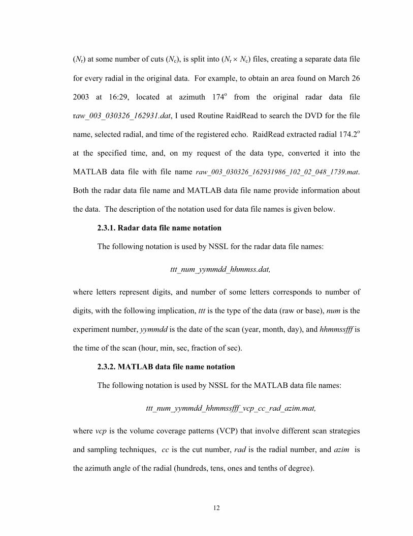
(Nr) at some number of cuts (Nc), is split into (Nr × Nc) files, creating a separate data file

for every radial in the original data. For example, to obtain an area found on March 26

2003 at 16:29, located at azimuth 174o from the original radar data file

raw_003_030326_162931.dat, I used Routine RaidRead to search the DVD for the file

name, selected radial, and time of the registered echo. RaidRead extracted radial 174.2o

at the specified time, and, on my request of the data type, converted it into the

MATLAB data file with file name raw_003_030326_162931986_102_02_048_1739.mat.

Both the radar data file name and MATLAB data file name provide information about

the data. The description of the notation used for data file names is given below.

2.3.1. Radar data file name notation

The following notation is used by NSSL for the radar data file names:

ttt_num_yymmdd_hhmmss.dat,

where letters represent digits, and number of some letters corresponds to number of

digits, with the following implication, ttt is the type of the data (raw or base), num is the

experiment number, yymmdd is the date of the scan (year, month, day), and hhmmssfff is

the time of the scan (hour, min, sec, fraction of sec).

2.3.2. MATLAB data file name notation

The following notation is used by NSSL for the MATLAB data file names:

ttt_num_yymmdd_hhmmssfff_vcp_cc_rad_azim.mat,

where vcp is the volume coverage patterns (VCP) that involve different scan strategies

and sampling techniques, cc is the cut number, rad is the radial number, and azim is

the azimuth angle of the radial (hundreds, tens, ones and tenths of degree).

13

2.4 Preprocessing

Each file with extension “.mat” consists of an array of complex data and a

header. A header is a structured array with description of the data. One radial of

MATLAB data has dimensions N×M, where N is the number of bins (range gates) and

M is the number of pulses. Each radial of data collected on 2/10, 4/02, and 3/26 has

dimensions 468×64, and a radial of data from 5/09 has dimensions 592×24.

After reading and plotting many radials (Figure 2.3), I selected the radials with

the most pronounced features, e.g., the strongest reflectivity for an airplane return,

andcreated collections or batches of data several radials in size for further processing.

50 100 150 200 250 300 350 400 450-40

-30

-20

-10

0

10

20

30

40

50

Range gates

Pow

er, d

B

airplane

Az=170.7

Time cut 11

Figure 2.3: Returned power along one radial. The echo from an airplane is indicated. High powers at close ranges are from ground clutter.

14

The radials for single birds were chosen as described in Section 4.1. The radials for

multiple birds were selected randomly (Section 4.3).

Most of the batches consist of neighboring or consecutive radials for several

reasons. First, the discrete nature of sampling suggests that a scatterer could be located

on the border of a sampling volume that would influence return from neighboring

locations. Second, a strong return signal could appear at the adjacent range gates due to

the spread of the range-dependent weighting function.

Figure 2.4 summarizes steps performed on a data file in the process of preparing

it for analysis. The purpose of data preparation is to allow the loading of data in

MATLAB with one command: load(‘filename’).

2.5 Data sets used in this work

2.5.1 Data sets from 2/10, and 4/02

The 2/10 and 4/02 data were obtained with a stationary antenna pointed at

azimuth 306° and elevation 0.3°, radiating with PRT 780 µs. Data were collected for

the Phase Shifter Test. One record of data consists of 468 consecutive (in range-time) I,

Q samples. Each radial has 64 records of such data (64 pulses × 468 ranges). A file of

data (raw_010_030210_165638.dat) consists of 100 radials (64 × 468 × 100). Both sets

include data collected with and without phase coding. There was no precipitation on

both dates. However the wind conditions were different: 3 ms-1 in February, and 10

ms-1 gusting to 15 ms-1 in April. This data is used in Chapter 5.

15

Figure 2.4: Data Preparation The time series data were collected by KOUN radar. Collected data stored on Raid (~130GB), read by ReadRaid to a workstation hard-drive, and archived on DVD/CD. The files of raw radar data were explored by means of Radar Analysis Tool. MATLAB data files were created with RaidRead. MATLAB data files were composed into batches of consecutive radials and prepared for analysis.

.mat file …

RaidRead Extraction of Radials Creation of MATLAB Files

.mat files

.dat file

List of radials

.

.

.

.dat files

Storage

Radar Analysis Tool

…

MATLAB Combining Radials into Batches

Radar KOUN

PC Ready Data Sets

Raid(~130 GB)

WS hard-drive

DVD/CD

Raid(~130 GB)

16

2.5.2 Data set from 3/26

The 3/26 data were obtained with an antenna scanning a sector at azimuth angles

150° through 190°. All data were collected with PRT 780 µs, at constant elevation 1.5°.

Data were collected for the Homeland Defense Radar Test.

There was no precipitation on March 26. I looked briefly at several hours of

data and did not have any particular reason to prefer one data file over another. Every

file consists of 20 time cuts 2.5 minutes long. A file (raw_003_030326_102921.dat)

with data collected from 10:29 until 10:32 was selected. Similar results were found

from the rest of files. Figure 2.5 shows reflectivity and velocity PPI of RRAT from one

time cut of the data.

a b Figure 2.5: One cut of data 3/26: (a) Reflectivity, (b) Velocity. Note that range rings here are 10 km apart.

17

PRT determines maximum unambiguous range and maximum unambiguous

velocity. Maximum unambiguous range Rmax is 117 km, calculated according to the

formula

Rmax = c Ts / 2, (2.7.1)

where c is the speed of light (c = 3×108 ms-1), Ts is PRT. Maximum unambiguous

velocity vmax is 32.05 m s-1, found according to the formula

vmax = PRT⋅4λ , (2.7.2)

where λ is the wavelength (λ = 10 cm).

Echoes from aircrafts, birds, insects, and ground clutter were expected in this

data set. Echoes found in this data are summarized in Table 2.1. Each row describes

the attributes of echoes found in the scan specified in column Range. The echo region

is described by its shape and values of its reflectivity (Z) and velocity (v). Assumption

on the type of echo is made according to its location (range) and description (shape,

reflectivity and velocity values simultaneously with the neighborhood evaluation).

Tracking several aircraft, I found the airplane flying for the Homeland Security Test. I

focus attention on this so-called Airplane-1, and another unknown Airplane-2 in

Chapter 3. Data with bird signatures is examined in Chapter 4.

Note that the category Airplanes in Table 2.1 includes a group Jet Airplanes.

The Jet Airplanes group can be differentiated because of the large velocities that could

be estimated from time-cut animation (tracking) and due to the high altitudes of these

strong point scatterers.

18

Table 2.1: Echoes in clear-air scan 3/26.

Echo Description Range

Shape Reflectivity and Velocity Assumption

Less then 5 km Area Z: high (20 to 40 dBZ)

v: zero

Ground Clutter: Buildings, Water-towers, Trees

Large area (most of the scan)

Z: below 0 dBZ v: in the range 0 to 5 ms-1

Wind blows toward the radar from south – south-east

Point Z: high (30 to 40 dBZ) v: zero

Ground Clutter: TV and Radio Towers

Less then 30 km

Point and small area

Z: weaker (less then 10 dBZ) v: with non-zero, and non-wind values Birds and Insects

15-30 km Point Z: 30-40 dBZ

v: a lot different from surroundings Airplanes

More then 30 km Point Z: 10-30 dBZ

v: non zero velocities Jet Airplanes

At different ranges

Point and small area

Z: weak (less then 10 dBZ) v: non-zero, and non-wind values Birds and Insects

2.5.3 Data set from 5/08

The data from 5/08 were obtained with a full 360° scan of rotating and rising

antenna. One file of data (raw_005_030509_015646.dat) consists of 14 cuts at different

elevation angles from 0.1° to 19.5° as shown in Table 2.2.

On 8 May 2003, after a tornadic super-cell, biological scatterers lighted up

KOUN displays for several hours between 2-5 UTC (9 May 2003). The time series data

files were taken at about 2 UTC on May 9 2003, or at 10 PM of May 8, local time.

19

Table 2.2: Elevation Angles and PRT of different cuts of data 5/08

Cut 0 1 2 3 4 5 6 7 8 9 10 11 12 13

Elevation,° .1 .5 1.5 2.5 3.5 4.5 5.5 6.5 7.5 8.7 10 12 14 19.5

PRT Long Short 986.67 µsec

The return from the birds would be easier to see from the pulses sent with short

PRT and at low elevation angle. Cut 03 is taken at the lowest elevation (2.5°) with

shorter PRT. The reflectivity PPI of cut 3 is shown in Figure 2.2. Maximum

unambiguous range Rmax is 148 km. Maximum unambiguous velocity vmax is 25.3 m s-1.

This data is analyzed in Chapter 4.

20

3. Airplanes

The track-while-scan (TWS) systems deployed on the military radars use the

combination of range, azimuth, course, and speed at any one time, known as the target's

solution, to predict possible location of the target at the next observation. During each

antenna sweep, the system attempts to correlate all returns with existing tracks. The

TWS systems may confuse two different targets if their tracks cross each other. This

motivated my research of the target signatures. The purpose of this chapter is to extract

information from the available radar data containing airplane echoes, with an intention

to discover a systematic structure in the echo spectra that possibly contains information

characterizing the airplane. The approach involved investigation of the reflectivity,

velocity, and spectra patterns of airplane returns, simulation of discovered features, and

verifying results by the actual available information. A main goal is to find

distinguishable features that can define an airplane signature and ultimately remove

these from weather echoes.

3.1 Tracking

Airplane-1 was flying in the center of the scanned sector at ranges from 9 to 15

km. It was moving north toward the radar at the time of cuts 0 through 15, then turned

east and started moving south, away from the radar. Airplane-2 entered the volume of

the scan from the west at the time of the 10th cut at a range of approximately 9 km and

kept flying north-west, gradually turning north, as shown in the radar trajectory Figure

3.1. The locations of the airplanes at different time cuts are tracked and given in the

columns Range and Azimuth of Table 3.1 for Airplane-1 and Table 3.2 for Airplane-2.

Both airplanes are at the same range about 10 km south from the radar during the 13th

21

Table 3.1: Reflectivity factors for Airplane-1

Cut

Time t

(h:m:s)

Target Range

r (km)

AzimuthAngle θ

(°)

Beam Height

h (m)

Reflec-tivity

Z (dBZ)

Equivalent Reflectivity

Ze (mm6m–3)

Reflectivity Per Volume

η×109

(mm6m–3m-4)

Cross sectionσb

(m2)

0 10:29:21 14.63 172.5 383 46.5 44668 127.13 0.9981 10:29:33 14.36 172.7 376 49.0 79433 226.06 1.7102 10:29:39 13.87 172.1 363 56.0 398107 1133.01 7.9953 10:29:48 13.60 172.7 356 47.5 56234 160.04 1.0864 10:29:56 13.12 171.7 343 50.5 112202 319.32 2.0165 10:30:03 12.86 172.3 337 48.5 70795 201.48 1.2226 10:30:10 12.59 171.3 329 44.5 28184 80.21 0.4667 10:30:19 12.10 171.9 317 44.0 25119 71.49 0.3848 10:30:26 11.87 171.0 310 49.5 89125 253.65 1.3119 10:30:34 11.63 171.4 304 43.0 19953 56.78 0.282

10 10:30:42 11.13 170.6 291 43.5 22387 63.71 0.29011 10:30:50 10.91 170.8 286 42.5 17783 50.61 0.22112 10:30:57 10.39 169.8 272 43.0 19953 56.78 0.22513 10:31:05 10.13 170.4 265 40.0 10000 28.46 0.10714 10:31:12 9.87 169.6 258 34.0 2512 7.15 0.02615 10:31:21 9.35 169.8 244 24.0 251 0.71 0.00216 10:31:28 9.36 167.3 245 35.0 3162 9.00 0.02917 10:31:36 9.60 166.6 251 40.5 11220 31.93 0.10818 10:31:43 9.87 165.8 258 42.0 15849 45.11 0.16119 10:31:50 10.35 167.4 271 46.0 39811 113.30 0.445

Table 3.2: Reflectivity factors for Airplane-2

Cut

Time t

(h:m:s)

Target Range

r (km)

AzimuthAngle θ

(°)

TargetHeight

h (m)

Reflec-tivity

Z (dBZ)

Equivalent Reflectivity

Ze (mm6m–3)

Reflectivity Per

Volume η×109

(mm6m–3m4)

Cross sectionσb

(m2)

8 10:30:26 9.6 190.2 251 42 15849 45.11 0.23310 10:30:42 9.91 187.7 259 44 25119 71.49 0.32511 10:30:50 9.95 188.2 260 39 7943 22.61 0.09912 10:30:57 10.2 184.6 267 58 630957 1795.69 7.11013 10:31:05 10.14 184.3 256 53 199526 567.85 2.13714 10:31:12 9.87 181.5 258 53 199526 567.85 2.02915 10:31:21 9.58 181.3 250 39 7943 22.61 0.07316 10:31:28 9.35 178.7 244 43 19953 56.78 0.18317 10:31:36 9.11 178.9 239 45 31623 90 0.30418 10:31:43 8.61 178.4 225 47 50119 142.64 0.51019 10:31:50 8.36 179.3 219 50 100000 284.6 1.118

22

time cut as indicated in Figures 3.2a and 3.2b. To track the airplanes the following

steps were performed. The position of the strong point reflectivity associated with non-

zero velocity at one time cut was noted. The next time cut was searched for a matching

point, which is assumed to be located at some range and azimuth angle close to the

location of previously registered point. The obtained points were connected as shown

in Figure 3.1, and the solid lines show the paths of airplanes as indicated. Numbers 0

through 19 near the data points show time cuts.

Figure 3.1: Trajectory of the airplanes. The radar is located above the figure. Axis range shows the distance from the radar. Airplane-1 is flying toward the radar for most of its path. Airplane-2 is turning. At the 13th time cut both airplanes are located at the same range. A 1° azimuth angle corresponds to 261.8 m at a range of 15 km, and to 157.1 m at 9 km range.

Range (km) Azimuth

(degree)

15

5

Airplane-2

10 Airplane-1

180 190 170 160 200

16 15 17 14 18 13 19 12 11 10 9 8 7

5 6 4

3 2 1 0

19 18 17 8 16 (9) 10 15 11 14 13 12

150

23

The oscillations in the paths of the airplanes in Figure 3.1 are likely due to the

backlash of the antenna that occurs during scanning a sector back and forth as opposed

to the full 360° scan. Backlash is caused by the lag in gears, servo mechanism and

encoders. The lag is not fully compensated, and hence shows as an offset between

azimuths obtained in clockwise and counter-clockwise motion. In some cases the

oscillations increased because of inaccurate reading of the data from the computer

screen (Figure 3.2). Data points 0 through 19 were read from reflectivity PPI, similar to

the one shown in Figure 3.2a. Every numbered point is associated with the center of the

highest reflectivity, estimated by eye, as explained in Figure 3.3. In this figure a part of

the reflectivity PPI with the Airplane-1 echo is magnified to show in detail pixels

corresponding to radar resolution volumes. One pixel is a rectangle 250 m long and

0.5° wide. Several pixels circled in Figure 3.3a show more than 30 dB reflectivity

a b Figure 3.2: 13th time cut of data 3/26 on the PPI of RRAT: (a) Reflectivity. (b) Velocity. Circles near 10 km range ring are used to show the locations of Airplane-1 and Airplane-2. Note that range rings here are 5 km apart.

Airplane-1

Airplane-2

Airplane-1

Airplane-2

24

Figure 3.3: Estimation of an airplane location from the reflectivity PPI. A part of reflectivity PPI with circled airplane echo, magnified to show gates in detail. The color-scale is the same as in Figure 3.2a. Pixels in the center of the circle have reflectivity values more then 40dBZ. The pixel to the right of center shows the largest value of reflectivity. Nevertheless, the center of the high reflectivity area is estimated to be the airplane location. It is done to avoid possible ground clutter and/or additional scatterer contamination values. Four adjacent pixels in a row have values more then 40 dB; therefore, this row

is likely to be the range of the airplane. Figure 3.3b shows that the pixel with highest

reflectivity (darkest color) is not in the center of the area. However, the center of the

area of high reflectivity values is estimated to be the azimuth angle of the airplane

location. The reading approximation introduces ±250 meters error.

3.2 Speed estimation

3.2.1 Doppler shift and velocity of a target

The phase of an echo ψe from a stationary scatterer is time independent [3]

ψe ≡ – 4π r/λ + ψ t + ψ s, (3.2.1)

where λ is the transmitted energy wavelength (m), r is the scatterer range (m), ψ t is the

transmitter phase shift (radians), and ψs is the phase shift upon scattering (radians).

When the distance between radar and scatterer changes in a time dt, the phase also

changes, creating a phase shift called the Doppler shift

Estimated airplane location

The gate with

highest reflectivity

One gate

25

re

d dtdr

dtd

νλπ

λπψ

ω 44−=−== , (3.2.2)

where vr is the velocity of a scatterer, and ωd is the radial Doppler frequency (radians

per second). Knowing that ωd = 2π fd, where fd is the Doppler frequency in Hz, (3.2.2)

can be rewritten as

fd = – 2 vr /λ . (3.2.3)

Positive Doppler shift, corresponding to a negative radial velocity, indicates

motion toward the radar. Negative Doppler shift, related to positive velocity, shows

motion of a scatterer away from the radar. Signal is sampled at intervals Ts, so the

phase change of the echo ∆ψe over the interval Ts is a measure of the Doppler

frequency. From the Nyquist sampling theorem, to recover all Fourier components of a

periodic signal, it is necessary to sample more than twice as fast as the highest

frequency. The Nyquist frequency fN, a frequency above which a signal must be

sampled to assure its full reconstruction, is (2Ts)–1. Therefore, all Doppler frequencies

between ± fN would indicate a correct Doppler shift, and frequencies higher then fN are

ambiguous with those between ± fN. To avoid ambiguity the radial velocities must be

within the limits of ± vmax. Note a zero velocity will be observed when a scatterer

moves in a direction perpendicular to the radar beam.

3.2.2 Velocity of airplanes

The antenna scanned 20 cuts in 2 minutes 26 seconds. The time between two

consecutive cuts is 5 seconds for an even-odd-pair and 10 seconds for an odd-even-pair.

The time between every consecutive-odd or consecutive-even pair of cuts is 15 seconds.

Speeds of airplanes may vary from cut to cut. The radial velocities of airplanes were

26

estimated in two ways. One is roughly from the display (PPI) and the other is from the

reconstructed trajectory. The two estimates of the 13th cut are shown in Table 3.3.

Table 3.3: Estimated speeds of airplanes in terms of radial velocity at the 13th time cut.

Airplane-1 Airplane-2

Radial Velocity

From Trajectory, ms–1

From PPI, ms–1

From Trajectory, ms–1

From PPI, ms–1

Cut 13 Toward, 40 Away, 24 or toward, 40 Toward, 15 Toward, 13

A radial velocity can be thought of as a projection of a 3-dimensional velocity vector

(range-height-azimuth) on the beam axis. Therefore, the actual speed of an airplane is

greater than the radial velocity. The velocity value displayed on PPI for Airplane-2

agrees with that estimated from the trajectory. As for Airplane-1, there is a strong

disagreement. The PPI velocity of Airplane-1 is 24 ms–1, and for some cuts is even

smaller, e.g. about 16 ms-1. Moreover, according to the value of the PPI velocity,

Airplane-1 is moving away from the radar, which contradicts the estimated trajectory.

The velocities are aliased due to relatively small span of unambiguous velocities from

–32 ms–1 to 32 ms–1. The Airplane-2 velocities lie within the unambiguous interval.

Figure 3.4a shows a velocity wheel with vmax = ± 32 ms–1, and the black arrow pointing

to 24 ms–1. It is not possible to determine whether this arrow rotated clockwise or

counter-clockwise from zero to stop at 24 ms–1. Figure 3.4b shows the same wheel as in

Figure 3.4a, but with velocity values from 0 to negative 2vmax. It is easy to see from

Figure 3.4 that positive 24 ms–1 dealiases into negative 40 ms–1. Moreover, 40 ms–1 is

not necessarily the correct answer. It is unknown how many times the arrow circled

27

before it stopped, or how many times the velocity aliased. The true velocity of a

scatterer v can be found mathematically as

v = – (2nvmax – vobserved), (3.2.4)

where n is a positive or negative integer, vobserved is the observed aliased velocity of a

target. vmax is positive for displayed positive velocities and negative for displayed

negative velocities. According to formula (3.2.4) any of the following values could be

the radial velocity of Airplane-1 during the 13th time cut: {–24, –88, –152, …}, or {40,

104, 168, …} ms–1. Assuming that the speed of a small airplane is less then 64 ms–1,

and knowing that the airplane stayed at the same height and the direction of the flight

was toward-radar, the radial velocity of Airplane-1 during the time of the 13th cut

a b Figure 3.4: Illustration of the velocity folding. (a) Velocity wheel with vmax = ±32 ms–1. Positive velocities on the left side of the clock indicate motion away from the radar. Negative velocities on the right side of the clock indicate motion toward radar. The black arrow points to positive 24 ms–1 with the positive sign indicating away-from-radar motion. (b) Velocity wheel with v in the range from −0 to −64 ms–1. The black arrow is at the same position as on the wheel in (a). It points to negative 40 ms–1, indicating toward-radar motion.

–34

0

–30 –26

–22

–2 –6

–14

–10

–18

Toward radar

Away from the radar

–58–62

–54

2 6

10

14

18

22 –42

26

0

–30 –26

–22

–2 –6

–14 –50

–10

–18 – 46

±32 ms–1

30 –32 ms–1

–38

28

is estimated to be 40 ms–1. The actual speed of Airplane-1 can be estimated

geometrically from its trajectory to be between 40 and 55 ms–1. However, the speed of

Airplane-2 cannot be estimated geometrically because the change of the altitude of its

flight is unknown. The 2-dimensional speed (range-azimuth) of Airplane-2 is about 55

ms–1.

3.3 Radar cross section of airplane

The reflectivity Z in RRAT is found according to the weather radar equation for

distributed scatterers. However, a distant airplane is a point-scatterer, not a distributed

scatterer. The reflectivity should be recalculated. Reflectivity for distributed scatterers

Z (dB) is converted from the logarithmic scale into the equivalent reflectivity Ze

(mm6m–3) according to the formula

1010dBZ

eZ = . (3.3.1)

The backscattering cross section per unit volume η (m2m–3) can be found

comparing two radar equations for distributed scatterers containing equivalent

reflectivity and reflectivity respectively.

The radar equation for distributed scatterers can be written as

2ln16)4(

)( 220

3

221

2

0r

st

llrcggPrP

πλτπθη

= , (3.3.2)

where P(r0) is power at the output of the radar receiver from a scatterer (W), r0 is the

scatterer range (m), Pt is the transmitted power (W), g is the antenna gain, gs is the net

gain of the T/R (transmit/receive) switch, the synchronous detector, and the filter-

amplifier (i.e., the entire receiver chain), c is the speed of light (~ 3 x 108 ms–1), τ is the

29

pulse length (s), θ1 is the angular beam-width (radians), l is the total loss factor due to

attenuation from hydrometeors and atmospheric gases, (close to 1), lr is the bandwidth

loss factor, a function of shape of the transmitted pulse and the receiver frequency

response, which is also called the receiver loss. The radar equation for distributed

scatterers can be also written using the equivalent reflectivity factor Ze:

2ln2

)( 220

210

221

32

0r

est

llrZKcggP

rPλ

θτπ= , (3.3.3)

where |K |2 is the magnitude squared of the parameter related to the complex index of

refraction of water. Rearranging (3.3.2) for η gives

2

2

2

3

21

2

220

10

221

2

220

310 )2(ln2)2(ln2λπ

πλπ

τθλτπθπη ⋅=== A

cggPPllr

cggPPllr

st

r

st

r , (3.3.4)

where A is a value not affected by assumption on the nature of a scatterer.

Rearranging (3.3.3) for Ze gives

23

2

23

2

21

2

220

10

221

32

220

210 )2(ln2)2(ln2K

AKcggP

PllrKcggP

PllrZst

r

st

re

πλ

πλ

τθθτπλ

⋅=== . (3.3.5)

Substituting A from (3.3.5) into (3.3.4) gives the reflectivity

4

25

2

2

2

23

λπ

λπ

λπ

ηKZKZ ee =⋅= . (3.3.6)

The radar equation for a point scatterer can be written as

r

sbt

lg

lrfgP

rP 243

422

0 )4(),(

)(π

φθσλ= , (3.3.7)

where σ b is the cross section (m2), and f 4(θ,φ) is the two-way antenna pattern function.

The return power P(r0) is the value measured by radar receiver, no matter how it was

backscattered. The equations (3.3.2) and (3.3.7) can be combined

30

r

sbt

r

st

lg

lrfgP

llrcggP

rP 243

422

220

3

221

2

0 )4(),(

2ln16)4()(

πφθσλ

πλτπθη

== . (3.3.8a)

The similar parts can be canceled

2

4

223

2221

223

22 ),()4(2ln16)4( r

fllr

ggPcllr

ggP b

r

st

r

st φθσπ

λτπθηπ

λ⋅=⋅ , (3.3.8b)

which simplifies to

2

421 ),(2ln16 r

fc b φθστπθη= . (3.3.8c)

For a scatterer in the center of the beam f 4(θ,φ) = 1. Rearranging terms in equation

(3.3.8c), the cross section can be found

)2(ln16

221 rc

bτπθη

σ = . (3.3.9)

The cross section can also be found from equations (3.3.3) and (3.3.7), using similar

cancellation and rearranging:

)2(ln164

221

62

λθτπ

σrcKZe

b = . (3.3.10)

The cross-section values found using equations (3.3.9) and (3.3.10) are identical. Table

3.1 summarizes the calculated results for Airplane-1, and Table 3.2 shows results for

Airplane-2. Note that Airplane-2 was not detectable before the 8th and during the 9th

time cuts. The following values are used for the calculations: λ = 0.1, |K|2water =

0.93, τ = 1.57×10-6, θ1 = 0.95°(π/180). The column “Cross section” of Table 3.1

shows the results for Airplane-1, and the same column of Table 3.2 gives the Airplane-2

cross-section values. The cross section for each airplane’s detection is slightly different

due to airplane orientation, the location of the airplane within the resolution volume,

31

and possible presence of other scatterers. The cross-section values are likely

underestimated because the computations assume that an airplane is located in the

center of the resolution volume.

The bending of the beam at ranges 5 to 15 km from the radar can be ignored.

The geometry is approximated by a right triangle XYZ, shown in Figure 3.5. The

hypotenuse XZ = r is the range of the target located at point Z. The angle ∠ZXY = α is

the elevation angle of the antenna. The leg ZY = h is the height of the beam centerline

above the antenna, as indicated in Figure 3.5. The height of the beam centerline above

the ground can be calculated as a sum of the radar antenna height H and h = r sinα. The

height of the antenna above the ground is a constant that can be accounted for at any

time; therefore, it is ignored for now. The height h of the beam centerline above the

antenna, calculated for Airplane-1 detections, is given in column 5 of Table 3.1, and the

same of Airplane-2 is given in column 5 of Table 3.2.

Figure 3.5: Beam geometry at close ranges. The target is shown as a black dot. The target range r is assumed to be between 5 and 15 km, so that the beam is not bending. α is the elevation angle, θ1 is the beam-width, h is the height of the beam centerline, and H is the height of the antenna above the ground.

The position of the scatterer within the radar beam can be estimated if the cross-

section of the target is assumed to be a constant. Then, from equation (3.3.8c) the

values of the antenna pattern function f 4(θ,φ) can be estimated. The unit value of the

two-way antenna pattern function corresponds to scatterer located exactly on the

h

r

α

θ 1

HX

Z

Y

32

centerline of the beam in a given resolution volume. A smaller value of f 4(θ,φ)

corresponds to scatterer located farther away from the centerline of the beam. But the

assumption that the cross section does not change is not valid for a turning or tilting

airplane.

There is another way to estimate the position of the scatterer within the radar

beam. Examining only even or only odd time cuts helps to avoid jumps caused by the

lag in antenna positioning system, thus smoothing the path. Figures 3.6a and 3.6b show

two views of the Airplane-1 echoes. Only odd time cuts are shown. Each disk shaped

area represents a resolution volume with the registered echo. Airplane-1 echoes from

the 1st and the 3rd time cuts are registered within the same beam, or radial, as shown in

Figure 3.6b. All other echoes are located in the different beams. The radar sends

beams of 1°-width with a step of about 0.4°. Overlapping of the beams causes detection

of a scatterer by neighboring beams. The stronger return is detected in the beam where

the scatterer is closest to its centerline. Geometrically the conical surface of one beam

can be cut by two vertical planes parallel to the beam centerline and intersecting the

beam at the lines where the neighboring overlapping beams cross each other. Only the

part of the beam limited by the vertical planes contains the target. Then, the vertical cut

of the beam perpendicular to the beam centerline has an area of the cropped disk as

shown in Figure 3.7. Knowing that (1) the height of the beam centerline at the

Airplane-1 ranges varies from 250 meters to 350 meters, as will be shown in Figure3.8,

(2) the altitude of the airplane was about 350 - 400 meters, and (3) the largest estimated

Airplane-1 cross section was during time cut 2 (Column Cross Section, Table 3.1), I

assume that during time cut 2 Airplane-1 was located on the beam centerline in the

33

Figure 3.6: Areas of 1°-beams at ranges and radials registered Airplane-1 echo. (a) View from south looking toward the radar. Circles show one degree border of the beam. (b) View from west-southwest. Cuts 1 and 3 are in the same radial 172.7°, as indicated. Cut 15 is the closest to the radar. Only 2 beams are shown for simplicity. Note that a circle represents a center slice of the resolution volume 250 m wide.

172.3° 172.7° θ

Range

Height

173°

172°

14.4 km13.6 km

cut 1 3 5

7 9 11

1917

15

13

b

173 172.5 172 171.5 171 170.5

170

Range

θ (°)

5 3

7 9

11

cut 1

13 15 17

19

a

34

Figure 3.7: Airplane path estimated in 3 dimensions. Every shaded area is a cropped circle, representing a vertical cut of the 1° beam propagating from the radar out of the page, with elevation angle 1.5°. Beams are sent with a step of about 0.4°. Overlapping of the beams allows cropping of an area of a circle to the indicated shape. The dot in the center of each shaded area represents the centerline of the beam. A horizontal plane intersects every cut at the altitude ha = 363 m above the radar antenna. middle of the resolution volume, and therefore, it was navigating at the altitude ha = 363

m above the antenna. The maximum power of the radar beam is concentrated along its

centerline. Then, the 3-dimensional trajectory reveals that Airplane-1 is located above

the beam at the 15th time cut, or above the half-power surface, explaining the small

cross section value during cut 15 (Column Cross Section, Table 3.1).

3.4 Fitting cross section to Gaussian

The radar beam pattern is represented by a Gaussian function A exp(–x2 /2σ b2),

where A is the amplitude, and σ b = θ 1 /16ln2. The echoes of Airplane-1 at time cut 15

are smaller then the echoes at other time cuts because the airplane was located farther

away from the center of radar beam. The maximum value of σ b for Airplane-1 at the

2nd time most likely corresponds to its location in the centerline of the resolution

5

3

7

9

11

cut 1

13

15 17

19

Radar

ha

ha

35

volume, or on the very top of the Gaussian curve, approximating the radar beam shape.

It is hard to fit cross-section values to one Gaussian curve because the target was

detected in different 1°-beams (Figure 3.6) due to the spread of the weighting function.

The altitude and range of the Airplane-1 are shown in Figure 3.8. The dashed line

shows the beam centerline with marked ranges of the Airplane-1 echoes. Dotted lines

above and below the beam centerline show the half-power border of the beam. The

airplane altitude is denoted by a solid line, while its range for every time cut is indicated

by circles. As indicated by numbers corresponding to the time cuts, the airplane moves

from right to left (time cuts 0 through 15), and from left to right (time cuts 16 to 19).

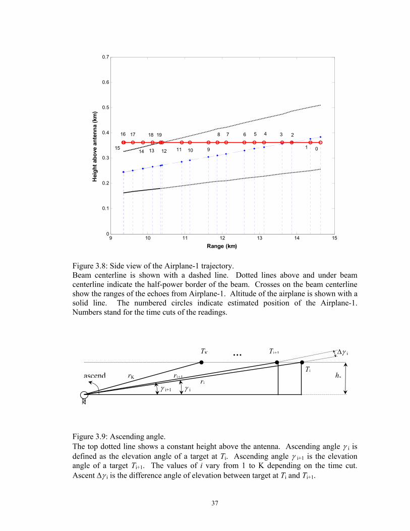
Ascending angle γ i is defined as the elevation angle of a target at Ti. The distance

between two consecutive positions of Airplane-1 can be found in terms of degrees of

ascent ∆γ i of the ascending angle γ i, as shown in Figure 3.9. The ascent ∆γ i can be

found by subtracting the ascending angle γ i created by a target at Ti from the ascending

angle γ i+1 created by a target at Ti+1

∆γ i = [sin-1(ha /r i) – sin-1(ha /r i+1)]180/π. (3.3.12)

The calculated ascending reading angles are given in Table 3.4. Negative values mean

that target Airplane-1 has turned and the angle descends.

Table 3.4: Ascending angles of Airplane-1

Between Time cuts

Angle, degrees

Between time cuts

Angle, degrees

Between time cuts

Angle, degrees

0-1 0.0267 7-8 0.0333 14-15 0.1173 1-2 0.0512 8-9 0.0362 15-16 -0.0024 2-3 0.0298 9-10 0.0804 16-17 -0.0556 3-4 0.0560 10-11 0.0377 17-18 -0.0593 4-5 0.0321 11-12 0.0955 18-19 -0.0978 5-6 0.0347 12-13 0.0514 6-7 0.0669 13-14 0.0541

36

The cross-section values spaced with the appropriate angular distances are

shown in Figure 3.10a as numbered dots. Solid lines show three Gaussian curves with

amplitudes 8, 2, and 1. The Gaussian curve corresponding to the cross-section two

square meters fits data points the best. The actual cross-section of a small craft as seen

by the radar is in the range 2 to 4 square meters [19]. The value 8 square meters is an

outlier probably caused by presence of additional scatterers in the resolution volume

(e.g. birds, other airplane), or favorable position of the aircraft.

A 5-point average of the cross-section data with dropped outlier (cut 2) is shown

in Figure 3.10b in solid line. The dashed line is used to show the fitted Gaussian curve.

The dotted line is used to show the same Gaussian curve, shifted to fit the values

corresponding to the negative ascending angles, or to the time when the airplane turned

around and started moving away from the radar. I observed several clusters of data in

Figure 3.10b, e.g. {7, 9, 11, 13}, or {8, 10, 12}. Note, that a cluster contains the data

points from either odd or even time cuts. Therefore, a possible good outcome caused by

the backlash of the antenna is ignored, e.g. {0, 3, 5, 8} make a distinct curve, but it is

ignored.

To understand the nature of these clusters, I imagined the Gaussian 2-dimension

“hat”, because the actual 3-dimension Gaussian is too hard to visualize. Any vertical

cut of the “hat”, shown in Figure 3.11, is a 1-dimension Gaussian curve. The target is

moving on through the “hat” from one curve to another, drawing spatially farther, or

closer to the top of the “hat”.

At the 13th time cut, a time when airplanes were at the same range, the cross-

section of Airplane-2 is larger than that of Airplane-1. By analyzing the flight of the

37

9 10 11 12 13 14 150

0.1

0.2

0.3

0.4

0.5

0.6

0.7

01

2345678

9101112131415

16 17 18 19

Range (km)

Hei

ght a

bove

ant

enna

(km

)

Figure 3.8: Side view of the Airplane-1 trajectory. Beam centerline is shown with a dashed line. Dotted lines above and under beam centerline indicate the half-power border of the beam. Crosses on the beam centerline show the ranges of the echoes from Airplane-1. Altitude of the airplane is shown with a solid line. The numbered circles indicate estimated position of the Airplane-1. Numbers stand for the time cuts of the readings.

Figure 3.9: Ascending angle. The top dotted line shows a constant height above the antenna. Ascending angle γ i is defined as the elevation angle of a target at Ti. Ascending angle γ i+1 is the elevation angle of a target Ti+1. The values of i vary from 1 to K depending on the time cut. Ascent ∆γ i is the difference angle of elevation between target at Ti and Ti+1.

harK

TK Ti+1

Ti ascend

riri+1

γ i+1 γ i

… ∆γ i

38

-0.5 0 0.5 1 1.50

1

2

3

4

5

6

7

8

0

1

2

3

4

5

6 7

8

9 1011 121314 15

1617 18

19

Angle (degrees)

Cro

ss-s

ectio

n (m

2 )

-0.5 0 0.5 1 1.5

0

0.5

1

1.5

2

0

1

3

4

5

6

7

8

9

10

11

12

13

14 15

1617

18

19

Angle (degrees)

Cro

ss-s

ectio

n (m

2 )

Time cutGaussianShifted Gaussian5-pt-average

Figure 3.10: Fitting Cross-section to Gaussian curve. (a) Viewing 3 curves: top curve is 8 exp(–x2/2σ b

2), middle curve is 2 exp(–x2/2σ b2),

and bottom curve is exp(–x2/2σ b2). The outlier might occur because of the presence of

other scatterers in the resolution volume (e.g. other scatterers). (b) 5-point average with dropped maximum value fits very well the Gaussian curve with amplitude 2. Note that Time cut 15 is the turning point.

39

Figure 3.11: Gaussian “hat” with fitted cross-section values. The cross-section data points are shown as black dots. Each cut of the “hat” is a 2-dimensional Gaussian.

Airplane-2, I noticed a change of its cross-section depending on the position of the

airplane. For example, the cross-section of Airplane-2 is the greatest at cuts 12, 13, and

14. During these time cuts Airplane-2 is turned sideways to the radar. As expected and

in agreement with optical cross section the EM cross section of an aircraft side is larger

then its front or back looking cross section.

3.5 Spectra

A spectrum X(ejω) of a discrete signal x[n] provides the information about the

composition of the signal from complex exponentials, and can be represented by a

linear combination of sinusoids at different frequencies

∑+∞

−∞=

−=n

njj enxeX ωω )()( . (3.5.1)

The deterministic autocorrelation rxx of a discrete signal x(n) is defined as

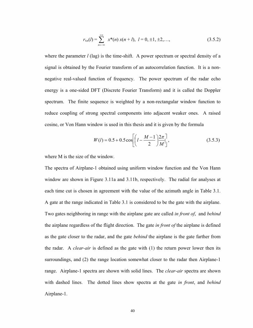
40

rxx(l) = ∑+∞

−∞=nx*(n) x(n + l), l = 0, ±1, ±2,…, (3.5.2)

where the parameter l (lag) is the time-shift. A power spectrum or spectral density of a

signal is obtained by the Fourier transform of an autocorrelation function. It is a non-

negative real-valued function of frequency. The power spectrum of the radar echo

energy is a one-sided DFT (Discrete Fourier Transform) and it is called the Doppler

spectrum. The finite sequence is weighted by a non-rectangular window function to

reduce coupling of strong spectral components into adjacent weaker ones. A raised

cosine, or Von Hann window is used in this thesis and it is given by the formula

−−+=

MMllW π2

21cos5.05.0)( , (3.5.3)

where M is the size of the window.

The spectra of Airplane-1 obtained using uniform window function and the Von Hann

window are shown in Figure 3.11a and 3.11b, respectively. The radial for analyses at

each time cut is chosen in agreement with the value of the azimuth angle in Table 3.1.

A gate at the range indicated in Table 3.1 is considered to be the gate with the airplane.

Two gates neighboring in range with the airplane gate are called in front of, and behind

the airplane regardless of the flight direction. The gate in front of the airplane is defined

as the gate closer to the radar, and the gate behind the airplane is the gate farther from

the radar. A clear-air is defined as the gate with (1) the return power lower then its

surroundings, and (2) the range location somewhat closer to the radar then Airplane-1

range. Airplane-1 spectra are shown with solid lines. The clear-air spectra are shown

with dashed lines. The dotted lines show spectra at the gate in front, and behind

Airplane-1.

41

Spectra uniformly weighted Spectra weighted with Von Hann window

-40 -20 0 20 40-80

-60

-40

-20

0

20

40

60

Velocity (ms-1)

Pow

er (d

B)

in front ofairplanebehindclear air

-40 -20 0 20 40-80

-60

-40

-20

0

20

40

60

Velocity (ms-1)

Pow

er (d

B)

a b Figure 3.11: Spectra from the Airplane-1-gate at Cut 2 (Table 3.1), the gates in front of and behind the Airplane-1-gate and spectrum of clear-air: (a) uniformly weighted spectra, (b) weighted by the Vonn Hann window. Solid line indicates spectra of the gate with Airplane-1. Dotted lines show spectra at the gates in front of and behind the Airplane-1 gate. Dashed line is for clear-air. In front of the gate spectrum shows clear-air. Behind the gate spectrum repeats the airplane spectrum with smaller amplitude, due to the spread of the range dependant weighting function. Spectra shows 10 well pronounced peaks due to modulation caused by propeller rotation.

For each time cut figures similar to Figures 3.11a and 3.11b were generated and

analyzed. For some cuts the spectrum at the gates in front of and behind the airplane

gate shows similar shape to the airplane gate but with smaller amplitude. This is due to

the spread of the skirt of the range-dependent part of the composite weighting function.

The clear-air spectra in all 20 cuts show similar Gaussian-shape curve centered

between –3 and –5 ms-1. As noted in Section 2.5.2, the wind was blowing from south –

42

south-east at about 5 ms-1. The peak corresponding to velocity 24 ms-1 indicates that

Airplane-1 is moving at either 24 ms–1 away from the radar or 40 ms–1 toward radar, as

described in Section 3.2.2. The clear-air spectrum is 40dB below the airplane

spectrum. Another interesting common feature in the Airplane-1 spectrum is 10 well

pronounced peaks, with one maximum. All 20 spectra have similar signature with a

slight variation of amplitudes and fluctuations of the location of maxima. The peaks are

spaced by 6 to 7 ms-1 interval. The 10 peaks could help to distinguish these spectra

from other types of scatterers.

For comparison, similar analyses are done for Airplane-2. All eleven spectra of

Airplane-2 echoes are similar to the one shown in Figures 3.12a. The solid line

indicates the spectrum from the airplane gate. The dotted lines indicate spectrum from

the gates in front of and behind Airplane-2. The dashed line is the spectrum of the

clear-air. There are several similarities in the Airplane-1 and the Airplane-2 spectra. A

range dependant repetition of the spectrum is observed in both cases. The radial

component of the wind speed is the same for both cases. The maximum in the airplane

spectra corresponds to the radial velocity of Airplane-2, similar to what was observed in

Airplane-1 case. Unlike Airplane-1, the spectra of Airplane-2 do not exhibit

modulations. It could be that Airplane-2 propellers are small compared to the

dimensions of the airplane, or it is a jet airplane. The spectra from neighboring gates

repeat the airplane spectrum with smaller amplitude, due to the spread of the range

dependant weighting function. The peak at zero velocity in the clear-air spectra is due

to the ground clutter. Animating spectra time allows observing fluctuations and

distinguishing between little changes in the airplane spectra from the unique features

43

that are approximately constant. The extracted features would define the airplane

signature. Thus, the types of airplanes may be distinguished by their spectra, if they

indeed have the unique signatures.

Spectra uniformly weighted Spectra weighted with Von Hann window

-40 -20 0 20 40-60

-40

-20

0

20

40

60

Velocity (ms-1)

Pow

er (d

B)

in front ofairplanebehindclear air

-40 -20 0 20 40-40

-30

-20

-10

0

10

20

30

40

50

Velocity (ms-1)

Pow

er (d

B)

a b Figure 3.12: Spectra from the Airplane-2-gate at Cut 10 (Table 3.2), the gates in front of and behind the Airplane-1-gate and spectrum of clear-air: (a) uniformly weighted spectra, (b) weighted by the Vonn Hann window. Solid line indicates spectra of the gate with Airplane-2. Dotted line shows spectra at the gates in front and behind the Airplane-1 gate. Dashed line is for Clear-air. The spectra from neighboring gates repeat the airplane spectrum with smaller amplitude, due to the spread of the range dependant weighting function

3.6 Modulations

In Section 3.4 modulation is apparent in spectra of Airplane-1. It is

hypothesized that these modulations are likely caused by propeller rotation. In each

spectrum there are 10 almost equally spaced maxima. The spacing between two

consecutive peaks is approximately between 6 and 7 ms-1.

44

In the Homeland Security Experiment document CR1 Test Plan of 19 Mar 2003,

it is stated that the aircraft used in the experiment is a Cessna 188 AgWagon, shown in

Figure 3.13. Such airplanes have 235 to 300 horsepower and 2-bladed propellers. In

this section simulations are used to demonstrate that similar modulation can be

produced. Airplane-2 is an unknown aircraft, and the discussion on it is closed due to

uncertainty of all the discoveries and inability to prove or contradict the results.

Figure 3.13: Cessna 188 Ag Wagon. The propeller has 2 blades.

If a propeller is spinning at 2400 rpm or 40 revolutions per second, then any

blade of the propeller passes a specific point in the arc 40 times every second. It would

take 0.025 seconds for a blade to make one revolution. The signal from a flying

airplane with a propeller is affected by many factors: (1) the speed of flight and the

position of the airplane in the volume of scan, (2) the propeller rotation speed, (3) the

weather factors affecting flight (shaking due to winds, shear), and (4) moving of the

airplane parts, as ailerons (movable outside edges of the wing, that turn the plane),

flaps (part of the wing that can move down to act as brakes), and elevator (tail part of

the plane that moves to make the plane pitch up or down). In this work, only a simple

model is used, shown in Figure 3.14. In other words, the weather and the moving parts

except the propeller could be neglected.

45

Figure 3.14: Simple model for detection of a signal modulated by a 2-bladed propeller. Radar beam radiates toward the airplane (bold velocity vector) moving forward, and the rotating propeller (black curved arrows).

A received signal y(k) produced by an airplane with a constant speed, and a

rotating propeller can be written in the form

( ) ( ) ( ))(exp)(expexp)( 11 ωωωωω ++−+= ddd jkBjkBjkAky , (3.7.1)

where A is amplitude caused by the airplane’s main body, B is amplitude of a signal

reflected from the propeller, ω d is the Doppler shift due to the airplane movement, ω 1 is

the shift caused by propeller blade (moving toward or away from the radar, curved

arrows in Figure 3.14). The propeller causes reflections which in turn create

modulations if the airplane is not flying along beam axis. Even if the plane is aligned

on the average with the beam axis, instantaneous deviations due to pitch and yaw will

be present. The Doppler shift from the propeller depends on the location of dominant

scatterers. If the scatterers are equally strong along the propeller then the shift will have

a distribution between 0 (corresponding to propeller center) and the maximum value at

the end of propeller blade. The simplified model herein assumes dominant scatterers

are confined at some distance from the center hence the modulation can be represented

with a single sinusoid ω1 = C sin(α t)t = kT , with an amplitude C, and α = 2π (rpm/60 ×

blades), where rpm is the propeller speed in revolutions per minute, blades is the

number of the blades on the propeller, and sampling rate T = 7.8×10-4. White noise is

added to the signal. The modeled signal is sampled at the radar PRF, and the DFT of

Radar beam

46

the result is taken. Spectral signatures are investigated using several propeller speeds

from 1000 up to 5000 rpm, different airplane speeds from 40 to 55 ms-1, and different

amplitude values A, B, C. It was found that observed spectra can be reproduced in

simulation when a speed of 41 ms-1, a 2-bladed propeller rotating at 2400 rpm were

used. The resulting signal and its spectrum are shown in Figures 3.14a and 3.15

respectively.

0 0.005 0.01 0.015 0.02 0.025 0.03 0.035 0.04 0.045 0.05-10

-5

0

5

10

Time (s) a

0 0.005 0.01 0.015 0.02 0.025 0.03 0.035 0.04 0.045 0.05-10

-5

0

5

10

Time (s)

b Figure 3.14: I-Q samples of (a) the actual signal from airplane registered during 5th time cut in the 54th range location of radial 171.9°, (b) simulated signal, obtained from the sampling at radar PRF of a continuous signal, modeled by a craft moving at 41m/s with a 2-bladed propeller rotating at 2400 rpm. The amplitudes of the simulated airplane body and propeller returns are 2 and 0.5 respectively (A=2, B=.5, C=248).

Simulation result has demonstrated that an airplane echo contains the signature

of propeller rotation. A more complicated model of an airplane would include (1) a

--- Q I

--- Q I

47

function of the airplane cross-section change due to tilt and turn, and (2) a function of

airplane speed variation.

Spectra uniformly weighted Spectra weighted with Von Hann window

-40 -20 0 20 405

10

15

20

25

30

35

40

45

50

Velocity (ms-1)

Pow

er (d

B)

-40 -20 0 20 400

5

10

15

20

25

30

35

40

45

Velocity (ms-1)

Pow

er (d

B)

a b

Figure 3.15: Spectra of the simulated signal from a craft moving at 41ms-1 with a 2-bladed propeller rotating at 2400rpm: (a) uniformly weighted; (b) weighted by the Von Hann window.

3.7 Conclusion

An airplane has features in its spectra corresponding to the physical

specifications of the craft. Airplanes could be distinguished by their spectra. The

simple model of the airplane replicated spectral characteristics of Cessna 188 Ag

Wagon.

48

4. Birds

The goal of this section is to investigate spectra of birds. These bird spectrum

signatures could be used in distinguishing these echoes for filtering the weather signals,

or obtaining information for ornithological studies.

4.1 Single Birds from data set 3/26

The same data as used in Chapter 3 include bird echoes. The velocity and

reflectivity PPIs shown in Figures 3.2a and 3.2b contain a number of specks with

nonzero velocities (not related to the wind speed) corresponding to small reflectivity

values. These specks might be birds. An example of the returned power along the

178.6° radial is shown in Figure 4.1a for all 468 range locations and in Figure 4.1b for

only 85 range locations to magnify features.

The pointers in Figure 4.1b indicate ground clutter and birds. It is not possible

to distinguish the nature of the return looking at the returned power peaks. The decision

on the nature of the scatterers can be made either by (1) spectral analysis/velocity

estimation or by (2) visual analysis of the real part of voltage. The evidence of ground

clutter in Doppler spectra is a peak at zero velocity. The evidence of ground clutter in

the time domain is a slowly varying, almost DC signal. The I components of the

received I-Q samples (Figure 4.2), corresponding to some of the peaks in Figure 4.1b,

demonstrate significant visual differences that may be used to classify observed peaks

on ground clutter returns and returns from birds. Figure 4.2a shows sinusoid signals

that are most likely returned from birds. Figures 4.2b and 4.2c demonstrate ground

clutter signals and contaminated signal from both birds and ground clutter, respectively.

There are 3 strong presumable bird returns in the observed radial presented in Figure

49

4.1b: (1) an echo from range 6.2 km (gate 28), (2) an echo from 7.6 km (gate 34), and

(3) an echo from 11.5 km (gate 49). I assume these returns are birds, though they might

be the sidelobe returns from vehicles on the ground. The spectra of these gates

weighted with the Von Hann window are displayed in Figure 4.3.

50 100 150 200 250 300 350 400 450-40

-20

0

20

40

Range gates

Pow

er, d

B

0 10 20 30 40 50 60 70 80-40

-20

0

20

40

60

Range gates

Pow

er, d

B

cut 3 radial 178.6o

cut 3 radial 178.6o

Figure 4.1: The return power of the radial 178.6° at time cut 3. Top: All 468 range locations. Bottom: 85 range locations. Only close ranges considered. The ground clutter returns are indicated by solid circles. The bird(s) returns are indicated by clear circles. The bird contaminated by ground clutter returns are indicated by arrows.

Evaluating spectra and voltages, I have chosen a bird that is closest to the radar

and called it Bird-1. To investigate the behavior of the signal depending on the

direction of the bird’s flight, I have chosen another bird from a different radial and

50

0 10 20 30 40 50 60 70-0.4

-0.2

0

0.2

0.4

0 10 20 30 40 50 60 70-0.2

0

0.2

0.4

0.6

0 10 20 30 40 50 60 700

0.05

0.1

gate 28gate 34gate 49

gate 20gate 23gate 36

gate 24gate 37

Figure 4.2: The real part of return voltage of the radial at 178.6° from: (top) birds, (middle) ground clutter; (bottom) bird contaminated by the ground clutter. Gate 28: DFT with Von Hann Gate 34: DFT with Von Hann Gate 49: DFT with Von Hann

-20 0 20-60

-50

-40

-30

-20

-10

0

10

20

Velocity (ms-1)

Pow

er (d

B)

-20 0 20-60

-50

-40

-30

-20

-10

0

10

20

Velocity (ms-1)

Pow

er (d

B)

-20 0 20-60

-50

-40

-30

-20

-10

0

10

20

Velocity (ms-1)

Pow

er (d

B)

Figure 4.3: Spectra of birds in radial 178.6° at time cut 3. All shown spectra are weighted with the Von Hann window. The solid line indicates the spectrum at the gate with the bird. The dotted and dashed lines show the spectra in front of, and behind the gate with the bird respectively.

Pulse Number

Pulse Number

Pulse Number

Birds

____ gate 24 __ __ gate 37

51

called it Bird-2. Bird-2 was moving in the direction somewhat opposite to that of

Bird-1. Bird-2 was flying against the radial velocity component of the wind, while

Bird-1 was flying with the radial velocity components of the wind.

4.1.1 Tracking

Tracking of birds was similar to airplane tracking described in Section 3.1

because at close ranges (5 to 8 km) the reflectivity of bird echoes is relatively strong

(about 15 dBZ) and easily seen on the reflectivity display of RRAT. The trajectories of

Bird-1 and Bird-2 are shown in Figure 4.4. The Bird-1 track is almost straight, but the

Bird-2 trajectory is complex. During the 7th time cut Bird-2 is being carried by the

wind. The reflectivity, azimuth and range values of Bird-1 and Bird-2 are given in

Table 4.1 and Table 4.2 respectively. The spectra of Bird-1 and Bird-2 for several time

cuts are shown in Figures 4.5 and 4.6 respectively. It is interesting to note that all 20

(one for each cut) Bird-1 spectra look very similar, each having a single prominent

maximum. However Bird-2 spectra vary. Bird-2 is flying straight only during time cuts

0 through 6. During the time of the 7th through 19th time cuts, the spectra of Bird-2

changes could be due to diving, circling, and accelerating of the bird, and contamination

by other birds, as described in Section 4.2. The overall speeds of flight estimated from

bird trajectories are 10.3 ms-1 for Bird-1 and 6.9 ms-1 for Bird-2, a little bit larger than

the radial velocities estimated from spectra 9 ms-1 for Bird-1 and 6 ms-1 for Bird-2. As

expected, the bird flying against the radial velocity of the wind goes slower.

4.1.2 Cross section

The cross sections of the birds were calculated according to equation (3.3.9).

The cross section values of Bird-1 are about 1000 times smaller than those of the airplanes,

52

Fig 4.4: The trajectories of Bird-1 and Bird-2. The direction of the wind is indicated. A 1° azimuth angle corresponds to 133 m at a range 8 km, and to 83 m at a range 5 km.

and fluctuate from 0.1×10–4 to 5.7×10–4 m2. The variation (factor of 57) could be due to

the bird orientation and its location in the resolution volume. The cross section value of

Bird-2 exhibit similar behavior up to the 10th time cut; however, the variations in cross

18 19 14, 15 17

16 13 10 12 11 9 7 8 5 4 6 3 1 2 0

180 170 190Azimuth (degree)

Range (km)

185

6 Wind

1 0 3 8 5 2 4 11 9 7 6 12 10 15 17 14 19 13 18 16

Bird-2

Bird-1

175

490 m

580 m

665 m

7

5

410 m

53

section for later cuts are considerable. Large cross section values for time cuts 15, 16

and 17 imply presence of ground clutter or other birds in the resolution volume. The

spectra for these time cuts are described in Section 4.2.

The spectrum of a single flying bird that is free from other scatterers consists of

a narrow large maximum centered at the bird’s radial velocity. Figure 4.7 displays such

spectra for Bird-1 in the top two plots and for Bird-2 in the bottom two plots. The

spectra to the left are from uniformly weighted time-series and the spectra to the right

are obtained with the Von Hann windows. The solid line shows the spectrum at the

gate with the bird. The dotted lines show spectra in neighboring gates. Maximum

values in each plot correspond to the radial velocity of the bird.

The contribution due to the wing beating is not possible to distinguish. The

double peak of Bird-2 (Figure 4.7 bottom left) is probably an indication of the presence

of another bird in the resolution volume with a slightly larger radial velocity.

It is possible to identify the wind velocity from the uniformly weighted spectra

for Bird-1, though it is not obvious. The spectra weighted with the Von Hann window

demonstrates a well defined peak at –4 ms–1 with power –12 dB at the Bird-1 location

and with power up to –5 dB at a neighboring to the Bird-1 range location. This peak is

the wind velocity (Section 2.5.2). The wind velocity peak is easy to observe in both

Bird-2 spectra.

Ground Clutter returns in Figure 4.7 are centered at zero velocity values and are

small (in this particular radial) in comparison to the bird returns.

54

Table 4.1: Reflectivity and cross-section of Bird-1

Cut Time

t

(h:m:s)

Target Range

r (km)

AzimuthAngle θ

(°)

Radial Velocity

v (m/s)

Reflec-tivity

Z (dBZ)

Equivalent Reflectivity

Factor Ze

(mm6m–3)

Reflectivity Per Unit Volume η×109

(mm6m–3m-4)

Cross- section σb

(m2) 0 10:29:21 6.63 178.2 12 4 3 0.007 0.1×10-4

1 10:29:33 6.38 179.3 13 6 4 0.011 0.2×10-4

2 10:29:39 6.38 177.8 12 16 40 0.113 1.7×10-4

3 10:29:48 6.13 178.6 12 16 40 0.113 1.6×10-4

4 10:29:56 5.88 177.1 16 18 63 0.180 2.3×10-4

5 10:30:03 5.88 177.7 12 22 159 0.451 5.7×10-4

6 10:30:10 5.88 176.2 16 20 100 0.285 3.6×10-4

7 10:30:19 5.63 176.3 8 20 100 0.285 3.3×10-4

8 10:30:26 5.63 175.0 12 18 63 0.180 2.1×10-4

9 10:30:34 5.63 175.6 12 18 63 0.180 2.1×10-4

10 10:30:42 5.38 174.9 12 14 25 0.072 0.8×10-4

11 10:30:50 5.38 174.6 12 16 40 0.113 1.2×10-4

12 10:30:57 5.38 172.8 10 14 25 0.072 0.8×10-4

13 10:31:05 5.38 173.3 8 14 25 0.072 0.8×10-4

14 10:31:12 5.13 171.5 0 22 159 0.451 4.4×10-4

15 10:31:21 5.13 171.5 12 20 100 0.285 2.8×10-4

16 10:31:28 5.13 170.3 10 20 100 0.285 2.8×10-4

17 10:31:36 5.13 170.0 0 20 100 0.285 2.8×10-4

18 10:31:43 4.88 168.7 10 20 100 0.285 2.5×10-4

19 10:31:50 4.88 168.7 8 22 159 0.451 3.9×10-4

-20 0 20-60

-50

-40

-30

-20

-10

0

10

20

FFT*VonHann

Velocity (ms-1)

Pow

er (d

B)

-20 0 20-60

-50

-40

-30

-20

-10

0

10

20

FFT*VonHann

Velocity (ms-1)-20 0 20

-60

-50

-40

-30

-20

-10

0

10

20

FFT*VonHann

Velocity (ms-1)-20 0 20

-60

-50

-40

-30

-20

-10

0

10

20

FFT*VonHann

Velocity (ms-1)

Cut 1 Cut 2 Cut 3 Cut 4 Figure 4.5: Bird-1 spectra. The locations of echoes for indicated cuts are given in Table 4.1. The solid line shows spectrum at the gate with Bird-1. The dotted and dashed lines show spectra from the neighboring gates. All spectra are weighted with the Von Hann window.

Bird-1

55

Table 4.2: Reflectivity and cross-section of Bird-2

Cut

Time t

(h:m:s)

Target Range

r (km)

AzimuthAngle θ

(°)

Radial Velocty

v (m/s)

Reflec-tivity

Z (dBZ)

Equivalent Reflectivity

Factor Ze

(mm6m–3)

Reflectivity Per Unit Volume η×109

(mm6m–3m-4)

Cross- section σb

(m2) 0 10:29:21 7.1 178.0 +14 10 10.00 0.03 1×10-4

1 10:29:33 7.1 179.2 +10 19 79.43 0.23 4×10-4

2 10:29:39 7.2 179.4 +12 12 15.85 0.05 1×10-4

3 10:29:48 7.2 180.8 +7 19 79.43 0.23 4×10-4

4 10:29:56 7.3 180.7 +10 7 5.01 0.01 2×10-4

5 10:30:03 7.3 182.1 +12 16 39.81 0.11 1×10-4

6 10:30:10 7.5 182.0 +6 11 12.59 0.04 1×10-4

7 10:30:19 7.5 183.0 +7 13 19.95 0.06 1×10-4

8 10:30:26 7.3 184.5 +14 22 158.49 0.45 9×10-4

9 10:30:34 7.5 185.6 +14 21 125.89 0.36 7×10-4

10 10:30:42 7.7 185.3 +16 25 316.23 0.90 20×10-4

11 10:30:50 7.5 186.1 +16 21 125.89 0.36 7×10-4

12 10:30:57 7.7 185.8 +10 21 125.89 0.36 8×10-4

13 10:31:05 8.0 186.6 +10 21 125.89 0.36 8×10-4

14 10:31:12 7.9 185.8 +5 23 199.53 0.57 13×10-4

15 10:31:21 7.9 186.9 +8 30 1000.00 2.85 65×10-4

16 10:31:28 8.1 186.7 +8 34 2511.89 7.15 172×10-4

17 10:31:36 7.9 187.4 +8 34 2511.89 7.15 163×10-4

18 10:31:43 8.0 187.0 -13 30 1000.00 2.85 66×10-4

19 10:31:50 8.0 187.8 -16 30 1000.00 2.85 66×10-4

-20 0 20-60

-50

-40

-30

-20

-10

0

10

20

FFT*VonHann

Velocity (ms-1)

Pow

er (d

B)

-20 0 20-60

-50

-40

-30

-20

-10

0

10

20

FFT*VonHann

Velocity (ms-1)-20 0 20

-60

-50

-40

-30

-20

-10

0

10

20

FFT*VonHann

Velocity (ms-1)-20 0 20

-60

-50

-40

-30

-20

-10

0

10

20

FFT*VonHann

Velocity (ms-1) Cut 1 Cut 2 Cut 3 Cut 4 Figure 4.6: Bird-2 spectra. The locations of echoes for indicated cuts are given in Table 4.2. The solid line shows spectrum from the gate with Bird-2. The dotted and dashed lines show spectra from the neighboring gates. All spectra are weighted with the Von Hann window.

Bird-2

56

Bird-1: Spectra uniformly weighted Bird-1: Spectra weighted with Von Hann Window

-20 0 20-60

-50

-40

-30

-20

-10

0

10

20

Velocity (ms-1)

Pow

er (d

B)

-20 0 20-60

-50

-40

-30

-20

-10

0

10

20

Velocity (ms-1)

Pow

er (d

B)

Bird-2: Spectra uniformly weighted Bird-2: Spectra weighted with Von Hann Window

-20 0 20-60

-50

-40

-30

-20

-10

0

10

20

Velocity (ms-1)

Pow

er (d

B)

-20 0 20-60

-50

-40

-30

-20

-10

0

10

20

Velocity (ms-1)

Pow

er (d

B)

Figure 4.7: Single bird spectra. Spectra to the right are weighted with the Von Hann window. The solid line shows the spectra from the gate with the bird. The dotted lines show spectra from neighboring gates. Maximum in each plot corresponds to the radial velocity of the bird.

Wind Wind

Bird Bird

Wind Wind

Bird Bird

57

4.1.3 Simulation

A simple model of a flying bird is shown in Figure 4.8.

Figure 4.8: Simple model for detection of a signal scattered by a bird. The radar beam hits the bird (bold black arrow) moving forward, and the wings moving up or down (black curved arrows) as indicated.

The underlying assumption is that the bird’s cross section periodically changes

with a position of the wings. Therefore the amplitude of the return can be approximated

with a constant part due to the bird’s body and a modulating part caused by the wings,

as expressed in the following equation

kkBAjkkBAky dd ωωωω sin)sin(cos)sin()( 11 +++= . (4.7.1)

A is the amplitude of a flying bird, B is the amplitude of a signal modulated by a wing

beat, ωd is the Doppler shift due to the bird movement, and ω1 is the shift caused by

wings moving up and down. Wings are thought to flap simultaneously, and therefore

the shift is modeled as a sinusoid ω1 = C sin(2πFbeatt)t = kT, where Fbeat is the frequency

of the beating wings, C is the amplitude, and T = 7.8×10-4. White noise is added to the

signal (SNR ~30 dB). The modeled signal is sampled, and the discrete Fourier

Transform (DFT) of the result is taken.

The variables in the simulation are wing beat frequency, and the values of

amplitudes A, B, C. The shape of the spectrum for a signal without noise changes as

follows. Define an extra peak on the slope of the peak corresponding to the radial

velocity of a bird as a wing-beat-spike. A signal modulated by wing beating

Radar beam

58

demonstrates appearance of wing-beat-spikes on the slopes of the spectral peak for

frequencies more then 8 Hz (Figure 4.9a, and 4.9b). Unfortunately large birds wings

beating frequencies are less then 2 Hz which cannot be distinguished from the obtained

spectra (Figure 4.9c and 4.9d).

Spectra uniformly weighted Spectra uniformly weighted

a b

Spectra uniformly weighted Spectra uniformly weighted

c d

Figure 4.9: Wing beating simulation without noise. Velocity of the simulated bird 7ms–1, wing beating frequency: (a) 12 Hz, (b) 8Hz, (c) 2 Hz, (d) 1Hz. An extra peak on the slope of the peak corresponding to the radial velocity of a bird is defined as a wing-beat-spike. The wing-beat-spikes are observed only at wing beating frequencies less then 2 Hz.

59

A bird signal was simulated with different radial velocities, wing beating

frequencies (Figure 4.10 top), amplitudes of the bird body (Figure 4.10 bottom), and

amplitudes of the wings.

Spectra uniformly weighted Spectra weighted with Von Hann Window

-20 0 20-60

-50

-40

-30

-20

-10

0

10

20

Velocity (ms-1)

Pow

er (d

B)

-20 0 20-60

-50

-40

-30

-20

-10

0

10

20

Velocity (ms-1)

Pow

er (d

B)

Spectra uniformly weighted Spectra weighted with Von Hann Window

-20 0 20-60

-50

-40

-30

-20

-10

0

10

20

Velocity (ms-1)

Pow

er (d

B)

-20 0 20-60

-50

-40

-30

-20

-10

0

10

20

Velocity (ms-1)

Pow

er (d

B)

Figure 4.10: Example of variables for Bird-1 simulation with noise. Velocity of the simulated bird is 9 ms–1. Top: Wing beating frequencies are in the range from 0.1 Hz to 8 Hz; Bottom: Amplitudes of the bird body are from 0.1 to 0.5. The spectra to the left are uniformly weighted, while the spectra to the right are weighted with the Von Hann window.

60

The wing beating frequency cannot be observed in presented spectra. The

strength of the radial velocity peak in spectra depends on the bird’s body amplitude.

Larger bird shows stronger signal with the same SNR. The best matches of the modeled

spectra for Bird-1 and Bird-2 are shown in Figure 4.11a and 4.11b, respectively.

Spectra uniformly weighted Spectra weighted with Von Hann Window

-20 0 20-60

-50

-40

-30

-20

-10

0

10

20

Velocity (ms-1)

Pow

er (d

B)

-20 0 20-60

-50

-40

-30

-20

-10

0

10

20

Velocity (ms-1)

Pow

er (d

B)

Spectra uniformly weighted Spectra weighted with Von Hann Window

-20 0 20-60

-50

-40

-30

-20

-10

0

10

20

Velocity (ms-1)

Pow

er (d

B)

-20 0 20-60

-50

-40

-30

-20

-10

0

10

20

Velocity (ms-1)

Pow

er (d

B)

Figure 4.11: Birds simulation. Top: Bird-1 spectra: radial velocity 9.6 ms–1 (A=0.4, B=0.1, C=1). Bottom: Bird-2 spectra: radial velocity 6.9 ms–1 (A=0.1, B=0.3, C=1). The spectra to the left are uniformly weighted, while the spectra to the right are weighted with the Von Hann window.

61

The modeled Bird-1 and Bird-2 radial velocities are 9.6 ms–1 and 6.9 ms–1,

respectively. The amplitudes for Bird-1 are A=0.4, B=0.1, C=1, when those for Bird-2

are A=0.1, B=0.3, C=1. Bird-1 is simulated to have big body and small wings (ratio

4/1), when Bird-2 has a small body and large wings (ratio 1/3). But overall, Bird-1 is

supposed to be a little larger then Bird-2 (ratio 4/3) and this can be seen from the

spectra.

Clear-air wind can be included in the simulation as shown in Figure 4.12. The

spectrum of Bird-1, shown in Figure 4.7 in the top plots is matched with the spectrum of

the modeled signal with additive wind 4 ms–1, bird radial velocity 7 ms–1.

Spectra uniformly weighted Spectra weighted with the Von Hann window

-20 0 20-60

-50

-40

-30

-20

-10

0

10

20

Velocity (ms-1)

Pow

er (d

B)

-20 0 20-60

-50

-40

-30

-20

-10

0

10

20

Velocity (ms-1)

Pow

er (d

B)

a b

Figure 4.12: Bird-1 with the wind simulation. (a) Spectrum of Bird-1 uniformly weighted. (b) Spectrum of Bird-1 weighted with the Von Hann window. Solid line indicates simulated spectrum. Dotted line shows actual spectrum. Note presence of the ground clutter (GC) in the actual spectrum. Bird- and wind- radial velocities are indicated.

Wind

Bird

Wind

Bird

Simulation Actual Spectra

GC

62

4.2 Multiple Birds from data set 3/26

Several spectra of multiple birds taken at the locations with registered Bird-2

echo are shown in Figure 4.13. All spectra are weighted with the Von Hann window.

Spectra weighted with the Von Hann window Spectra weighted with the Von Hann window

-40 -20 0 20 40-80

-70

-60

-50

-40

-30

-20

-10

0

10

Velocity (ms-1)

Pow

er (d

B)

-40 -20 0 20 40-60

-50

-40

-30

-20

-10

0

10

20

30

Velocity (ms-1)

Pow

er (d

B)

9th time cut 16th time cut Figure 4.13: Multiple birds’ spectra. All spectra are weighted with the Von Hann window. The solid line shows the spectra at the gate with the registered bird. The dotted lines show spectra in neighboring gates. The dashed line shows clear-air spectrum. Local maxima in each plot correspond to the radial velocity of birds. The local maxima corresponding to zero velocity are assumed due to ground clutter.

Other local maxima correspond to the radial velocity of the birds. Obviously, one of the

maxima (indicated by arrow) is contributed by Bird-2 tracked in Section 4.1. The solid

lines in the spectra for the 9th and the 16th time cuts and their neighbors show several

birds flying in different directions, and ground clutter. Due to the spread of the range

dependant weighting function, the spectrum at a gate is affected by the signals in the

Bird-2

63

neighboring gates. In other words, a point scatterer is detectable in its neighboring

resolution volumes. This phenomenon causes the spectra for the 16th time cut in Figure

4.13 to show a repetition (in neighboring gates) of peaks for Bird-2 flying at about 15

ms–1 toward radar, and a repetition of peaks for another bird moving at about 10 ms

away from the radar. There is another peak in this spectra corresponding to the radial

velocity about 5 ms–1 away from the radar. This one does not display repetition in

neighboring gates probably because it is on the edge of the neighborhood of the

detectable cluster.

4.3 Multiple Birds from data set 5/8

Data 5/8 was collected after a tornadic super-cell. The PPI of RRAT (Figure

4.14a and 4.14b) shows small reflectivity values ranging from -5dBZ to +15dBZ at

ranges up to 40 km, and velocities with values from -32 ms–1 to +32 ms–1. A part of PPI

is magnified to display features (Figure 4.14c and 4.14d). The sounding (Table 4.3)

shows that the wind speed was varying from 32 knots to 35 knots (16.5 – 18 ms–1), and

then calmed down to 24 knots. Radar meteorologists claimed that these echoes are

from biological scatterers and the wind from South.

Table 4.3: Sounding 72357 OUN Norman Observations at

Time & Date

Height, m

Direction, degree

Speed, Knot

Reference http://weather.uwyo.edu/cgi-bin/

sounding?region=naconf&TYPE=TEXT%3ALIST&

12Z 5/8

2003

610 686 914

170 170 180

34 32 35

YEAR=2003&MONTH=05& FROM=0812&TO=0900&

STNM=72357

00Z 5/9

2003

610 719 814 914

210 215 222 230

24 22 21 19

YEAR=2003&MONTH=05& FROM=0900&TO=0912&

STNM=72357

64

a b

c d Figure 4.14: Cut 3, elevation 2.5°, PRT 986 µs. (a) Reflectivity PPI. (b) Velocity PPI. Areas between 5 and 10 km south from the radar as indicated by squares in (a) and (b) are magnified in (c) and (d). Range rings are 5 km apart.

Radial 176° and its neighbors 175.5° and 176.5° are chosen arbitrarily to explore

the echo features. Echo power along the chosen radials is shown in Figure 4.15. The

beam’s elevation is 2.5°; therefore, only close ranges (5-10 km, corresponding to 20th

55 kkmm

1100 kkmm

55 kkmm

1100 kkmm

55 kkmm

1100 kkmm

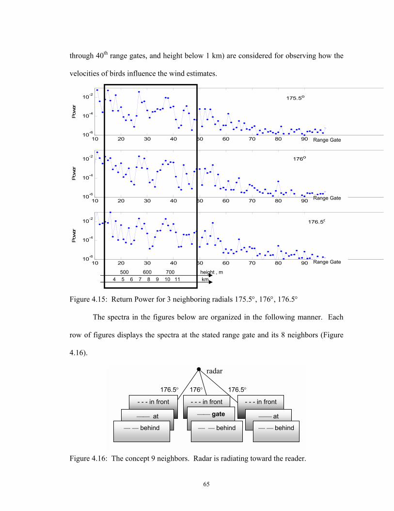
65

through 40th range gates, and height below 1 km) are considered for observing how the

velocities of birds influence the wind estimates.

10 20 30 40 50 60 70 80 9010-6

10-4

10-2

Pow

er

10 20 30 40 50 60 70 80 9010-6

10-4

10-2

Pow

er

10 20 30 40 50 60 70 80 9010-6

10-4

10-2

Pow

er

175.5o

176o

176.5o

Figure 4.15: Return Power for 3 neighboring radials 175.5°, 176°, 176.5°

The spectra in the figures below are organized in the following manner. Each

row of figures displays the spectra at the stated range gate and its 8 neighbors (Figure

4.16).

Figure 4.16: The concept 9 neighbors. Radar is radiating toward the reader.

- - - in front

at

behind

- - - in front

gate

behind

- - - in front

at

behind

radar

176.5° 176° 176.5°

4 5 6 7 8 9 10 11 km 500 600 700 height , m

Range Gate

Range Gate

Range Gate

66

The spectra of the gates evaluated in Table 4.4 are estimated.

Table 4.4: The target solutions for several gates of the chosen radials RRAT Z, dB RRAT Velocity,

ms–1

Range gate

Range,

km

Height,

M 175.5°

176°

176.5°

175.5°

176°

176.5°

Ground Clutter observation in spectra, Z, dB

15 3.5 450 4 10 7 Above 1016 3.75 460 4 10 7 -13 -16 -12 Above 1018 4 490 5 5 6 -12 -14 -15 Below 022 5 510 8 8 12 -21 -18 -14 Below 023 5.5 530 1 3 1 -14 -18 -17 Below 027 6.25 570 9 16 9 -27 -27 -27 Below-1029 6.75 590 8 10 11 28 -24 -27 None32 7.5 620 11 5 14 -26 -20 -20 Below -2034 8 650 12 17 19 -18 -27 -26 Below-2036 8.75 670 26 22 25 27 27 27 Below -537 9 690 25 21 20 -28 28 27 Below-539 9.25 710 17 20 21 -23 -25 -27 None40 9.5 720 12 9 11 -19 -21 -27 None44 10.5 760 5 3 10 -20 -20 -26 Below -1545 10.75 770 3 4 16 -20 -20 22 Below -2048 11.5 810 8 16 20 -24 27 27 Below -20

All spectra demonstrate broad multiple peaks of low power. Each spectrum

shows a peak at a velocity of approximately -20 ms–1. Slow small change in spectral

peak intensity between -10 and -15 dBZ and gradual change in velocity of the peak

from -16 ms–1 to -20 ms–1 convinced me to assume that the peak is caused by the wind.

The assumed wind velocity values are smaller than those in Table 4.4. The zero-

velocity peak that was observed in many spectra corresponds to ground clutter and is

visible in all 9 neighbors. The other peaks are due to birds, e.g. gate 15 (–22 ms–1), gate

16 (–22 ms–1), gate 18 (–22ms–1, -25 ms–1), gate 29 (–26 ms–1), gate 32 (–10 ms–1), gate

34 (+22 ms–1, –10 ms–1), and so on. The velocities of birds are larger than those of the

wind and cause higher estimates in Table 4.4 and on the velocity displays. The spectra

of the gate 27th 9-neighbohood (Figure 4.17) show that the wind velocity is

67

distinguishable from the bird velocities. For resolving data contaminated by migrating

bird velocity it is necessary to inspect the spectra for 2 (or more) peaks.

-20 0 20-40

-35

-30

-25

-20

-15

-10

-5

0

5

10

15DFT: Gate 27, Radial 175.5

Velocity (ms-1)

Pow

er (d

B)

-20 0 20-40

-35

-30

-25

-20

-15

-10

-5

0

5

10

15Radial 176

Velocity (ms-1)

Pow

er (d

B)

-20 0 20-40

-35

-30

-25

-20

-15

-10

-5

0

5

10

15Radial 176.5

Velocity (ms-1)

Pow

er (d

B)

in frontatbehind

in frontatbehind

in frontatbehind

Figure 4.17: Distinguishing between wind and birds velocities. Solid bold line indicates the wind velocity. Birds are shown with arrows. All spectra are weighted with the Von Hann window. The spectra are displayed using the 9-neighborhood concept presented in Figure 4.16. 4.4 Conclusion

Bird echoes can be recognized and modeled, therefore the impact of the bird

presence in the weather signal can be investigated. The beating of the wings cannot be

observed in the regular spectra due to limited resolution however it needs to be studied

with a stationary antenna.

Understanding of bird flight physics can help prepare adaptive techniques to

filter a bird echo from the weather signal and to enhance bird signatures for

ornithological studies. The wind data contaminated by migrating birds can be resolved

by eliminating bird-caused peaks in the spectra, because bird velocities usually differ

from the wind velocity. Maximum velocity in velocity azimuth display can be used for

separation. Point birds can be easily seen in spectrum.

68

5. Ground Clutter

The purpose of this chapter is to show how a ground clutter signal can be used to

check radar performance and even improve it. The return from the tower (Figure 5.1) is

used to test the phase shifter of the radar. The structure is located at latitude 35°23′27″

and longitude 97°45′25″ (Jct. Hwy. 92 and 152 Mustang, OK). Ground elevation is

413.6 meters. Overall height above ground is 151.2 meters. Overall height above mean

sea level is 564.8 m.

Figure 5.1: The tower.

In [10] it was established that a phase shifter rms (root mean square) noise less

than 0.2° is sufficient for good performance of the systematic SZ coding scheme. The

achieved phase is stable but differs from the commanded phase. In the time series data

69

collected with the KOUN radar, the phases of the phase shifter differ from the exact SZ

phases. Hence the following two issues concerning the phase shifter are pertinent for

the SZ phase coding scheme: (1) what phases to use for decoding the time series data,

and (2) how to determine these exact phases in the operational system, i.e. from pulse to

pulse measurement or via periodic calibration. In principle the phase stability of the

system can be obtained from the measurement of the transmitted pulse. But this was

not yet available on the KOUN radar. Therefore, closed loop measurements were

performed on the return echoes to determine the exact phases for decoding the phase

coded data. The antenna was stationary at the direction of the tower, and radiated

pulses with PRT of 780 µs. Phase coded and non-coded time series data of echoes from

the tower were recorded. Two data sets are discussed in this work. One was obtained

on Feb 10, 2003 (02/10) and the other on April 2, 2003 (04/02) with the antenna pointed

at azimuth 306 degree, and elevation 0.3 degree. A radial of time series data consists of

468 I-Q samples consecutive in range-time and one record contains 64 radials of such

data. The power of the return signal in logarithmic units for one such record of the first

set is in Figure 5.2a and of the second set it is in Figure 5.3a. The test set for the

estimation of the phase change consists of 100 records.

5.1. Tower from data 2/10

There was no precipitation and a very light wind (about 3 ms-1) on February 10.

The 119th range gate (29.125 km) in Figure 5.2a samples what is considered a strong

(signal to noise ratio SNR of about 50 dB) return signal from a well defined point

scatterer. This signal at 29.125 km from the antenna was chosen for estimating the

stability and repeatability of the phase sequence generated by the phase shifter. The

70

commanded phase used for phase-coding of the transmitted signal is given in degrees in

the Appendix (Table A.1, column 2). All phases are in the range –180° to 180°. The

arguments for computing the phase of the returned signals were constructed from

computations listed in Table 5.1, where i refers to a record number. The estimated

mean of measured phases is an average of N sample phases

Ψk = ( )∑=

∗⋅N

ikVV

N 11arg1 , (5.1)

where N = 100, k = {1, 2, 3, ..64} is the radial separated from the first radial by k PRTs,

it corresponds to the kth phase shift of the switching code. Computed phases Ψk are

given in Table A.1, column 3. Differences ∆Ψk between the original commanded and

calculated mean phase sequences are quite small and indicate how close the values of

the phases are. These differences are shown in Table A.1, column 4. The maximum

difference is less then 1.14° and the rms ∆Ψrms of the differences is 0.67°. The standard

deviation of the estimated phases is shown in Table A.1, column 5 for each designated

phase of the code. The rms of standard deviation is less then 0.74 degrees. Average

bias, which is the average of all values in column 4, is 0.02°.

Argument of the first pulse with conjugate of every other pulse, used for

computing the phase of the return signal samples is shown in Table 5.1

Table 5.1: Argument for computing the phase Phase of the .i 1st pulse 2nd pulse … 64th pulse

Phase in general

1. Arg(V1V1*) Arg(V1V2*) … arg(V1V64*) arg(V1Vk*) 2. Arg(V1V1*) Arg(V1V2*) … arg(V1V64*) arg(V1Vk*) : : : : :

100. Arg(V1V1*) Arg(V1V2*) … arg(V1V64*) arg(V1Vk*) Coded data is decoded for the first trip echo according to

71

( )3602exp][ π⋅Ψ⋅= kkk jVdecodedV , (5.2)

where Ψ k is phase in degrees, and could be either commanded or estimated. The

absence of exact match between the sequences of the commanded and the estimated

phases might lead to an error propagation in decoding of the coded data, and, therefore

to degradation of performance. To quantify the effects of this error on the spectra the

data was decoded by using commanded phase and estimated phase sequences.

Let the sequence of the DFT of decoded data be Fk , e.g., Fk = DFT{Vk

[decoded]}. The average power spectra of the obtained sequences over 100 records is

then found according to

2

1

1i

N

ikk F

NS ∑

=

= . (5.3)

The average power spectra for the commanded phase, and computed phase are

shown in Figure 5.2b. The signal to total spectral noise ratio SNR can be defined

SNR = |V1|2 /∑=

64

2

2

iiV , (5.4)

where the DC coefficient V1, or the maximum value in power spectra is a vector, that

fluctuates due to the phase instability. V1 oscillate a little less for the signal decoded

with estimated phases, which can be seen from Table 5.2 section 5.3, showing the

calculation results. The decoding with the estimated phase allowed achieving an

improvement in the SNR of the returned signal, summarized in Table 5.2.

72

50 100 150 200 250 300 350 400 450

10-6

10-4

10-2

100

102

Pow

er

Range Gates

Tower

a

-30 -20 -10 0 10 20 30

-10

0

10

20

30

40

50

Velocity (ms-1)

Pow

er (d

B)

EstimatedCommanded

b

Figure 5.2: Data 2/10. (a) The power of the return signal for one record 2/10. The tower is located at the 119th range gate 29.1 km from the antenna. (b) The power spectra of the indicated tower. The dotted line shows the averaged spectrum of the signals decoded with commanded phase, and the solid line shows the spectrum of the signal decoded with the estimated phases.

73

5.2. Tower from data 4/02

To confirm the result of the section 5.1 another set of data 4/02 was obtained on

a different day with a stationary antenna pointed at approximately the same azimuth,

and elevation angles. There was no precipitation on this date; however, the wind

conditions were different from 2/10. There were registered winds of 10 ms-1 gusting to

15 ms-1. The power of the return signal in logarithmic units is shown in Figure 5.3a.

The average power spectra of the tower return decoded with commanded and estimated

phases are shown in Figure 5.3b. The values of the commanded and estimated phases

and their difference are given in the Table A2 of appendix. The maximum difference is

less then 0.66° and the rms of the differences ∆Ψrms is 0.23°. Standard deviation of

estimated phases is shown in Table A.2, column 5 for each designated phase of the

code. The rms of standard deviation is 0.56°. Average bias is 0.04°.

Estimated phases Ψk for 2/10 and 4/02 are not exactly the same. The differences

between the estimated phases are shown in the Appendix (Table A.3, column 5), and

are in the range –0.7° to 0.3°. To check the consistency of the phases the tower returns

from either days were decoded with each estimated phase codes for the other day. The

data 4/02 decoded with the phase estimated for the data 02/10, and the data 2/10

decoded with estimated phase from 4/02, are shown in Figure 5.4a and 5.4b

respectively. The estimated phase spectrum is below the commanded phase spectrum

indicating lower noise.

74

0 50 100 150 200 250 300 350 400 450 50010-8

10-6

10-4

10-2

100

102

104

106

Pow

er

Range Gates

Tower

data 030402

a

-30 -20 -10 0 10 20 30

0

10

20

30

40

50

60

Velocity (ms-1)

Pow

er (d

B)

EstimatedCommanded

b

Figure 5.3: Data 4/02. (a) The power of the return signals for one record 4/02. (b) The power spectra of the indicated tower. The dotted and solid line show spectrum of the signal decoded with the commanded and estimated phases, respectively.

75

-30 -20 -10 0 10 20 30

-10

0

10

20

30

40

50

Velocity (ms-1)

Pow

er (d

B)

EstimatedCommanded

data 030210

a

-30 -20 -10 0 10 20 30

0

10

20

30

40

50

60

Velocity (ms-1)

Pow

er (d

B)

EstimatedCommandeddata 030402

b

Figure 5.4: The power spectra of a tower return. (a) The spectra from data 2/10 decoded with phases estimated on 4/02. (b) The spectra from data 4/02 decoded with phases estimated on 2/10. Dashed lines show spectra of the signals decoded with commanded phases. Solid lines show spectra of the signals decoded with estimated phases.

Data 2/10Phases 4/02

Data 4/02Phases 2/10

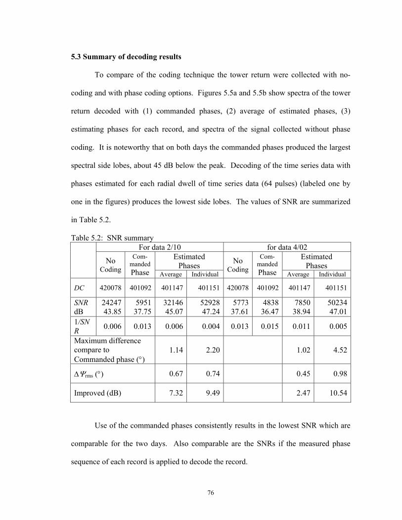
76

5.3 Summary of decoding results

To compare of the coding technique the tower return were collected with no-

coding and with phase coding options. Figures 5.5a and 5.5b show spectra of the tower

return decoded with (1) commanded phases, (2) average of estimated phases, (3)

estimating phases for each record, and spectra of the signal collected without phase

coding. It is noteworthy that on both days the commanded phases produced the largest

spectral side lobes, about 45 dB below the peak. Decoding of the time series data with

phases estimated for each radial dwell of time series data (64 pulses) (labeled one by

one in the figures) produces the lowest side lobes. The values of SNR are summarized

in Table 5.2.

Table 5.2: SNR summary For data 2/10 for data 4/02

Estimated Phases

Estimated Phases

No Coding

Com- manded Phase Average Individual

No Coding

Com- manded Phase Average Individual

DC 420078 401092 401147 401151 420078 401092 401147 401151

SNR dB

24247 43.85

5951 37.75

3214645.07

5292847.24

577337.61

483836.47

7850 38.94

5023447.01

1/SNR 0.006 0.013 0.006 0.004 0.013 0.015 0.011 0.005

Maximum difference compare to Commanded phase (°)

1.14 2.20 1.02 4.52

∆Ψrms (°) 0.67 0.74 0.45 0.98

Improved (dB) 7.32 9.49 2.47 10.54

Use of the commanded phases consistently results in the lowest SNR which are

comparable for the two days. Also comparable are the SNRs if the measured phase

sequence of each record is applied to decode the record.

77

-30 -20 -10 0 10 20 30

-20

-10

0

10

20

30

40

50

Velocity (ms-1)

Pow

er (d

B)

No CodingCommandedEstimatedEstimated one by one

-30 -20 -10 0 10 20 30

-10

0

10

20

30

40

50

60

Velocity (ms-1)

Pow

er (d

B)

No CodingCommandedEstimatedEstimated one by one

Figure 5.5: Power spectra of sequences decoded using various phase estimates. Top plots show spectra for tower 2/10, bottom plots show spectra for tower 4/02.

2/10

4/02

78

This is expected as such individual correction may compensate for some propagation

effects. Improvements in the SNR with respect to the lowest values (obtained with

commanded phases) for the two days are listed in the last row of Table 5.2. The phase

shifter is stable. The reasons for significant difference in the SNRs between the two

days and for the cases where there was no phase coding and when the average of

estimates was used are not known. The fact that individually measured (over the record

equal to the code length of 64 samples) phases gives the best SNR suggests that

instantaneous sampling of the phase of the transmitted signal (such as done by the RVP-

8 processor, Sigmet) might be the best solution.

5.4 Conclusion

The ground clutter return was used to test the overall phase stability of the radar

as well as the quality of phase shifter. Because phase shifting is required for generation

of systematic codes to mitigate range and velocity ambiguities, it was important to

determine phases of the existing phase shifter. Reported test and spectral analysis

demonstrated that the phase shifter is stable, but the realized phases differ

systematically although slightly from the commanded phases. It was demonstrated that

the ground clutter return can be used to determine exact phases for decoding that allow

accomplishing up to 10 dB of SNR improvement. For the NEXRAD system the ground

clutter returns obtained with a stationary antenna can be used to test the overall phase

stability thus calibrating the radar and improving SNR.

79

6. Concluding remarks

6.1 Summary

This thesis investigates echo and spectral signatures of non-meteorological point

scaterrers, particularly airplanes, birds, and ground clutter in the planetary boundary

layer (PBL). It is determined that

Airplanes

can be distinguished by their spectra, due to unique features corresponding to

the physical specifications of each craft;

can be tracked by weather radars.

Spectral signatures of birds

are evident even in the background wind;

can be used to recognize and track isolated birds at close ranges;

can be used for correcting bird-contaminated wind profiles;

do not depict the wing beating frequency.

Spectral signatures of ground clutter

can be used to determine phases for decoding phase-coded data, allowing up to

10 dB SNR improvement;

can be used to to test overall phase stability for calibrating radar.

6.1.1. Airplanes

An airplane has features in its spectra corresponding to the physical

specifications of the craft. Categories of airplanes (e.g. with or without a propeller,

large or small) could be distinguished by their spectra. The simple model of an airplane

80

demonstrated a decent prediction of target characteristics. The TWS (track while scan)

systems could probably avoid confusion caused by crossing target tracks by adding a

procedure that examines spectral signatures which could possibly be associated with

each individual aircraft.

Tracking a small airplane in PBL demonstrated the possibility for detection and

application of weather radar for tracking non-cooperative planes. The tracking can be

done using rapid consecutive scan. The airplane was easy to detect in both spectra and

PPI at close ranges. Nonetheless tracking at WSR-88D volume updates rates (~5 min)

might be difficult and will need association from volume scan to volume scan and might

confuse airplanes with large birds or moving automobiles (from side lobe).

6.1.2 Birds

The hypothesis that a signature of beating wings would appear as a shouldered

sidelobe on the bird spectra was not confirmed. The simulation demonstrated that only

wing-beating frequency more then 8 Hz would be distinguishable.

Large solitary birds (e.g. hawk) isolated in flight at close ranges (about 7 km)

were tracked over a considerably long period of time 2.5 minutes (rapid consecutive

scan). Bird spectral signatures are evident even in the background wind, some time

ground clutter, and noise. Nocturnal (e.g. passerine) birds covering 30 km range so that

every resolution volume had one or few birds in it (sometimes none) were observed,

and distinguished from the wind and clutter (Section 4.3).

The simple model of a bird verified the understanding of bird flight and body

characteristics. Bird signatures can be observed in spectra and therefore, might be

81

removed with appropriate filtering techniques from the weather signals, or separated

and amplified for observing bird behavior in ornithological studies.

6.1.3. Ground Clutter

A strong point ground clutter signal can serve for the radar calibration, and

effective SNR improvement. The phase coded echo from a stationary point scatterer

was examined to determine uncertainties in radar oscillator phase. The determined

phases were used for decoding phase-coded data, allowing up to 10 dB SNR

improvement.

6.2 Further Work

Outlining further work I would like to emphasize the importance of spectral

analysis and the necessity to correctly identify spectral signatures for improving the

interpretation of signals and procedures for data censoring. The following ideas for

future work come to mind.

1. Constructing an algorithm for distinguishing and tracking airplanes with weather

radars.

2. Building the airplane signatures bank.

3. Creating a filtering-enhancing technique based on the obtained spectral

information, for example, a technique for correcting bird-contaminated wind

profiles.

4. Spectral analysis of bird signatures needs to be supported by the ornithological

data and actual observation that will help completely understand the phenomena.

5. A strong point ground clutter (e.g. radio tower) return should be investigated in

different wind conditions for its vibration signature.

82

Bibliography

[1] Achtemeier G. L., 1990: The Use of Insects as Tracers for “Clear-Air” Boundary-Layer Studies by Doppler Radar. J. Atmos. Ocean. Tech., Vol. 8, pp. 746-765.

[2] Battan, L. J., 1973: Radar Observations of the Atmosphere. University of

Chicago Press, 324 pp.

[3] Doviak, R. J. and D. S. Zrnić, 1984: Doppler Radar and Weather Observations. Academic Press, 458 pp.

[4] Doviak, R. J. and D. S. Zrnić, 1984: Matched Filter Criteria and Range

Weighting for Weather Radar. IEEE Vol. AES-14, 6, 925-930. [5] Campistron, B., 1975: Characteristic distributions of angel echoes in the lower

atmosphere and their meteorological implications. Boundary-Layer Meteorology 9: 411-426.

[6] Larkin R.P., W.R. Evans, and R. H. Diehl, 2001: Nocturnal Flight Calls of

Dickcissels and Doppler Radar Echoes over South Texas in Spring. J. Field Ornithol. 73(1): 2-8

[7] Larkin R.P., and R. H. Diehl, 2001: Spectrum Width of Birds and Insects on

Pulsed Doppler Radar. Illinois Press, 20 pp

[8] Mueller E. A., and R. P. Larkin, 1984: Insects observed Using Dual-Polarization Radar. J. Atmos. Ocean. Tech., 2, 49-54.

[9] Mueller E. A., 1983: Differential Reflectivity of Birds and Insects. Edmonton,

Canada. Amer. Meteor. Soc.

[10] Sachidananda, M. and D. S. Zrnić, 1999: Systematic Phase Codes for Resolving Range Overlaid Signals in a Doppler Weather Radar. J. Atmos. Ocean. Tech., 16, 1351-1364.

[11] Vaughn C. R., 1985: "Birds and insects as radar targets: A review," Proc. IEEE,

73, 205-227, Feb. 1985.

[12] Riley J. R., 1985: "Radar cross section of insects," Proc. IEEE, 73, 228-232, Feb.1985

[13] Rabin, R. M., R. J. Doviak, 1989: Meteorological and astronomical influences

on radar reflectivity in the convective boundary layer. J. Appl. Meteor., 28, 1226-1235

83

[14] Wilczak J. M., R. G. Strauch, F. M. Ralph, B. L. Weber, D. A. Merrit, J. R. Jordan, D. E. Wolf, L. K. Lewis, D. B. Wuertz, J. E. Gaynor, S. A. McLaughlin, R. R. Rogers, A. C. Riddle, and T.S. Dye 1995: Contamination of wind profiler data by migrating birds: Characteristics of corrupted data and potential solutions, J. Atmos. Ocean. Tech., 12, 449-467.

[15] Wilson, J. W., Weckwerth, T. M., Vivekanandan, J., Wakimoto, R. M., Russell,

R.W., 1994: Boundary layer clear-air radar echoes: origin of echoes and accuracy of derived winds. J. Atmos. Ocean. Tech. 11:1184-1206.

[16] Zrnić D. S, and A. V. Ryzhkov, 1998: Observation of Insects and Birds with

Polarimetric Radar. IEEE Trans. Geosci. Remote Sens., 36, No. 2, 661-668. [17] Zrnić D. S, and Mahapatra 1985: Two methods of ambiguity resolution in

pulsed Doppler weather radars. IEEE Trans. Aerospace Electr. Syst., 21, 470-483

[18] Zrnić D. S, and M. Sachidananda, 1986: Recovery of spectral moments from

overlaid echoes in a Doppler weather radar. IEEE Trans. Geosci. Remote Sens., 24, 751-764

[19] Personal communications with Zrnić D. S, September 2003.

84

Appendix Table A1: Data 2/10. The phases, their difference, and the standard deviation for the tower

1 2 3 4 5 k Commanded Phase

(degrees) Estimated Phase (degrees)

Difference [3]-[2] (degrees)

Standard Deviation (degrees)

1 2 3 4 5 6 7 8 9 10 11 12 13 14 15 16 17 18 19 20 21 22 23 24 25 26 27 28 29 30 31 32 33 34 35 36 37 38 39 40 41 42 43 44 45 46 47 48 49 50 51 52 53 54 55 56 57 58 59 60 61 62 63 64

0 -22.5 -112.5 45.0 45.0 -157.5 112.5 90.0 90.0 67.5 -22.5 135.0 135.0 -67.5 -157.5 180.0 180.0 157.5 67.5 -135.0 -135.0 22.5 -67.5 -90.0 -90.0 -112.5 157.5 -45.0 -45.0 112.5 22.5 0 0 -22.5 -112.5 45.0 45.0 -157.5 112.5 90.0 90.0 67.5 -22.5 135.0 135.0 -67.5 -157.5 180.0 180.0 157.5 67.5 -135.0 -135.0 22.5 -67.5 -90.0 -90.0 -112.5 157.5 -45.0 -45.0 112.5 22.5 0

0 -21.5447 -112.4008 45.0811 45.0203 -158.4123 111.9415 89.8464 89.8114 67.9936 -21.4976 134.4742 134.4190 -66.5753 -158.4108 178.9186 178.8632 156.8656 68.0014 -135.3065 -135.3887 22.5191 -66.5941 -88.9298 -88.9571 -112.4027 156.9293 -44.0539 -44.0982 112.0190 22.5154 0.0237 0.0226 -21.5263 -112.4115 45.0769 45.0144 -158.4388 111.9217 89.8152 89.8135 67.9805 -21.4864 134.4600 134.4071 -66.5765 -158.3987 178.9430 178.8859 156.9017 68.0369 -135.2968 -135.3857 22.5291 -66.5886 -88.9195 -88.9111 -112.3874 156.9397 -44.0765 -44.1269 111.9904 22.4851 0.0042

0 0.9553 0.0992 0.0811 0.0203 -0.9123 -0.5585 -0.1536 -0.1886 0.4936 1.0024 -0.5258 -0.5810 0.9247 -0.9108 -1.0814 -1.1368 -0.6344 0.5014 -0.3065 -0.3887 0.0191 0.9059 1.0702 1.0429 0.0973 -0.5707 0.9461 0.9018 -0.4810 0.0154 0.0237 0.0226 0.9737 0.0885 0.0769 0.0144 -0.9388 -0.5783 -0.1848 -0.1865 0.4805 1.0136 -0.5400 -0.5929 0.9235 -0.8987 -1.0570 -1.1141 -0.5983 0.5369 -0.2968 -0.3857 0.0291 0.9114 1.0805 1.0889 0.1126 -0.5603 0.9235 0.8731 -0.5096 -0.0149 0.0042

0 0.9715 0.2268 0.2231 0.2124 0.9307 0.6130 0.3178 0.3143 0.5508 1.0250 0.5919 0.6464 0.9724 0.9536 1.1069 1.1770 0.7031 0.5848 0.4071 0.4643 0.2909 0.9549 1.1082 1.0714 0.2450 0.6324 0.9916 0.9469 0.5570 0.2738 0.3144 0.3281 1.0189 0.3150 0.2941 0.3234 1.0009 0.6772 0.3973 0.3930 0.6320 1.0925 0.6614 0.6957 0.9878 0.9699 1.1221 1.1809 0.7130 0.6566 0.5187 0.5786 0.4014 0.9872 1.1516 1.1587 0.4264 0.6939 1.0064 0.9581 0.6679 0.4469 0.4309

rms . 0.67 0.74

85

Table A2: Data 4/02. The phases, their difference, and the standard deviation for the tower

1 2 3 4 5

k Commanded Phase (degrees)

Estimated Phase (degrees)

Difference [3]-[2] (degrees)

Standard Deviation (degrees)

1 2 3 4 5 6 7 8 9

10 11 12 13 14 15 16 17 18 19 20 21 22 23 24 25 26 27 28 29 30 31 32 33 34 35 36 37 38 39 40 41 42 43 44 45 46 47 48 49 50 51 52 53 54 55 56 57 58 59 60 61 62 63 64

0 -22.5

-112.5 45.0 45.0

-157.5 112.5 90.0 90.0 67.5

-22.5 135.0 135.0 -67.5

-157.5 180.0 180.0 157.5 67.5

-135.0 -135.0

22.5 -67.5 -90.0 -90.0

-112.5 157.5 -45.0 -45.0 112.5 22.5

0 0

-22.5 -112.5

45.0 45.0

-157.5 112.5 90.0 90.0 67.5

-22.5 135.0 135.0 -67.5

-157.5 180.0 180.0 157.5 67.5

-135.0 -135.0

22.5 -67.5 -90.0 -90.0

-112.5 157.5 -45.0 -45.0 112.5 22.5

0

0 -21.6502 -112.5322 44.9247 44.8409

-158.3160 111.8618 89.6101 89.5985 67.9115 -21.5697 134.6499 134.6559 -66.6952 -158.2264 179.4035 179.3872 157.5204 67.9358

-135.3983 -135.5324 22.4569 -66.7793 -88.9767 -89.0676 -112.4897 157.5255 -44.1145 -44.1513 111.9338 22.4896 0.0712 0.0720

-21.6160 -112.4401 44.9536 44.9263

-158.3122 111.8961 89.6116 89.5824 67.9500 -21.5791 134.6690 134.5944 -66.7499 -158.3387 179.3656 179.3462 157.5235 67.9379

-135.4104 -135.4908 22.4261 -66.7692 -89.0160 -89.0271 -112.5126 157.5697 -44.1322 -44.1961 111.8796 22.4296 0.0624

0 0.8498 -0.0322 -0.0753 -0.1591 -0.8160 -0.6382 -0.3899 -0.4015 0.4115 0.9303 -0.3501 -0.3441 0.8048 -0.7264 -0.5965 -0.6128 0.0204 0.4358 -0.3983 -0.5324 -0.0431 0.7207 1.0233 0.9324 0.0103 0.0255 0.8855 0.8487 -0.5662 -0.0104 0.0712 0.0720 0.8840 0.0599 -0.0464 -0.0737 -0.8122 -0.6039 -0.3884 -0.4176 0.4500 0.9209 -0.3310 -0.4056 0.7501 -0.8387 -0.6344 -0.6538 0.0235 0.4379 -0.4104 -0.4908 -0.0739 0.7308 0.9840 0.9729 -0.0126 0.0697 0.8678 0.8039 -0.6204 -0.0704 0.0624

0 1.0168 0.8747 0.9080 1.0216 1.1928 0.8921 0.7225 0.9218 1.0932 1.3523 1.0598 0.8732 0.9891 1.0485 1.1815 1.2441 1.0694 1.0265 0.8502 0.7974 0.8598 1.3241 1.4689 1.4246 0.7895 0.6232 1.0925 1.2340 1.1560 1.0692 1.0482 0.8603 1.0813 0.7932 0.9936 1.0499 1.3720 1.1900 0.8695 0.7221 0.9156 1.3501 1.1045 1.1461 1.1810 1.1453 0.9764 1.1105 0.9635 1.1017 0.9962 0.9109 0.5446 1.0182 1.3502 1.4073 1.0583 0.9504 1.2019 1.1101 1.1339 1.0875 1.0493

rms 0.57 1.06

86

Table A3: Summary for data 2/10 and 4/02. Phases are in degrees.

1 2 3 4 5 k Commanded Phase

(degrees)

Estimated Phase 030210

(degrees)

Estimated Phase 030402

(degrees)

Difference [3]-[4]

(degrees) 1 2 3 4 5 6 7 8 9

10 11 12 13 14 15 16 17 18 19 20 21 22 23 24 25 26 27 28 29 30 31 32 33 34 35 36 37 38 39 40 41 42 43 44 45 46 47 48 49 50 51 52 53 54 55 56 57 58 59 60 61 62 63

64

0 -22.5

-112.5 45.0 45.0

-157.5 112.5 90.0 90.0 67.5

-22.5 135.0 135.0 -67.5

-157.5 180.0 180.0 157.5 67.5

-135.0 -135.0

22.5 -67.5 -90.0 -90.0

-112.5 157.5 -45.0 -45.0 112.5 22.5

0 0

-22.5 -112.5

45.0 45.0

-157.5 112.5 90.0 90.0 67.5

-22.5 135.0 135.0 -67.5

-157.5 180.0 180.0 157.5 67.5

-135.0 -135.0

22.5 -67.5 -90.0 -90.0

-112.5 157.5 -45.0 -45.0 112.5 22.5

0

0 -21.5447

-112.4008 45.0811 45.0203

-158.4123 111.9415 89.8464 89.8114 67.9936

-21.4976 134.4742 134.4190 -66.5753

-158.4108 178.9186 178.8632 156.8656 68.0014

-135.3065 -135.3887

22.5191 -66.5941 -88.9298 -88.9571

-112.4027 156.9293 -44.0539 -44.0982 112.0190 22.5154 0.0237 0.0226

-21.5263 -112.4115

45.0769 45.0144

-158.4388 111.9217 89.8152 89.8135 67.9805

-21.4864 134.4600 134.4071 -66.5765

-158.3987 178.9430 178.8859 156.9017 68.0369

-135.2968 -135.3857

22.5291 -66.5886 -88.9195 -88.9111

-112.3874 156.9397 -44.0765 -44.1269 111.9904 22.4851 0.0042

0 -21.6502 -112.5322 44.9247 44.8409

-158.3160 111.8618 89.6101 89.5985 67.9115 -21.5697 134.6499 134.6559 -66.6952 -158.2264 179.4035 179.3872 157.5204 67.9358

-135.3983 -135.5324 22.4569 -66.7793 -88.9767 -89.0676 -112.4897 157.5255 -44.1145 -44.1513 111.9338 22.4896 0.0712 0.0720

-21.6160 -112.4401 44.9536 44.9263

-158.3122 111.8961 89.6116 89.5824 67.9500 -21.5791 134.6690 134.5944 -66.7499 -158.3387 179.3656 179.3462 157.5235 67.9379

-135.4104 -135.4908 22.4261 -66.7692 -89.0160 -89.0271 -112.5126 157.5697 -44.1322 -44.1961 111.8796 22.4296 0.0624

0 0.1055 0.1313 0.1564 0.1794 -0.0963 0.0797 0.2362 0.2129 0.0821 0.0721 -0.1757 -0.2368 0.1199 -0.1844 -0.4849 -0.5240 -0.6548 0.0656 0.0918 0.1436 0.0621 0.1852 0.0469 0.1105 0.0871 -0.5962 0.0606 0.0532 0.0852 0.0258 -0.0475 -0.0494 0.0897 0.0285 0.1233 0.0880 -0.1266 0.0256 0.2036 0.2311 0.0305 0.0928 -0.2090 -0.1873 0.1733 -0.0600 -0.4226 -0.4603 -0.6217 0.0990 0.1136 0.1052 0.1030 0.1806 0.0965 0.1160 0.1251 -0.6300 0.0557 0.0692 0.1108 0.0555 -0.0582

rms 0.23