analyze frequency response (bode plots) with r&s ... · analyze frequency response (bode plots)...

Analyze Frequency Response (Bode Plots) with R&S Oscilloscopes Application Note

Products:

ı R&S®RTO2002

ı R&S®RTO2012

ı R&S®RTO2022

ı R&S®RTO2044

ı R&S®RTO2004

ı R&S®RTO2014

ı R&S®RTO2024

ı R&S®RTO2064

This application note describes how to use the R&S RTO oscilloscopes for gain and phase measurements

(Bode plots) on active and passive single-ended 2-port circuits.

Note:

Please find the most up-to-date document on our homepage http://www.rohde schwarz.com/appnote/1TD07

This document is complemented by software. The software may be updated even if the version of the

document remains unchanged

App

licat

ion

Not

e

M. W

ollin

ger,

J. G

anze

rt

11.2

017 –

1TD

07_1

e

http://www.rohde-schwarz.com/appnote/1TD07

Table of Contents

1TD07_1e Rohde & Schwarz Analyze Frequency Response (Bode Plots) with R&S Oscilloscopes

2

Table of Contents

1 Overview .............................................................................................. 3

2 Features ............................................................................................... 4

2.1 Functionalities .............................................................................................................. 4

2.1.1 Measurements ............................................................................................................... 4

2.1.2 Results Documentation .................................................................................................. 5

2.2 Benefit of an Oscilloscope-based solution ............................................................... 5

2.2.1 Non 50 Ohm condition ................................................................................................... 5

2.2.2 Frequency Range down to DC ...................................................................................... 5

3 Application Examples......................................................................... 6

4 Hardware Configuration ..................................................................... 7

5 Installation Guide ................................................................................ 8

5.1 Installation on the Oscilloscope RTO ........................................................................ 8

5.1.1 Installation Step by Step ................................................................................................ 8

5.1.2 Attach Icon to the App Cockpit ...................................................................................... 8

5.2 Installation on a Separate Computer .......................................................................10

5.2.1 Installation location ......................................................................................................10

5.2.2 Launching the application ............................................................................................10

6 Example Measurement of a Low Pass Filter .................................. 11

6.1 Measurement Setup ...................................................................................................11

6.2 Measurement Procedure ...........................................................................................14

6.3 Measurement Results ................................................................................................15

7 Parameter Description with Ranges................................................ 20

8 Literature ........................................................................................... 21

9 Ordering Information ........................................................................ 22

Overview


3

1 Overview

Analyzing the frequency response of active or passive components and modules is the

typical application for network analyzers. However, these specialized instruments

typically do not support measurements close to DC signals. Moreover, they mostly

require 50-Ohm impedance.

This application note describes a software supported oscilloscope-based solution,

which addresses some of the above shortcomings:

ı Not bound to 50-Ohm reference impedance.

ı Lower frequency limit is 0 Hz.

ı Oscilloscope probes impose only small loading on the circuit.

The results are frequency response diagrams in magnitude and phase, also known as

Bode plots.

Surely, this approach also has some limitations:

ı Measurement accuracy is limited due to simple error correction mechanism (no

full two-port error correction like on a vector network analyzer).

ı Frequency range determined by oscilloscope bandwidth and function generator,

which is typically lower than on a vector network analyzer.

Features


4

2 Features

2.1 Functionalities

The low frequency network analyzer application allows you to characterize the

frequency response of a 2-port circuit. This can be a passive component (filter,

attenuator, cable) or an active component (amplifier).

It is very common to move the reference plane for the measurements to the connectors

of the DUT. On network analyzers, this task is called calibration or system error

correction. This application also provides a simplified calibration. The software allows

you to correct for phase and gain response of the cabling by means of a normalization.

2.1.1 Measurements

The present application allows measuring the following characteristics:

ı Gain response

ı Phase response

The most common measurement is the gain behavior over frequency. For filter

components, the gain should be flat in the pass-band. The roll-off behavior is also

important, because it influences the settling behavior (rise time, overshoot, ringing) of

digital signals.

Fig. 2-1: Gain response of a low pass filter

Phase behavior over frequency is equally substantial. In the pass-band, the ideal

phase behavior is linear over frequency.

Features


5

Fig. 2-2: Phase response of a low-pass filter

Note that phase wrapping is always enabled in this software.

2.1.2 Results Documentation

Documenting the measurements is always an important part of the analysis. This

application offers the following features:

ı Linear / logarithmic display of the frequency axis

Note that the interval between frequency points is always linear.

ı Save measurement to memory for direct comparison on the screen

ı Save trace data to file

ı Up to 4 markers

In addition, the display includes some useful status information (calibration valid; count

of traces in memory).

2.2 Benefit of an Oscilloscope-based solution

2.2.1 Non 50 Ohm condition

Dedicated network analyzers are limited to a certain reference impedance. This is

typically 50 Ohm, sometimes 75 Ohm. For any other impedance, transformers are

required.

The oscilloscope-based solution offers the advantage that probes have typically a high

input impedance and thus impose only a small loading onto the DUT.

2.2.2 Frequency Range down to DC

Network analyzers typically use directional couplers to measure all 4 S-parameters of a

two-port module. Depending on the architecture of the couplers, they have a lower

frequency limit of 9 kHz and higher. This means that frequency response

measurements cannot be done below this limit. The oscilloscope on the contrary can

do measurements starting at DC. This can be a significant advantage.

Application Examples


6

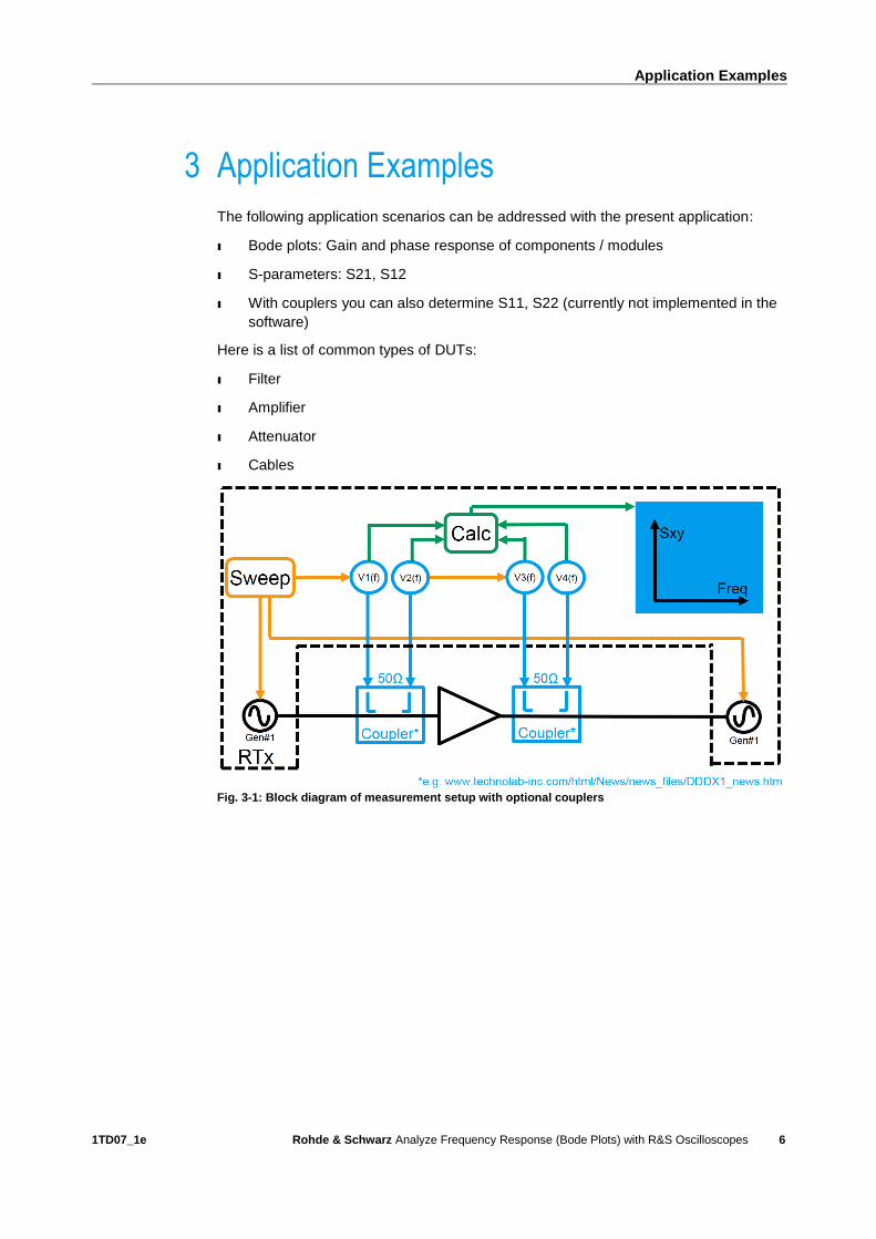
3 Application Examples

The following application scenarios can be addressed with the present application:

ı Bode plots: Gain and phase response of components / modules

ı S-parameters: S21, S12

ı With couplers you can also determine S11, S22 (currently not implemented in the

software)

Here is a list of common types of DUTs:

ı Filter

ı Amplifier

ı Attenuator

ı Cables

Fig. 3-1: Block diagram of measurement setup with optional couplers

Hardware Configuration


7

4 Hardware Configuration

The following components are required for the application described in this document:

Oscilloscope:

RTO2000

Hardware options: Arbitrary waveform generator RTO-B6

Software options: RTO-K11 (IQ data software interface)

Probes:

All available probes can be used (passive and active probes)

Installation Guide


8

5 Installation Guide

5.1 Installation on the Oscilloscope RTO

5.1.1 Installation Step by Step

The application comes in a standalone executable file LFNWA.exe, which launches the

Low Frequency Network Analyzer. The executable file does require installation; simply

save it in a location of your choice on the instrument's internal hard drive. We

recommend saving the executable file in a reasonable location, like a separate folder

on the desktop or in the program files directory.

5.1.2 Attach Icon to the App Cockpit

The user interface of the RTO2000 allows inserting custom applications to the app

cockpit. This facilitates their launch and enhances the user-friendly environment. In

order to add the Low Frequency Network Analyzer application to the App Cockpit into

the section User Apps, execute the following steps:

ı Click on the menu button to open the App Cockpit

ı Change to the User Apps tab in the App Cockpit (Fig. 5-1).

Fig. 5-1: App Cockpit with the tab "User Apps"

ı Click the "Add tool" button (Fig. 5-1) to add the desired user-defined tool shortcut

to the tab.

ı Enter the desired tool name, for example LFNWA (Low Frequency Network

Analyzer) into the first textbox. (Fig. 5-2). This indication will appear later as a

description below the application icon.

Installation Guide


9

ı Select an appropriate image by entering the path to the icon file in the respective

line. Click on the "…" button to open a popup window where you select the path to

the icon file. You can find a suitable icon file in the installation package.

Now select the executable file by clicking on the "…" button in the "Select tool:" line.

ı This application does not require arguments, so leave the respective field empty.

ı Click the "test run" to verify if the application starts correctly. (Fig. 5-2)

ı Finally click the "Add tool" button to complete the process (Fig. 5-3). The shortcut

is now visible in the App Cockpit and you can launch the application from here.

Fig. 5-3: Shortcut of the LFNWA application in the "User Apps" tab

Fig. 5-2: Input box to add the shortcut

Installation Guide


10

5.2 Installation on a Separate Computer

5.2.1 Installation location

Beside the deployment of the application on the oscilloscope itself, it is also possible to

run the Low Frequency Network Analyzer on a separate computer.

The installation is identical to the installation on the oscilloscope. The distributed

executable file, LFNWA.exe, should be located in a reasonable location. To launch the

application, the executable simply double click on the respective icon.

5.2.2 Launching the application

Starting the application from the computer requires an additional step. You must first

establish a connection to the oscilloscope. At the launch of the executable file, a pop-

up window requests the IP address of the device. You can enter the computer name

(hostname) of the oscilloscope as well as the IP address. The application terminates

automatically, upon entering an incorrect IP address or connection failure. For a

second try, restart the executable file LFNWA.exe.

Example Measurement of a Low Pass Filter


11

6 Example Measurement of a Low Pass Filter

6.1 Measurement Setup

The characterization of a low pass filter will clarify the measurement procedure and its

setup.

Connect the measurement points of the DUT channel 1 and 2 of the oscilloscope. Note

that the measuring probe of channel 1 shall be connected exclusively to the input port

of the DUT and the probe of channel 2 to the output port of the DUT (Fig. 6-1). This is

due to the assumption of the application that channel 1 measures the signal at input

side and channel 2 on output side.

Fig. 6-1: Connection of the oscilloscope channels for S21 measurement

Fig. 6-2: ARB signal generator output on the rear panel

In order to measure the S21 forward transmission parameter, a sine wave from the

internal generator of the oscilloscope is applied to the DUT. The output of the DUT



12

shall be terminated with the matching impedance of the DUT (typically 50 ohms) to

avoid reflections.

The output Gen 1 of the RTO-B6 option at the back of the oscilloscope is connected to

port 1 of the DUT with a BNC cable. Output Gen 2 can also be used; in this case, the

setting needs to be adapted in the menu of the user interface of the application. Port 2

of the DUT is terminated with a 50-Ohm resistor.

The various parameters for the measurement are entered in the user interface. The

default arguments are displayed in Fig. 6-3. For the characterization of the example

low pass filter, the frequency should sweep from 20 MHz to 50 MHz. Set the start

frequency by clicking on the button, which displays the current frequency setting. A

popup window (Fig. 6-4) enables you to insert the required value and to confirm the

input with the according unit button. A step frequency of 1 MHz is a reasonable value

for this measurement range.



13

Fig. 6-3: Configuring the measurement parameters

Fig. 6-4: Setting the Start Frequency

The level of 0 dBm is also suitable for the low pass filter measurement. The correct

input power depends on the characteristics of the DUT. For passive components

(filters, attenuators) it must be sufficient to provide a signal at the output that is well

above the noise floor in the passband. For amplifiers, it must be sufficiently low at the

amplifier input to avoid saturation of the DUT. The dBm values are referenced to the

underlying 50-Ohm system.

Select the bandwidth from a drop down list. This parameter is crucial for the frequency

resolution of the measurement. With a frequency range in the MHz region, the default

bandwidth of 10 kHz is a good choice.

The average factor applies to each individual measurement point. A higher average

count implies that the data is acquired multiple times at each frequency point and

averaged, before displayed on the plot. Averaging has a similar effect like filtering.



14

6.2 Measurement Procedure

Start the measurement after all settings are completed. However, depending on the

connection setup of the DUT a calibration step may be useful or even required.

For the calibration / normalization step, insert a through connection instead of the DUT.

Start the calibration by clicking on the CAL button in the measurement group (Fig. 6-5).

Fig. 6-5: Measurement section

During the calibration process, the system collects data that characterizes the

frequency response outside the DUT thus compensating unwanted effects in cabling

and connectors. The calibration procedure will display a dotted trace, and display the

valid range of the accomplished calibration in the "Info" section on the user interface

(Fig. 6-7).

Modifying the frequency range (start and stop frequency) results in cancellation of the

calibration.

Fig. 6-6: Info section



15

Fig. 6-7: Dotted graph displays the calibration

After performing the calibration, connect the DUT to the measurement setup.

Start the actual measurement by clicking on the Start button in the measurement

section on the user interface (Fig. 6-5).

The trace displays the transmission function of the device under test (DUT) in the

selected frequency range. The recorded calibration values are taken into account

accordingly.

6.3 Measurement Results

The curves, displayed on the two bode plots; represent the transmission function, S21,

of the DUT. The upper graph displays the amplitude frequency response and provides

information on the amplitude behavior over the according frequency range in dB (Fig.

6-8).

Fig. 6-8: Gain response

The second plot displays the phase characteristics over frequency, measured in ° (Fig.

6-9).



16

Fig. 6-9: Phase response

You can adjust the y - axis scaling of the gain graph in the Scaling menu.

The menu section provides two scaling types for the y-axis:

ı Manual scaling: Select Scale/Div., Ref Value, and Ref Pos values manually (Fig.

6-10)

ı Auto scaling: The vertical scale is adjusted automatically such that the graph fits

entirely into the diagram.

The scale/div parameter determines the dB per division. The diagram always contains

10 divisions. The reference value and the reference position are auxiliary values to

control the configuration of the plotting area. The reference value, marked with a blue,

horizontal line, is positioned by the reference position onto a specific division. With

frequency response of the low pass filter moving close to the border of the plot, it is

good practice to adjust the scaling manually. To lower the plotted line, set the

reference position set to a smaller value, e.g. 8.

Fig. 6-10: Vertical scale setup

Similar to the vertical axis, you can adjust the scaling of the frequency (x-) axis. The

frequency axis can be displayed either in a linear or in a logarithmic scale. For the

example of the low pass filter, the linear scale configuration is sufficient.



17

For a better inspection of the frequency responses, several markers are available

under the set marker menu. Four markers can be activated via a pop-up window.

Fig. 6-11: Marker Settings

Set the frequency position of the several markers by clicking on the button and

entering the desired frequency value. Alternatively, you can drag the marker to the

desired position, directly on the plotted trace. A legend appears above the diagrams,

displaying the corresponding coordinates of the markers. To determine the cutoff

frequency of the low pass filter, you can activate two markers. The cutoff frequency is

defined as the frequency for which the output of the circuit is 3 dB below the nominal

passband value. To consider this condition, place marker 1 at the nominal passband,

and marker 2, 3 dB below marker 1. The marker info facilitates finding the exact

position of the cutoff frequency and determine the frequency value of 24.26 MHz (Fig.

6-12).



18

Fig. 6-12: Marker measurements

In order to compare the recoded transmission function with a transmission function

from another device, the Data to Memory button (Data Mem) in the measurement

region saves the current trace to a local memory. For comparison, the second DUT

must be inserted into the measurement setup and measured. The local data will be

plotted concurrently. You can compare several traces with this feature.

The following figure 6-10 displays the comparison of the low pass filter of the example,

and a high pass filter with a cut off frequency at the same frequency. The red, dotted

trace represents the local stored frequency response of the low pass filter. The high

pass filter frequency response got loaded by the menu option, read data from file.



19

Fig. 6-13: Comparing a low-pass filter and a high-pass filter

Another benefit of this option is shown in Fig. 6-14. The red-dotted race displays the

locally saved low pass filter. The new measured trace is the same filter with an in

series connected attenuator. It can be observed that the additional component

attenuates the amplitude frequency response by 10 dB.

Fig. 6-14: Low-pass filter with additional attenuator

Parameter Description with Ranges


20

7 Parameter Description with Ranges

Parameter Description Range

Start Frequency upper range limited by current Stop Frequency

1Hz to 100MHz

Stop Frequency lower range limited by current Start Frequency

1 Hz to 100 MHz

Step Frequency Linear interval between frequency points

1 Hz to 100 MHz

Level ARB generator output level (=DUT input level)

-35dBm to 19dBm

Bandwidth Filter bandwidth 1kHz, 2kHz, 4kHz, 5kHz, 10kHz, 20kHz, 40kHz, 50kHz, 100kHz

Average Averaging factor for point average at each frequency point

Integer value from 1 to 1000

Scale per division

Vertical scale 0.5 dB/div to 20 dB/div

Reference Value

Vertical reference value -100 dB to 100 dB

Reference Position

Vertical reference position 0 to 10

Literature


21

8 Literature

[1] <Autor> <Title> (Enter Bibliography via >R&S Manual!Figure+Tools >Manage

Bibliography Sources, In dialog: activate "Show All Bibliography Fields" to enter

hyperlinks) [Book Section]. - <Year>.

Ordering Information


22

9 Ordering Information

Naming Type Order number

Digital Oscilloscopes

600 MHz, 2 channels

10 Gsample/s, 50/100 Msample

R&S®RTO2002 1329.7002.02

600 MHz, 4 channels


R&S®RTO2004 1329.7002.04

1 GHz, 2 channels


R&S®RTO2012 1329.7002.12

1 GHz, 4 channels


R&S®RTO2014 1329.7002.14

2 GHz, 2 channels


R&S®RTO2022 1329.7002.22

2 GHz, 4 channels


R&S®RTO2024 1329.7002.24

3 GHz, 2 channels


R&S®RTO2032 1329.7002.22

3 GHz, 4 channels


R&S®RTO2034 1329.7002.24

4 GHz, 4 channels

10 Gsample/s, 50/200 Msample 20 Gsample/s, 50/100 Msample

R&S®RTO2044 1329.7002.44

6 GHz, 4 channels

10 Gsample/s, 50/200 Msample 20 Gsample/s, 50/100 Msample

R&S®RTO2064 1329.7002.64

Hardware Options

Arbitrary Waveform Generator R&S®RTO-B6 1329.7054.02

Software Options

I/Q Software Interface R&S®RTO-K11 1317.2975.02

Rohde & Schwarz

The Rohde & Schwarz electronics group offers

innovative solutions in the following business fields:

test and measurement, broadcast and media, secure

communications, cybersecurity, radiomonitoring and

radiolocation. Founded more than 80 years ago, this

independent company has an extensive sales and

service network and is present in more than 70

countries.

The electronics group is among the world market

leaders in its established business fields. The

company is headquartered in Munich, Germany. It

also has regional headquarters in Singapore and

Columbia, Maryland, USA, to manage its operations

in these regions.

Regional contact

Europe, Africa, Middle East +49 89 4129 12345 [email protected] North America 1 888 TEST RSA (1 888 837 87 72) [email protected] Latin America +1 410 910 79 88 [email protected] Asia Pacific +65 65 13 04 88 [email protected]

China +86 800 810 82 28 |+86 400 650 58 96 [email protected]

Sustainable product design

ı Environmental compatibility and eco-footprint

ı Energy efficiency and low emissions

ı Longevity and optimized total cost of ownership

This application note and the supplied programs

may only be used subject to the conditions of use

set forth in the download area of the Rohde &

Schwarz website.

R&S® is a registered trademark of Rohde & Schwarz GmbH & Co.

KG; Trade names are trademarks of the owners.

Rohde & Schwarz GmbH & Co. KG

Mühldorfstraße 15 | 81671 Munich, Germany

Phone + 49 89 4129 - 0 | Fax + 49 89 4129 – 13777

www.rohde-schwarz.com

PA

D-T

-M: 3573.7

380.0

2/0

2.0

5/E

N/

mailto:[email protected]





analyze frequency response (bode plots) with r&s ... · analyze frequency response (bode plots)...

Documents