associative cellular learning automata and its applicationssharif.edu/~beigy/docs/2017/atb17.pdf ·...

Associative Cellular Learning Automata and its Applications

Meysam Ahangaran and Nasrin Taghizadeh and Hamid Beigy

Department of Computer Engineering,Sharif University of Technology, Tehran, Iran

[email protected], {taghizadeh, beigy}@ce.sharif.edu

Abstract

Cellular learning automata (CLA) is a distributed computational model which was introduced in the last decade. This modelcombines the computational power of the cellular automata with the learning power of the learning automata. Cellular learningautomata is composed from a lattice of cells working together to accomplish their computational task; in which each cell isequipped with some learning automata. Wide range of applications utilizes CLA such as image processing, wireless networks,evolutionary computation and cellular networks. However, the only input to this model is a reinforcement signal and so it cannotreceive another input such as the state of the environment. In this paper, we introduce a new model of CLA such that each cellreceives extra information from the environment in addition to the reinforcement signal. The ability of getting an extra inputfrom the environment results in an increase in the computational power and flexibility of the model. We designed some newalgorithms for solving famous problems in pattern recognition and machine learning such as classification, clustering and imagesegmentation. All of them are based on the proposed CLA. We investigated performance of these algorithms through severalcomputer simulations. Results of the new clustering algorithm shows acceptable performance on various data sets. CLA-basedclassification algorithm gets average precision 84% on eight data sets in comparison with SVM, KNN and Naive Bayes withaverage precision 88%, 84% and 75%, respectively. Similar results are obtained for semi-supervised classification based on theproposed CLA.

Keywords: Cellular learning automata, cellular automata, learning automata, external input, clustering, classification, self-organizing map, image segmentation.

1 IntroductionSince the introduction of the cellular learning automata (CLA) [1], various types of this computational model have been inventedand each of them has been used for solving different problems. The main idea of the CLA is to combine the learning power ofthe learning automata (LA) with the computational power of the cellular automata (CA) to produce a distributed computationalmodel. Variation of this model have been used in several applications. In the rest of this section, the motivation behind the ideagiven in the paper is explained and then the contribution of this paper is presented.

1.1 MotivationCellular learning automata is a distributed model for learning behaviour of complicated systems. CLA consists of a large numberof simple identical units, which make a global complex behaviour through the interaction with each other. One can assume theseunits, which called cells, are placed nearby in a lattice structure and communicate with their neighbours. Each cell in the CLAconsists of one or more LAs. These LAs change state of the cell based on the local rule and the reinforcement signal. CLAworks as follows: at the first step each LA in each cell chooses an action based on its action probability vector. At the secondstep, the environment passes a reinforcement signal to the LAs residing in each cell on the basis of the CLA local rule. In CLA,neighbouring LAs of any cell constitute its local environment. At the third step each LA of each cell updates its internal statebased on its current state and the received reinforcement signal. This process continues until the desired behaviour is obtained.

There are several applications that use the CLA as a basic computational element. Image segmentation [2, 3], resourceallocation in mobile networks [4, 5], multi-agent systems [6], wireless sensor networks [7, 8] and numerical optimization [9, 10]are examples of such applications. However, none of the previous models can receive extra information from the environment.Indeed, the only input to each cell is a reinforcement signal; while some tasks in pattern recognition need to such ability that

1

each cell in the CLA gets more information from the environment. This information is necessary in the process of learning andcomputing.

1.2 ContributionIn the standard model of the CLA, each cell only receives a reinforcement signal. The other information about the environmentshould be encoded in the initial state of the cells, local rule or the updating algorithms of LAs. Thus, augmentation of the CLAwith the ability of receiving extra input increases flexibility and computational power of it. In this paper, a new model for CLAis proposed. The main feature of the proposed model is the ability of receiving external input from the environment. This newmodel for CLA is called associative CLA. Associative CLA can be utilized in pattern recognition tasks such as classification,semi-supervised classification, clustering and image segmentation. In this paper, an algorithm is proposed for each of these tasksto show some of the potential usage of the proposed model. Experimental results show the efficiency of the associative CLA incontrast to the similar methods.

The rest of this paper is organized as follows: In section 2, the basic concepts and equations are presented. Section 3introduces the new model of the CLA and its components. Section 4 is devoted to design of some algorithms based on theproposed model of the CLA, consisting of the clustering, image segmentation, classification and semi-supervised classification.Results of comparing the proposed algorithms with the other related algorithms are reported in section 5. Finally, section 6represent the conclusion remarks and future works.

2 BackgroundIn what follows a brief introduction to the learning automata and cellular automata are given. Next, the combination of thesemodels into the cellular learning automata is reviewed briefly.

2.1 Learning AutomataLearning Automaton (LA) is an adaptive decision-making agent which learns an optimal action out of a set of allowable actionsthrough repeated interactions with a random environment. At each step the LA chooses an action from its action set using itsaction probability distribution and applies it to the random environment. The random environment provides a stochastic response,which is called reinforcement signal, to the LA. Then the LA uses the reinforcement signal together with a learning algorithm toupdate the action probability distribution.

Various learning automata have been proposed in the literature for usage in different applications. LAs can be classified intotwo main groups: finite action-set learning automata (FALA) [11] and continuous action-set learning automata (CALA) [12, 13].In the former, the action set from which agent chooses its action is finite. This is the original model of LA. However, in somesituations the objective of learning is to find a continuous valued parameter and the value of which cannot be discretized. So inlatter, the action set corresponds to an interval over the real line. In general, there are two classes of LAs: associative LAs andnon-associative LAs. If the interaction of the LA with the environment limited to the reinforcement signal and doesn’t receiveany other input, LA belongs to the non-associative class and vice versa.

Learning automata have been used in different applications such as graph partitioning [14], cellular mobile networks [15, 16],shortest path problem [17, 18], and topology and parameter tunning of neural networks [19, 20, 21], to mention a few.

2.2 Cellular AutomataCellular Automata (CA) is a distributed computing model providing a platform for performing complex computation with thehelp of local interactions. CA is a lattice of simple identical units, called cell. When a large number of cells are put together,complex behavioural patterns can be produced through the interaction of cells with their neighbours. The state of each cell isupdated according to the current state of itself and its neighbours, based on the updating rule of the CA.

A d-dimensional CA is defined by 〈Zd ,Φ,N,F〉, where Zd is a lattice of d-tuples of integer numbers. Each cell in Zd isshown with (z1,z2, ...,zd) and Φ = {1,2, ..,k} is a finite set of cell states. N = {x1,x2, ...,xm}, which is called neighbour vector,is a finite subset of the Zd . Neighbour vector determines the relative positions of neighbouring cells for any given cell in the Zd .Neighbours of a cell u are the set {u+ xi|i = 1,2, ...,m}, and finally, F : Φm → Φ is the local rule of the CA which gives the newstate of the cell according to the current state of its neighbours.

Since its inception, different structural variations of CA have been proposed. CAs can be classified based on different features.According to the possible states for the cells, one can classify CAs as the binary and multi-valued. The local rule applied to each

2

cell may be identical or different. These two possibilities are termed as uniform and hybrid CAs, respectively. In general localrule is deterministic; however, there are variations in which the local rule is probabilistic [22] or fuzzy [23]. The local rule oftendepends on the state of the cells, and thus, all cells update their state simultaneously. These CAs are called synchronized. Incontrast, local rule may be state and time dependent, which results in asynchronous CA. Choosing appropriate model dependson the given application.

2.3 Cellular Learning AutomataA cellular learning automata (CLA) is a cellular automata in which a set of learning automata is assigned to its every cell. Thelearning automata residing in each cell determine state of the corresponding cell on the basis of their action probability vectors.Like cellular automata, there is a rule that CLA operates according to it. The rule of CLA and the actions selected by theneighbouring learning automata of any cell determine the reinforcement signal to the learning automata residing in that cell. InCLA neighbouring learning automata of any cell constitute its local environment. This environment is non-stationary because ofthe fact that it changes as the action probability vectors of neighbouring learning automata vary [24].

A d-dimensional cellular learning automata is a structure 〈Zd ,Φ,A,N,F〉, where Zd is a lattice of d-tuples of integer numbers,Φ is the set of cell states, A is a set of LAs assigned to cells of the CLA, N = {x1,x2, ...,xm}, is a finite subset of the Zd , whichis called neighbour vector, and finally, F : Φm → β is a function which computes the reinforcement signal for each LA based onthe state of the neighbouring LAs, where β is the possible values for the reinforcement signal.

CLA works as follows: at the first, state of each cell is determined according to the probability vectors of the LAs residingon that cell. Initial state of the CLA is determined based on previous experiments or at random. At the second stage, local ruleof each cell determines the reinforcement signal of that cell, and finally, each LA updates its probability vector according to thereinforcement signal and the chosen action by the cell. This process continues until some condition is satisfied.

In the most of applications, all cells are synchronized with a global clock and operate at the same time instances. However,in some cases LAs of different cells are activated asynchronously. This type of CLA is called asynchronous cellular learningautomata (ACLA) [25]. Standard CLA is called close CLA, since each cell only interacts with its local environment consistingof the neighbouring cells. In some applications, in addition to local environments, there is one global environment. Each cellinteracts with both its local environment and global external environment. This type of CLA is called open cellular learningautomata (OCLA) [26]. Another type of the CLA is CLA with multiple LAs at each cell. In this form of CLA, each cell isequipped with several LAs and these LAs may be activated synchronously or asynchronously. For more information about CLAwith multiple LAs in each cell refer to [27].

Due to the computational power of the CLA, this model has been used in various applications. In [3], CLA was used for edgedetection and image segmentation. CLA also has been used for solving NP-complete problems. In [4, 5], CLA was used forresource allocation in mobile networks. In [28], a new algorithm for solving graph colouring problem has been proposed, whichuses CLA. In [29], a scheduling algorithm, which is based on CLA, is presented for solving the set cover problem. Anotherfield, which has used CLA as its computational element, is wireless sensor networks. In [30], a CLA-based algorithm for solvingdeployment strategy for mobile wireless sensor networks has been presented. In [31], based on CLA, a self-organized protocolfor wireless sensor networks was proposed. In [32], a new continuous action-set LA is proposed and based on it, a adaptive andautonomous call admission algorithm for cellular mobile networks was proposed.

3 The Proposed ModelIn all CLA models mentioned so far the only input cells receive from their environment is a reinforcement signal. This charac-teristic puts some limitation on using of CLA in the applications such as pattern recognitions. The main idea of the proposedmodel is adding the ability of getting extra information from environment to the traditional model of CLA. In the proposed modeleach cell can receive external input in addition to the reinforcement signal. This ability increases the computational power andthe flexibility of the CLA. In what follows, we first introduce the associative CLA and explain its components. Then a newassociative LA is proposed, which is used later together with the proposed CLA.

3.1 Associative Cellular Learning AutomataThere are two types of environment in the traditional model of the CLA: the local environment, which consists of the neighbouringLAs, and the global environment. The CLA has one global environment that influences all cells, whereas the neighbouring cellsof a cell make its local environment [26]. In the proposed model each cell receives an input vector from the global environmentin addition to the reinforcement signal. Input vector can be state of the global environment or a feature vector of input data.

3

Figure 1: General structure of the proposed model.

Behaviour of the proposed associative CLA is described as follows: at each time step, initial state of the cells is specifiedbased on the action probability vector of the LA residing in that cell. Then each cell receives an input vector from the environmentand LA residing in the cell chooses an action according to its decision function. The chosen action is applied to the environment.The environment gives a reinforcement signal to that cell based on its local rule. At the final step, each LA updates its internalstate on considering the reinforcement signal and the learning algorithm. This process continues until a specific goal is obtained.The general structure of the proposed model is shown in Fig 1.

A d-dimensional associative CLA is a structure 〈Zd ,Φ,A,X ,N,F,T,G〉, where:

• Zd is a lattice of d-tuples of integer numbers,

• Φ is a set of states for cells,

• A is the set of LAs, each of them is assigned to one cell of the CLA,

• X is the set of states of the global environment,

• N = {x1,x2, . . . ,xk} is the neighbourhood vector such that xi ∈ Zd ,

• F : Φk → β is the local rule of CLA, where β is the set of values which reinforcement signal can takes,

• T : X ×Φ×β → Φ is a learning algorithm for the learning automata,

• G : X ×Φ → α is the probabilistic decision function. Based on this function, each LA chooses an action from its actionset.

In what follows, different components of the proposed method are explained.

• Structure of cellular learning automata: CLA’s cells can be arranged in one dimension (linear), two dimension (grid) orn-dimension (lattice). One can use each of possible structures depending on the nature of the problem. For example, in theimage processing applications, two dimensional CLA is used often.

• Input: Each cell in this model has a learning automaton that gets its input vector from the global environment. Input vectorcan be state of the global environment or a feature vector. Also, the input can be discrete or continuous.

• Learning algorithm: Learning algorithm of the learning automaton residing in each cell should be an associative algo-rithm. This family of algorithms updates cell’s state according to the reinforcement signal and the environment’s state.AR−P [33] and parametrized learning algorithm (PLA) [34] are two examples of such algorithms.

• Environment: The environment under which the proposed model works, can be stationary or non-stationary.

• Neighbourhood: Each cell in this model has some neighbours. According to the state of neighbouring cells, reinforcementsignal of a cell is generated. The neighbouring vector of any cell may be fixed or variable.

• Local rule: Local rule determines the reinforcement signal for each cell according to the states of neighbouring cells.

4

Figure 2: Overall structure of the proposed associative learning automata.

• Reinforcement signal: Reinforcement signal can be binary (zero or one representing punishment or reward, respectively),multi-valued or continuous.

• Action: The action set from which LA residing on each cell can selects an action. Action set may be a discrete set or acontinuous interval.

The proposed model is similar to the self organizing map (SOM). The cells in the proposed model are as the cells of SOMand there is neighbourhood concept in both of them. However, the proposed model has stochastic nature in contrast with theSOM. Thus, decisions in the proposed model are probabilistic, while in the SOM are deterministic. As a result, the proposedmodel can be regarded as probabilistic SOM. Algorithm 1 shows the algorithmic description of the proposed model.

Algorithm 1 Operation of the proposed model1: Initialize state of each cell in the CLA.2: for each cell i in the CLA do3: Give the input vector from the environment to cell i.4: Cell i selects an action according to its decision function.5: Apply the selected action to the environment.6: Apply the local rule and give the reinforcement signal to the cell i.7: Update the state of the cell i according to the reinforcement signal.8: end for

3.2 Associative Learning AutomataThose LAs which receive input from the environment, beside of the reinforcement signal, called Associative Learning Automata.These LAs update their states considering both the reinforcement signal and input vector. In this section, a new associative LA isproposed which is used later together with the associative CLA in the applications such as clustering. Figure 2 shows the overallstructure of the proposed associative learning automata.

The proposed LA is represented by a tuple {β,X ,Φ,α,G}, where β is the set of reinforcement signal, X is the set of inputvectors, Φ is the set of states, α is the set of actions and G is updating function for internal state of the LA. At time step i, theenvironment gives an input vector x to all cells, and the proposed LA selects its actions according to equation (1):

αi = distance(Φi,x)+ηi, (1)

where ηi is a random variable, which shows noise, and distance is a function shows the distance between current state of the LA,denoted by Φi, and the input vector x. Learning algorithm of the LA updates the state of LA using the following rule:

Φi+1 =

{Φi +a(x−Φi) if βi = 1 (reward),Φi if βi = 0 (punishment). (2)

where a is the learning rate. When LA receives reward from environment, the state of the LA approaches the input vector withrate a which belongs to the interval [0,1]. When a is large, the state approaches the input with higher speed. According toequation (2), LA updates its state when receiving the reward and doesn’t change it on receiving the punishment.

5

4 Applications of the Associative CLAIn this section some algorithms are presented, which are based on the proposed model for CLA. These algorithms include dataclustering, image segmentation, classification and semi-supervised classification. Next, the performance of each algorithm isevaluated through the computer simulations and the results are presented and analysed.

4.1 Clustering Algorithm based on the Proposed CLAClustering is a technique for partitioning a set of data into classes or clusters based on a similarity measure between them. Goalof the clustering is to divide a given data set such that data instances assigned to the each cluster should be as similar as possible,whereas data instances from different clusters should be as dissimilar as possible.

In this section, a clustering algorithm based on the proposed model is introduced. First, an associative CLA is constructed.At the beginning, the cells are arranged in a d-dimensional regular structure, where d is dimension of the data points. State of thecells represents their coordinates in the Euclidean space. So updating state of a cell means that cell moves in the Euclidean space.The aim of the such design is that at the completion of the learning process, the state vectors of the cells represent centres of theclusters. Now, an associative LA, which has been described in the section 3.2, is assigned to each cell. After the preprocessingphase, such as normalization of the input data, at each step, one data instance is given to all cells synchronously as an externalinput. Each cell selects an action according to the decision function defined in its LA. Local rule of the CLA is defined so thatif the chosen action by a cell is smaller than the neighbours, that cell receives a reward, otherwise gets a penalty. Learningalgorithm of the proposed LA is defined so that upon receiving reward, LAs update its state and become nearer to the input data,while receiving penalty doesn’t effect on the cell’s state. Since the function used for action selection (equation (1)), works basedon the distance of the current state of the cell and the input vector, the smallest action is chosen by the nearest cell to the inputdata. So, it is expected that, after some iterations, the state vectors of cells lie on the centres of the clusters and after that don’tchange. The proposed clustering algorithm is shown in Algorithm 2.

Algorithm 2 Clustering algorithm based on the proposed associative CLA1: Establish an associative CLA.2: Initialize state of cells.3: for each cell i in the CLA do4: Let x be a data sample from the data set, give x to cell i5: Cell i selects an action αi6: Apply the following local rule and give the reinforcement signal β to cell i7: if β = 1 then8: Reward cell i9: else

10: Penalize cell i11: end if12: Update state of the cell i according to the reinforcement signal β.13: end for

In order to evaluate the learning process of the proposed clustering algorithm, the following two measures are used.

1. Inter similarity measure, which is defined as the average of distance between data instances inside the cluster.

2. Intra similarity measure, which is defined as the average of distance between centers of different clusters.

In the learning process, changes of these measures are evaluated. When cell’s state changes, these measures also changed. Aftersome iteration, states of the cells are fixed and these measures obtain their final value. As the inter similarity is smaller and intrasimilarity is greater, the result of the clustering is better.

4.2 Image Segmentation Algorithm based on the Proposed CLAIn computer vision, image segmentation is the process of partitioning an image into multiple segments, so that each segmentrepresents a meaningful thing. Image segmentation can be viewed as a clustering task such that pixels of the image is the inputdata and the aim of the segmentation is to partition pixels so that similar pixels stand in the same segment. So it is neededto define some criteria to describe the similarity between pixels. Difference between intensity, color and location of pixels areexamples of the similarity measures.

6

In this section, a segmentation algorithm is proposed, which utilizes the proposed associative CLA. Similar to the proposedclustering algorithm, each cell has one proposed associative LA. Since images have two dimensions, CLA is defined as a twodimensional regular structure. At the beginning of the algorithm, the input image is transformed from RGB to HSV and the resultis given to the algorithm. Input to the CLA is the pixels of the image. Every pixel is specified by vector 〈x,y,h,s,v〉, where x,yshow the location of the pixel and h,s,v show HSV items of the pixel.

Now, the initial state of the cells should be determined. Considering CLA size, image is divided into equal-sized blocks.Then, CLA is mapped into image pixels so that CLA’s cells cover entire image and the distances between cells are equal. Initialstate of each cell is determined based on its nearest neighbour pixel. HSV value of this pixel is assigned to the cell. CLA isevolved as follows: at each step, one pixel is given to all cells. Each cell calculates Euclidean distance between the input vectorand its state and adds it with a random noise in the interval [−η,η], where η is a constant. This value is considered as the action ofthe cell. Now local environment of each cell generates a reinforcement signal to that cell using the following rules: if the chosenaction by the cell is smaller than its neighbours, a reward signal is generated; otherwise, the cell should receive a punishment.Cells update their state based on the reinforcement signal. The number of cells in the CLA shows the maximum number of thesegments which can be found by the CLA. At the end of the algorithm, each pixel should be assigned to a cell. So, the distancebetween a pixel and all cells is calculated and that pixel is assigned to the cell with smallest distance. The proposed clusteringalgorithm is shown in Algorithm 3.

Algorithm 3 Segmentation algorithm based on the proposed associative CLA1: Establish an associative CLA.2: Initialize the state of cells.3: Convert image from RGB to HSV space.4: for each cell i in the CLA do5: Let x be a pixel of the image in form of 〈x,y,h,s,v〉.6: Cell i selects an action αi7: if the selected action of the LA in cell i is smaller than actions of neighbours of cell i then8: Reward cell i9: else

10: Penalize cell i11: end if12: Update the state of the cell i according to the reinforcement signal β.13: end for

4.3 Classification Algorithm based on the Proposed CLAClassification is a two-phase learning task. In the training phase, the algorithm creates a classifier using training data. Suchclassifier is used in the test phase to predict class of each test data. In the classification with more than two classes, one versusone or one versus all strategies can be used with the binary classifiers. In one versus one strategy, one classifier is designed forevery pair of classes and class of a test data is decided using majority voting. In contrast, one versus all strategy designs oneclassifier for separating each class of data from all other classes. So, there would be

(n2

)and n classifiers, respectively. The

strategy used in this section is one versus all. Another approach to deal with multi-class prediction is to use error-correctingcodes; Each class is assigned a unique binary string of length n, which is refered as "codewords". Then n binary functions arelearned, one for each bit position in these binary strings. During training for an example from class i, the desired outputs of thesen binary functions are specified by the codeword for class i. New data instances are classified by evaluating each of the n binaryfunctions to generate an n-bit string s. This string is then compared to each of codewords, and new data instance is assigned tothe class whose codeword is closest, according to some distance measure, to the generated string s [35].

Now, a classification algorithm based on the associative CLA is proposed. This associative CLA uses associative rewardpenalty learning automaton (AR−P) introduced in [33] in each cell, which is described in the next section.

4.3.1 AR−P Learning Automaton

AR−P is an associative LA and receives input vector X from the environment. AR−P has action set α = {1,−1}. State of theLA is represented as a vector Φ which is same-size with the input vector X . On receiving input vector X , LA selects one actionaccording to its decision function and updates its state using the reinforcement signal β. Decision function of the LA is definedas follows:

7

α =

{+1 if ΦX +κ > 0,−1 if ΦX +κ <= 0, (3)

in which, κ is a random variable and shows the noise. Usually, it is assumed that the noise has uniform distribution. The state ofthe LA is updated as follows:

Φ′ =

{Φ+ γ(E{α|Φ,X}−βα)X if β = 1 (reward)Φ+bγ(E{α|Φ,X}−βα)X if β =−1 (penalty), (4)

where, γ is learning rate and b is penalty parameter. When b 6= 0, LA is called AR−P, and when b = 0 LA is called AR−I .

4.3.2 Classification algorithm

In this section an algorithm for classification based on the proposed CLA is introduced. Training phase of the algorithm is asfollows: first, the algorithm builds a two-dimensional CLA with n×k cells, where parameter n is the number of rows and is equalto the number of classes. Those cells, that placed in row i, are responsible for separating data in class i from the other classes.Parameter k is the number of columns and is an experimental parameter, so it intuitively shows the required cells to distinguishdata of one class against data of the other classes. Since, later in the test phase of the algorithm, majority voting between cellsof each row is done to determine the class of data, parameter k must be large enough to represent the real decision of that row.Neighbours of each cell are its adjacent cells placed on the same row. Neighbourhood radius is chosen to be small.

The proposed method uses one versus all strategy, so n classifiers must be created. The main idea is to use AR−P for separatingdata of different classes. AR−P has two actions {1,−1}. If LA chooses action 1, the given instance belongs to the correspondingclass and if LA chooses action -1, then, the given instance is not belong to the corresponding class. Initial states of the cells arechosen randomly and training data are given to the all cells synchronously. Each cell chooses one action according to its decisionfunction. After applying local rule, the reinforcement signal is generated and the states of the cells are updated. Suppose thetraining data belongs to the class i. Local rule of cell j in row i is defined as follows:

• If cell j in row i chooses action 1 and half or more than half of its neighbours also choose action 1, a reward is given to theselected action of the cell j.

• If cell j in row i chooses action 1 and half or more than half of its neighbours choose action -1, a penalty is given to theselected action of the cell j.

• If cell j in row i chooses action -1, a penalty is given to the selected action of the cell j.

This local rule is based on this intuition: when the training data belongs to the class i, if cell j in row i choose an action 1, thismeans it assigns data to the correct class, so it should be rewarded. Now, if half or more than half of its neighbours also chooseaction 1, this is a good situation and that cell is rewarded. However, if more than half of its neighbours choose action -1, that cellis penalized. At final, if cell j chooses action -1, regardless of it neighbours, it should be penalized.

When the training data belongs to class i, local rule of cells in the other rows rather than i, is defined as follows: choosingaction 1 results in penalty for cells and choosing action -1 results in reward, provided that majority of neighbours also chooseaction -1. Algorithm 4 shows the training phase of the learning algorithm.

In test phase, a test data is given to all cells of the CLA. Each cell chooses one action according to its decision function.Decision functions of LAs were trained before in the training phase. In each row, an action, which is chosen by majority of cells,is considered as the representative action of that row. If the representative action is 1, it means that the test data can be assignedto the corresponding class of that row. After determining representative action of all rows, the class of the test data should bedecided. In the ideal case, only one representative action is 1 and all other representative actions are -1. In such case, the classof test data is clear. In other cases, more than one representative action is 1. Then the row with maximum number of votes in 1,is chosen as the winner row. As a result, class of the test data is the corresponding class of the winner row. In the case of equalvotes in two or more rows, the class can be any of them and so is chosen randomly among them. Algorithm 5 shows the testphase of the proposed algorithm.

4.4 Semi-supervised Classification Algorithm based on the Proposed CLAIn this section, a simple semi-supervised classification algorithm based on the classification algorithm given in the previoussection is proposed. Semi-supervised algorithms uses training data, which some of them are labelled, while the others are not.Label of each data specifies its class and semi-supervised algorithm should use such data to build a classifier.

8

Algorithm 4 Training phase of the proposed classification algorithm1: Establish an associative CLA.2: Initialize the state of cells in CLA.3: for each cell j in the CLA do4: Let x be a data sample from the data set, give x to cell j5: Let i be the class of data x6: Cell j selects an action α j7: if Cell j is in row i then8: if α j = 1 AND half or more neighbours of cell j selects action 1 then9: Reward the selected action of LA in the cell j

10: else11: Penalize the selected action of LA in the cell j12: end if13: else14: if α j = -1 AND half or more neighbours of cell j selects action -1 then15: Penalize the selected action of LA in the cell j16: else17: Reward the selected action of LA in the cell j18: end if19: end if20: end for

Algorithm 5 Test phase of the proposed classification algorithm1: for each cell j in the CLA do2: Let x be a data sample from the data set, give x to cell j3: Cell j selects an action α j4: for Each row i of the CLA do5: Select representative action6: end for7: Assign a class to data according to representative actions of rows.8: end for

9

The proposed semi-supervised algorithm works as follows: first the algorithm uses the proposed classification method, whichwas introduced in the previous section, to train a classifier for labelled data. Next, an unlabelled data is given to the algorithm.Algorithm assigns a label to the given data. Now, the algorithm adds that data to the labelled data set and train the classifieragain. This procedure continues until all unlabelled data would be added to the labelled data set. At the end all data have labeland so the algorithm can consume them to build the final classifier. Test phase of the proposed semi-supervised algorithm is thesame as the test phase of the proposed classification algorithm. Algorithm 6 shows the train phase of the proposed method.

Algorithm 6 Train phase of the proposed semi-supervised classification algorithm1: Establish an associative CLA .2: Initialize the state of cells in CLA.3: Divide the data set into labelled data set and unlabelled data set.4: Train an associative CLA with the labelled data.5: for each data x in unlabelled data do6: Classify x using the CLA and find the label of x7: Add x to the labelled data set8: Train the CLA with the new labelled data set9: end for

5 Experimental ResultsIn this section, performance of the associative CLA is examined through computer experiments. As described in previoussections, associative CLA can be used in pattern recognition tasks such as classification, clustering and image segmentation. Ineach application, the other related methods are selected for comparison.

5.1 Clustering AlgorithmIn this section associative CLA is examined on various clustering data sets and the results are compared with Self OrganizingMap (SOM) and K-Means algorithms. K-Means is one of ten top algorithms in data mining [36]. Despite its simplicity, K-Means outperforms most of clustering algorithms. On the other hand, the proposed classification algorithm can be regarded asthe probabilistic version of SOM as mentioned in the section 3.1. Therefore it would be beneficial to compare the proposedclustering algorithm against K-Means and SOM.

K-Means receives parameter K as the number of clusters. Next in an iterative refinement process it assigns each data tothe nearest cluster and updates cluster centers. Iterations stop until no cluster center changes. SOM is a type of artificial neuralnetworks that is trained using unsupervised learning to produce a low-dimensional representation of the input space of the trainingdata which is called map.

To study the proposed CLA, six experiments are designed. Each of them follows different aims and tries to assess thecapability of the proposed method in dealing with different clustering problem. Most of data sets used in these experiments aretwo-dimensional, so the result could be visualized. For getting reliability in results, the proposed algorithm was repeated tentimes and the average results are reported. In CLA’s figures, red points show data points. Blue points show final position ofCLA’s cells. Yellow points show the path that cells move from their initial position until reside in cluster centres. In SOM’sfigures, lines represent neighbourhood relation between neurons. In K-Means’ figures, cross marks show center of clusters.

5.1.1 Experiment 1: Well-Separated Mass Type Clusters

In the first experiment, the proposed clustering algorithm was examined on two simple data sets. Each data set has well-separatedmass type clusters. The first data set contains 42 samples and the second contains 65 samples. The dimension of CLA for thefirst data set is 4×3 and for the second data set is 3×3. So, the maximum number of clusters CLA can find is 12 and 9 clustersfor these data sets, respectively. Figure 3 shows the result of the proposed clustering algorithm which is compared by SOM andK-Means. Top row shows the results on the first data set and the bottom row shows the results on the second data set.

The number of clusters in K-Means algorithm was set to six for both data sets. Results of the first data set show that, thestate vectors of three cells are not changing over the execution of the algorithm and so they did not participate in the learningprocess. The other cells moved from their initial state to the center of clusters. As an improvement in the output of the proposedalgorithm, we suggest to apply post process on the results: Those cells, that do not have data, should be removed and adjacent

10

(a) Associative CLA (b) K-Means (c) SOM

Figure 3: Comparison of associative CLA with K-Means and SOM on mass-type clustered data set.

cells should be merged. State vectors of the merged cells are the average of state vectors of the initial cells. So, the final resultcontains the same clusters, which can be detected by human.

On the first data set, cluster which lies on the top of image, was recognized as two separate clusters by K-Means. On thesecond data set, SOM algorithm puts three neurons in two clusters which lie in bottom of the image, while K-Means detects onlyone cluster. So, the performance of the associative CLA is better than K-Means and SOM on these data sets.

The proposed algorithm stops when intra similarity and intra similarity measures reach to a nearly stable value. Intra similarityis calculated as the square of distance between data and center of cluster which data belongs to it. Inter similarity measure alsocomputed as the square of distance between centres of clusters. Figures 4 and 5 show changing of stop criteria versus epochnumber. These figures show that the proposed clustering algorithm converges after some iterations for these two data sets.

5.1.2 Experiment 2: Hard-Separable Clusters

The aim of this experiment is to study the performance of the associative CLA on data sets with hard-separable clusters. Twodata sets are used for this experiment, which are taken from clustering data set of Florida University [37]. The first data set hastwelve clusters, while the second one has ten. The size of CLA for both data set is 3×4.

Figure 6 shows the result of the proposed algorithm, SOM and K-Means. As it can be seen, no clear cluster can be foundon data set. Results of the associative CLA on the first data set show that all cells except one, which lie in left bottom corner,moved to the focal points of data, where data aggregation is more than other places. Results on the second data set show that cellsdistributed in data space uniformly and covered whole of data area. Of course, distribution of cells is similar to the distributionof data, such that area which has more data has more cells and sparse area attract fewer cells. Results of SOM and K-Means issimilar to the proposed method.

Figures 7 and 8 show the inter similarity and intra similarity measure for the first and the second data set of this experiment.According to these figures, two measures for both data sets converge to their final values. Thus, after twenty iterations theposition of cells are fixed and cells reside in the center of data.

11

(a) Intra similarity (b) Inter similarity

Figure 4: The change of convergence measures in the proposed clustering algorithm for the first data set with mass-type clusters


Figure 5: The change of convergence measures in the proposed clustering algorithm for the second data set with mass-type clusters

12


Figure 6: Comparison of associative CLA with K-Means and SOM on hard-separable data set.


Figure 7: The change of convergence measures in proposed clustering algorithm for the first data set on hard-separable data set

13


Figure 8: The change of convergence measures in proposed clustering algorithm for the second data set on hard-separable data

5.1.3 Experiment 3: Prototype-based Clusters

Data sets which are used for this experiment, have prototype based shapes. In such clusters, points are not necessary close tothe cluster center, but to the prototype of the cluster. For example, consider a cluster in two-dimensional space, in which dataarranged environs a circle. Such circle is prototype of the cluster and center of the circle is center of the cluster according tosymmetry of the cluster’s shape. Every point in the cluster is close to the prototype rather than to the center of cluster. Differencebetween cluster’s center and cluster’s prototype becomes clear if a mass cluster exists also on the center of that circle. Now, themeasure, which should be used to assign data to a cluster, is closeness to the cluster’s prototype, not closeness to the cluster’scenter.

First data set contains 479 samples, which make two crescent clusters and is shown in the first row of the Figure 9. Seconddata set contains 272 samples, which make two spiral clusters and is shown in the second row of the Figure 9. In each data set,two clusters are intertwined. CLA for this experiment has 5×5 cells with neighbourhood radius of two, for both data sets. Themaximum number of iterations is set to 500 and the algorithm is repeated ten times. Dimension of SOM is 5× 5 for both datasets. K-Means cluster number is set to 12 for both data sets. Figure 9 shows the results of this experiment.

Figure 9 shows that on the crescent-like clusters, SOM and K-Means algorithms spread their cluster centres on the entireof data clusters uniformly. So instead of two crescent-like clusters, many small clusters are detected. Indeed, K-Means is mostsuited for convex clusters, since it assigns each data point to the cluster with least distance to the centroid.

On the spiral data set, K-Means and SOM divide each spiral cluster into several small clusters, so their results are far fromthe true shape of the clusters. Results of the associative CLA show many nearby cells located on the right side of clusters; whilefew cells located on the left side of the clusters. If nearby cells treated as a unique cluster, the proposed algorithm would findthe spiral clusters better than the other algorithms. Figures 10 and 11 show intra similarity and inter similarity measure for spiraland crescent-like data set. Algorithm converged after nearly 60 iterations. As can be seen, inter similarity measure converges toa stable value faster than intra similarity.

5.1.4 Experiment 4: Labelled Data

In previous experiments, data are not labelled. When data is unlabelled, there are not exact criteria for evaluation of clusteringresult. So, in this experiment, labelled data are chosen and output of the algorithms is compared with real label of data. As theresult, analysis and evaluation of experimental results is more precise and more reliable.

In this experiment five data sets are used. These data sets were selected from UCI machine learning repository [38] andconsist of IRIS, WINE, SOYBEAN, IONOSPHERE and SEGMENT. IRIS data set is perhaps the best known data set in patternrecognition. This data set contains 3 classes of 50 instances each, where each class refers to a type of iris plant. One class islinearly separable from the other classes; while the two other classes are not linearly separable from each other [38]. WINEdata set is the results of a chemical analysis of wines grown in the same region in Italy but derived from three different cultivars.The analysis determined the quantities of 13 constituents found in each of the three types of wines. SOYBEAN data set areused for Soybean disease diagnosis and has four classes. IONOSPHERE data set consist of radar data. This data set has twoclasses: "Good" and "Bad". "Good" radar returns are those showing evidence of some type of structure in the ionosphere. "Bad"returns are those that do not; their signals pass through the ionosphere. SEGMENT data set is an image segmentation database.

14


Figure 9: Comparison of associative CLA with K-Means and SOM on prototype-base clustered data sets.


Figure 10: The change of convergence measures in the proposed clustering algorithm for the first data set on prototype-base clustered data

15


Figure 11: The change of convergence measures in the proposed clustering algorithm for the second data set on prototype-base clustered data

The instances were drawn randomly from a database of seven outdoor images. The images were hand-segmented to create aclassification for every pixel.

Table 1 displays five data sets and output of associative CLA and SOM algorithms. Dimensions of CLA and SOM werechosen such as the capability of the model to distinguish data of different classes, fits to data set. For example, CLA withdimension 3× 3 can find at most nine clusters. SOM with dimension 3× 3 find also at most nine clusters. For each data set,mapping between real classes and clusters detected by algorithms is shown as k → Ci. It means cluster k contains data of classCi.

Table 1 demonstrates that associative CLA has better performance than SOM algorithm on labelled data sets. Result of SOMis random in most cases, while associative CLA could detect most of real classes. Also the number of clusters of associativeCLA is more close to the actual number of classes than the SOM.

5.1.5 Experiment 5: Effect of Random Noise

Aim of this and the next experiments is to study sensitivity of the proposed clustering algorithm to learning rate and random noiseparameters. Data set used in these experiments is the first data set of experiment one. We used the simplest data set for theseexperiments, in order to only evaluate the effect of parameters and nothing else. First, the effect of random noise on the proposedclustering algorithm is studied. Random noise in Equation (1) influences on the action which is chose by the associative LAsresiding in cells. To study effect of the random noise, other parameters were fixed and values of random noise were changed inthe interval [0,1]. Learning rate is set to 0.1, CLA’s dimension is 3×3 and neighbourhood radius is set to 1.

In Figure 12, the output of the proposed clustering algorithm when value of random noise changes, is shown. As Figure12 demonstrates, the best result of the proposed clustering algorithm is obtained for random noise 0.1. In this case, algorithmconverges after some epochs. As the value of noise increases, the results becomes worse and intra similarity and inter similaritydiagrams have more fluctuation, such that algorithm does not converge even after 100 epochs. Another effect of random noise ison the movement of cells. As the noise increases, yellow area becomes wider. This means the movement of cells becomes more.For noise 0.05, cells have least movement and so could not detect the true clusters. As a result, random noise is an importantparameter, which has great impact and value of it should be kept small, near to 0.1.

5.1.6 Experiment 6: Effect of Learning Rate

In this section, we study the effect of learning rate on the proposed clustering algorithm. Learning rate is an important parameterwhich controls the speed of the convergence for the algorithm. Learning rate appears in updating schema for state vector of cells.As it is inferred from Equation (2), as learning rate becomes closer to 1, then the amount of change in the state vectors alsobecome more. So, centres of clusters move in space with more speed. As the previous experiment, other parameters are fixedand the value of learning rate changes in interval [0,1]. Data set used for this experiment, is the same as the previous experiment.Figure 13 shows the result of algorithm. According to this figure, the best result of the algorithm is obtained for learning rateequal to or smaller than 0.1. As the learning rate increases, the performance of the algorithm decreases. So the proper value forlearning rate for this data set is near to 0.1.

16

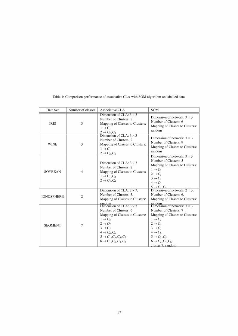
Table 1: Comparison performance of associative CLA with SOM algorithm on labelled data.

Data Set Number of classes Associative CLA SOM

IRIS 3

Dimension of CLA: 3×3Number of Clusters: 2Mapping of Classes to Clusters:1 →C12 →C2,C3

Dimension of network: 3×3Number of Clusters: 6Mapping of Classes to Clusters:random

WINE 3

Dimension of CLA: 3×3Number of Clusters: 2Mapping of Classes to Clusters:1 →C12 →C2,C3

Dimension of network: 3×3Number of Clusters: 9Mapping of Classes to Clusters:random

SOYBEAN 4

Dimension of CLA: 3×3Number of Clusters: 2Mapping of Classes to Clusters:1 →C1,C22 →C3,C4

Dimension of network: 3×3Number of Clusters: 5Mapping of Classes to Clusters:1 →C12 →C13 →C14 →C25 →C3,C4

IONOSPHERE 2

Dimension of CLA: 2×3,Number of Clusters: 3,Mapping of Classes to Clusters:random

Dimension of network: 2×3,Number of Clusters: 6,Mapping of Classes to Clusters:random

SEGMENT 7

Dimension of CLA: 3×3Number of Clusters: 6Mapping of Classes to Clusters:1 →C22 →C73 →C74 →C4,C65 →C1,C3,C5,C76 →C1,C3,C4,C5

Dimension of network: 3×3Number of Clusters: 7Mapping of Classes to Clusters:1 →C22 →C43 →C74 →C65 →C3,C56 →C2,C4,C6cluster 7: random

17

Noise Output Intra similarity Inter similarity

0.05

0.1

0.2

0.3

0.7

1

Figure 12: Effect of random noise on the output of the proposed clustering algorithm, intra similarity and inter similarity.

18

Learning Rate Output Intra similarity Inter similarity

0.05

0.1

0.3

0.5

0.7

1

Figure 13: Effect of learning rate on the output of the proposed clustering algorithm, intra similarity and inter similarity.

19

5.2 Image SegmentationIn order to evaluate the performance of the associative CLA in image segmentation, several standard images are prepared. Theseimages have been taken from Berkeley University repository for image segmentation [39]. In this experiment, associative CLAis applied on test data. Considering test data, dimension of CLA is selected as 4×4. This dimension is fixed for all images. So,each test image is segmented to 16 partitions at most. For better representation of the output, each segment is coloured differently.The proposed algorithm is iterated 30 times.

K-Means algorithm can be used in image segmentation, because image segmentation is as a clustering task on pixels ofthe image. K-Means algorithm for image segmentation is as follows: Same as in the proposed CLA, each pixel of the imageis represented as a 〈x,y,h,s,v〉. These five values are normalized and lie in [0,1] interval. Set of image’s pixels are given toK-Means algorithm and output of the algorithm is clusters of similar pixels. Number of clusters (K) must be determined beforeexecution of the algorithm and is given to it. Figure 14 shows result of applying associative CLA and K-Means on test images.

In figure 14, parameter K for K-Means algorithm is set from top to bottom as follows: 5, 8, 6, 4, 4, 4, and 7, respectively.If parameter K is set to more or less than real number of segments, that a person can detect in image, the result of the K-Meanswould not be acceptable. In all experiments, parameter K is set to the best value, so that the algorithm generate its best result. Inthe other side, K-Means has stochastic nature and generate different results on different runs. So, we reported the best of all.

Comparing the results of the proposed model with those of K-Means shows that the associative CLA performs better in almostall cases. Result of the CLA, unlike the K-Means, is such that structure of the image is conserved. Moreover, the proposed CLAis independent of the number of clusters and has a fixed structure in all experiments, while K-Means need to be given number ofclusters in each experiment.

5.3 Classification AlgorithmClassification is task of identifying to which of a set of categories a new observation belongs, on the basis of a training set ofdata. In order to evaluate performance of the proposed CLA in classification task, two experiments are designed. In the firstexperiment, associative CLA is applied on eight data sets. Result of the proposed CLA is compared with three famous andsuccessful classifiers: SVM, KNN and Naive Bayes classifier. In the next experiments, effect of parameters of the CLA on theperformance of classification is investigated.

5.3.1 Accuracy of the Proposed algorithm

In experiment one, eight data set are used which consist of IRIS, WINE, WDBC, PROTEIN, SOYBEAN, IONOSPHERE,DIABETES and SEGMENT. WDBC data set is extracted from digitized images of breast mass. This data set is used for diagnosisof breast cancer and has two classes of "Yes" or "No". PROTEIN data set is collected to study the structure of the proteinmolecules and has six classes. DIABETES data set is collected from many diabetics. This data set is used for separating diabetestype one from type two.

One of the powerful methods in classification is support vector machine (SVM). SVMs consider task of classification as anoptimization problem and solve it by quadratic programming. Kernel function, which is used in our experiment, is a polynomialfunction with order three. KNN is another efficient classification algorithm. KNN classifier finds k nearest neighbours of a testdata and puts it on the class which has the majority of votes among k neighbours. If k is set to a small or a large value, accuracy ofthe classifier decreased. Because small values prevent the voting to show the real class and large values allow the interference ofirrelevant data. So parameter k should be selected as a medium value, which of course depends on the data set. In this experiment,k is set to seven. Another classifier, which used for comparison, is Naive Bayes classifier. In the Bayesian framework, decisionfunction for class Ci is defined in equation (5).

gi(x) = P(Ci)×P(x|Ci), (5)

where, P(Ci) and P(x|Ci) show prior probability and liklihood of data given class Ci, respectively. For computing liklihooddistribution of class Ci over x should be known. Since these data sets are collected from natural events, distributions P(x|Ci) isregarded as normal distribution and parameters of this distribution, µ and Σ, are estimated from mean and variance of data set.So, probability of each test data is computed for each class of data set. Class which has the most probability is selected for testdata.

The proposed CLA is configured as follows: cells were arranged in n× 20 structure in two-dimensional Euclidean space,which n is number of classes of data set. In general, the number of columns is an experimental parameter and should bedetermined through trial and error. Later the effect of this parameter on the result of algorithm is studied. Neighbourhood vectoris set to N = {−5,−4,−3,−2,−1,0,1,2,3,4,5}. The number of iteration is set to 1000. For fair evaluation, 10-fold cross

20

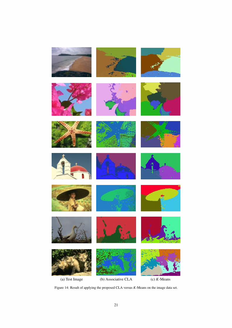
(a) Test Image (b) Associative CLA (c) K-Means

Figure 14: Result of applying the proposed CLA versus K-Means on the image data set.

21

Table 2: Comparison of the proposed classifier with SVM, KNN and Naive Bayes according to the CCR measure.

Data set Associative CLA SVM KNN Naive Bayes

IRIS 0.95 0.97 0.97 0.84WINE 0.81 0.95 0.69 0.67WDBC 0.91 0.95 0.93 0.83

PROTEIN 0.72 0.74 0.76 0.61SOYBEAN 0.94 0.97 0.95 0.88

IONOSPHERE 0.85 0.87 0.83 0.75DIABETES 0.72 0.76 0.73 0.68SEGMENT 0.87 0.88 0.88 0.76

average 0.84 0.88 0.84 0.75

(a) Learning Rate (b) Size of CLA (c) Noise

Figure 15: Effect of input parameters on proposed classification algorithm.

validation method is employed: each classification algorithm is repeated ten times. In each repetition, ten percent of the data setis used for the test and the remaining is used for the training. Correct classification rate (CCR) of classifier is computed in eachrepetition and the average of all CCRs is reported. Table 2 shows the results of four classifiers on the eight data sets.

The results in Table 2 show that the average CCR of the proposed classifier is better than Naive Bayes classifier and is similarto the KNN. SVM classifier is the best among four algorithms. Although, SVM results are better than associative CLA, thedifference is small and these algorithms have similar CCRs in most cases.

5.3.2 Sensitivity of the proposed algorithm to its parameters

In this and the next experiments, the effect of parameters on the performance of the proposed classifier is investigated. Parametersunder study include size of the CLA, learning rate and noise. First, the sensitivity of the proposed classification algorithm to thelearning rate is examined. This parameter appears in updating function of cells. Same as the previous experiment, dimension ofthe CLA is 3×20, neighbourhood radius is five, random noise is chosen uniformly in the interval [0,1], the number of iterationis set to 1000. Learning rate belongs to the interval [0,10] and 10-fold cross validation was employed on WINE data set. Figure15a represents the precision of classification versus different values of learning rate. Increasing learning rate from zero to three,rapidly increases accuracy of the algorithm and then does not change it. For values larger than three, precision of classificationdecreases. This results are expectable, because for small values of learning rate, change of cell’s state is slowly and negligible.For large values of learning rate, state of cell changes rapidly and could model the discriminant function. As a result, learningrate is an important parameter of the algorithm and should set to a value not too small and not too large.

In the next experiment, the effect of CLA’s size is studied. Size of CLA is another important parameter of the algorithm. Inthis experiment, dimension of CLA is 2× k, where k changes from 10 to 300. Random noise is chosen uniformly in the interval[0,1] and the learning rate is 0.5. Neighbourhood radius is set to five and the number of iterations is set to 1000. IONOSPHEREis used for evaluation and 10-fold cross validation is used for evaluation. As Figure 15b shows, increasing size parameter till 120causes increasing precision of the algorithm. After 120, precision decreases slowly. This result implies that the best value forsize is near 120 and small or large values for size lead to decreasing precision of the algorithm. This is because size of CLA is astructural parameter which determines the learning power of the classifier model. When the number of parameters for the model

22

Table 3: Comparison of the semi-supervised classifier based on the proposed CLA with semi-supervised SVM, KNN and Bayesian accordingto CCR measure, p = 0.3.

Data set Associative CLA SVM KNN Bayesian classifier

IRIS 0.92 0.98 0.96 0.90WINE 0.87 0.92 0.67 0.72WDBC 0.91 0.95 0.93 0.83

PROTEIN 0.71 0.73 0.78 0.69SOYBEAN 0.92 0.98 0.97 0.78


average 0.84 0.88 0.83 0.76

Table 4: Comparison of semi-supervised classifier based on the proposed CLA with semi-supervised SVM, KNN and Bayesian according toCCR measure, p = 0.5.


IRIS 0.90 0.97 0.96 0.88WINE 0.83 0.95 0.68 0.70WDBC 0.88 0.94 0.94 0.79

PROTEIN 0.69 0.72 0.64 0.63SOYBEAN 0.90 1 0.90 0.71


average 0.81 0.88 0.81 0.71

is small, that model cannot learn patterns in data well. Meanwhile, when a model is excessively complex, such as having toomany parameters, overfitting may occurs and so the prediction performance of the model decreases. As a result, size of CLA inthe proposed classification algorithm is an important parameter, which should be determined according to the nature of the data.

The last experiment of this section is devoted to effect of noise on the proposed classification algorithm. Data set for thisexperiment is IRIS. Dimension of CLA is set to 3×20 and the neighbourhood radius is five. Learning rate is set to 0.5 and thenumber of iterations is 1000. Value of the noise is chosen to be in the interval [0,10]. Method of validation is 10-fold crossvalidation. Figure 15c demonstrates the result. Value of η for the noise means that the random noise parameter, which is usedin AR−P, is chosen in the interval [−η,η] with uniform distribution. So, larger value for η causes the longer interval of randomnoise. Increasing noise from zero to two, does not change precision of the proposed algorithm significantly. However, for valueslarger than two, precision decreases until it reaches zero. This is because large values of random noise cause to cells select actionsrandomly and so their selection is not based on their previous learning. The primary idea of random noise is to give chance tocells to escape from local optimums. So the value of random noise should not be large to prevent from random walk of cells.

5.4 Semi-supervised Classification AlgorithmEvaluation of the associative CLA for semi-supervised classification problem is done on same data sets which are used forclassification problem. Semi-supervised methods used for comparison are SVM, KNN and Bayesian classifier. Associative CLAfor this problem configured so it has n×20 cells, with neighbourhood radius five. CLA algorithm is iterated 1000 times on eachdata set. To prepare data sets for semi-supervised classification, label of some percent of data is removed and the experiment isrepeated for different values. This value denoted by p, is written in caption each table. For ensuring reliability of the results, eachof four algorithms is repeated ten times and the average of ten results is reported as correct classification rate of that algorithm.

As tables 3, 4 and 5 show, as percent of unlabelled data increases, CCR of four algorithm decrease. This is because accuracyof training samples decreases and so error rate on test samples increases. Proposed CLA has average accuracy less than SVMalgorithm, greater than Bayesian classifier in all cases and better than KNN in some cases. To sum up, above tables show that,the associative CLA have an acceptable performance in semi-supervise classification task.

23

Table 5: Comparison of semi-supervised classifier based on the proposed CLA with semi-supervised SVM, KNN and Bayesian according toCCR measure, p = 0.8.


IRIS 0.84 0.87 0.95 0.72WINE 0.80 0.93 0.67 0.61WDBC 0.85 0.88 0.93 0.64

PROTEIN 0.59 0.56 0.61 0.58SOYBEAN 0.74 0.78 0.73 0.62


average 0.75 0.78 0.77 0.62

6 Conclusion and Future WorksIn this paper a new model for CLA was proposed. The main characteristic of this model is that it can receive additional infor-mation from the environment as the input vector. The external input is given to all cells of the CLA. Each cell uses the input inthe learning process. This augmentation increases flexibility and computational power of the CLA. Decision based on local in-formation, distribution of computation and stochastic nature of decisions are the main features of the associative CLA. Althougheach cell decides based on its local information, adding external input vector causes synchronization among cells.

Associative CLA can be utilized in pattern recognition applications. In this paper, some of these applications have beenintroduced and performance of the proposed algorithms has been investigated through several experiments on various data sets.Results of computer simulations show that the associative CLA outperforms successful algorithms in the studied applications. Inthe clustering and image segmentation tasks the results were compared intuitively. In the most of cases associative CLA beatsits rivals in detecting coherent clusters of the data and meaningful segments of the images. In the classification task, precisionof the proposed algorithm on eight data sets is 84% in average, which is better than KNN and Naive Bayes algorithms withprecision 83% and 75%, respectively. Meanwhile associative CLA acts worse than SVM with precision 88% . The similar resultis obtained when the proposed semi-supervised algorithm competes with semi-supervised SVM, KNN and Bayesian classifierson the same data sets. At all configurations, associative CLA outperforms Naive Bayes with significant difference; while itsperformance is close to semi-supervised KNN and is lower than semi-supervised SVM with narrow margin.

Experimental results on effect of the parameters of the algorithms demonstrated that the size of CLA is a structural parameter,which determines generalization power of the model. Random noise parameter, which used in choosing action function of LAs,helps the model to escape from local optimums and get the chance to reach the global optimum of the input space.

As the future work, we propose to design and implement some algorithms based of the associative CLA for the other tasks ofthe machine learning such as regression and dimension reduction. Comparing the resulting algorithms with the other successfulalgorithms of the pattern recognition such as artificial neural networks is suggested. Also, it would be beneficial to use theother learning algorithms, instead of the LA, inside each cell of the CLA to produce new learning models and compare theirperformance with the associative CLA .

AcknowledgementsThe authors would like to thank the anonymous reviewers for their valuable comments and suggestions which improved thepaper.

References[1] M. R. Meybodi, H. Beigy, and M. Taherkhani, “Cellular learning automata and its applications,” Sharif Journal of Science

and Technology, vol. 19, no. 25, pp. 54–77, 2003. pages 1

[2] M. Kharazmi and M. R. Meybodi, “Image segmentation using cellular learning automata,” in Proceeding of 10th IranianConf. on Electrical Engineering, ICEE-96, 2001. pages 1

24

[3] A. Abin, S. H. Amiri, and H. Beigy, “Cellular learning automata in image processing applications,” CSI Journal of ComputerScience and Engineering, vol. 8, pp. 37–52, 2010. pages 1, 3

[4] H. Beigy and M. R. Meybodi, “A self-organizing channel assignment algorithm: a cellular learning automata approach,”Springer- Verlag Lecture Notes in Computer Science, vol. 2690, pp. 119–126, 2003. pages 1, 3

[5] H. Beigy and M. R. Meybodi, “Cellular learning automata based dynamic channel assignment algorithms,” InternationalJournal of Computational Intelligence and Applications, vol. 8, no. 3, pp. 287–314, 2009. pages 1, 3

[6] M. R. Khojasteh and M. R. Meybodi, “Cooperation in multi-agent systems using learning automata,” Iranian Journal ofElectrical and Computer Engineering, vol. 1, pp. 81–91, 2004. pages 1

[7] M. Esnaashari and M. R. Meybodi, “Dynamic point coverage problem in wireless sensor networks: a cellular learningautomata approach.,” Adhoc & Sensor Wireless Networks, vol. 10, 2010. pages 1

[8] M. Esnaashari and M. Meybodi, “Deployment of a mobile wireless sensor network with k-coverage constraint: a cellularlearning automata approach,” Wireless networks, vol. 19, no. 5, pp. 945–968, 2013. pages 1

[9] R. Vafashoar, M. Meybodi, and A. M. Azandaryani, “CLA-DE: a hybrid model based on cellular learning automata fornumerical optimization,” Applied Intelligence, vol. 36, no. 3, pp. 735–748, 2012. pages 1

[10] B. Moradabadi and H. Beigy, “A new real-coded bayesian optimization algorithm based on a team of learning automata forcontinuous optimization,” Genetic Programming and Evolvable Machines, vol. 15, no. 2, pp. 169–193, 2014. pages 1

[11] M. Thathachar and P. S. Sastry, “Varieties of learning automata: an overview,” Systems, Man, and Cybernetics, Part B:Cybernetics, IEEE Transactions on, vol. 32, no. 6, pp. 711–722, 2002. pages 2

[12] G. Santharam, P. Sastry, and M. A. L. Thathachar, “Continuous action set learning automata for stochastic optimization,”Journal of the Franklin Institute, vol. 331, no. 5, pp. 607–628, 1994. pages 2

[13] H. Beigy and M. R. Meybodi, “A new continuous action-set learning automaton for function optimization,” Journal ofFrankline Institue, vol. 343, pp. 27–47, Jan. 2006. pages 2

[14] B. J. Oommen and E. V. de St Croix, “Graph partitioning using learning automata,” IEEE Transactions on Computers,vol. 45, pp. 195–208, Feb. 1996. pages 2

[15] H. Beigy and M. R. Meybodi, “Call admission control in cellular mobile networks: a learning automata approach,” inProceeding of EurAsia-ICT 2002: Information and Communication Technology, pp. 450–457, Springer, 2002. pages 2

[16] H. Beigy and M. R. Meybodi, “Learning automata based dynamic guard channel algorithms,” Computers & ElectricalEngineering, vol. 37, no. 4, pp. 601–613, 2011. pages 2

[17] M. Meybodi and H. Beigy, “Solving stochastic shortest path problem using distributed learning automata,” in Proceedingsof CSICC-2001, Isfehan, Iran, pp. 70–86, 2001. pages 2

[18] H. Beigy and M. R. Meybodi, “Utilizing distributed learning automata to solve stochastic shortest path problems,” In-ternational Journal of Uncertainty, Fuzziness and Knowledge-Based Systems, vol. 14, no. 5, pp. 591–615, 2006. pages2

[19] H. Beigy and M. R. Meybodi, “Adaptation of parameters of BP algorithm using learning automata,” in Proceedings of VIBrazilian Symposium on Neural Networks, SBRN2000, Brazil, pp. 24–31, Nov. 2000. pages 2

[20] M. R. Meybodi and H. Beigy, “Neural network engineering using learning automata: determining of desired size of threelayer feedforward neural networks,” Journal of Faculty of Engineering, vol. 34, pp. 1–26, Mar. 2001. pages 2

[21] H. Beigy and M. R. Meybodi, “A learning automata-based algorithm for determination of the number of hidden units forthree layer neural networks,” International Journal of Systems Science, vol. 40, pp. 101–118, Jan. 2009. pages 2

[22] B. Huberman, “Probabilistic cellular automata,” Nonlinear Phenomena in Physics, pp. 129–137, 1985. pages 3

[23] D. M. Forrester, Fuzzy cellular automata. PhD thesis, University of Ottawa, 2011. pages 3

25

[24] H. Beigy and M. R. Meybodi, “A mathematical framework for cellular learning automata,” Advances in Complex Systems,vol. 7, pp. 151–159, Feb. 2004. pages 3

[25] H. Beigy and M. R. Meybodi, “Asynchronous cellular learning automata,” Automatica, vol. 44, pp. 1350–1357, May 2008.pages 3

[26] H. Beigy and M. R. Meybodi, “Open synchronous cellular learning automata,” Advances in Complex Systems, vol. 10,no. 04, pp. 527–556, 2007. pages 3

[27] H. Beigy and M. R. Meybodi, “Cellular learning automata with multiple learning automata in each cell and its applications,”IEEE Transactions on Systems, Man, and Cybernetics, Part B: Cybernetics,, vol. 40, no. 1, pp. 54–65, 2010. pages 3

[28] J. Akbari Torkestani and M. R. Meybodi, “A cellular learning automata-based algorithm for solving the vertex coloringproblem,” Expert Systems with Applications, vol. 38, no. 8, pp. 9237–9247, 2011. pages 3

[29] R. Ghaderi, M. Esnaashari, and M. R. Meybodi, “An adaptive scheduling algorithm for set cover problem in wireless sensornetworks: a cellular learning automata approach,” International Journal of Machine Learning and Computing, vol. 2,pp. 626–632, 2012. pages 3

[30] M. Esnaashari and M. R. Meybodi, “A cellular learning automata-based deployment strategy for mobile wireless sensornetworks,” Journal of Parallel and Distributed Computing, vol. 71, no. 7, pp. 988–1001, 2011. pages 3

[31] S. Shafeie and M. Meybodi, “A self-organized energy efficient topology control protocol based on cellular learning automatain wireless sensor networks (seetcla),” in Proceeding of 4th International Congress on Ultra Modern Telecommunicationsand Control Systems and Workshops, pp. 974–980, 2012. pages 3

[32] H. Beigy and M. R. Meybodi, “An adaptive call admission algorithm for cellular networks,” Computers & ElectricalEngineering, vol. 31, no. 2, pp. 132–151, 2005. pages 3

[33] A. G. Barto and P. Anandan, “Pattern-recognizing stochastic learning automata,” IEEE Transactions on Systems, Man andCybernetics, no. 3, pp. 360–375, 1985. pages 4, 7

[34] M. A. L. Thathachar and V. V. Phansalkar, “Learning the global maximum with parameterized learning automata,” IEEETransactions on Neural Networks, vol. 6, pp. 398–406, may 1995. pages 4

[35] T. G. Dietterich and G. Bakiri, “Solving multiclass learning problems via error-correcting output codes,” Journal of artificialintelligence research, pp. 263–286, 1995. pages 7

[36] X. Wu, V. Kumar, J. R. Quinlan, J. Ghosh, Q. Yang, H. Motoda, G. J. McLachlan, A. Ng, B. Liu, S. Y. Philip, Z.-Z. Zhou,M. Steinbach, D. J. Hand, and D. Steinberg, “Top 10 algorithms in data mining,” Knowledge and Information Systems,vol. 14, no. 1, pp. 1–37, 2008. pages 10

[37] Burkardt Clustering dataset, “http://people.sc.fsu.edu/ burkardt/datasets/cvt,” Accessed in April 2014, 2014. pages 11

[38] UCI Machine Learning Repository, “http://archive.ics.uci.edu/ml/,” Accessed in April 2014, 2014. pages 14

[39] Segmentation Dataset, “http://www.eecs.berkeley.edu/research/projects/cs/vision/grouping/segbench,” Accessed in April2014, 2014. pages 20

26

associative cellular learning automata and its applicationssharif.edu/~beigy/docs/2017/atb17.pdf ·...

Documents