boundary-integ al methods in elasticity and plasticity … · bqundary-integ~l methods in...

* -

a NASA TN 0-7418

h n

BOUNDARY-INTEG AL METHODS IN ELASTICITY AND PLASTICITY

by Alexdnder M endelson

Lewis Resedrch Center Clevehnd, Ohio 44135

N A T I O N A L A E R O N A U T I C S A N D SPACE A D M I N I S T R A T I O N e W A S ~ I N G T O N , D. C. e NOVEMBER 1973

https://ntrs.nasa.gov/search.jsp?R=19740002724 2018-07-19T04:58:50+00:00Z

1. Report No.

NASA TN D-7418 2. Government Accession No. 3. Recipient’s Catalog No.

4. Title and Subtitle BOUNDARY-INTEGRAL METHODS IN ELASTICITY AND PLASTICITY

* For sale by the National Technical Information Service, Springfield, Virginia 22151

5. Report Date November 1973

6. Performing Organization Code

7. Author(s)

Alexander Mendelson

9. Performing Organization Name and qddress

Lewis Research Center National Aeronautics and Space Administration Cleveland, Ohio 44135

12. Sponsoring Agency Name and Address

National Aeronautics and Space Administration Washington, D. C. 20546

.

8. Performing Organization Report No. E-7478

10. Work Unit No.

501-21 11. Contract or Grant No.

13. Type of Report and Period Covered

Technical Note 14. Sponsoring Agency Code

17. Key Words (Suggested by Author(s))

Elasticity Plasticity Solid mechanics Boundary integrals

18. Distribution Statement Unclassified - unlimited

Unclassified Domestic, $3.00 Foreign, $5.50 Unclassified 37

BQUNDARY-INTEG~L METHODS IN ELASTICITY AND PLASTICITY

by Alexander Mendelson

Lewis Research Center

SUMMARY

Recently developed methods that use boundary -integral equations applied to elastic and elastoplastic boundary value problems are reviewed. Direct, indirect, and semidirect methods using potential functions, stress functions, and displacement functions are described. Examples of the use of these methods for torsion problems, plane problems, and three-dimensional problems are given. It is concluded that the boundary- integral methods represent a powerful tool for the solution of elastic and elastoplastic problems.

INTRODUCTION

Methods of analysis in solid mechanics, as in most other scientific and engineering fields, have been revolutionized by the advent of the modern digital computer. Thus, purely numerical methods , such as finite differences, and analytical methods, whose final stages require numerical procedures such as complex variable methods, awaited the modern computer for their practical implementation to all but the simplest problems.

Although many general methods have been and are being used for solving problems in elasticity and plasticity, the currently most popular ones probably are (1) finite differences, (2) finite elements, and (3) complex variables. To this list we may now add the boundary -integral methods. It is the boundary -integral methods that are discussed in this report.

First, the question might be asked, why is it necessary to get involved in yet another method for solving the same types of problems? What advantages do these methods have over the commonly used methods previously listed? The apparent advantages are as follows.

(1) The need for conformal mapping is obviated. (2) Uniform or mixed boundary value problems are handled with equal ease.

(3) Stresses and displacements a re obtained directly without need for numerical

(4) No special treatment is needed for multiply connected regions. (5) The internal stresses and displacements a re obtained only where and when

(6) The method can be extended directly to three -dimensional problems. (7) Nodal points are needed only on the boundary instead of throughout the interior

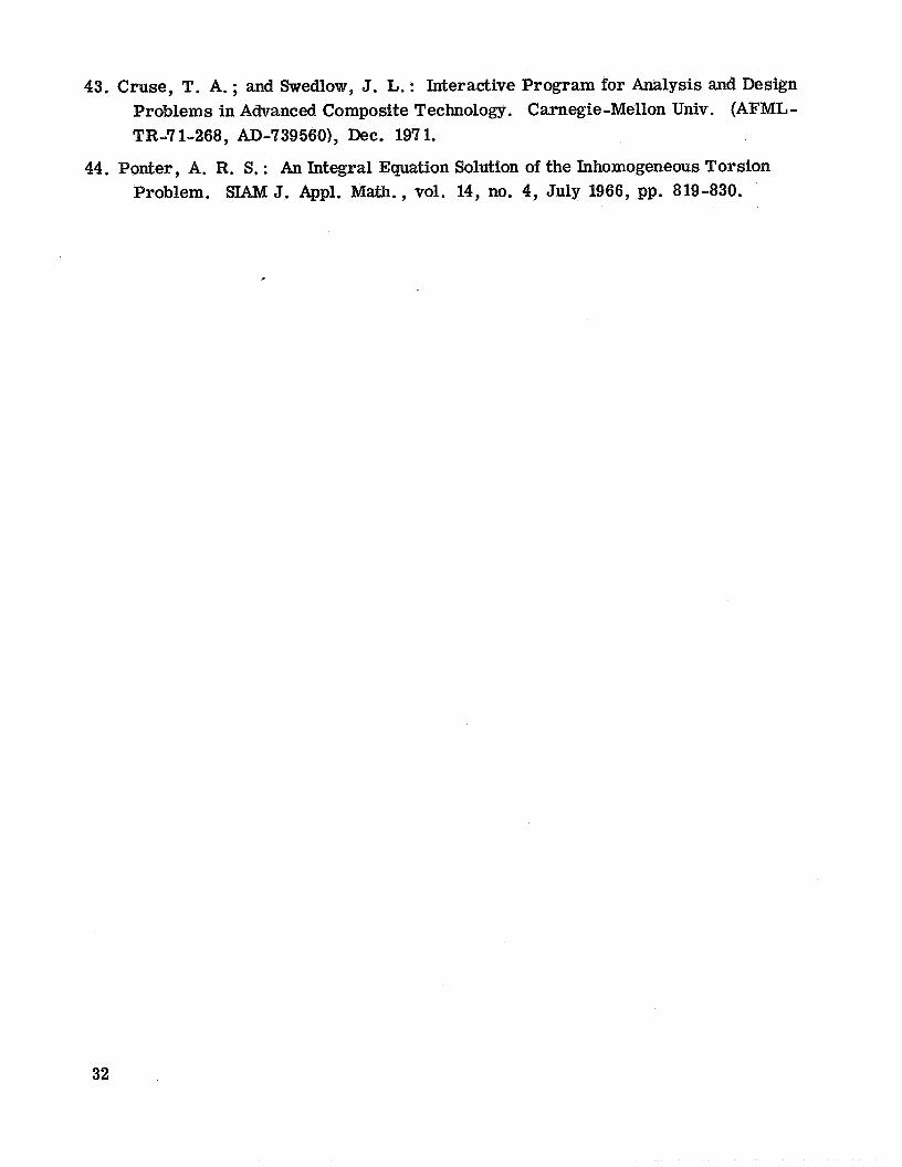
The last point, which is probably the most important one, is illustrated in figure 1.

differentiation.

needed.

(as required by finite-difference or finite-element methods).

For the finite-difference or finite-element methods, the whole region must be covered by a grid, producing a large number of nodal points and corresponding unknowns. Thus a large number of simultaneous equations must be solved. In the present methods, as will shortly be seen, nodal points a r e taken only on the boundary, resulting in a much smaller number of unknowns, the dimensions of the problem being effectively reduced by one.

On the other hand, the resulting matrices a re full, whereas in the finite-element methods, for example, the matrices are usually sparse and can be more or less banded.

The boundary integral methods themselves can be classified into three groups: indirect, semidirect, and direct.

The indirect methods formulate the problem in terms of unknown density functions, which have no physical significance. But once these density functions are determined, the displacements and/or stresses can be directly computed.

The semidirect methods formulate the problem in terms of unknown functions that are more familiar, such as the various stress functions. The stresses are then determined by simple differentiation.

The direct methods formulate the problem in terms of the direct physical quantities such as the displacements.

All three methods a re illustrated in the next section by application to the Saint- Venant torsion problem. Also shown is how the solution can be extended to elastoplastic torsion. The more complicated plane strain and plane stress problems are then considered. We conclude with a brief discussion of three -dimensional problems.

ematical one. Such questions a s the existence and uniqueness of solutions, the differences between internal and external problems, problems of convergence, etc. a r e not discussed. Excellent discussions of many of these questions can be found in references 1 to 6.

The subject is approached herein from the applied viewpoint and not from the math-

TORSION PROBLEM

The torsion problem can be formulated in many ways (refs. 7 and 8):

2

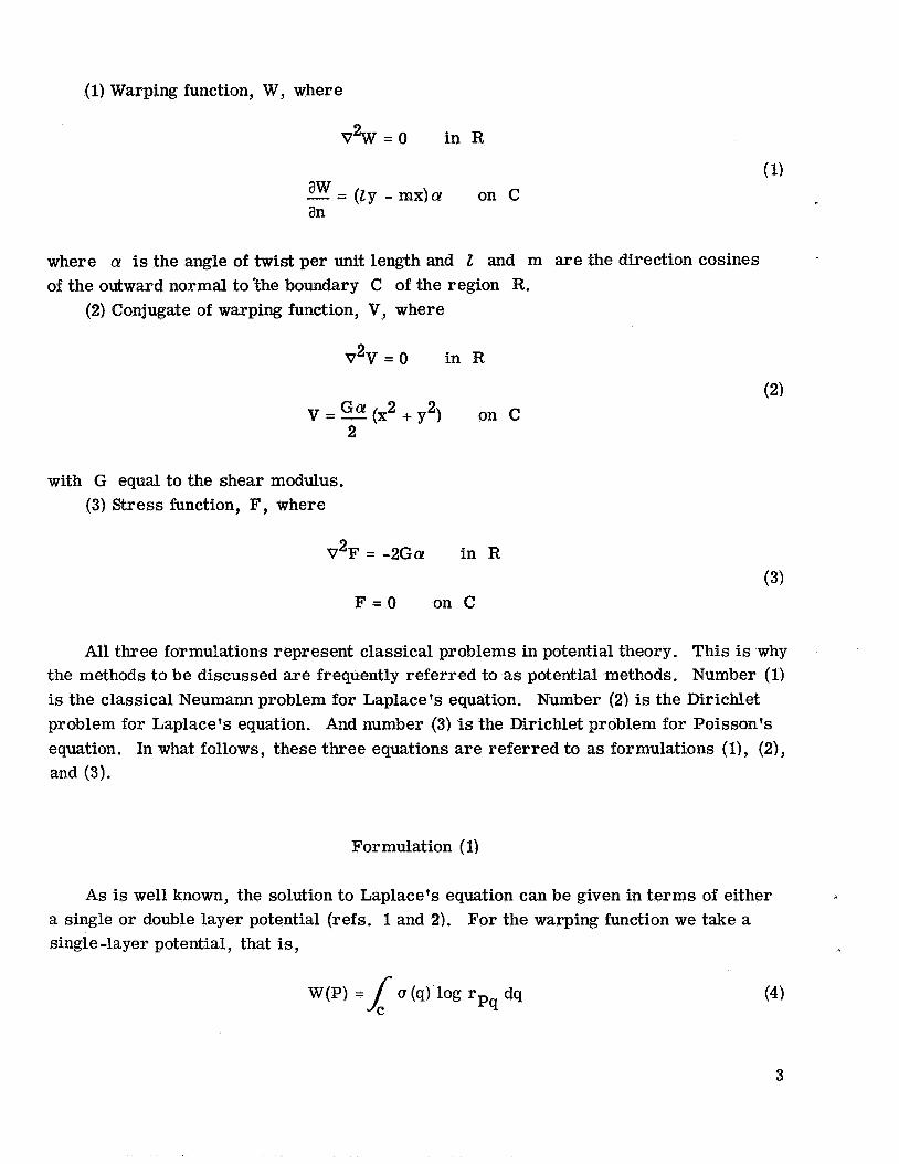
(1) Warping function, W, where

V % = O in R

- - aw - ( ~ y - mx)a! on c an

where a! is the angle of twist per unit length and I and m are the cirection cos of the outward normal tothe boundary C of the region R.

(2) Conjugate of warping function, V, where

2 V V = O in R

.ne s

2

with G equal to the shear modulus. (3) Stress function, F, where

2 V F = -2Ga! in R

F = O o n C

All three formulations represent classical problems in potential theory. This is why the methods to be discussed are frequently referred to as potential methods. Number (1) is the classical Neumann problem for Laplace's equation. Number (2) is the Dirichlet problem for Laplace's equation. And number (3) is the Dirichlet problem for Poisson's equation. In what follows, these three equations a re referred to as formulations (11, (Z), and (3).

Formulation (1)

As is well known, the solution to Laplace's equation can be given in terms of either a single or double layer potential (refs. 1 and 2). For the warping function we take a single -layer potential, that is,

3

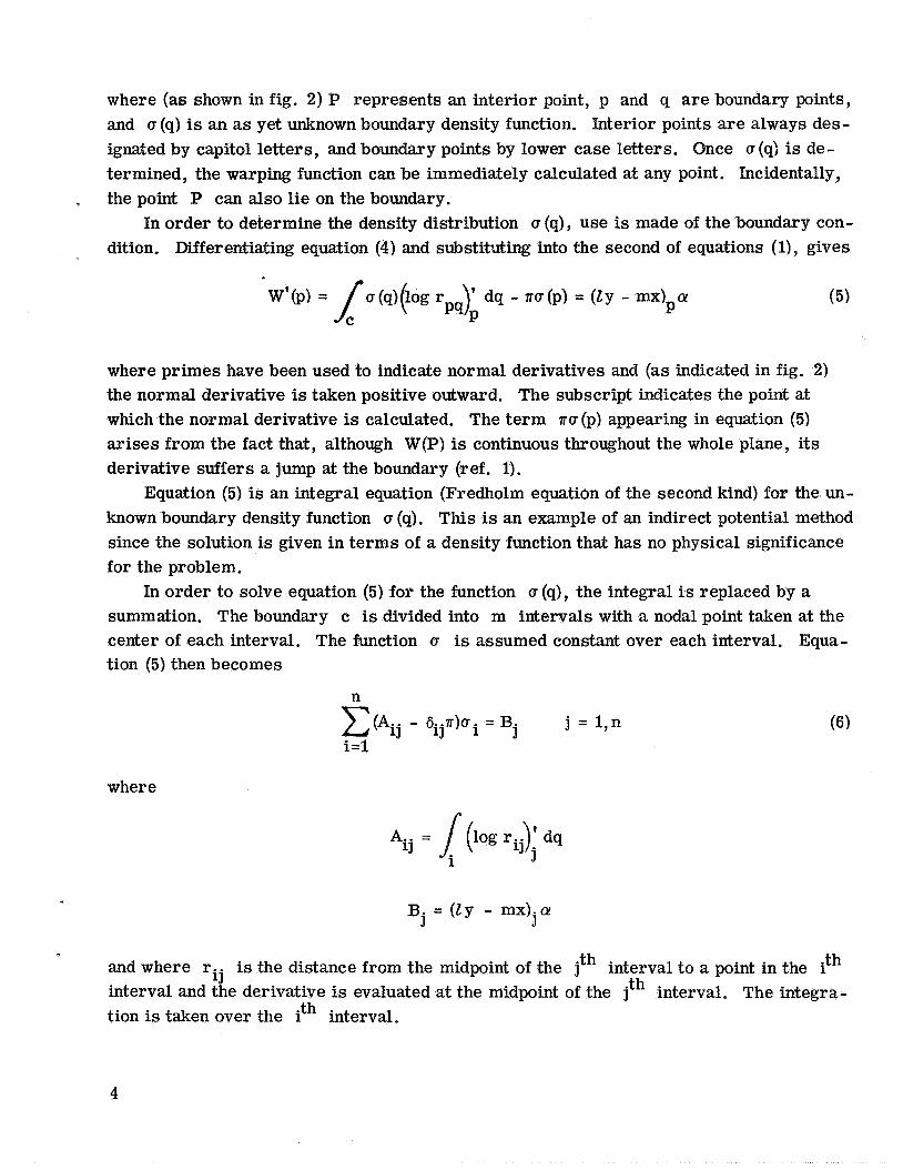
where (as shown in fig. 2) P represents an interior point, p and q a re boundary points, and u (q) is an as yet unknown boundary density function. Interior points a re always designated by capitol letters, and boundary points by lower case letters. Once u (q) is determined, the warping function can be immediately calculated at any point. Incidentally,

, the point P can also lie on the boundary. In order to determine the density distribution u (q), use is made of the boundary con-

dition. Differentiating equation (4) and substituting into the second of equations (1), gives

W'b ) = l u (q)(log rpq); dq - ru (p) = (l y - mx) P a! (5)

where primes have been used to indicate normal derivatives and (as indicated in fig. 2) the normal derivative is taken positive outward. The subscript indicates the point at which the normal derivative is calculated. The term nu(p) appearing in equation (5) arises from the fact that, although W(P) is continuous throughout the whole plane, its derivative suffers a jump at the boundary (ref. 1).

Equation (5) is an integral equation (Fredholm equation of the second kind) for the unknown boundary density function u (9). This is an example of an indirect potential method since the solution is given in terms of a density function that has no physical significance for the problem.

summation. The boundary c is divided into m intervals with a nodal point taken at the center of each interval. The function u is assumed constant over each interval. Equa- tion (5) then becomes

In order to solve equation (5) for the function ~ ( q ) , the integral is replaced by a

where

n (A.. - 6..n)oi = Bj j = l , n 13 1J

i= 1

B. = (Zy - mx).a! J J

th and where r.. is the distance from the midpoint of the jth interval to a point in the i interval and the derivative is evaluated at the midpoint of the jth interval. The integration is taken over the ith interval.

1.7

4

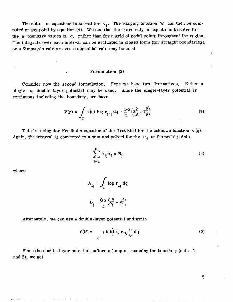
The set of n equations is solved for ai. The warping function W can then be computed at any point by equation (4). We see that there are only n equations to solve for the n boundary values of 0, rather than for a grid of nodal points throughout the region. The integrals over each interval can be evaluated in closed form (for straight boundaries), or a Simpson's rule or even trapezoidal rule may be used.

Formulation (2)

Consider now the second formulation. Here we have two alternatives. Either a single- or double-layer potential may be used. continuous including the boundary, we have

Since the single-layer potential is

This is a singular Fredholm equation of the first kind for the unknown function a (4). Again, the integral is converted to a sum and solved for the a i at the nodal points.

n E A i j a i = Bj

i= 1

where

Alternately, we can use a double -layer potential and write

Since the double-layer potential suffers a jump on reaching the boundary (refs. 1 and 2), we get

5

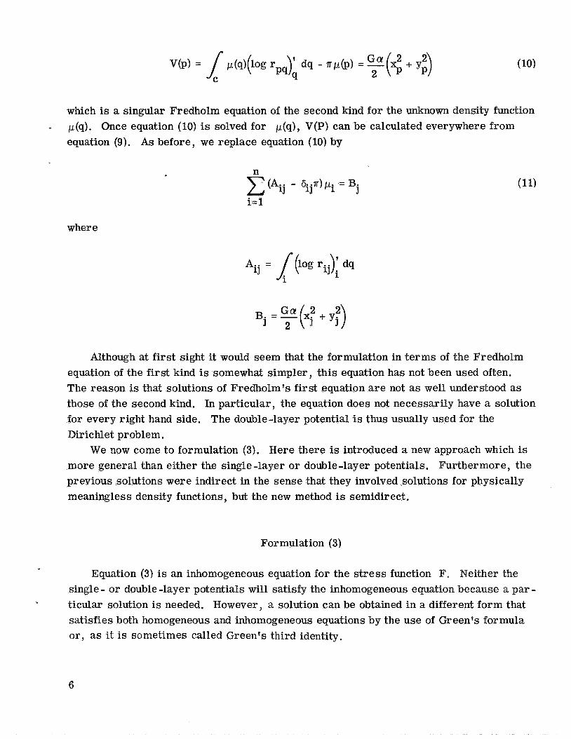
which is a singular Fredholm equation of the second kind for the unknown density function

equation (9). As before, we replace equation (10) by . p(q). Once equation (10) is solved for p(q), V(P) can be calculated everywhere from

n

i= 1

(Aij - Gijr)pi = B. 3

where

Although at first sight it would seem that the formulation in terms of the Fredholm equation of the first kind is somewhat simpler, this equation has not been used often. The reason is that solutions of Fredholm's first equation are not as well understood as those of the second kind. In particular, the equation does not necessarily have a solution for every right hand side. The double-layer potential is thus usually used for the Dirichlet problem.

We now come to formulation (3). Here there is introduced a new approach which is more general than either the single-layer or double-layer potentials. Furthermore, the previous solutions were indirect in the sense that they involved solutions for physically meaningless density functions, but the new method is semidirect.

Formulation (3)

Equation (3) is an inhomogeneous equation for the stress function F. Neither the single - or double -layer potentials will satisfy the inhomogeneous equation because a par - ticular solution is needed. However, a solution can be obtained in a different form that satisfies both homogeneous and inhomogeneous equations by the use of Green's formula or, as it is sometimes called Green's third identity.

6

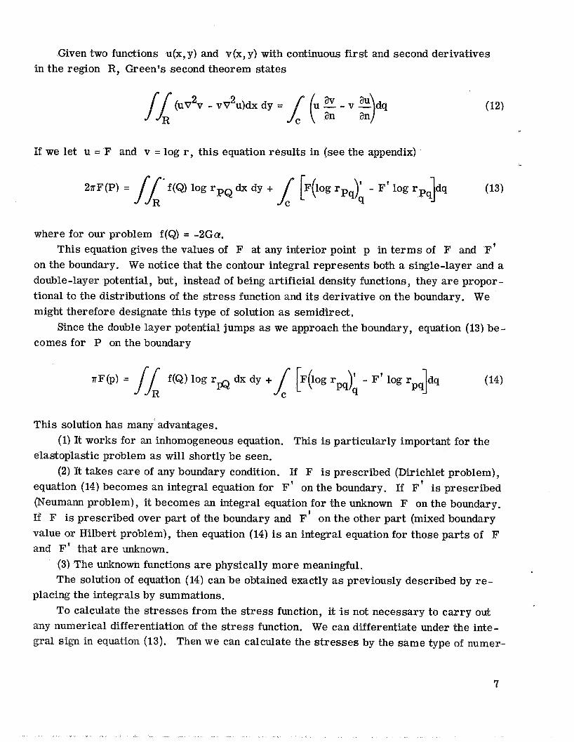
Given two functions u(x,y) and v(x,y) with continuous first and second derivatives in the region R, Green's second theorem states

2 2 (uV v - VV u)dx dy =

If we let u = F and v = log r, this equation results in (see the appendix)

where for our problem f(Q) = -2Ga.

on the boundary. We notice that the contour integral represents both a single-layer and a double-layer potential, but, instead of being artificial density functions, they are propor - tional to the distributions of the stress function and its derivative on the boundary. We might therefore designate this type of solution as semidirect.

comes for P on the boundary

This equation gives the values of F at any interior point p in terms of F and F'

Since the double layer potential jumps as we approach the boundary, equation (13) be-

This solution has many advantages. (1) It works for an inhomogeneous equation. This is particularly important for the

elastoplastic problem as will shortly be seen. (2) It takes care of any boundary condition. If F is prescribed (Dirichlet problem),

equation (14) becomes an integral equation for F' on the boundary. If F' is prescribed (Neumann problem), it becomes an integral equation for the unknown F on the boundary. If F is prescribed over part of the boundary and F' on the other part (mixed boundary value or Hilbert problem), then equation (14) is an integral equation for those parts of F and F' that are unknown.

(3) The unknown functions are physically more meaningful. The solution of equation (14) can be obtained exactly as previously described by re-

To calculate the stresses from the stress function, it is not necessary to carry out placing the integrals by summations.

any numerical differentiation of the stress function. We can differentiate under the integral sign in equation (13). Then we can calculate the stresses by the same type of numer-

7

ical integration as before, once F and F' are known on the boundary. This is a more accurate way of computing the stresses.

The use of Green's formula is of course not restricted to formulation (3) for the stress function. It can just as well be used for determining W or V, We just replace F by W in equations (13) and (14) and set f equal to zero. This solution is then referred to as a direct potential method, since we solve directly for the physical quantity desired, the warping function.

Some Numerical Results

A number of torsion problems have been solved by Jaswon and Ponter (ref. 9), including prismatic bars with cross sections consisting of solid and hollow ellipses, rec - tangles, equilateral triangles, and circles with curved notches. The direct potential method was used to determine the warping function. A few of the results taken from this reference are shown in table I. Results obtained by the present author for the square cross section using the stress function rather than the warping function were essentially the same. Excellent agreement is obtained with the known analytical results.

Elastoplastic Torsion

By use of Green's boundary formula we can treat the elastoplastic problem the same way as the elastic problem. With plastic flow occurring, the equation for the stress function can be written as

The function f in the double integral of Green's formula (eq. ( 4)) now contains the plastic flow terms indicated. ticity theory. The solution is an iterative one.

We start by assuming the plastic strains to be zero. The problem is then solved using Green's formula as indicated previously, and the stresses a re computed by differen-

hese terms are computed by the use of e usual plas-

then computes the total strains from the relations

8

and

and the equivalent total strains from

From the stress-strain curve of the material the equivalent, plastic strain is then obtained :

And the plastic strains are then given by

and

First approximations

p -‘P ‘ZX - - €ZX

‘et

p / P

‘et ZY

E - - € ZY

to the plastic strains and consequently for the function f(x,y) appearing in equation (15) have thus been determined. The process is then repeated until convergence is obtained. A more detailed discussion of the successive approximation method (or the “method of initial strains, as it is sometimes called) can be found in reference 10. Note that only the area integral, which represents the right hand side of the set of equations to be solved, changes from iteration to iteration. Note also that, although total plastic strains have been used in the previous equations for ease of writing, incremental strains could have been used just as well.

of a circular shaft for which the solution can be obtained in closed form if linear strainhardening of the material is assumed.

To illustrate the correctness of this type of formulation we can consider the problem

9

Consider a circular shaft of radius a. The radial coordinate will be designated by p, to distinguish it from r , the distance between the fixed point and the variable point appearing in the previous formulas. In polar coordinates, because of symmetry, the function f appearing in equation (15) becomes

For linear strain hardening, it follows that (ref. 10, p. 255)

=Ap + B Z 0

where

-43 (1 + V)EO B =

m (1 - m)

3 + 2(1 + v)

where v is Poisson's ratio, m is the strain hardening parameter (ratio of the slope of the strain hardening line to the elastic modulus), and

Green's boundary formula (eq. (14)) then becomes

is the yield strain. On the boundary F(a) = 0 and, because of axial symmetry, F'(a) = a constant.

B

P (2A - a! + - log r dx dy - F'(a)

PQ 0 = 2G

which, upon solving for F'(a), gives

Hence, for any interior point

28F(p) = 2 6 dx dy - F'(a)

10

or

F(p) = G - [(2A - cy)(p2 - a 2 ) + 4B(p - 2

and the shear stress r is given by

.=-"=2G[(%-.)p-B] aP

which agrees with the solution obtained in an entirely different fashion in reference 10. Note that this solution is valid only in the plastic region, that is, for p 2 pc where pc, the elastic-plastic boundary, is given by (ref. lo),

For p 5 pc the usual elastic solution prevails.

THEPLANEPROBLEM

We now consider the plane problem of elastoplasticity, that is, plane strain o r plane stress. The problem can be formulated in several ways: (1) by the use of the Airy stress function, which is a semidirect formulation, (2) by the use of singular solutions of the Navier equations, which is a direct formulation, or (3) by the use of fictitious loads, which is an indirect formulation. The second approach lends itself directly to the three- dimensional extension. The last method cannot easily take into account plastic flow.

Formulation in Terms of Airy Stress Function

In terms of the Airy stress function, we have to solve the problem (for plane stress),

4 V F =f(x,y) in R

where F and aF/an are given on the boundary, and

11

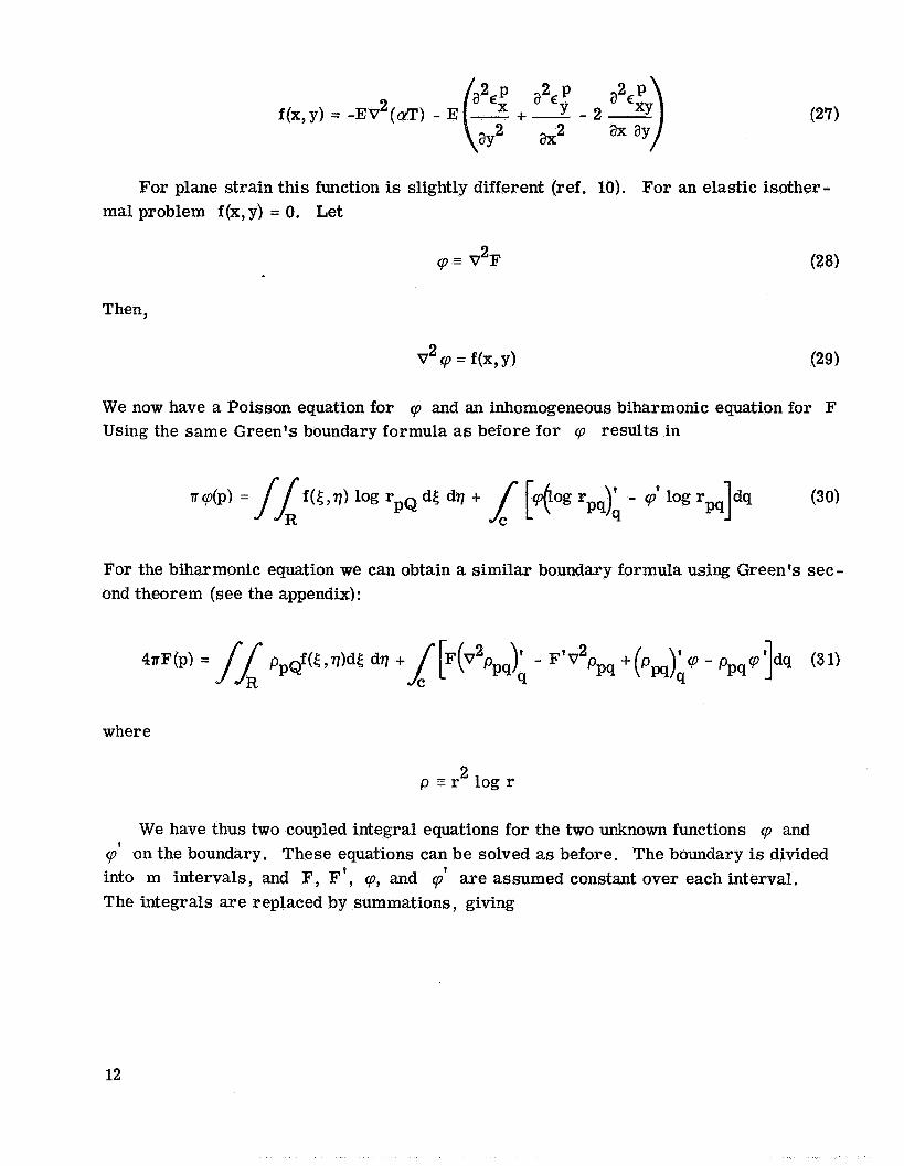
mal For plane strain this function is slightly different (ref. 10). For an elastic isother- problem f(x,y) = 0. Let

p= V2F (28)

Then,

(29) 2 v q = f ( x , y )

We now have a Poisson equation for 4p and an inhomogeneous biharmonic equation for F Using the same Green's boundary formula as before for q results in

For the biharmonic equation we can obtain a similar boundary formula using Green's second theorem (see the appendix):

where

2 p = r log r

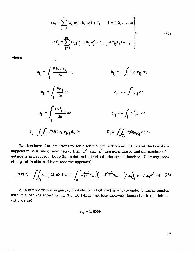
We have thus two coupled integral equations for the two unknown functions q and 50' on the boundary. These equations can be solved as before. The boundary is divided into m intervals, and F, F', 40, and cp) are assumed constant over each interval. The integrals are replaced by summations, giving

12

where

(a-p +b..$) +Ji i = 1 , 2 ,..., m m

"Vi = 1J J 11 J

(C-.y. + d..$ + e..F. + f..F!) + Ki lJ J 1J J 1J J 13 3

j = l

a log r.. a.. = lJ dq

1 J an J b-. 9 = - i l o g r.. 9 dq

d.. = - f pij dq 3 9

f.. 1J = - V2pij dq

We thus have 2m equations to solve for the 2m unknowns. If part of the boundary happens to be a line of symmetry, then F' and qt are zero there, and the number of unknowns is reduced. Once this solution is obtained, the stress function F at any inte- r ior point is obtained from (see the appendix)

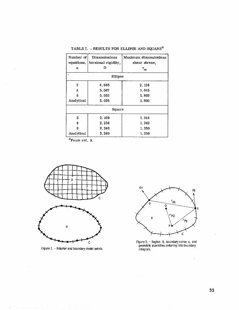
A s a simple trivial example, consider an elastic square plate under uniform tension with unit load (as shown in fig. 3). By taking just four intervals (each side is one interval), we get

ox = 1.0000

13

We now consider a problem that is by no means trivial, namely, the elastic thermal stress in a square plate under a parabolic temperature distribution. The solution has been obtained in various ways, the most accurate probably being a finite difference solution using a 20 by 20 grid and thus involving the solution of 400 simultaneous equations. A comparison of that result (ref. 11) with the present method using 60 intervals on the boundary is shown in figure 4. Actually, because of double symmetry, there a re only 15 equations to solve. As shown by the figure, good agreement w a s obtained.

A similar formulation has been used for plate bending problems in reference 12. Let us now consider a problem for which no good solution has been available here-

tofore, namely, the elastoplastic problem of an edge-notched beam under pure bending (fig. 5).

with T = 0. An iterative solution is performed as for the torsion problem except that the plane stress or plane strain plasticity equations a re used (ref. 10).

strain case. A complete discussion of this problem is presented in references 13 and 14.

The function f(x,y) appearing in equation (31) is the right hand side of equation (27)

Figure 5 shows the spread of the plastic zone with increasing load for the plane

Formulation in Terms of Potential Functions

The preceding problems can also be formulated in terms of single-layer density functions as for the torsion problem. This approach has been investigated in some detail in references 3 to 5 and 15 to 17. This formulation is based on the fact that a biharmonic function can always be represented in terms of two harmonic functions as shown in stand- ard elasticity books. Thus,

(34)

where Q! and /3 are harmonic functions and can therefore be represented in terms of single- o r double-layer potentials and rp is the distance from the point P to the or- igin of coordinates. We can thus write

(3 5)

and substituting into equation (34) on the boundary gives

64

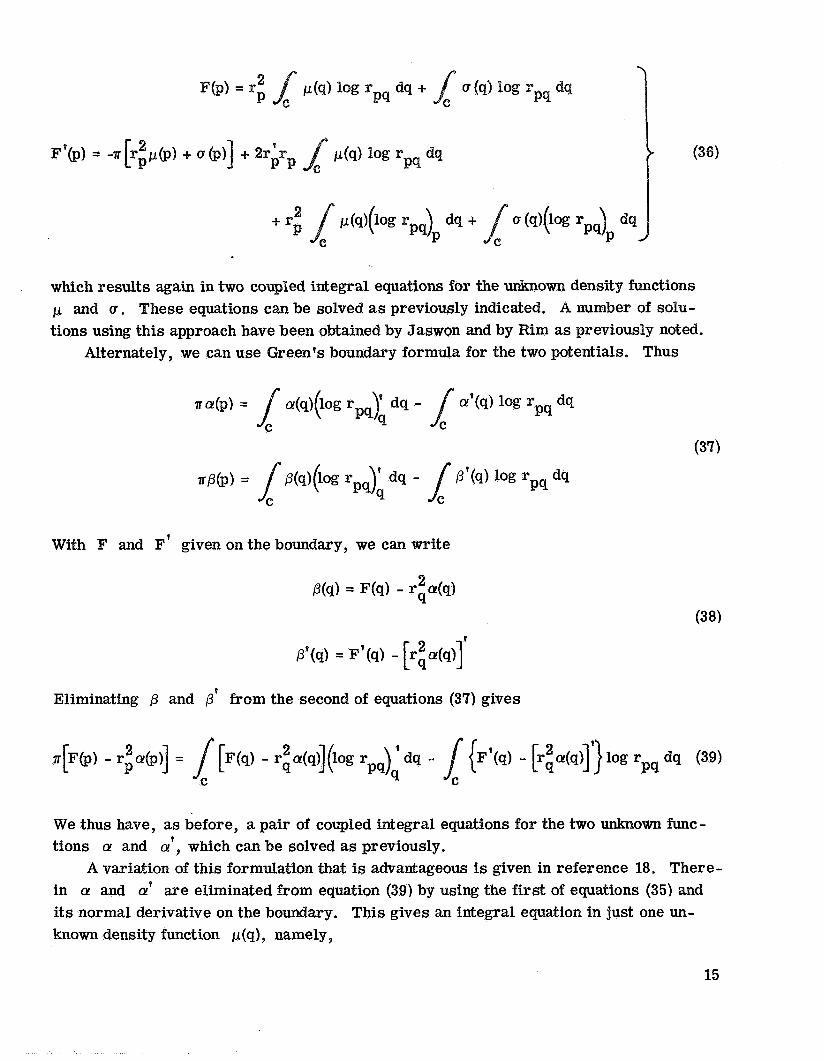
F(p) = r

which results again in two coupled integral equations for the unknown density functions p and a . These equations can be solved as previously indicated. A number of solutions using this approach have been obtained by Jaswon and by Rim as previously noted,

Alternately, we can use Green's boundary formula for the two potentials. Thus

With F and F' given on the boundary, we can write

P(q) = F(q) - r$q)

Eliminating P and (3' from the second of equations (37) gives

We thus have, as before, a pair of coupled integral equations for the two unknown functions a! and a!', which can be solved as previously.

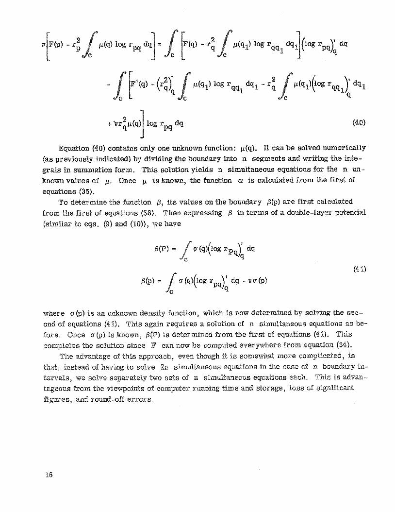
in a! and a!' are eliminated from equation (39) by using the f i r s t of equations (35) and its normal derivative on the boundary. This gives an integral equation in just one unknown density function p(q), namely,

A variation of this formulation that is advantageous is given in reference 18. There-

15

here

is a nd where

4 r

is a ion only of the geometry. ain, the integrals can ation was presented by Liu and coworkers (refs. 20 to 221,

e note that the method ho also considered multiply connected regions, bodies with axial symmetry, and ex-

rmulation to three-dimensional problems as well. y applicable to bodies wit isplacement boundary conditions. A similar ach has also been used b iveira (ref. 23) using complex potenti

e now come to a direct formu ation of the two-dimensional problem which is endable to three -dimensional problems. This formulation is on of the Navier equations.

he Navier equations for plane strain, including astic flow, temperat Y

a

and

enceforth the usual ensor notation e a repeated subsc summation over its range and a comma indicates partial differentiation. E?. represents the sum of all the plastic strain increments up to and incl

oissonPs ratio, Q! is the coefficient of line 13

8

here

at must be satisfied by the displacements over that the a re specified a re

for plane strain and

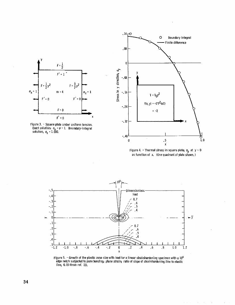
for plane stress. e now note the following interesting fact: y defining a pseud

seudoboundary force

n. + 3

we may write equations (45) and (46) for plane

- u. + e,i - - 2 1

(uiYj + u. 3 9 i )n. 3 + , kni

9

e

2 1

(55)

As previously noted all derivatives are taken at the variable point of integration. For the elastic problem all the plastic flow terms disappear.

for example, in references 6 and 26 to 30. These include problems of circular and ellip- t ic regions, rings, rectangles, bodies with holes, inclusions, notches, and cracks as well as some thermoelastic problems.

The Navier equations (45) and (46) and the corresponding solution (52) have been written in terms of displacements, stresses, and plastic strains. This is the appropriate form if the method of successive elastic solutions, or method of initial strains (ref. IO), is used to solve the elastoplastic problem. If the tangent modulus method is used (refs. 31 to 33), these equations a re written in terms of velocities, stress rates, and plastic strain rates. The boundary-integral formulation remains the same.

Solution to a number of elastic problems using these equations have been obtained,

THREE -DIMENSIONAL PROBLEMS

For three-dimensional problems the extension is direct. The Navier equations (45) retain the same form, except that the range of subscripts is now three and the Laplacian appearing in these equations is the three -dimensional Laplacian. The singular solution, instead of having a logarithmic singularity, has a l/r singularity. The solution then takes the same form as before, except that the kernels of the integrals are slightly different. The area integral becomes a volume integral, and the line integrals become surface integrals over the bounding surface of the body. Thus equation (52) becomes

where

22

1 [(3 - 4v)tjij + r,ir, 1 1 u.. + l3 16a(l - v)G r 1

Instead of dividing the boundary into a set of linear intervals, we now have to divide the bounding surface into a series of surface elements. These may be rectangular or triangular in shape a s in the two-dimensional finite-element formulation. The unknown functions are assumed constant over each element, and the integrals are replaced by sums over all the elements. If the surface is divided into m elements, we get 3m simultaneous equations to solve.

The stresses a re given by

a re as given by equations (55) and (57). The general elasto- where Vijk) Tijk, TijkZ plastic flow theory leading to these equations is given in reference 34.

Using this approach solutions have been obtained for several elastic problems in ref - erences 27 and 35 to 37 among others. Figures 7 and 8 show two such problems. Fig- ure 7 (from ref. 35) shows the results for the simple problem of a cube loaded in tension at one end, while on the other end, as well as on two normal faces, the normal displacement components a re set equal to zero. The results are shown for 12 surface elements, each surface being divided into two triangles. Good agreement is obtained with the exact solution.

An example of a much more difficult problem involving a semielliptical surface flaw in a plate subjected to tension is shown in figure 8 (from ref. 37). An exact solution is not available here for comparison. A similar problem is treated in reference 30.

CONCLUDING REMARKS

This brief survey indicates the potential of the boundary integral methods for solving two- and three-dimensional elastic and elastoplastic problems. The more important advantages of these methods are the reduction of the problem size, since the unknown quantities appear only on the boundaries, and the ability to handle arbitrarily shaped

23

boundaries. This advantage is particularly apparent in using the direct -method involving the Navier equations, since neither smooth boundaries nor simply connected regions a re required.

isotropic materials. References 38 to 40 formulate the general transient elastodynamic problem. Reference 4 1 discusses the linear viscoelastic problem; references 42 and 43 present solutions to anisotropic elastic problems. Problems with inhomogeneities are discussed in references 27 and 44.

has been explored in some detail, the numerical applications are still in their early stages. Thus, for example, reference 29 discusses improvements that might be made by assuming linear variations of the unknown functions over the boundary intervals rather than assuming them constant over each interval. Reference 13 indicates that taking some intervals to be gradually varying in size, rather than having them all the same size, can improve both the stability and accuracy of the solution. The question of using iterative solutions of the integral equations involved (as was done, for example in ref. 19), instead of reducing them to sets of algebraic equations, has not been fully explored. Thus a great deal of work remains to be done in developing the proper numerical techniques for using these powerful boundary integral methods to their utmost potential.

The methods described are not limited to elastostatic or elastoplastic analysis of

Finally it should be pointed out that, although the theory pertaining to these methods

Lewis Research Center, National Aeronautics and Space Administration,

Cleveland, Ohio, July 24, 1973, 501-21.

24

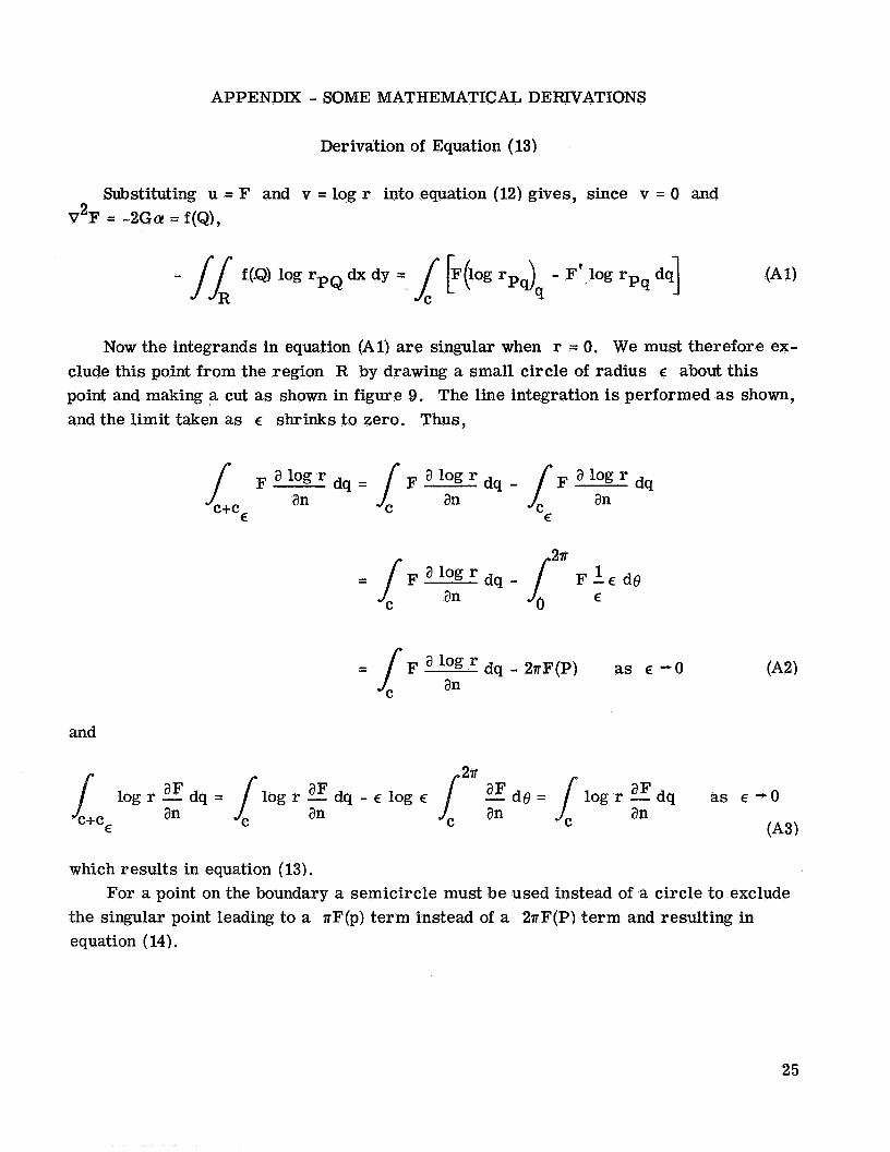
APPENDIX - SOME MATHEMATICAL DERIVATIONS

Derivation of Equation (13)

Substituting u = F and v = log r into equation (12) gives, since v = 0 and 2 V F = -2Ga = f(Q),

Now the integrands in equation (Al) are singular when r = 0. We must therefore exclude this point from the region R by drawing a small circle of radius E about this point and making a cut as shown in figure 9. The line integration is performed a s shown, and the limit taken as E shrinks to zero. Thus,

2a 1 - F - € d e E

- / F a log dq - an

C

and

2n E d e = l o g r E d q as E -0 aF aF

an an an an log r - dq = log r - dq - E log E

(A3)

which results in equation (13).

the singular point leading to a aF(p) term instead of a 2nF(P) term and resulting in equation (14).

For a point on the boundary a semicircle must be used instead of a circle to exclude

25

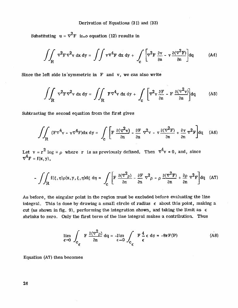
Derivation of Equations (3 1) and (33)

Substituting u = V F irkGa equation (12) results in 2

v dxdy = //vV41? dx dy + 1 [.“F - v acv2F)]dq an (A41 an

C

Since the left side is-symmetric in F and v, we can also write

F@gdq (A5) /L FV4vdxdy+ [&E- /l V2FV2v dx dy = an an

Subtracting the second equation from the first gives

2 av 2 1 - - - v v - v a(v2v) aF 2 a(v F, + - V F dq (A6) an an an

4 4 (FV v - vV F)dx dy =

2 4 Let v = r log p where r is as previously defined. Then V v = 0, and, since 4 v F =f(x,y) ,

As before, the singular point in the region must be excluded before evaluating the line integral. This is done by drawing a small circle of radius E about this point, making a cut (as shown in fig. 9), performing the integration shown, and taking the limit as E shrinks to zero. Only the first term of the line integral makes a contribution. Thus

Equation (A7) then becomes

26

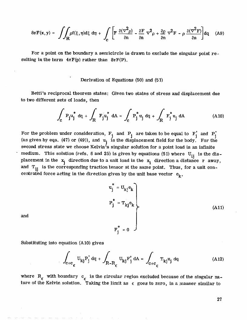
p + $ V 2 F - p a(v2F)] dq (A9) an an an an

8aF(x,y) =

For a point on the boundary a semicircle is drawn to exclude the singular point resulting in the term 4aF(p) rather than 8wF(P).

Derivation of Equations (50) and (51)

Betti's reciprocal theorem states: Given two states of stress and displacement due to two different sets of loads, then

* P.U. J 3 dq + F.u* J J dA = l P : u . J J dq + F:u. J J dA

For the problem under consideration, F. and P. are taken to be equal to F.' and P' J 3 3 3 (as given by eqs. (47) or (49)), and u. is the displacement field for the body. For the

3 second stress state we choose Kelvin's singular solution for a point load in an infinite

* medium. This solution (refs. 6 and 25) is given by equations (51) where U.. is the dis- 1J

placement in the xj direction due to a unit load in the xi direction a distance r away, and T.. is the corresponding traction tensor at the same point. Thus, for a unit con-

13 centrated force acting in the direction given by the unit base vector ek,

*

"j = u k j e k 7

and

*

* F. = 0

3

Substituting into equation (A10) gives

U kj P 'dq j + U kJ .F! 3 dA = Tkjy dq

where RE with boundary cE is the circular region excluded because of the singular na- ture of the Kelvin solution. Taking the limit as E goes to zero, in a manner similar to

27

what was done in deriving equation (131, results in equation (50). The term Xui(P) comes from the term on the right hand side of equation (A12).

Equation (52) is obtained as follows. The elastic part of the total strains is given by

Eij e - - Eij - Eij P - tiij m (A 13)

Now

(A 14) * u . .~ . . dA

13 9

where the starred fields refer, as before, to Kelvin's singular solution. Equation (A14) follows from Hooke's law. Substituting equation (A13) into equation (A14) and using the strain displacement relations, the equilibrium equations for the starred stress field, and the divergence theorem result in

* * * ui Fi dA

(A 15) u.u..n. dq - / .;(E: + tiijfl)dA = / u. 1 u..n. 1J J dq +

R -RE C+CE

Utilizing the relations

* * uij r j = P i = T ki e k]

J * u i j = Cijkek

where Tki, uki, and a re defined in equations (51) and (531, gives

Taking the limit as E approaches zero results in equation (52).

28

REFERENCES

1. Sternberg, Wolfgang J. ; and Smith, Turner L. : Theory of Potential and Spherical Harmonics. Toronto Press, 1946.

2. Kupradze, V. D. (H. Gutfreund, trans. ): Potential Methods in the Theory of Elasticity. Israel Program for Scientific Translations, 1965.

3. Jaswon, M. A. : Integral Equation Methods in PotentialTheory. I. Proc. Roy. i%C.

(London), Ser. A, vol. 275, no. 1360, Apr. 20, 1963, pp. 23-32.

4. Symm, G. T. : Integral Equation Methods in Potential Theory. 11. Proc. Roy. SOC. (London), Ser. A, vol. 275, no. 1360, Apr. 20, 1963, pp. 33-46.

Rep. MA-51, National Physics Lab., Dec. 1964.

Classical Elastostatics. Quart. Appl. Math., vol. 25, no. 1, Apr. 1967,

5. Symm, 6. T. : Integral Equation Methods in Elasticity and Potential Theory.

6. Rizzo, Frank J. : An Integral Equation Approach to Boundary Value Problems of

pp. 83-95.

7. Timoshenko, S. ; and Goodier, J. N. : Theory of Elasticity. Second ed. McGraw- Hil l Book Co., Inc., 1951, p. 258.

8 . Sokolnikoff, Ivan S. : Mathematical Theory of Elasticity. Second ed. McGraw-Hill Book eo., Inc. , 1956, p. 109.

9. Jaswon, M. A. ; and Ponter , A. R. : An Integral Equation Solution of the Torsion Problem. Proc. Roy. SOC. (London), Ser. A, vol. 273, no. 1353, May 7, 1963, pp. 237-246.

10. Mendelson, Alexander: Plasticity: Theory and Application. Macmillan Co. , 1968. 11. Roberts, Ernest Jr. ; and Mendelson, Alexander: Analysis of Plastic Thermal

Stresses and Strains in Finite Thin Plate of Strain-Hardening Material. N D-2206, 1964 ~

12. Segedin, C. M.; and Brickell, . G. A. : An Integral Equation Method for A Corner Plate. Am. SOC. Civil Eng. , Structural Fiv. J. , vol. 94, no.

lane Elasto-Plastic Analysis of V-Notched

1, 1968, pp. 41-52.

e Under Bending by tegral Equation Method hesis, Univ. Toledo, 1972.

ter; Mendelson, Alexander; and Albers, Lynn, U. : Application of Boundary Integral Method to Elastic Analysis of V-Notched Beams. NASA TN D-7424, 1973.

15. Rim, Kwan; and Henry, Allen S. : An Integral Equation Method In Plane Elasticity, NASA CR-779, 1967.

29

16. Rim, Kwan; and Henry, Allen S. : Improvement of an Integral Equation Method in Plane Elasticity Through Modification of Source Density Representation. NASA CR-1273, 1969.

17. Jaswon, M. A. ; Maiti, M. ; and Symm, 6. T. : Numerical Biharmonic Analysis and Some Applications. Int. J. Solids Structures, vol. 3, no. 3, 1967, pp. 309-332.

18. Szmodits, K. : Solution of the First Basic Problem of the Theory of Elasticity with Real Potentials. Acta Tech. Acad. Scientiarum Hungaricae, vol. 68, no. 3-4, 1970, pp. 353-358.

19. Massonet, C. E. : Numerical Use of Integral Procedures. Stress Analysis: Recent Developments in Numerical and Experimental Methods. Zienkiewicz, 0. C. and Holister, G. S., eds. John Wiley & Sons, Inc., pp. 198-235.

20. Liu, H. K. ; and Martenson, A. J. : Structural Analysis by Integral Techniques - Plane Elasticity Problems. Rep. 69-C-366, General Electric Co. , Oct. 1969.

21. Liu, H. K. ; and Martenson, A. J. : Structural Analysis by Integral Techniques. Three Dimensional Problems with or without Thermal Gradient Effects. Rep. 70- C-148, General Electric Co. Apr. 1970.

22. Liu, H. K . : Saint 2: Structural Analysis by Integral Techniques. II - Axially Sym- metric Stress Distribution. Rep. 7 l-C -024, General Electric Co. , Dec. 1970.

23. Oliveira, E. R. A. : Plane Stress Analysis by a General Integral Method. Am. SOC.

Civil Eng., Eng. Mech. Div. J. vol. 94, 1968, pp. 79-101.

24. Fung, Y. C. : Foundations of Solid Mechanics. Prentice-Hall, Inc., 1965.

25. Love, A. E. H. : A Treatise on the Mathematical Theory of Elasticity. Fourth ed. Dover Publ. , 1944.

26. Rizzo, F. J. ; and Shippy, D. J. : A Formulation and Solution Procedure for the General Non-Homogeneous Elastic Inclusion Problem. Int. J. Solids Structures, vol. 4, no. 12, 1968, pp. 1161-1179.

27 ~ Walker, George E. , Jr. : A Study of the Applicability of the Method of Potential to Inclusions of Various Shapes in Two- and Three-Dimensional Elastic and Thermo- elastic Stress Fields, Ph. D. Thesis, Univ. Washington, 1969.

28. Bamford, W. : Numerical Solution Accuracy for the Direct Potential Method. Rep. SM-66, Carnegie-Mellon Univ. , May 197 1.

29. Riccardella, P. C. : An Improved Implementation of the Boundary-Integral Technique for Two-Dimensional Elasticity Problems. Rep. SM-72 -26, Carnegie-Mellon Univ. , Sept. 1972.

30

30. Cruse, T. A. : Numerical Evaluation of Elastic Stress Intensity Factors by the Boundary-Integral Equation Method. The Surface Crack; Physical Problems and Computational Solutions. ASME, 1972, pp. 153- 170.

31. Marcal, P. V. : A Stiffness Method for Elastic-Plastic Problems. Int. J. Mech. Sci., vol. 7, 1965, pp. 229-238.

32. Marcal, P. V. : A Comparative Study of Numerical Methods of Elastic-Plastic Analysis. AIAA J. , vol. 6, no. 1, Jan. 1968, pp. 157-158.

33. Swedlow, J. L. : A Procedure for Solving Problems in Elasto-Plastic Flow. Rep. SM-73, Carnegie-Mellon Univ., Sept. 1971.

34. Swedlow, J. L. ; and Cruse, T. A. : Formulation of Boundary Integral Equations for Three-Dimensional Elasto-Plastic Flow. Int. J. Solids Structures, vol. 7 , no. 12, 1971, pp. 1673-1683.

35. Cruse, T. A. : Numerical Solutions in Three Dimensional Elastostatics. Int. J. Solids Structures, vol. 5, no. 12, 1969, pp. 1259-1274.

36. Cruse, T. A. ; and VanBuren, W. : Three Dimensional Elastic Stress Analysis of a Fracture Specimen with a Crack. Rep. SM-21, Carnegie-Mellon Univ. , Jan. 1970.

37. Deak, Alexander L. : Numerical Solution of Three-Dimensional Elasticity Problems for Solid Rocket Grains Based on Integral Equations. Volume I: Integral Equation Formulations. Rep. MSNW-72 -68- 1, Mathematical Sciences Northwest, Inc. (AFRPL-TR-71-140-Vol. 1, AD-737123), Feb. 1972.

38. Cruse, T. A. ; and Rizzo, F. J. : A Direct Formulation and Numerical Solution of the General Transient Elastodynamic Problem - I. J. Math. Anal. Application, vol. 22, no. 1, Apr. 1968, pp. 244-259.

39 ~ Cruse, T. A. : A Direct Formulation and Numerical Solution of the General Tran- sient Elastodynamic Problem - 11. J. Math. Anal. Application, vol. 22, no. 2, May 1968, pp. 341-355.

Appl. Math., vol. 27, no. 1, Apr. 1969, pp. 57-65. 40. Kanwal, R. P. : Integral Equations Formulation of Classical Elasticity. @art.

. J. : An Application of the Correspondence Principle of J. Appl. Math., vol. 21, no. 2, Sept. 1971, inear Viscoelasti

pp. 321-330.

enjumea, R.; andsikarskie, D. L.: the Solution of Plane, Orthotropic Elas- roblems by an egral Method. J. Appl. Mech. vol. 94, no. 3, Sept.

1972, pp. 801-808.

31

43. Cruse, T. A. ; and Swedlow, J . L. : Interactive Program for Analysis and Design Problems in Advanced Composite Technology. Carnegie-Mellon Univ. (AFML - TR-7 1-268, AD-739560), Dee. 197 1.

44. Ponter, A. R. S. : An Integral Equation Solution of the Inhomogeneous Torsion Problem. SIAM J. Appl. Math,, vol. 14, no. 4 , July 1966, pp. 819-830.

32

Number of equations,

n

~~

aFrom ref. 9.

Dimensionless Maximum dimensionless torsional rigidity, shear stress,

'm D

Figure 1. - Interior and boundary modal points.

Figure 2. - Region R, boundary curve c, and geometric quantities entering into boundary integrals.

33

1

F ' - 0 X

Figure 3. - Square plate under uni form tension. Exact solution: o = 60 = 1. Boundary-integral solution, % = 1.h.

.16

.08

0

a r-

2

0 -.08 .- U

=-. c VI VI aa I c cn

.- -.le

-. 21

-. 32

-. 4

Y

0 Boundary integral Finite difference

0 .5 1.0 X

Figure 4. - Thermal stress in square plate; o,, at y = 0 as function of x. (One quadrant of plate shown,)

-. 5

-.4 -. 3

-. 2

-. 1

a 0 P . I

.2

. 3

.4

.5 -1.2 -1.0 -.8 -.6 -.4 -.2 0 .2 .4 .6 .8 1.0 1.2

X

Figure 5. - Growth of the plastic zone size wi th load for a l inear strainhardening specimen with a loo edge notch subjected to pure bending; plane strain; ratio of slope of strainhardening l ine to elastic line, 0.05 (from ref. 13).

34

P(q)

(a) Stress vector at inter ior point M due to fictitious load distribution.

I .X

(bl Boundary forces and variables entering into

Figure 6. Geometric and force variables enter-

f ictit ious load formulation.

ing into fictitious load formulation (eqs. (43) and (44)).

I I I 113 213 1

-. 4; X

Figure 7. - Unit cube under axial load for 12 surface elements.

35

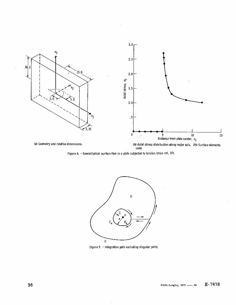
3.0r

0 5 10 15 Distance from plate center, x1

(b) Axial stress distribution along major axis. 256 Surface elements (a) Geometry and relative dimensions. used.

Figure 8. - Semielliptical surface flow in a plate subjected to tension (from ref. 37).

Figure 9. - Integration path excluding singular point.

36 NASA-Langley, 1973 - 32 E- '7478

NATIONAL AERONAUTICS AND SPACE ADMINISTRATION WASHINGTON, D.C. 20546 POSTAGE AND FEES PAID

NATIONAL AERONAUTICS AND OFFIC IAL BUSINESS SPACE ADM I NlSTRATlON

PENALTY FOR PRIVATE USE $300 SPECIAL FOURTH-CLASS RATE 451

BOOK

POSTMASTER : If Undeliverable (Section 158 Postal Ifannal) Do Not Return

NASA

‘“The aeronautical and space activities of the United States shall be conducted so as t o contribute . . . t o the expansion of human knowledge of phenomena in the atmosphere and space. The Administration shall provide for the widest practicable and appropriate dissemination of information concerning its activities and the results thereof.”

-NATIONAL AERONAUTICS AND SPACE ACT OF 1958

SCIENTIFIC AND TECHNICAL PUBLICATIONS TECHNICAL REPORTS: Scientific and technical information considered important, complete, and a lasting contribution to existing knowledge.

TECHNICAL TRANSLATIONS : Information published in a foreign language considered to merit NASA distribution in English.

TECHNICAL NOTES: Information less broad in scoDe but nevertheless of imoortance as a

PUBLICAT1oNS: Information derived from or of value to NASA activities.

contribution to existing knowledge.

TECHNICAL MEMORANDUMS: Information receiving limited distribution because of preliminary data, security classifica- tion, or other reasons. Also includes conference proceedings with either limited or unlimited distribution.

CONTRACTOR REPORTS: Scientific and technical information generated under a NASA contract or grant and considered an important contribution to existing knowledge.

Publications include final reports of major projects, monographs, data compilations, handbooks, sourcebooks, and special bibliographies.

TECHNOLOGY UTILIZATION PUBLICATIONS: Information on technology used by NASA that may be of particular interest in commercial and other- non-aerospace applications. Publications include Tech Briefs, Technology Utilization Reports and Technology Surveys.

Details on the availability of these publications may be obtained from:

SCIENTIFIC AND TECHNICAL INFORMATION OFFICE

N A T I O N A L A E R O N A U T I C S A N D SPACE A D M I N I S T R A T I O N Washington, D.C. 20546

boundary-integ al methods in elasticity and plasticity … · bqundary-integ~l methods in...

Documents