Building up to IFRS 17Understanding the new reporting standard for insurance contracts

August 2017

Introduction

IFRS 17 is an accounting standard, but it’s not just for accountants. The complexity of calculations and amount of judgement required to inform decisions on methodology and processes mean that actuarial teams will be involved in financial reporting to a much greater extent than ever before. But is it just some monster that can be left to the techies? Much as some might like to hope so, we wouldn’t agree:

• Profit emergence will be different and, with less opportunity to offset less profitable products within a portfolio or against reinsurance treaties, a review of product ranges, pricing and reinsurance structures may be needed.

• Interaction of the financial and regulatory statements will require careful consideration in terms of the likely different outcomes for profit emergence, capital and dividend paying capability.

• Analysing the liabilities in the required format and grouping model points will take much more time and effort compared to current practices, and managing the grouped data in the future in line with the reporting requirements will also mean an ongoing material effort.

After more than 20 years in the planning and a “go-live” date set as at 1 January 2021, IFRS 17: Insurance Contracts is finally about to fundamentally change financial reporting for insurers.

• Existing systems will need a potentially major overhaul both to cater for the complexity of calculating the required figures and to manage the data requirements.

• Remuneration packages may need to be re-stated (and potentially re-negotiated).

• Education programmes will be needed to ensure that users of financial statements are interpreting the detail appropriately.

• It will introduce new dynamics and resource challenges in the reporting functions as actuaries will be much more involved in the production of the revenue statements rather than their more traditional involvement with the balance sheet.

With these points in mind, we hope you will find this paper useful in helping you not only to understand the technicalities of the standard, but importantly to identify the areas of focus required from your teams during implementation.

If you would like to discuss any of the information in this paper further please contact a member of our team.

2

John McKenzie Head of Insurance Transfers and Reporting Servicejohn.mckenzie@hymans.co.uk

ContentsIntroduction 2How to read this paper 4High Level Overview 51 Unbundling and Contract Boundaries 92 The Building Block Approach 103 The Variable Fee Approach 184 The Premium Allocation Approach 205 Transition 216 Accounting Presentation 24Appendix – Case studies 28

Emma McWilliam Head of Life and Financial Servicesemma.mcwilliam@hymans.co.uk

3

If you have little need to gain detailed knowledge of the workings of IFRS 17 you may find the High Level Overview sufficient to gain a flavour of the standard. However, you may also find the body of the report, which sets out the framework more fully, to be helpful.

Go to page 5

How to read this paper

This paper summarises the key parts of the IFRS 17 standard. We do not intend to cover all details of the standard, but instead draw out the main aspects in order to focus attention. It is written for professionals working in UK life insurers or in companies holding insurance contracts.

IFRS 17 is not an easy topic and not everyone will need an in depth understanding of it. We have therefore structured this paper in a way which will prove useful to different levels of reader interest:

Reliances and limitationsThis paper has been compiled by Hymans Robertson LLP and is based upon our current understanding of IFRS 17: Insurance contracts issued in May 2017. It is designed to be a general information summary and may be subject to change. This information is not to be interpreted as an offer or solicitation to make any specific decisions. The material and charts included herewith are provided as background information for illustration purposes only. The examples provided are based on our interpretation of the standard and have been simplified where possible. As such, they should not be taken as a definitive analysis of the subject covered or specific to the circumstances of any particular insurer or reinsurer. The information contained is not intended to constitute advice, and should not be considered a substitute for specific advice in relation to individual circumstances. Where the subject of this document involves legal issues you may wish to take legal advice. Hymans Robertson LLP accepts no liability for errors or omissions or reliance on any statement or opinion.

For simplicity, we refer to an insurer in this paper as any entity that issues insurance or reinsurance products, the measurement of which falls within scope of IFRS 17.

Overview Digging into the detail Worked examples

The body of the report is aimed more at you if you are of a technical bent, but are not a practitioner. We have, where possible, provided a simpler description in more common language. Otherwise, we have maintained consistency and a link to the jargon which practitioners will employ and have provided definitions in the glossary.

Go to page 9

The Appendix to the report sets out some detailed worked examples of how the standard works in practice. If you are a practitioner this will appeal to you to reinforce your working knowledge. However, we believe that a quick look at the Appendix will be useful for everyone, if only to get a feel for the complexity of the process which will be required.

Go to page 28

4

2021

High Level Overview

Background and timetable to implementation There is currently no single consistent accounting standard for insurance contracts and a range of practices are currently used for IFRS reporting. IFRS 4: Phase I issued in 2004 introduced some improvements to disclosure requirements and measurement, but insurers were largely permitted to continue with previous accounting practices. Phase II of the IFRS 4 project, completed with the issuance of IFRS 17, aims to harmonise accounting practices across the industry by addressing the weaknesses in current practices and improving the comparability of information for users of financial statements. The new standard comes into full force on 1st January 2021, but insurers will be expected to restate at least one year of comparatives.

IASC (now IASB) approves project

on insurance accounting

IFRS 4 Phase I issued

2010 and 2013 exposure draft issued

IFRS 17 published

Production of comparatives

IFRS 17 goes live

1997 2004 2017 2020

Implementation

IFRS 17 has been more than twenty years in the making and will radically change the financial reporting for insurers. This will require the involvement of actuarial teams to a much greater extent than ever before. Despite the years of build-up to the new standard, many companies are only now beginning to think about the potential changes they will need to make and how they will actually fit into their existing processes.

OverviewThis part of the paper gives a flavour of the standard for those who don’t need detailed insight

5

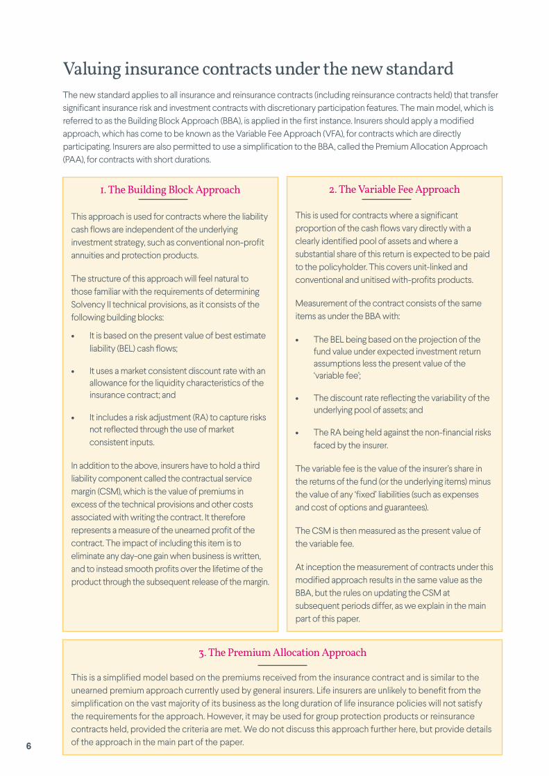
1. The Building Block Approach

This approach is used for contracts where the liability cash flows are independent of the underlying investment strategy, such as conventional non-profit annuities and protection products.

The structure of this approach will feel natural to those familiar with the requirements of determining Solvency II technical provisions, as it consists of the following building blocks:

• It is based on the present value of best estimate liability (BEL) cash flows;

• It uses a market consistent discount rate with an allowance for the liquidity characteristics of the insurance contract; and

• It includes a risk adjustment (RA) to capture risks not reflected through the use of market consistent inputs.

In addition to the above, insurers have to hold a third liability component called the contractual service margin (CSM), which is the value of premiums in excess of the technical provisions and other costs associated with writing the contract. It therefore represents a measure of the unearned profit of the contract. The impact of including this item is to eliminate any day-one gain when business is written, and to instead smooth profits over the lifetime of the product through the subsequent release of the margin.

2. The Variable Fee Approach

This is used for contracts where a significant proportion of the cash flows vary directly with a clearly identified pool of assets and where a substantial share of this return is expected to be paid to the policyholder. This covers unit-linked and conventional and unitised with-profits products.

Measurement of the contract consists of the same items as under the BBA with:

• The BEL being based on the projection of the fund value under expected investment return assumptions less the present value of the ‘variable fee’;

• The discount rate reflecting the variability of the underlying pool of assets; and

• The RA being held against the non-financial risks faced by the insurer.

The variable fee is the value of the insurer’s share in the returns of the fund (or the underlying items) minus the value of any ‘fixed’ liabilities (such as expenses and cost of options and guarantees).

The CSM is then measured as the present value of the variable fee.

At inception the measurement of contracts under this modified approach results in the same value as the BBA, but the rules on updating the CSM at subsequent periods differ, as we explain in the main part of this paper.

3. The Premium Allocation Approach

This is a simplified model based on the premiums received from the insurance contract and is similar to the unearned premium approach currently used by general insurers. Life insurers are unlikely to benefit from the simplification on the vast majority of its business as the long duration of life insurance policies will not satisfy the requirements for the approach. However, it may be used for group protection products or reinsurance contracts held, provided the criteria are met. We do not discuss this approach further here, but provide details of the approach in the main part of the paper.

Valuing insurance contracts under the new standardThe new standard applies to all insurance and reinsurance contracts (including reinsurance contracts held) that transfer significant insurance risk and investment contracts with discretionary participation features. The main model, which is referred to as the Building Block Approach (BBA), is applied in the first instance. Insurers should apply a modified approach, which has come to be known as the Variable Fee Approach (VFA), for contracts which are directly participating. Insurers are also permitted to use a simplification to the BBA, called the Premium Allocation Approach (PAA), for contracts with short durations.

6

What does IFRS 17 mean for your business?So what does all this mean to you? Our introduction has highlighted some of the impacts the new standard will have on your business in terms of profit emergence, remuneration and systems and processes. In this section, we draw out the details of some of the key points raised.

1. Change in profit emergence

One important result of IFRS 17 is the smoothing of profit over time. The profit of insurance business is known to be lumpy in nature with the impact of new business written and changes in valuation assumptions having an immediate effect on the profit and loss (P&L) statement. This has been expressed by some as an issue for investors who generally prefer predictable profits that are easy to forecast. IFRS 17 addresses this by requiring firms to hold a CSM, which has the impact of smoothing profits in line with the provision of services.

The CSM is reduced over the lifetime of the contract, releasing profit which is recognised in each reporting period. The impact on profitability due to changes to future cash flow assumptions (such as mortality/morbidity assumptions) are also smoothed over time. This is achieved by ’unlocking’ the CSM to offset the liability impact. On the other hand the effect of incurred claims and financial assumption changes (under the BBA) are recognised immediately in P&L/Other Comprehensive Income (OCI).

Furthermore, an immediate impact will occur at the point of transition when the balance sheet moves from IFRS 4 to IFRS 17. For some contracts, such as annuities, this has the effect of writing back part of the profits already declared under IFRS 4, so that it will be earned again in the future through the release of the CSM. The implications of this on tax are being discussed with HM Revenue & Customs. The impact of this on dividends will also need to be considered, although we would note that for UK life insurers these impacts are not expected to directly affect distributable surplus out of which dividends are paid, as these are based on the Solvency II balance sheet. There is no doubt that these changes to profit emergence will affect remuneration.

We look at the CSM mechanism and the impact it will have on the profitability of contracts in greater detail in the main part of the paper.

2. Grouping of model points into portfolios

Insurers will have to make a decision on the way contracts are grouped for measuring the CSM. This will have

implications on the shape of profit emergence for these contracts - in particular as insurance and reinsurance contracts must be grouped separately. This analysis will require time and effort, though the International Accounting Standards Board (IASB) has aimed to reduce the onus of the process by emphasising the use of a top-down approach.

Insurance contracts should be grouped by line of business and then into three further groups depending on their expected profitability. These are:

1. A group of contracts that result in a loss at inception;

2. A group of contracts that have no significant risk of making a loss; and

3. A group of other profitable contracts.

The measure of profitability is left to the individual insurer to decide, as is the level of testing required to determine whether contracts have a significant risk of making a loss. The groups are then further divided into portfolios that contain contracts which were written no more than a year apart. The recognition of profit is asymmetric for profitable contracts and those written at a loss, with the latter being recognised immediately in the P&L.

3. Overhaul of systems

We expect that much of the infrastructure insurers have put into place for Solvency II can be recycled for IFRS 17. However the timescales required for producing IFRS reporting in comparison to Solvency II may mean that these systems and processes are put under increasing pressure, and significant updates to systems may be required in order to produce the amount of information needed at the right time. One key difference between IFRS and Solvency II is that Solvency II does not require the tracking of historical information for future reporting cycles. For example the rules around CSM calculation mean insurers will need to hold a database of historical discount rates and track the groups of contracts until they come off the books. The management and analysis of this data and the associated cost could become substantial.

7

IFRS 17 Solvency II

Approach Principles based Prescriptive

Non-financial assumptions in the BEL

Calculation based on best estimate assumptions.

Calculation based on best estimate assumptions.

Discount rate For BBA, derived from an appropriate reference asset portfolio, adjusted to reflect the characteristics of the liability cash flows.

For VFA, discount rates should reflect the variability of the underlying pool of assets.

Specified risk free curve.

Discount rate only adjusted where matching adjustment or volatility adjustment criteria satisfied.

Risk adjustment Held to cover the uncertainty associated with non-financial risks faced by the insurer.

Flexibility on calculation approach.

Risk margin is intended to represent the amount an insurance company would need to hold in order to wind up and transfer its obligation to another party after a stress scenario occurring. It is calculated using a cost of capital approach. It is added to the BEL to give the Technical Provisions.

Profit recognition Deferred and smoothed. Total liabilities are increased by holding the CSM.

Recognised immediately in Own Funds.

Grouping of contracts for measurement and disclosure

Grouping by profitability criteria and year of issue, resulting in portfolios with similar risk characteristics.

No offsetting of profits and losses within product groups.

No netting off of reinsurance contracts.

Grouping by homogeneous risk groups, which are collections of policies with similar risk characteristics.

No netting off of reinsurance contracts.

Historical tracking of experience

Required to attribute profits via CSM or directly to P&L.

Re-calculation of the CSM at the start of the year may be required to attribute revenue.

Not directly required for reported items.

Comparison with Solvency IIAlthough IFRS17 and Solvency II share a common starting point of establishing a best estimate view of the liabilities, there are key differences in the computational effort and in the comparability of many of the outputs.

4. The complexity at transition

Transition is another mammoth task insurers will face. The CSM will have to be determined at the transition date as if the standard has been in place since contract inception. When measured retrospectively in full, this means that the CSM at transition is the value that would have been calculated at inception run down to the transition date.

The challenge with this is that insurers are unlikely to have stored valuation assumptions when contracts were priced. Furthermore, insurers are not permitted to use the benefit of hindsight to calculate the CSM at inception. However the standard does provide some relief where full retrospective measurement is not possible.

8

1. Unbundling and Contract Boundaries

Before insurers can work on the measurement of insurance contracts or indeed decide on which measurement model should be used for each contract type, an assessment needs to be made of the contract terms and whether they are covered by IFRS 17.

Unbundling components of insurance contracts

The criteria for separating the insurance component from other non-insurance components of contracts (unbundling) has changed from current practice. Where a contract contains components which would fall under the scope of another IFRS if treated in isolation, such as an investment component, it should be unbundled and measured under the relevant IFRS as if it were separate, but only if the following are satisfied:

• The component is not highly interrelated to the insurance component in that each component can be valued even if the other were not present or the policyholder can benefit from one component without the other being present; and

• The separated component is readily available for purchase in the same market or jurisdiction.

If these requirements are satisfied, investment components which can be treated in isolation should be measured under the standard IFRS 9: Financial Instruments. Investment contracts with no significant

insurance element, such as unit-linked savings contracts, will also fall under IFRS 9: Financial Instruments. Distinct goods or non-insurance services which form a part of the contract should be separated and measured under IFRS 15: Revenue from Contracts with Customers.

Contracts which have previously been unbundled, but do not satisfy the new unbundling criteria, will need to be re-bundled and accounted for under IFRS 17.

Definition of a contract boundary

The valuation of contracts under IFRS 17 should only take into account cash flows up to their contract boundaries. This concept will be familiar to practitioners of Solvency II and is the point at which coverage is no longer provided or the issuer of the contract has the right to revalue the benefits underlying the contract and reassess the price. The boundary therefore acts as a distinction between cash flows relating to the existing contract from those relating to future contracts.

The definition of contract boundaries is similar under Solvency II and in most circumstances applying the two definitions will end in the same result. However, the requirement to unbundle non-insurance components under IFRS 17 may cause a different result to arise.

Insurers need to determine which part of a contract falls under the new standard and at what point in the future the contract ends

Digging into the detailThis part of the paper walks through in more detail the technicalities of the IFRS 17 standard

9

2. The Building Block Approach

The measurement of liabilities under this approach is made up of four parts, as shown in figure 1. The present value of future cash flows and the risk adjustment make up what the standard refers to as the fulfilment cash flows of the contract.

Also known as the general model, the Building Block Approach is used for products where cash flows do not vary in line with returns from a defined pool of assets, such as conventional non-profit annuities and protection business.

Estimation of future cash flowsThe starting point of the Building Block Approach is an estimate of future cash flows, calculated on a best estimate basis, which represents the expected value (the probability-weighted mean) of the full range of possible outcomes. The cash flows should not reflect the net effect of two or more components occurring. In particular, they should not include a margin for uncertainty or be netted off against reinsurance cash flows.

Reinsurance contracts held are measured separately under IFRS 17, where the present value of future cash flows should also take into account the expected losses on default of the reinsurer.

Attributable acquisition costs should be allocated over the contract term in a way that reflects the transfer of services under the contract rather than being reflected as and when they are incurred. In this way, they form a part of the future contract cash flows. Economically this is broadly equivalent to deferred acquisition costs under current accounting practices.

Figure 1. Components of the Building Block Approach

Fulfilment cash flows

Source: IASB and Hymans Robertson, for illustration purposes

Includes all future inflows and outflows

Cash flows are discounted to reflect the time value of money

Reflects the uncertainty of future cash flows

Runs off over the policy coverage period. Established so that no day one gain is made

Future cash flows

Risk adjustment

Time value

Contractual Service Margin

10

Discount ratesDiscount rates are applied to the best estimate cash flows to calculate the present value of the contract. The general principle is that discount rates should be consistent with the characteristics of the future liability cash flows. They should therefore be based on current observable prices in the market for assets which hold the same characteristics as the liabilities in terms of timing, currency and liquidity.

A. The top-down approach starts with a yield curve based on the current market rates of return from either an actual portfolio of assets held by the company or a reference portfolio. Estimates of the factors which are not passed on to policyholders through the insurance contracts (or which in the words of the standard are ‘not relevant’) should be deducted from the observed rates, as shown in figure 2. The default adjustment shown covers expected default and downgrades of the assets. There is no need to include adjustments for the risk of the company being unable to fulfil its obligations or for differences in liquidity characteristics between the asset and liability portfolio.

Figure 2. Discount rate calculation under the Building Block Approach

IFRS discount

rate

Yield curve based on actual or

reference asset

portfolio

Default adjustment

Mismatch adjustment

Risk free rate

Illiquidity premium

Top down approach Bottom up approach

Source: Hymans Robertson, for illustration purposes

B. The bottom-up approach starts with a risk-free yield curve and adds on an illiquidity premium, i.e. an adjustment that reflect the differences between the liquidity characteristics of risk-free assets and those of the insurance contracts. In the bottom-up approach the differences between the liquidity characteristics of the risk free curve and the insurance contracts should be allowed for.

It is expected that both these approaches should result in the same IFRS discount rate being derived. However, in practice, the results may be different as a result of the approximations in determining the adjustments required. It is also important to note that the adjustments will differ depending on the type of insurance contract being measured.

There are two methodologies which can be used to determine discount rates - the top down approach and the bottom up approach.

11

Figure 3. Example calculation methods for the risk adjustment

Source: Hymans Robertson summary based on IASB website

Value at Risk (“VaR”)

This calculates the RA as the minimum increase in the expected liability value that is not exceeded with a given probability or level of confidence, over a given time period.

VaR

Conditional Tail Expectation (“CTE”)

Also referred to as tail value at risk. It calculates the RA as the amount on top of expected liability value which covers the average liability beyond a chosen VaR. This method is often chosen where outcome distributions are skewed or have fat tails.

CTE

Cost of Capital (“CoC”)

The cash flow losses at a chosen confidence level are calculated and adjusted for the time value of money. This capital amount is then multiplied by a cost of capital rate.

CoC

Risk adjustmentThe risk adjustment is held to cover the risk of future cash flows being different from the best estimate. It shares some similarities with the risk margin under Solvency II and should only include non-financial risks.

The risk adjustment is required to have the following characteristics:

• Risks with low frequency and high severity should result in a higher risk adjustment;

• For similar risks, contracts with longer durations should result in a higher risk adjustment;

• Risks with a wide probability distribution should result in a higher risk adjustment;

• The less that is known about the current estimate and the trend, the higher the risk adjustment should be; and

• To the extent that emerging experience reduces uncertainty, the risk adjustment should decrease.

Although the standard does not specify the methodology which should be used to calculate the risk adjustment, there were suggestions of possible methods in an earlier version of the IFRS 17 exposure draft.

Insurers are expected to use their judgement when it comes to choosing the appropriate methodology based on the characteristic requirements of the risk adjustment. For example, the IASB has stated that where the distribution of outcomes for the contracts is highly skewed, it may be more appropriate to use the conditional tail expectation or cost of capital methods.

Regardless of the approach adopted, companies have to calculate and disclose the equivalent level of confidence under the VaR method for the risk adjustment calculated. The level of confidence to which the risk adjustment should be calibrated is not specified in the standard and remains a choice for the individual insurer.

12

Andrew Scott Senior Life Consulting Actuary andrew.scott@hymans.co.uk

Ourview

The structure of the Building Block Approach is, on the surface at least, similar to that of the Solvency II balance sheet where the technical provisions are the sum of the best estimate liability and the risk margin. There are, however, important differences between the regulatory and accounting requirement, with IFRS 17 generally being much less prescriptive than Solvency II.

In general, the discount rates used for IFRS 17 purposes are not determined in the same way as Solvency II. The resulting rates are expected to be different. For annuity business, the rates can be measured as the sum of the risk-free rate and an illiquidity premium, which looks superficially similar to Solvency II as the sum of the risk-free rate and the Matching Adjustment. However, IFRS 17 states that the illiquidity premium should reflect the liquidity characteristics of the insurance contracts – whereas the Matching Adjustment reflects the characteristics of the backing assets. It seems likely that insurers will be able to use the “top down approach” to derive the illiquidity premium in the same way as they derive the Matching Adjustment – but this is only one of the options available to them and it may not be appropriate for every firm. Furthermore, where insurers choose not to use the EIOPA curves for IFRS 17, the risk free assumption will be different from Solvency II. IFRS 17 also requires the tracking of interest rates, which is something that is not required under Sovency II and could result in substantial system changes.

Similarly, one acceptable way of deriving the risk adjustment required by IFRS 17 might be to set it equal to the Solvency II risk margin – but, again this is just one of a number of possible approaches.

Harmonising the accounting and regulatory balance sheets might be the simplest approach for firms in terms of the processes and systems that will need to be built. However the design of both the risk margin and the Matching Adjustment have been criticised by various stakeholders, and firms may prefer an accounting treatment that better reflects the economics of their business.

The decision of whether or not to harmonise the balance sheets brings with it asset liability management considerations: if there are two different balance sheets, which one should the firm focus its efforts on? One pertinent example is that some firms have decided not to hedge the interest rate sensitivity of the Solvency II risk margin, partly on the grounds that doing so would destabilise their IFRS profits. There may be more desire to hedge the Solvency II risk margin if the IFRS balance sheet contains a risk adjustment which behaves in a similar manner.

13

Contractual Service MarginThe CSM represents a measure of the unearned profit in a contract. It should be measured at outset as the amount equal to the value of the premiums received or receivable minus the present value of the liabilities and costs associated with writing and servicing the contract. Such costs include directly attributable acquisition costs and commission.

Where the value calculated is positive, the margin is held as a liability item which results in zero day-one profit. It is then released and recognised in P&L over the term of the contract (or what the standard refers to as the coverage period) in a way which reflects the transfer of services.

If the figure is negative the contract is said to be onerous and represents an initial loss which should be recognised immediately in P&L. The CSM is then set to zero.

In this way, the treatment of a profit and a loss is asymmetric under IFRS 17, with the former being smoothed over the lifetime of the contract and the latter recognised immediately in the P&L. Therefore contracts (or portfolios of contracts) will need to be tracked to ensure the accounting treatment is correct in each future period as contracts may move from being onerous to profitable or vice versa.

2.4.1 Aggregation of contracts

The objective of the CSM is to recognise profit for an individual contract over a period that reflects the services provided by the contract. However, insurers are permitted to group policies to calculate the value of the CSM and set the pattern of its release provided this objective is met.

The release of the CSM, whether on a single contract or group of contracts, should be based on the number of “coverage units” provided in the period. The coverage units of a group of contracts reflects the amount of service provided and the duration of the contracts. It can therefore be based on the change in the number of policies inforce from one period to the next.

Contracts can be grouped if the cash flows of the group have similar sensitivities in terms of timing and amount to changes in key drivers of risk and have similar profitability at inception. In addition, the coverage period of the contracts should be similar and only contracts which are issued within one year apart may be grouped together (the annual cohort rule).

A top-down approach should be used to group contracts into portfolios, where they are first divided according to their product line and then further split into a minimum of three groups:

1. A group of contracts that are onerous at initial recognition;

2. A group of contracts that have no significant risk of becoming onerous; and

3. A group of other profitable contracts.

One way of testing whether a group of contracts has significant risk of becoming onerous is to look at the change in profitability (based on a measurement decided by the insurer) to future experience or assumption changes through sensitivity or scenario testing.

Where law or regulation constrains the ability for insurers to set a different price or level of benefit for different groups of contracts, insurers can choose to include these contracts in the same group for the purposes of IFRS 17. An example of this is contracts priced neutrally as a result of the European Union Gender Directive.

Some information will be lost when determining the margin on a grouped basis and the shape and timing of profit emergence, or whether an initial loss is recognised, will depend on the method adopted to aggregate contracts into a portfolio.

14

2.4.2 Unlocking the contractual service margin

Under the Building Block Approach, the underwriting profit of an insurance contract - which is the profit stemming from non-investment related sources - consists of the release of the CSM, the release of the risk adjustment and differences between actual and expected experience where these arise. IFRS 17 also refers to this as the insurance service result. In general, the CSM is expected to run off over the lifetime of a contract with the impact of experience resulting in immediate recognition in the P&L. However, there are some occasions where the CSM is “unlocked” or recalculated/adjusted to allow for changes in assumptions that impact future cash flows under the contract, such as mortality or morbidity. Where the CSM is adjusted, this will fully or partially offset the impact of the assumption change on the BEL and RA so that no (or a smaller) impact flows into the P&L.

Year9876543210 10

Profi

t

Initial profit signature basedon cash flow projection at t=0

Profit signature based onnew cash flow projection at

t=1 and unlocked margin

No profit atcontract inception

Figure 4 shows the profit signature for a sample portfolio of annuity-style contracts and the impact of an increase in base mortality. In this example, under the initial profit signature, profit is expected to run off over a period of 10 years, decreasing over time due to expected deaths in the portfolio. At the end of year 1, a change to heavier future mortality assumptions unlocks the CSM and spreads the increase in expected profits over the remaining service period.

If instead the future mortality assumptions decreased, then overall profit is expected to reduce. This reduction is spread over the lifetime of the contract in the same way. However, if the CSM is not large enough to absorb the decrease, then the ‘shortfall’ will be recognised as a loss immediately in the P&L.

Figure 4. Expected profit emergence of a portfolio of annuity-style contracts

Source: For illustration purposes, based on Hymans Robertson analysis

15

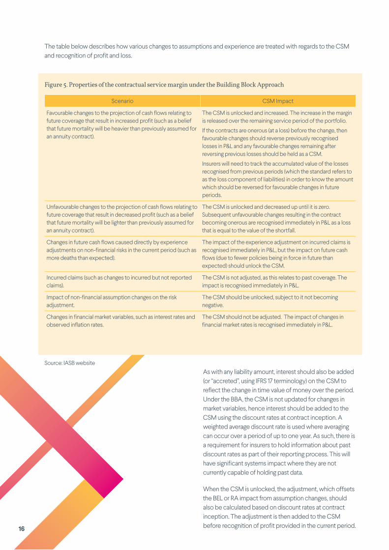
Scenario CSM Impact

Favourable changes to the projection of cash flows relating to future coverage that result in increased profit (such as a belief that future mortality will be heavier than previously assumed for an annuity contract).

The CSM is unlocked and increased. The increase in the margin is released over the remaining service period of the portfolio.

If the contracts are onerous (at a loss) before the change, then favourable changes should reverse previously recognised losses in P&L and any favourable changes remaining after reversing previous losses should be held as a CSM.

Insurers will need to track the accumulated value of the losses recognised from previous periods (which the standard refers to as the loss component of liabilities) in order to know the amount which should be reversed for favourable changes in future periods.

Unfavourable changes to the projection of cash flows relating to future coverage that result in decreased profit (such as a belief that future mortality will be lighter than previously assumed for an annuity contract).

The CSM is unlocked and decreased up until it is zero. Subsequent unfavourable changes resulting in the contract becoming onerous are recognised immediately in P&L as a loss that is equal to the value of the shortfall.

Changes in future cash flows caused directly by experience adjustments on non-financial risks in the current period (such as more deaths than expected).

The impact of the experience adjustment on incurred claims is recognised immediately in P&L, but the impact on future cash flows (due to fewer policies being in force in future than expected) should unlock the CSM.

Incurred claims (such as changes to incurred but not reported claims).

The CSM is not adjusted, as this relates to past coverage. The impact is recognised immediately in P&L.

Impact of non-financial assumption changes on the risk adjustment.

The CSM should be unlocked, subject to it not becoming negative.

Changes in financial market variables, such as interest rates and observed inflation rates.

The CSM should not be adjusted. The impact of changes in financial market rates is recognised immediately in P&L.

Figure 5. Properties of the contractual service margin under the Building Block Approach

The table below describes how various changes to assumptions and experience are treated with regards to the CSM and recognition of profit and loss.

As with any liability amount, interest should also be added (or “accreted”, using IFRS 17 terminology) on the CSM to reflect the change in time value of money over the period. Under the BBA, the CSM is not updated for changes in market variables, hence interest should be added to the CSM using the discount rates at contract inception. A weighted average discount rate is used where averaging can occur over a period of up to one year. As such, there is a requirement for insurers to hold information about past discount rates as part of their reporting process. This will have significant systems impact where they are not currently capable of holding past data.

When the CSM is unlocked, the adjustment, which offsets the BEL or RA impact from assumption changes, should also be calculated based on discount rates at contract inception. The adjustment is then added to the CSM before recognition of profit provided in the current period.

Source: IASB website

16

Elaine Murphy Senior Life Consulting Actuary elaine.murphy@hymans.co.uk

Ourview

The CSM is a new concept for UK insurers and will be an area that firms will want to spend time understanding during the implementation phase.

In general IFRS profits will be slower to emerge under IFRS 17 than under current accounting practices as the CSM is smoothed over the service period of the contract. The grouping of contracts into the profitability categories will mean that insurers are largely unable to net off profitable and unprofitable contracts against each other. This will likely result in larger losses to be recognised at inception if any unprofitable contracts are written. Similarly there will be no immediate gain (or loss) from reinsurance ceded. Therefore, the grouping of contracts is likely to be a key decision for firms and the shape and timing of profit emergence will depend on the way in which contracts have been aggregated into a portfolio.

Volatility from changes to valuation assumptions, such as future mortality and morbidity assumptions will be smoothed out through unlocking the CSM rather than immediate recognition in income. This means that resulting profits from positive changes will be slower to emerge than under current practices.

Firms should remember that these changes impact the presentation and timing of profits only – the underlying economics of the products is not changing and as such the introduction of the new standard is not expected to have an impact on the total underwriting profit of the existing book. That said, firms should consider carrying out reviews of both product pricing and reinsurance structures to ensure that both remain fit for purpose in the new environment and achieve their targeted profit profiles.

The total value of the CSM at the end of a period for a given portfolio is thus determined as follows:

• The CSM value at the start of the period; plus

• The CSM of any contracts, which have similar expected cash flows and profitability, added to the portfolio; plus

• The interest added on the margin during the reporting period; plus or minus

• The changes in the fulfilment cash flows relative to those expected to the extent that the CSM is not negative; plus or minus

• The effect of any currency exchange differences; minus

• An amount released for the transfer of services in the period, determined by the change in coverage units in the period, after allowing for amounts which adjust the CSM.

The appendix of this paper provides an example of how the CSM is updated at subsequent measurement.

2.4.3 Reinsurance contracts held

Insurers should also measure reinsurance contracts held that transfer significant insurance risk using IFRS 17. However unlike underlying insurance contracts, insurers should hold a CSM in respect of the reinsurance contracts regardless of whether a gain or a loss is made when the reinsurance is written. As a result the CSM can be negative for reinsurance contracts held. This effectively means there is no immediate gain or loss on entering a reinsurance contract.

17

Contracts can be measured using the Variable Fee Approach (or are ‘directly participating’) when:

• The contract explicitly specifies a clearly identified pool of underlying items (such as a fund or pool of financial assets) in which the policyholder participates, although the insurer need not hold these items;

• A substantial portion of cash flows from the contract will vary with changes in the fair value of the items;

• The policyholder will receive a substantial share of the returns from those items.

It is left to the insurer to make their own interpretation of how to define “substantial” under bullet points 2 and 3.

The link to the underlying items of a directly participating contract that satisfies the VFA is enforceable. Therefore, where there are no specified underlying items or if the insurer can modify the underlying items in a way which retrospectively changes its obligations to the policyholder, the contract does not satisfy the criteria for the VFA.

3. The variable fee approach

Subject to certain criteria, with-profits and unit-linked contracts can be measured under the variable fee approach. Insurers will have to decide at transition to IFRS 17 or at inception of new business whether a contract satisfies the appropriate criteria.

Insurers will have to determine at inception whether a contract satisfies the criteria for the VFA. Although eligibility may change throughout the contract term (for example if the value of guaranteed death benefits exceed the value of the assets underlying the contract, resulting in the second criteria not being met), the criteria do not need to be reassessed and the VFA can continue to be used. The VFA should be applied to the whole contract, even if the contract contains a portion of fixed cash flows which do not vary with the underlying items, to the extent that the components cannot be unbundled.

18

Measurement under the Variable Fee ApproachLike the BBA, the VFA consists of the same four liability items with:

• The best estimate liability cash flows based on the projection of the fund value (or value of the underlying items) under expected investment return assumptions, less the amount of the variable fee. The variable fee is equal to the insurer’s share of the return on the underlying items (such as the annual management charge of a unit-linked contract) minus any items arising from contract features which do not vary with the underlying items, such as expenses and the level of guarantees.

• A discount rate based on the expected return and variability of the specified underlying items. Where the policy also has items whose level is fixed and does not vary with the underlying items, the discount rate should be adjusted to allow for the characteristics of these cash flows. The single discount rate can then be applied to all the cash flows under the contract.

• The RA, similar to the BBA, should be held against the non-financial risks faced by the insurer.

• The CSM is then measured as the present value of the variable fee and is recognised in the same way as the BBA based on coverage units (eg: number of policies in force).

In future periods the CSM is adjusted with the effect of changes in the estimate of the variable fee. Therefore, unlike the BBA, changes in interest rate assumptions should unlock the CSM rather than be recognised immediately in P&L. This is because the changes will affect the amount of return on the underlying items and thus the variable fee. Furthermore, the interest added on to the CSM for each reporting period, should also reflect the current discount rates at the date of valuation rather than those at contract inception.

19

The Premium Allocation Approach (PAA) can only be applied to contracts with the following characteristics:

• The contract duration is approximately one year or less;

• The contract does not contain any embedded options or other derivatives which can materially affect the variability of the cash flows or a significant amount of judgement is not required to allocate premium over the coverage period; and

• It should only be used where the Premium Allocation Approach is a good approximation to the Building Block Approach.

Where the duration of a contract is greater than one year, measurement using the PAA may still be permitted provided it can be proved that the results are similar to measurement under the BBA. At contract inception, the liability is measured as the present value of the premium received or receivable under the contract, less acquisition costs, plus an amount to increase the value of the liabilities to reflect the loss from the contract where it is onerous (which we’ll refer to as the onerous contract liability). The approach is very similar to the unearned premium calculation general insurers currently use for accounting purposes, with an adjustment to reflect the risk of the

contract becoming onerous. The adjustment needs to be allowed for only when facts and circumstances indicate that contracts have become onerous over the coverage period. It should be measured as the excess of the present value of future fulfilment cash flows relating to future claims under the BBA over the amount of liability for remaining coverage measured under the PAA.

The contract liabilities should be reduced for the remaining coverage on the basis of the passage of time, or on the basis of the expected timing of incurred claims and benefits if the release of risk is expected to be materially non-linear. Discounting is only required where the contract has a significant financing component. This is when there is a material difference between the pattern or timing of the coverage and the premiums. Where the two are less than one year apart, the financing component is not significant. Insurers can also opt to recognise acquisition costs as and when they are incurred provided the term of each of the contracts in the group at inception is no more than one year. Insurers will also need to allow for incurred claims that have not yet been paid on their balance sheet. The BBA should be used and discounting is only required where the claim is not paid within a year. If discounting is used, the interest added on to the liability for incurred claims is the rate locked-in at the date the claim was incurred.

4. The Premium Allocation Approach The Premium Allocation Approach can be used as an approximation to the BBA, provided certain criteria are met. In the main, life insurers are unlikely to benefit from this simplification, but the approach may be used for annually renewable reinsurance contracts and group protection contracts.

Figure 6. The Premium Allocation Approach

Source: IASB website

+Liability for

remaining coverage measured with

reference to the unearned

premium

Liability for incurred claims

measured using the Building Block

Approach

Onerous contract liability measured using the Building Block Approach

Premium Allocation Approach+ =

20

Insurers are permitted to apply IFRS 17 before the mandatory effective date of 1 January 2021, provided they also apply IFRS 9: Financial Instruments and IFRS 15: Revenue from Contracts with Customers at the same time. However, even if IFRS 17 is not adopted before the effective date, insurers will need to restate at least one year of comparatives when first applying IFRS 17. Alternatively, insurers are permitted to apply for deferral of IFRS 9.

Upon transition, insurers will need to:

• Remove any existing balances of deferred acquisition costs and some intangible assets relating to existing insurance contracts from the balance sheet. This is required as these items are viewed as corrections to the previous statement of insurance liability under IFRS 4: Phase I;

• Re-bundle any contracts currently unbundled under IFRS 4: Phase I which don’t satisfy the IFRS 17 unbundling criteria;

• Measure each portfolio of insurance contracts as the sum of the fulfilment cash flows (including remaining unamortised acquisition costs) and a CSM as if the standard had always applied; and

• If the accounting policy choice of the insurer is to present discount rate changes in Other Comprehensive Income (OCI), recognise an accumulated amount in equity from the change in discount rates between contract inception and transition. See section 6 for further details on accounting policy choice.

Determining the CSM at transition

Insurers have to apply IFRS 17 at the date of transition as if the standard has been in place since contract inception. Therefore, in order to apply the standard fully to determine the CSM, contracts have to be grouped in the way they would have been grouped at inception and values as at contract inception will have to be calculated. Due to practical constraints around sourcing historical information, insurers can apply either the modified retrospective approach or the fair value approach to approximate the CSM at transition, if they do not have the relevant historical information.

The modified retrospective approach allows insurers to use a number of simplifications in calculating the CSM. Insurers using this approach should use the minimum number of simplifications necessary from those permitted. Details of the permitted simplifications for both the BBA and the VFA are shown in figure 7. In addition to the simplifications, an adjustment may have to be made to the CSM for contracts which were derecognised prior to transition, such as deceased annuitants since contract inception.

Under the fair value approach the CSM is determined as the difference between the fair value of the portfolio of contracts measured using IFRS 13: Fair Value Measurement and the fulfilment cash flows measured under IFRS 17 at the date of transition. The approach requires users to use reasonable and supportable information. However, the standard says very little about how this value will actually be calculated in practice.

As part of the transition requirements, insurers will also need to disclose details covering the methodology and simplifications adopted. Further disclosures will be required for contracts calculated under each of the transition approaches and for contracts written before and after the transition date.

IFRS 17 needs to be applied retrospectively for books of business written before January 2021. Key decisions will need to be made for this exercise which will ultimately determine the profit emergence of the book for each future year.

5. Transition

21

Figure 7. Simplifications permitted for calculating the CSM at transition

Estimated item Building Block Approach Variable Fee Approach

Choice of measurement approach

Assessment of whether a contract is eligible for the VFA should be made as at contract inception (based on reasonable and supportable evidence about contract terms and market conditions at the time) or at transition.

Aggregation Insurers are permitted to ignore the annual cohort rule when grouping contracts to calculate the CSM.

Fulfilment cash flows

Estimated as the amount of future cash flows at the See CSM line transition date (or earlier date, if the future cash flows at that earlier date can be determined retrospectively) adjusted for cash flows that are known to have occurred prior to that date.

Risk adjustment Estimated by adjusting the value calculated at See CSM line transition by the expected release of risk prior to that date. The expected release of risk shall be determined by reference to the release for similar contracts written on the date of transition.

Discount rates Use an observable yield curve that for at least three years prior to the date of transition approximated the yield curve that would have been used at inception by applying the rules of the standard.

If such a curve does not exist then determine the average spread between an observable yield curve and that which would have been estimated at inception by applying the rules of the standard and apply that spread to the yield curve observed. The spread should be an average over three years before the date of transition.

‘Current’ discount rates used to calculate the CSM. No approximation required.

CSM The value at inception is estimated using the above items. The margin at inception can then be calculated by adjusting the value at inception by comparing the remaining coverage units with the total coverage units for the group of contracts.

The value at inception is calculated as the fair value of the underlying items at transition less the fulfilment cash flows at that date adjusted for:

• Amounts charged from the policyholder (including those deducted from the underlying items) before transition;

• Amounts paid before transition that do not vary with the underlying items;

• Change in the risk adjustment caused by the release from risk before that date.

The value at transition is then calculated in the same way as the BBA by comparing coverage units.

Accretion of interest

Interest should be accreted using the approximated discount rate described above if contract groups do not include policies issued more than one year apart.

If the group does contain contracts issued more than one year apart, then use the effective discount rates at transition rather than the estimated inception rates. As a result the accumulated balance in OCI for discount rate changes since inception is zero for insurers who disaggregate discount rate impacts between P&L and OCI. Further disclosure requirements are necessary for insurers choosing to use this simplification.

If the insurer is holding the underlying items, then the amount of accumulated balance in OCI should be set equal to the equivalent value on the underlying items.

Otherwise the amount of accumulated balance in OCI is set to zero.

22

Yaryee Wong Life Consulting Actuary

Ourview

During implementation, insurers are expected to need to make significant changes to their systems and processes in order to both calculate each of the items that make up the IFRS 17 balance sheet and meet the full list of disclosure requirements. Although a lot of the infrastructure for Solvency II, such as the BEL and risk margin may be reusable, the complication and associated costs could still be substantial. Whereas accounting ledgers and actuarial systems are currently very much separate systems for most insurers, the calculations involved for IFRS 17 would require these systems to speak to each other, with numbers sourced from the ledger forming part of the calculations for the CSM. In addition to this, insurers will have to store information that they’ve not had to in the past in order to track the numbers for calculation purposes, including historical discount rates, the CSM calculated at contract inception, any onerous contract liabilities and acquisition costs.

Being a principles-based standard, the period of implementation is not only a time for insurers to get to grips with the new standard and put in place systems and processes, it is also a time where insurers will have to make choices and judgements for the calculation of each of the liability items for the all-important back book (and indeed the front book). The choices and judgements made in this period will fix the profit emergence of the existing book in future years. However, regardless of the choices made, the impact will be on the timing of profit as the book runs down with the ultimate total underwriting profit unchanged. That said, it is also important to note that the immediate impact on transition to IFRS 17 may have implications on tax and dividends paid.

One key area of judgement for both the existing book and new business would be the method for grouping together contracts. The realisation of a loss or profit is asymmetric, with losses realised immediately and profits spread over the remaining duration of the contract. Insurers will also have to choose the method (e.g. between the VFA and BBA) with which to measure each portfolio, which cannot be changed in the future unless significant changes are made to the contract terms. On top of these is a whole box of other choices including the method and confidence interval for the risk adjustment calculation, the historical discount rate to accrete the CSM, the accounting policy choice of insurance finance expense…the list goes on!

23

In this section we discuss some of the disclosure requirements under the IFRS 17 standard, in particular the presentation of items between P&L and OCI.

The presentation is radically different from what stakeholders will be used to, with new terms that need to be derived rather than accounted for. Undoubtedly, stakeholders will need to be educated to ensure that they understand what the new statements are telling them.

The new look P&LUnder current practices, insurers recognise the majority of the impacts on assets and liabilities as and when they occur. For example, the income statement includes a line for premiums from business written in the period and a separate line for the impact of any changes in assumptions on the reserves.

However, under IFRS 17, the income statement is based on the concept of releasing margins.

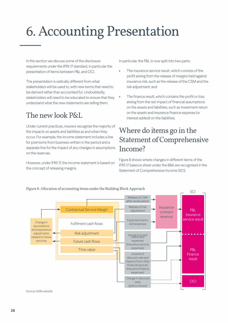
In particular, the P&L is now split into two parts:

• The insurance service result, which consists of the profit arising from the release of margins held against insurance risk, such as the release of the CSM and the risk adjustment; and

• The finance result, which contains the profit or loss arising from the net impact of financial assumptions on the assets and liabilities, such as investment return on the assets and insurance finance expense (or interest added) on the liabilities.

Where do items go in the Statement of Comprehensive Income?Figure 8 shows where changes in different items of the IFRS 17 balance sheet under the BBA are recognised in the Statement of Comprehensive Income (SCI).

6. Accounting Presentation

Figure 8. Allocation of accounting items under the Building Block Approach

Change in assumptions

and experience adjustments

related to future services

Source: IASB website

Fulfilment cash flows

Risk adjustment

Future cash flows

Time value

Change in discount rates

(policy choice)

Insurance contract revenue

OCI

Contractual Service Margin

Actual incurred claims and expenses

(Insurance service expenses)

Unwind of discount rate and

impacts from other financial sources

(insurance finance expenses)

Release of CSM after recalculation

Expected claims and expenses

Release of risk adjustment P&L

Insurance service result

P&L Finance

result

SCI

24

This presentation poses three key challenges or choices to insurers.

1. Removal of investment components from revenue

As a result of the disaggregation between insurance and finance results, any investment component under the BBA that has not been unbundled (because it is highly interrelated to the insurance component) should be excluded from insurance contract revenue within the insurance service result.

An investment component is defined as the amount the insurer has to pay regardless of whether the insured event happens. This amount implicitly belongs to the policyholder and therefore should not be included as revenue. This includes any amounts paid at maturity or surrender, as well as the amount of cash surrender value that is implicit in the amounts paid when the insured event happens.

The main complexity with separating out investment components is that many accounting systems currently do not record this information and values are only calculated if a policyholder surrenders before death. There may be additional complexity if the insurer is able to exercise discretion over the amounts paid. Our endowment assurance example in the Appendix sheds more light on how investment components, which can’t be unbundled, are separated.

2. Deciding where to report discount rate changes

Insurers can choose to report changes in discount rates on the BEL and RA in either P&L (as part of insurance finance expense) or OCI. The policy choice gives insurers an option to choose the most appropriate policy for each of their portfolios, depending on the relative cost/benefit of:

• Reporting changes in P&L to reduce accounting mismatches, which is driven by where changes in the value of financial assets are recognised, or

• Reporting changes in OCI to reflect the long-term nature of the contract by excluding short-term market fluctuations from the P&L.

Insurers can also make a similar choice for contracts measured under the VFA approach and present all insurance finance expenses in the P&L or disaggregate amounts between the P&L and OCI if this reduces accounting mismatches.

3. Disaggregation of the release of the risk adjustment

Given the different methods that can be used to measure the risk adjustment, IFRS 17 does not require insurers to disaggregate the release of the risk adjustment into an insurance service result and a finance result. The entire change can be presented as part of the insurance contract revenue within the insurance service result.

However, insurers are permitted to disaggregate the release if they wish, and present the insurance finance expenses on the risk adjustment in a way that is consistent with their accounting policy choice.

25

Figure 9. Reconciliation of insurance contract revenue

Margins released xRelease of CSM xRelease of risk adjustment xAmortisation of directly attributable acquisition costs x

Total margins released xClaims and expenses x

Actual claims xActual expenses x

Total claims and expenses xExperience adjustments – claims xExperience adjustments – expenses xTotal insurance contract revenue x

Source: IASB website

Reconciliation of revenue Insurers will also have to include in their disclosures a reconciliation of the items that form the insurance contract revenue in the P&L, an example of which is shown in figure 9 below. A numerical example is also included in the Appendix of this paper.

Other disclosure requirementsThe Statement of Comprehensive Income and the reconciliation of contract revenue are just two of the disclosure requirements under IFRS 17. The full list is far bigger, containing both qualitative and quantitative disclosures. It also comes with the added complexity of having to aggregate or disaggregate information so that useful information is not obscured by a large amount of insignificant detail or by the aggregation of items that have different characteristics. For example, insurers will need to disaggregate information for insurance contracts issued and reinsurance contracts.

It is questionable whether the level of detail required in the disclosures will increase the clarity of the business for investors or actually add complication. We do not set all of the detail in this paper, but it can be accessed readily in the IFRS 17 standard document.

26

GlossaryAccrete interestAdd on interest

BBA Building Block Approach

BEL Best Estimate Liabilities

Building Block Approach Also called the general model. It is the main measurement model under IFRS 17.

Contract boundaries The point at which insurance coverage ends for the inforce contract and the issuer has the right to revalue the benefits or reassess the price of the contract.

Contractual service margin The amount of liability held on top of the best estimate liability and risk adjustment to eliminate any day one profits.

Coverage units The amount of coverage/service provided by the contracts in the group, determined by considering the amount of benefits provided and the expected duration of the contract.

Coverage units can be for example the number of policies in-force each period or the expected benefits paid each period.

Coverage period The term of the contract.

CSM Contractual Service Margin.

Experience adjustment The impact arising from actual experience being different from expected experience over the reporting period.

Finance result The amount of profit arising from a portfolio of contracts from financial or economic sources, such as the interest added on the liabilities or the investment return from the assets

Fulfilment cash flows Present value of the future cash flows plus the risk adjustment for non-financial risk.

Insurance component This is the component of the contract which represents the service provided in relation to insurance risk.

IASB International Accounting Standards Board

Insurance finance expenses This is the part of the finance result arising from the liability side

Insurance service expenses This comprises of incurred claims (excluding repayments of investment components), other incurred expenses, amortisation of acquisition costs, changes to liability amounts that relate to past service and changes that relate to future service.

Insurance service result This is the amount of profit arising from non-financial related risks. It can also be thought of as the underwriting profit.

Investment component The amounts that the insurer has to pay the policyholder of a contract even if the insured event does not occur.

Loss component The amount of loss from onerous contracts that is held separately on the balance sheet and does not form part of the insurance revenue.

Onerous contract A contract that is expected to make an overall loss. The CSM for an onerous contract is zero.

Directly participating contracts Contracts which satisfy each of the following requirements:

• The contract terms specify a clearly identified pool of underlying items in which the policyholder participates

• The insurer is expected to pay policyholders a substantial share of the fair value returns on those items

• The insurer expects a substantial proportion of the change in amounts paid to the policyholder to vary with the change in the fair value of the underlying items.

OCI Statement of Other Comprehensive Income

PAA Premium Allocation Approach

P&L Statement of Profit or Loss

Premium Allocation Approach A permitted simplification to the building block approach provided the measurement results in a good enough approximation. This approach is generally used for contracts with durations of one year or less.

RA Risk Adjustment

Risk adjustment The amount insurers require for bearing the uncertainty about the amount and timing of the cash flows that arises from non-financial risks.

Underlying items The pool of items which determine the amounts payable to the policyholder of a directly participating contract. An example can be a pool of financial assets.

Unlocking the CSM Updating the CSM for change in assumptions.

Variable Fee Approach The measurement model used for directly participating contracts.

VFA Variable Fee Approach 27

The following section illustrates the treatment under IFRS 17 for various types of insurance products. A simplified case study on conventional non-profit annuities is set out in detail. We then provide a further three examples for a non-profit endowment assurance product, a property-linked product and a reinsurance contract held.

Please note that the profit and loss statements we’ve presented do not group actual claims incurred and expenses incurred into insurance service expense, which is the terminology and presentation used in the official examples provided by the IASB as part of the standard. This is for clarity to enable numbers to be tracked. Furthermore, numbers may not tie exactly to manual calculation as a result of rounding.

Non-profit annuity exampleAssumptionsAn insurer issues a portfolio of conventional non-profit annuity contracts. The following have been assumed for measurement purposes:

• The coverage is expected to be 10 years.

• A premium is only paid at contract inception of the value £270,000.

• Directly attributable acquisition costs of £10,000 are incurred at contract inception, which are spread over the coverage period in line with BEL, with an allowance for time value.

• The insurer incurs annual maintenance expenses with initial value of £1,000, which escalates with inflation at each subsequent year.

• The risk adjustment is calculated using the cost of capital approach, similar to that used in Solvency II.

• The CSM is run down in line with the BEL.

The one year forward discount curves at inception (t=0), and at the end of year 1 and 2 (t=1 and t=2 respectively) and the forward inflation curve are shown in figure 10. Numbers have been rounded to two decimal places. The forward inflation rate is assumed unchanged for each period. For ease of reconciliation for the reader we also include below the calculated discount factors corresponding to the discount rates.

Figure 10. Discount rate and inflation rate assumptions

Discount rates Discount Factors Inflation Rate

Year t=0 t=1 t=2 Year t=0 t=1 t=2 Year t=0,1,2

0 0 1 0 1 1.73% 1 0.9830 1 1 2.54%2 2.23% 2.13% 2 0.9616 0.9791 1 2 2.57%3 2.62% 2.52% 2.42% 3 0.9370 0.9551 0.9764 3 2.96%4 2.82% 2.72% 2.62% 4 0.9113 0.9297 0.9514 4 2.67%5 3.02% 2.92% 2.82% 5 0.8846 0.9034 0.9254 5 2.67%6 3.17% 3.07% 2.97% 6 0.8574 0.8765 0.8986 6 2.72%7 3.32% 3.22% 3.12% 7 0.8299 0.8491 0.8714 7 2.81%8 3.37% 3.27% 3.17% 8 0.8028 0.8223 0.8447 8 2.93%9 3.46% 3.36% 3.26% 9 0.7760 0.7955 0.8180 9 3.07%10 3.45% 3.35% 3.25% 10 0.7501 0.7698 0.7923 10 3.20%

Appendix – Case studies

Worked examplesThis part of the paper sets out some simplified worked examples of the standard in practice

28

The cash flows at initial recognition related to this portfolio of contracts is indicated in figure 11. Acquisition costs are amortised at the same rate as the BEL and an allowance is made for time value. This results in implied cash flows as shown in figure 11 below.

Figure 11. Cash flow projections at initial recognition

Year 0 1 2 3 4 5 6 7 8 9 10

Premium received (270,000)Cash outflows 44,359 38,836 33,431 28,241 23,360 18,872 14,848 11,339 8,372 5,950Cash inflows - - - - - - - - - -Acquisition costs - 2,140 1,874 1,613 1,363 1,127 911 716 547 404 287Expenses - 1,025 1,052 1,083 1,112 1,141 1,173 1,206 1,241 1,279 1,320Cost of Capital 3,767 3,025 2,387 1,842 1,381 998 686 439 248 105 -

This example will step through the impact of changes in discount rates through the first accounting period (t=1) and the impact of three different cumulative changes through the second accounting period (t=2), as detailed in the diagram below.

Initial measurement Discount rates

Scenario a) Experience variance Scenario b) Future assumption change

Scenario c) Discount rates

Impact of experience variance on incurred claims recognised immediately

in P&L. Impact of experience variance on future cash flows and future

assumption change adjusts the CSM, calculated using t=0 rates.

BEL and risk adjustment are updated to reflect the change in discount rates. The CSM is not impacted by the assumption

change, resulting in the same closing balance as expected.

Assumption change

Subsequent Measurement t=1

Subsequent Measurement t=2

Measurement summary

A

B C

A: Initial measurement of contracts at inceptionFigure 12 shows how the CSM is calculated at initial recognition based on the cash flows in figure 11.

Figure 12. Liability measurement at initial recognition

£ Notes

(a) Premium (270,000)

(b) Present value of cash outflows 207,244 Discounted using discount rate t=0

(c) Present value of cash inflows -

(d) Directly attributable acquisition costs 10,000 Discounted using discount rate t=0

(e) Present value of expenses 10,041 Discounted using discount rate t=0

(f) Total present value of future cash flows 227,286 (b)+(c)+(d)+(e)

(g) Risk adjustment 14,137 Discounted using discount rate t=0

(h) Total fulfilment cash flows 241,423 (f)+(g)

(i) Contractual service margin 28,577 - (a) - (h)

29

IFRS 17 requires the CSM to be recognised on a basis which reflects the transfer of services. In our example, we have chosen to run-off the CSM in line with the present value of future cash flows (BEL), resulting in the run-off pattern shown in figure 13. As the CSM is run-down from period to period, an element of this will reflect time value changes, which ultimately feeds through as interest accreted and forms part of the insurance finance expense. We have split this out in figure 13 as this does not form part of the insurance service result (or underwriting profit). For example at time 1, the CSM of £28,577 increases with interest of 1.73% before it is allocated to the period, resulting in an allocated amount of £5,975 as the balancing item to get to the CSM value of £23,095 at time 2.

Equivalently, the starting value of liabilities can be updated for interest (i.e. £227,286 x 1.0173 = £231,206) and the ratio of this liability value and that at time 2 is then used to run-down the adjusted CSM (i.e. (£183,682 / £231,206– 1) x (28,577 x 1.0173) = -5,975). This effectively means that the allocation of the CSM is based on the change in cash flows in the period (i.e. the service provided by the book of contracts).

Figure 13. Expected run-off of the CSM and contribution to profit

Liability run-off Contribution of profit over the year

A B C D E F

Time BEL run-off Run-off of CSM Year Total profit from CSM

Interest accreted / unwind of discount rate

Allocation of CSM

(underwriting profit)

(Same row ratios as column B)

(Difference in row values in

column C)

(Previous row value in column C multiplied by

corresponding forward IR)(Column D -

column E)

0 227,286 28,5771 183,682 23,095 1 5,482 (493) 5,9752 146,019 18,359 2 4,735 (515) 5,2513 113,715 14,298 3 4,062 (481) 4,5424 86,212 10,840 4 3,458 (404) 3,8625 63,184 7,944 5 2,895 (327) 3,2226 44,234 5,562 6 2,383 (252) 2,6357 28,933 3,638 7 1,924 (185) 2,1098 16,780 2,110 8 1,528 (122) 1,6509 7,305 918 9 1,191 (73) 1,26410 - - 10 918 (32) 950

The allocation of the CSM each period after allowing for interest is the expected unearned profit recognised from the margin each year. This and the release in the risk adjustment is the total expected underwriting profit or insurance service result from the contract (assuming that the release of the risk adjustment is not disaggregated between an underwriting and finance component).

30

B: Subsequent measurement at time 1We assume at time 1 that the actual cash flows for the period are the same as that projected at inception and the projection of future cash flows beyond time 1 is also unchanged. The only assumption change is the discount rate, which moves in accordance with figure 10. The projected cash flows are unchanged from figure 11, but the cost of capital projections change as a result of the methodology used. The projections and resulting liability measurement are shown in figure 14a.

Figure 14a. Cash flows at time 1

Assumption date

Cash flow Discounted value @ t=1

1 2 3 4 5 6 7 8 9 10

t=0 Cash outflows 166,460 38,836 33,431 28,241 23,360 18,872 14,848 11,339 8,372 5,950

Acquisition costs 8,032 1,874 1,613 1,363 1,127 911 716 547 404 287

Expenses 9,189 1,052 1,083 1,112 1,141 1,173 1,206 1,241 1,279 1,320

Total BEL 183,682

Cost of Capital 10,549 3,025 2,387 1,842 1,381 998 686 439 248 105 -

t=1 Cash outflows 167,027 38,836 33,431 28,241 23,360 18,872 14,848 11,339 8,372 5,950

Acquisition costs 8,059 1,874 1,613 1,363 1,127 911 716 547 404 287

Expenses 9,234 1,052 1,083 1,112 1,141 1,173 1,206 1,241 1,279 1,320

Total BEL 184,320

Cost of Capital 10,600 3,036 2,395 1,847 1,384 1,000 688 440 248 105 -

Figure 14b. Changes in present values at time 1

Cash flow Discounted value @ t=1

Cash outflows 567

Acquisition costs 27

Expenses 45

Total BEL 639

Risk Adjustment 50

Discounted values are calculated using the discount rates in force at the assumption date. The differences between the present values of the cash outflows, acquisition costs and expenses between the two rows reflect the impact of changes in discount rates. The difference between the discounted values of the costs of capital reflects both the impact of changes in discount rates and differences in the costs of capital.

The change in discount rates will affect the run-off of the BEL, but the run-off pattern of the CSM is still based on inception discount rates and thus remains unchanged. Since the actual and projected cash flows are unchanged from inception, the CSM at time 1 is the same as that expected, in line with figure 13.

Figure 15a to 15c below is a reconciliation of the CSM, the present value of future cash flows and the risk adjustment. Note that IFRS 17 requires the disclosure of a reconciliation of the total contract liabilities to be split between the liability for remaining coverage, excluding the loss component; the loss component of the liability for remaining coverage; and the liability for incurred claims. We have not provided this disclosure in our example as this is essentially a reallocation of each of the items provided in the reconciliations in 15a to 15c. Please refer to the examples from the IASB for the disclosure mentioned.

31

Figure 15a: Reconciliation of CSM at time 1

Reconciliation of CSM £ Notes

(a^) Opening balance 28,577 See (i) in figure 12(b^) Interest accreted (t=0 rates) 493 Opening balance x Interest for t=1 at t=0(c^) Experience adjustment - incurred claims -(d^) Experience adjustment – Present value of future cash flows -(e^) Experience adjustment - risk adjustment -(f^) Changes in non-economic assumptions

– Present value of future Cash flows-

(g^) Changes in non-economic assumptions - risk adjustment -(h^) Amount recognised with service (5,975) See column F in figure 13(i^) Closing balance 23,095 Sum of above

The impact of the change in discount rates does not adjust the CSM and flows directly into P&L or OCI depending on the insurer’s accounting policy. As a result the closing balance of the CSM is unchanged from that projected and thus the value of £23,095 coincides with the second row of column C in figure 13.

Figure 15b. Reconciliation of BEL at time 1

Reconciliation of BEL (incl. expenses) £ Notes

(j^) Opening balance 227,286 See (f) in figure 12(k^) Interest accreted (t=0 rates)

3,921Opening balance x Interest for t=1 at t=0.

227,286 x 1.73%(l^) Experience adjustment - incurred claims -(m^) Experience adjustment – Present value of future cash

flows-

(n^) Changes in non-economic assumptions

– Present value of future cash flows-

(o^) Amount recognised with service (47,525) Sum of CFs at t=1. See figure 11(p^) Claims paid (44,359) See figure 11(q^) Amortisation of acquisition costs (2,140) See figure 11(r^) Maintenance expenses paid (1,025) See figure 11(s^) Change in discount curve 639 See figure 14b.(t^) Balance carried forward 184,320 Sum of above

Interest on BEL is calculated on start-of-period rates. The amount recognised with service is the sum of all actual cash flows incurred in the period. Unlike the CSM, the BEL should reflect current market discount rates, hence the impact of discount rate changes feeds into the reconciliation.

Figure 15c: Reconciliation of risk adjustment

Reconciliation of risk adjustment £ Notes

(u^) Opening balance 14,137 See (g) in figure 12(v^) Experience adjustment – Present value of future cash flows -(w^) Changes in non-economic assumptions – Present value of

future cash flows-

(x^) Amount recognised with service (3,588) Run-off of risk adjustment(y^) Change in discount curve

50Difference in PV of CoC items from figure

14b(z^) Balance carried forward 10,600

In this example, we have not disaggregated the run-off of the risk adjustment between unwind of the discount rate and the amount recognised with service – the sum of these are presented as one.

32

Figure 16 below shows some of the financial statements expected to be disclosed for year 1.

Figure 16. Disclosure requirements

Calculation of insurance contract revenue Year 1 Notes

Margins released Contractual service margin 5,975 = - (h )̂ in figure 15a Directly attributable acquisition costs 2,140 = - (q )̂ in figure 15b Risk adjustment 3,588 = - (x )̂ in figure 15c Total margins released 11,704 Claims and expenses Actual claims 44,359 = - (p )̂ in figure 15b Actual expenses 1,025 = - (r )̂ in figure 15b Total actual claims and expenses 45,384 Experience variance - Claims 0 Zero as this example has no experience adjustments Total insurance contract revenue 57,088

Analysis of insurance finance expense in profit or loss / total comprehensive income Year 1 Notes

Interest accretion at start of period rate 4,414 = (b )̂ in figure 15a + (k )̂ in figure 15bDifference between the measurement of amounts that adjust the CSM at locked-in and start of period rate

- Zero as no assumption changes which modify the CSM in this example

Effect of change in discount rates in period 689 = (s )̂ in figure 15b + (y )̂ in figure 15cTotal insurance finance expenses in period 5,103 If the OCI approach is used, this will also need to be split into: (Profit or loss) Insurance finance expense 4,414 = (b )̂ in figure 15a + (k )̂ in figure 15bMovement in OCI 689 Balancing item Total insurance finance expenses in period 5,103

Statement of profit and loss and other comprehensive income Year 1 Notes

Insurance contract revenue 57,088 See calculation of contract revenue in figure 16Incurred claims (44,359) = (p )̂ in figure 15bIncurred expenses (1,025) = (r )̂ in figure 15bAmortisation of directly attributable acquisition costs (2,140) = (q )̂ in figure 15bAmounts which do not adjust the contractual service margin -Insurance service result 9,563Investment income x See note (1)Insurance finance expenses (4,414) = - (b )̂ in figure 15a - (k )̂ in figure 15bProfit before tax 5,150Gains or losses on financial assets measured at fair value through OCI x See note (1)Effect of discount rate changes on insurance liability (optional) (689) = - (s )̂ in figure 15b - (y )̂ in figure 15cTotal comprehensive income 4,461

Note (1) Values should be measured in accordance with the appropriate IFRS (e.g. IFRS 9 for financial assets). We have set these to zero in the example, but realistically these items will be non-zero and total profit before tax would be higher.

33

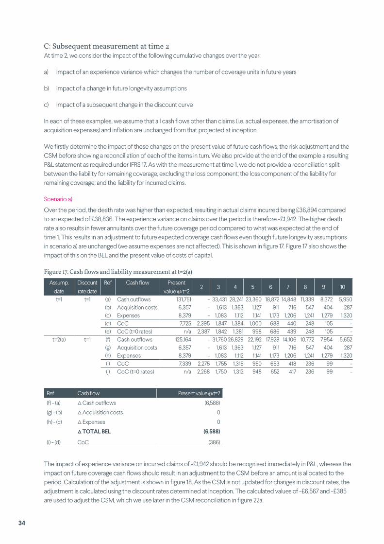
C: Subsequent measurement at time 2At time 2, we consider the impact of the following cumulative changes over the year:

a) Impact of an experience variance which changes the number of coverage units in future years

b) Impact of a change in future longevity assumptions

c) Impact of a subsequent change in the discount curve

In each of these examples, we assume that all cash flows other than claims (i.e. actual expenses, the amortisation of acquisition expenses) and inflation are unchanged from that projected at inception.

We firstly determine the impact of these changes on the present value of future cash flows, the risk adjustment and the CSM before showing a reconciliation of each of the items in turn. We also provide at the end of the example a resulting P&L statement as required under IFRS 17. As with the measurement at time 1, we do not provide a reconciliation split between the liability for remaining coverage, excluding the loss component; the loss component of the liability for remaining coverage; and the liability for incurred claims.

Scenario a)

Over the period, the death rate was higher than expected, resulting in actual claims incurred being £36,894 compared to an expected of £38,836. The experience variance on claims over the period is therefore -£1,942. The higher death rate also results in fewer annuitants over the future coverage period compared to what was expected at the end of time 1. This results in an adjustment to future expected coverage cash flows even though future longevity assumptions in scenario a) are unchanged (we assume expenses are not affected). This is shown in figure 17. Figure 17 also shows the impact of this on the BEL and the present value of costs of capital.

Figure 17. Cash flows and liability measurement at t=2(a)Assump.

dateDiscount rate date

Ref Cash flow Present value @ t=2

2 3 4 5 6 7 8 9 10

t=1 t=1 (a) Cash outflows 131,751 - 33,431 28,241 23,360 18,872 14,848 11,339 8,372 5,950(b) Acquisition costs 6,357 - 1,613 1,363 1,127 911 716 547 404 287(c) Expenses 8,379 - 1,083 1,112 1,141 1,173 1,206 1,241 1,279 1,320(d) CoC 7,725 2,395 1,847 1,384 1,000 688 440 248 105 -(e) CoC (t=0 rates) n/a 2,387 1,842 1,381 998 686 439 248 105 -

t=2(a) t=1 (f) Cash outflows 125,164 - 31,760 26,829 22,192 17,928 14,106 10,772 7,954 5,652(g) Acquisition costs 6,357 - 1,613 1,363 1,127 911 716 547 404 287(h) Expenses 8,379 - 1,083 1,112 1,141 1,173 1,206 1,241 1,279 1,320(i) CoC 7,339 2,275 1,755 1,315 950 653 418 236 99 -(j) CoC (t=0 rates) n/a 2,268 1,750 1,312 948 652 417 236 99 -

Ref Cash flow Present value @ t=2

(f) - (a) ∆ Cash outflows (6,588)

(g) - (b) ∆ Acquisition costs 0

(h) - (c) ∆ Expenses 0

∆ TOTAL BEL (6,588)

(i) - (d) CoC (386)

The impact of experience variance on incurred claims of -£1,942 should be recognised immediately in P&L, whereas the impact on future coverage cash flows should result in an adjustment to the CSM before an amount is allocated to the period. Calculation of the adjustment is shown in figure 18. As the CSM is not updated for changes in discount rates, the adjustment is calculated using the discount rates determined at inception. The calculated values of -£6,567 and -£385 are used to adjust the CSM, which we use later in the CSM reconciliation in figure 22a.

34

Figure 18. Calculation of CSM adjustment under scenario a)Assump.

dateDiscount rate date Ref

Cash flow Present value @

t=22 3 4 5 6 7 8 9 10

t=2(a)

minus

t=1

t=0 (a*) ∆ Cash outflows (6,567) 0 (1,672) (1,412) (1,168) (944) (742) (567) (419) (297)(b*) ∆ Acquisition costs 0 0 0 0 0 0 0 0 0 0(c*) ∆ Expenses 0 0 0 0 0 0 0 0 0 0(d*) ∆ CoC (t=0) (385) (119) (92) (69) (50) (34) (22) (12) (5) 0

Scenario b)

We now consider the impact of a weakening in the future longevity trend assumption, which reduces the future projected coverage cash flows further. We again assume that expected expenses and discount rates are unchanged from those at time 1 under this scenario. The revised expected cash flows are shown in figure 19.

Figure 19. Cash flows and liability measurement at t=2(b)Assump.

dateDiscount rate date

Ref Cash flow Present value @ t=2

2 3 4 5 6 7 8 9 10

t=2(a) t=1 (f) Cash outflows 125,164 - 31,760 26,829 22,192 17,928 14,106 10,772 7,954 5,652(g) Acquisition costs 6,357 - 1,613 1,363 1,127 911 716 547 404 287(h) Expenses 8,379 - 1,083 1,112 1,141 1,173 1,206 1,241 1,279 1,320(i) CoC 7,339 2,275 1,755 1,315 950 653 418 236 99 -(j) CoC (t=0 rates) - 2,268 1,750 1,312 948 652 417 236 99 -

t=2(b) t=1 (k) Cash outflows 124,636 - 31,696 26,748 22,103 17,839 14,021 10,697 7,890 5,602(l) Acquisition costs 6,357 - 1,613 1,363 1,127 911 716 547 404 287

(m) Expenses 8,379 - 1,083 1,112 1,141 1,173 1,206 1,241 1,279 1,320(n) CoC 6,772 2,102 1,620 1,213 876 602 385 217 91 -(o) CoC (t=0 rates) - 2,096 1,616 1,210 874 601 384 217 91 -

Ref Cash flow Present value @ t=2

(k) - (f) ∆ Cash outflows (528)

(l) - (g) ∆ Acquisition costs 0

(m) - (h) ∆ Expenses 0

∆ TOTAL BEL (528)

(n) - (i) CoC (566)

Like scenario a) the CSM is adjusted to allow for the impact from the assumption change. The adjustment is based on inception discount rates and shown in figure 20. The calculated values of -£526 and -£563 are used to adjust the CSM, which we use later in the CSM reconciliation in figure 22a.

Figure 20. Calculation of CSM adjustment under scenario b)Assump.

dateDiscount rate date

Ref Cash flow Present value @ t=2

2 3 4 5 6 7 8 9 10

t=2(b)

minus

t=2(a)

t=0 (e*)

(f*)

(g*)

(h*)

∆ Cash outflows (526) 0 (63) (80) (89) (89) (84) (75) (63) (51)∆ Acquisition costs 0 0 0 0 0 0 0 0 0 0∆ Expenses 0 0 0 0 0 0 0 0 0 0∆ CoC (t=0 rates) (563) (172) (134) (101) (74) (51) (33) (19) (8) 0

35

Scenario c)

Noting that discount rates had already changed at t=1, we now look at the impact of a subsequent interest rate change at t=2. Figure 21 shows the resulting changes in present value on each of the fulfilment cash flows. The impact does not adjust the CSM and feeds straight through into P&L.

Figure 21. Cash flows and liability measurement at t=2(c)Assump.

dateDiscount rate date

Ref Cash flow Present value @ t=2

2 3 4 5 6 7 8 9 10

t=2(b) t=1 (k) Cash outflows 124,636 - 31,696 26,748 22,103 17,839 14,021 10,697 7,890 5,602(l) Acquisition costs 6,357 - 1,613 1,363 1,127 911 716 547 404 287(m) Expenses 8,379 - 1,083 1,112 1,141 1,173 1,206 1,241 1,279 1,320(n) Cost of Capital 6,772 2,102 1,620 1,213 876 602 385 217 91 -

t=2(c) t=2(c) (p) Cash outflows 125,027 - 31,696 26,748 22,103 17,839 14,021 10,697 7,890 5,602(q) Acquisition costs 6,377 - 1,613 1,363 1,127 911 716 547 404 287(r) Expenses 8,416 - 1,083 1,112 1,141 1,173 1,206 1,241 1,279 1,320(s) Cost of Capital 6,801 2,108 1,625 1,216 878 603 386 217 91 -

Reconciliation of BEL, risk adjustment and CSM

Figure 22a shows a reconciliation of the CSM at time 2 based on the adjustments calculated in figure 18 and figure 20 above. The CSM is adjusted against all changes to the present value of future cash flows, which are not caused by changes in economic assumptions. Please note that where the impact on BEL is negative, the adjustment to the CSM is positive to offset this impact. For example the impact of -£6,567 in figure 18 results in an impact of +£6,567 on the CSM. Incurred claims do not adjust the CSM and will feed through directly into P&L.

Figure 22a. Reconciliation of CSM Ref Reconciliation of CSM £ Notes

(a±) Opening balance 23,095 See (i )̂ figure 15a(b±) Interest accreted (t=0 rates) 515 Opening balance x interest at t=2 as at t=0

23,095 x 2.23%(c±) Experience adjustment - incurred claims -(d±) Experience adjustment – Present value of future cash flows 6,567 - (a*) in figure 18(e±) Experience adjustment - risk adjustment 385 - (d*) in figure 18(f±) Changes in non-economic assumptions – Present value of

future cash flows526 - (e*) in figure 20

(g±) Changes in non-economic assumptions - risk adjustment 563 - (h*) in figure 20(h±) Amount recognised with service (7,051) As detailed below

(i±) Closing balance 24,600

We now explain how we calculate the value (h±) in figure 22a. In our example, we’re basing the CSM run-off on the pattern of run-off of the BEL. As a result, this pattern is updated for changes in non-financial assumptions and experience adjustments. However, it is not updated for changes in financial assumptions. Figure 22b shows how the BEL at time 2, based on inception rates, is adjusted for the assumption changes. This value is used to allocate the CSM as shown in figure 22c.

Figure 22b. Reconciliation of the BEL at time 2 on inception ratesReconciliation of BEL at time 2 on inception rates £ Notes

Value of BEL before assumption changes 146,019 See row 3, column B of figure 13Impact from experience adjustments in scenario (a) (6,567) See (a*) from figure 18Impact from non-financial assumption changes in scenario (b) (526) See (e*) from figure 20Value of BEL after assumption changes 138,926

36

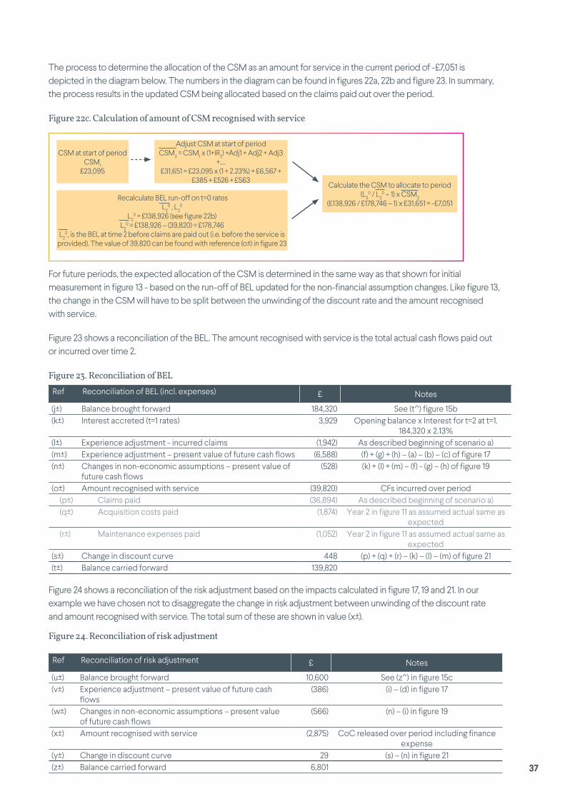
The process to determine the allocation of the CSM as an amount for service in the current period of -£7,051 is depicted in the diagram below. The numbers in the diagram can be found in figures 22a, 22b and figure 23. In summary, the process results in the updated CSM being allocated based on the claims paid out over the period.

Figure 22c. Calculation of amount of CSM recognised with service

For future periods, the expected allocation of the CSM is determined in the same way as that shown for initial measurement in figure 13 - based on the run-off of BEL updated for the non-financial assumption changes. Like figure 13, the change in the CSM will have to be split between the unwinding of the discount rate and the amount recognised with service.

Figure 23 shows a reconciliation of the BEL. The amount recognised with service is the total actual cash flows paid out or incurred over time 2.

Figure 23. Reconciliation of BELRef Reconciliation of BEL (incl. expenses) £ Notes

(j±) Balance brought forward 184,320 See (t^) figure 15b(k±) Interest accreted (t=1 rates) 3,929 Opening balance x Interest for t=2 at t=1.

184,320 x 2.13%(l±) Experience adjustment - incurred claims (1,942) As described beginning of scenario a)(m±) Experience adjustment – present value of future cash flows (6,588) (f) + (g) + (h) – (a) – (b) – (c) of figure 17(n±) Changes in non-economic assumptions – present value of

future cash flows(528) (k) + (l) + (m) – (f) - (g) – (h) of figure 19

(o±) Amount recognised with service (39,820) CFs incurred over period(p±) Claims paid (36,894) As described beginning of scenario a)(q±) Acquisition costs paid (1,874) Year 2 in figure 11 as assumed actual same as

expected(r±) Maintenance expenses paid (1,052) Year 2 in figure 11 as assumed actual same as

expected(s±) Change in discount curve 448 (p) + (q) + (r) – (k) – (l) – (m) of figure 21(t±) Balance carried forward 139,820

Figure 24 shows a reconciliation of the risk adjustment based on the impacts calculated in figure 17, 19 and 21. In our example we have chosen not to disaggregate the change in risk adjustment between unwinding of the discount rate and amount recognised with service. The total sum of these are shown in value (x±).

Figure 24. Reconciliation of risk adjustment

Ref Reconciliation of risk adjustment £ Notes

(u±) Balance brought forward 10,600 See (z^) in figure 15c(v±) Experience adjustment – present value of future cash

flows(386) (i) – (d) in figure 17

(w±) Changes in non-economic assumptions – present value of future cash flows

(566) (n) – (i) in figure 19

(x±) Amount recognised with service (2,875) CoC released over period including finance expense

(y±) Change in discount curve 29 (s) – (n) in figure 21(z±) Balance carried forward 6,801

CSM at start of period CSM1

£23,095

Adjust CSM at start of period CSM2 = CSM1 x (1+IR2) +Adj1 + Adj2 + Adj3

+…. £31,651 = £23,095 x (1 + 2.23%) + £6,567 +

£385 + £526 + £563

Recalculate BEL run-off on t=0 rates L2

0 , L20

L20 = £138,926 (see figure 22b)

L20 = £138,926 – (39,820) = £178,746

L20, is the BEL at time 2 before claims are paid out (i.e. before the service is

provided). The value of 39,820 can be found with reference (o±) in figure 23

Calculate the CSM to allocate to period (L2

0 / L20 – 1) x CSM2

(£138,926 / £178,746 – 1) x £31,651 = -£7,051

37

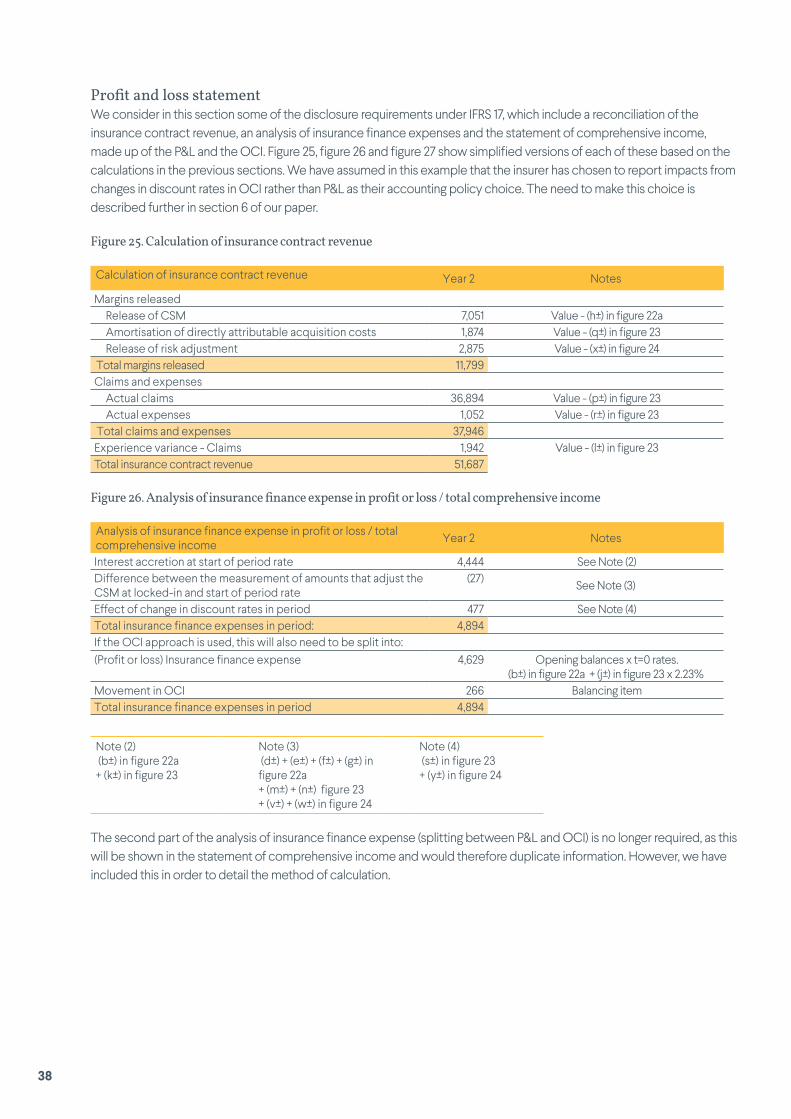
Profit and loss statement We consider in this section some of the disclosure requirements under IFRS 17, which include a reconciliation of the insurance contract revenue, an analysis of insurance finance expenses and the statement of comprehensive income, made up of the P&L and the OCI. Figure 25, figure 26 and figure 27 show simplified versions of each of these based on the calculations in the previous sections. We have assumed in this example that the insurer has chosen to report impacts from changes in discount rates in OCI rather than P&L as their accounting policy choice. The need to make this choice is described further in section 6 of our paper.

Figure 25. Calculation of insurance contract revenue

Calculation of insurance contract revenue Year 2 Notes

Margins released Release of CSM 7,051 Value - (h±) in figure 22a Amortisation of directly attributable acquisition costs 1,874 Value - (q±) in figure 23 Release of risk adjustment 2,875 Value - (x±) in figure 24 Total margins released 11,799 Claims and expenses Actual claims 36,894 Value - (p±) in figure 23 Actual expenses 1,052 Value - (r±) in figure 23 Total claims and expenses 37,946 Experience variance - Claims 1,942 Value - (l±) in figure 23Total insurance contract revenue 51,687

Figure 26. Analysis of insurance finance expense in profit or loss / total comprehensive income

Analysis of insurance finance expense in profit or loss / total comprehensive income Year 2 Notes

Interest accretion at start of period rate 4,444 See Note (2)Difference between the measurement of amounts that adjust the CSM at locked-in and start of period rate

(27) See Note (3)

Effect of change in discount rates in period 477 See Note (4)Total insurance finance expenses in period: 4,894 If the OCI approach is used, this will also need to be split into:(Profit or loss) Insurance finance expense 4,629 Opening balances x t=0 rates.

(b±) in figure 22a + (j±) in figure 23 x 2.23% Movement in OCI 266 Balancing item Total insurance finance expenses in period 4,894

Note (2) (b±) in figure 22a + (k±) in figure 23

Note (3) (d±) + (e±) + (f±) + (g±) in figure 22a + (m±) + (n±) figure 23 + (v±) + (w±) in figure 24

Note (4) (s±) in figure 23+ (y±) in figure 24

The second part of the analysis of insurance finance expense (splitting between P&L and OCI) is no longer required, as this will be shown in the statement of comprehensive income and would therefore duplicate information. However, we have included this in order to detail the method of calculation.

38

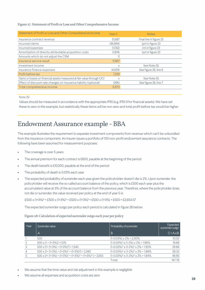
Figure 27. Statement of Profit or Loss and Other Comprehensive Income

Statement of Profit or Loss and Other Comprehensive Income Year 2 Notes

Insurance contract revenue 51,687 Final line in figure 25Incurred claims (36,894) (p±) in figure 23Incurred expenses (1,052) (r±) in figure 23Amortisation of directly attributable acquisition costs (1,874) (q±) in figure 23Amounts which do not adjust the CSM 0Insurance service result 11,867Investment income x See Note (5)Insurance finance expenses (4,629) See figure 26, line 6Profit before tax 7,239Gains or losses on financial assets measured at fair value through OCI x See Note (5)Effect of discount rate changes on insurance liability (optional) (266) See figure 26, line 7Total comprehensive income 6,973

Note (5)

Values should be measured in accordance with the appropriate IFRS (e.g. IFRS 9 for financial assets). We have set these to zero in the example, but realistically these items will be non-zero and total profit before tax would be higher.

Endowment Assurance example - BBAThis example illustrates the requirement to separate investment components from revenue which can’t be unbundled from the insurance component. An insurer issues a portfolio of 100 non-profit endowment assurance contracts. The following have been assumed for measurement purposes:

• The coverage is over 5 years

• The annual premium for each contract is £600, payable at the beginning of the period

• The death benefit is £10,000, payable at the end of the period

• The probability of death is 0.03% each year

• The expected probability of surrender each year given the policyholder doesn’t die is 2%. Upon surrender, the policyholder will receive the so called account balance of the policy, which is £500 each year plus the accumulated value at 3% of the account balance from the previous year. Therefore, where the policyholder does not die or surrender, the value received per policy at the end of year 5 is:

£500 x (1+3%)4 + £500 x (1+3%)3 + £500 x (1+3%)2 + £500 x (1+3%) + £500 = £2,654.57

The expected surrender outgo per policy each period is calculated in figure 28 below:

Figure 28: Calculation of expected surrender outgo each year per policy

Year Surrender value Probability of surrender Expected surrender outgo

A B C = A x B1 500 (1-0.03%) x 2% = 2.00% 10.002 500 x [1 + (1+3%)] =1,015 (1-0.03%)2 x (1-2%) x 2% = 1.96% 19.883 500 x [1+ (1+3%) + (1+3%)2] = 1,545 (1-0.03%)3 x (1-2%)2 x 2% = 1.92% 29.664 500 x [1+ (1+3%) + (1+3%)2 + (1+3%)3] = 2,092 (1-0.03%)4 x (1-2%)3 x 2% = 1.88% 39.335 500 x [1+ (1+3%) + (1+3%)2 + (1+3%)3 + (1+3%)4 ] = 2,655 (1-0.03%)5 x (1-2%)4 x 2% = 1.84% 48.90

Total: 147.76

• We assume that the time value and risk adjustment in this example is negligible

• We assume all expenses and acquisition costs are zero 39

Figure 29 shows the initial measurement of the portfolio of contracts and the resulting CSM calculated.

Figure 29. Initial measurement of portfolio of contracts

£ Notes

Value of premiums (288,068) £600 x 100 x annuity due = (a)Value of cash outflows 255,809 Death outgo 1,440 £10,000 x 100 x 0.03% x annuity due = (b) Surrender outgo 14,776 147.76 x 100 = (c). See figure 28. Maturity value 239,592 £2,654.57 x 100 x (1-0.03%)5 x (1-2%)5 = (d)Risk adjustment 0Total fulfilment cash flows 255,809 Contractual service margin 32,259 - (a) – (b) – (c) – (d) = (e)

The annuity due based on the assumed death and surrender rates is: 1 + (1-0.03%)(1-2%) + (1-0.03%)2(1-2%)2 + (1-0.03%)3(1-2%)3 + (1-0.03%)4(1-2%)4 = 4.8011

Figure 30 shows the expected cash flows over the lifetime of the portfolio, namely the expected surrender outgo, the expected death outgo, the expected maturity outgo and the expected premium inflow. The policyholder can, at any time, take the pre-defined surrender value. The expected outgo from this is shown in column A. In the event of death, the insurer pays out the surrender value and also makes a top-up payment so that the total payment is £10,000.The total expected death outgo in column B therefore has a savings element and a protection element. However, the two parts cannot be unbundled, since the extra payment made in the event of death depends on the size of the surrender value.

Figure 30. Expected outgo and inflow

Expected outgo and inflow

Year Expected surrender outgo

Expected death outgo

Expected maturity outgo

Expected premiums inflow

A B C D

1 1,000 300 - 60,0002 1,988 294 - 58,7823 2,966 288 - 57,5894 3,933 282 - 56,4215 4,890 276 239,592 55,276

Figure 31 shows a reconciliation of the CSM each period. No allowance is made for insurance finance expenses as time value is assumed to be negligible.

Figure 31. Reconciliation of the CSMReconciliation of contractual service margin

Period Opening balance

Release of CSM

Closing balance

1 32,259 6,719 25,5402 25,540 6,583 18,9583 18,958 6,449 12,5084 12,508 6,318 6,1905 6,190 6,190 -

The savings part of the expected death outgo is the interrelated investment component of the contract. This value ultimately belongs to the policyholder and therefore should not from a part of the insurance contract revenue.

Release of CSM in year 1 is:

£32,259 / 4.8011 = £6,719

Release of CSM in year 2 is:

£25,540 / 3.880 = £6,583

Where 3.880 = 1 + (1-0.03%)(1-2%) + (1-0.03%)2(1-2%)2 + (1-0.03%)3(1-2%)3

Expected surrender at year 2 is:

£19.88 from figure 28 x 100

Expected death outgo at year 2 is:

£10,000 x 100 x 0.03% x (1-0.03%) x (1-2%) = £294

Expected premiums at year 2 is:

£600 x 100 x (1-0.03%) x (1-2%) = £58,782

40

Figure 32 shows the P&L statement for year 2. We assume that actual experience is as expected. The insurance contract revenue is made up of the sum of release of the CSM and the incurred claims related to the insurance component only (i.e excluding the investment component). Therefore the expected surrender outgo of £1,988 is not included in the insurance contract revenue and the expected surrender value implicit in the expected death outgo should be deducted. This second item is equal to £1,015 x 100 x (1-0.03%) x (1-2%) x 0.03% = £30, where £1,015 can be found in figure 28. The insurance contract revenue is therefore £6,583 + £294 - £30 = £6,847.

Figure 32. Statement of Comprehensive Income

Statement of Profit or Loss and Other Comprehensive Income Year 2 Notes

Insurance contract revenue 6,847 Release of CSM + expected claims (excluding the investment component) + experience adjustments

£294 - £30 (death outgo minus surrender value)Incurred claims (264)Incurred expenses -Amortisation of directly attributable acquisition costs -Amounts which do not adjust the CSM -Insurance service result 6,583Investment income -Insurance finance result -Profit before tax 6,583

Property-linked (directly participating) example - VFAAn insurer issues property-linked (directly participating) endowment policies. The following have been assumed for measurement purposes:

• Premium = £10,000

• Term = 5 years

• Annual management charge = 1%

• At maturity, policyholders are guaranteed to receive at least the value of their premium paid

• Stochastic modelling has been used to determine the cost of the guarantee. The present value calculated is £100. The guarantee is expected to reduce with time as a result of the increased certainty as we step forward each year. It is assumed that the reduction is on a straight line basis. The CSM is recognised on the same basis as the reduction in the value of the guarantee.

• The unit-linked fund is invested in fixed rate zero coupon bonds, with interest rate at the point of investment of 10% per annum. The bonds are measured at fair value through P&L.

• For simplicity, in this example we assume acquisition costs and the risk adjustment are zero.

• For simplicity we assume that the probability of death during the policy term is zero, hence the expected value of the death benefit is zero.

• For simplicity we assume that the probability of surrender during the policy term is zero, hence the expected surrender outgo is zero.

The value of the assets at t=5 is expected to be 10,000 x (1+ 10%)5 = 16,105 and the value of the liabilities at t=5 is expected to be 10,000 x (1 +10% - 1%)5 = 15,386.

Figure 33 shows the expected liability and asset values as well as the unit fund value and the annual management charge at each point in time. The liability values are calculated backwards recursively based on the value at maturity.

41

Figure 33. Calculation of contract values

Year 0 1 2 3 4 5 Notes

Total asset value 10,000 11,000 12,100 13,310 14,641 16,105 An=10,000 x (1+10%)n

Liability value excluding cost of guarantee 9,554 10,509 11,560 12,716 13,987 15,386 Ln-1 = Ln / (1+10%)

Year 0 1 2 3 4 5 Notes

Unit fund value 10,000 10,900 11,881 12,950 14,116 15,386 UFn = UFn-1 x (1 +9%)Annual management charge (AMC) 100 109 119 130 141 AMCn = UFn-1 x (1+10%) – UFn

Figure 34 shows that the calculation of the CSM using both the Building Block Approach and the Variable Fee Approach. The resulting values are equivalent at t=0.

Figure 34. Calculation of the CSM

Building Block Approach £

Premium 10,000Present value of liabilities (@ 10%) (9,554)Cost of guarantees (100)Contractual service margin 346

The reconciliation of the CSM, and the cost of guarantee is shown in figure 35. In our example, we've chosen to allocate the CSM based on a straight line basis and the cost of guarantee is run-off as per the assumptions at the beginning of the example.

Figure 35. Reconciliation of the CSM and cost of guarantee

Reconciliation of the cost of guarantee 1 2 3 4 5

Opening 100 88 73 53 29Interest accretion 10 9 7 5 3Allocation (22) (24) (27) (29) (32)Closing 88 73 53 29 -

Reconciliation of the CSM 1 2 3 4 5

Opening 346 305 251 184 101Interest accretion 35 30 25 18 10Allocation (76) (84) (92) (101) (112)Closing 305 251 184 101 -

Figure 36 provides a breakdown of the unit fund projections shown in figure 33. These values will be required to form the P&L statement.

Year 1 The interest added is £100 x 10% = £10The reduction in the guarantee for t=1 is (£100 +

£10) / 5 =£22Year 2 The interest added is £88 x 10% = £9

The reduction in the guarantee for t=2 is (£88 + £9) / 4 = £24

Year 1: The interest added is £346 x 10% = £35The allocation of the CSM for t=1 is (£346 +

£35) / 5 =£76Year 2: The interest added is £305 x 10% = £31

The allocation of the CSM for t=2 is (£305+ £31) / 4 = £84

Variable Fee Approach £

Present value of AMC (@ 10%) 446 Cost of guarantees (100)Contractual service margin 346

42

Figure 36. Breakdown of unit fund projectionsYear 1 2 3 4 5

Opening balance 10,000 10,900 11,881 12,950 14,116Interest income (@10%) 1,000 1,090 1,188 1,295 1,412Allocation of the AMC (100) (109) (119) (130) (141)Closing balance 10,900 11,881 12,950 14,116 15,386

The expected P&L statement at each point in time is shown in figure 37. As shown in the annuity example, revenue is made up of the release in margins plus the expected claims and expenses in the period. The insurance service result is then the revenue minus the actual claims incurred in the period. As claims and expenses are zero, the insurance service result is thus equal to the revenue, which is equal to the sum of the release in CSM and release in the amount held for the cost of guarantee. The VFA results in zero net investment income for this particular contract.

Figure 37. Profit or loss StatementStatement of profit or loss 1 2 3 4 5 Notes

Revenue 98 108 119 131 144 Release of the CSM + release of the cost of guarantee. See figure 35

Insurance service result 98 108 119 131 144Investment income 1,000 1,090 1,188 1,295 1,412 See figure 36Insurance finance expenses (1,000) (1,090) (1,188) (1,295) (1,412) Sum of below Liabilities excluding guarantees (955) (1,051) (1,156) (1,272) (1,399) Liability value in figure 33 x 10% Guarantee (10) (9) (7) (5) (3) See figure 35 Accretion on the CSM (35) (30) (25) (18) (10) See figure 35Finance result 0 0 0 0 0Profit before tax 98 108 119 131 144

Reinsurance held example - PAAAn insurer enters into a one-year quota share reinsurance treaty for their book of group protection term assurance policies, which cedes 50% of the premiums and claims to the reinsurer. The group protection policies have a contract boundary of 1 year.

Under IFRS 17, the reinsurance contract should be measured in isolation as a standalone contract and satisfies the conditions for the Premium Allocation Approach.

• The annual premium for the underlying portfolio of policies is £13m, which results in £6.5m being ceded to the reinsurer

• The expected claims over the year on the underlying group term assurance policies is £12m, which means that expected reinsurance recoveries over the period are £6m.

• The insurer calculates the risk adjustment (which for a reinsurance contract held represents the amount of risk transferred to the issuer) for the reinsurance contract to be £60,000.

• The expenses incurred by the insurer for setting up the reinsurance is assumed to be negligible. Time value is also assumed to be negligible.

• The expected reinsurance recoveries calculated should be adjusted to reflect the expected credit losses as a result of non-performance of the issuer. We have assumed in our example that this is zero. If it were allowed for, changes in the expected credit losses should be recognised immediately in P&L.

The CSM for the insurer at the point of setting up the reinsurance is calculated in figure 38. Entering into the contract results in a loss to the insurer as the premiums paid exceeds the expected recoveries from the contract and the risk ceded to the reinsurer. IFRS 17 states that for reinsurance contracts held, a CSM should be held regardless of whether the contract results in a net loss or a net gain.

43

Figure 38. Calculation of the CSM

£

Premium outflows 6,500,000Expected present value of recoveries (6,000,000)Risk adjustment (60,000)Acquisition costs 0Contractual service margin (440,000)

For simplicity, we’ve assumed in our example that claims from the underlying policies are expected to occur evenly over the year, as shown in figure 39. We have therefore chosen to realise the unearned premium as an equal amount each month. However, if the claims were not expected to occur evenly, insurers may choose to earn this instead in line with the expected claims from the underlying contracts paid each month.

Figure 39 also shows that the expected total revenue calculated using the BBA is the same as the unearned premium calculated under the PAA when both are run-off using the same pattern, thereby satisfying the required criteria for the PAA to be used.

Figure 39. Calculation of expected revenuePremium Allocation Approach Building Block Approach

Month Recoveries Unearned premium Recoveries Risk

adjustment CSM Total Revenue

1 500,000 541,667 500,000 5,000 36,667 541,6672 500,000 541,667 500,000 5,000 36,667 541,6673 500,000 541,667 500,000 5,000 36,667 541,6674 500,000 541,667 500,000 5,000 36,667 541,6675 500,000 541,667 500,000 5,000 36,667 541,6676 500,000 541,667 500,000 5,000 36,667 541,6677 500,000 541,667 500,000 5,000 36,667 541,6678 500,000 541,667 500,000 5,000 36,667 541,6679 500,000 541,667 500,000 5,000 36,667 541,66710 500,000 541,667 500,000 5,000 36,667 541,66711 500,000 541,667 500,000 5,000 36,667 541,66712 500,000 541,667 500,000 5,000 36,667 541,667

Insurers will have to separate the disclosures for insurance contracts issued and reinsurance contracts held, rather than show values on a net basis. As a result the P&L statement will have to show the insurance revenue arising from insurance and reinsurance contracts separately.

As mentioned previously, the reinsurance contract in our example is entered into at a loss for the insurer and therefore the CSM on the balance sheet for this contract will be negative. As service is provided, the negative CSM increases to zero. Those increases from part of the revenue, which flows through into the P&L as a negative item reflecting the fact that it is an expense to the insurer.

44

Get in touch Our dedicated team of life insurance consultants provides targeted insurance advice across six areas of focus – product developments; risk and capital management; investments and ALM; longevity management; transactions and structuring; and insurance transfers and reporting.

We have over 750 staff working across a wide range of disciplines and can leverage the wider skills of our firm across investments, risk management and pensions.

If you’d like to know more about how we can support you, please get in touch.

John McKenzieHead of Insurance Transfers and ReportingT 0131 656 5076 E john.mckenzie@hymans.co.uk

Richard PurcellTechnology and Innovation LeadT 020 7082 6154E richard.purcell@hymans.co.uk

Stephen MakinHead of Risk andCapital ManagementT 0131 656 5164 E stephen.makin@hymans.co.uk

Ross Evans Head of Insurance Investmentand ALMT 0207 082 6320 E ross.evans@hymans.co.uk

Emma McWilliamHead of Life and Financial Services T 0207 082 6256 E emma.mcwilliam@hymans.co.uk

Andrew GachesHead of Longevity ServicesT 020 7082 6128 E andrew.gaches@hymans.co.uk

Karen BrollyHead of ProductsT 0141 566 7904 E karen.brolly@hymans.co.uk

Steven BaxterHead of Longevity Innovation and ResearchT 020 7082 6299 E steven.baxter@hymans.co.uk

Theresa ChewHead of Transactions and StructuringT 0207 082 6429E theresa.chew@hymans.co.uk

45

Please note the value of investments, and income from them, may fall as well as rise. This includes but is not limited to equities, government or corporate bonds, and property, whether held directly or in a pooled or collective investment vehicle. Further, investments in developing or emerging markets may be more volatile and less marketable than in mature markets. Exchange rates may also affect the value of an investment. As a result, an investor may not get back the amount originally invested. Past performance is not necessarily a guide to future performance.

Whilst all reasonable care has been taken in the preparation of this publication no liability is accepted under any circumstances by Hymans Robertson LLP for any loss or damage occurring as a result of reliance on any statement, opinion or any error or omission contained herein. Any statement or opinion expressed reflects our general understanding of current or proposed legislation and regulation, which may change without notice. The content of this document should not be construed as advice and should not be regarded as a substitute for specific advice in relation to the matters addressed. Please note that Hymans Robertson LLP are not qualified to give legal advice and recommend you seek legal advice to consider the matters addressed where relevant.

Hymans Robertson LLP is authorised and regulated by the Financial Conduct Authority and Licensed by the Institute and Faculty of Actuaries for a range of investment business activities. A member of Abelica Global. © Hymans Robertson LLP. Hymans Robertson uses FSC approved paper. 4861/MKT/Inf0517

London | Birmingham | Glasgow | Edinburgh T 020 7082 6000 | www.hymans.co.uk | www.clubvita.co.uk