11.1

1

CHAPTER 11

ANALYZING CASH RETURNED TO STOCKHOLDERS Companies have always returned cash to stockholders in the form of dividends,

but over the past few years, they have increasingly turned to stock buybacks as an

alternative. How much have companies returned to their stockholders, and how much

could they have returned? As stockholders in these firms, would we want them to change

their policies and return more or less than they are currently? In this chapter, we expand

our definition of cash returned to stockholders to include stock buybacks. As we will

document, firms in the United States have turned been buying back stock to either

augment regular dividends or, in some cases, to substitute for cash dividends.

Using this expanded measure of actual cash flows returned to stockholders, we

consider two ways in firms can analyze whether they are returning too little or too much

to stockholders. First, we examine how much cash is left over after reinvestment needs

have been met and debt payments made. We consider this cash flow to be the cash

available for return to stockholders and compare it to the actual amount returned. We

categorize firms into those that return more to stockholders than they have available in

this cash flow, firms that return what they have available, and those that return less than

they have available. We then examine the firms that consistently return more or less cash

than they have available and the consequences of these policies. For this part of the

analysis, we bring in two factors—the quality of the firm’s investments and the firm’s

plans to change its financing mix. We argue that stockholders are more willing to trust

management with excess free cash flow if the firm has a track record of good

investments. Also, firms that return more cash than they have available are on firm

ground if they are trying to increase their debt ratios.

In the second approach to analyzing dividend policy, we consider how much

comparable firms in the industry pay as dividends. Many firms set their dividend policies

by looking at their peer groups. We discuss this practice and suggest some refinements in

it to allow for the vast differences that often exist between firms in the same sector.

In the last part of this chapter, we look at how firms that decide they are paying too

much or too little in dividends can change their dividend policies. Because firms tend to

attract stockholders who like their existing dividend policies, and because dividends

11.2

2

convey information to financial markets, changing dividends can have unintended and

negative consequences. We suggest ways firms can manage a transition from a high

dividend payout to a low dividend payout or vice versa.

Cash Returned to Stockholders In the previous chapter, we considered the decision about how much to pay in

dividends and three schools of thought about whether dividend policy affected firm

value. Until the middle of the 1980s, dividends remained the primary mechanism for

firms to return cash to stockholders. Starting in that period, we have seen firms

increasingly turn to buying back their own stock, using either cash on hand or borrowed

money, as a mechanism for returning cash to their stockholders.

The Effects of Buying Back Stock

First let’s consider the effect of a stock buyback on the firm doing the buyback.

The stock buyback requires cash, just as a dividend would, and thus has the same effect

on the assets of the firm—a reduction in the cash balance. Just as a dividend reduces the

book value of the equity in the firm, a stock buyback reduces the book value of equity.

Thus, if a firm with a book value of equity of $1 billion buys back $400 million in

equity,1 the book value of equity will drop to $600 million. Both a dividend payment and

a stock buyback reduce the overall market value of equity in the firm, but the way they

affect the market value is different. The dividend reduces the market price on the ex-

dividend day and does not change the number of shares outstanding. A stock buyback

reduces the number of shares outstanding and is often accompanied by a stock price

increase. For instance, if a firm with 100 million shares outstanding trading at $10 per

share buys back 10 million shares, the number of shares will decline to 90 million, but the

stock price may increase to $10.50. The total market value of equity after the buyback

will be $945 million, a drop in value of 5.5 percent.

1The stock buyback is at market value. Thus, when the market value is significantly higher than the book value of equity, a buyback of stock will reduce the book value of equity disproportionately. For example, if the market value is five times the book value of equity, buying back 10 percent of the stock will reduce the book value of equity by 50 percent.

11.3

3

Unlike a dividend, which returns cash to all stockholders in a firm, a stock

buyback returns cash selectively to those stockholders who choose to sell their stock to

the firm. The remaining stockholders get no cash; they gain indirectly from the stock

buyback if the stock price increases. In the example above, stockholders in the firm will

find the value of their holdings increasing by 5 percent after the stock buyback.

In Practice: How Do You Buy Back Stock?

The process of repurchasing equity will depend largely on whether the firm

intends to repurchase stock in the open market at the prevailing market price or to make a

more formal tender offer for its shares. There are three widely used approaches to buying

back equity:

• Repurchase Tender Offers: In a repurchase tender offer, a firm specifies a price at

which it will buy back shares, the number of shares it intends to repurchase, and the

period of time for which it will keep the offer open and invites stockholders to submit

their shares for the repurchase. In many cases, firms retain the flexibility to withdraw

the offer if an insufficient number of shares are submitted or to extend the offer

beyond the originally specified time period. This approach is used primarily for large

equity repurchases.

• Open Market Repurchases: In the case of open market repurchases, firms buy shares

in the market at the prevailing market price. Although firms do not have to disclose

publicly their intent to buy back shares in the market, they do have to comply with

SEC requirements to prevent price manipulation or insider trading. Finally, open

market purchases can be spread out over much longer time periods than tender offers

and are more widely used for smaller repurchases. In terms of flexibility, an open

market repurchase affords the firm much more freedom in deciding when to buy back

shares and how many shares to repurchase.

• Privately Negotiated Repurchases: In privately negotiated repurchases, firms buy

back shares from a large stockholder in the company at a negotiated price. This

method is not as widely used as the first two and may be employed by managers or

owners as a way of consolidating control and eliminating a troublesome stockholder.

11.4

4

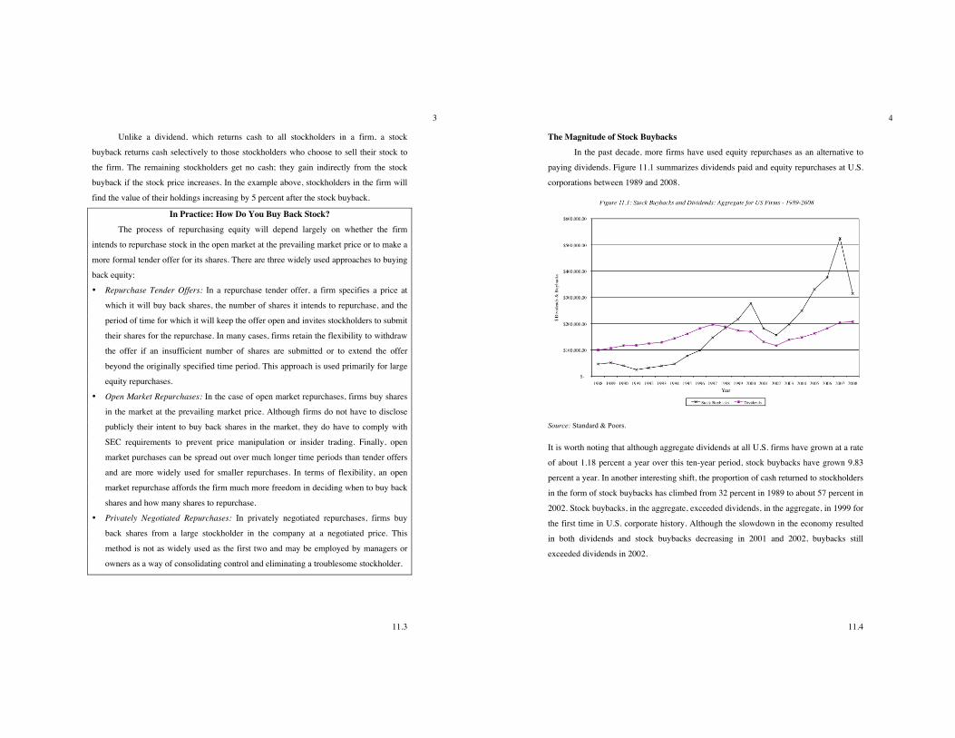
The Magnitude of Stock Buybacks In the past decade, more firms have used equity repurchases as an alternative to

paying dividends. Figure 11.1 summarizes dividends paid and equity repurchases at U.S.

corporations between 1989 and 2008.

Source: Standard & Poors.

It is worth noting that although aggregate dividends at all U.S. firms have grown at a rate

of about 1.18 percent a year over this ten-year period, stock buybacks have grown 9.83

percent a year. In another interesting shift, the proportion of cash returned to stockholders

in the form of stock buybacks has climbed from 32 percent in 1989 to about 57 percent in

2002. Stock buybacks, in the aggregate, exceeded dividends, in the aggregate, in 1999 for

the first time in U.S. corporate history. Although the slowdown in the economy resulted

in both dividends and stock buybacks decreasing in 2001 and 2002, buybacks still

exceeded dividends in 2002.

11.5

5

This shift has been much less dramatic outside the United States. Firms in other

countries have been less likely to use stock buybacks to return cash to stockholders for a

number of reasons.2 First, until 2003, dividends in the United States faced a much higher

tax burden, relative to capital gains, than dividends paid in other countries. Many

European countries, for instance, allow investors to claim a tax credit on dividends to

compensate for taxes paid by the firms paying them. Stock buybacks, therefore, provided

a much greater tax benefit to investors in the United States than they did to investors

outside the United States by shifting income from dividends to capital gains. Second,

stock buybacks were prohibited or tightly constrained in many countries, at least until

very recently. Third, a strong reason for the increase in stock buybacks in the United

States was pressure from stockholders on managers to pay out idle cash. This pressure

was far less in the weaker corporate governance systems that exist outside the United

States.

For the rest of this section, we will be using the phrase “dividend policy” to mean

not just what gets paid out in dividends but also the cash returned to stockholders in the

form of stock buybacks.

Illustration 11.1 Dividends and Stock Buybacks: Disney, Aracruz, Tata Chemicals and

Deutsche Bank

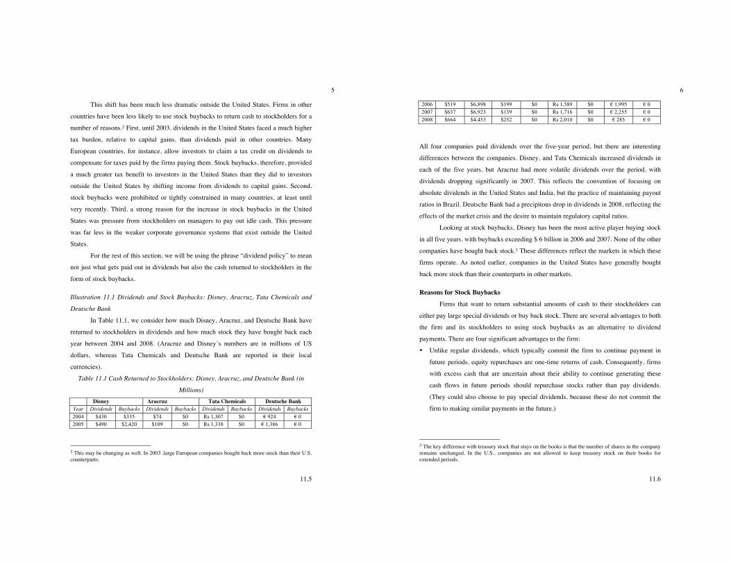
In Table 11.1, we consider how much Disney, Aracruz, and Deutsche Bank have

returned to stockholders in dividends and how much stock they have bought back each

year between 2004 and 2008. (Aracruz and Disney’s numbers are in millions of US

dollars, whereas Tata Chemicals and Deutsche Bank are reported in their local

currencies).

Table 11.1 Cash Returned to Stockholders: Disney, Aracruz, and Deutsche Bank (in

Millions) Disney Aracruz Tata Chemicals Deutsche Bank

Year Dividends Buybacks Dividends Buybacks Dividends Buybacks Dividends Buybacks 2004 $430 $335 $74 $0 Rs 1,307 $0 ! 924 ! 0 2005 $490 $2,420 $109 $0 Rs 1,338 $0 ! 1,386 ! 0

2 This may be changing as well. In 2003 ,large European companies bought back more stock than their U.S. counterparts.

11.6

6

2006 $519 $6,898 $199 $0 Rs 1,589 $0 ! 1,995 ! 0 2007 $637 $6,923 $139 $0 Rs 1,716 $0 ! 2,255 ! 0 2008 $664 $4,453 $252 $0 Rs 2,010 $0 ! 285 ! 0

All four companies paid dividends over the five-year period, but there are interesting

differences between the companies. Disney, and Tata Chemicals increased dividends in

each of the five years, but Aracruz had more volatile dividends over the period, with

dividends dropping significantly in 2007. This reflects the convention of focusing on

absolute dividends in the United States and India, but the practice of maintaining payout

ratios in Brazil. Deutsche Bank had a precipitous drop in dividends in 2008, reflecting the

effects of the market crisis and the desire to maintain regulatory capital ratios.

Looking at stock buybacks, Disney has been the most active player buying stock

in all five years, with buybacks exceeding $ 6 billion in 2006 and 2007. None of the other

companies have bought back stock.3 These differences reflect the markets in which these

firms operate. As noted earlier, companies in the United States have generally bought

back more stock than their counterparts in other markets.

Reasons for Stock Buybacks

Firms that want to return substantial amounts of cash to their stockholders can

either pay large special dividends or buy back stock. There are several advantages to both

the firm and its stockholders to using stock buybacks as an alternative to dividend

payments. There are four significant advantages to the firm:

• Unlike regular dividends, which typically commit the firm to continue payment in

future periods, equity repurchases are one-time returns of cash. Consequently, firms

with excess cash that are uncertain about their ability to continue generating these

cash flows in future periods should repurchase stocks rather than pay dividends.

(They could also choose to pay special dividends, because these do not commit the

firm to making similar payments in the future.)

3 The key difference with treasury stock that stays on the books is that the number of shares in the company remains unchanged. In the U.S., companies are not allowed to keep treasury stock on their books for extended periods.

11.7

7

• The decision to repurchase stock affords a firm much more flexibility to reverse itself

and spread the repurchases over a longer period than does a decision to pay an

equivalent special dividend. In fact, there is substantial evidence that many firms that

announce ambitious stock repurchases do reverse themselves and do not carry the

plans through to completion.

• Equity repurchases may provide a way of increasing insider control in firms, because

they reduce the number of shares outstanding. If the insiders do not tender their

shares back, they will end up holding a larger proportion of the firm and,

consequently, having greater control.

• Finally, equity repurchases may provide firms with a way of supporting their stock

prices when they are declining.4 For instance, in the aftermath of the stock market

crash of 1987, many firms initiated stock buyback plans to keep prices from falling

further with partial success.

There are two potential benefits that stockholders might perceive in stock buybacks:

• Equity repurchases may offer tax advantages to stockholders. This was clearly true

before 2003, because dividends were taxed at ordinary tax rates, whereas the price

appreciation that results from equity repurchases wass taxed at capital gains rates.

Even when dividends and capital gains are taxed at the same rate, stockholders have

the option not to sell their shares back to the firm and therefore do not have to realize

the capital gains in the period of the equity repurchases whereas they have no choice

when it comes to dividends.

• Equity repurchases are much more selective in terms of paying out cash only to those

stockholders who need it. This benefit flows from the voluntary nature of stock

buybacks: Those who need the cash can tender their shares back to the firm, and those

who do not can continue to hold on to them.

In summary, equity repurchases allow firms to return cash to stockholders and still

maintain flexibility for future periods.

4This will be true only if the price decline is not supported by a change in the fundamentals—drop in earnings, declining growth, and so on. If the price drop is justified, a stock buyback program can, at best, provide only temporary respite.

11.8

8

Intuitively, we would expect stock prices to increase when companies announce

that they will be buying back stock. Studies have looked at the effect on stock price of the

announcement that a firm plans to buy back stock. There is strong evidence that stock

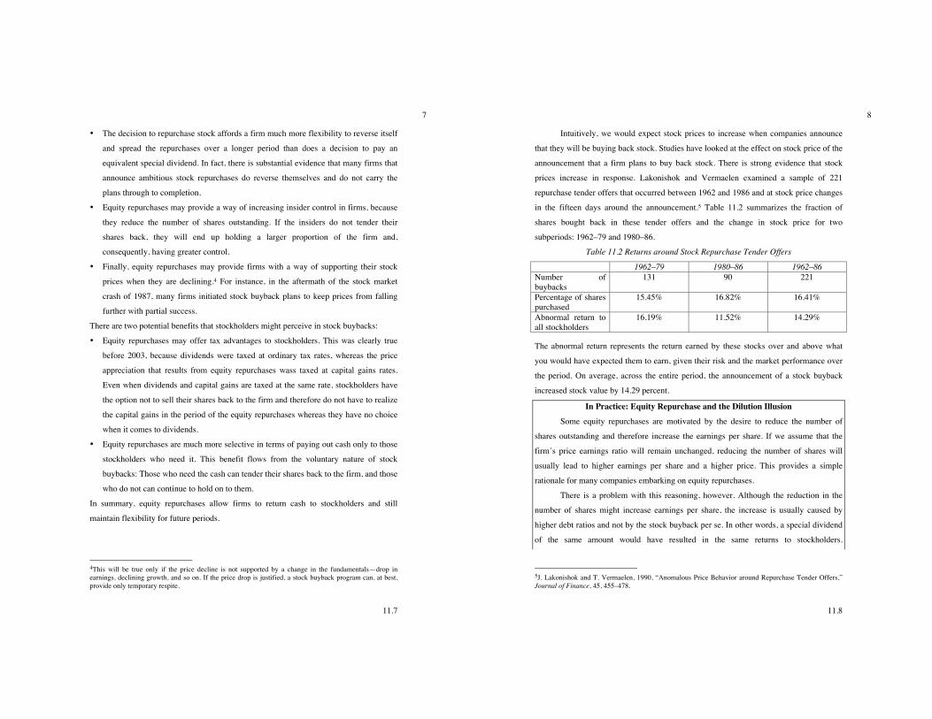
prices increase in response. Lakonishok and Vermaelen examined a sample of 221

repurchase tender offers that occurred between 1962 and 1986 and at stock price changes

in the fifteen days around the announcement.5 Table 11.2 summarizes the fraction of

shares bought back in these tender offers and the change in stock price for two

subperiods: 1962–79 and 1980–86.

Table 11.2 Returns around Stock Repurchase Tender Offers

1962–79 1980–86 1962–86 Number of buybacks

131 90 221

Percentage of shares purchased

15.45% 16.82% 16.41%

Abnormal return to all stockholders

16.19% 11.52% 14.29%

The abnormal return represents the return earned by these stocks over and above what

you would have expected them to earn, given their risk and the market performance over

the period. On average, across the entire period, the announcement of a stock buyback

increased stock value by 14.29 percent.

In Practice: Equity Repurchase and the Dilution Illusion

Some equity repurchases are motivated by the desire to reduce the number of

shares outstanding and therefore increase the earnings per share. If we assume that the

firm’s price earnings ratio will remain unchanged, reducing the number of shares will

usually lead to higher earnings per share and a higher price. This provides a simple

rationale for many companies embarking on equity repurchases.

There is a problem with this reasoning, however. Although the reduction in the

number of shares might increase earnings per share, the increase is usually caused by

higher debt ratios and not by the stock buyback per se. In other words, a special dividend

of the same amount would have resulted in the same returns to stockholders.

5J. Lakonishok and T. Vermaelen, 1990, “Anomalous Price Behavior around Repurchase Tender Offers,” Journal of Finance, 45, 455–478.

11.9

9

Furthermore, the increase in debt ratios should increase the riskiness of the stock and

lower the price earnings ratio. Whether a stock buyback will increase or decrease the

price per share will depend on whether the firm is moving to its optimal debt ratio by

repurchasing stock, in which case the price will increase, or moving away from it, in

which case the price will drop.

To illustrate, assume that an all equity-financed firm in the specialty retailing

business, with 100 shares outstanding, has $100 in earnings after taxes and a market

value of $1,500. Assume that this firm borrows $300 and uses the proceeds to buy back

twenty shares. As long as the after-tax interest expense on the borrowing is less than $20,

this firm will report higher earnings per share after the repurchase. If the firm’s tax rate is

50 percent, for instance, the effect on earnings per share is summarized in the table below

for two scenarios: one where the interest expense is $30 and one where the interest

expense is $55. As long as the interest expense is greater than $ 40 ($20 after taxes), the

firm will report higher earnings per share after the repurchase.

Effect of Stock Repurchase on Earnings per Share

After Repurchase Before Repurchase Interest Expense = $30 Interest Expense = $55

EBIT $200 $200 $200 – Interest $0 $30 $55 = Taxable income

$200 $170 $145

– Taxes $100 $85 $72.50 = Net income $100 $85 $72.50 # Shares 100 80 80 Earnings per share

$1.00 $1.125 $0.91

If we assume that the price earnings ratio remains at 15, the price per share will change in

proportion to the earnings per share. Realistically, however, we should expect to see a

drop in the price earnings ratio as the increase in debt makes the equity in the firm riskier.

Whether the drop will be sufficient to offset or outweigh an increase in earnings per share

will depend on whether the firm has excess debt capacity and whether, by going to a 20

percent debt ratio, it is moving closer to its optimal debt ratio.

11.10

10

Choosing between Dividends and Equity Repurchases Firms that plan to return cash to their stockholders can either pay them dividends

or buy back stock. How do they choose? The choice will depend on the following factors:

• Sustainability and Stability of Excess Cash Flow: Both equity repurchases and

increased dividends are triggered by a firm’s excess cash flows. If the excess cash

flows are temporary or unstable, firms should repurchase stock; if they are stable and

predictable, paying dividends provides a stronger signal of future project quality.

• Stockholder Tax Preferences: If stockholders are taxed at much higher rates on

dividends than capital gains, they will be better off if the firm repurchases stock. If,

on the other hand, stockholders are taxed less on dividends, they will gain if the firm

pays a special dividend.

• Predictability of Future Investment Needs: Firms that are uncertain about the

magnitude of future investment opportunities should use equity repurchases as a way

of returning cash to stockholders. The flexibility that is gained by avoiding what may

be perceived as a fixed obligation will be useful, if they need cash flows in future

periods to fund attractive new investments.

• Undervaluation of the Stock: For two reasons, an equity repurchase makes even more

sense when managers believe their stock is undervalued. First, if the stock remains

undervalued, the remaining stockholders will benefit if managers buy back stock at

less than true value. The difference between the true value and the market price paid

on the buyback will be accrue to those stockholders who do not sell their stock back.

Second, the stock buyback may send a signal to financial markets that the stock is

undervalued, and the market may react accordingly by pushing up the price.

• Management Compensation: Managers often receive options on the stock of the

companies that they manage. The prevalence and magnitude of such option-based

compensation can affect whether firms use dividends or buy back stock. The payment

of dividends reduces stock prices while leaving the number of shares unchanged. The

buying back of stock reduces the number of shares, and the share price usually

increases on the buyback. Because options become less valuable as the stock price

decreases and more valuable as the stock price increases, managers with significant

option positions may be more likely to buy back stock than pay dividends.

11.11

11

Bartov, Krinsky, and Lee examined three of these determinants—undervaluation,

management compensation, and institutional investor holdings (as a proxy for

stockholder tax preferences)—of whether firms buy back stock or pay dividends.6 They

looked at 150 firms announcing stock buyback programs between 1986 and 1992 and

compared these firms to others in their industries that chose to increase dividends instead.

Table 11.3 reports on the characteristics of the two groups.

Table 11.3 Characteristics of Firms Buying Back Stock versus Those Increasing

Dividends

Firms Buying Back

Stock

Firms Increasing

Dividends

Difference Is

Significant

Book/market 56.90% 51.70% Yes

Options/shares 7.20% 6.30% No

# of institutional

holders

219.4 180 yes

Although the option holdings of managers seemed to have had no statistical impact on

whether firms bought back stock or increased dividends, firms buying back stock had

higher book to market ratios than firms increasing dividends and more institutional

stockholders. The higher book to price ratio can be viewed as an indication that these

firms are more likely to view themselves as undervalued. The larger institutional holding

might suggest a greater sensitivity to the tax advantage of stock buybacks.

Stock Buybacks: A Behavioral Perspective

The explosive growth in stock buybacks in the United States in the last two

decades can only partially be explained by financial rationale. In fact, many of the stories

offered for stock buybacks – the tax disadvantages associated with dividends, their

impact on earnings per share – have always been in existence and cannot be used to

rationalize behavior in the last twenty years. There are three behavioral rationale that

have been offered for the growth of buybacks:

6E. Bartov, I. Krinsky, and J. Lee, 1998, “Some Evidence on how Companies Choose between Dividends and Stock Repurchases,” Journal of Applied Corporate Finance, 11, 89–96.

11.12

12

a. Herd behavior: In the chapter on capital structure, we noted the pull that industry

averages and peer group behavior have on debt policy. The same phenomenon applies

in dividend policy, as firms attempt to not only keep their dividends in line with the

rest of the sector but attempt to buy back stock to match other firms that may have

done so. The fact that stock buybacks often tend to be clustered in sectors can be

viewed as evidence of this phenomenon.

b. Framing and Anchoring: Earlier in this chapter, we pointed to the dividend illusion

and noted that the increases in earnings per share that follow stock buybacks will not

always translate into higher price per share, since the price earnings will decrease to

reflect the higher risk in the firm. To the extent that managers think in per share terms

and have in mind a “right PE ratio” for their firms, they may believe that stock

buybacks always lead to higher stock prices. If investors share these same views,

stock prices will increase in the aftermath of buybacks, at least for the short term.

c. Over optimism: More optimistic managers believe that their stocks are under valued

and are therefore more likely to initiate and carry through stock buybacks than their

less optimistic brethren. Consequently, the same market timing imperatives that drive

financing choices (debt versus equity) affect stock buyback decisions.

In summary, it can be argued that once some firms started buying back stock in the 1980s

and were successful with that tactic (in terms of higher stock prices), other firms imitated

them, thus creating a trend that has continued for more than two decades.

11.1. Stock Buybacks and Stock Price Effects

For which of the following types of firms would a stock buyback be most likely to lead to

a drop in the stock price?

a. Companies with a history of poor project choice

b. Companies that borrow money to buy back stock

c. Companies that are perceived to have great investment opportunities

Explain.

11.13

13

A Cash Flow Approach to Analyzing Dividend Policy Given what firms are returning to their stockholders in the form of dividends or

stock buybacks, how do we decide whether they are returning too much or too little? In

the cash flow approach, we follow four steps. We first measure how much cash is

available to be paid out to stockholders after meeting debt service and reinvestment needs

and compare this amount to the amount actually returned to stockholders. We then have

to consider how good existing and new investments in the firm are. Third, based on the

cash payout and project quality, we consider whether firms should be accumulating more

cash or less. Finally, we look at the relationship between dividend policy and debt policy.

Step 1: Measuring Cash Available to Be Returned to Stockholders To estimate how much cash a firm can afford to return to its stockholders, we

begin with the net income—the accounting measure of the stockholders’ earnings during

the period—and convert it to a cash flow by subtracting out a firm’s reinvestment needs,

broken up into two components:

• Investments in long term assets: Any capital expenditures, defined broadly to include

acquisitions, are subtracted from the net income, because they represent cash

outflows. Depreciation and amortization, on the other hand, are added back in

because they are noncash charges. The difference between capital expenditures and

depreciation is referred to as net capital expenditures and is usually a function of the

growth characteristics of the firm. High-growth firms tend to have high net capital

expenditures relative to earnings, whereas low-growth firms may have low (and

sometimes even negative) net capital expenditures.

• Investments in short term assets: Increases in working capital drain a firm’s cash

flows, whereas decreases in working capital increase the cash flows available to

equity investors. Firms that are growing fast, in industries with high working capital

requirements (retailing, for instance), typically have large increases in working

capital. Because we are interested in the cash flow effects, we consider only changes

in noncash working capital in this analysis.

Finally, equity investors also have to consider the effect of changes in the levels of debt

on their cash flows. Repaying the principal on existing debt represents a cash outflow, but

11.14

14

the debt repayment may be fully or partially financed by the issue of new debt, which is a

cash inflow. Again, netting the repayment of old debt against the new debt issues

provides a measure of the cash flow effects of changes in debt.

Allowing for the cash flow effects of net capital expenditures, changes in working

capital, and net changes in debt on equity investors, we can define the cash flows left

over after these changes as the free cash flow to equity (FCFE):

Free Cash Flow to Equity (FCFE) = Net Income

– (Capital Expenditures – Depreciation)

– (Change in Noncash Working Capital)

+ (New Debt Issued – Debt Repayments)

This is the cash flow available to be paid out as dividends.

This calculation can be simplified if we assume that the net capital expenditures

and working capital changes are financed using a fixed mix of debt and equity.7 If ! is the

proportion of the net capital expenditures and working capital changes raised from debt

financing, the effect on cash flows to equity of these items can be represented as follows:

Equity Reinvestment Associated with Capital Expenditure Needs = (Capital

Expenditures – Depreciation) (1 – !)

Equity Reinvestment Associated with Working Capital Needs = (" Non-cash

Working Capital) (1 – !)

Accordingly, the cash flow available for equity investors after meeting capital

expenditure and working capital needs is:

Free Cash Flow to Equity = Net Income

– (Capital Expenditures – Depreciation) (1 – !)

– (" Non-cash Working Capital) (1 – !)

Note that the net debt payment item is eliminated, because debt repayments are

financed with new debt issues to keep the debt ratio fixed. If the target or optimal debt

ratio of the firm is used to forecast the free cash flow to equity that will be available in

future periods, it is particularly useful to assume that a specified proportion of net capital

expenditures and working capital needs will be financed with debt. Alternatively, in

7The mix has to be fixed in book value terms.

11.15

15

examining past periods, we can use the firm’s average debt ratio over the period to arrive

at approximate free cash flows to equity.

In Practice: Estimating the FCFE at a Financial Service Firm Estimating FCFE is straightforward for most manufacturing firms, because the net

capital expenditures, noncash working capital needs, and debt ratio can be obtained from

the financial statements. In contrast, the estimation of FCFE is difficult for financial

service firms for several reasons. First, estimating net capital expenditures and noncash

working capital for a bank or insurance company is difficult because all the assets and

liabilities are in the form of financial claims. Second, it is difficult to define short-term

debt for financial service firms, again due to the complexity of their balance sheets.

To estimate the FCFE for a bank, we redefine reinvestment as investment in

regulatory capital. After all, a financial service firm can grow its business only to the

extent that its has the book value of equity to back up that growth and maintain regulatory

capital ratios (including any safety buffers that it may have built in). In chapter 8, we

looked at regulatory capital ratios and how they affect financing choices at banks and

insurance companies. Since any dividends paid deplete equity capital and retained

earnings increase that capital, the free cash flow to equity for a financial service firm can

be written as follows:

FCFEBank= Net Income – Increase in Regulatory Capital Base (Book Equity)

As a simple example, consider a bank with $ 10 billion in loans outstanding and book

equity (Tier 1 capital) of $ 750 million. Assume that the bank wants to maintain its

existing capital ratio of 7.5%, intends to grow its loan base by 10% (to $11 billion) and

expects to generate $ 150 million in net income next year. We can estimate the FCFE

next year:

FCFE = $150 million – (11,000-10,000)* (.075) = $75 million

As a follow up, assume that this bank wants to increase its regulatory capital ratio to 8%

(for precautionary purposes) while increasing its loan base to $ 11 billion. The total book

equity next year will have to rise to $880 million (8% of $ 11 billion) and the FCFE will

be lower:

FCFE = $ 150 million – ($ 880 - $750) = $20 million

11.16

16

This computation obviously becomes more complex if a firm is involved in multiple

businesses, with different regulatory capital requirements on each. To estimate FCFE, we

have to estimate growth and capital requirements in each business separately.

Putting together the pieces, the FCFE (and potential dividends) at a financial service

firm will be a function of the following:

a. Growth in asset base: Since the regulatory capital is tied to the size of the asset base,

the higher the growth rate in the asset base, the greater will be the investment in

regulatory capital. Holding all else constant, higher growth firms should have lower

FCFE and dividends than more mature firms.

b. Desired capital ratio: The reinvestment in regulatory capital, for a given growth rate in

the asset base, will depend upon the equity capital ratio that the firm wants to maintain on

that asset base. While regulatory requirements play a key role in determining this ratio, it

will also depend upon the safety buffer the firm desires to build into its capital. Put more

simply, conservative financial service firms will have higher target capital ratios and

reinvest more than more aggressive firms, for a given growth rate, leading to lower FCFE

for the former.

c. Profitability: Ultimately, dividends have to be paid out of net income. Other things

remaining equal, the more profits that a firm can generate on a given asset and book

equity base, the more it will be able to generate in FCFE. The return on equity, which

scales profits to book equity capital, therefore becomes a key factor in how much a firm

can generate in FCFE. Firm that generate higher returns on equity, for a given growth

rate and desired capital ratio, will generate more in FCFE.

DividendsBank.xls: This spreadsheet allows you to estimate the free cash flow to

equity for a financial service firm for the future.

Illustration 11.2 Estimating FCFE: Disney, Aracruz, Tata Chemicals and Deutsche Bank

In Table 11.4, we estimate the FCFE for Disney from 1999 to 2008, using

historical information from their financial statements.

Table 11.4 Estimates of FCFE for Disney: 1999-2008 (in millions)

Year Net Income

Capital Expenditures

Depreciation Chg in WC

Change in Net Debt

FCFE

11.17

17

1999 $1,300 $6,113 $3,779 -$363 $176 -$495 2000 $920 $1,091 $2,195 -$1,184 $2,118 $5,326 2001 -$158 $2,015 $1,754 $244 -$77 -$740 2002 $1,236 $3,176 $1,042 $27 -$1,892 -$2,817 2003 $1,267 $1,034 $1,077 -$264 $1,145 $2,719 2004 $2,345 $1,484 $1,210 $51 $2,203 $4,223 2005 $2,533 $1,691 $1,339 $270 $699 $2,610 2006 $3,374 $1,300 $1,437 -$136 -$941 $2,706 2007 $4,687 $627 $1,491 $45 -$2,696 $2,810 2008 $4,427 $2,162 $1,582 $485 -$528 $2,834

Aggregate $21,931 $20,693 $16,906 -$825 $207 $19,176 Average $21 $1,918

The depreciation numbers also include amortization and the capital expenditures include

cash acquisitions. Increases in noncash working capital, shown as positive numbers,

represent a drain on the cash, whereas decreases in noncash working capital, shown as

negative numbers, represent positive cash flows. In 1999, for example, noncash working

capital decreased by $363 million, increasing the cash available for stockholders in that

year by the same amount. Finally, the net cash flow from debt is the cash generated by

the issuance of new debt, netted out against the cash outflow from the repayment of old

debt. Again, using 1999 as an example, Disney issued $176 million more in new debt

than it paid off on old debt, and this represents a positive cash flow in that year. We have

computed two measures of FCFE, one before the net debt cash flow and one after. Using

1999 as an illustration, we compute each as follows:

FCFEBefore Debt CF= Net Income + Depreciation – Capital Expenditures – Change in

Noncash Working Capital = 1300+3779-6113-(-363) = -$ 671 million

FCFEAfter Debt CF= FCFEBefore Debt CF + Net Debt CF = -$671 + $176 = -$495 million

As Table 11.4 indicates, Disney had negative free cash flows to equity in three of the ten

years. The average annual FCFE before net debt issues over the period was $1918

million, and the average net debt issued over the period was $21 million, resulting in an

average annual FCFE after net debt issues of $1,939 million. We can compute Disney’s

FCFE each year using the approximation that we described in the last section. To do this,

we first have to compute the net debt cash flows as percent of reinvestment needs over

this period. Using the aggregate values from table 11.4 for debt cash flows, capital

11.18

18

expenditures, depreciation, and changes in noncash working capital between 1999 and

2008, we estimate the average debt ratio:

Average Debt Ratio =

!

Net Debt Issued(Cap Ex - Depreciation + Chg in WC)

!

=207

(20,693 - 16,906 - 825) =6.99%

The FCFE each year can then be estimated using the average debt ratio, instead of the

actual net debt cash flows. Table 11.5 contains the estimates of FCFE each year using

this approach for Disney.

Table 11.5. Approximate FCFE for Disney from 1999 to 2008 (in millions)

Year Net Income

(Cap Ex - Depreciation) (1-DR)

Chg in WC (1-DR)

FCFE

1999 $1,300 $2,171 -$338 -$533 2000 $920 -$1,027 -$1,101 $3,048 2001 -$158 $243 $227 -$628 2002 $1,236 $1,985 $25 -$774 2003 $1,267 -$40 -$246 $1,553 2004 $2,345 $255 $47 $2,043 2005 $2,533 $327 $251 $1,954 2006 $3,374 -$127 -$126 $3,628 2007 $4,687 -$804 $42 $5,449 2008 $4,427 $539 $451 $3,436 Aggregate $21,931 $3,522 -$767 $19,176 Average $1,918

Note that the average FCFE between 1999 and 2008 remains unchanged at $1,918

million a year when we use the approximation. The FCFE in each year is different,

though, from the estimates in Table 11.5, because we are smoothing out the effects of the

cash flows from debt.

A similar estimation of FCFE was done for Aracruz from 2002 to 2008 in Table

11.6, again using historical information. Since the cash flow statement in US dollars,

filed in the United States, is more complete than the $R counterpart, we will report all the

values in US dollars.

Table 11.6 FCFE for Aracruz in US$ from 2002 to 2008 (in millions) Year Net Capital Depreciation Change in Change in Net FCFE

11.19

19

Income Expenditures WC Debt 2002 $111.91 $260.66 $171.53 $53.53 $36.34 $5.59 2003 $148.09 $791.87 $191.51 $79.85 $530.69 -$1.43 2004 $227.24 $193.54 $206.95 $31.80 -$13.53 $195.32 2005 $341.10 $216.98 $211.62 $75.55 -$93.40 $166.79 2006 $455.32 $325.51 $217.84 $72.20 -$89.60 $185.85 2007 $422.07 $712.48 $217.64 $113.71 $112.28 -$74.20 2008 -$1,239.00 $814.60 $218.05 $61.50 $3,025.00 $1,127.95

Aggregate $466.73 $3,315.64 $1,435.14 $488.14 $3,507.78 $1,605.87 Average FCFE: 2002-2008 $229.41 Average FCFE: 2002-2007 $79.65

Average FCFE without debt cash flows -$271.70

Between 2002 and 2007, Aracruz reported an almost four-fold increase in net income, but

aggregate free cash flows to equity averaged only $79.65 million a year, over the period.

In 2008, Aracruz reported a net loss of $1.239 billion, largely because of misguided betas

on currency derivatives, but the FCFE for 2008 was positive, as the firm borrowed more

than $ 3 billion to cover its losses. The average FCFE over the 2002-08 time period is

$229.41 million, with the cash flows from debt counted in, but -$271.70 million, without

debt cash flows.

Using the same procedure, we estimate the FCFE for Tata Chemicals from 2004

to 2008 in table 11.7:

Table 11.7 FCFE for Tata Chemicals from 2003 to 2008 (in millions) Year Net

Income Capital Expenditures

Depreciation Change in WC

Change in Net Debt

FCFE

2003-04 Rs 3,418 Rs 357 Rs 1,442 -Rs 557 -Rs 2,771 Rs 2,289 2004-05 Rs 4,550 Rs 692 Rs 1,377 -Rs 493 Rs 5,448 Rs11,176 2005-06 Rs 5,156 Rs 11,730 Rs 1,389 Rs 2,823 Rs 867 -Rs7,141 2006-07 Rs 6,338 Rs 1,196 Rs 1,504 -Rs 1,662 -Rs 4,411 Rs 3,896 2007-08 Rs 11,571 Rs 28,956 Rs 1,488 Rs 88 Rs 17,054 Rs 1,069 Aggregate Rs 31,033 Rs 42,930 Rs 7,199 Rs 200 Rs 16,187 Rs11,290 Average Rs 2,258

While the net income for Tata Chemicals increased every year between 2003 and 2008,

the FCFE follow a rockier path, with big swings in the cash flows for three reasons. The

first is that non-cash working capital is volatile, with big increases in some years and

large decreases in others. The second is that there are spikes in the capital expenditures in

2005-06 and 2007-08, reflecting large investments in subsidiaries in those years. Finally,

the cash flow from net debt is negative in two of the five years and is a very large

11.20

20

positive number in 2007-08, reflecting the fact that Tata funded its large capital

expenditures that year, primarily with debt. Over the five-year period, the average FCFE

was Rs 2.258 billion.

To estimate the FCFE for Deutsche Bank, we use the approach described in the

last section, where we define reinvestment in regulatory capital as reinvestment. Rather

than look backwards, we decided to focus on estimating future FCFE,. We begin with the

current values for the asset base and regulatory capital at the end of 2008:

Current value of Asset Base (end of 2008) = 312.885 billion Euros

Current value of Regulatory Capital (Book Equity) = 31.914 billion Euros

While Deutsche Bank reported a loss of 4.12 billion Euros in 2008, much of the loss can

be attributed to write-offs of investments, in the aftermath of the market crisis in the last

quarter of 2008. Though it is unlikely that Deutsche Bank will revert back to the 6 billion

Euros in profits it reported in 2007, we assume that the normalized net income for 2008

will be 3 billion Euros.8 With these estimates, we obtain a current regulatory capital ratio

of 10.2% and a current return on equity of 9.40%:

Current Regulatory Capital Ratio =

!

Regulatory CapitalAsset Base

=31,914312,885

=10.2%

Current Return on Equity =

!

Net IncomeRegulatory Capital (Book Equity)

=3.00

31,914= 9.40%

As a final piece for the estimation of FCFE, we estimate three values. First, we assume

that the expected growth in the asset base will be 4% a year for the next 5 years and 3%

thereafter. Second, we assume a target regulatory capital ratio of 10% in year 5, based on

Deutsche Bank’s own statements in early 2009; note that this value is well above the

regulatory requirement of 6-7% and reflects Deutsche Bank’s conservative outlook.

Third, we assume only a modest improvement in the return on equity from the current

value of 9.40% to 10% in year 5 and beyond.

To estimate the regulatory capital and net income in each of the next 5 years, we

assume that the improvements will occur in equal annual increments over each of the

8 To normalize the net income, we looked at profits prior to write offs. In the first quarter of 2009, Deutsche Bank reported a bounce back to profitability, generating 1.2 billion in Euros in profits. Analysts estimate that Deutsche will generate profits in excess of 4 billion Euros for the year, but we have chosen to be conservative in our estimates.

11.21

21

years. Table 11.8 summarizes the estimates of regulatory capital, net income and FCFE

for the next six years.

Table 11.8: Expected FCFE – Deutsche Bank (in millions of Euros)

Current 2009 2010 2011 2012 2013 Steady state

(2014)

Asset Base 312,882 !

325,398 !

338,414 !

351,950 !

366,028 !

380,669 ! 392,089 !

Capital ratio 10.20% 10.16% 10.12% 10.08% 10.04% 10.00% 10.00%

Regulatory Capital 31,914 !

33,060 !

34,247 !

35,477 !

36,749 !

38,067 ! 39,209 !

Change in regulatory capital 1,146 ! 1,187 ! 1,229 ! 1,273 ! 1,318 ! 1,142 ! ROE 9.40% 9.52% 9.64% 9.76% 9.88% 10.00% 10.00% Net Income 3,000 ! 3,147 ! 3,302 ! 3,463 ! 3,631 ! 3,807 ! 3,921 ! - Investment in Regulatory Capital 1,146 ! 1,187 ! 1,229 ! 1,273 ! 1,318 ! 1,142 ! FCFE 2,001 ! 2,114 ! 2,233 ! 2,358 ! 2,489 ! 2,779 !

Based on our estimates, Deutsche Bank should be able to return about 2 billion in Euros

in dividends in 2009 to its equity investors. Note, though, that the regulatory definition of

equity includes both preferred and common stockholders and that preferred stockholders

have fixed and prior claims to the dividends; the dividends to common stockholders

represent the residual FCFE. Just as an illustration assume that Deutsche Bank’s existing

capital base includes 5 billion Euros in preferred stock with a dividend set at 8% of face

value. The FCFE available for common stockholders in 2009 can then be computed as

follows:

Total FCFE in 2009 = 2,001 million Euros

Preferred Dividends = .08 (5,000) = 400 million Euros

FCFE for common equity = 1,601 million Euros

This can be repeated for subsequent years.

11.2. Defining FCFE

The reason that the net income is not the amount that a company can afford to pay out in

dividends is because

a. earnings are not cash flows.

b. some of the earnings have to be reinvested back in the firm to create growth.

c. there may be cash inflows or outflows associated with the use of debt.

11.22

22

d. all of the above.

Explain.

Measuring the Payout Ratio

The conventional measure of dividend policy—the dividend payout ratio—gives

us the value of dividends as a proportion of earnings. In contrast, our approach measures

the total cash returned to stockholders as a proportion of FCFE:

Dividend Payout Ratio = Dividends/Earnings

Cash to Stockholders to FCFE Ratio = (Dividends + Equity Repurchases)/FCFE

The ratio of cash returned to stockholders to FCFE shows how much of the cash available

to be paid out to stockholders is actually returned to them in the form of dividends and

stock buybacks. If this ratio over time is equal or close to 100 percent, the firm is paying

out all that it can to its stockholders. If it is significantly less than 100 percent, the firm is

paying out less than it can afford and is using the difference to increase its cash balance

or to invest in marketable securities. If it is significantly over 100 percent, the firm is

paying out more than it can afford and is either drawing on an existing cash balance or

issuing new securities (stocks or bonds).

Illustration 11.3 Comparing Dividend Payout Ratios to FCFE Payout Ratios: Disney and

Tata Chemicals

In the following analysis, we compare the dividend payout ratios to the cash to

stockholders (dividends and stock buybacks) as a percent of FCFE for Disney and Tata

Chemicals. Table 11.9 shows both numbers for Disney from 1999 to 2008.

Table 11.9 Disney: Dividends as Percentage of Earnings and Cash Returned as

Percentage of FCFE

Year Dividends Earnings Payout Ratio Cash Returned FCFE Cash/FCFE 1999 $0.00 $1,300.00 0.00% $19.00 -$495.00 -3.84% 2000 $434.00 $920.00 47.17% $600.00 $5,326.00 11.27% 2001 $438.00 -$158.00 -277.22% $1,511.00 -$740.00 -204.19% 2002 $428.00 $1,236.00 34.63% $428.00 -$2,817.00 -15.19% 2003 $429.00 $1,267.00 33.86% $429.00 $2,719.00 15.78% 2004 $430.00 $2,345.00 18.34% $765.00 $4,223.00 18.12% 2005 $490.00 $2,533.00 19.34% $2,910.00 $2,610.00 111.49% 2006 $519.00 $3,374.00 15.38% $7,417.00 $2,706.00 274.09% 2007 $637.00 $4,687.00 13.59% $7,560.00 $2,810.00 269.04%

11.23

23

2008 $664.00 $4,427.00 15.00% $5,117.00 $2,834.00 180.56% Aggregate $4,469.00 $21,931.00 20.38% $26,756.00 $19,176.00 139.53%

As you can see, Disney paid out 20.38 percent of its aggregate earnings as dividends over

this period.9 Over the same period, it returned 139.53 percent of its FCFE to its

stockholders in the form of dividends and stock buybacks. Though the payout ratio

suggests that the firm is retaining a significant portion of its earnings, the cash returned as

a percent of FCFE suggests that Disney has paid out far more than it had available to pay

during the period.

Table 11.10 shows dividend payout ratios and cash returned to stockholders as a

percent of FCFE for Tata Chemicals from 2002 to 2008.

Table 11.10 Tata Chemicals: Dividends as Percentage of Earnings and Cash Returned as

Percent of FCFE (in millions)

Year Dividends Net Income Payout ratio Cash returned FCFE Cash/FCFE 2003-04 Rs 1,306.50 Rs 3,418.40 38.22% Rs1,306.50 Rs 2,289.10 57.07% 2004-05 Rs 1,338.20 Rs 4,550.00 29.41% Rs1,338.20 Rs 11,176.40 11.97% 2005-06 Rs 1,589.30 Rs 5,155.60 30.83% Rs 1,589.30 -Rs 7,140.90 -22.26% 2006-07 Rs 1,715.70 Rs 6,338.40 27.07% Rs 1,715.70 Rs 3,896.30 44.03% 2007-08 Rs 2,009.60 Rs 11,571.00 17.37% Rs 2,009.60 Rs 1,068.60 188.06% Aggregate Rs 7,959.30 Rs 31,033.40 25.65% Rs 7,959.30 Rs 11,289.50 70.50%

Tata paid out about 25.7% of its earnings as dividends and returned about 70.5% of its

FCFE to its stockholders. The remaining potential dividend (the 29.5% of FCFE that did

not get paid out) was held back by the firm and reinvested in other firms in the Tata

group.

With Aracruz, the comparison is moot, since we know that the aggregate FCFE

would have been negative between 2002 and 2008 without the significant borrowings in

2008 (see table 11.6). Since Aracruz paid out significant dividends over this period, it is

quite clear that these dividends are not being funded from operations. We will return to

examine both why Aracruz is in this bind and ways that it may be able to release itself

from the cash flow constraint in future years.

9To compute the payout ratio over the entire period, we first aggregated earnings and dividends over the entire period and then divided the aggregate dividends by the aggregate earnings. This avoids the problems created by averaging ratios where outliers (very high ratios) are common.

11.24

24

Dividends.xls: This spreadsheet allows you to estimate the free cash flow to equity

and the cash returned to stockholders for a period of up to ten years.

There is a data set online that summarizes dividends, cash returned to stockholders,

and FCFE by sector in the United States.

Why Firms May Not Pay Out What Is Available

For several reasons, many firms pay out less to stockholders, in the form of

dividends and stock buybacks, than they have available in free cash flows to equity. The

reasons vary from firm to firm and we list some here.

• The managers of a firm may gain by retaining cash rather than paying it out as a

dividend. The desire for empire building makes increasing the size of the firm an

objective on its own. Alternatively, management may feel the need to build up a cash

cushion to tide them over periods when earnings may dip; in such periods, the cash

cushion may help buffer the earnings drop and may allow managers to remain in

control.

• The firm may be unsure about its future financing needs and may choose to retain

some cash to take on unexpected investments or meet unanticipated needs.

• The firm may have volatile earnings and may retain cash to help smooth out

dividends over time.

• Bondholders may impose restrictions on cash payments to stockholders, which may

prevent the firm from returning available cash flows to its stockholders.

At the other end of the spectrum, there are firms that pay out more cash than they

generate in FCFE though this is a less common phenomenon. Here again, there are

several possible reasons.

• When earnings are volatile and swing from period to period, firms may choose to pay

more than their FCFE in down periods and hope to make up for it when earnings

recover.

• Firms that have historically paid high dividends often are under pressure to maintain

those dividends even when earnings drop, for fear of sending a bad signal to the

market.

11.25

25

• Firms that are under levered can use a policy of returning more cash to their

stockholders as a way of reducing equity and increasing debt ratios

Finally, firms that are part of larger groups, as Tata Chemicals illustrates, can hold back

cash to invest in other companies in the group.

11.3. What Happens to the FCFE that Are Not Paid Out? In 2003, Microsoft had FCFE of roughly $9 billion, paid no dividends, and bought back

no stock. Where would you expect to see the difference of $9 billion show up in

Microsoft’s financial statements?

a. It will be invested in new projects.

b. It will be in retained earnings, increasing the book value of equity.

c. It will increase the cash balance of the company.

d. None of the above.

Explain.

Evidence on Dividends and FCFE

We can observe the tendency of firms to pay out less to stockholders than they

have available in FCFE by examining cash returned to stockholders paid as a percentage

of FCFE. In 2008, for instance, the median cash returned to FCFE ratio across dividend

paying firms listed in the United States was about 55%. However, there were scores of

firms that paid out more in dividends than they have available in FCFE. Figure 11.2

provides a breakdown of US firms in 2008, based upon how much they paid in dividends,

relative to what they had available in FCFE.

11.26

26

Source: Value Line, 2008.

Note that there are about 755 firms that pay less in dividends than they have available in

FCFE, and they have to finance these dividend payments either out of existing cash

balances or by making new stock and debt issues. Note that there are 550 firms in this

period that paid dividends even though they had negative FCFE. These firms will have to

come up with enough funds, either from existing cash balances or new stock issues, to

cover both the dividends and the cash deficit. A large number of firms (3011) pay no

dividends but that makes sense, given the fact that they have negative FCFE.

That still leaves us with 2555 firms that pay out no dividends, even though they

have positive FCFE, and about 805 firms that pay out less in dividends than they have

available in FCFE. However, that does not necessarily mean that these firms are

accumulating cash, since some of them buy back their own stock in large quantities. With

the rest of the firms, the cash that is not paid out is accumulated as a balance and it does

help explain how some firms end up with outsized cash balances, relative to value.

Dividends.xls: This spreadsheet allows you to estimate the FCFE for a firm over a

period for up to ten years and compare it to dividends paid.

11.27

27

Step 2: Assessing Project Quality The alternative to returning cash to stockholders is reinvestment. Consequently, a

firm’s investment opportunities influence its dividend policy. Other things remaining

equal, a firm with better projects typically has more flexibility in setting dividend policy

and defending it against stockholder pressure for higher dividends. But how do we define

a good project?

According to our analysis of investment decisions, a good project is one that earns

at least the hurdle rate, which is the cost of equity if cash flows are estimated on an equity

basis, or the cost of capital if cash flows are measured on a pre-debt basis. In theory, we

could estimate the expected cash flows on every project available to the firm and

calculate the internal rates of return (IRR) or net present value (NPV) of each project to

evaluate project quality. There are several practical problems with this, however. First,

we have to be able to obtain the detailed cash flow estimates and hurdle rates for all

available projects, which can be daunting if the firm has dozens or even hundreds of

projects. The second problem is that even if these cash flows are available for existing

projects, they will not be available for future projects.

As an alternative approach to measuring project quality, we can use one or more

of the measures we developed in Chapter 5 to evaluate a firm’s current project portfolio:

• Accounting return differentials, where we compare the accounting return on equity to

the cost of equity and the accounting return on capital to the cost of capital.

• Economic value added (EVA), which measures the excess return earned on capital

invested in existing investments and can be computed either on an equity or capital

basis.

We did note the limitations of each of these approaches in Chapter 5, but they still

provide a measure of the quality of a firm’s existing investments.

Using past project returns as a measure of future project quality can result in

errors if a firm is making a transition from one stage in its growth cycle to the next or if it

is in the process of restructuring. In such situations, it is entirely possible that the

expected returns on new projects will differ from past project returns. Consequently, it

may be worthwhile scrutinizing past returns for trends that may carry over into the future.

The average return on equity or capital for a firm will not reveal these trends very well

11.28

28

because they are slow to reflect the effects of new projects, especially for large firms. An

alternative accounting return measure, which better captures year-to-year shifts, is the

marginal return on equity or capital, which is defined as follows:

Marginal Return on Equityt =

!

Net Incomet "Net Incomet -1Book Value of Equityt -1 - Book Value of Equityt -2

Marginal Return on Capital =

!

EBIT(1" t)t " EBIT(1" t)t -1Book Value of Capitalt -1 - Book Value of Capitalt -2

Although the marginal return on equity (capital) and the average return on equity

(capital) will move in the same direction, the marginal returns typically change much

more than do the average returns, the difference being a function of the size of the firm.

These marginal returns can be used to compute the quality of the new projects.

The alternative to using accounting returns to measure the quality of a firm’s

projects is to look at how well or badly a firm’s stock has done in financial markets. In

Chapter 4, we compared the returns earned by a stock to the returns earned on the market

after adjusting for risk (Jensen’s Alpha). The risk-adjusted excess return that we

estimated becomes a measure of whether a stock has under- or outperformed the market.

A positive excess return would then be viewed as an indication that a firm has done better

than expected, whereas a negative excess return would indicate that a firm has done

worse than anticipated.

Finally, accounting income and stock returns may vary year to year, not only

because of changes in project quality but also because of fluctuations in the business

cycles and interest rates. Consequently, the comparisons between returns and hurdle rates

should be made over long enough periods, say, five to ten years, to average out these

other effects.

Illustration 11.4 Evaluating Project Quality at Disney, Aracruz and Tata Chemicals

In Illustration 6.10, we examined the quality of existing investments at Disney,

Aracruz and Tata Chemicals, using both accounting returns and EVA and stock price

performance at each of these companies was evaluated using Jensen’s alpha in chapter 4.

Table 11.11 summarizes our findings.

Table 11.11: Project Returns and Stock Price Performance

11.29

29

ROC Cost of capital

ROC - Cost of capital

ROE Cost of equity

ROE - Cost of Equity

Jensen's Alpha

Disney 9.29% 7.51% 1.78% 14.40% 8.91% 5.49% 5.62% Aracruz 4.49% 10.63% -6.14% -78.59% 18.45% -97.05% 9.97% Tata Chemicals

11.31% 11.44% -0.12% 15.46% 13.93% 1.53% -4.29%

In summary, we concluded that Disney earns positive excess returns on its projects, Tata

Chemicals breaks even and that Aracruz earns negative excess returns and that the stock

price performance reflects these excess returns.

In the following analysis, we revisit both accounting and market measures of

return at Disney, Aracruz and Tata Chemicals over recent time periods and compare them

to the appropriate hurdle rates to evaluate the quality of the projects taken at each firm

during the period. In this analysis, though, we could be faulted for focusing on

performance over short time periods and failing to adjust the cost of equity for actual

market performance. We will try to remedy both defects in this illustration.

We begin with an analysis of Disney’s accounting return on equity, the return

from holding the stock, and the required return (given the beta and market performance

during each year) from 1999 to 2008 as shown in Table 11.12.10

Table 11.12 Return on Equity, Return on Stock, and Cost of Equity: Disney

Year ROE Return on

Stock Cost of Equity

Accounting Excess Return

Market Excess Return

1999 6.71% -1.80% 19.27% -12.56% -21.07% 2000 4.39% -0.36% -7.57% 11.96% 7.21% 2001 -0.66% -27.68% -10.31% 9.66% -17.37% 2002 5.45% -20.27% -19.64% 25.09% -0.63% 2003 5.40% 44.36% 25.70% -20.30% 18.65% 2004 9.86% 20.19% 9.77% 0.09% 10.42% 2005 9.71% -12.81% 4.67% 5.05% -17.48% 2006 12.87% 44.25% 14.54% 12.87% 29.71% 2007 14.73% -3.49% 5.40% 9.33% -8.89% 2008 14.40% -28.62% -32.81% 47.20% 4.18%

* Cost of Equity = Riskfree rate at start of year + Beta (Return on S&P 500 for year – Riskfree rate)

10 For instance, to estimate the expected return in 1999, we use the following: Expected Return in 1999 = Risk-Free Rate at Beginning of 1999 + Beta (Return on Market in 1999 – Risk-Free Rate at Beginning of 1999). An average beta of 0.9011 was used over the entire period for Disney.

11.30

30

As you can see, the trend lines favor Disney, with negative accounting and market returns

in the early years followed by positive excess returns on both dimensions in recent years.

To provide some history on these measures, the return on equity for the firm, which

exceeded 20% in the years prior to the acquisition of Capital Cities/ABC in 1996,

plummeted in the years after to single digits, and the excess returns were negative for

much of 1997-2004. Since Bob Iger replaced Michael Eisner as CEO in 2005, the

company has done better and its performance may have earned it a reprieve when it

comes to dividend policy.

Repeating this analysis for Aracruz for 2002 to 2008 yields a different conclusion.

Table 11.13 summarizes returns on equity, returns on the stock, and the required return at

the firm for each year between 2002 and 2008.

Table 11.13 Return on Equity, Return on Stock, and Cost of Equity: Aracruz

Year ROE Return on

Stock Cost of Equity Accounting

Excess Return Market Excess

Return 2002 13.90% 6.11% -39.49% 53.39% 45.59% 2003 17.40% 94.57% 48.70% -31.30% 45.87% 2004 25.49% 13.56% 17.73% 7.76% -4.17% 2005 37.70% 11.40% 6.21% 31.49% 5.19% 2006 43.15% 58.50% 23.74% 19.41% 34.76% 2007 32.64% 25.49% 6.10% 26.53% 19.39% 2008 -51.91% -81.91% -64.86% 12.95% -17.05%

For much of this period, Aracruz performed well, earning high returns on equity on its

projects and earning excess returns for its stockholders. However, 2008 was a devastating

year, as losses on derivatives wiped out profits from prior years and the stock price

plummeted. While much of the volatility in earnings and returns from year to year, in

prior years, can be attributed to commodity price variation, the losses in 2008 can be

attributed mostly to failures on the part of management.

Finally, we look at Tata Chemicals and estimate the accounting and market-based

excess returns from 2003-2008 in Table 11.14.

Table 11.14: ROE, Stock Returns and Cost of Equity: Tata Chemicals

Year ROE Return on

Stock Cost of Equity

Accounting Excess Returns

Market Excess Return

2003-04 16.80% 11.53% 14.30% 2.50% -2.77% 2004-05 22.78% 46.14% 42.02% -19.25% 4.12%

11.31

31

2005-06 13.07% -5.28% 45.91% -32.84% -51.19% 2006-07 17.01% 95.29% 45.79% -28.78% 49.50% 2007-08 18.68% -57.81% -48.60% 67.28% -9.21% Average 17.34% 17.97% 19.89% -2.22% -1.91%

Across the five-year period, Tata Chemicals delivered a stock return and return on equity

that roughly matched up to the cost of equity over the period. In effect, the firm’s

performance has been neutral over the period.

Dividends.xls: This spreadsheet allows you to estimate the average return on equity

and cost of equity for a firm for a period of up to ten years.

11.4. Historical, Average, and Projected Returns on Capital You have been asked to judge the quality of the projects available at Super Meats, a meat

processing company. It has earned an average return on capital of 10 percent over the

previous five years, but its marginal return on capital last year was 14 percent. The

industry average return on capital is 12 percent, and it is expected that Super Meats will

earn this return on its projects over the next five years. If the cost of capital is 12.5

percent, which of the following conclusions would you draw about Super Meat’s

projects?

a. It invested in good projects over the last five years.

b. It invested in good projects last year.

c. It can expect to invest in good projects over the next five years.

In terms of setting dividend policy, which of these conclusions matter the most?

In Practice: Dealing with Accounting Returns Accounting rates of return, such as return on equity and capital, are subject to abuse

and manipulation. For instance, decisions on how to account for acquisitions (purchase or

pooling), choice of depreciation methods (accelerated versus straight line), and whether

to expense or capitalize an item (R&D) can all affect reported income and book value. In

addition, in any specific year, the return on equity and capital can be biased upward or

downward depending on whether the firm had an unusually good or bad year. To

estimate a fairer measure of returns on existing projects, we recommend the following:

11.32

32

1. Normalize the income before computing returns on equity or capital. For Aracruz,

using the average income over the past three years, instead of the depressed income in

1996, provides returns on equity or capital that are much closer to the required

returns.

2. Back out cosmetic earnings effects caused by accounting decisions, such as the one

on pooling versus purchase. This is precisely why we should consider Disney’s

income prior to the amortization of the Capital Cities acquisition in computing returns

on equity and capital.

3. If there are operating expenses designed to create future growth, rather than current

income, capitalize those expenses and treat them as part of book value while

computing operating income prior to those expenses. This is what we did with

Bookscape when we capitalized operating leases and treated them as part of the

capital base and used the adjusted values in computing return on capital.

Step 3: Evaluating Dividend Policy Once we have measured a firm’s capacity to pay dividends and assessed its

project quality, we can decide whether the firm should continue its existing policy of

returning cash to stockholders, return more cash, or return less. The assessment will

depend on how much of the FCFE is returned to stockholders each period and how good

the firm’s project opportunities are. There are four possible scenarios:

• A firm may have good projects and may be paying out more (in dividends and stock

buybacks) than its FCFE. In this case, the firm is losing value in two ways. First, by

paying too much in dividends, it creates a cash shortfall that has to be met by issuing

more securities. Second, the cash shortfall often creates capital rationing constraints;

as a result, the firm may reject good projects it otherwise would have taken.

• A firm may have good projects and may be paying out less than its FCFE as a

dividend. Although it will accumulate cash as a consequence, the firm can

legitimately argue that it will have good projects in the future in which it can invest

the cash, though investors may wonder why it did not take the projects in the current

period.

11.33

33

• A firm may have poor projects and may be paying out less than its FCFE as a

dividend. This firm will also accumulate cash, but it will find itself under pressure

from stockholders to distribute the cash because of their concern that the cash will be

used to finance poor projects.

• A firm may have poor projects and may be paying out more than its FCFE as a

dividend. This firm first has to deal with its poor project choices, possibly by cutting

back on those investments that make returns below the hurdle rate. Because the

reduced capital expenditure will increase the FCFE, this may take care of the

dividend problem. If it does not, the firm will have to cut dividends as well.

Figure 11.3 illustrates the possible combinations of cash payout and project quality.

Figure 11.3 Analyzing Dividend Policy Quality of projects taken: ROE versus Cost of Equity

Poor projects Good projects

Cash Surplus + Good ProjectsMaximum flexibility in setting dividend policy

Cash Surplus + Poor ProjectsSignificant pressure to pay out more to stockholders as dividends or stock buybacks

Cash Deficit + Good ProjectsReduce cash payout, if any, to stockholders

Cash Deficit + Poor ProjectsCut out dividends but real problem is in investment policy.

Disney

Aracruz

Tata Chemicals

AppleIntel

In this matrix, Disney with its combination of good investments (at least in recent years)

and too much cash returned to its stockholders falls into the quadrant where reducing the

payout makes sense. Since much of the cash payout is in the form of stock buybacks, this

11.34

34

would suggest that Disney reduce its buybacks. Tata Chemicals, with its combination of

neutral investments and cash build-up, could be targeted for more dividends if the quality

of its projects deteriorates. Finally, Aracruz poses the toughest challenge, since it clearly

is paying out too much in dividends, relative to cash available, but also has the worst

track record of the three companies in terms of project returns and stock price

performance. Reducing dividends is part of the solution but it has to be combined with

more discipline in investment analysis and better risk controls.

Note, however, that the pressure to pay dividends comes from the lack of trust in

management rather than greed on the part of stockholders. For a contrast, consider Apple

and Google, two companies that generated billions in FCFE in 2008 and returned little to

their stockholders, while accumulating large cash balances. The high returns earned on

projects and superior stock price performance at both companies earned them the

flexibility to pay out far less in cash than they generated, with little protest from

stockholders. In contrast, Intel has struggled to convince stockholders to allow it to retain

a large cash balance, largely because its project and stock returns have lagged in recent

years.

Consequences of Payout Not Matching FCFE

The consequences of the cash payout to stockholders not matching the FCFE can

vary depending on the quality of a firm’s projects. In this section, we examine the

consequences of paying out too little or too much for firms with good projects and for

firms with bad projects. We also look at how managers in these firms may justify their

payout policy and how stockholders are likely to react to the justification.

A. Poor Projects and Low Payout

There are firms that invest in poor projects and accumulate cash by not returning

any to stockholders. We discuss stockholder reaction and management response to the

dividend policy.

Consequences of Low Payout

When a firm pays out less than it can afford to in dividends, it accumulates cash.

If a firm does not have good projects in which to invest this cash, it faces several

possibilities. In the most benign case, the cash accumulates in the firm and is invested in

11.35

35

financial assets. Assuming that these financial assets are fairly priced, the investments are

zero NPV projects and should not negatively affect firm value. There is the possibility,

however, that the firm may find itself the target of an acquisition, financed in part by its

large holdings of liquid assets.

In the more damaging scenario, as the cash in the firm accumulates, the managers

may be tempted to invest in projects that do not meet their hurdle rates, either to reduce

the likelihood of a takeover or to earn higher returns than they would on financial

assets.11 These actions will lower the value of the firm. Another possibility is that the

management may decide to use the cash to finance an acquisition. This hurts stockholders

in the firm because some of their wealth is transferred to the stockholders of the acquired

firms. The managers will claim that such acquisitions have strategic and synergistic

benefits. The evidence indicates, however, that most firms that have financed takeovers

with large cash balances, acquired over years of paying low dividends while generating a

high FCFE, have reduced stockholder value.

Stockholder Reaction

Because of the negative consequences of building large cash balances,

stockholders of firms that pay insufficient dividends and do not have “good” projects

pressure managers to return more of the cash. This is the basis for the free cash flow

hypothesis, where dividends serve to reduce free cash flows available to managers and,

by doing so, reduce the losses management actions can create for stockholders.

Management’s Defense

Not surprisingly, managers of firms that pay out less in dividends than they can

afford view this policy as being in the best long-term interests of the firm. They maintain

that although the current project returns may be poor, future projects will both be more

plentiful and have higher returns. Such arguments may be believable initially, but they

become more difficult to sustain if the firm continues to earn poor returns on its projects.

Managers may also claim that the cash accumulation is needed to meet demands arising

from future contingencies. For instance, cyclical firms will often state that large cash

11This is especially likely if the cash is invested in Treasury bills or other low-risk, low-return investments. On the surface, it may seem better for the firm to take on risky projects that earn, say 7 percent, than invest in Treasure bills and make 3 percent, though this clearly does not make sense after adjusting for the risk.

11.36

36

balances are needed to tide them over the next recession. Again, although there is some

truth to this view, whether the cash balance that is accumulated is reasonable has to be

assessed by looking at the experience of the firm in prior recessions.

Finally, in some cases, managers will justify a firm’s cash accumulation and low

dividend payout based on the behavior of comparable firms. Thus, a firm may claim that

it is essentially matching the dividend policy of its closest competitors and that it has to

continue to do so to remain competitive. The argument that “every one else does it”

cannot be used to justify a bad dividend policy, however.

Although all these justifications seem consistent with stockholder wealth

maximization or the best long-term interests of the firm, they may really be smoke

screens designed to hide the fact that this dividend policy serves managerial rather than

stockholder interests. Maintaining large cash balances and low dividends provides

managers with two advantages: It increases the funds that are directly under their control

and thus increases their power to direct future investments, and it increases their margin

for safety by stabilizing earnings and thus protecting their jobs.

B. Good Projects and Low Payout

Although the outcomes for stockholders in firms with poor projects and low

dividend payout ratios range from neutral to terrible, the results may be more positive for

firms that have a better selection of projects and whose management have had a history

of earning high returns for stockholders.

Consequences of Low Payout

The immediate consequence of paying out less in dividends than is available in

FCFE is the same for firms with good projects as it is for firms with poor projects: The

cash balance of the firm increases to reflect the cash surplus. The long-term effects of

cash accumulation are generally much less negative for these firms, however, for the

following reasons:

• These firms have projects that earn returns greater than the hurdle rate, and it is likely

that the cash will be used productively in the long run.

• The high returns earned on internal projects reduce both the pressure and the

incentive to invest the cash in poor projects or in acquisitions.

11.37

37

• Firms that earn high returns on their projects are much less likely to be targets of

takeovers, reducing the threat of hostile acquisitions.

To summarize, firms that have a history of investing in good projects and expect to

continue to have such projects in the future may be able to sustain a policy of retaining

cash rather than paying out dividends. In fact, they can actually create value in the long

run by using this cash productively.

Stockholder Reaction

Stockholders are much less likely to feel a threat to their wealth in firms that have

historically shown good judgment in picking projects. Consequently, they are more likely

to agree when managers in those firms withhold cash rather than pay it out. Although

there is a solid basis for arguing that managers cannot be trusted with large cash balances,

this proposition does not apply equally across all firms. The managers of some firms earn

the trust of their stockholders because of their capacity to deliver extraordinary returns on

both their projects and their stock over long periods of time. These managers will be

generally have much more flexibility in determining dividend policy.

The notion that greedy stockholders force firms with great investments to return

too much cash too quickly is not based in fact. Rather, stockholder pressure for dividends

or stock repurchases is greatest in firms whose projects yield marginal or poor returns and

least in firms whose projects have high returns.

Management Responses

Managers in firms that have posted stellar records in project and stock returns

clearly have a much easier time convincing stockholders of the desirability of

withholding cash rather than paying it out. The most convincing argument for retaining

funds for reinvestment is that the cash will be used productively in the future and earn

excess returns for the stockholders. Not all stockholders will agree with this view,

especially if they feel that future projects will be less attractive than past projects, which

might occur if the industry in which the firm operates is maturing. For example, many

specialty retail firms, such as The Limited, found themselves under pressure to return

more cash to stockholders in the early 1990s as margins and growth rates in the business

declined.

11.38

38

C. Poor Projects and High Payout

In many ways, the most troublesome combination of circumstances occurs when

firms pay out much more in dividends than they can afford, and at the same time earn

disappointing returns on their projects. These firms have problems with both their

investment and their dividend policies, and the latter cannot be solved adequately without

addressing the former.

Consequences of High Payout

When a firm pays out more in dividends than it has available in FCFE, it is

creating a cash deficit that has to be funded by drawing on the firm’s cash balance, by

issuing stock to cover the shortfall, or by borrowing money to fund its dividends. If the

firm uses its cash reserves, it will reduce equity and raise its debt ratio. If it issues new

equity, the drawback is the issuance cost of the stock. By borrowing money, the firm

increases its debt while reducing equity and increasing its debt ratio.

Because the FCFE is after capital expenditures, this firm’s real problem is not that

it pays out too much in dividends, but that it invests too heavily in bad projects. Cutting

back on these projects would therefore increase the FCFE and might eliminate the cash

shortfall created by paying dividends.

Stockholder Reaction

The stockholders of a firm that pays more in dividends than it has available in

FCFE faces a dilemma. On the one hand, they may want the firm to reduce its dividends

to eliminate the need for additional borrowing or equity issues each year. On the other

hand, the management’s record in picking projects does not evoke much trust that the

firm is using funds wisely, and it is likely that the funds saved by not paying the

dividends will be used on other poor projects. Consequently, these firms will first have to

solve their investment problems by cutting back on poor projects, which, in turn, will

increase the FCFE. If the cash shortfall persists, the firm should then cut back on

dividends.

It is therefore entirely possible, especially if the firm is underleveraged to begin

with, that the stockholders will not push for lower dividends but will try to convince

managers to improve project choice instead. It is also possible that they will encourage

11.39

39

the firm to eliminate enough poor projects that the FCFE covers the expected dividend

payment.

Management Responses

The managers of firms with poor projects and dividends that exceed FCFE may

not think that they have investment problems rather than dividend problems. They may

also disagree that the most efficient way of dealing with these problems is to eliminate

some of the capital expenditures. In general, their views will be the same as managers

who have a poor investment track record. They will claim the period used to analyze

project returns was not representative, it was an industry-wide problem that will pass, or

the projects have long gestation periods.

Overall, it is unlikely that these managers will convince the stockholders of their

good intentions on future projects. Consequently, there will be a strong push toward

cutbacks in capital expenditures, especially if the firm is borrowing money to finance the

dividends and does not have much excess debt capacity.

11.5. Stockholder Pressure and Dividend Policy

Which of the following companies would you expect to see under greatest pressure from

its stockholders to buy back stock or pay large dividends? (All of the companies have

costs of capital of 12 percent.)

a. A company with a historical return on capital of 25 percent, and a small cash balance.

b. A company with a historical return on capital of 6 percent, and a small cash balance.

c. A company with a historical return on capital of 25 percent, and a large cash balance.

d. A company with a historical return on capital of 6 percent, and a large cash balance.

The managers at the company argue that they need the cash to do acquisitions. Would

this make it more or less likely that stockholders will push for stock buybacks?

a. More likely

b. Less likely

D. Good Projects and High Payout

The costs of trying to maintain unsustainable dividends are most evident in firms

that have a selection of good projects to choose from. The cash that is paid out as

11.40

40

dividends could well have been used to invest in some of these projects, leading to a

much higher return for stockholders and higher stock prices for the firm.

Consequences of High Payout

When a firm pays out more in dividends than it has available in FCFE, it creates a

cash shortfall. If this firm also has good projects available but cannot invest in them

because of capital rationing constraints, the firm is paying a hefty price for its dividend

policy. Even if the projects are passed up for other reasons, the cash this firm is paying

out as dividends would earn much better returns if left to accumulate in the firm.

Dividend payments also create a cash deficit that now has to be met by issuing

new securities. Issuing new stock carries a potentially large issuance cost, which reduces

firm value. But if the firm issues new debt, it might become overleveraged, and this may

reduce value.

Stockholder Reaction

The best course of action for stockholders is to insist that the firm pay out less in

dividends and invest in better projects. If the firm has paid high dividends for an extended

period of time and has acquired stockholders who value high dividends even more than

they value the firm’s long-term health, reducing dividends may be difficult. Even so,

stockholders may be much more amenable to cutting dividends and reinvesting in the

firm, if the firm has a ready supply of good projects at hand.

Management Responses

The managers of firms that have good projects while paying out too much in

dividends have to figure out a way to cut dividends while differentiating themselves from

those firms that are cutting dividends due to declining earnings. The initial suspicion with

which markets view dividend cuts can be overcome (at least partially) by providing

markets with information about project quality at the time of the dividend cut. If the

dividends have been paid for a long time, however, the firm may have stockholders who

like the high dividends and may not particularly be interested in the projects that the firm

has available. If this is the case, the initial reaction to the dividend cut, no matter how

carefully packaged, will be negative. However, as disgruntled stockholders sell their

holdings, the firm will acquire new stockholders who may be more willing to accept the

lower dividend and higher investment policy.

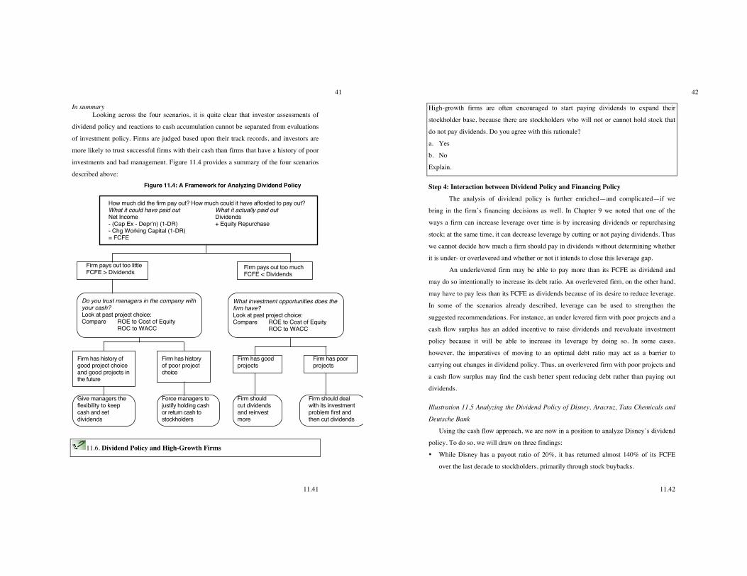
11.41

41

In summary Looking across the four scenarios, it is quite clear that investor assessments of

dividend policy and reactions to cash accumulation cannot be separated from evaluations

of investment policy. Firms are judged based upon their track records, and investors are

more likely to trust successful firms with their cash than firms that have a history of poor

investments and bad management. Figure 11.4 provides a summary of the four scenarios

described above:

How much did the firm pay out? How much could it have afforded to pay out?What it could have paid out What it actually paid outNet Income Dividends- (Cap Ex - Deprʼn) (1-DR) + Equity Repurchase- Chg Working Capital (1-DR)= FCFE

Firm pays out too littleFCFE > Dividends

Firm pays out too muchFCFE < Dividends

Do you trust managers in the company withyour cash?Look at past project choice:Compare ROE to Cost of Equity

ROC to WACC

What investment opportunities does the firm have?Look at past project choice:Compare ROE to Cost of Equity

ROC to WACC

Firm has history of good project choice and good projects in the future

Firm has historyof poor project choice

Firm has good projects

Firm has poor projects

Give managers the flexibility to keep cash and set dividends

Force managers to justify holding cash or return cash to stockholders

Firm should cut dividends and reinvest more

Firm should deal with its investment problem first and then cut dividends

Figure 11.4: A Framework for Analyzing Dividend Policy

11.6. Dividend Policy and High-Growth Firms

11.42

42

High-growth firms are often encouraged to start paying dividends to expand their

stockholder base, because there are stockholders who will not or cannot hold stock that

do not pay dividends. Do you agree with this rationale?

a. Yes

b. No

Explain.

Step 4: Interaction between Dividend Policy and Financing Policy The analysis of dividend policy is further enriched—and complicated—if we

bring in the firm’s financing decisions as well. In Chapter 9 we noted that one of the

ways a firm can increase leverage over time is by increasing dividends or repurchasing

stock; at the same time, it can decrease leverage by cutting or not paying dividends. Thus

we cannot decide how much a firm should pay in dividends without determining whether

it is under- or overlevered and whether or not it intends to close this leverage gap.

An underlevered firm may be able to pay more than its FCFE as dividend and

may do so intentionally to increase its debt ratio. An overlevered firm, on the other hand,

may have to pay less than its FCFE as dividends because of its desire to reduce leverage.

In some of the scenarios already described, leverage can be used to strengthen the

suggested recommendations. For instance, an under levered firm with poor projects and a

cash flow surplus has an added incentive to raise dividends and reevaluate investment

policy because it will be able to increase its leverage by doing so. In some cases,

however, the imperatives of moving to an optimal debt ratio may act as a barrier to

carrying out changes in dividend policy. Thus, an overlevered firm with poor projects and

a cash flow surplus may find the cash better spent reducing debt rather than paying out

dividends.

Illustration 11.5 Analyzing the Dividend Policy of Disney, Aracruz, Tata Chemicals and

Deutsche Bank

Using the cash flow approach, we are now in a position to analyze Disney’s dividend

policy. To do so, we will draw on three findings:

• While Disney has a payout ratio of 20%, it has returned almost 140% of its FCFE

over the last decade to stockholders, primarily through stock buybacks.

11.43

43

• While Disney’s project returns and stock price performance lagged in the early part of

the last decade (1999-2008), it has improved significantly on both measures in the last

four years and now delivers excess returns on both dimensions.

• Finally, in our analysis in Chapter 8, we noted that Disney was slightly underlevered,

with an actual debt ratio of 27 percent and an optimal debt ratio of between 30 and 40

percent, depending upon assumptions about operating income.

Given this combination of findings, we would recommend that Disney reduce its stock

buybacks for the near term, in the face of a slowing economy and potentially lower

earnings. If earnings stay healthy, Disney can go back to using buybacks as a way of

moving towards it optimal debt ratio. In table 11.15, we forecast the FCFE for the next 5

years, assuming that Disney funds 40% of its reinvestment needs with debt each year.

Table 11.15 Forecasted FCFE and Cash Available for Stock Buybacks: Disney (in

millions) Current 2009 2010 2011 2012 2013 Net Income $4,324 $4,540 $4,767 $5,006 $5,256 $5,519 - (Cap Ex – Depreciation) (1 – 0.40) $1,078 $1,132 $1,188 $1,248 $1,310 $1,376 - Change in Working Capital (1 - 40) $25 $27 $28 $29 $31 FCFE $3,383 $3,552 $3,730 $3,916 $4,112 Expected Dividends $697 $732 $769 $807 $847 Cash available for stock buybacks $2,686 $2,820 $2,961 $3,109 $3,265

Note that we have assumed that revenues, net income, dividends, capital expenditures

and depreciation are expected to grow 5 percent a year for the next five years and that

working capital remains at its existing percentage (2.28 percent) of revenues. Based on

these forecasts, and assuming that Disney maintains its existing dividend, Disney should

have about $14,842 million in excess cash that it can return to its stockholders in stock

buybacks over the period.

Turning our attention to Aracruz, we review our findings on the company in both

this chapter and prior ones:

• Aracruz has paid out far more in dividends than it has available in FCFE and has

funded the deficit primarily with new debt.

11.44

44

• As a result of the borrowing, Aracruz is significantly over levered, with a debt to

capital ratio in excess of 50% and an optimal debt ratio, computed in chapter 8, of

about 10%.

• While Aracruz delivered high returns between 2002 and 2007, we suspect that some

or much of these returns were the result of speculation on currency derivatives during

that period. The unraveling of this strategy in 2008 generated billions of dollars in

losses and makes us wary about management capabilities in the firm to manage risk

and deliver performance.

Taken as a whole, we see few alternatives to Aracruz other than cutting or even

eliminating dividends and using the cash to pay down debt.

With Tata Chemicals, our analysis so far has led us to the following conclusions

about the firm:

• Tata Chemicals has paid out about 70% of its FCFE as dividends each year and has

redirected the withheld cash to other companies in the Tata Group.

• While Tata Chemical’s stock price performance looks good in absolute terms, much

of that performance can be attributed to the performance of the Indian stock market.

On a risk-adjusted basis, Tata Chemicals has delivered excess returns close to zero on

both its projects and the stock.

• Tata Chemicals is over levered with a debt to capital ratio of 34% and an optimal debt

ratio of 10%, though it is not clear how much of this debt is being subsidized by the

Tata Group.

Unlike Aracruz, Tata Chemicals is not in financial distress and has some leeway to use its

dividend policy to adjust its capital structure over time. We would recommend that Tata

Chemicals continue its existing dividend policy and that it redirect some of its excess

cash to paying down debt.

Finally, with Deutsche Bank, we draw on the estimates of expected future FCFE

that we made in table 11.8. Recapping, we assumed a target regulatory capital ratio of

10% and estimated the reinvestment that would be needed in future years to sustain a

modest growth rate of 4% for the next 5 years. In table 11.16, we reproduce the expected

FCFE and net income and compute an aggregate dividend payout ratio that would be

appropriate for Deutsche Bank for the future.

11.45

45

Table 11.16: Expected FCFE and Net Income: Deutsche Bank

Year FCFE Net Income 2009 2,001 ! 3,147 ! 2010 2,114 ! 3,302 ! 2011 2,233 ! 3,463 ! 2012 2,358 ! 3,631 ! 2013 2,779 ! 3,807 !

Aggregate 11,486 ! 17,349 !

Based upon these estimates, Deutsche Bank can afford to pay out about 66% of its

earnings as dividends:

Potential Payout Ratio =

!

FCFEEarnings

=11,48617,349

= 66%

Given the uncertainties in the banking sector about potential losses on securities and

regulatory changes, we would hold off on making major changes in dividend policy until

some of the uncertainty is resolved.

A Comparable Firm Approach to Analyzing Dividend Policy So far, we have examined the dividend policy of a firm by looking at its cash

flows and the quality of its investments. There are managers who believe that their

dividend policies are judged relative to those of their competitors. This comparable-firm

approach to analyzing dividend policy is often used narrowly, by looking at only firms

that are in the same industry group or sector. As we will illustrate, it can be used more

broadly, by looking at the determinants of dividend policy across all firms in the market.

Using Firms in the Industry

In the simplest form of this approach, a firm’s dividend yield and payout are

compared to those of firms in its industry and accordingly judged to be adequate,

excessive, or inadequate. Thus, a utility stock with a dividend yield of 3.5 percent may be

criticized for paying out an inadequate dividend if utility stocks, on average, have a much

higher dividend yield. In contrast, a computer software firm that has a dividend yield of

1.0 percent may be viewed as paying too high a dividend if software firms pay a much

lower dividend on average.

11.46

46

Although comparing a firm to comparable firms on dividend yield and payout

may have some intuitive appeal, it can be misleading. First, it assumes that all firms

within the same industry group have the same net capital expenditure and working capital

needs. These assumptions may not be true if firms are in different stages of the life cycle.

Second, even if the firms are at the same stage in their life cycles, the entire industry may

have a dividend policy that is unsustainable or suboptimal. Third, it does not consider

stock buybacks as an alternative to dividends. The third criticism can be mitigated when

the approach is extended to compare cash returned to stockholders, rather than just

dividends.

There is a data set online that summarizes the dividend yields and payout ratios by

sector for U.S. companies.

Illustration 11.6 Analyzing Disney’s Dividend Payout Using Comparable Firms

In comparing Disney’s dividend policy to its peer group, we analyze the dividend

yields and payout ratios of comparable firms in 2008, as shown in Table 11.17. We

defined comparable firms as entertainment companies with a market capitalization in

excess of $500 million.

Table 11.17 Payout Ratios and Dividend Yields: Entertainment Companies Company Name Market Cap Payout Ratio Dividend Yield Astral Media Inc. 'A' $1,221.70 0.00% 0.00% CBS Corp. 'B' $5,103.70 53.52% 14.22% Central European Media Enterps $827.70 0.00% 0.00% Corus Entertainment Inc $806.50 0.00% 0.00% CTC Media Inc $715.10 0.00% 0.00% Discovery Communications Inc $3,860.60 NA 0.00% Disney (Walt) $41,114.70 17.11% 1.67% DreamWorks Animation $2,074.30 0.00% 0.00% Hearst-Argyle Television Inc $589.10 40.59% 4.46% IAC/InterActiveCorp $2,215.30 NA 0.00% Lions Gate Entertainment Corp $705.60 NA 0.00% News Corp. $23,245.30 9.07% 1.35% Regal Entertainment Group $1,447.60 176.09% 12.70% Scripps Networks $3,422.30 NA 0.00% Time Warner $34,112.40 22.17% 2.63% Viacom Inc. 'B' $10,669.30 0.00% 0.00% World Wrestling Ent. $749.50 198.45% 13.79% Average 39.77% 2.99%

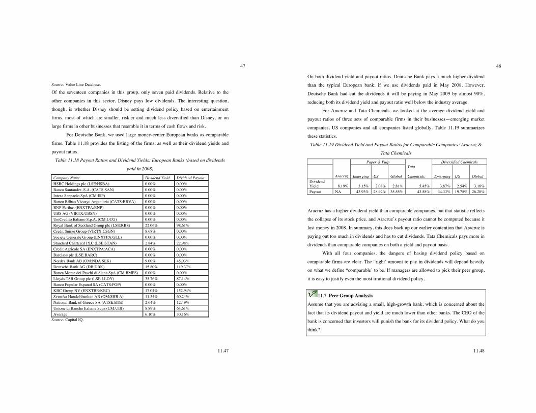
11.47

47

Source: Value Line Database.

Of the seventeen companies in this group, only seven paid dividends. Relative to the

other companies in this sector, Disney pays low dividends. The interesting question,

though, is whether Disney should be setting dividend policy based on entertainment

firms, most of which are smaller, riskier and much less diversified than Disney, or on

large firms in other businesses that resemble it in terms of cash flows and risk.

For Deutsche Bank, we used large money-center European banks as comparable

firms. Table 11.18 provides the listing of the firms, as well as their dividend yields and

payout ratios.

Table 11.18 Payout Ratios and Dividend Yields: European Banks (based on dividends

paid in 2008)

Company Name Dividend Yield Dividend Payout HSBC Holdings plc (LSE:HSBA) 0.00% 0.00% Banco Santander, S.A. (CATS:SAN) 0.00% 0.00% Intesa Sanpaolo SpA (CM:ISP) 0.00% 0.00% Banco Bilbao Vizcaya Argentaria (CATS:BBVA) 0.00% 0.00% BNP Paribas (ENXTPA:BNP) 0.00% 0.00% UBS AG (VIRTX:UBSN) 0.00% 0.00% UniCredito Italiano S.p.A. (CM:UCG) 0.00% 0.00% Royal Bank of Scotland Group plc (LSE:RBS) 22.06% 98.61% Credit Suisse Group (VIRTX:CSGN) 8.68% 0.00% Societe Generale Group (ENXTPA:GLE) 0.00% 0.00% Standard Chartered PLC (LSE:STAN) 2.84% 22.98% Credit Agricole SA (ENXTPA:ACA) 0.00% 0.00% Barclays plc (LSE:BARC) 0.00% 0.00% Nordea Bank AB (OM:NDA SEK) 9.00% 45.03% Deutsche Bank AG (DB:DBK) 15.80% 119.37% Banca Monte dei Paschi di Siena SpA (CM:BMPS) 0.00% 0.00% Lloyds TSB Group plc (LSE:LLOY) 35.76% 87.14% Banco Popular Espanol SA (CATS:POP) 0.00% 0.00% KBC Group NV (ENXTBR:KBC) 17.04% 152.94% Svenska Handelsbanken AB (OM:SHB A) 11.54% 60.24% National Bank of Greece SA (ATSE:ETE) 2.64% 12.49% Unione di Banche Italiane Scpa (CM:UBI) 8.89% 64.61% Average 6.10% 30.16%

Source: Capital IQ.

11.48

48

On both dividend yield and payout ratios, Deutsche Bank pays a much higher dividend

than the typical European bank, if we use dividends paid in May 2008. However,

Deutsche Bank had cut the dividends it will be paying in May 2009 by almost 90%,

reducing both its dividend yield and payout ratio well below the industry average.

For Aracruz and Tata Chemicals, we looked at the average dividend yield and

payout ratios of three sets of comparable firms in their businesses—emerging market

companies, US companies and all companies listed globally. Table 11.19 summarizes

these statistics.

Table 11.19 Dividend Yield and Payout Ratios for Comparable Companies: Aracruz &

Tata Chemicals

Paper & Pulp Diversified Chemicals

Aracruz Emerging US Global

Tata

Chemicals Emerging US Global Dividend Yield 8.19% 3.15% 2.08% 2.81% 5.45% 3.87% 2.54% 3.18% Payout NA 43.93% 28.92% 35.55% 43.58% 34.33% 19.75% 26.20%

Aracruz has a higher dividend yield than comparable companies, but that statistic reflects

the collapse of its stock price, and Aracruz’s payout ratio cannot be computed because it

lost money in 2008. In summary, this does back up our earlier contention that Aracruz is

paying out too much in dividends and has to cut dividends. Tata Chemicals pays more in

dividends than comparable companies on both a yield and payout basis.

With all four companies, the dangers of basing dividend policy based on

comparable firms are clear. The “right’ amount to pay in dividends will depend heavily

on what we define “comparable’ to be. If managers are allowed to pick their peer group,

it is easy to justify even the most irrational dividend policy,

11.7. Peer Group Analysis

Assume that you are advising a small, high-growth bank, which is concerned about the

fact that its dividend payout and yield are much lower than other banks. The CEO of the

bank is concerned that investors will punish the bank for its dividend policy. What do you

think?

11.49

49

a. I think that the bank will be punished for its errant dividend policy.

b. I think that investors are sophisticated enough for the bank to be treated fairly.

c. I think that the bank will not be punished for its low dividends as long as it tries to

convey information to its investors about the quality of its projects and growth

prospects.

Using the Market The alternative to using only comparable firms in the same industry is to study the

entire population of firms and try to estimate the variables that cause differences in

dividend payout across firms. We outlined some of the determinants of dividend policy in

the last chapter, and we could try to arrive at more specific measures of each of these

determinants. For instance,

• Growth Opportunities: Firms with greater growth opportunities should pay out less in

dividends than firms without these opportunities. Consequently, dividend payout

ratios (yields) and expected growth rates in earnings should be negatively correlated

with each other.

• Investment Needs: Firms with larger investment needs (capital expenditures and

working capital) should pay out less in dividends than firms without these needs.

Dividend payout ratios and yields should be lower for firms with significant capital

expenditure needs.

• Insider Holdings: As noted earlier in the chapter, firms where stockholders have less

power are more likely to hold on to cash and not pay out dividends. Hence, dividend

payout ratios and insider holdings should be negatively correlated with each other.

• Financial Leverage: Firms with high debt ratios should pay lower dividends, because

they have already precommitted their cash flows to make debt payments. Therefore,

dividend payout ratios and debt ratios should be negatively correlated with each

other.

Because there are multiple measures that can be used for each of these variables,

we chose specific proxies—analyst estimates of growth in earnings per share for growth

opportunities(EGR), percent of stock held by insiders for insider holdings (INS), and the

standard deviation in stock prices (STD) as a measure of equity risk. Using data from

11.50

50

2008, we regressed dividend yields and payout ratios against all of these variables and

arrived at the following regression equations (t-statistics are in brackets below

coefficients): PYT = 0.683 – 0.185 ROE -1.07 STD – 0.313EGR (27.41) (3.06) (10.85) (2.60)

R2 = 13.3% YLD = 0.039 – 0.039 STD – 0.010 INS – 0.093 EGR (37.38) (9.39) (2.62) (16.23)

R2 = 32.2%

The regressions explain about 32% of the differences in dividend yields and 13% of the

differences in payout ratios across firms in the United States. The two strongest factors

are earnings growth and equity risk, with higher-growth, higher-risk firms paying out less

of their earnings as dividends and having lower dividend yields. In addition, firms with

high insider holdings tend to pay out less in dividends than do firms with low insider

holdings, and firms with high capital expenditures needs seem to pay less in dividends

than firms without these needs.

There is a data set online that summarizes the results of regressing dividend yield

and payout ratio against fundamentals for U.S. companies.

Illustration 11.7 Analyzing Dividend Payout Using the Cross-Sectional Regression

To illustrate the applicability of the market regression in analyzing the dividend

policy of Disney, we estimate the values of the independent variables in the regressions

for the firm.

Insider holdings at Disney (as % of outstanding stock) = 7.70%

Standard Deviation in Disney stock prices = 19.30%

Disney’s ROE = 13.05%

Expected growth in earnings per share (Analyst estimates) = 14.50%

Substituting into the regression equations for the dividend payout ratio and dividend

yield, we estimate a predicted payout ratio:

Predicted Payout = 0.683 – 0.185 (.1305) -1.07 (.1930) – 0.313 (.145) =0.4069

Predicted Yield = 0.039 – 0.039 (.1930) – 0.010 (.077) – 0.093 (.145) = .0172

11.51

51

Based on this analysis, Disney with its dividend yield of 1.67% and a payout ratio of

approximately 20% is paying too little in dividends. This analysis, however, fails to

factor in the huge stock buybacks made by Disney over the last few years.

Managing Changes in Dividend Policy In Chapter 10, we noted the tendency on the part of investors to buy stocks with

dividend policies that meet their specific needs. Thus, at least prior to 2003, investors

who wanted high current cash flows and did not care much about the tax consequences

migrated to firms that paid high dividends; those who wanted price appreciation and were

concerned about the tax differential held stock in firms that paid low or no dividends.

One consequence of this clientele effect is that changes in dividends, even if entirely

justified by the cash flows, may not be well received by stockholders. In particular, a firm

with high dividends that cuts them drastically may find itself facing unhappy

stockholders. At the other extreme, a firm with a history of not paying dividends that

suddenly institutes a large dividend may also find that its stockholders are not pleased.

Is there a way in which firms can announce changes in dividend policy that

minimizes the negative fallout that is likely to occur? In this section, we will examine

dividend changes and the market reaction to them and draw broader lessons for all firms

that may plan to make such changes.

Empirical Evidence Firms may cut dividends for several reasons; some clearly have negative

implications for future cash flows and the current value of the firm, whereas others have

more positive implications. In particular, the value of firms that cut dividends because of

poor earnings and cash flows should drop, whereas the value of firms that cut dividends

because of a dramatic improvement in project choice should increase. At the same time,

financial markets tend to be skeptical of the latter claims, especially if the firm making

the claims reports lower earnings and has a history of poor project returns. Thus, there is

value to examining closely timed earnings and dividend cut announcements, to see if the

market reaction changes as a consequence.

11.52

52

Woolridge and Ghosh looked at 408 firms that cut dividends, and the actions

taken or information provided by these firms in conjunction with the dividend cuts.12 In

particular, they examined three groups of companies: The first group announced an

earnings decline or loss with the dividend cut; the second had made a prior announcement

of earnings decline or loss; and the third made a simultaneous announcement of growth

opportunities or higher earnings. The results are summarized in Table 11.20.

Table 11.20 Excess Returns around Dividend Cut Announcements

Periods Around Announcement Date Category Prior Quarter Announcement

Period Quarter After

Simultaneous announcement of earnings decline/loss (N = 176)

–7.23% –8.17% +1.80%

Prior announcement of earnings decline or loss (N = 208)

–7.58% –5.52% +1.07%

Simultaneous announcement of investment or growth opportunities (N = 16)

–7.69% –5.16% +8.79%

We can draw several interesting conclusions from this study. First, the vast

number of firms announcing dividend cuts did so in response to earnings declines (384)

rather than in conjunction with investment or growth opportunities (16). The market

seems to react negatively to all of them, however, suggesting that it does not attach much

credibility to the firm’s statements. The negative reaction to the dividend cut seems to

persist in the case of the firms with the earnings declines, whereas it is reversed in the

case of the firms with earnings increases or better investment opportunities.

Woolridge and Ghosh also found that firms that announced stock dividends or

stock repurchases in conjunction with the dividend cuts fared much better than firms that

did not. Finally, they noted the tendency across the entire sample for prices to correct

12J. R. Woolridge and C. Ghosh, 1986, “Dividend Cuts: Do They Always Signal Bad News?” In The Revolution in Corporate Finance. Blackwell.

11.53

53

themselves, at least partially, in the year following the dividend cut. This would suggest

that markets tend to overreact to the initial dividend cut, and the price recovery can be

attributed to the subsequent correction.

In an interesting case study, Soter, Brigham, and Evanson looked at Florida

Power & Light's dividend cut in 1994.13 FPL was the first healthy utility in the United

States to cut dividends by a significant amount (32 percent). At the same time as it cut

dividends, FPL announced that it was buying back 10 million shares over the next three

years and emphasized that dividends would be linked more directly to earnings. On the

day of the announcement, the stock price dropped 14 percent but recovered this amount

in the month after the announcement and earned a return of 23.8 percent in the year after,

significantly more than the S&P 500 over the period (11.2 percent) and other utilities

(14.2 percent).

Lessons for Firms

There are several lessons for a firm that plans to change its dividend policy. First,

no matter how good the rationale may be to cut dividends, it should expect markets to

react negatively to the initial announcement for two reasons. The first reason is the well-

founded skepticism with which markets greet any statement by the firm about dividend

cuts. A second is that large dividend changes typically make the existing investor

clientele unhappy. Although other stockholders may be happy with the new dividend

policy, the transition will take time, during which stock prices fall. Second, if a firm has

good reasons for cutting dividends, such as an increase in project availability, it will gain

at least partial protection by providing information to markets about these projects.

Dividend cuts and Investor reaction: A Behavioral Perspective

There are few corporate finance actions that managers dread more than cutting

dividends, which may explain why they happen so infrequently. When firms that are

paying too much, either because earnings have dropped or investment opportunities have

13D. Soter, E. Brigham, and P. Evanson, 1996, “The Dividend Cut ‘Heard 'Round the World’: The Case of FPL,” Journal of Applied Corporate Finance, 9, 4–15. This is also a Harvard Business School case study authored by Ben Esty.

11.54

54

increased, the rationale for cutting dividends may seem simple, there are reasons why

these firms choose to put off making this decision:

a. Indiscriminate investors: There is evidence that the stock prices of firms that cut

dividends drop, at the time of the announcement, no matter what the reasons for the

action. In other words, investors seem to treat firms that cut dividends because of

operating problems (declining earnings and losses) the same way that they treat firms

that cut dividends to invest in potentially lucrative investments.

b. Stock price drift: Michaely, Thaler and Womack looked at 887 dividend omissions

between 1964 and 1987 dividends find evidence that stock prices continue to drift

downwards in the weeks after a dividend decrease.14 While some of this downward

drift can be attributed to higher risk, it is possible that some of it is due to herd

behavior on the part of investors. Boehme and Sorescu contest this conclusion by

noting that the price drift is isolated to smaller firms.15

There is, however, some good news for firms that do need to reduce dividends. Firms that

can frame dividend decreases in terms that appeal to investors may be able to overcome

the generally negative reaction from investors, at least over longer time periods. Bulan,

Subramaniam and Talan divide dividend omissions into good and bad omissions based

upon two factors.16 They find that firms that confront and deal with dividend problems

early and use the cash from dividend omissions to retire debt see their stock prices

recover more quickly than firms that allow the pain to linger and misuse the cash from

dividend omissions.

Conclusion We began this chapter by expanding our definition of cash returned to stockholder

to include stock buybacks with dividends. Firms in the United States especially have

turned to buying back stock and returning cash selectively to those investors who need it.

14 Michaely, Roni, Richard H. Thaler, and Kent L. Womack, 1995, Price reactions to dividend initiations and

omissions: overreaction or drift? Journal of Finance 50, 573-608. 15 Boehme, Rodney D., and Sorin M Sorescu, 2002, The long-run performance following dividend initiations

and resumptions: underreaction or product of chance? Journal of Finance 57, 871-900.

16 Bulan, L., N. Subramaniam and L. Tanlu, 2005, When are dividend omissions good news? Working Paper, ssrn.com.

11.55

55

With this expanded definition, we first used a cash flow–based approach to decide

whether a firm is paying too much or too little to its stockholders. To form this judgment,

we first estimate what the firm has available to pay out to its stockholders; we measure

this cash flow by looking at the cash left over after reinvestment needs have been and

debt has been serviced, and call it the free cash flow to equity. We then looked at the

quality of the firm’s projects; firms with better projects get more leeway from equity

investors to accumulate cash than firms with poor projects. We next consider the effect of

wanting to increase or decrease the debt ratio on how much cash is returned to

stockholders. Finally, we consider all three factors—the cash flow available for

stockholders, the returns on existing investments, and the need to increase or decrease

debt ratios—in coming up with broad conclusions about dividend policy. Firms with a

good track record in investing can pay out less in dividends than is available in cash

flows, and not face significant pressure from stockholders to pay out more. When the

managers of firms are not trusted by their stockholders to invest wisely, firms are much

more likely to face pressure to return excess cash to stockholders.

We also analyzed a firm’s dividend policy by looking at the dividend policies of

comparable firms in the business. In this approach, a firm paying out less in dividends

than comparable firms would be viewed as paying too little and one that is paying out

more would be viewed as paying too much. We used both a narrow definition of

comparable firms (firms in the same line of business) and a broader definition (all firms).

We controlled for differences in risk and growth across firms using a multiple regression.

We closed the chapter by looking at how firms that intend to change their

dividend policy can minimize the side costs of doing so. This is especially true when

firms have to reduce their dividends to meet legitimate reinvestment needs. Although the

initial reaction to the announcement of a dividend cut is likely to be negative, firms can

buffer some of the impact by providing information to markets about the investments that

they plan to accept with the funds.

Given the tax law changes, at least in the United States, in 2003, it may be time to

revisit the whole basis for dividend policy. Historically, in the United States and Western

Europe, firms have locked themselves into a dance with investors where they institute

dividends and are then committed to maintaining these dividends, in good times and in

11.56

56

bad. In fact, much of what we observe in dividend policy—from sticky dividends to the

reluctance to increase dividends in the face of good news and to cut dividends in the face

of bad news—can be traced to this commitment. This commitment has also led

companies to increasingly shift to stock buybacks as an alternative to dividends. If

dividends no longer have a tax disadvantage, it is time for firms to shift to a more flexible

dividend payout policy, where dividends reflect what they can afford to pay rather than

their historical dividends.

11.57

57

Live Case Study A Framework for Analyzing Dividends

Objective To determine whether your firm should change its dividend policy, based on

an analysis of its investment opportunities and comparable firms.

Key Questions

• How much could this firm have returned to its stockholders over the past few years?

How much did it actually return?

• Given this dividend policy and the current cash balance of this firm, would you push

the firm to change its dividend policy (return more or less cash to its owners)?

• How does this firm’s dividend policy compare to those of its peer group and to the

rest of the market?

Framework for Analysis

1. Cash Return to Stockholders

• How much has the firm paid out in dividends each year for the past few years?

• How much stock has it bought back each year for the past few years?

• Cumulatively, how much cash has been returned to stockholders each year for the

past few years?

2. Affordable Dividends

• What was the FCFE that this firm had over the last few years?

• What is the current cash balance for this firm?

3. Management Trust

• How well have the managers of the firm picked investments, historically?

(Look at the investment return section.)

• Is there any reason to believe that future investments of this firm will be

different from the historical record?

4. Changing Dividend Policy

• Given the relationship between dividends and FCFE and the trust you have in

the management of this firm, would you change this firm’s dividend policy?

5. Comparing to Sector and Market

11.58

58

• Relative to the sector to which this firm belongs, does it pay too much or too

little in dividends? (Do a regression, if necessary.)

• Relative to the rest of the firms in the market, does it pay too much or too little

in dividends? (Use the market regression, if necessary.)

Getting Information on Analyzing Dividend Policy

You can get the information that you need to estimate FCFE and returns on equity

from past financials. You will also need a beta (see risk and return section) and a debt

ratio (see risk and return section) to estimate the free cash flows to equity. Finally, you

will need stock returns for your stock and the returns on a market index over the period of

your analysis.

Online Sources of

Informationwww.stern.nyu.edu/~adamodar/cfin2E/project/data.htm.

11.59

59

Questions and Problems (In the problems below, you can use a risk premium of 5.5% and a tax rate of 40% if

either is not specified) 1. Stock buybacks really do not return cash to stockholders, because only those who sell

back stock receive the cash. Is this statement true or false? Explain.

2. Between 1988 and 2008, we saw an increase in the percent of cash returned to

stockholders in the form of dividends. Why?

3. Lube Oil, a chain of automobile service stations, reports net income of $100 million

after depreciation of $50 million. The firm has capital expenditures of $80 million, and

the noncash working capital increased from $25 to $40 million. Estimate the firm’s

FCFE, assuming that the firm is all equity financed.

4. Lube Oil, in Question 3, paid a dividend of $20 million and bought back $25 million in

stock. Estimate how much the cash balance of the firm changed during the year.

5. How would your answers to the last two questions change if you were told that Lube

Oil started the year with $120 million in debt and ended the year with $135 million?

6. Now assume that Lube Oil has a return on equity of 5 percent and a cost of equity of

10 percent. As a stockholder in Lube Oil, would you want the firm to change its dividend

policy? Why or why not?

7. Tech Products reported a net loss of $80 million for the latest financial year. In

addition, the firm reported a net capital expenditure of $70 million, and a change in

noncash working capital of $10 million. Finally, the firm had $10 million in debt at the

start of the year that it paid off during the year. Estimate the FCFE.

8. Tech Products, from Question 7, pays a dividend of $40 million. Assuming that the

firm started the period with no cash, how did it raise the funding for the dividend

payment?

11.60

60

9. New Age Telecomm is a young, high-growth telecommunications firm. It pays no

dividends, though the average dividend payout for other firms in the telecommunications

sector is 40 percent. Is New Age paying too little in dividends? Why or why not?

10. The following is a regression of dividend payout ratios on the risk and ln(market

capitalization: in millions) of chemical firms:

Dividend Payout Ratio = 0.14 + 0.05 [ln (Market Capitalization in millions)] – 0.1 (Beta)

Harman Chemicals has a market capitalization of $1.5 billion and a beta of 1.2. It pays

out 22 percent of its earnings as dividends. How does this dividend payout compare to the

industry?

11. JLChem Corporation, a chemical manufacturing firm with changing investment

opportunities, is considering a major change in dividend policy. It currently has 50

million shares outstanding and pays an annual dividend of $2 per share. The firm current

and projected income statement are provided below (in millions):

Current Projected for Next Year

EBITDA $1,200 $1,350 – Depreciation $200 $250 EBIT $1,000 $1,100 – Interest expense $200 $200 EBT $800 $900 – Taxes $320 $360 Net income $480 $540

The firm’s current capital expenditure is $500 million. It is considering five projects for

the next year:

Project Investment Beta IRR (Using

Cash Flows to

Equity)

A $190 mil 0.6 12.0%

B $200 mil 0.8 12.0%

C $200 mil 1.0 14.5%

D $200 mil 1.2 15.0%

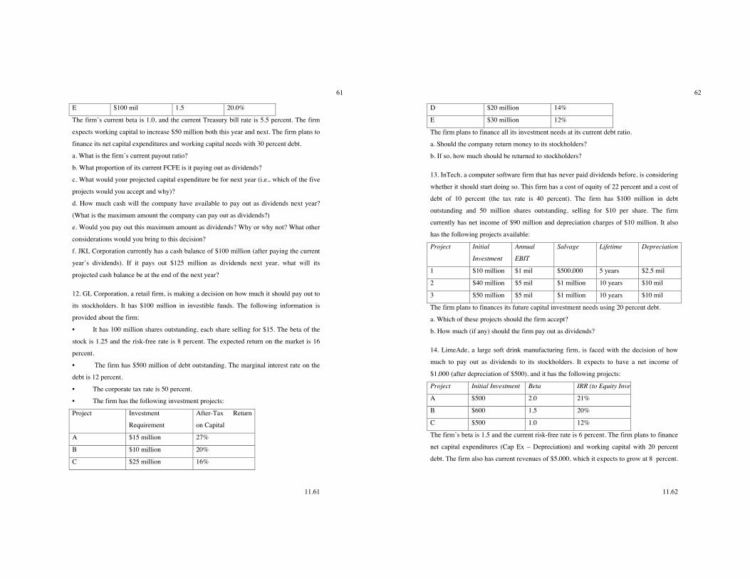
11.61

61

E $100 mil 1.5 20.0%

The firm’s current beta is 1.0, and the current Treasury bill rate is 5.5 percent. The firm

expects working capital to increase $50 million both this year and next. The firm plans to

finance its net capital expenditures and working capital needs with 30 percent debt.

a. What is the firm’s current payout ratio?

b. What proportion of its current FCFE is it paying out as dividends?

c. What would your projected capital expenditure be for next year (i.e., which of the five

projects would you accept and why)?

d. How much cash will the company have available to pay out as dividends next year?

(What is the maximum amount the company can pay out as dividends?)

e. Would you pay out this maximum amount as dividends? Why or why not? What other

considerations would you bring to this decision?

f. JKL Corporation currently has a cash balance of $100 million (after paying the current

year’s dividends). If it pays out $125 million as dividends next year, what will its

projected cash balance be at the end of the next year?

12. GL Corporation, a retail firm, is making a decision on how much it should pay out to

its stockholders. It has $100 million in investible funds. The following information is

provided about the firm:

• It has 100 million shares outstanding, each share selling for $15. The beta of the

stock is 1.25 and the risk-free rate is 8 percent. The expected return on the market is 16

percent.

• The firm has $500 million of debt outstanding. The marginal interest rate on the

debt is 12 percent.

• The corporate tax rate is 50 percent.

• The firm has the following investment projects:

Project Investment

Requirement

After-Tax Return

on Capital

A $15 million 27%

B $10 million 20%

C $25 million 16%

11.62

62

D $20 million 14%

E $30 million 12%

The firm plans to finance all its investment needs at its current debt ratio.

a. Should the company return money to its stockholders?

b. If so, how much should be returned to stockholders?

13. InTech, a computer software firm that has never paid dividends before, is considering

whether it should start doing so. This firm has a cost of equity of 22 percent and a cost of

debt of 10 percent (the tax rate is 40 percent). The firm has $100 million in debt

outstanding and 50 million shares outstanding, selling for $10 per share. The firm

currently has net income of $90 million and depreciation charges of $10 million. It also

has the following projects available:

Project Initial

Investment

Annual

EBIT

Salvage Lifetime Depreciation

1 $10 million $1 mil $500,000 5 years $2.5 mil

2 $40 million $5 mil $1 million 10 years $10 mil

3 $50 million $5 mil $1 million 10 years $10 mil

The firm plans to finances its future capital investment needs using 20 percent debt.

a. Which of these projects should the firm accept?

b. How much (if any) should the firm pay out as dividends?

14. LimeAde, a large soft drink manufacturing firm, is faced with the decision of how

much to pay out as dividends to its stockholders. It expects to have a net income of

$1,000 (after depreciation of $500), and it has the following projects:

Project Initial Investment Beta IRR (to Equity Investors)

A $500 2.0 21%

B $600 1.5 20%

C $500 1.0 12%

The firm’s beta is 1.5 and the current risk-free rate is 6 percent. The firm plans to finance

net capital expenditures (Cap Ex – Depreciation) and working capital with 20 percent

debt. The firm also has current revenues of $5,000, which it expects to grow at 8 percent.

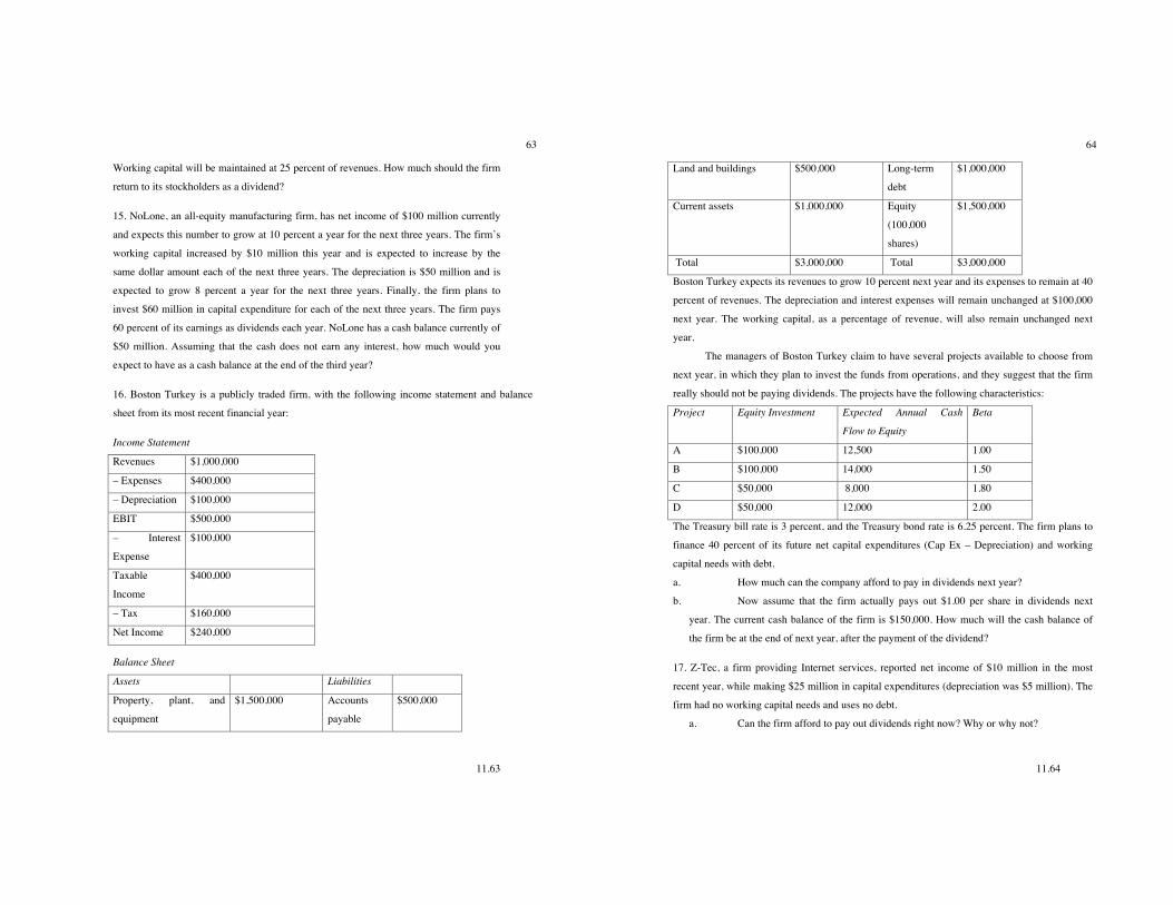
11.63

63

Working capital will be maintained at 25 percent of revenues. How much should the firm

return to its stockholders as a dividend?

15. NoLone, an all-equity manufacturing firm, has net income of $100 million currently

and expects this number to grow at 10 percent a year for the next three years. The firm’s

working capital increased by $10 million this year and is expected to increase by the

same dollar amount each of the next three years. The depreciation is $50 million and is

expected to grow 8 percent a year for the next three years. Finally, the firm plans to

invest $60 million in capital expenditure for each of the next three years. The firm pays

60 percent of its earnings as dividends each year. NoLone has a cash balance currently of

$50 million. Assuming that the cash does not earn any interest, how much would you

expect to have as a cash balance at the end of the third year?

16. Boston Turkey is a publicly traded firm, with the following income statement and balance

sheet from its most recent financial year:

Income Statement

Revenues $1,000,000

– Expenses $400,000

– Depreciation $100,000

EBIT $500,000

– Interest

Expense

$100,000

Taxable

Income

$400,000

– Tax $160,000

Net Income $240,000

Balance Sheet

Assets Liabilities

Property, plant, and

equipment

$1,500,000 Accounts

payable

$500,000

11.64

64

Land and buildings $500,000 Long-term

debt

$1,000,000

Current assets $1,000,000 Equity

(100,000

shares)

$1,500,000

Total $3,000,000 Total $3,000,000

Boston Turkey expects its revenues to grow 10 percent next year and its expenses to remain at 40

percent of revenues. The depreciation and interest expenses will remain unchanged at $100,000

next year. The working capital, as a percentage of revenue, will also remain unchanged next

year.

The managers of Boston Turkey claim to have several projects available to choose from

next year, in which they plan to invest the funds from operations, and they suggest that the firm

really should not be paying dividends. The projects have the following characteristics:

Project Equity Investment Expected Annual Cash

Flow to Equity

Beta

A $100,000 12,500 1.00

B $100,000 14,000 1.50

C $50,000 8,000 1.80

D $50,000 12,000 2.00

The Treasury bill rate is 3 percent, and the Treasury bond rate is 6.25 percent. The firm plans to

finance 40 percent of its future net capital expenditures (Cap Ex – Depreciation) and working

capital needs with debt.

a. How much can the company afford to pay in dividends next year?

b. Now assume that the firm actually pays out $1.00 per share in dividends next

year. The current cash balance of the firm is $150,000. How much will the cash balance of

the firm be at the end of next year, after the payment of the dividend?

17. Z-Tec, a firm providing Internet services, reported net income of $10 million in the most

recent year, while making $25 million in capital expenditures (depreciation was $5 million). The

firm had no working capital needs and uses no debt.

a. Can the firm afford to pay out dividends right now? Why or why not?

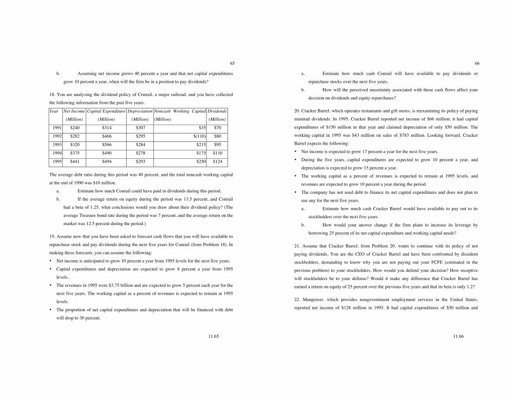
11.65

65

b. Assuming net income grows 40 percent a year and that net capital expenditures

grow 10 percent a year, when will the firm be in a position to pay dividends?

18. You are analyzing the dividend policy of Conrail, a major railroad, and you have collected

the following information from the past five years.

Year Net Income

(Million)

Capital Expenditure

(Million)

Depreciation

(Million)

Noncash Working Capital

(Million)

Dividends

(Million)

1991 $240 $314 $307 $35 $70

1992 $282 $466 $295 $(110) $80

1993 $320 $566 $284 $215 $95

1994 $375 $490 $278 $175 $110

1995 $441 $494 $293 $250 $124

The average debt ratio during this period was 40 percent, and the total noncash working capital

at the end of 1990 was $10 million.

a. Estimate how much Conrail could have paid in dividends during this period.

b. If the average return on equity during the period was 13.5 percent, and Conrail

had a beta of 1.25, what conclusions would you draw about their dividend policy? (The

average Treasure bond rate during the period was 7 percent, and the average return on the

market was 12.5 percent during the period.)

19. Assume now that you have been asked to forecast cash flows that you will have available to

repurchase stock and pay dividends during the next five years for Conrail (from Problem 18). In

making these forecasts, you can assume the following:

• Net income is anticipated to grow 10 percent a year from 1995 levels for the next five years.

• Capital expenditures and depreciation are expected to grow 8 percent a year from 1995

levels.

• The revenues in 1995 were $3.75 billion and are expected to grow 5 percent each year for the

next five years. The working capital as a percent of revenues is expected to remain at 1995

levels.

• The proportion of net capital expenditures and depreciation that will be financed with debt

will drop to 30 percent.

11.66

66

a. Estimate how much cash Conrail will have available to pay dividends or

repurchase stocks over the next five years.

b. How will the perceived uncertainty associated with these cash flows affect your

decision on dividends and equity repurchases?

20. Cracker Barrel, which operates restaurants and gift stores, is reexamining its policy of paying

minimal dividends. In 1995, Cracker Barrel reported net income of $66 million; it had capital

expenditures of $150 million in that year and claimed depreciation of only $50 million. The

working capital in 1995 was $43 million on sales of $783 million. Looking forward, Cracker

Barrel expects the following:

• Net income is expected to grow 17 percent a year for the next five years.

• During the five years, capital expenditures are expected to grow 10 percent a year, and

depreciation is expected to grow 15 percent a year.

• The working capital as a percent of revenues is expected to remain at 1995 levels, and

revenues are expected to grow 10 percent a year during the period.

• The company has not used debt to finance its net capital expenditures and does not plan to

use any for the next five years.

a. Estimate how much cash Cracker Barrel would have available to pay out to its

stockholders over the next five years.

b. How would your answer change if the firm plans to increase its leverage by

borrowing 25 percent of its net capital expenditure and working capital needs?

21. Assume that Cracker Barrel, from Problem 20, wants to continue with its policy of not

paying dividends. You are the CEO of Cracker Barrel and have been confronted by dissident

stockholders, demanding to know why you are not paying out your FCFE (estimated in the

previous problem) to your stockholders. How would you defend your decision? How receptive

will stockholders be to your defense? Would it make any difference that Cracker Barrel has

earned a return on equity of 25 percent over the previous five years and that its beta is only 1.2?

22. Manpower, which provides nongovernment employment services in the United States,

reported net income of $128 million in 1995. It had capital expenditures of $50 million and

11.67

67

depreciation of $24 million in 1995, and its working capital was $500 million (on revenues of $5

billion). The firm has a debt ratio of 10 percent and plans to maintain this debt ratio.

a. Estimate how much Manpower will have available to pay out as dividends next

year.

b. The current cash balance is $143 million. If Manpower is expected to pay $12

million in dividends next year and repurchase no stock, estimate the expected cash

balance at the end of the next year.

23. How would your answers to the previous problem change if Manpower in plans to pay off its

outstanding debt of $100 million next year and become a debt-free company?

24. You are an institutional investor and have the collected the following information on five

maritime firms to assess their dividend policies.

Company FCFE Dividends Paid ROE Beta

Alexander & Brown $55 $35 8% 0.80

American President $60 $12 14.5% 1.30

OMI –$15 $5 4.0% 1.25

Overseas Shipholding $20 $12 1.5 % 0.90

Sea Containers –$5 $8 14% 1.05

The average risk-free rate during the period was 7 percent, and the average return on the market

was 12 percent.

a. Assess which of these firms you would pressure to pay more in

dividends.

b. Which of the firms would you encourage to pay less in dividends?

c. How would you modify this analysis to reflect your expectations about

the future of the entire sector?

25. You are analyzing the dividend policy of Black and Decker, a manufacturer of tools

and appliances. The following table summarizes the dividend payout ratios, yields, and

expected growth rates of other firms in the waste disposal business.

Company Payout Ratio Dividend Yield Ex. Growth

Fedders 11% 1.2% 11.0%

11.68

68

Maytag 37% 2.8% 23.0%

National Presto 67% 4.9% 13.5%

Toro 15% 1.5% 16.5%

Whirlpool 30% 2.5% 20.5%

Black & Decker 24% 1.3% 23.0%

a. Compare Black and Decker’s dividend policy to those of its peers, using the

average dividend payout ratios and yields.

b. Do the same comparison, controlling for differences in expected growth.

26. The following regression was run using all NYSE firms in 1995

YIELD = 0.0478 – 0.0157 BETA + 0.0000008 MKTCAP + 0.006797 DBTRATIO +

0.0002 ROE – 0.09 NCEX/TA R2 = 12.88%

where BETA = beta of the stock, MKTCAP = market value of equity + book value of

debt, DBTRATIO = book value of debt/MKTCAP, ROE = return on equity in 1994, and

NCEX/TA = (capital expenditures – depreciation)/total assets. The corresponding values

for Black and Decker, in 1995, were as follows:

Beta = 1.30

MKTCAP = $5,500 million

DBTRATIO = 35%

ROE = 14.5%

NCEX/TA = 4.00%

Black and Decker had a dividend yield of 1.3 percent and a dividend payout ratio of 24

percent in 1995.

a. Estimate the dividend yield for Black and Decker, based on the regression.

b. Why might your answer be different using this approach than the answer to the

prior question, where you used only the comparable firms?

27. Handy and Harman, a leading fabricator of precious metal alloys, pays out only 23

percent of its earnings as dividends. The average dividend payout ratio for metal

fabricating firms is 45 percent. The average growth rate in earnings for the entire sector is

10 percent (Handy and Harman is expected to grow 23 percent). Should Handy and

11.69

69

Harman pay more in dividends just to get closer to the average payout ratio? Why or why

not?