Casimir Effect of Proca Fields

Quantum Field Theory Under the Influence of External Conditions

Teo Lee PengUniversity of Nottingham Malaysia Campus

18th-24th , September 2011

Casimir effect has been extensively studied for various quantum fields especially scalar fields (massless or massive) and electromagnetic fields (massless vector fields).

One of the motivations to study Casimir effect of massive quantum fields comes from extra-dimensional physics.

Using dimensional reduction, a quantum field in a higher dimensional spacetime can be decomposed into a tower of quantum fields in 4D spacetime, all except possibly one are massive quantum fields.

In [1], Barton and Dombey have studied the Casimir effect between two parallel perfectly conducting plates due to a massive vector field (Proca field).

The results have been used in [2, 3] to study the Casimir effect between two parallel perfectly conducting plates in Kaluza-Klein spacetime and Randall-Sundrum model.

In the following, we consider Casimir effect of massive vector fields between parallel plates made of real materials in a magnetodielectric background. This is a report of our work [4].

[1] G. Barton and N. Dombey, Ann. Phys. 162 (1985), 231.[2] A. Edery and V. N. Marachevsky, JHEP 0812 (2008), 035.[3] L.P. Teo, JHEP 1010 (2010), 019.[4] L.P. Teo, Phys. Rev. D 82 (2010), 105002.

From electromagnetic field to Proca field

Maxwell’s equations Proca’s equations

Continuity Equation:

(Lorentz condition)

Equations of motion for and A:

For Proca field, the gauge freedom

is lost. Therefore, there are three polarizations.

Plane waves

transversal waves

longitudinal waves

For transverse waves,

Lorentz condition

Equations of motion for A:

These have direct correspondences with Maxwell field.

Transverse waves

Type I (TE)Type II (TM)

Dispersion relation:

Longitudinal waves

Dispersion relation:

Note: The dispersion relation for the transverse waves and the longitudinal waves are different unless

Longitudinal waves

x

Boundary conditions:

and

must be continuous

must be continuous

must be continuous [5]

and

must be continuous

[5] N. Kroll, Phys. Rev. Lett. 26 (1971), 1396.

continuous

continuous

continuous

continuous

continuous

continuous

continuous continuous

Lorentz condition

Independent Set of boundary conditions:

or

are continuous

are continuous

a1a2 a3 a4

22

33

44

55

11

trt

l a

r,

r

l,

l

b,

b

Two parallel magnetodielectric plates inside a magnetodielectric medium

A five-layer model

For type I transverse modes, assume that

and are automatically continuous.

Contribution to the Casimir energy from type I transverse modes (TE)

There are no type II transverse modes or longitudinal modes that satisfy all the boundary conditions. Therefore, we have to consider their superposition.

For superposition of type II transverse modes and longitudinal modes (TM), assume that

Contribution to the Casimir energy from combination of type II transverse modes and longitudinal modes (TM):

Q, Q∞ are 4×4 matrices

In the massless limit,

one recovers the Lifshitz formula!

Special case I: A pair of perfectly conducting plates

When

It can be identified as the TE contribution to the Casimir energy of a pair of dielectric plates due to a massless electromagnetic field, where the permittivity of the dielectric plates is [2]:

0 20 40 60 80 100-14

-12

-10

-8

-6

-4

-2

0x 10

4

mass (eV)

Cas

imir

for

ce (

N)

FTECas

, nb = 1

FTMCas

, nb = 1

FCas

, nb = 1

FCasTE , n

b = 2

FCasTM, n

b = 2

FCas

, nb = 2

The dependence of the Casimir forces on the mass m when the background medium has refractive index 1 and 2. Here a = tl = tr = 10nm.

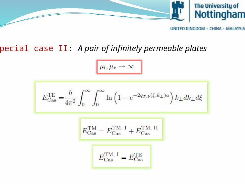
Special case II: A pair of infinitely permeable plates

It can be identified as the TE contribution to the Casimir energy of a pair of dielectric plates due to a massless electromagnetic field, where the permittivity of the dielectric plates is:

0 20 40 60 80 100-14

-12

-10

-8

-6

-4

-2

0x 10

4

mass (eV)

Cas

imir

for

ce (

N)

FCasTE , n

b = 1

FCasTM, n

b = 1

FCas

, nb = 1

FCasTE , n

b = 2

FCasTM, n

b = 2

FCas

, nb = 2

The dependence of the Casimir forces on the mass m when the background medium has refractive index 1 and 2. Here a = tl = tr = 10nm.

Special case III: One plate is perfectly conducting and one plate is infinitely permeable.

0 20 40 60 80 100-2

0

2

4

6

8

10

12x 10

4

mass (eV)

Cas

imir

for

ce (

N)

FCasTE , n

b = 1

FCasTM, n

b = 1

FCas

, nb = 1

FCasTE , n

b = 2

FCasTM, n

b = 2

FCas

, nb = 2

The dependence of the Casimir forces on the mass m when the background medium has refractive index 1 and 2. Here a = tl = tr = 10nm.

Perfectly conducting concentric spherical bodies

a3

a2

a1

Contribution to the Casimir energy from TE modes

Contribution to the Casimir energy from TM modes

The continuity of implies that in the perfectly conducting bodies, the type II transverse modes have to vanish.

In the perfectly conducting bodies,

In the vacuum separating the spherical bodies,

1 1.2 1.4 1.6 1.8 2-800

-700

-600

-500

-400

-300

-200

-100

0

100

a2/a

1

EC

asT

M/E

0

m = 0 eV

m = 10-5 eV

m = 10-4eV

1 1.2 1.4 1.6 1.8 2-1600

-1400

-1200

-1000

-800

-600

-400

-200

0

a2/a

1

EC

as/E

0

m = 0 eV

m = 10-5

eV

m = 10-4

eV

2 4 6 8 10

x 10-5

-1600

-1500

-1400

-1300

-1200

m (eV)

EC

as/E

0

a2/a

1 = 1.1

2 4 6 8 10

x 10-5

-15

-10

-5

0

m (eV)E

Cas

/E0

a2/a

1 = 1.5

THANK YOU