1 F. Properties of Continuous Random Variables F.1 The Expected Value of a Continuous Random Variable The expected value of a random variable X , denoted by µ or ( )E X is defined by

( ) ( )E f x dxX x∞

−∞

= ∫ (F.1)

Note the difference between the property (2) of a density function and the above integral. The value of the above integral is bounded by the interval where the density function is non-zero. The second raw moment of X is given by the expected value of 2( )g X X= i.e.

2 2( ) ( )E f x dX xx∞

−∞

= ∫ (F.2)

The variance of a discrete random variable is given by

2 2 2( ) ( ) ( )E X x f x dyσ µ µ∞

−∞

= − = −∫ (F.3)

which can also be simplified as

2 2 2( )E Xσ µ= − (F.3a) The expected value of a function ( )g X of a continuous random variable X is given by

( ) ( )[ ] ( ) .E f x dg X g x x∞

−∞

= ∫ .

Example F.1.1 The content of magnesium in an alloy is a random variable, given by the following pdf (probability density function)

( ) , 0 6, 18xf x x= ≤ ≤ and ( ) 0f x = elsewhere.

a. Find the expected content of magnesium. b. Find variability of the content of magnesium. c. What proportion of X values lie within σµ − and σµ + ? d. What proportion of X values lie within σµ 2− and σµ 2+ ? Solution:

a. 66 6 3

3 3

0 0 0

1 1( ) ( ) (6 0 ) 418 18 3 54x xE X x f x dx x dx

= = = = − =

∫ ∫ .

That is the mean content is 4.µ = Note 0 6.µ≤ <

2

b. 66 6 4

2 2 2 4 4

0 0 0

1 1( ) ( ) (6 0 ) 1818 18 4 72x xE X x f x dx x dx

= = = = − = ∫ ∫ .

The variance is then given by ( )22 2 2( ) 18 4 2E Xσ µ= − = − = c. which can be written as ( 5.414) ( 2.586),p P X P X= < − < which by part (c ) equals

2 2(5.414) (2.586) , 36 36

− which is 0.628.

Alternatively, one can find (2.586 5.414)P X< < by 5.414

2.5860.628.

18x dx ≈∫

d. By using part (c ), we have

( 2 2 ) (1.172 6.828),p P X P Xµ σ µ σ= − < < + ≈ < < which equals (1.172 6) (6 6.828),p P X P X= < < + < < which equals ( 6) ( 1.172) 0,p P X P X= < − < + which

equals 1 0.0381 0.962.p = − = Alternatively, one can find (1.172 6.828)P X< < by

6 6.828

1.172 60.962

180 .x dx dx+ ≈∫ ∫

Example F.1.2 Find the expected value of exponential random variable with mean 1. Solution: The density function is given by ∞<≤= − yeyf y 0 ,)( . The expected value is, therefore,

∫∫∞

−∞

==00

)( )( dyeydyyfyYE y .

Since 1

0

( ) ( 1) ( 1)yy e dyαα α α∞

− −Γ = = − Γ −∫ which is simply ( 1)!α − if α is a positive integer, it follows

that ( ) (2) 1E Y = Γ = .

Alternatively, use dyedvyu y−== , in ∫ ∫−= vduuvudv so that

0)( , , ccyedycevducedyevdydu yyyy ++=+−=+−=== −−−− ∫ ∫∫ , and consequently

0( ) ( ),y y yye d yy e c e cy c− − −= − + − + +∫ or, 01 .y

yyye dy ce

− += − −∫

Finally, we have

3

00 0 0

0

1 1( )

1 0 1 1 0 1 by L'Hosptiol's Rule

1

yy y

y yy y

y yE Y ye dy ce e

yLim Lime e e

∞ ∞∞−

→∞ →∞

+ + = = − − = − + + + = − + = − +

=

∫

Theorem F.1.1 For a non-negative random variable, ,Y we have

0( ) ( ) .E Y P Y y dy

∞= >∫

Proof. Ross (2010, 192). F.1.2 Moments For any number ,a the -tha order moment of jX is denoted by

( ) ( ) ( ) .a aa j j j jj E X x f x dxµ

∞

−∞′ = = ∫

For any integer ,a the -tha order central moment of jX is denoted by

( ) [ ( )] [ ( )] ( ) .a aa j j j j j jj E X E X x E x f x dxµ

∞

−∞= − = −∫

Moments of independently and identically distributed random variables are defined below. If a is not a non-negative integer, the expansion of [ ( )]a

j jX E X− requires some conditions. The -tha order moment of jX is given by

( ),aa E Xµ′ = or, ( ) .a

a Xx f x dxµ∞

−∞′ = ∫

Note that 1 ( )Xx f x d xµ∞

−∞′ = ∫ is often denoted by µ for simplicity.

For any integer ,a the -tha order central moment of jX is denoted by

( ) ,aa E Xµ µ= − or, ( ) ( )a

a Xx f x dxµ µ∞

−∞= −∫ where ( ) .Xx f x d xµ

∞

−∞= ∫

If a is a non-negative integer, the quantity ( )a

a E Xµ µ= − can be expanded as

0( 1) .

j a a ja a jj

aj

µ µ µ=

−=

′= −

∑

4 We refer to Stuard and Ord (1987, p.73) for further relevant formulas. In particular, we have

22 2 ,µ µ µ′= −

3

3 3 23 2 ,µ µ µ µ µ′ ′= − +

2 44 4 3 24 6 3 .µ µ µ µ µ µ µ′ ′ ′= − + −

Johnson, Kotz and Kemp (1993, 42). F.1.3 Coefficient of Skewness and Kurtosis The coefficient of skewness in a probability density function ( )f x is defined by

33( ) ( ),X E Zα = where

XZ µσ−

= and 2 2( ) .E Xσ µ= − It is popularly written as 33 3/2

2

( ) .X µαµ

=

4

4 ( ) ( ),X E Zα = where ( ) / ,Z X µ σ= − 2 2( ) .E Xσ µ= − It is popularly written as 4 22

4( ) .X µαµ

=

More generally, ( ) ( ),aa X E Zα = where

XZ µσ−

= and 2 2( ) .E Xσ µ= − It is popularly written as

/22

( ) .a

a aX µαµ

=

Johnson, Kotz and Kemp (1993, 42). F.2 Moment Generating Functions Definition F.2.1 The moment generating function ( )XM t of a discrete random variable is defined by

( )( ) ,tXXM t E e= or, ( ) ( ),tx

X XM t e f x∞

−∞= ∫ where t is continuous in the neighborhood of zero.

( )( ) ,tXX

dM t E edt

′ = or, ( ) ,tXX

dM t E edt

′ =

or, ( )( ) ,tXXM t E Xe′ = where we have assumed that the

interchange of the differentiation and integration is allowed. Hence, (0) ( ).XM E X′ =

( ) ( ),X XdM t M tdt

′′ ′= or, ( )( ) ,tXX

dM t E Xedt ′′ =

or, ( )2( ) .tXXM t E X e′′ = Hence, 2(0) ( ).XM E X′′ =

In general, ( )( ) ,n n tX

XM t E X e= 1,2,n = implying that ( )(0) ,n nXM E X= 1,2,n =

5 Example F.2.1 Determine the moment generating function of exponential random variable. Solution: The probability density function of exponential variable is given by

( ) ,Xxf x e λλ −= 0 ,x≤ < ∞ 0 ,λ≤ < ∞ and ( ) 0,Xf x = 0.x−∞ < < Since the non-zero value of the pdf

is on 0 ,x≤ < ∞ the moment generating function is

0( ) 0 ,tx x

XM t e e dxλλ∞

−= + ∫

( )

0( ) ,t x

XM t e dxλλ∞

− −= ∫

( )

0

( ) ,t x

XeM t

t

λ

λλ

∞− − = −

0 ,t λ≤ ≤

( ) ,XM tt

λλ

=−

0 ,t λ≤ ≤

Integration result: ,a

ax

x ee dx ca

= +∫ where c is a constant of integration. It disappears in definite integrals.

F.3 The Characteristic Function The characteristic function ( )XC t of a random variable X is defined by ( ) ( ),itX

XC t E e= or,

( ) ( ) ,itXX XC t e f x dx

∞

−∞= ∫ where 1.i = −

Since cos sin ,itxe tx i tx= + the above integral can be written as

( ) co s ( ) sin ( ) .X X XC t tx f x dx i tx f x dx∞ ∞

−∞ −∞= +∫ ∫

The last two integrals are well defined since the sine and cosine functions are bounded in the interval.

Because of this the characteristic function always exists.

Like the moment generating function of a random variable, the characteristic function can be used to derive

the moments of X , as stated in the following proposition.

Theorem F.3.1 Let X be a random variable and ( )XC t its cf. Let a be a positive integer. If the

-tha moment of X exists and is finite, then ( )XC t is continuously differentible a times and

0

1( ) ( ) .a

aXn a

t

dE X C ti dt

=

=

6 If a is even, the -thk moment of X exists and is finite for ;k a≤ if If a is odd, the -thk moment of

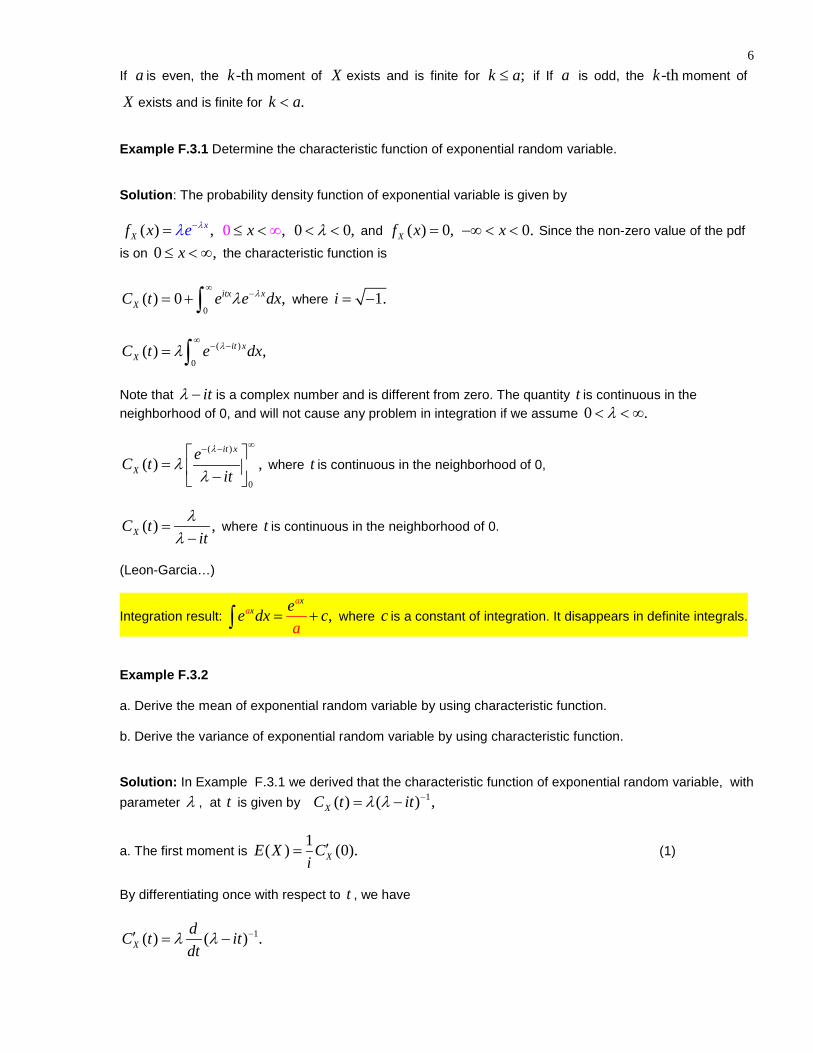
X exists and is finite for .k a< Example F.3.1 Determine the characteristic function of exponential random variable. Solution: The probability density function of exponential variable is given by

( ) ,Xxf x e λλ −= 0 ,x≤ < ∞ 0 0,λ< < and ( ) 0,Xf x = 0.x−∞ < < Since the non-zero value of the pdf

is on 0 ,x≤ < ∞ the characteristic function is

0( ) 0 ,itx x

XC t e e dxλλ∞

−= + ∫ where 1.i = −

( )

0( ) ,it x

XC t e dxλλ∞

− −= ∫

Note that itλ − is a complex number and is different from zero. The quantity t is continuous in the neighborhood of 0, and will not cause any problem in integration if we assume 0 .λ< < ∞

( )

0

( ) ,it x

XeC t

it

λ

λλ

∞− − = −

where t is continuous in the neighborhood of 0,

( ) ,XC tit

λλ

=−

where t is continuous in the neighborhood of 0.

(Leon-Garcia…)

Integration result: ,a

ax

x ee dx ca

= +∫ where c is a constant of integration. It disappears in definite integrals.

Example F.3.2 a. Derive the mean of exponential random variable by using characteristic function. b. Derive the variance of exponential random variable by using characteristic function. Solution: In Example F.3.1 we derived that the characteristic function of exponential random variable, with parameter λ , at t is given by 1( ) ( ) ,XC t itλ λ −= −

a. The first moment is 1( ) (0).XE X Ci

′= (1)

By differentiating once with respect to t , we have

1( ) ( ) .XdC t itdt

λ λ −′ = −

7

Differentiation Rule: For any fixed number ,α we have 1.dx xdx

ααα −= (3)

By using the chain rule of differentiation, we have

1 1( ) ( )( ) ,( )X

d it d itC td it dtλ λλλ

− −− −′ = ×−

2( ) ( 1)( ) [0 (1)],XC t it iλ λ −′ = − − − Then we have 2( ) ( ) .XC t i itλ λ −′ = − (4) Evaluating the above at 0t = we have

2(0) ( 0) .XiC t iλ λλ

−′ = − × =

Hence, by (1), the first moment for the exponential random variable is

1( ) .E Xλ

=

b. The variance of a variable X is defined by The quantity ( )XC t′′ is the derivative of

2( ) ( ) .XC t i itλ λ −′ = − That is

2( ) ( ) ,XdC t i itdt

λ λ −′′ = −

2 3( ) 2 ( ) .XC t i itλ λ −′′ = −

2

2

2(0) .XC iλ

′′ =

Hence by (2), we have 22 2

1 2( ) (0) .XE X Ci λ

′′= =

By (1), the variance of X is then given by

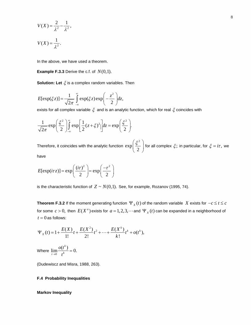
8

2 2

2 1( ) ,V Xλ λ

= −

2

1( ) .V Xλ

=

In the above, we have used a theorem. Example F.3.3 Derive the c.f. of (0,1).N Solution: Let ξ is a complex random variables. Then

21[exp( )] exp( )exp ,22zE z z dzξ ξ

π

∞

−∞

= −

∫

exists for all complex variable ξ and is an analytic function, which for real ξ coincides with

2 221 1exp exp ( ) exp .

2 2 22z dzξ ξξ

π

∞

−∞

+ = ∫

Therefore, it coincides with the analytic function 2

exp2ξ

for all complex ;ξ in particular, for ,iξ τ= we

have

2 2( )[exp( )] exp exp2 2

iE i z τ ττ −

= =

is the characteristic function of ~ (0,1).Z N See, for example, Rozanov (1995, 74). Theorem F.3.2 If the moment generating function ( )X tΨ of the random variable X exists for c t c− ≤ ≤

for some 0,c > then ( )aE X exists for 1,2,3,a = and ( )X tΨ can be expanded in a neighborhood of

0t = as follows:

22( ) ( ) ( )( ) 1 ( ),

1! 2! !

kk k

XE X E X E Xt t t t o t

kΨ = + + + + +

Where 0

( )lim 0.k

kt

o tt→

=

(Dudewiscz and Misra, 1988, 263). F.4 Probability Inequalities Markov Inequality

9 Theorem F.4.1 Let X be a nonnegative random variable ,X discrete or continuous. Then for every positive constant ,c

{ } ( ) /P X c E X c≥ ≤ Proof. For 0,c > let

1 if 0 if

X cI

X c≥

= <

Since 0,c > 1I = implies that 1 /X c≤ < ∞ which implies that 1 / ,I X c= ≤ or, / .I X c≤ Again, since

0I = implies that / 1.X c < Since 0,X ≥ and 0,c > we have 0 / 1X c≤ < which implies that 0 / 1,I X c= ≤ < or, / .I X c≤ That is in both cases, / .I X c≤

Taking mathematical expectation in both sides of the inequality, we have

( ) ( / ),E I E X c≤

1( ) ( ).E I E Xc

≤ (1)

By definition of the expected value, we have ( ) 1 ( 1) 0 ( 0),E I P I P I= = + = or,

( ) ( 1).E I P I= = By the definition of I , then, we have

( ) ( ).E I P X c= ≥ (2) From (1) and (2), we have

1( ) ( ).P X c E Xc

≥ ≤

The theorem is proved. Theorem F.4.2 Let ( )u X be a nonnegative function of the random variable ,X discrete or continuous. If

[ ( )]E u X exists, then, for every positive constant c ,

1[ ( ) ] [ ( )]P u X c E u Xc

≥ ≤ .

Proof. The proof is given when the random variable X is of the continuous type; but the proof can be adapted to the discrete case if we replace integrals by sums. Let { : ( ) }A x u x c= < ,

{ : ( ) }A x u x c′ = ≥ and let ( )f x denote the density function of .X Then

( ) ( ) ( )[ ( )] ( ) ( ) ( ) .A A

u x f x d x u x f xE dx u x f x dX xu∞

′−∞= = +∫ ∫ ∫

10 Since each of the integral in the right hand side is nonnegative, the left-hand member is at least as large as either of them. That is

( ) ( ) ( ) ( ) 0 .[ ( )]

[ ( ) ( ) ( ) ( )( .)]

A

A

E u X

E u X

u x f x dx u x f x dx

u x f x dx u x f x dx

∞

−∞

∞

′−∞

= ≥

=

≥

≥

∫ ∫∫ ∫

In particular,

( )[ ( )] ( ) ,u x f x dxE u X∞

−∞= ∫

0 + ( ) ( )

(

[ )]

A

u x f x du X xE′

≥ ∫

)[ ,( ()]

Acf x dxE u X′

≥ ∫

([ ( ] ))A

c f x dE u X x′

≥ ∫

Since, ( ) ( ) [ ( ) ],

Af x dx P X A P u X c

′′= ∈ = ≥∫ it follows that

( ) ( ) ( )[ ( )] [ ( ) ].B

u x f x dx c f x dx cP u XE u X c∞

−∞≥= ≥ ≥∫ ∫

Letting ( ) ,u X X= in TheoremG.4.2, we can prove Theorem G.4.1. Theorem F.4.3 Let the random variable X having a finite variance 2σ . Then for every 0k > ,

2

1(| | )P X kk

µ σ− ≥ ≤ ,

or equivalently, 2

1(| | ) 1 .P X kk

µ σ− < ≥ −

Proof. Put 2( ) ( )u X X µ= − and 2 2c k σ= in Theorem F.4.2. Then we have

2 22

2 222

( ) ( )

( )

1[ ] [ ],

1 1[ ] ]([ )

cc

kk

P Eu X u

P

X

X XEk

σσ

µ µ

≥ ≤

≥ ≤−≤−

Note that the assumption of finite variance implies that there is a finite mean. Example F.4.1 Let 2~ ( , ).X N µ σ Determine (| | 1.96 )P X µ σ− < by the Chebysev’s Inequality and compare it with the normal result.

11 Solution: By Chebyshev’s Inequality, we have 2(| | 1.96 ) 1 (1.96) ,P X µ σ −− < ≥ − or,

(| | 1.96 ) 0.74.P X µ σ− < ≥ But an approximate probability by the normal distribution is 0.95. Example F.4.2 Let ~ (10).X Exp Determine (| | 1.96 )P X µ σ− < by the Chebysev’s Inequality and compare it with the normal result. Solution: By Chebyshev’s Inequality, we have 2(| | 1.96 ) 1 (1.96) ,P X µ σ −− < ≥ − or,

(| | 1.96 ) 0.74.P X µ σ− < ≥ But an approximate probability by the exponential distribution is

( 1.96 1.96 ) (10 1.96(10) 10 1.96(10)),P X P Xµ σ µ σ− < < + = − < < + or,

( 1.96 1.96 ) (0 29.6),P X P Xµ σ µ σ− < < + = < < or,

( 1.96 1.96 ) 1 exp( 29.6 /10),P Xµ σ µ σ− < < + = − −

( 1.96 1.96 ) 0.9482.P Xµ σ µ σ− < < + ≈ Theorem F.4.4 Chernoff Bound ( ) ( ).ta

tP X a e M X−≥ = Leon-Garcia (2008, 183). Example F.4.3 Determine Chernoff bound for the normal distribution

Solution: 2 21( ) exp( )exp ,2

P X a ta t tµ σ ≥ ≤ − +

0 .t≤

( ) 2 21( ) exp ( ) exp ,2

P X a t a tµ σ ≥ ≤ − −

0 .t≤

( ) exp( ( )),P X a q t≥ ≤

where 2 21( ) ( ) ,2

q t t a tµ σ= − − + 0 .t≤

By minimizing the exponent, we have 2( ) / .t a µ σ= − The resulting upper bound is

21( ) exp .2

aP X a µσ

− ≥ ≤ −

This bound is better than Chebyshev bound and is similar to

2/2

2

1 1( ) ,2 (1 )

xP X x ea x a x bπ

−

≥ ≈ − + +

where 1aπ = and 2.bπ = Leon-Garcia (2008, 168). Gallager, R.G. (1968). Information Theory and Reliable Communication. Wiley.

12 F.5 Probability Distribution through Moment generating Function

Example: Let ~ (0,1).Z N Determine the moment generating function of 2W Z= and identify the distribution.

Solution: By definition, ( ) ( ),tWWM t E e= ( )2( ) exp( ) ,WM t E tZ= or,

( )2 21 1( ) exp exp ,22WM t tz z dz

π

∞

∞

= − ∫ or,

21 1( ) exp (1 2 ) .22WM t z t dz

π

∞

∞

= − − ∫

21/2 11/2

1 1 1( ) exp ,(1 2 ) 2(1 2 )2 (1 2 )WM t z dz

t ttπ

∞

−−∞

= − − −−

∫ 1/ 2.t >

The integrand may be thought of proportional to the probability density function of ( )1~ 0, (1 2 ) ,Z N t −−

for 1/ 2.t > Then

1/2

1( ) ,(1 2 )WM t

t=

− for 0.t >

The above is known to be the moment generationg function of 2~ (1),W χ so that by uniqueness theorem

of moment generating function, we conclude that 2~ (1).W χ

Inversion of Characteristic Function

Since there is a one-to-one correspondence between cumulative distribution functions and characteristic functions, it is always possible to find one of these functions if we know the other one. The formula in definition of characteristic function allows us to compute φ when we know the distribution function F (or density f). If, on the other hand, we know the characteristic function φ and want to find the corresponding distribution function, then the following inversion theorem can be used.

Theorem F.5.1 If characteristic function ( )XC t is integrable, then FX

probability density function is absolutely continuous, and

therefore X has the given by

( )Xf x =1 ( ) ,

2itx

Xe C t dtπ

∞ −

−∞∫

Galambos, Janos (1995, 113).

Example F.5.1 The characteristic function of a random variable X at t is given by ( ) 1 | |,XC t t= − for

| | 1,t ≤ and ( ) 0,XC t = for 1.t > Prove that the probability density function of the random variable is given by

2

1( ) (1 cos ),Xf x xxπ

= − .x−∞ < < ∞

13

Solution: The probability density function of X is given by 1( ) ( ) .

2itx

X Xf x e C t dtπ

∞ −

−∞= ∫ Consider

( ) .itxXI e C t dt

∞ −

−∞= ∫ It can be written as

| | 1 | | 1( ) ( ) ,itx itx

X Xt tI e C t dt e C t dt− −

≤ >= +∫ ∫ or,

| | 1 | | 1(1 | |) (0) ,itx itx

t tI e t dt e dt− −

≤ >= − +∫ ∫ or,

0 1

1 0(1 | |) (1 | |) ,itx itxI e t dt e t dt− −

−= − + −∫ ∫ or,

0 1

1 0(1 ( )) (1 ) ,itx itxI e t dt e t dt− −

−= − − + −∫ ∫ or,

0 1

1 0(1 ) (1 ) .itx itxI e t dt e t dt− −

−= + + −∫ ∫

It can be checked that ??? (imaginary number???)

( )0

21

1 1(1 ) 1 ,( )

itx ixe t dt eix ix

−

−+ = − + −∫ and

( )1

20

1 1(1 ) 1 .( )

itx ixe t dt eix ix

− −− = + −∫

Then adding the above two integrals, we have

( ) ( )2 2

1 11 1 ,( ) ( )

ix ixI e eix ix

−= − + − or,

( )2

1 2 .( )

ix ixI e eix

−= + −

Finally the probability density function is

1( )2

f xπ

= ( )2

1 2 ,( )

ix ixe eix

− + −

.x−∞ < < ∞

(G and K, 1994, 330-331.)

Example F.5.2 The characteristic function of a random variable X at t is given by ( ) exp( | |),XC t t= − for .t−∞ < < ∞ Prove that the probability density function of the random variable is given by

2

1( ) ,(1 )Xf x

xπ=

+ .x−∞ < < ∞

(K and S, 1960, 238)

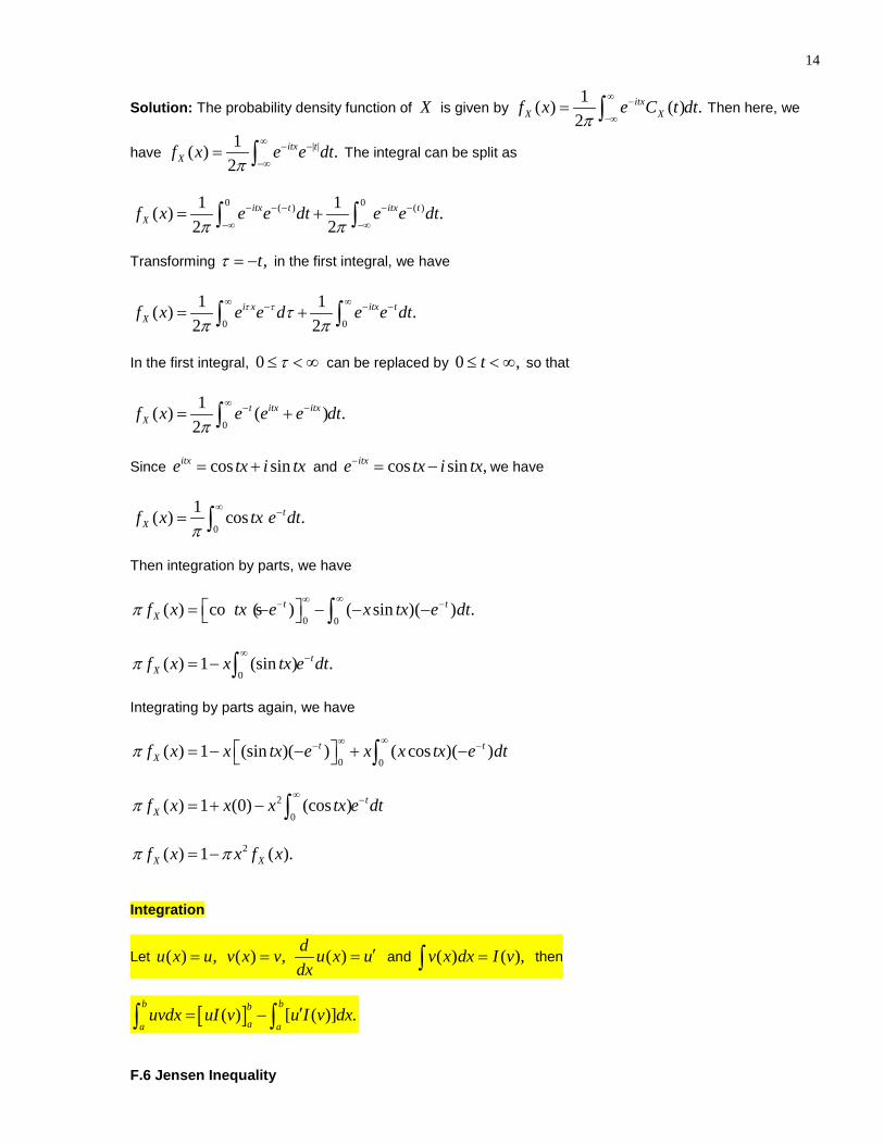
14

Solution: The probability density function of X is given by 1( ) ( ) .

2itx

X Xf x e C t dtπ

∞ −

−∞= ∫ Then here, we

have | |1( ) .2

itx tXf x e e dt

π∞ − −

−∞= ∫ The integral can be split as

0 0( ) ( )1 1( ) .

2 2itx t itx t

Xf x e e dt e e dtπ π

− − − − −

−∞ −∞= +∫ ∫

Transforming ,tτ = − in the first integral, we have

0 0

1 1( ) .2 2

i x itx tXf x e e d e e dtτ τ τ

π π∞ ∞− − −= +∫ ∫

In the first integral, 0 τ≤ < ∞ can be replaced by 0 ,t≤ < ∞ so that

0

1( ) ( ) .2

t itx itxXf x e e e dt

π∞ − −= +∫

Since cos sinitxe tx i tx= + and cos sin ,itxe tx i tx− = − we have

0

1( ) cos .tXf x tx e dt

π∞ −= ∫

Then integration by parts, we have

0 0( ) co s ( ) ( sin )( ) .t t

Xf x tx e x tx e dtπ∞∞− − = − − − − ∫

0( ) 1 (sin ) .t

Xf x x tx e dtπ∞ −= − ∫

Integrating by parts again, we have

0 0( ) 1 (sin )( ) ( cos )( )t t

Xf x x tx e x x tx e dtπ∞∞− − = − − + − ∫

2

0( ) 1 (0) (cos ) t

Xf x x x tx e dtπ∞ −= + − ∫

2( ) 1 ( ).X Xf x x f xπ π= −

Integration

Let ( ) ,u x u= ( ) ,v x v= ( )d u x udx

′= and ( ) ( ),v x dx I v=∫ then

[ ]( ) [ ( )] .b bb

aa auvdx uI v u I v dx′= −∫ ∫

F.6 Jensen Inequality

15 Convex function: A continuous function ( )g x with domain and counterdomain the real line is called

convex if for every 0x on the real line, there exists a line which goes through the point 0 0( , ( ))x g x and lies on or under the graph of the function. Theorem F.6.1 Let X be a random variable with mean ( ),E X and ( )g x be a convex function; then

( )[ ( )] ( ) .E g X g E X≥ Proof. Since ( )g x is continuous and convex, there exists a line, say ( ) ,h x a bx= + satisfying

( ) ( )h x a bx g x= + ≤ and ( ( )) ( ( )).h E X g E X= The line passes through ( ( ), ( ( )).E X g E X Also [ ( )] ( ) ( ) ( ( )).E h X E a bX a bE X h E X= + = + = Then ( ( )) ( ( )) ( ( )) ( ( ))g E X h E X E h X E g X= = ≤

Where the last step follows by the property of expected value. The theorem is known as Jensen’s inequality. It provides a lower bound of the expected value of a convex function (Mood, Graybil and Boes, 1974, 72). Alternative Proof. A function ( )g x is convex, if for any point 0 ,x the graph of ( )g x lies entirely above the

tangent at 0 ,x i.e. ( ) ( ),g x l x≥ for all ,x where ( )l x is the tangent at 0.x Hence 0 0( ) ( ).g x l x= By subtracting 0( )g x from both sides of ( ) ( ),g x l x≥ we have 0 0( ) ( ) ( ) ( ).g x g x l x g x− ≥ − Then by

virtue of 0 0( ) ( ),g x l x= we have 0 0( ) ( ) ( ) ( ).g x g x l x l x− ≥ − For any linear form of ( ),l x say,

( ) ,l x a bx= + we have 0 0( ) ( ) ( ) ( ),g x g x a bx a bx− ≥ + − + or, 0 0( ) ( ) ( ),g x g x b x x− ≥ − for all .x Replacing X for ,x and ( )E X for 0 ,x we have ( ) ( ( )) ( ( )).g X g E X b X E X− ≥ − Now taking the

expected value in both sides of the inequality, we have [ ( ) ( ( ))] [ ( ( ))],E g X g E X E b X E X− ≥ − [ ( )] [ ( ( ))] ( ) [ ( )].E g X E g E X b EX b EE X− ≥ − Since ( )E X is non-random, [ ( ( ))] ( ( )),E g E X g E X=

And [ ( )] ( ).E E X E X= Then [ ( )] ( ( )) 0.E g X g E X− ≥ This completes the proof. Theorem F.6.2 Let X be a random variable with mean ( ),E X and ( )g x be a concave function; then

( )[ ( )] ( ) .E g X g E X≤ Proof. If ( )g x is a concave function, then ( )g x− is a convex function, and by Jensen’s inequality, we have

( )[ ( )] ( ) .E g X g E X− ≥ − Multiplying both sides by 1,− we have

( )[ ( )] [ ( ) ],E g X g E X− − ≤ − − or, ( ) ( )( ) ( ) .E g X g E X≤ http://www.statlect.com/subon/inequa1.htm by Marco Taboga. It has many other cases.

In mathematics, a real-valued function ( )f x defined on an interval is called convex (or convex downward or concave upward) if the graph of the function lies below the line segment joining any two points of the graph; or more generally, any two points in a vector space. Equivalently, a function is convex if its epigraph (the set of points on or above the graph of the function) is a convex set. Well-known examples of convex functions are the quadratic function 2( )f x x= and the exponential function ( ) ,xf x e= ( ) xf x e−= for any real number x.

Convex function: To name it in terms of convexity, move towards tangent; since the movement is downward, we call the function convex downward. To name it in terms of concavity, move away from tangent; since the movement is upward, we call the function concave upward.

16 Concave function: To name it in terms of convexity, move towards tangent; since the movement is upward, we call the function convex upward. To name it in terms of concavity, move away from tangent; since the movement is downward, we call the function concave downward.

Convex function Convex downward Concave upward ( ) 0f x′′ > 2( ) ,f x x= ( ) xf x e=

Concave function Convex upward Concave downward ( ) 0f x′′ < 2( ) ,f x x= − ( ) xf x e= −

Convex functions play an important role in many areas of mathematics. They are especially important in the study of optimization problems where they are distinguished by a number of convenient properties. For instance, a (strictly) convex function on an open set has no more than one minimum. Even in infinite-dimensional spaces, under suitable additional hypotheses, convex functions continue to satisfy such properties and, as a result, they are the most well-understood functionals in the calculus of variations. In probability theory, a convex function applied to the expected value of a random variable is always less or equal to the expected value of the convex function of the random variable. This result, known as Jensen's inequality underlies many important inequalities (including, for instance, the arithmetic-geometric mean inequality and Hölder's inequality).

Exponential growth is a special case of convexity. Exponential growth narrowly means "increasing at a rate proportional to the current value", while convex growth generally means "increasing at an increasing rate (but not necessarily proportionally to current value)". (http://en.wikipedia.org/wiki/Convex_function#Properties) If the second derivative of a function is positive, the function is convex. Some examples of convex functions are given below:

a. The function 2( )f x x= has ( ) 2 0f x′′ = > at all points, so f is a convex function. It is also strongly convex (and hence strictly convex too), with strong convexity constant 2.

b. The function 4( )f x x= has 2( ) 12 0f x x′′ = ≥ , so f is a convex function. It is strictly convex, even though the second derivative is not strictly positive at all points. It is not strongly convex.

c.. The absolute value function ( ) | |f x x= is convex, even though it does not have a derivative at the point x = 0. It is not strictly convex.

d. The function ( ) | |pf x x= for 1 ≤ p is convex.

e. The exponential function ( ) xf x e= is convex. It is also strictly convex, since ( ) 0xf x e′′ = > , but it is not strongly convex since the second derivative can be arbitrarily close to zero.

f. The exponential function ( ) xf x e−= is convex. It is also strictly convex, since ( ) 0xf x e′′ = > , but it is not strongly convex since the second derivative can be arbitrarily close to zero.

Corollary Let X be a random variable and ( )g x a non-degenerate function such that ( ) 0.g x >

Then 1 1 .( ) [ ( )]

Eg X E g X

>

Kapadia, Asha S. et.al. (2005, 106-107).

17 Example F.6.2 Consider a uniform random variable ~ (0,1),X U with probability density

function ( ) 1,Xf x = for 0 1,x≤ ≤ and ( ) 0Xf x = elsewhere.

a. Derive the cumulative distribution function of ( ) .Xg X e=

b. Evaluate ( ( )).E g X

c. Determine a lower bound of ( ( ))E g X by Jensen’s Inequality, and compare with part (b).

Solution:

a. Let ( ).Y g X= Since Y is a function of ,X we denote the cumulative distribution function by ( ).YF x

Then ( ) ( ),YF x P Y x= ≤ or, ( ) ( ),XYF x P e x= ≤ or, ( ) ( ln ).YF y P X x= ≤ Since 0 1,x≤ ≤ the subset

lnX x≤ requires a condition given by 1 .x e≤ ≤ Then ln

0( ) ( ) ,

x

Y XF x f z dz= ∫ or, ( ) ln ,YF x x=

1 .x e≤ ≤

b. By differentiating ( ) ln ,YF x x= 1 ,x e≤ ≤ we have 1( ) ,Yf xx

= 1 .x e≤ ≤

The density function of Y can also be written as 1( ) ,Yf y y−= 1 .y e≤ ≤

Hence ( ) ( ),XE e E Y= or, 1

( ) ( ) ,eX

YE e yf y dy= ∫ or, 1

( ) ,eXE e dy= ∫ or, ( ) 1.XE e e= −

Ross (2010, 191).

Alternative Method:

1

0( ( )) (1) ,xE g X e dx= ∫ or, ( ( )) 1 1.71828.E g X e= − ≈

c. Since ( ) 0,g x′′ ≥ the function ( ) xg x e= is convex. Hence, by Jensen’s Inequality, we have

[ ( )] ( [ ]),E g X g E X≥ or, [ ( )] (1/ 2),E g X g≥ or, [ ( )] 1.6487.E g X e≥ ≈

http://en.wikipedia.org/wiki/Convex_function#Examples) F.7 Differential Entropy The Shannon entropy is restricted to random variables taking discrete values. The corresponding formula for a continuous random variable with probability density function ( )Xf x on the real line is defined by analogy, using the above form of the entropy as an expectation:

( ) ( ) ln ( ).X XH f f x f x∞

−∞= −∫

A precursor of the continuous entropy H(f) is the expression for the functional H in the H-theorem of Boltzmann. Example F.7.1 Determine the differential entropy for the standard normal distribution.

18

Solution: ( )ln 2 4.13.eπ ≈

F.8 Distribution of a function of a Random Variable Write introduction from Hogg and Craig (1978, 132). Cumulative Distribution Function Method Theorem F.8.1 Let X be a continuous random variable having probability density function ( ),Xf x and

cumulative distribution function ( ) ( ) .t x

X XtF x f t dt

=

=−∞= ∫ Then ( ) ( ).X X

df x F xdx

=

Example F.8.1 Let X be uniformly distributed over (0,1). Derive the cumulative distribution function of

nY X= and differentiate to derive probability density function of ,nY X= 0.n > Solution: ( ) ( ),YF y P Y y= ≤ or, ( ) ( ),n

YF y P X y= ≤ or, 1/( ) ( ),nYF y P X y= ≤ or, 1/( ) ( ),n

Y XF y F y=

or, 1/( ) ,nYF y y= for 0,n > 0 1.y≤ ≤ Then by differentiating with respect to ,y we have

(1/ ) 11( ) (1) ,n

Yf y yn

−= for 0,n > 0 1.y≤ ≤

( ) 0,Yf y = elsewhere. Transformation Method Theorem F.8.2 Let X be a continuous random variable having probability density function ( ).Xf x

Suppose that ( )y g x= is a strictly monotonic (increasing or decreasing), differentiable function of .x Then the random variable ( )Y g X= has the following probability density function

1 1( ) ( ( )) ( ) ,Y Xdf y f g y g ydy

− −= if ( )y g x= for some ;x

( ) 0,Yf y = if ( )y g x≠ for all .x

Proof. (Kapadia, Asha S. 2005, 111-112) Example F.8.2 Let X be uniformly distributed over (0,1). Derive the probability density function of

,nY X= 0.n ≠ Solution: The probability density function of X is given by ( ) 1,Xf x = for 0 1,x≤ ≤ and

( ) 0,Xf x = elsewhere. Let ( ) ny g x x= = so that 1 1/( ) .ng y y− = Then 1 1/( ( )) ( ),n

X Xf g y f y− = or, 1 1/( ( )) ( ),nX Xf g y f y− = or,

1( ( )) 1,Xf g y− = 0 1.y≤ ≤

19

Also 1 1/ (1/ ) 11( ) ,n nd dg y y ydy dy n

− −= = 0.n >

Then by Theorem F.8.2, we have

(1/ ) 11( ) (1) ,nYf y y

n−= for 0,n ≠ 0 1.y≤ ≤

( ) 0,Yf y = elsewhere.

Example F.8.3 Let X be a continuous random variable with probability density function ( ).Xf x Derive the

cumulative distribution function of 2Y X= and differentiate to derive probability density function of 2.Y X=

Solution: ( ) ( ),YF y P Y y= ≤ or, 2( ) ( ),YF y P X y= ≤ or, ( ) ( ),YF y P y X y= − ≤ ≤ or,

( ) ( ) ( ).Y X XF y F y F y= − − Then by differentiating with respect to ,y we have

( ) ( )1( ) .2Y X Xf y f y f y

y = + −

Example F.8.3 Let 2~ ( , )X N µ σ with probability density function ( ).Xf x Use the previous example to

derive probability density function of 2.Y X= Solution: From the previous example, we have

( ) ( )1( ) .2Y X Xf y f y f y

y = + −

Since the probability density function of X is given by

21 1( ) exp ,22Xf x x

π = −

,x−∞ < < ∞

we have

1 1 1( ) exp exp ,2 22 2 2Yy yf y

y π π = − + −

1 1( ) exp ,

22Yyf y

yπ = −

0 .y≤ < ∞

This is the probability density function of 2~Y χ random variable with 1 degrees of freedom.

20 Example F.8.4 Let X be a random variable of the continuous type, having the probability density function

( ) 2 ,Xf x x= 0 1,x≤ ≤ and ( ) 0,Xf x = elsewhere. Derive the distribution of 24 .Y x= Solution: The space A of x where ( ) 0Xf x > is given by { : 0 1}.xA x x= ≤ ≤ Under the transformation

24y x= , the set A maps on to { : 0 4}yB y y= ≤ ≤ and moreover the transformation is one to one. For

every 0 4a b≤ < ≤ , the event a Y b≤ ≤ will iff, the event 1 12 2

a X b≤ ≤ occurs because there is a

one to one correspondence between the points in xA and .yB Thus, we have

1 1( ) ,2 2

P a Y b P a X b ≤ ≤ = ≤ ≤

or,

12

12

( ) 2 .b

aP a Y b xdx≤ ≤ = ∫

Rewriting this integral by the transformation 24y x= , we have

( ) ,4

b

a

dyP a Y b yy

≤ ≤ =

∫ or,

1( ) .4

b

aP a Y b dy≤ ≤ = ∫

Since this is true for every 0 4,a b≤ < ≤ the probability density function of Y is the integrand; that is

1( ) ,4Yf y = 0 4.y≤ ≤

Note that

1 1( ) ,2 2Y X

df y f y ydy

=

0 4.y≤ ≤

Distribution of the Distribution Function G and K, Casella and Berger F.9 Hazard Rate Function

21 Definition F.9.1 Let X a positive continuous random variable with probability density function ( )Xf x

and cumulative distribution function ( ).XF x The hazard rate (failure rate) ( )tλ of F is defined by

( )( ) .1 ( )

X

X

f ttF t

λ =−

Example F.9.1 The hazard rate function of exponential distribution with mean 1/ λ is given by .λ F.10 The Mean and Quantile Inequality The following lemma is well known . Lemma F.10.1 If X is a nonnegative random variable, then

0

( ) (1 ( ))E X F x dx∞

= −∫

where ( )F x is the cumulative distribution function (cdf) of X . Lemma F.10.2 Let G be a nonnegative decreasing function on [0, )∞ . Then

0

( ) ( ) .x

xG x G t dt≤ ∫

Proof. Since ( ) ( )G x G t≤ for all 0 t x≤ ≤ , ( )G x is (Riemann) integrable on each interval [0, ]x for 0x > and then it follows that

0 0

( ) ( ) ( )x x

G t dt G x dt xG x≥ =∫ ∫ for all 0x ≥ .

Theorem F.10.1 Let ( )F x be the cdf of a nonnegative continuous random variable X . Then /px pµ≤

for each (0 1)p p< < such that ( ) 1 .pF x p= − Proof. Since the function ( ) 1 ( )G x F x= − is decreasing on [0, )∞ and nonnegative, by Lemma F.10.1 and Lemma F.10.2, we have the following for all 0x ≥ :

0

( ) ( ).G t dt xG xµ∞

= ≥∫

Hence for each (0,1)p ∈ , if we denote by px , the real number x such that ( ) 1 ,F x p= − we have

( )pG x p= and hence .ppxµ ≥ It is worth noting that in case 1/ 2p = , it follows from Theorem F.10.1 that 2µ µ≤ where 0.5xµ = , the

median of X . Let X be a random variable with mean µ and standard deviation σ . For 0 1p< < , the p th quantile

xp of X is defined by ( ) P X x pp≤ ≥ and ( ) 1P X x pp≥ ≥ − or equivalently

( ) ( )P X x p P X xp p< ≤ ≤ ≤ (Rohatji, 1984, 164). For example if 2/1=p , then xp µ= , the

median of the random variable X . Page and Murty (1982 and 1983) published an elementary proof of the

22 inequality | | µ µ σ− ≤ . O’Cinneide (1990) presented a new proof for | | µ µ σ− ≤ and stated the following generalization. Proposition F.10.1 Let X be a random variable with mean µ and standard deviation σ . Then for

10 << p and pq −= 1 , the following inequality holds

( )| | max / , /x p q q pp µ σ− ≤ where xp is the p th quantile.

For 2/1=p , it follows from the above proposition that | | µ µ σ− ≤ . Dharmadhikari (1991) noted that for 2/1≠p , the inequality is somewhat unsatisfactory. The refined inequality proved by her with the help of one-sided Chebyshev inequality is stated in the following theorem. Proposition F.10.2 Let X be a random variable with mean µ and standard deviation σ . Then for

10 << p and pq −= 1 , the following inequalities hold

/ / .q p x q ppµ σ µ σ− ≤ ≤ +

For stimulating discussions, readers may go through Mallows (1991) and the references therein. A more general inequality than that in Proposition 1.2 relating sample standard deviation to mean and the i -th order statistic discussed by David (1988 and 1991) is presented in Theorem 1.2. Interested readers can go through the references in David (1988) for bounds of order statistics. 11. Creating Skewed Distribution Farnandez and Steel (1998) have devised a clever way for inducing skewness in symmetric distributions such as normal and t-distributions. See for example, Ruppert, David (2011). S References Ruppert, David (2011). Statistics and Data Analysis for Financial Engineering. Springer. Fernandez, C. and Steel, M.F.J. (1998). On Bayesian modelling of fat tailes and skewness. Journal of the American Statistical association, 93, 359-371. Tutorial F.1 Consider a popular probability density function. a. Write out the probability density function. Check that the function integrates to 1.

b. Consider the identity ( ) 1,Xf x dx∞

−∞=∫ in some parameters. Differentiate the identity with respect to

every parameter 4 times and simplify to have 4 new identities. c. Determine the factorial moments. d. Determine the raw moments. e. Determine the mean centered moments. f. Determine the coefficient of skewness and kurtosis.

23 g.. Determine the moment generating function. h. Determine the characteristic function. i. Derive the moment generating function 4 times.

Essential Problems F.2 A box is to be constructed so that its height is 5 inches and its bases Y inches by Y inches , where Y is a random variable described by

( ) 6 (1 ), 0 1.f y y y y= − < < a. Find the expected value of 25 Y . b. Explain the quantity you found in part (a). (Larsen, Richard and Marx, Morris L. , 2001, 213). Partial Solution:

a. 12

0(5 ) {6 (1 )} 1.5.E Y y y y dy= − =∫ (b) The expected volume.

F.3 The probability that a baker will have sold all of his loaves X hours after baking is given by the pdf

( )236 , 0 6( )

0 elsewhere

k x xf x

− ≤ ≤=

Calculate the mean number of hours by which the baker sells all his loaves.(Brayars, 1983, 125) F.4 The length X of an offcut of wooden planking is a random variable which can take any value up to 0.5 m. It is known that the probability of the length being not more than x m (0 0.5)x≤ ≤ is kx . a. What is the expected length of X ? b. What is the standard deviation of X ? (Bryars, 1983, 127) (Ans: a. 0.25m, b. 0.144 m) F.5 Petrol is delivered to garage every Monday morning. At this garage the weekly demand for petrol, in thousands of units, is a continuous random variable X with pdf

( ), 0 1( )

0 elsewhereax b x x

f x− ≤ ≤

=

a. Given that the mean weekly demand is 600 units, determine the values of and a b . b. If the storage tanks at this garage are filled to their total capacity of 900 units every Monady morning, what is the probability that in any given week the garage will be unable to meet the demand for petrol? (Bryars, 1983, 127) (Ans: (a) 12/5, 3/2 (b) 0.125)

24 F.6 The lifetime X in years of an electric light bulb has the pdf

(5 ), 0 5( )

0 elsewherecx x x

f x− ≤ ≤

=

a. Show that 6 /125c = b. Find the mean lifetime of the bulb. c. Given that a lamp standard is fitted with two such new bulbs and their failures are independent, find the probability that neither bulb fails in the first year. d. Given that a lamp standard is fitted with two such new bulbs and their failures are independent, find the probability that exactly one of the two bulbs fails within two year. (Bryars, 1983, 128) (b) 5/2 , (c) 0.803, (d) 0.456 F.8 If the amount of cosmic radiation to which a person is exposed while flying by jet across the US is a random variable having the normal distribution with mean 4.35 mrem and standard deviation 0.59 mrem, find the probability that the amount of cosmic radiation to which a person will be exposed on such a flight is at least 5.50 mrem. ( Miller, Irwin et. Al. ,1990, 145) F.9 Find the mean of the time to failure random variable possessing the density function

4( ) ( 1) , 0f y k y y−= + ≤ (Dougherty, 1990, 305) where k is the normalizing constant. Partial Solution: ( 1) 3 / 2E y + = F.10 Prove that 2( ) , 1f y y y−= ≤ is a valid pdf. a. Prove that the mean of the distribution is not finite. b. Find the median of the distribution. (Larsen and Marx, 2001, 200) Ans. b. 0.5 2y = F.11 Consider the pdf defined by 3( ) 2 , 1f y y y−= ≤ . Calculate variance of the distribution. (Larsen and Marx, 2001, 200) F.12 Certain coded measurements of the pitch diameter of threads of a fitting have the pdf (probability density function )

2

4 , 0 1(1 )( )

0, otherwise

xxf x π

< < +=

a. Check if the above is a pdf. b. Find the probability that the coded measurements vary between 0.25 to 0.75. c. Find the variance of the coded measurements. Partial Ans (c ) 2 ( ) ln 2E X = . Advanced Problems F.13 An engineer designed a ball whose radius r changes from 10 inches to 20 inches with pdf given by

25

1 21500 (225 (3 45) ),10 20( )

0, otherwiser r

f r− − − ≤ ≤

=

a. Sketch the function ( )f r b. What proportion of balls have radius more than 15 inches? c. What is the expected radius of the balls? d. Find the expected surface area ( )S of the balls. e. Find the expected volume ( )V of the balls?

Partial Solution. 26 9 3( )5 50 500

f r r r= − + − , ( )3 45000 11600 63000 3600E R = − + − = ,

24S rπ= , 3 34 ( ) 4800 in3

V E Rπ π= =

F.14 A random variable Y , which represent the weight (in ounces) of an article, has probability density function given by

8 8 9

( ) 10 9 100

y for yf y y for y

otherwise

− ≤ ≤= − < ≤

a. Calculate the mean of the random variable Y . b. What is the probability that the weight of an article is more than 8.25 ounces? c. The manufacture sells the article for a fixed price of $2.00. He guarantees to refund the purchase money to any customer who finds the weight of his article to be less than 8.25 ounces. His cost of production is related to the weight of the article by the relation ( /15) 0.35Y + . Find the expected profit per article. Partial Solution: a. 9 b. 0.969 approx. c. The sale price of the article is given by 2 for 8.25X ≥ and 0 for 8.25X < . The profit (sale price – cost) is given by

0 [( /15) 0.35] if 8.252 [( /15) 0.35] if 8.25

Y XZ

Y X− + <

= − + ≥

F.15 The pH of a reactant is measured by the random variable X whose density function is given by

25( 3.8) if 3.8 4( ) 25( 4.2) if 4 4.2

0 elsewhere

x xf x x x

− ≤ ≤= − − ≤ ≤

a. What is the median pH of the reactant b. What is the probability that the pH of the reactant exceeds 3.9?

Hints: (a) ( 4) 1/ 2P X ≤ = (b) ( 3.9) 1 ( 3.9) 0.875P X P X> = − ≤ =

26

Mathematical Problems F.16 Find the expected value of exponential random variable with mean 1.

F.17 Consider the gamma probability function 1( )( ) .

( )

x

Xx ef x

α λλ λα

− −

=Γ

Prove that 2 2( ) ( 1) /E X α α λ= +

and 2( ) / .Var X α λ= F.18 Let X be a continuous random variable with probability density function

1( )2

f xπ

= ( )2

1 2 ,( )

ix ixe eix

− + −

.x−∞ < < ∞

a. Show that the above probability function can be expressed as the following:

2

1 cos( ) ,xf xxπ

−= .x−∞ < < ∞

b. Derive the characteristic function of the above probability density function. F.19 Let X be uniformly distributed over (0,1). a. Derive the cumulative distribution function of 3Y X= and differentiate to derive probability density function of 3.Y X= Draw the probability function. b. Prove that the mean and variance of Y are given by 1/4 and 9/112 respectively. F.20 Let X be a continuous random variable with probability density function

2

2 2

1( ) exp ,2Xxf x x

σ σ

= −

0 ,x≤ < ∞ and ( ) 0Xf x = elsewhere.

a. Prove that the cumulative probability function of XY e= is given by

( ) (ln ).Y XF y F y= b. Simplify the cumulative probability function in part (a).

c. Prove that 1(ln ) (ln ).X X

d F y f ydy y

=

d. Determine the probability density function of ( ) .Xg X e=

e. Evaluate (e ).XE

f. Determine a lower bound of (e )XE and compare with part (c).

27

g. Evaluate that that 1 1 .

2E

Xπ

σ =

h. Evaluate that ( ) .2

E X πσ=

i. Prove that 2W X= is an exponential random variable with mean 22 .σ

i. Prove that ( )( ) exp / 2 .XE e σ π≥

j. Prove that ( )(ln ) ln / 2 .E X σ π≤

k. Prove that ( ) .2

P X πσ≥ ≤

Kapadia, Asha S. et.al. (2005, 113). F.21 Let X be a continuous random variable with probability density function

2

2 2

2( ) exp ,Xxf x x

σ σ

= −

0 ,x≤ < ∞ and ( ) 0Xf x = elsewhere.

a. Prove that the cumulative probability function of XY e= is given by

( ) (ln ).Y XF y F y= b. Simplify the cumulative probability function in part (a).

c. Prove that 1(ln ) (ln ).X X

d F y f ydy y

=

d. Determine the probability density function of ( ) .Xg X e=

e. Evaluate (e ).XE

f. Determine a lower bound of (e )XE and compare with part (c).

g. Evaluate ( ),E X 1 ,EX

(ln )E X and ( ).XE e

k. Find an upper bound of ( ).P X σ≥

l. Prove that ( ) .tXE e I=

where ( )0exp .I t u u du

∞= −∫

j. Substitute 2tv u= − to prove that ( )

22

1/ 22exp exp ,

4 2t tI v v dv

∞ = − +

∫

k. Prove that 2

1/ 4 1 1exp 14 2 2tI e t πε− = + −

28

where ( ) ( )2

0

2 exp ,y

y t duεπ

= −∫ is the error function.

l. Prove that 22

1exp( ) ,1

E tXtσ

= −1| | .tσ

<

F.22 Let X be a continuous random variable with probability density function

( )( ) exp ,Xf x kx xτ α= − 0 ,x≤ < ∞ 0 ,α< < ∞ 0 ,τ< < ∞ and ( ) 0Xf x = elsewhere.

Determine the constant .k F.23 Suppose that W is an exponential random variable with mean 22 .σ Prove that X W= has The following probability function:

2

2 2

1( ) exp ,2Xxf x x

σ σ

= −

0 ,x≤ < ∞ and ( ) 0Xf x = elsewhere.

F.24 Let ~ ( / 2, / 2 ).X U π π− Prove that tanY X= has the following probability function:

2

1( ) ,(1 )Yf y

yπ=

+ .y−∞ < < ∞

F.25 Consider the probability function

| |( ) exp ,Xxf x θθ

− − =

.x−∞ < < ∞

a. Prove that the moment generating function ( )XM t of X can be expressed as

21 12 ( ) exp exp .XeM t t x dx e t x dxθ

θθ

θ θ∞

−∞

= + + − ∫ ∫

b. Prove that the moment generating function ( )XM t of X can be expressed as

2 2(1 ) ( ) .t

Xt M t eθθ− = c. Prove that the moment generating function ( )XM t of X can be expressed as

2

2( ) 1 32!XtM t tθ θ= + + +

and that mean and variance are given by θ and 22θ respectively. (K and S, 1960, 236). F.26 Let X be a continuous random variable with probability density function

29

( )( ) exp ,(1/ )Xf x xαα

α= −Γ

0 ,x≤ < ∞ 0 ,α< < ∞ and ( ) 0Xf x = elsewhere.

Check if the above is a pdf. F.27 Let X be a continuous random variable with probability density function

( )( ) exp ,Xf x kx xτ α= − 0 ,x≤ < ∞ 0 ,α< < ∞ 0 ,τ< < ∞ and ( ) 0Xf x = elsewhere.

Determine the constant .k F.28 Let 1 2, , nX X X be independently and identically distributed normal variables with unknown mean

µ and known variance 2.σ Evaluate that the Fisher Information 2

2( ) ln ( ) ,dI E Ld

µ µµ

= −

for the unknown parameter ,µ is given by 2/ .n σ Note that ( )L µ is the joint density function of the sample treated as a function of parameter .µ References Taboga, Marco (2012). Lectures on Probability Theory and Mathematical Statistics. e/2 Kapadia, Asha S. et.al. (2005). Mathematical Statistics with Applications. Chapman and Hall / CRC Press Kapur, J.N. and Saxena, H.C. (1960). S. Chand and Company Ltd, New Delhi, India. Datta, Gauri S. and Sarker, Sanat K. (2008). A general proof of some known results of independence between two statistics, TAS, 62(2), 141-143. Paulo, Aureo De (2008). Conditional moments and independence, TAS, 62(2), 219-221.

30

F.1 ( ) ( ) .E X x f x dxµ∞

−∞

≡ = ∫

F.2 2 2 2 2 2( ) ( ) , ( ) ( ) .E X x f x d x V X E Xσ µ∞

−∞

= ≡ = −∫

F.3 ( ) ( ) , a aE X x f x dx∞

−∞

= ∫

F.4 ( ) ( ) ( ) , a aa E X x f x dxµ µ µ

∞

−∞

′ ≡ − = −∫