Chapter 8

Correlation

Correlation Analysis

So far we have done statistics for one variable. In the following chapters, we will study how to relate two variables.

The knowledge of the relationship between two variables will help us to answer questions like

• Does blood pressure level predict life expectancy?

• Do SAT scores predict college performance?

• Does knowing a father’s height help predict his son’s height?

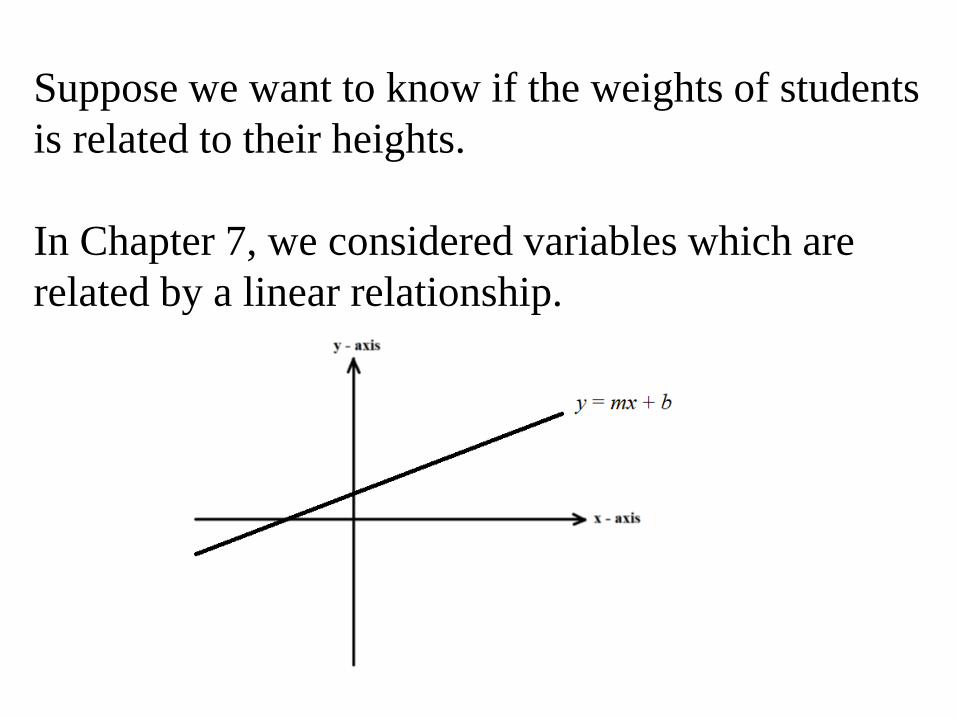
Suppose we want to know if the weights of students is related to their heights.

In Chapter 7, we considered variables which are related by a linear relationship.

In statistics, things never are so clean!

We know that height has an influence on weight – but it’s not the sole influence.

There are other factors like gender, age, body type, and random variation that influence the height.

Because of other factors, the relationship looks more like this.

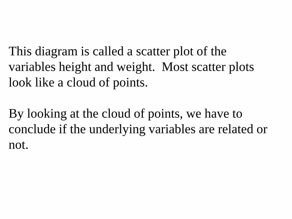
This diagram is called a scatter plot of the variables height and weight. Most scatter plots look like a cloud of points.

By looking at the cloud of points, we have to conclude if the underlying variables are related or not.

In statistics, we summarize the cloud of points by five numbers. Four of these numbers are the average of the x-values, the SD of the x-values, the average of the y-values, and the SD of the y-values.

But we need a fifth number called the correlation coefficient. It is denoted by r.

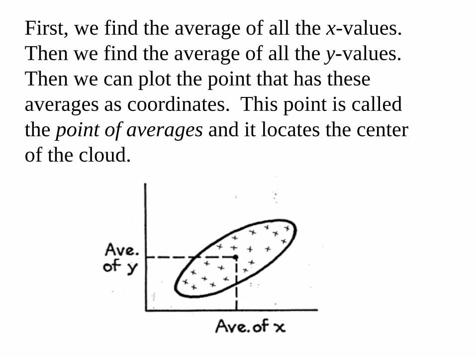
First, we find the average of all the x-values. Then we find the average of all the y-values. Then we can plot the point that has these averages as coordinates. This point is called the point of averages and it locates the center of the cloud.

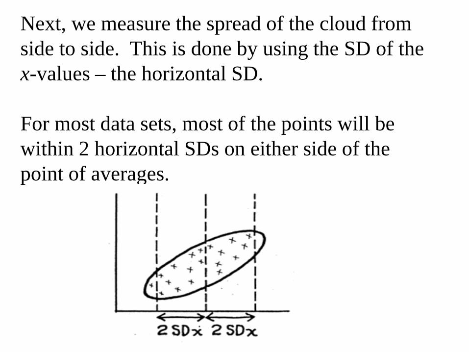
Next, we measure the spread of the cloud from side to side. This is done by using the SD of thex-values – the horizontal SD.

For most data sets, most of the points will be within 2 horizontal SDs on either side of the point of averages.

In the same way, the SD of the y-values – the vertical SD – can be used to measure the spread of the cloud from top to bottom.

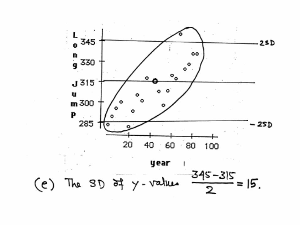
The following scatter plot shows that the performance in the long jump in the Olympic games from 1900 to 1984. By examining this scatter plot answer (approximately) the following questions.

(a) What is the point of averages of this plot?

(b) Approximately, what is the average of the x-values?

(c) Approximately, what is the SD of the x-values?

(d) Approximately, what is the average of the y-values?

(e) Approximately, what is the SD of the y-values?

Let’s see why we need the correlation coefficient.

Say we observe the data

(1,5), (1,3), (1,5), (1,7), (2,3), (2,3), (2,1), (3,1), (3,1), (4,1)

It is not enough just to find

ave of x-values = 2SD of x-values = 1ave of y-values = 3SD of y-values = 2

because these numbers give no information about the relationship between the x’s and y’s. Many other data sets may have these same descriptive statistics, but may look very different. For instance, consider the following data set which has the same x- and y- values.

Say we observe the data

(1,1), (1,1), (1,1), (1,1), (2,3), (2,3), (2,3), (3,5), (3,5), (4,7)

Here the individual descriptive statistics for the two variables are also

ave of x-values = 2SD of x-values = 1ave of y-values = 3SD of y-values = 2

since the x and y values are the same. However, it is clear that the relationship between the variables are quite different in the two data sets.

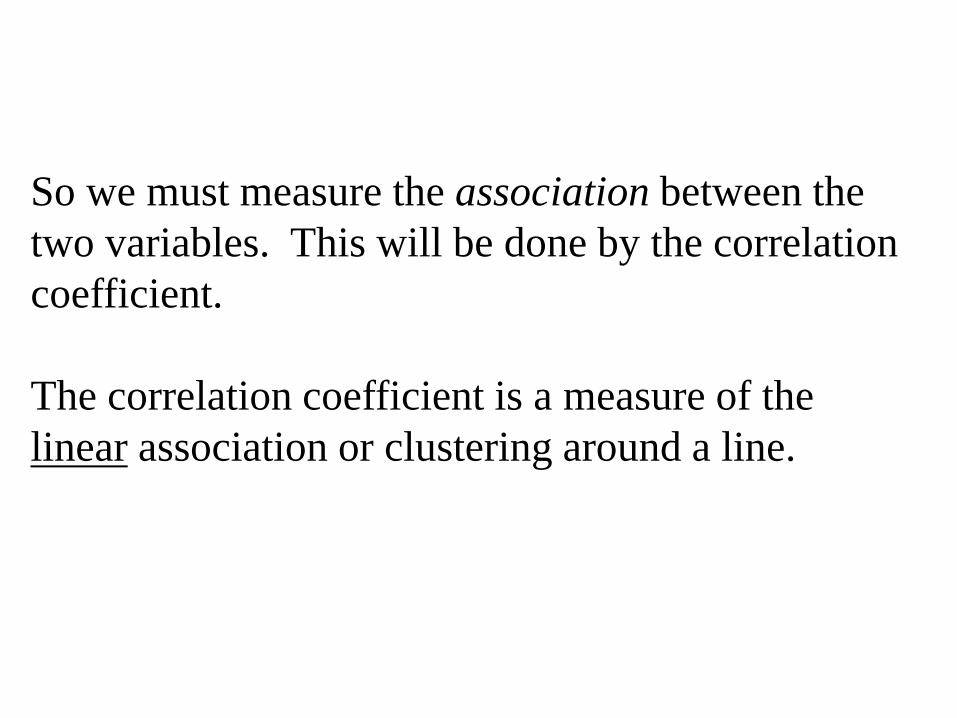
So we must measure the association between the two variables. This will be done by the correlationcoefficient.

The correlation coefficient is a measure of the linear association or clustering around a line.

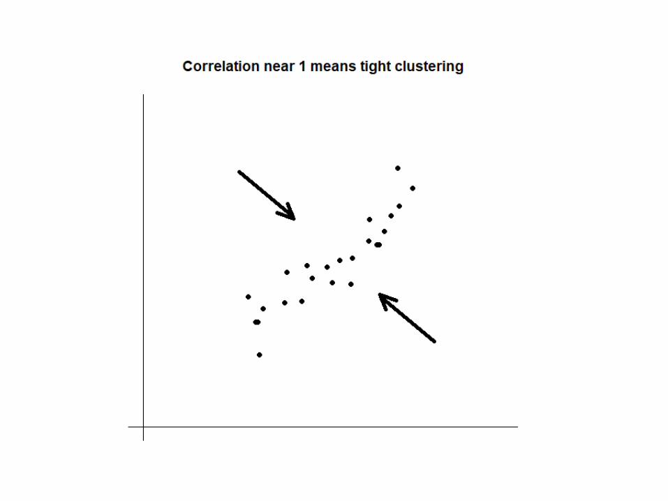
Let’s look at the following figures. In the first figure, the points in the cloud are tightly clustered around a line. Thus, there is a strong linear association between the two variables.

In the second figure, the points in the cloud are loosely clustered around a line. Thus, there is a not so strong linear association between the two variables.

The strength of the association in the two figures is different.

If the correlation coefficient is positive and close to one, then the two variables are directly related.

If the correlation coefficient is negative and close to minus one, then the variables are inversely related.

If the correlation coefficient is close to zero, then the two variables are not related (linearly).

EXAMPLE L8A: The figure below has six scatter diagrams for hypothetical data. The correlation coefficients, in scrambled order, are:

-0.99 -0.82 -0.15 0.01 0.65 0.99 Match the scatter diagrams with the correlation coefficients.

Computing r

After computing the averages and SDs, the correlation coefficient is computed as follows:

• Convert each variable to standard units.

• The average of the products is the correlation coefficient.

EXAMPLE L8B: For the data set (1,5), (1,3), (1,5), (1,7), (2,3), (2,3), (2,1), (3,1), (3,1), (4,1),

it can be shown that average of x-values = 2SD of x-values = 1average of y-values = 3SD of y-values = 2.Find the correlation coefficient for this data set.

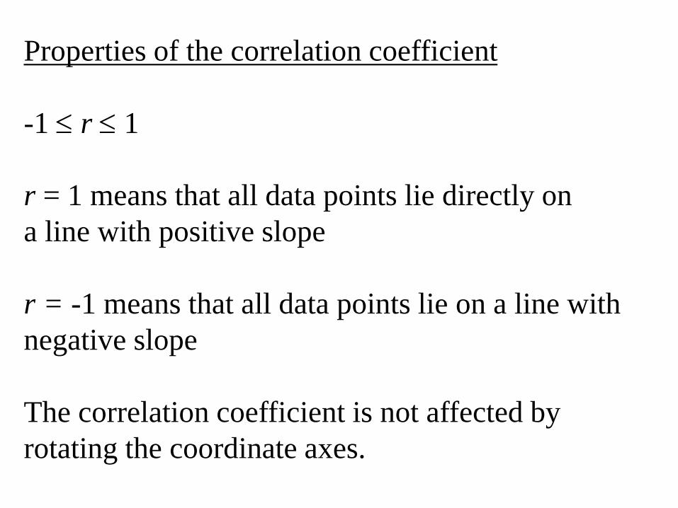
Properties of the correlation coefficient

-1 ≤ r ≤ 1

r = 1 means that all data points lie directly on a line with positive slope

r = -1 means that all data points lie on a line with negative slope

The correlation coefficient is not affected by rotating the coordinate axes.

EXAMPLE L8C: For the data set (1,1), (1,1), (1,1), (1,1), (2,3), (2,3), (2,3), (3,5), (3,5), (4,7),

it can be shown that average of x-values = 2SD of x-values = 1average of y-values = 3SD of y-values = 2.Find the correlation coefficient for this data set.

EXAMPLE L8D: Suppose we have a data set such that there are at least two distinct points and r is the correlation between x and y. True or false:

(a) If r = 1, then all of the points must lie on the same line.

(b) If all of the points lie on a line, then r = 1.

(c) If all of the points lie on a line, then r = 1 or r = -1.

(d) If r = 0, then all of the points must lie on a horizontal line.

(e) The correlation coefficient r cannot be greater than 1.

(f) The correlation coefficient must be greater than –1.

(g) If r = 0.8, then 80% of the points are clustered around a line.

(h) If r = 0.8 for one data set and is 0.4 for another data set, then the relationship between the two variables in the first set is twice as linear as the relationship in the second data set.

(i) If a data set is clustered around a line with a steeper slope than another data set, then it has a stronger correlation than that data set.

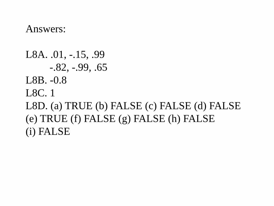
Answers:

L8A. .01, -.15, .99-.82, -.99, .65

L8B. -0.8L8C. 1L8D. (a) TRUE (b) FALSE (c) FALSE (d) FALSE (e) TRUE (f) FALSE (g) FALSE (h) FALSE (i) FALSE

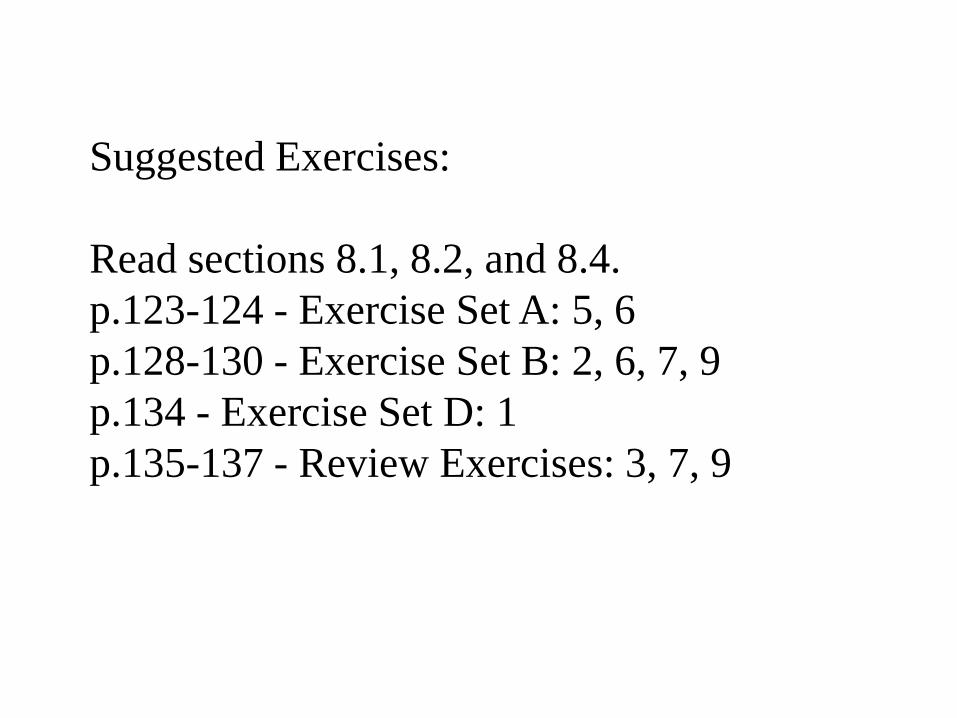
Suggested Exercises:

Read sections 8.1, 8.2, and 8.4.p.123-124 - Exercise Set A: 5, 6p.128-130 - Exercise Set B: 2, 6, 7, 9p.134 - Exercise Set D: 1p.135-137 - Review Exercises: 3, 7, 9