Remote Sensing GEOG 883: Spring 2010 Capstone Project

Page | 1

CLANDESTINE AIRSTRIPS: OPPORTUNITY FOR NARCOTICS-

TERRORISM NEXUS IN LAGUNA DEL TIGRE NATIONAL PARK,

GUATEMALA

Gerby Marks

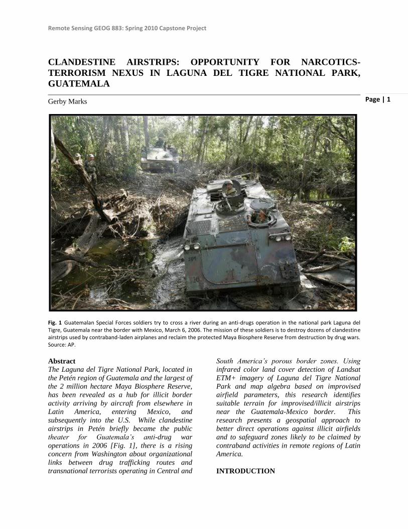
Fig. 1 Guatemalan Special Forces soldiers try to cross a river during an anti-drugs operation in the national park Laguna del Tigre, Guatemala near the border with Mexico, March 6, 2006. The mission of these soldiers is to destroy dozens of clandestine airstrips used by contraband-laden airplanes and reclaim the protected Maya Biosphere Reserve from destruction by drug wars. Source: AP.

Abstract

The Laguna del Tigre National Park, located in

the Petén region of Guatemala and the largest of

the 2 million hectare Maya Biosphere Reserve,

has been revealed as a hub for illicit border

activity arriving by aircraft from elsewhere in

Latin America, entering Mexico, and

subsequently into the U.S. While clandestine

airstrips in Petén briefly became the public

theater for Guatemala’s anti-drug war

operations in 2006 [Fig. 1], there is a rising

concern from Washington about organizational

links between drug trafficking routes and

transnational terrorists operating in Central and

South America’s porous border zones. Using

infrared color land cover detection of Landsat

ETM+ imagery of Laguna del Tigre National

Park and map algebra based on improvised

airfield parameters, this research identifies

suitable terrain for improvised/illicit airstrips

near the Guatemala-Mexico border. This

research presents a geospatial approach to

better direct operations against illicit airfields

and to safeguard zones likely to be claimed by

contraband activities in remote regions of Latin

America.

INTRODUCTION

Page | 2

Major concern has been raised about the

cooperative relationship among narcotics

traffickers and transnational terrorist groups in

Latin America‟s permeable borders—from the

Iguazu triborder zone of Argentina, Paraguay

and Brazil, the Colombia-Venezuela border to

the Guatemala-Mexico border. While the U.S. is

working to secure its border with Mexico from

MS-13, Al-Qaeda and others, it is critical that

the U.S. provide intelligence support to the

transnational Inter-American Committee Against

Terrorism (CICTE) to combat Islamist terrorism

as well as Latin America‟s anti-drug war. Of

particular relevance to the geospatial intelligence

(GEOINT) tradecraft is identification of

clandestine airstrips for transit of weapons,

drugs, and individuals. This research is therefore

directed to detection of suitable sites for

clandestine airstrip operation along the

Guatemala-Mexico border by geospatial

analytical techniques. This border zone is

especially critical to U.S. interests: it is a sieve

for illicit air trafficking from elsewhere in Latin

America and subsequent filtering into the U.S.

by other routes [Fig. 2].

Fig. 2 Suspected drug trafficking flights documented in 2003. The Guatemala-Mexico border is a way station for illicit activity. Source: White House Office of National Drug Control Policy.

The Laguna del Tigre National Park, located in

the Petén region of Guatemala and the largest of

the Maya Biosphere Reserve (MBR), has been

identified as a hub for illicit border activity. The

existence and ongoing creation of clandestine

airstrips in Laguna del Tigre is cited by

international ecologists and military alike,

despite the 2006 attempt by Guatemalan Special

Forces to eradicate the problem. Continuing

deforestation, induced and sustained by human

activity, exacerbates the problem by providing

new territory to be surreptitiously converted

from national parkland to contraband no-man‟s

land. MBR park and government officials in

Guatemala note the challenge in identifying and

responding to the problem in this remote region.

This research presents a first step for the U.S. to

extend its scientific and environmental

diplomacy and national security efforts to

protect the MBR, locate contraband activities,

and preemptively seal the Mexico-Guatemala

border.

STUDY AREA

Laguna del Tigre National Park is one of five

national parks, four biological reserves

(biotopes), a multiple use zone and a buffer zone

in northern Guatemala. Together, these

comprise 2 million hectares of land known the

Maya Biosphere Reserve (MBR) and are part of

Central America‟s largest continuous tropical

moist forest. The MBR is located in the Petén

department of Guatemala [Fig. 3].

Fig. 3 Locational Image of Maya Biosphere Reserve in El Peten, Guatemala. Source: Parkswatch.org

Page | 3

Laguna del Tigre is in the municipality of San

Andrés, department of Petén. The park is

bordered to the north, east and west and south by

the MBR Multiple Use Zone. The eastern and

northern borders lie just a few kilometers from

the edge of the Mexican states of Campeche and

Tabasco. Laguna del Tigre, including both

Laguna del Tigre-Park and Laguna del Tigre-

Rio Escondido which is nestled within the larger

park, covers 289,912 hectares, and is the largest

in Guatemala. The legally established borders lie

within 17° 11‟ 41” and 17° 48‟ 53.2” latitude,

and 90° 58‟ 2.8” and 90° 2‟ 44.2” longitude.

Land cover in Laguna del Tigre includes

transitional woodlands, oak forest, flooded

savannah, and marshes. For the purposes of this

study and to facilitate monitoring of Laguna del

Tigre and its immediate periphery, the region of

analysis selected includes both Laguna del

Tigre-Rio Escondido (which is circumscribed

within the National Park), Laguna del Tigre-

National Park as well as the Multiple Use slivers

which are monitored by Laguna del Tigre

officials as well as shown in the graphic below.

METHODS OVERVIEW

Vector and raster data and analytical outputs

selected for this project intend to evaluate the

Laguna del Tigre Park for suitable terrain for

extant and future improvised/illicit airstrips.

Data includes vector files provided by

Guatemala‟s Consejo Nacional de Areas

Protegidas (CONAP), Landsat TM 15 m

imagery from the 2005 Global Land Survey

(GLS) and 3” Shuttle Radar Topography

Mission (SRTM) Digital Elevation Model

(DEM).While the MBR spans UTM 15 and

16N, Laguna del Tigre is located in 15N and

data was thus projected to this zone. An

overview of the workflow is shown in Fig. 5. It

first identifies extant clearings based on 15 m

resolution satellite imagery, likely induced or

sustained by human intervention. Using 3”

DEM, terrain is then evaluated according to

airfield parameters of slope. ArcGIS and ENVI

will be used.

Remote Sensing GEOG 883: Spring 2010 Capstone Project

Page | 4

Fig. 5 Workflow Diagram.

ANALYTICAL WORKLFOW

DATA PREPARATION First, a new vector file for the Laguna del Tigre

complex was created, comprising both the Rio

Escondido, National Park, and Multi-Use Zones.

Composite band layers were stacked for the GLS

2005 Landsat TM, re-sorted into a 4,3,2

combination and then clipped to the Laguna del

Tigre region of analysis mask. The Landsat TM

band combination 4,3,2, or infrared color, was

selected rather than natural color to better

display wetlands and vegetation [Fig. 6]. As the

infrared version shows, actively growing canopy

appears bright red, bare soil appears blue-green,

and water appears black in this combination of

near infrared, visible red, and visible green

bands.

Fig. 6 A zone of Laguna del Tigre displayed in the “natural color” Landsat band combination 3, 2, 1 (top) and in the “infrared color” Landsat band combination 4, 3, 2 (bottom).

AIRSTRIP SUITABILITY

IDENTIFICATION

SLOPE SUITABILITY

CLANDESTINE

AIRFIELD

PROBABILITY

Use ENVI to load GeoTiff MTL file and stack layers for export to ArcGIS, display Landsat with 4, 3, 2 band image.

Use unsupervised classification to create and identify land cover types.

Rename and reclassify land cover types based on airfield suitability parameters of non- moist soil and cleared land.

Calculate slope for DEMs and use map algebra to locate all pixels with slope <2%.

Assign all slope with <2% a value of 1 and >2% a value of 999.

Identify highly ranked clusters (lowest values) that meet the suggested minimum length and width for a personal airstrip (75 feet wide in open grassy areas, 200 feet wide in wooded areas, 3200 feet in length).

SLOPE & LAND COVER

CALCULATION

CLANDESTINE

AIRFIELD

PROBABILITY

Use map algebra to calculate all pixels in terms of slope classification values and with land cover classification values.

LAND COVER DETECTION &

CLASSIFICATION

Page | 5

LAND COVER DETECTION &

CLASSIFICATION

Pixels from the infrared color GLS 2005 were

next sorted into different land cover types. Both

supervised and unsupervised classes as well as

different n classes and training sets were tested.

Without having ground-test data, visual

examination showed that unsupervised

classification and 8 classes performed the best

for distinguishing between land cover types in

Laguna del Tigre for the purposes of this

investigation [See Fig. 7]. In addition, the 4,3,2

combination helped detect and classify areas that

might be “clear” of canopy but are in fact soggy

zones, including marshes and flooded savannah.

The ability to simultaneously detect ground

moisture with land cover proved significant

because digital soil data available for Guatemala

is at too coarse a resolution to bring additional

insight into this study. The eight classes were

defined as water/flooded savannah, marshes,

dense forest canopy, transitional forest, light

vegetation, transitional clearing, light clearing,

and full clearing.

Fig. 7 Unsupervised Classification with 8 classes proved to be the best method for detecting and defining land cover classes in Laguna del Tigre.

Fig. 8 Graph of quantified Land Cover classes in Laguna del Tigre.

These land cover types are represented as shown

in Fig. 8 within Laguna del Tigre. Water/

flooded savannahs, marshes, dense canopy,

transitional forest comprise an increasingly

smaller amount of coverage each year in Laguna

owing to human intervention (For comparison

see GLS 2000 of the same region). It is not

surprising to see that land cover ripe for human

activity comprises 46.2% of Laguna del Tigre.

The land cover types were next reclassified

according to their suitability for building illicit

airstrips as Fig. 9 shows. Rankings 1-5

represents the most to least likely to have extant

airstrips, owing the existence (and perhaps

human maintenance) of cleared terrain. Light

vegetation is ranked 15 because this area, while

occupied by woody shrub, is not particularly

dense or difficult to remove. Indeed, the ever

shrinking forest of the MBR suggests that in

2010, light vegetation areas may now be cleared.

Transitional forest, dense forest canopy,

LAND COVER IN LAGUNA DEL TIGRE Class Percent Coverage of Total Analysis Area

and Pixel Count

Unsupervised classification, 8 classes

17.1 %

16.5 % 15.3%

14.1%

12.9%

7.5% 12.8% 3.8%

Page | 6

marshes, water and flooded savannah have all

been assigned 999 as “impossible” values. While

an airstrip may be built within a vegetative

copse, it is probable that the bare soil or cleared

ground would be visible from the satellite

image.

Fig. 9 Table of Land Cover Types and reclassified values.

SLOPE SUITABILITY

The next phase of analysis considered the basic

parameter of slope necessary to create an

improvised airstrip. A raster slope map was

created from the 3” DEM SRTM. Terrain with

slope < 2% was identified as for airstrip or not

possible and pixels were classified with values

of 1 (Y) and 999 (N) as shown in Fig. 10.

Fig. 10 Reclassified slope values in the Maya Biosphere Reserve.

Fig. 11 Output of Slope & Land Cover Calculation for Laguna del Tigre.

SLOPE & LAND COVER CALCULATION

The reclassified values of both slope and land

cover were multiplied to identify pixels with

both slope < 2% and appropriate land

cover/ground moisture for building an

improvised airstrip. Pixels values 1, 5, and 15

from the map algebra were retained for further

analysis [Fig. 11], with 1 as the highest rank

(slope <2% and light or full clearing) and 15

(slope < 2% and light vegetation) as the lower

rank for airstrip probability. However, owing to

stringent parameters for values assigned to land

cover, all ranks 1 through 15 represent very real

possibility of extant or future airstrips.

IDENTIFY AIRSTRIP OPPORTUNITY

The last phase of analysis involved visual

scanning of pixel clusters ranked 1-15 to identify

clusters that provided enough area to locate the

minimum suggested requirements for an airstrip

in open and wooded terrain. These parameters

are: a minimum of 3200 ft (975.36 m) in length,

75 ft (22.86m) width in open, grassy terrain or

200 ft (60.96m) width in wooded terrain.

Airstrip lines were digitized at the minimum

Land Cover Value

water/flooded savannah 999

marshes 999

dense forest canopy 999

transitional forest 999

light vegetation 15

transitional clearing 5

light clearing 1

full clearing 1

Page | 7

suggested length and with width buffers set to

11.5 m on each side and 30.5 m on each side to

account for possible variation in minimum

width. While not every single airstrip

opportunity was identified, “hotspots”, or terrain

with multiple opportunities for airstrips, were. It

should be noted that opportune pixel clusters

were interrupted by intermittent “impossible”

pixels. For the most accurate assessment of

airstrip opportunity, it would be important to

double check these “impossible” pixels and to

potentially recalculate the data. This might

include allowing for a slightly larger slope (i.e.

2.5%) or to check the “impossible” pixel against

the original Landsat 4, 3, 2 imagery to verify

that the pixel was appropriately classified with

respect to land cover. The identification of

broader “hotspots” and actual geographic

locations of specific airstrips intends to provide

a simple compensation for the aforementioned

uncertainty in the final classification. Figures 12

and 13 demonstrate the final outputs.

Fig. 12 (above) and 13 (below) Digitized potential airfield locations, based on presence of pixel clusters valued 1-15. Airfields are shown with the minimum requirements for open, grassy terrain and with a width buffer for wooded terrain. There is clearly ample for room for all manner of illicit airstrip in the detail image in the lower left. Such zones have been identified as “hotspots” with digitized polygons.

Page | 8

Fig. 13 The upper image shows the possibility of digitizing unimproved roads, visible in the infrared color satellite image, and linking these to airstrip hotspots. This spectral cluster on the periphery of Laguna del Tigre is prime for security investigation.

Page | 9

CAVEATS The short timeframe of this capstone project and

especially the limitation to public geospatial data

confines the ability for this analysis to meet high

standards of accuracy or timeliness for

Guatemalan Special Forces. Analysis and

tactical planning could be significantly improved

with more current imagery as well as digitization

of park infrastructure, as rudimentary as it may

be. There is much licit activity in Laguna del

Tigre in recent years that remains to be tracked

and mapped: recent investigations at sites of

archaeological significance (El Peru) as well as

biological research facilities (Guacamayas

Biological Station) and tourist hostels (if any).

In geospatially analyzing terrain of a largely

(digitally) unmapped region, it is critical to

identify legal and beneficial land usage to ensure

there is no conflict of analysis.

FINDINGS & CONCLUSION

Although these findings are based solely on

satellite imagery collected in 2005, they

nonetheless suggest a reasonable method to

objectively identify, prioritize, and—with the

inclusion of digitized Laguna del Tigre trail

maps—coordinate on-the-ground operations by

Guatemalan Special Forces and/or to create a

monitoring route for CONAP and conservation

officials. Additionally, creation of a geographic

visualization for securing Laguna del Tigre

provides Guatemalan, Mexican, and U.S. forces

alike with a common operational picture. While

Guatemala security undertook an anti-

contraband mission to Laguna del Tigre in

March 2006, it is unknown how many

clandestine airstrips were discovered and

destroyed or what hearsay information the

operations were based upon, let alone what

potential zones remain unchecked. Indeed, with

continuing deforestation in Laguna del Tigre,

opportunities for contraband activities along its

remote periphery have certainly increased since

the imagery used for this analysis, acquired in

2005. Moreover, U.S. concerns for the

narcotics-terrorism nexus operating in

coordinated trafficking routes across Latin

America, and for ultimate destination into the

United States, makes the Guatemala-Mexico

border a region of heightened and immediate

concern. The Maya Biosphere Reserve, a

protected, biodiverse landscape with significant

archaeological remnants and species of flora and

fauna demands special treatment in the fight

against drugs, weapons, illicit migration, and

organized crime training/trafficking. Geospatial

analysis for detection of illicit activity in

deforested terrain provides a non-invasive

approach for international authorities to identify

and intervene, or to provide Guatemalan

officials with the necessary information to

protect the borders of the Americas, her

landscape, people and heritage.

Overall, this research suggests that the GEOINT

tradecraft has tremendous opportunity to address

and confront the most elusive, illicit activities in

the most remote regions of the world.

REFERENCES

(2009). “Terrorism and Drug Routes.” Center

for Threats Awareness. March 27 2009.

http://threatswatch.org/rapidrecon/2009/

03/terrorism-and-drug-routes/

(2009). “Hezbollah uses Mexican Drug Routes

in to the U.S.” The Washington Times.

March 27 2009.

http://www.washingtontimes.com/news/

2009/mar/27/hezbollah-uses-mexican-

drug-routes-into-us/

(2009). “Border Lawmakers Fear Drug-

Terrorism Link.” March 7, 2009.

http://www.house.gov/list/hearing/az02_

franks/thehill_franks_border_Mar72009.

html

(2008). “Fears of a Hezbollah Presence in

Venezuela.” The Los Angeles Times.

August 27.

http://articles.latimes.com/2008/aug/27/

world/fg-venezterror27

(2008). “Guatemala boosts armed presence on

border with Mexico.” The Los Angeles

Times. September 27.

Page | 10

http://latimesblogs.latimes.com/laplaza/

2008/09/guatemala-ups-a.html

Chepesiuk, Ron. (2007). “Dangerous Alliance:

Terrorism and Organized Crime.”

September 11. Global Politician.

http://www.globalpolitician.com/23435-

crime

Choi, Charles Q. (2008). “Drug traffickers and

other outlaws endanger forest

preservation efforts.” Scientific

American Magazine. October.

http://www.scientificamerican.com/artic

le.cfm?id=drug-traffickers-endanger-

preservation

Ciment, James D. and Frank G. Shanty (2008),

eds. Organized Crime: From

Trafficking to Terrorism, Vol. 1. Santa

Barbara: ABC-CLIO.

Craddock, Gen. Bantz J. (2006) “The Americas

in the 21st Century: The Challenge of

Governance and Security”.

FIU/AWC/SOUTHCOM Conference.

February 2.

http://www.southcom.mil/AppsSC/files/

1UI1I1169398593.pdf

Craddock, John and Barbara Fick. “The

Americas in the 21st Century: The

Challenge of Governance and Security.”

http://www.dtic.mil/doctrine/jel/jfq_pub

s/4208.pdf

Forero, Juan. (2008). “Venezuela steps up

efforts to thwart cocaine traffic.” The

Washington Post. April 17.

http://www.washingtonpost.com/wp-

dyn/content/article/2008/04/06/AR2008

040602158.html

Gato, Pablo and Robert Windrem. “Hezbollah

Builds a Western Base.”

http://www.hacer.org/current/LATAM2

28.php

Grainger, Sarah (2008). “Budget Woes Weaken

Guatemalan Army.” Reuters. October 2.

www.reuters.com/article/idUSN022631

40

Hudson, Rex (2003). Terrorist and Organized

Crime Groups in the Tri-Border Area of

South America. Federal Research

Division, Library of Congress.

http://www.loc.gov/rr/frd/pdf-

files/TerrOrgCrime_TBA.pdf

Sader, Steven and Daniel Hayes (2001).

“Comparison of Change-Detection

Techniques for Monitoring Tropical

Forest Clearing and Vegetation

Regrowth in a Time Series .”

Photogrammetric Engineering &

Remote Sensing. September 67(9):1067-

1075.

Sader, S.A. C. Reining, T. Sever, and C. Soza

(1997). “Human migration and

agricultural expansion: a threat to the

Maya tropical forests.” Journal of

Forestry 95: 27-32.

Sader, S.A., D.J. hayes, M. Coan and C. Soza

(2001). Forest change monitoring of a

remote biosphere reserve. International

Journal of Remote Sensing 22: 1937-

1950.

Schmid, Alex (2008). “Drug Trafficking,

transnational crime, and International

Terrorist Groups.” In Organized Crime:

From Trafficking to Terrorism, Vol. , ed.

by James D. Ciment and Frank G.

Shanty. 342-345.

http://www.wikihow.com/Build-a-Grass-

Landing-Strip

IMAGE SOURCES

Fig 1. www.militaryphotos.net/forums/showthread.php?77266-Today-s-Pic-s-Sunday-April-02-2006

Fig. 2 http://www.npr.org/news/images/2007/oct/12/suspect_tracks_map2006.jpg

Fig 3. http://www.parkswatch.org/parkprofiles/maps/ltre_eng.gif

Page | 11

APPENDIX I: DATA SPECIFICATION & SOURCES Raster Data

SRTM 1" DEM, 30 m resolution. 2002. srtm_18_09.img. Source: http://edcsns17.cr.usgs.gov/EarthExplorer/

2005 Global Land Survey Satellite Multispectral Image, 15 m

resolution. Landsat 7ETM+ and Landsat 5 TM (2003-2008) WRS-2, Path 020, Row 048,

Coordinates: 17°18'47.16"N, 90°14'33.36"W, Acquisition date 2005-04-10. Entity ID: LE70200482005100ASN00 Source: http://glcfapp.glcf.umd.edu:8080/esdi/index.jsp GEOTIFF

file.

2000 Global Land Survey Satellite Multispectral image, Pixels are subsampled to a resolution of

255 meters from the original 30-meter data, Landsat 7 ETM+ and Landsat 5 TM (1999 - 2003)

WRS-2, Path 020, Row 048, Coordinates: 17°20'53.85"N, 90°12'34.38"W, Acquisition Date:

2000-3-27. Entity ID: P020R047_7X20000327 Source:

http://glcfapp.glcf.umd.edu:8080/esdi/index.jsp TIFF files (no MTL file)

2010 MODIS AQUA Satellite [Base Map] 7, 2,1 Band Combination, 250 m resolution.

Acquisition date: 2010-01-07. Source: http://earthobservatory.nasa.gov TIFF file.

Vector Data

National Park Boundary files for the Maya Biosphere Reserve and Laguna del Tigre. Consejo

Nacional de Area Protegidas (CONAP) of Guatemala. Courteously provided by Fernando Castro,

Director of CONAP, 2010-03-18. fercastro@conap.gob.gt. ESRI shapefile format.

Political Boundary Files. Guatemala/Mexico border, boundaries for the Petén department and its

municipalities. www.gadm.org ESRI shapefile format.

Other country files www.gisdatadepot.org (Digital Chart of the World). ESRI Shapefile format

Page | 12

APPENDIX II: CLASSIFICATION & PROCESS

INTRODUCTION

The objectives of this project were twofold: first,

to see if geospatial analysis of remotely sensed

data in the Maya Biosphere Reserve (MBR)

could be useful in detecting opportunities for

illicit activities in remote regions of interest to

U.S. security, such as clandestine airstrips in

Laguna del Tigre National Park. This report

intended to be an initial attempt to prove the

process, methodology and applicability of

GEOINT tradecraft in assisting our anti-

narcotics and anti-terror allies in Latin America.

It accomplished this. However, this research

project also seeks accuracy, reliability, and

repeatability with regards to spectral

classification of land cover with satellite

imagery for the MBR. Indeed, the land

classification scheme must be carefully thought

out, experimented with and validated, if the

overall analysis is to prove useful and reliable.

Owing to constraints of time, familiarity with

software, and scope of work, the above research

based its analysis on unsupervised classification

of the GLS2005 imagery, accomplished through

ArcGIS. This appendix, however, describes the

experimentation and exploratory learning of the

researcher‟s classification technique with both

ENVI and ArcGIS software platforms for GLS

2000 and GLS 2005 data of the MBR. At the

end, ArcGIS unsupervised classification was

selected for the report because it appropriately

and objectively defined the terrain in terms of

classes that could prove meaningful in terms of

both ground cover and ground moisture. And, it

was important to identify a fairly reliable

classification scheme that the researcher felt

comfortable with rather than exhaust all the

possibilities, given the scope of the project.

This appendix intends to present the layer of

experience gained from exploring classification

processes for (or generation of land cover types

from) remotely sensed data. Generation of land

cover from remotely sensed imagery is essential

to the premise of this project, and ultimately,

most be “got right.” In the long term, I seek to

learn the most effective method of targeting

areas for clandestine airstrips and for similar

applications, such as training camps in remote

regions. The research experimentation herein

describes my first steps towards gaining more

familiarity with ENVI and ArcGIS tools for

classification.

First, a note about the remotely sensed imagery

itself. The initial intent of this project was to

locate the most current data available and to

detect land change over time as a first step in the

process. However, after learning that Landsat 7

+ETM scan line corrector went out in 2003 (and

the images I intended to use were indeed striped

and incomplete), I used the Landsat

7+ETM/Landsat 5TM Global Land Survey

(GLS) 2005 for my analysis. This was the best

quality and most recent image I could track

down publicly of the study area. In addition, the

Global Land Survey 2000 provided an excellent

multispectral view of the region. The GLS 2000

was in fact noted by NASA and observed by the

researcher as being a much superior quality

image and of possible use in future stages of

analysis (Global Land Survey 2000 could

provide the „before theme‟). The GLS 2005 had

a striping pattern that may have interfered with

appropriate classification as shown in Fig. 1,

while the GLS 2000 was much crisper in detail

(although at a lower resolution) and lacked these

patterned blurs across the image. Out of interest

in gaining familiarity with the region and

different image qualities, I experimented with

GLS 2000 in ENVI and GLS 2005 in ArcGIS

and opted to use the GLS2005 in my project

since this was the most recent imagery and I did

not feel that the patterned blur impacted the

landcover type output in either the classified or

unclassified processes I worked with.

Fig. 1 Striping visible in GLS 2005. Will this significantly impact my classification of land cover types?

ArcGIS CLASSIFICATIONS

In ArcGIS I tested both supervised and

unsupervised classification of GLS 2005.

UNSUPERVISED

For unsupervised classification, a range

of classes were tried, to determine the best fit to

the land cover types. Starting at 5 and working

to 10, it was determined that 5 classes were too

little (water was not being distinguished) and 10

offered too much differentiation for the purposes

of this research. The number eight was selected

and the land cover types identified and classed

essentially matched the 9 I describe below and

which I selected for the representative types for supervised classification. Water/flooded

savannah were combined in this case (in the

supervised training set, I distinguished between

them) since the unsupervised set of 8 seemed to

combine them and the 9 unsupervised

classification seemed off. This worked fine for

my analysis since both water and flooded

savannah would be labeled as “impossible” or

given a pixel value of 999 for the map algebra

component. Also, since my analysis ended up

not comparing images, looking for change

detection over time, it was possible to use

unsupervised classification.

SUPERVISED: Development of

Classification Training Set

After consulting various articles on

Laguna del Tigre‟s land cover and comparing it

to my research needs and to the Central

American Vegetation Classification scheme, the

next step was to select a representative,

paradigm case of each land cover types and train

the computer to label all similarly occurring

pixels as the same. The land cover types I

selected were water, flooded savannahs,

wetlands, dense oak forest canopy, transitional

forest, light vegetation, transitional clearing,

light clearing, and clearing. These representative

areas were constructed as a Training Set vector

layer in ArcGIS. Nine polygons with five

sample of each representation were constructed

as representation of the range of landcover type.

These vectors could then be loaded over the

georeferenced Landsat image in ArcGIS. I

sampled image using the training set with the

four classification techniques available in

ArcGIS:

Parallelepiped Classification based on a decision rule based on the standard deviation from the mean of each defined and trained class.

Maximum Likelihood Assumes normally distributed statistics for each class and uses the probability of each pixel belonging to each class.

Mahalanobis Distance Direction sensitive variant of the Maximum Likelihood scheme that takes into account the spatial distribution of surrounding, similar pixels.

Minimum Distance Calculates the Euclidean distance between the defined class vector and the vector describing the pixel to be classified to determine which class a pixel belongs to.

Fig. 1 Summary of Supervised Classification Processes available in ArcGIS

.Assessment and Selection of Classification

Schemes

Image results are shown below. As ground truth

data could not be used to test the reliability of

the different classification schemes, the task of

evaluating the effectiveness of the

classification methods was carried out with

the help of the same GLS 2005 image. By

visually inspecting the fit of class polygons

around vegetative features in the satellite

photos, it could be estimated which

technique was most effective at identifying

the nine land cover types. Immediately it

was apparent that the parallelepiped method

grossly over-estimated the extent of. The

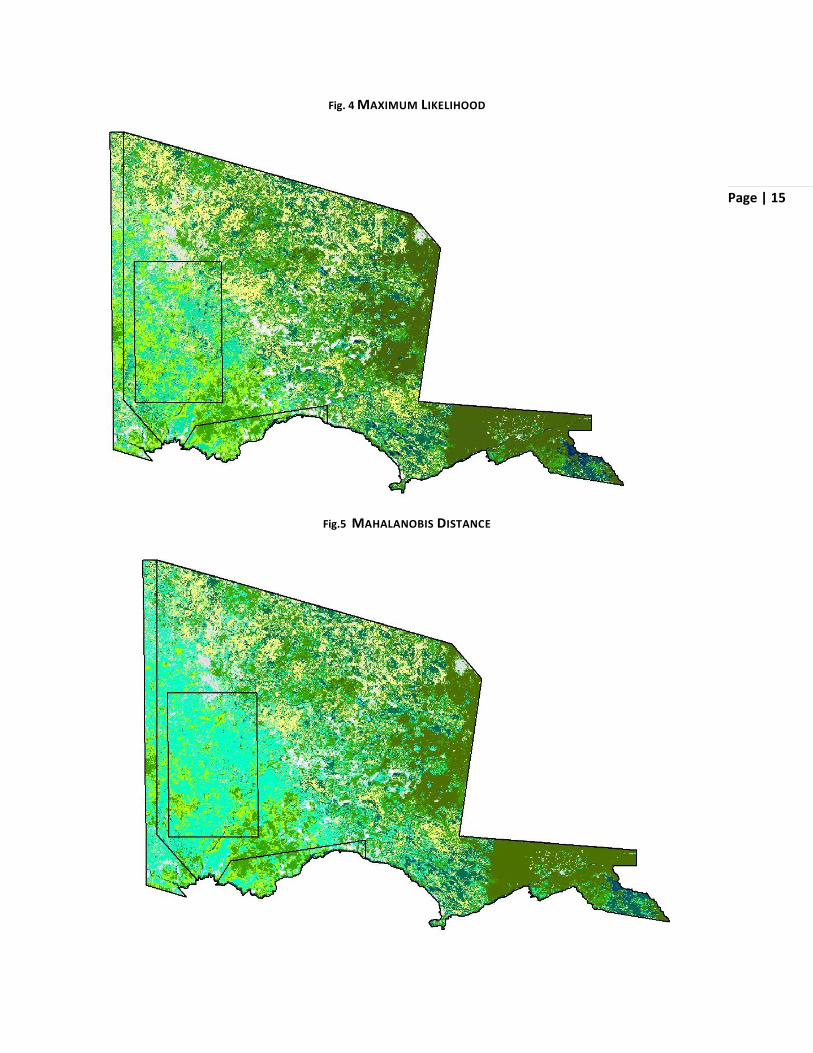
mahalanobis distance technique tended to

over-estimate the extent of marsh cover and

showed a large amount of "blotting" in the

densely forested areas. The parallelpiping

method seems to overestimate medium

clearings and underestimate marshes,

flooded savannah and water. The minimum

distance accounted for the variation in the

landcover, bringing more “light canopy”

blots into “clear regions” and “clear regions”

into “transitional forest,” however it seemed

to over-estimate the extent of water, bring

more blotting into what I observed to be

flooded savannah and marsh land covers.

Maximum likelihood provided a slightly

better fit in terms of water (what was water

in the minimum likehilhood often became

flooded wetlands), but lacked the

complexity of variation that I observed in

the image and that the minimum likelihood

algorithm offered. Again, since all water and

moist open terrain are unsuitable in the

subsequent map algebra, I decided that the

minimum likelihood algorithm produced, by

far, the best representation of clearings in

the Laguna del Tigre region of analysis in

the MBR. Owing to time constraints, I did

not repeat the full process of analysis for

airfield suitability using these

classifications. However, it would have

been very interesting to compare the output

of this method with that of the untrained

classification which I ultimately used.

Land Cover Type Training Set for All Classifications

Fig. 3 PARALLELPIPED

Page | 15

Fig. 4 MAXIMUM LIKELIHOOD

Fig.5 MAHALANOBIS DISTANCE

Page | 16

Fig.6 MINIMUM DISTANCE

ENVI CLASSIFICATIONS

In ENVI both supervised and

unsupervised methods were tested. First, the

data required pre-processing the individual band

files for the GLS 2000 image into layer stacks. I

could then proceed with analysis. The ENVI

manual proved essential in describing to me the

multiple ways to classify and to tweak

classifications. For this project, I intended to

develop a baseline understanding of the different

processes, how they differed from ArcGIS and

to test out a few that I had not used with ArcGIS

to see if I found them to be any better of a fit for

the data.

UNSUPERVISED

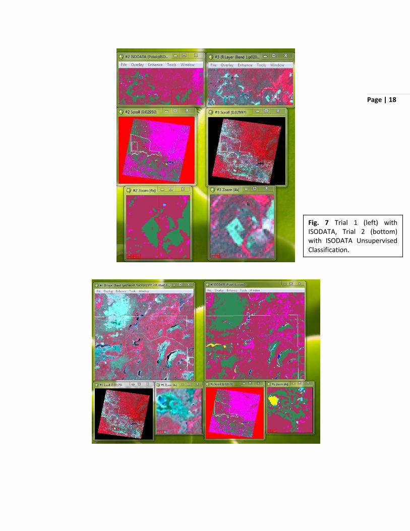
I tested out unsupervised ISODATA

classification which calculates class means

evenly distributed in the data space then

iteratively clusters remaining pixels using

minimum distance techniques. Iterations involve

recalculation of means, reclassification of pixels,

and class splitting, merging, and deleting is

accomplished based on input threshold

parameters. The process continues until the

maximum number of iterations is reached. This

process is certainly a step above ArcGIS in

terms of explaining the “magic” behind

unsupervised classification and permitting the

researcher to change the ISODATA parameters.

For my first try, I selected only one iteration, 1

pixel per class, and a range of 5 to 10 for classes.

The second time I used two iterations, 4 pixels

per class, and a range of 7 to 9 classes. Screen

Captures of Trial 1 (top) and Trial 2 (bottom) are

included below.

SUPERVISED: Classification Training Set

I focused primary on Spectral Angle

Mapper to see if I could translate what we

learned in Lesson 7 to my investigation. Since I

didn‟t have an extant spectral library file to work

from, I collected endmember spectra from the

plot window. The experience of selecting a

Page | 17

single pixel to define an endmember group

seemed challenging and too precise for me to

account for the wide variety of classes and pixel

colors. This, however is where the option to

adjust the angle for each pixel comes in! and to

evaluate and revaluate whether you have the

right number of classes to identify all the cover

types. For this test I identified 7 classes, and a

pixel for each. I used the .10 radian as a single

value and chose no rule. The results are featured

below. This certainly should have been tried

with various configurations (9 classes, angle

variation).

Page | 18

Fig. 7 Trial 1 (left) with ISODATA, Trial 2 (bottom) with ISODATA Unsupervised Classification.

Page | 19

Fig. 8 Spectral Angle Mapper output using spectral library created from the original image, with seven classes.

REVIEW & FINDINGS

Software Assets

In terms of sheer maneuverability of

multiple windows at different scales, and the

ability to link displays, ENVI provides superb

opportunity to visually check the fit of different

classification strategies against the original

satellite image (See image below). The

exportability to ArcGIS and opportunity to bring

vector files into ENVI is fantastic, since I think

ENVI is overall a much superior tool for spectral

classification but not so user friendly in terms of

other components and toolbars in ArcGIS. My

primary concern is with the amount of time it

took me to work with the ENVI files properly

(on occasion I had difficulty getting the Z profile

spectrum to load, especially for the MTL of the

GLS2005, and there were several times that the

IDL stopped working/crashed). For GEOINT

applications, given the number of options ENVI

offers for classification seems daunting. In a

field where timeliness is key, ArcGIS seems to

provide simple and usable methods. However, I

believe that once I gain more familiarity with

ENVI and its own quirks for handling data, the

speed with which I could test out different

classification techniques with ENVI will surely

increase. I realize the software‟s exceptional

power to manage multi and hyperspectral

images and classification. For in-depth

environmental research, ENVI would be

indispensable.

As a software platform, I am much more

familiar with ArcGIS and it took much less time

to accomplish what I wanted. I also felt very

comfortable with the selection of polygons

rather than individual pixels to represent

different land cover types, as I felt that a range

of pixels was necessary to describe land cover in

the case of the MBR GLS images. At the same

time, the classification processes accomplished

by ArcGIS are far more automated than they are

in ENVI. No options are provided such as

setting threshold options and the mathematical

work behind the classification is “invisible” to

the researcher. I think it is important to

understand how and why the classification

systems work, by actively being able to alter

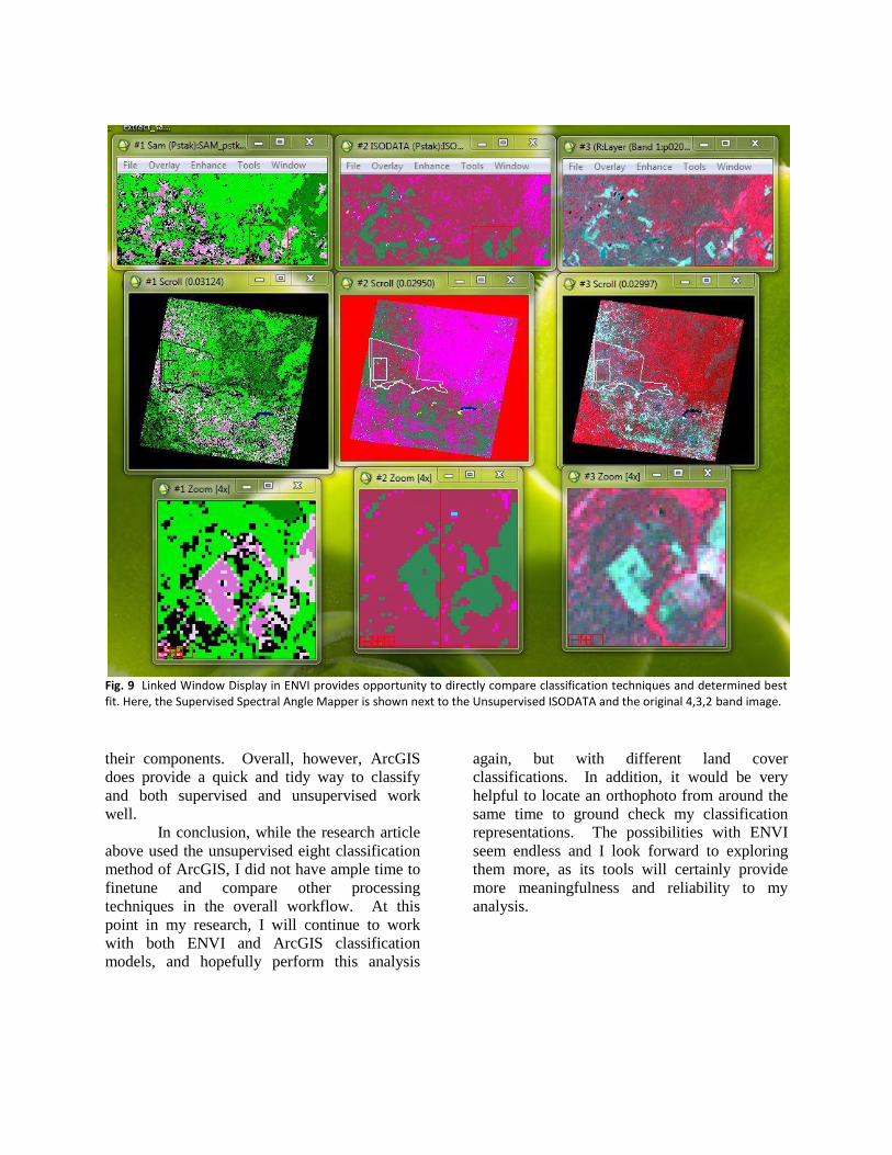
Fig. 9 Linked Window Display in ENVI provides opportunity to directly compare classification techniques and determined best fit. Here, the Supervised Spectral Angle Mapper is shown next to the Unsupervised ISODATA and the original 4,3,2 band image.

their components. Overall, however, ArcGIS

does provide a quick and tidy way to classify

and both supervised and unsupervised work

well.

In conclusion, while the research article

above used the unsupervised eight classification

method of ArcGIS, I did not have ample time to

finetune and compare other processing

techniques in the overall workflow. At this

point in my research, I will continue to work

with both ENVI and ArcGIS classification

models, and hopefully perform this analysis

again, but with different land cover

classifications. In addition, it would be very

helpful to locate an orthophoto from around the

same time to ground check my classification

representations. The possibilities with ENVI

seem endless and I look forward to exploring

them more, as its tools will certainly provide

more meaningfulness and reliability to my

analysis.