complex analysis mario bonk - uclambonk/246c.1.12s/complana.pdf · complex analysis mario bonk...
TRANSCRIPT
Complex Analysis
Mario Bonk
Course notes for Math 246A and 246B
University of California, Los Angeles
Fall 2011 and Winter 2012


Contents
Preface 6
1 Algebraic properties of complex numbers 8
2 Topological properties of C 18
3 Differentiation 26
4 Path integrals 38
5 Power series 43
6 Local Cauchy theorems 55
7 Power series representations 62
8 Zeros of holomorphic functions 68
9 The Open Mapping Theorem 74
10 Elementary functions 79
11 The Riemann sphere 86
12 Mobius transformations 92
13 Schwarz’s Lemma 105
14 Winding numbers 113
15 Global Cauchy theorems 122
16 Isolated singularities 129
17 The Residue Theorem 142
18 Normal families 152
19 The Riemann Mapping Theorem 161
3
CONTENTS 4
20 The Cauchy transform 170
21 Runge’s Approximation Theorem 179
References 187


Preface
These notes cover the material of a course on complex analysis that I taughtin the fall quarter of 2011 and the winter quarter of 2012. In many respects Iclosely follow Rudin’s book on “Real and Complex Analysis”. Since WalterRudin is the unsurpassed master of mathematical exposition for whom I havegreat admiration, I saw no point in trying to improve on his presentation ofsubjects that are relevant for the course.
The notes give a fairly accurate account of the material covered in class.They are rather terse as oral discussions that gave further explanations orput results into perspective are mostly omitted. In addition, all pictures anddiagrams are currently missing as it is much easier to produce them on theblackboard than to put them into print.
6

1 Algebraic properties of complex numbers
1.1. Intuitive idea. Complex numbers are expressions of the form a + biwith real numbers a and b. Here i is the imaginary unit. One computes (i.e.,adds and multiplies) with complex numbers as usual, but sets i2 = i ·i := −1.For example,
(3 + 5i)(2 + i) = 6 + 10i+ 3i+ 5i2 = 6 + 13i− 5 = 1 + 13i.
1.2. Definition of the complex numbers. For a rigorous definition welet the set of complex numbers be
C := (a, b) : a, b ∈ R
with the correspondence (a, b) ∼= a+ bi in mind. Addition and multiplicationare defined accordingly:
(a, b) + (c, d) := (a+ c, b+ d),
(a, b) · (c, d) := (ac− bd, ad+ bc).
One often omits the multiplication sign and writes zw := z · w for z, w ∈C. One also uses the convention that multiplication binds stronger thanaddition. So u+ vw = u+ (v · w) for u, v, w ∈ C, etc.
That one computes with complex numbers “as usual” is mathematicallyexpressed by the following fact.
Theorem 1.3. (C,+, ·) is a field, that is:
1. (C,+) is an abelian group, which means that
1.1 the addition + is associative,
1.2 there exists a neutral element 0 := (0, 0) ∈ C with respect toaddition,
1.3 every element (a, b) ∈ C has an (additive) inverse (−a,−b) ∈ C,
1.4 the addition + is commutative.
2. (C,+, ·) is a commutative ring, which means that
8
1 ALGEBRAIC PROPERTIES OF COMPLEX NUMBERS 9
2.1 (C,+) is an abelian group,
2.2 the multiplication · is associative and commutative,
2.3 the distributive law holds.
3. (C∗, ·) is a group, where C∗ := C \ 0.The proof is straightforward, but tedious, and so we skip it.
Remark 1.4. If we write (for the moment), a := (a, 0) ∈ C for a ∈ R, then
a+ b = (a, 0) + (b, 0)
= (a+ b, 0) = a+ b,
and
a · b = (a, 0) · (b, 0)
= (ab, 0) = ab.
This means that with expressions a, b, etc., one can compute in exactly thesame way as with the underlying real numbers a, b, etc. More precisely, themap
ϕ : R→ C, a ∈ R 7→ ϕ(a) := a,
is a field isomorphism of R onto its image in C.Accordingly, one “identifies” the image of R under ϕ with R, writes a
instead of a, and considers R as subset of C.Now let i := (0, 1). Then for a, b ∈ R we have
(a, b) = (a, 0) + (0, b)
= (a, 0) + (b, 0) · (0, 1)
= a+ bi = a+ bi.
So every complex number z ∈ C can uniquely be written as z = a+bi, wherea, b ∈ R. Note also that we have
i2 := i · i = (0, 1) · (0, 1)
= (−1, 0)
= −1 = −1.
Using these conventions we reconcile the precise definition of complex num-bers and their operations with the intuitive notion that we took as out start-ing point.

1 ALGEBRAIC PROPERTIES OF COMPLEX NUMBERS 10
Definition 1.5. Let z = a+ bi ∈ C, where a, b ∈ R. We define
(i) Re(z) := a (the real part of z),
(ii) Im(z) := b (the imaginary part of z),
(iii) z := a− bi (the complex conjugate of z),
(iv) |z| :=√a2 + b2 (the absolute value of z).
1.6. Geometric interpretations. These concepts and also addition ofcomplex numbers have obvious geometric interpretations if one identifies z =a+ bi with the point (a, b) in the plane R2.
1.7. Subtraction and division. As in every field one can define a notion ofsubtraction and division of complex numbers. Namely, if z ∈ C, one denotesthe additive inverse of z by −z and defines
w − z := w + (−z)
for z, w ∈ C. If z = a+ bi, w = c+ di, then −z = (−a) + (−b)i, and so
w − z = (c− a) + (d− b)i.
If z 6= 0, then we denote by z−1 the (multiplicative) inverse of z. For z =a+ bi 6= 0 we have
z−1 =a
a2 + b2− b
a2 + b2i.
One definesz/w =
z
w:= w · z−1.
One can compute with fractions of complex numbers as usual (as in any field).Using the fact that zz = |z|2, one can simplify fractions of complex numbersby multiplying in numerator and denominator by the complex conjugate ofthe denominator. For example,
2 + i
3 + 5i=
(2 + i)(3− 5i)
(3 + 5i)(3− 5i)
=(6 + 5) + (−10 + 3)i
32 + 52
=11− 7i
34=
11
34− 7
34i.
1 ALGEBRAIC PROPERTIES OF COMPLEX NUMBERS 11
Theorem 1.8. Let z, w ∈ C. Then
(i) Re(z) = 12(z + z),
(ii) Im(z) = 12i
(z − z),
(iii) Re(z + w) = Re(z) + Re(w),
(iv) Im(z + w) = Im(z) + Im(w),
(v) z ∈ R iff Im(z) = 0 iff z = z,
(vi) z = z,
(vii) z + w = z + w, z − w = z − w,
(viii) z · w = z · w,
(ix)( zw
)=z
w,
(x) z · z = |z|2,
(xi) |z| = 0 iff z = 0,
(xii) |z · w| = |z| · |w|,
(xiii)∣∣∣ zw
∣∣∣ =|z||w|
,
(xiv) |z + w| ≤ |z|+ |w| (triangle inequality).
Proof. The proofs of these facts are straightforward, often tedious, and weomit the details; as an example, we will prove (xii).
If z = a+ bi and w = c+ di, where a, b, c, d ∈ R, then
z · w = (ac− bd) + (ad+ bc)i,

1 ALGEBRAIC PROPERTIES OF COMPLEX NUMBERS 12
and so
|z · w|2 = (ac− bd)2 + (ad+ bc)2
= a2c2 + b2d2 + a2d2 + b2c2
= (a2 + b2)(c2 + d2)
= |z|2 · |w|2.
Hence|z · w| = |z| · |w|.
(For this conclusion it is important that the terms on both sides are non-negative).
Definition 1.9 (The exponential function for complex arguments). For z =x+ iy, where x, y ∈ R, we define
ez = exp(z) := ex(cos y + i sin y).
Note that for z ∈ R, when y = Im(z) = 0, this agrees with the usualexponential function. So the exponential function for complex argumentsis an extension of the exponential function for real arguments. Choosingthis particular extension seems arbitrary and unmotivated at this point. Itwill become more natural after we have introduced power series, because wewill see that the complex exponential function can be represented by theusual power series for the real exponential function. A deeper reason forchoosing this particular extension is that the complex exponential functionis holomorphic and by the uniqueness theorem every function on R has atmost one holomorphic extension to C. All this will be discussed later in thecourse.
Theorem 1.10. The exponential function exp: C → C has the followingproperties:
(i) eit = cos t+ i sin t for t ∈ R (Euler-Moivre formula),
(ii) ez+w = ez · ew for z, w ∈ C (functional equation of exp),
(iii) ez+2πi = ez for z ∈ C (exp is 2πi-periodic),
(iv) ez = 1 iff z = 2πik with k ∈ Z,
1 ALGEBRAIC PROPERTIES OF COMPLEX NUMBERS 13
(v) ew = ez iff w = z + 2πik with k ∈ Z.
Proof. (i) Obvious from the definition.
(ii) If z = x+ iy and w = u+ iv with x, y, u, v ∈ R, then
z + w = (x+ u) + i(y + v).
Note that
cos(y + v) = cos y cos v − sin y sin v,
sin(y + v) = sin y cos v + cos y sin v.
Hence
ez · ew = ex(cos y + i sin y)eu(cos v + i sin v),
= ex+u((cos y cos v − sin y sin v) + i(sin y cos v + cos y sin v)
)= ex+u(cos(y + v) + i sin(y + v))
= e(x+u)+i(y+v) = ez+w.
(iv) Let z = x+ iy, x, y ∈ R. Then
ez = 1 ⇔ ex(cos y + i sin y) = 1
⇔ ex cos y = 1 and ex sin y = 0,
⇔ ex cos y = 1 and sin y = 0,
⇔ ex cos y = 1 and y = nπ for n ∈ Z,⇔ ex(−1)n = 1 and y = nπ for n ∈ Z,⇔ ex = 1 and y = nπ for some n ∈ Z even,
⇔ x = 0 and y = nπ for some n ∈ Z even,
⇔ z = x+ iy = 2πik for k ∈ Z.
(iii) Using (ii) and (iv) we have
ez+2πi = ez · e2πi = ez · 1 = ez
for z ∈ C.
1 ALGEBRAIC PROPERTIES OF COMPLEX NUMBERS 14
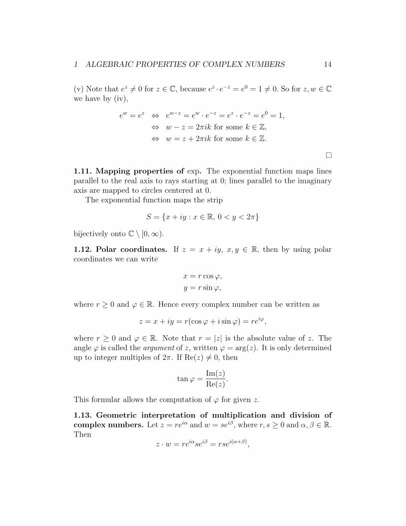
(v) Note that ez 6= 0 for z ∈ C, because ez · e−z = e0 = 1 6= 0. So for z, w ∈ Cwe have by (iv),
ew = ez ⇔ ew−z = ew · e−z = ez · e−z = e0 = 1,
⇔ w − z = 2πik for some k ∈ Z,⇔ w = z + 2πik for some k ∈ Z.
1.11. Mapping properties of exp. The exponential function maps linesparallel to the real axis to rays starting at 0; lines parallel to the imaginaryaxis are mapped to circles centered at 0.
The exponential function maps the strip
S = x+ iy : x ∈ R, 0 < y < 2π
bijectively onto C \ [0,∞).
1.12. Polar coordinates. If z = x + iy, x, y ∈ R, then by using polarcoordinates we can write
x = r cosϕ,
y = r sinϕ,
where r ≥ 0 and ϕ ∈ R. Hence every complex number can be written as
z = x+ iy = r(cosϕ+ i sinϕ) = reiϕ,
where r ≥ 0 and ϕ ∈ R. Note that r = |z| is the absolute value of z. Theangle ϕ is called the argument of z, written ϕ = arg(z). It is only determinedup to integer multiples of 2π. If Re(z) 6= 0, then
tanϕ =Im(z)
Re(z).
This formular allows the computation of ϕ for given z.
1.13. Geometric interpretation of multiplication and division ofcomplex numbers. Let z = reiα and w = seiβ, where r, s ≥ 0 and α, β ∈ R.Then
z · w = reiαseiβ = rsei(α+β),

1 ALGEBRAIC PROPERTIES OF COMPLEX NUMBERS 15
andz
w=reiα
seiβ=r
seiαe−iβ =
r
sei(α−β), w 6= 0.
So complex numbers are mutliplied by mutiplying their absolute values andadding their arguments. One divides them by dividing their absolute valuesand subtracting their arguments.
These facts and their geometric interpretations will be used throughout;for example, multiplication by i = eiπ/2, i.e., the map z ∈ C 7→ iz correspondto counterclockwise rotation in the plane by 90o.
1.14. Computation of nth roots. For z ∈ C and n ∈ N we set
zn := z · · · z︸ ︷︷ ︸n factors
.
We use the convention z0 := 1 for z ∈ C, and set zn := (z−1)|n| for n ∈ Z,n < 0, z 6= 0. One then has the usual computational rules
znzk = zn+k,
(zn)k = znk,
(zw)n = znwn
for z, w ∈ C, z, w 6= 0, n, k ∈ Z.Now let n ∈ N, a ∈ C, a 6= 0. Every solution z of the equation zn = a
(for given n and a) is called an nth root of a. As we will see momentarily,every a 6= 0 has precisely n distinct nth roots; hence for complex numbersa we will usually not use the ambiguous notation n
√a, but we will use it for
positive real numbers a (where it denotes the unique positive real numberwith ( n
√a)n = a).
We write a = reiϕ with r > 0, ϕ ∈ R, and use the ansatz z = ρeiα, whereρ > 0 and α ∈ R. Then
zn = z · · · z︸ ︷︷ ︸n factors
= ρneinα = reiϕ.
Hence ρn = r and nα = ϕ+ 2πk for k ∈ Z. This implies ρ = n√r and
α =ϕ
n+
2π
nk, k ∈ Z.
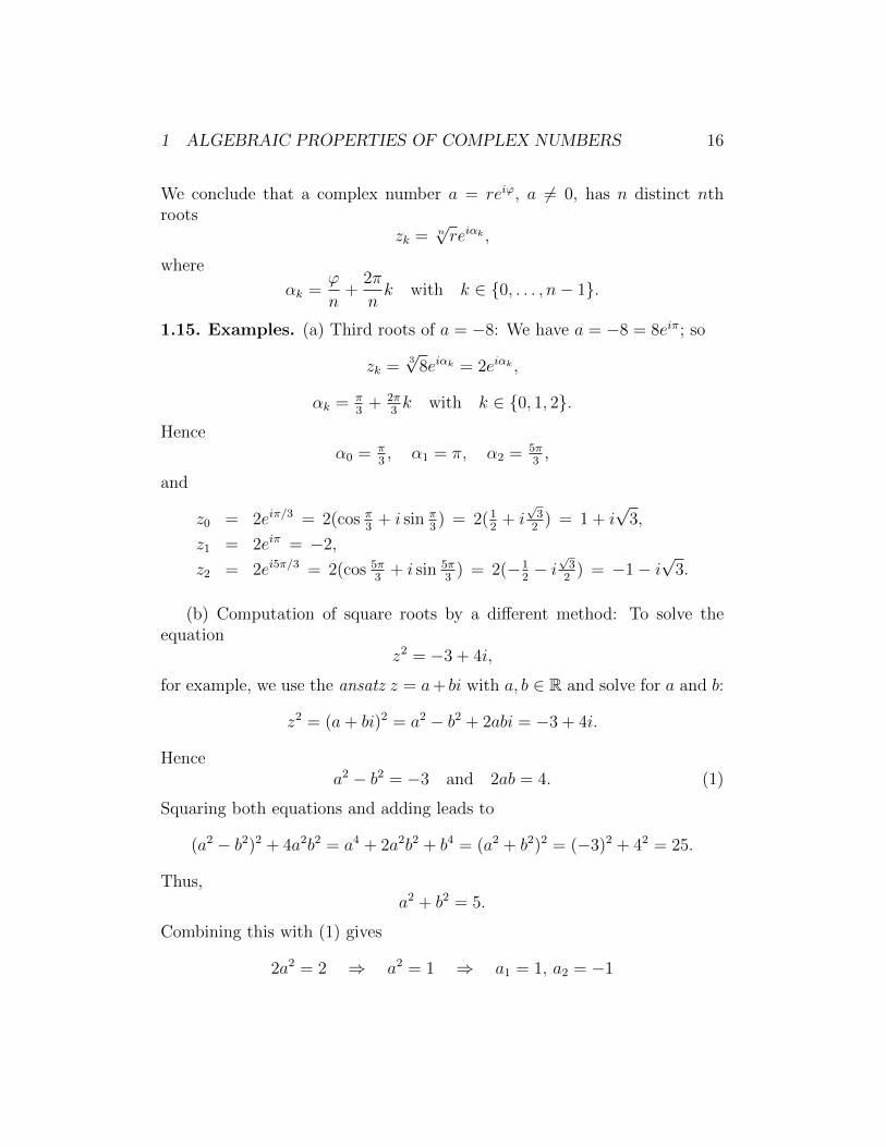
1 ALGEBRAIC PROPERTIES OF COMPLEX NUMBERS 16
We conclude that a complex number a = reiϕ, a 6= 0, has n distinct nthroots
zk = n√reiαk ,
where
αk =ϕ
n+
2π
nk with k ∈ 0, . . . , n− 1.
1.15. Examples. (a) Third roots of a = −8: We have a = −8 = 8eiπ; so
zk =3√
8eiαk = 2eiαk ,
αk = π3
+ 2π3k with k ∈ 0, 1, 2.
Henceα0 = π
3, α1 = π, α2 = 5π
3,
and
z0 = 2eiπ/3 = 2(cos π3
+ i sin π3) = 2(1
2+ i
√3
2) = 1 + i
√3,
z1 = 2eiπ = −2,
z2 = 2ei5π/3 = 2(cos 5π3
+ i sin 5π3
) = 2(−12− i
√3
2) = −1− i
√3.
(b) Computation of square roots by a different method: To solve theequation
z2 = −3 + 4i,
for example, we use the ansatz z = a+ bi with a, b ∈ R and solve for a and b:
z2 = (a+ bi)2 = a2 − b2 + 2abi = −3 + 4i.
Hencea2 − b2 = −3 and 2ab = 4. (1)
Squaring both equations and adding leads to
(a2 − b2)2 + 4a2b2 = a4 + 2a2b2 + b4 = (a2 + b2)2 = (−3)2 + 42 = 25.
Thus,a2 + b2 = 5.
Combining this with (1) gives
2a2 = 2 ⇒ a2 = 1 ⇒ a1 = 1, a2 = −1
1 ALGEBRAIC PROPERTIES OF COMPLEX NUMBERS 17
andb1 = 2, b2 = −2.
So we get the solutions
z1 = 1 + 2i and z2 = −1− 2i.
Note that z2 = −z1 as it should be.
(c) Solutions of quadratic equations can be computed as usual by complet-ing the square, etc. A more general fact is true: Every polynomial equation
zn + an−1zn−1 + · · ·+ a1z + a0 = 0,
where a0, . . . , an−1 ∈ C has a solution z ∈ C. This Fundamental Theorem ofAlgebra will be proved later in this course.
2 Topological properties of CIn this section we summarize some standard facts from point-set topology.We will mostly omit proofs or only give a brief outline.
Definition 2.1. A metric space (X, d) is a set X together with a functiond : X ×X → [0,∞) such that for all x, y, z ∈ X the following properties aretrue:
(i) d(x, y) = 0 iff x = y,
(ii) d(x, y) = d(y, x) (symmetry),
(iii) d(x, z) ≤ d(x, y) + d(y, z) (triangle inequality).
If these axioms hold, then d is called a metric on X.In a metric space (X, d) we define for a ∈ X and r > 0,
B(a, r) := x ∈ X : d(x, a) < r,B(a, r) := x ∈ X : d(x, a) ≤ r,
and call this the open ball and the closed ball of radius r centered at a,respectively.
Often one also calls B(a, r) the (open) r-neighborhood of a.
Example 2.2. If we define d(z, w) := |z−w| for z, w ∈ C, then d is a metricon C, called the Euclidean metric. From now on we consider C as a metricspace equipped with the Euclidean metric.
Definition 2.3. Let (X, d) be a metric space, and M ⊆ X. A point x ∈ Xis called
(i) an interior point of M if there exists ε > 0 such that B(x, ε) ⊆M ,
(ii) an exterior point of M if there exists ε > 0 such that B(x, ε) ⊆ X \M .
(iii) a boundary point of M if M ∩ B(x, ε) 6= ∅ and (X \M) ∩ B(x, ε) 6= ∅for all ε > 0.
The set of interior points of M is denoted by int(M), and the set ofboundary points by ∂M .
18
2 TOPOLOGICAL PROPERTIES OF C 19
Remark 2.4. Every point in X is an interior point, an exterior point, or aboundary point of M , and these cases are mutually exclusive. An interiorpoint of M always belongs to M , while an exterior point always lies in thecomplement of M in X. A boundary point of M may or may not belong toM .
Definition 2.5. Let (X, d) be a metric space, and M ⊆ X. Then M is calledopen if it has only interior points, i.e., for all x ∈ M there exists ε > 0 suchthat B(x, ε) ⊆M .
The set M is called closed if it contains all of its boundary points.
Example 2.6. D := z ∈ C : |z| < 1 is an open set in C, called the openunit disk. The set D := z ∈ C : |z| ≤ 1 is a closed set in C, called theclosed unit disk. The set M = D ∪ 1 is neither open nor closed.
Definition 2.7. Let (X, d) be a metric space, and M ⊆ X. Then M :=M ∪ ∂M is called the closure of M .
One can show that M is the smallest closed set in X containing M .Our notation for the closed unit disk D was motivated by the fact that
this set is the closure of D.
Theorem 2.8. Let (X, d) be a metric space. Then the following statementsare true:
(i) a set in X is
open
closed
if its complement is
closedopen
,
(ii)
a union
an intersection
of a family of
open
closed
sets in X is
open
closed
,
(iii)
an intersection
a union
of a finite family of
open
closed
sets in X is
open
closed
.
Remark 2.9. Suppose X is a set together with a family O of its subsetscalled open sets. If ∅, X ∈ O and if the properties (ii) and (iii) in the previoustheorem are satisfied, then (X,O) is called a topological space and the systemO a topology on X.
By what we have seen, every metric d on a set X determines a naturalsystem O of open sets that form a topology on X. One calls this the topologyinduced by d.

2 TOPOLOGICAL PROPERTIES OF C 20
Definition 2.10. Let (X, d) be a metric space, and xn be a sequence ofpoints in X.
(i) The sequence xn is called convergent if there exists a point x ∈ X(the limit of xn) such that for all ε > 0 there exists N ∈ N such thatfor all n ∈ N with n ≥ N we have d(x, xn) < ε.
One can show that if the limit x exists, then it is unique, and one writesx = lim
n→∞xn or simply xn → x.
(ii) The sequence xn is called a Cauchy sequence if for all ε > 0 thereexists N ∈ N such that for all n, k ∈ N with n, k ≥ N we haved(xn, xk) < ε.
(iii) A point x ∈ X is called a sublimit of xn if there exists a subsequencexnk of xn such that lim
k→∞xnk
= x. In this case, we say that xnsubconverges to x.
Proposition 2.11. A sequence zn in C converges if and only if the se-quences Re(zn) and Im(zn) of real numbers converge.
In case of convergence we have
limn→∞
zn = limn→∞
Re(zn) + i limn→∞
Im(zn).
Proof. ⇒: Suppose zn converges, and let z := limn→∞
zn. Note that |Re(w)| ≤|w| for w ∈ C. Hence
|Re(zn)− Re(z)| ≤ |zn − z|
for n ∈ N. This implies that limn→∞
Re(zn) = Re(z). Similarly, limn→∞
Im(zn) =
Im(z).
⇐: Suppose Re(zn) and Im(zn) converge. Let a := limn→∞
Re(zn),
b := limn→∞
Im(zn), and z := a+ bi. Note that for all w ∈ C we have
|w| =√
Re(w)2 + Im(w)2 ≤ |Re(w)|+ | Im(w)|.
Hence|zn − z| ≤ |Re(zn)− a|+ | Im(zn)− b|.
It follows that limn→∞
zn = z.
2 TOPOLOGICAL PROPERTIES OF C 21
Remark 2.12. The usual computational rules for limits are true for se-quences in C. If zn and wn are sequences in C with zn → z and wn → w,then
(i) zn + wn → z + w,
(ii) znwn → zw,
(iii) Re(zn)→ Re(z), Im(zn)→ Im(z), zn → z, |zn| → |z|,
(iv)wnzn→ w
z, if, in addition, z 6= 0 and zn 6= 0 for n ∈ N.
Definition 2.13. A metric space (X, d) is called complete if every Cauchysequence in X converges.
Theorem 2.14. The space C (equipped with the Euclidean metric) is com-plete.
Proof. This follows from the completeness of R and Proposition 2.11.
Proposition 2.15. A subset A of a metric space (X, d) is closed if and onlyif every convergent sequence in A has its limit also in A.
Definition 2.16. A subset K of a metric space (X, d) is called compact ifevery open cover of K has a finite subcover; i.e., whenever Ui : i ∈ I is afamily of open sets in X with K ⊆
⋃i∈I Ui, then there exist i1, . . . , in ∈ I
such that K ⊆ Ui1 ∪ · · · ∪ Uin .
Theorem 2.17. Let (X, d) be a metric space. Then K ⊆ X is compact ifand only if every sequence xn in K has a sublimit in K, i.e., there existsa subsequence xnk
of xn that converges and x = limn→∞
xn ∈ K.
The last condition is called sequential compactness. So a set in a metricspace is compact if and only if it is sequentially compact.
Proposition 2.18. (a) Every compact metric space is complete.
(b) Every compact subset of a metric space is closed.
Theorem 2.19 (Heine-Borel). A subset K ⊆ C is compact if and only if itis closed and bounded.

2 TOPOLOGICAL PROPERTIES OF C 22
Remark 2.20. A subset M of a metric space is called bounded if its diameterdefined as
diam(M) := supd(x, y) : x, y ∈M
is finite. This is equivalent to the requirement that there exists a ∈ X andr > 0 such that M ⊆ B(a, r).
Definition 2.21. Let (X, d) and (Y, ρ) be metric spaces, and f : X → Y bea map.
(i) We say that f approaches the limit y ∈ Y as x approaches a ∈ X,written as lim
x→af(x) = y, if for all ε > 0 there exists δ > 0 such that for
all x ∈ X we have that
0 < d(x, a) < δ implies ρ(f(x), y) < ε.
(ii) The map f is called continuous at a ∈ X if limx→a
f(x) = f(a).
(iii) The map f is called continuous (on X) if it is continuous at all pointsa ∈ X.
Note that in (i) it does not matter what happens for x = a.
Proposition 2.22. Let (X, d) and (Y, ρ) be metric spaces, and f : X → Ybe a map. Then the following condition are equivalent:
(i) f is continuous,
(ii) for every convergent sequence xn in X, the sequence f(xn) alsoconverges and we have
limn→∞
f(xn) = f(
limn→∞
xn),
(iii) for all x ∈ X and all ε > 0 there exists δ > 0 such that
f(B(x, δ)) ⊆ B(f(x), ε),

2 TOPOLOGICAL PROPERTIES OF C 23
(iv) preimages of open sets are open, i.e., f−1(V ) is open in X wheneverV ⊆ Y is open in Y .
(v) preimages of closed sets are closed.
Remark 2.23. We will be mostly interested in limits of functions f : M → C,where M ⊆ R or M ⊆ C. In this case, one has the usual computational rulesfor function limits. For example, if f : M → C and g : M → C are functions,and a ∈M , then
limx→a
f(x)g(x) =(limx→a
f(x))(
limx→a
g(x))
if the limits on the right hand side exist, etc. Based on this one can provethat if f : M → C and g : M → C are continuous, then f + g is continuous,fg is continuous, etc.
Theorem 2.24. Let (X, d) and (Y, ρ) be metric spaces, and f : X → Ybe a continuous map. If K ⊆ X is compact, then f(K) ⊆ Y is compact(continuous images of compact sets are compact).
Proof. Suppose that K ⊆ X is compact, and let yn be an arbitrary se-quence in f(K). Then for all n ∈ N there exists xn ∈ K such that yn = f(xn).Then xn is a sequence in K. Since K is compact, by Theorem 2.17 thesequence xn has a convergent subsequence xnk
with a limit in K, sayxnk→ x ∈ K. By continuity of f it follows that
ynk= f(xnk
)→ f(x) ∈ f(K).
So yn has a sublimit in f(K). Hence f(K) is compact by Theorem 2.17.
Remark 2.25. There are other important statements involving compactnessand continuity: a real-valued function f : X → R on a compact metric space(X, d) attains maximum and minimum. A continuous map f : X → Y be-tween a compact metric space (X, d) and a metric space (Y, ρ) is uniformlycontinuous, i.e., for all ε > 0 that exists δ > 0 such that for all x, y ∈ X wehave that
d(x, y) < δ implies ρ(f(x), f(y)) < ε.
Definition 2.26. A subset M of a metric space (X, d) is called connected ifthe following condition is true: if U, V ⊆ X are open sets with M ⊆ U ∪ Vand U ∩ V = ∅, then M ⊆ U or M ⊆ V .

2 TOPOLOGICAL PROPERTIES OF C 24
Remark 2.27. (a) For M = X this statement can be reformulated in equiv-alent form in the following way: a metric space X is connected if everydecomposition X = U ∪V , U ∩V = ∅, into open subsets U, V ⊆ X is trivial,i.e., U = M or V = M . Equivalently, X is connected if ∅ and X are the onlysubsets of X that are both open and closed.
(b) For subsets M of a metric space (X, d) one can characterize connected-ness in a similar way if one uses relatively closed and open sets. By definitiona set A ⊆M is called relatively closed or relatively open in M if there existsa closed or an open set B ⊆ X, respectively, such that A = B ∩M .
The restriction dM := d|M ×M of d to M is a metric on M . It is nothard to see that A ⊆ M is relatively closed or relatively open in M if A isclosed or open in the metric space (M,dM), respectively.
Using this terminology one can show that a subset M of a metric spaceis connected if and only if ∅ and M are the only subsets of M that are bothrelatively closed and relatively open in M (exercise!).
Proposition 2.28. A non-empty subset M ⊆ R is connected if and only ifM is an interval (possibly degenerate).
Here we call an interval degenerate if it consists of only one point. Allintervals in R are of the form [a, b], [a, b), (a, b], (a, b), (−∞, a], (−∞, a),[a,+∞), (a,+∞), or (−∞,+∞) = R, where a, b ∈ R, a ≤ b.
Proposition 2.29. Let (X, d) and (Y, ρ) be metric spaces, and f : X → Ybe a continuous map. If M ⊆ X is connected, then f(M) ⊆ Y is connected(continuous images of connected sets are connected).
Proof. Under the given assumptions, assume that M ⊆ X is connected. Toshow that f(M) is connected, let U, V ⊆ Y be arbitrary open sets withf(M) ⊆ U ∪ V and U ∩ V = ∅. Since f is continuous, the sets U ′ := f−1(U)and V ′ := f−1(V ) are open. Moreover,
U ′ ∪ V ′ = f−1(U) ∪ f−1(V ) = f−1(U ∪ V ) ⊇ f−1(f(M)) ⊇M,
andU ′ ∩ V ′ = f−1(U) ∩ f−1(V ) = f−1(U ∩ V ) = f−1(∅) = ∅.
Since M is connected, we have M ⊆ U ′ or M ⊆ V ′, say M ⊆ U ′. Then
f(M) ⊆ f(U ′) = f(f−1(U)) ⊆ U.
Hence f(M) is connected.
2 TOPOLOGICAL PROPERTIES OF C 25
Definition 2.30. A non-empty set Ω ⊆ C is called a region if it is open andconnected.
Theorem 2.31. A non-empty open set Ω ⊆ C is a region if and only if anytwo points a, b ∈ Ω can be joined by a polygonal path in Ω.
If z, w ∈ C we denote by
[z, w] := (1− t)z + tw : t ∈ [0, 1]
the closed line segment with endpoints z and w. A polygonal path P in C isa set of the form
P = [z0, z1] ∪ · · · ∪ [zn−1, zn],
where n ∈ N, z1, . . . , zn ∈ C. Such a path joins two points z and w if z0 = zand w = zn.
Proof. ⇒: Assume that Ω is a region. Fix a point a ∈ Ω, and consider thepoints set M of points b ∈ Ω that can be joined to a by a polygonal path inΩ. It suffices to show that M = Ω.
Note that a ∈M , and so M 6= ∅. In order to conclude that M = Ω, it isenough to show that M is open and relatively closed in Ω.
1. M is open.If y ∈ M ⊆ Ω, then, since Ω is open, there exists ε > 0 such that
B(y, ε) ⊆ Ω. If z ∈ B(y, ε) we can find a polygonal path in Ω joining aand z as a union of a polygonal path joining a and y and the line segment[y, z] ⊆ B(y, ε) ⊆ Ω. Hence B(y, ε) ⊆M , and so M is open.
2. M is relatively closed.Let xn be an arbitrary sequence in M that converges in the “ambient”
space Ω. So xn → x ∈ Ω. We have to show that x ∈M .Since Ω is open, there exists ε > 0 such that B(x, ε) ⊆ Ω. Since xn → x,
there exists k ∈ N such that xk ∈ B(x, ε). Now xk ∈M and [xk, x] ⊆ B(x, ε).So we can find a polygonal path in Ω joining a and x by first joining a andxk by a polygonal path in Ω followed by the line segment [xk, x]. So x ∈M ,and M is relatively closed.⇐: Suppose any two points in Ω can be joined by a polygonal path in
Ω. Fix a ∈ Ω. Then for every point b ∈ Ω there exists a polygonal pathPb ⊆ Ω joining a and b. Then Ω =
⋃b∈Ω Pb and a ∈
⋂b∈Ω Pb. Moreover, each
polygonal path is the image of an interval in R and hence connected.We conclude that Ω is connected, because a union of a family of connected
sets with non-empty intersection is connected (exercise!).
3 Differentiation
Remark 3.1. An obvious extension of differential calculus of real-valuedfunctions of one real variable is to complex-valued functions of one real vari-able; so if f : I → C is a complex-valued function on an interval I ⊆ R, wecall f differentiable at x0 ∈ I, if the limit
limx∈x0
f(x)− f(x0)
x− x0
exists. This limit is denoted by f ′(x0) and called the derivative of f at x0.It (essentially) follows from Proposition 2.11 that f is differentiable at x0
if and only if the functions Re(f) and Im(f) are differentiable at x0. In thiscase
f ′(x0) = (Re(f))′(x0) + i(Im(f))′(x0).
For example, let f : R → C, f(x) := eix for x ∈ R. Then f(x) =cosx+ i sinx, and so
f ′(x) = − sinx+ i cosx
= i(cosx+ i sinx) = ieix.
One is tempted to use the chain rule here:
d
dxeix =
dez
dz
∣∣∣∣z=ix
· d(ix)
dx= ez|z=ix · i = ieix.
At the moment this is not justified, because we have not yet defined deriva-tives of complex-valued functions of a complex variable.
Definition 3.2. Let U ⊆ C be open, and f : U → C be a function.
(i) f is called differentiable at z0 ∈ U if
limz→z0
f(z)− f(z0)
z − z0
exists. This limit is called the derivative of f at z0 and denoted by
f ′(z0),df
dz(z0), etc.
26
3 DIFFERENTIATION 27
(ii) f is called holomorphic (on U) if it is differentiable at every pointz0 ∈ U .
(iii) We denote by H(U) the set of all holomorphic functions on U .
Theorem 3.3. Let U, V ⊆ C be open sets.
(a) If f ∈ H(U), then f is continuous on U .
(b) Let a, b ∈ C, and f, g ∈ H(U). Then
(i) af + bg ∈ H(U), and (af + bg)′ = af ′ + bg′,
(ii) fg ∈ H(U) and (fg)′ = f ′g + fg′ (product rule),
(iii)f
g∈ H(U) and
(f
g
)′=f ′g − fg′
g2if we assume in addition that
g(z) 6= 0 for z ∈ U (quotient rule).
(c) Let f ∈ H(U), g ∈ H(V ), and f(U) ⊆ V . Then g f ∈ H(U) and(g f)′ = (g′ f) · f ′ (chain rule).
Proof. The standard proofs from real analysis transfer to this setting. Forillustration we will prove (a) and (c).
(a) Let z0 ∈ U be arbitary. Then
limz→z0
(f(z)− f(z0)) = limz→z0
f(z)− f(z0)
z − z0
(z − z0)
=
(limz→z0
f(z)− f(z0)
z − z0
)·(
limz→z0
(z − z0)
)= f ′(z0) · 0 = 0.
Hencelimz→z0
f(z) = f(z0),
and so f is continuous at z0.(c) A function h : W → C on an open set W ⊆ C is differentiable at
z0 ∈ W if and only if there exists a constant c ∈ C, and a function s : W → Cwith lim
z→z0s(z) = 0 such that
h(z)− h(z0) = (z − z0)(c+ s(z))

3 DIFFERENTIATION 28
for all z ∈ W . If this is true, then c = h′(z0).Now suppose f and g are as in the statement, and let z0 ∈ U be arbitrary.
Set w0 = f(z0). Then there exist functions s : U → C and t : V → C withlimz→z0
s(z) = 0 and limw→w0
t(w) = 0 such that
f(z)− f(z0) = (z − z0)(f ′(z0) + s(z)), z ∈ U,g(w)− g(w0) = (w − w0)(g′(w0) + t(w)), w ∈ V.
Hence for all z ∈ U we have
g(f(z)︸︷︷︸w
)− g(f(z0)︸ ︷︷ ︸w0
) = (f(z)− f(z0))(g′(w0) + t(f(z))
),
= (z − z0)(f ′(z0) + s(z)
)(g′(w0) + t(f(z))
)= (z − z0)
(g′(w0)f ′(z0) + g′(w0)s(z) + f ′(z0)t(f(z)) + s(z)t(f(z))︸ ︷︷ ︸
r(z)
).
Note that f(z)→ f(z0) = w0 as z → z0 by continuity of f , and so
limz→z0
r(z) = limz→z0
(g′(w0)s(z) + f ′(z0)t(f(z)) + s(z)t(f(z))
)= g′(w0) lim
z→z0s(z) + f ′(z0) lim
w→w0
t(w) +(
limz→z0
s(z))(
limw→w0
t(w))
= g′(w0) · 0 + f ′(z0) · 0 + 0 · 0 = 0.
Hence g f is differentiable at z0 and
(g f)′(z0) = g′(w0)f ′(z0) = g′(f(z0))f ′(z0).
The claim follows.
Remark 3.4. Similar statements hold for complex-valued functions on in-tervals. One can also prove a chain rule for a function given by a (post-)composition of a complex-valued function on interval by a holomorphic func-tion.
Theorem 3.5. Let Ω ⊆ C be a region, and f ∈ H(Ω). If f ′ = 0, then f isa constant function.
Proof. Fix z0 ∈ Ω. We will show that f(z) = f(z0) for all z ∈ Ω.
3 DIFFERENTIATION 29
Let z ∈ Ω be arbitrary. By Theorem 2.31 there exists a polygonal path
P = [z0, z1] ∪ · · · ∪ [zn−1, zn] ⊆ Ω,
where zn = z. So it is enough to show that f is constant on each segment[u, v] ⊆ Ω.
To see this, let u, v ∈ Ω be arbitrary, and consider h : [0, 1]→ C, h(t) :=f(u+ (v − u)t) for t ∈ [0, 1]. Then by the chain rule,
h′(t) = f ′(u+ (v − u)t)(v − u) = 0
for all t ∈ [0, 1]. Hence h is constant on [0, 1], and so f is constant on[u, v].
Remark 3.6. By using the previous statements, one can produce a certain,although limited, supply of holomorphic functions; namely, it follows fromthe definitions that a constant function z 7→ c ∈ C, and the function z 7→ zare holomophic in C, and we have
dc
dz= 0 and
dz
dz= 1.
By induction it follows from the product rule that z 7→ zn is holomorphic inC for all n ∈ N, and
dzn
dz= nzn−1.
This implies that each polynomial P , i.e., each function P : C → C of theform
z 7→ P (z) := a0 + a1z + · · ·+ anzn,
where n ∈ N0, a0, . . . , an ∈ C, is holomorphic on C. Finally, every rationalfunction
R(z) =P (z)
Q(z),
where P and Q 6= 0 are polynomials, is holmorphic on the complementC \Q−1(0) of the zero-set of Q.
Remark 3.7. For the rest of this section we identify C with R2 by thecorrespondence z = x + iy ∈ C ∼= (x, y) ∈ R2. We write a complex-valuedfunction f : U → C on U ⊆ C in the form f = u+ iv, where u = Re(f) and
3 DIFFERENTIATION 30
v = Im(f). Then u and v are considered as functions of (x, y) ∈ U ⊆ R2,and we have
f(x+ iy) = u(x, y) + iv(x, y),
where x+ iy ∼= (x, y) ∈ U .
We will denote by ux, uy, . . . partial derivatives; so ux =∂u
∂x, etc.
Theorem 3.8. Let U ⊆ C be open, f : U → C, f = u+ iv.Then f is holomorphic on U if and only if u and v are C1-smooth on U
and the so-called Cauchy-Riemann equations
ux = vy, uy = −vx
are valid on U .In this case,
f ′(x+ iy) = ux(x, y) + ivx(x, y)
=1
i(uy(x, y) + ivy(x, y)),
whenever x+ iy ∈ U .
For the proof of the implication ⇒ we will use the following
Fact: If U ⊆ C is open, and f ∈ H(U), then f ′ ∈ H(U).
This will be proved later in this course (independently of the previoustheorem of course).
Proof. ⇒: Suppose f is holomorphic on U . Then for each z = x + iy ∈ Uwe have,
f ′(z) = limw→0
f(z + w)− f(z)
w.
Setting w = h or w = ik, where h, k ∈ R, and h→ 0 or k → 0, we obtain
f ′(x+ iy) = limh→0
f(z + h)− f(z)
h
= limh→0
u(x+ h, y)− u(x, y)
h+ i lim
h→0
v(x+ h, y)− v(x, y)
h= ux(x, y) + ivx(x, y),
3 DIFFERENTIATION 31
and
f ′(x+ iy) = limk→0
f(z + ik)− f(z)
ik
=1
ilimk→0
u(x, y + k)− u(x, y)
k+
1
i· i lim
k→0
v(x, y + k)− v(x, y)
k
=1
i(uy(x, y) + ivy(x, y)).
In particular, the partial derivatives of u and v exist, and
ux + ivx =1
i(uy + ivy) = vy − iuy
on U ; so ux = vy and vx = −uy.Moreover, we have that
ux = Re(f ′), vx = Im(f ′), uy = − Im(f ′), vy = Re(f ′).
Since by the fact mentioned above, f ′ is holomorphic and hence continuouson U , the partial derivatives of u and v are also continuous on U . It followsthat u and v are C1-smooth.
⇐: Suppose that u and v are C1-smooth and that the Cauchy-Riemannequations hold. Since the functions u and v are C1-smooth, they are differ-entiable on U ; this means that for each point (x, y) ∈ U and (h, k) ∈ R2 with|(h, k)| :=
√h2 + k2 small we have
u(x+ h, y + k) = u(x, y) + ux(x, y)h+ uy(x, y)k + r(h, k),
v(x+ h, y + k) = v(x, y) + vx(x, y)h+ vy(x, y)k + s(h, k),
wherer(h, k)
|(h, k)|→ 0 and
s(h, k)
|(h, k)|→ 0
as |(h, k)| → 0.If we set z = x + iy, w = h + ik, and c = ux(x, y) + ivx(x, y), then for
3 DIFFERENTIATION 32
small |w| 6= 0, we have by the Cauchy-Riemann equations,∣∣∣∣f(z + w)− f(z)
w− c∣∣∣∣ =
∣∣∣∣f(z + w)− f(z)− (h+ ik)c
w
∣∣∣∣=
1
|w|∣∣f(z + w)− f(z)− hux(x, y)− ihvx(x, y)− kuy(x, y)− ikvy(x, y)
∣∣≤ 1
|w|∣∣u(x+ h, y + k)− u(x, y)− hux(x, y)− kuy(x, y)
∣∣+1
|w|∣∣v(x+ h, y + k)− v(x, y)− hvx(x, y)− kvy(x, y)
∣∣≤ |r(h, k)|+ |s(h, k)|
|(h, k)|→ 0 as w = h+ ik → 0.
It follows that f is differentiable at z. Since z ∈ U was arbitrary, f isholomorphic on U .
Example 3.9. By using the previous theorem, one can see that the expo-nential function is holomorphic on X; indeed,
ez = ex+iy = ex cos y + iex sin y,
and sou(x, y) = ex cos y and v(x, y) = ex sin y.
Hence u and v are C1-smooth in R2. Moreover, we have
ux = ex cos y = vy and uy = −ex sin y = −vx,
and so the Cauchy-Riemann equations hold.For the derivative of the exponential function we obtain
d
dzez = ux + ivx = ex cos y + iex sin y = ez.
Remark 3.10. If f = u + iv is holomorphic, then u and v are C1-smoothand the first partial derivatives of u and v are again real and imaginary partsof a holomorphic function (ux = Re(f ′), etc.). It follows that the first partialderivatives of u and v are C1-smooth, and so u and v are C2-smooth. If werepeat this argument, we conclude that u and v are C∞-smooth.

3 DIFFERENTIATION 33
Definition 3.11. Let U ⊆ R2 be open, and h : U → R be C2-smooth. TheLaplacian ∆h of h is defined as
∆h = hxx + hyy =∂2h
∂x2+∂2h
∂y2.
The function h is called harmonic on U if its Laplacian vanishes on U ,i.e., if ∆h = 0 on U .
Theorem 3.12. Let U ⊆ C be open, f ∈ H(U), f = u + iv. Then u and vare harmonic on U .
Proof. The functions u and v are C∞-smooth by Remark 3.10. Moreover,ux = vy and uy = −vx by the Cauchy-Riemann equations. Hence
∆u = uxx + uyy = vyx − vxy = 0,
∆v = vxx + vyy = −uyx + uxy = 0.
Remark 3.13. If f = u+iv is a complex-valued function of (x, y) ∈ U ⊆ R2,one defines its partial derivatives as
∂f
∂x:=
∂u
∂x+ i
∂v
∂x, and
∂f
∂y:=
∂u
∂y+ i
∂v
∂y.
Usually, it is better to work with the so-called z- and z-derivatives or Wirtingerderivatives defined as
∂f
∂z:=
1
2
(∂f
∂x− i∂f
∂y
), and
∂f
∂z:=
1
2
(∂f
∂x+ i
∂f
∂y
).
So symbolically,
∂
∂z=
1
2
(∂
∂x− i ∂
∂y
), and
∂
∂z=
1
2
(∂
∂x+ i
∂
∂y
).
Note that
∂z
∂z=
1
2
(∂(x+ iy)
∂x− i∂(x+ iy)
∂y
)=
1
2(1 + 1) = 1,
∂z
∂z=
1
2
(∂(x− iy)
∂x− i∂(x− iy)
∂y
)=
1
2(1− 1) = 0.
3 DIFFERENTIATION 34
Similarly,∂z
∂z= 0 and
∂z
∂z= 1.
So with respect to the operator∂
∂zthe function z 7→ z behaves as expected,
and z 7→ z like a constant, and we have a similar behavior for the operator∂
∂z.
Moreover, the usual computational rules hold for these operators (productrule, quotient rule, etc.). This allows computations such as
∂|z|2
∂z=∂(zz)
∂z=∂z
∂zz +
∂z
∂zz = z.
We also have a version of the chain rule: suppose that h = h(w, w) andw = w(z, z). Then
∂h
∂z=∂h
∂w· ∂w∂z
+∂h
∂w· ∂w∂z
, and∂h
∂z=∂h
∂w· ∂w∂z
+∂h
∂w· ∂w∂z
.
Note also (∂w
∂z
)=∂w
∂z, and
(∂w
∂z
)=∂w
∂z.
Theorem 3.14. Let U ⊆ C be open, f : U → C, f = u + iv. Then f isholomorphic on U if and only if f is C1-smooth (i.e., u and v are C1-smooth)and
∂f
∂z= 0
on U (complex version of the Cauchy-Riemann equations).
In this case, f ′ =∂f
∂z.
Proof. We have
∂f
∂z=
1
2(fx + ify) =
1
2(ux + ivx) +
i
2(uy + ivy)
=1
2(ux − vy) +
i
2(vx + uy).
So the condition∂f
∂z= 0 is equivalent to the Cauchy-Riemann equations.
The first part of the statement follows from Theorem 3.8.
3 DIFFERENTIATION 35
In case of holomorphicity we have
f ′ = ux + ivx =1
i(uy + ivy).
Hence
f ′ =1
2(ux + ivx)−
i
2(uy + ivy) =
∂u
∂z+ i
∂v
∂z=∂f
∂z.
Example 3.15. Let f(z) = z|z|2 for z ∈ C. Is f anywhere holomorphic inC? Obviously, f ∈ C∞(C), and we have
∂f
∂z=∂(z2z)
∂z= z2.
So the Cauchy-Riemann equations are true only for z = 0. Hence there is noopen set U ⊆ C where f |U is holomorphic.
Definition 3.16. Let U ⊆ C be open, u : U → R be C2-smooth and har-monic. A harmonic function v : U → R is called a harmonic conjugate of uin U if f = u+ iv is holomorphic.
Remark 3.17. (a) It easily follows from the Cauchy-Riemann equationsthat if a harmonic conjugate exists on a region U , then it is unique up to anadditive constant (exercise!).
(b) In general a harmonic conjugate need not exist. If U satisfies a specialgeometric condition, then every harmonic function u on U has a harmonicconjugate. The requirement is that U should have “no holes” and is simplyconnected. This concept will be later discussed in detail in this course.
Example 3.18. (a) Let u(x, y) = x2−y2 for (x, y) ∈ R2. Then u ∈ C∞(R2),ux = 2x, uy = −2y, and uxx = 2, uyy = −2. Hence ∆u = 0, and so u isharmonic.
Does u have a harmonic conjugate, and how to find it? We use theCauchy-Riemann equation that a harmonic conjugate v of u must satisfy:
vx = −uy = 2y, vy = ux = 2x.
By the first equation we have
v(x, y) =
∫2y dx+ C(y) = 2xy + C(y).
3 DIFFERENTIATION 36
Using this, we getvy = 2x+ C ′(y) = ux = 2x.
Hence C ′(y) = 0, and so C(y) ≡ const. =: c ∈ R. So v(x, y) = 2xy+ c. If weset
f(x+ iy︸ ︷︷ ︸z
) := u(x, y) + iv(x, y) = x2 − y2 + 2ixy + c = z2 + c,
then f is indeed holomorphic.(b) Let u(x, y) = 1
2log(x2 + y2) for (x, y) ∈ U := R2 \ 0. Then u ∈
C∞(R2 \ 0),
ux =x
x2 + y2, uy =
y
x2 + y2, uxx =
−x2 + y2
(x2 + y2)2, uyy =
x2 − y2
(x2 + y2)2.
Hence ∆u = 0, and so u is harmonic on U .Does u have a harmonic conjugate v? If so, then
vy = ux =x
x2 + y2,
and so at least locally, where x 6= 0,
v =
∫x
x2 + y2dy + C(x) = arctan(y/x) + C(x).
Thenvx = − y
x2 + y2+ C ′(x) = −uy = − y
x2 + y2,
so C(x) ≡ const. =: c, and
v(x, y) = arctan(y/x) + c
locally near points (x, y) where x 6= 0.If we introduce polar coordinates, and set z = x+ iy = reiϕ, then locally
near points (x, y) where x 6= 0,
v(x, y) = arctan(y/x) + c = ϕ+ c′,
where c′ is locally constant.If u had a harmonic conjugate, then by continuity necessarily
v(x, y) = ϕ+ c′,

3 DIFFERENTIATION 37
for all (x, y) ∈ U ; but there is no well-defined function (x, y) 7→ ϕ on allof U (it exists locally near each point, or on the slit plane C \ (−∞, 0], forexample).
The conclusion is that u has no harmonic conjugate on U ; on a moreintuitive level, u has a locally harmonic conjugate (unique up to constant),but it changes globally by the period 2π if we run around 0 counter-clockwiseonce.
This is an instance of a more general fact: on arbitrary regions U everyharmonic function has a local harmonic conjugate v, but v changes by certainadditive periods if we run around the “holes” of U .
4 Path integrals
Definition 4.1. A path is a continuous map γ : [a, b] → C defined on acompact interval [a, b] ⊆ R. The image or trace of the path is the set γ([a, b])denoted by γ∗. The endpoints of γ are γ(a) and γ(b). The path is a loop ifγ(a) = γ(b). If γ∗ ⊆ U ⊆ C, then we say γ is a path in U .
The path γ is called piecewise smooth if there exists a partition t0 =a < t1 < · · · < tn = b of [a, b] such that γ is differentiable on each interval[tk−1, tk], k ∈ 1, . . . , n, with continuous derivative γ′.
Definition 4.2. Let h : [a, b] → C be a function. We call h (Riemann)integrable if Re(h) and Im(h) are (Riemann) integrable on [a, b]. If h isintegrable, we define∫ b
a
h(t) dt :=
∫ b
a
(Reh)(t) dt+ i
∫ b
a
(Imh)(t) dt.
Proposition 4.3. Let [a, b] ⊆ R be compact interval, f, g, h : [a, b] → C beintegrable functions, and α, β ∈ C. Then the following statements are true:
(a)
∫ b
a
(αf + βg)(t) dt = α
∫ b
a
f(t) dt+ β
∫ b
a
g(t) dt,
(b)
∣∣∣∣∫ b
a
h(t) dt
∣∣∣∣ ≤ ∫ b
a
|h(t)| dt,
(c) if h has a primitive H, i.e., H is differentiable on [a, b] and H ′ = h,then ∫ b
a
h(t) dt = H(b)−H(a).
Proof. The statements (a) and (c) follow from the corresponding statementsfor integrals of real-valued functions if we split the relevant expressions upinto real and imaginary parts.
(b) Assume h = u + iv, where u = Re(h) and v = Im(h). Define α :=∫ bau(t) dt and β :=
∫ bav(t) dt. Then by the Cauchy-Schwarz inequality we
38

4 PATH INTEGRALS 39
have ∣∣∣∣∫ b
a
h(t) dt
∣∣∣∣2 = α2 + β2 =
∫ b
a
(αu(t) + βv(t)
)dt
≤ (α2 + β2)1/2
∫ b
a
(u(t)2 + v(t)2
)1/2dt
=
∣∣∣∣∫ b
a
h(t) dt
∣∣∣∣ · ∫ b
a
|h(t)| dt.
Inequality (b) follows.
Definition 4.4 (Path integrals). Let γ : [a, b] → C be a piecewise smoothpath, and f : γ∗ → C be a continuous function. Then we define the (path)integral of f over γ (denoted by
∫γf(z) dz,
∫γf , etc.), as∫
γ
f(z) dz :=
∫ b
a
f(γ(t))γ′(t) dt.
Example 4.5. Let a ∈ C, r > 0, and
γ(t) = a+ reit, t ∈ [0, 2π].
This is a positively-oriented parametrization of the circle of radius r centeredat a. Let f(z) = (z − a)n, n ∈ Z. Then γ′(t) = ireit, and so∫
γ
(z − a)n dz =
∫ 2π
0
(reit)nireit dt = irn+1
∫ 2π
0
ei(n+1)t dt
=
i
∫ 2π
0
dt = 2πi, n = −1,
irn+1
i(n+ 1)ei(n+1)t
∣∣∣∣2π0
= 0, n 6= −1.
If we run through the circle with different speed (e.g., γ(t) = a + re2πit,t ∈ [0, 1]), or with different orientation (γ(t) = a + re−it, t ∈ [0, 2π]), thenthe integrals are unchanged or change sign, respectively.
4.6. Reparametrization of paths. Let α : [a, b] → C and β : [c, d] → Cbe piecewise smooth paths. Then β is called a reparametrization of α if

4 PATH INTEGRALS 40
there exists a bijection ϕ : [c, d]→ [a, b] such that ϕ and ϕ−1 are C1-smooth,ϕ(c) = a, ϕ(d) = b, and β = α ϕ.
Integrals do not change under reparametrizations: if β is a reparametri-zation of α and f : α∗ = β∗ → C is continous, then∫
β
f =
∫α
f.
Indeed, ∫β
f =
∫β
f(w) dw =
∫ d
c
f(β(s))β′(s) ds
=
∫ d
c
f(α(ϕ(s)))α′(ϕ(s))ϕ′(s) ds (t = ϕ(s))
=
∫ b
a
f(α(t))α′(t) dt =
∫α
f(z) dz =
∫α
f.
The paths α and β are called equivalent if β is a reparametrization of α (thisis indeed an equivalence relation for paths!).
The oriented interval [a, b] for a, b ∈ C is the path γ : [0, 1]→ C, γ(t) :=(1 − t)a + tb, t ∈ [0, 1] (or any equivalent path). In this case, one writes∫
[a,b]f(z) dz instead of
∫γf(z) dz.
4.7. Computational rules for path integrals. (a) Let γ : [a, b] → C bea piecewise smooth path, f, g : γ∗ → C be continuous, and c, d ∈ C. Then∫
γ
(cf(z) + dg(z)
)dz = c
∫γ
f(z) dz + d
∫γ
g(z) dz.
(b) Suppose γ1 and γ2 are piecewise smooth paths such that the endpointof γ1 is equal to the initial point of γ2. Then we may without loss of generalityassume that γ1 : [0, 1] → C, γ2 : [1, 2] → C and γ1(1) = γ2(1). Then theconcatenation of γ1 and γ2 is the path γ : [0, 2]→ C defined as
γ(t) =
γ1(t), t ∈ [0, 1],γ2(t), t ∈ [1, 2].
If f : γ∗1 ∪ γ∗2 → C is continuous, then∫γ
f(z) dz =
∫γ1
f(z) dz +
∫γ2
f(z) dz.

4 PATH INTEGRALS 41
(c) Let U ⊆ C be open, γ : [a, b] → U be a piecewise smooth path, andf : U → C be a continuous function.
If f has a primitive F , i.e., F ∈ H(U) and F ′ = f , then∫γ
f(z) dz = F (γ(b))− F (γ(a)).
In particular,
∫γ
f(z) dz = 0 if γ is a loop. Indeed,
d
dtF (γ(t)) = F ′(γ(t))γ′(t) = f(γ(t))γ′(t),
and so∫γ
f(z) dz =
∫ b
a
f(γ(t))γ′(t) dt = F (γ(t))
∣∣∣∣ba
= F (γ(b))− F (γ(a)).
4.8. Lengths of paths. Let γ : [a, b] → X be a path in a metric space(X, d). One defines its length `(γ) ∈ [0,∞] as
`(γ) := supa=t0<t1<···<tn=b
n∑k=1
d(γ(tk−1), γ(tk)),
where the supremum is taken over all partitions of [a, b]. One says that γ isrectifiable if `(γ) <∞.
If γ : [a, b]→ C is piecewise smooth path, one can show that γ is rectifiableand
`(γ) =
∫ b
a
|γ′(t)| dt. (2)
Since we are only interested in piecewise smooth paths in C, we can take (2)as the definition of the length of such a path.
This notion of length has the expected properties (such as invarianceunder reparametrizations, or additivity under concatenation of paths).
Lemma 4.9. Let γ : [a, b] → C be a piecewise smooth path, f : γ∗ → C be acontinuous function, and M ≥ 0 be such that |f(z)| ≤M for z ∈ γ∗. Then∣∣∣∣∫
γ
f(z) dz
∣∣∣∣ ≤M`(γ).
4 PATH INTEGRALS 42
Proof. ∣∣∣∣∫γ
f(z) dz
∣∣∣∣ =
∣∣∣∣∫ b
a
f(γ(t))γ′(t) dt
∣∣∣∣≤∫ b
a
∣∣f(γ(t))∣∣ · ∣∣γ′(t)∣∣ dt (by Prop. 4.3 (b))
≤M
∫ b
a
∣∣γ′(t)∣∣ dt = M`(γ).
5 Power series
Definition 5.1. With a given sequence an in C we associate another se-quence sn defined by
sn = a1 + · · ·+ an
for n ∈ N. The sequence sn is symbolically represented by the symbol∞∑n=1
an, called an infinite series. The terms sn are called the partial sums
of this infinite series. We say that∞∑n=1
an converges or diverges depending
on whether the limit limn→∞
sn exists or not. In case of convergence, we also
denote by∞∑n=1
an the limit limn→∞
sn.
Theorem 5.2. Let an ∈ C for n ∈ N.
(a) If∞∑n=1
an converges, then limn→∞
an = 0.
(b) If∞∑n=1
|an| converges (in which case we say that∞∑n=1
an converges abso-
lutely), then∞∑n=1
an converges.
(c) Let bn ≥ 0 for n ∈ N. If |an| ≤ bn for n ∈ N and∞∑n=1
bn converges, then
∞∑n=1
an converges (comparison test).
(d) Suppose that an 6= 0 for n ∈ N and lim supn→∞
∣∣∣∣an+1
an
∣∣∣∣ < 1. Then∞∑n=1
an
converges (ratio test).
(e) Suppose that lim supn→∞
n√|an| < 1. Then
∞∑n=1
an converges (root test).
43

5 POWER SERIES 44
Proof. The proofs are similar to the proofs for series of real numbers. Wewill prove (c) and (e).
(c) Let sn =n∑k=1
ak and tn =n∑k=1
bk for n ∈ N. By completeness of C it is
enough to show that sn is a Cauchy sequence.To see this let ε > 0 be arbitrary. Since tn converges, this sequence is a
Cauchy sequence. Hence there exists N ∈ N such that |tn− tm| < ε wheneverm,n ≥ N .
Suppose n,m ≥ N . Without loss of generality we may also assume thatn ≥ m. Then
|sn − sm| =∣∣∣∣ n∑k=1
ak −m∑k=1
ak
∣∣∣∣=
∣∣∣∣ n∑k=m+1
ak
∣∣∣∣ ≤ n∑k=m+1
|ak|
≤n∑
k=m+1
bk = tn − tm < ε.
So sn is indeed a Cauchy sequence.(e) The number s∗ = lim sup
n→∞cn for a bounded sequence of real numbers
cn is characterized by the following properties:
(i) If s1 < s∗, then there are infinitely many n ∈ N with s1 ≤ cn.
(ii) If s∗ < s2, then there are only finitely many n ∈ N with s2 ≤ cn.
Now let q := lim supn→∞
n√|an| < 1. Pick s such that q < s < 1. Then by (ii)
we haves ≤ n
√|an|
for only finitely many n ∈ N. Hence there exists N ∈ N such that
n√|an| ≤ s for all n ∈ N, n ≥ N .
This implies that|an| ≤ sn for all n ∈ N, n ≥ N .

5 POWER SERIES 45
Since∞∑n=N
sn converges (geometric series!), the series∞∑n=N
an also converges
by the comparison test. Hence∞∑n=1
an converges.
Example 5.3. (a) For z ∈ C the series∞∑n=0
zn converges precisely if |z| < 1,
and we have∞∑n=0
zn =1
1− z, |z| < 1.
This easily follows from the fact that
n∑k=0
zk =1− zn+1
1− z
for z 6= 1.
(b) The series∞∑n=0
zn
n!converges for all z ∈ C by the ratio test. Indeed,
convergence is clear for z = 0. For z 6= 0 put an =zn
n!for n ∈ N0. Then
lim supn→∞
∣∣∣∣an+1
an
∣∣∣∣ = lim supn→∞
|z|n+1
(n+ 1)!· n!
|z|n
= limn→∞
|z|n+ 1
= 0 < 1.
Definition 5.4 (Power series). A series of the form
∞∑n=0
an(z − z0)n
with fixed z0 ∈ C and an ∈ C for n ∈ N0, is called a (complex) power series(in z centered at z0).
The convergence of the series depends on z.

5 POWER SERIES 46
Theorem 5.5. Let∞∑n=0
an(z − z0)n be a power series and define
R =1
lim supn→∞
n√|an|∈ [0,∞]. (3)
Then the power series
convergesdiverges
for all z ∈ C with
|z − z0| < R|z − z0| > R
.
In (3) we use the conventions 1/0 =∞ and 1/∞ = 0. For a point z ∈ Cwith |z − z0| = R both convergence or divergence may happen.
The value R is called the radius of convergence of the power series.
Proof. We will only consider the case R ∈ (0,∞). The cases R = 0 andR =∞ are similar (and easier).
Let z ∈ C with |z−z0| > R be arbitrary. We want to show that the seriesdiverges at z. Pick R′ ∈ R with R < R′ < |z − z0|. Then
lim supn→∞
n√|an| =
1
R>
1
R′,
and son√|an| >
1
R′for infinitely many n ∈ N.
Hence
|an| · |z − z0|n >|z − z0|n
(R′)n≥ 1 for infinitely many n ∈ N.
This means that the terms in∞∑n=0
an(z − z0)n do not converge to 0, and so
the series diverges.Let z ∈ C with |z − z0| < R be arbitrary. Then
lim supn→∞
n√|an| · |z − z0|n = lim sup
n→∞|z − z0| n
√|an|
= |z − z0| lim supn→∞
n√|an| =
|z − z0|R
< 1,
and so the power series converges by the root test.
5 POWER SERIES 47
Remark 5.6. On can show that the radius of convergence R of a power
series∞∑n=0
an(z − z0)n is given by
R = limn→∞
∣∣∣∣ anan+1
∣∣∣∣ ∈ [0,∞]
if the last limit exists (possibly as an improper limit with value ∞).
Lemma 5.7. If∞∑n=0
an(a− z0)n is a complex power series, then the series
∞∑n=1
nan(z − z0)n−1 =∞∑n=0
(n+ 1)an+1(z − z0)n
(obtained by “term-by-term differentiation”) has the same radius of conver-gence.
Proof. Note that∞∑n=1
nan(z − z0)n−1 converges if and only if
(z − z0)∞∑n=1
nan(z − z0)n−1 =∞∑n=1
nan(z − z0)n
converges. So by Theorem 5.5 it suffices to show that
lim supn→∞
n√|an| = lim sup
n→∞
n√n|an|.
This follows from
lim supn→∞
n√|an| ≤ lim sup
n→∞
n√n|an|
≤ lim supn→∞
n√n︸ ︷︷ ︸
= 1
· lim supn→∞
n√|an|
= lim supn→∞
n√|an|.

5 POWER SERIES 48
Lemma 5.8. (a) For all w, z ∈ C, w 6= z, n ∈ N, we have
wn − zn
w − z− nzn−1 =
(n−1∑k=1
kzk−1wn−k−1
)(w − z).
(b) If∞∑n=0
an(z − z0)n is a power series with radius of convergence R and
0 ≤ r < R, then∞∑n=1
n2|an|rn converges.
Proof. (a)
(w − z)n−1∑k=1
kzk−1wn−k−1 =n−1∑k=1
kzk−1wn−k −n−1∑k=1
kzkwn−k−1
=n−2∑k=0
(k + 1)zkwn−k−1 −n−1∑k=1
kzkwn−k−1
= wn−1 − (n− 1)zn−1 +n−2∑k=1
zkwn−k−1
=n−1∑k=0
zkwn−k−1 − nzn−1
=wn − zn
w − z− nzn−1.
In the last step we used that
wn − zn
w − z= wn−1 + wn−2z + · · ·+ wzn−2 + zn−1
=n−1∑k=0
zkwn−k−1.
(b) We apply the root test:
lim supn→∞
n√n2|an|rn ≤ r lim sup
n→∞
n√|an| · lim sup
n→∞( n√n)2︸ ︷︷ ︸
= 1
=r
R< 1.
5 POWER SERIES 49
Theorem 5.9. Suppose that∞∑n=0
an(z − z0)n is a complex power series with
radius of convergence R > 0. Let D := B(z0, R) (= C if R =∞) and
f(z) =∞∑n=0
an(z − z0)n for z ∈ D.
Then f is holomorphic on D, and
f ′(z) =∞∑n=0
(n+ 1)an+1(z − z0)n for z ∈ D. (4)
Note that the last power series converges for z ∈ D by Lemma 5.7.The statement says that a function represented by a power series is holo-
morphic in its disk of convergence, and the derivative can be obtained byterm-by-term differentiation of the power series.
Proof. Without loss of generality z0 = 0. Fix z ∈ D and choose r > 0 suchthat |z| < r < R. We denote by g(z) the value of the power series in (4). Wehave to show that
limw→z
(f(w)− f(z)
w − z− g(z)
)= 0. (5)
To see this consider w ∈ D close to z, w 6= z. Then |w| < r, and so∣∣∣∣f(w)− f(z)
w − z− g(z)
∣∣∣∣ =
∣∣∣∣ ∞∑n=1
an
(wn − zn
w − z− nzn−1
)∣∣∣∣≤
∞∑n=1
|an| ·∣∣∣∣wn − znw − z
− nzn−1
∣∣∣∣= |w − z|
∞∑n=1
∣∣∣∣an n−1∑k=1
kzk−1wn−k−1
∣∣∣∣ (by Lem. 5.8 (a))
≤ |w − z|∞∑n=1
(|an|
n−1∑k=1
krn−2
)= |w − z|
∞∑n=1
n(n− 1)
2|an|rn−2
≤ |w − z|r2
∞∑n=1
n2|an|rn ≤ C|w − z| (by Lem. 5.8 (b)),

5 POWER SERIES 50
where C > 0 is independent of w. Letting w → z, we see that (5) holds.
Corollary 5.10. A function represented by a power series
f(z) =∞∑n=0
an(z − z0)n
has derivatives of arbitrarily high order:
f (k)(z) =∞∑n=k
n(n− 1) . . . (n− k + 1)an(z − z0)n−k
=∞∑n=0
(n+ k) . . . (n+ 1)an+k(z − z0)n, k ∈ N0.
In particular,f (k)(z0) = k!ak,
and so
ak =f (k)(z0)
k!.
The last equation says that the coefficients of a power series equal theTaylor coefficients of the functions that it represents.
Theorem 5.11. The exponential function has the power series representa-tion
ez =∞∑n=0
zn
n!for z ∈ C.
Proof. We know that this power series converges for all z ∈ C (see Exam-ple 5.3 (b)). Let E : C→ C be the function represented by the power series.Then by Theorem 5.9 the function E is holomorphic in C and
E ′(z) =∞∑n=1
nzn−1
n!=∞∑n=0
zn
n!= E(z)
for all z ∈ C. We know that the exponential function z 7→ ez is also holmor-
phic on C, andd
dzez = ez. Hence
d
dz(E(z)e−z) = E ′(z)e−z − E(z)e−z = E(z)e−z − E(z)e−z = 0,

5 POWER SERIES 51
and so by Theorem 3.5 the function z 7→ E(z)e−z is constant on C. Since
E(0)e−0 = 1 · 1 = 1
it follows thatE(z)e−z ≡ 1.
HenceE(z) = E(z)e0 = E(z)e−zez = 1 · ez = ez
for all z ∈ C.
Definition 5.12. Suppose that F : A → C, and Fn : A → C for n ∈ Nare functions defined on A ⊆ C. We say that the function sequence Fnconverges uniformly on A to F if for all ε > 0 there exists N ∈ N such thatfor all n ∈ N with n ≥ N and for all z ∈ A,
|Fn(z)− F (z)| < ε.
This implies pointwise convergence, namely limn→∞
Fn(z) = F (z) for all
z ∈ A, or equivalently: for all z ∈ A and for all ε > 0 there exists N ∈ Nsuch that for all n ∈ N with n ≥ N ,
|Fn(z)− F (z)| < ε.
We say that a function series∞∑n=1
fn of functions fn : A → C converges
uniformly on A if the sequence of partial sum Fn, where Fn =n∑k=1
fk for
n ∈ N, converges uniformly on A to some limit function F .
Theorem 5.13 (Weierstrass M -test). Suppose that fn : A → C for n ∈ Nare functions defined on A ⊆ C, and that there exist numbers Mn ≥ 0 suchthat
|fn(z)| ≤Mn for all z ∈ A and all n ∈ N.
If the series∞∑n=1
Mn converges, then the series∞∑n=1
fn converges uniformly on
A.
The symbol “M” in “Weierstrass M -test” stands for “majorization”.

5 POWER SERIES 52
Proof. By the comparision test, the series∞∑n=1
fn(z) converges for all z ∈ A.
Define F (z) :=∞∑n=1
fn(z) for z ∈ A, and L :=∞∑n=1
Mn.
We claim that∞∑n=1
fn converges to F uniformly on A. To see this, let
ε > 0 be arbitrary. Note that
limn→∞
∞∑k=n+1
Mk = limn→∞
(L−
n∑k=1
Mk
)= 0
(“tails” of a convergent series tend to 0).
Hence there exists N ∈ N such that∞∑
k=N+1
Mk ≤ ε. Now if z ∈ A and
n ∈ N with n ≥ N are arbitrary,∣∣∣∣F (z)−n∑k=1
fk(z)
∣∣∣∣ =
∣∣∣∣ ∞∑k=1
fk(z)−n∑k=1
fk(z)
∣∣∣∣=
∣∣∣∣ ∞∑k=n+1
fk(z)
∣∣∣∣≤
∞∑k=n+1
|fk(z)|
≤∞∑
k=n+1
Mk ≤ ε.
The claim follows.
Theorem 5.14. Let F : A → C, and Fn : A → C for n ∈ N be functionsdefined on A ⊆ C.
Suppose that the functions Fn for n ∈ N are continuous on A, and that thefunction sequence Fn converges uniformly to F on A. Then F is continuouson A (uniform limits of continuous functions are continuous).
Moreover, if γ : [a, b]→ A is a piecewise smooth path, then
limn→∞
∫γ
Fn(z) dz =
∫γ
F (z) dz.

5 POWER SERIES 53
Since F (z) = limn→∞
Fn(z) for z ∈ A ⊃ γ∗, the last statement can also be
written as
limn→∞
∫γ
Fn(z) dz =
∫γ
(limn→∞
Fn(z)
)dz.
More informally, this says that in the presence of uniform convergence onecan interchange the limit and path integration.
Proof. The first part of the statement is well-known; we will only prove thesecond part.
Let ε > 0 be arbitrary. Since Fn converges to F uniformly on A, thereexists N ∈ N such that
|Fn(z)− F (z)| ≤ ε
`(γ) + 1,
whenever z ∈ A, and n ∈ N, n ≥ N . Here `(γ) is the length of γ.Hence for all n ≥ N we have∣∣∣∣∫
γ
Fn(z) dz −∫γ
F (z) dz
∣∣∣∣ =
∣∣∣∣∫γ
(Fn(z)− F (z)) dz
∣∣∣∣≤ ε
`(γ) + 1`(γ) (by Lem. 4.9)
≤ ε.
The claim follows.
Remark 5.15. We will use the last statement also for function series: if
fn : A→ C for n ∈ N are continuous functions defined on A ⊆ C, and∞∑n=1
fn
converges uniformly on A, then∫γ
( ∞∑k=1
fk(z)
)dz =
∫γ
(limn→∞
n∑k=1
fk(z)
)dz
= limn→∞
∫γ
( n∑k=1
fk(z)
)dz
= limn→∞
n∑k=1
∫γ
fk(z) dz
=∞∑k=1
∫γ
fk(z) dz.
5 POWER SERIES 54
So a uniformly convergent series of (continuous) functions can be inte-grated term-by-term.

6 Local Cauchy theorems
Remark 6.1. Cauchy’s Integral Theorem says that if f is a holomorphicfunction on a region Ω ⊆ C and γ is a loop in Ω such that all points “sur-rounded” by γ also belong to Ω, then
∫γf = 0.
Since it is requires some effort to make the phrase “points surroundedby γ” mathematically precise, we will prove a preliminary version of thisstatement first.
6.2. Convex sets. A set K ⊆ C is called convex if for all z, w ∈ K wehave [z, w] ⊆ K. One can show that a set is convex if and only if for allz1, . . . , zn ∈ K, n ∈ N, and all λ1, . . . , λn ∈ [0, 1] with λ1 + · · · + λn = 1 theconvex combination λ1z1 + · · · + λnzn also belongs to K. If M ⊆ C is anyset, then the convex hull co(M) is the smallest convex set containing M ; itconsists of all convex combinations of points in M .
A closed triangle ∆ is the convex hull of three points z1, z2, z3 ∈ C calledthe vertices of C; so
∆ = co(z1, z2, z3).We say that ∆ is oriented if we specify a cyclic order of its vertices z1, z2, z3.We then write ∆ = ∆(z1, z2, z3) to indicate the vertices and their cyclic order.The oriented boundary of ∆ = ∆(z1, z2, z3) is given by
∂∆ := [z1, z2] ∪ [z2, z3] ∪ [z3, z1],
where the edges of ∆ are traversed according to the cyclic order of the ver-tices. We write
∫∂∆f for the corresponding path integral of a function f
defined on ∂∆.
Theorem 6.3 (Goursat’s Lemma). Let Ω ⊆ C be an open set, p ∈ Ω, andf : Ω→ C be a continuous function that is holomorphic on Ω \ p. If ∆ isa closed oriented triangle contained in Ω, then∫
∂∆
f = 0.
Proof. Let a, b, c ∈ Ω be the vertices of ∆ cyclically ordered according to theorientation of ∆. Then ∆ = ∆(a, b, c).
1. We first assume that p 6∈ ∆. We will inductively define a nestedsequence of closed oriented triangles ∆n, n ∈ N0, in Ω. Let ∆0 := ∆. Wedefine I :=
∫∂∆f , and denote by L the length of ∂∆.
55
6 LOCAL CAUCHY THEOREMS 56
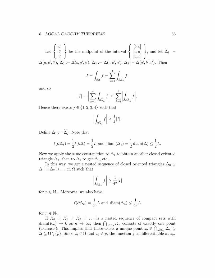
Let
a′
b′
c′
be the midpoint of the interval
[b, c][c, a][a, c]
, and let ∆1 :=
∆(a, c′, b′), ∆2 := ∆(b, a′, c′), ∆3 := ∆(c, b′, a′), ∆4 := ∆(a′, b′, c′). Then
I =
∫∂∆
f =4∑
k=1
∫∂∆k
f,
and so
|I| =
∣∣∣∣ 4∑k=1
∫∂∆k
f
∣∣∣∣≤ 4∑k=1
∣∣∣∣∫∂∆k
f
∣∣∣∣.Hence there exists j ∈ 1, 2, 3, 4 such that∣∣∣∣∫
∂∆j
f
∣∣∣∣ ≥ 1
4|I|.
Define ∆1 := ∆j. Note that
`(∂∆1) =1
2`(∂∆) =
1
2L and diam(∆1) =
1
2diam(∆) ≤ 1
2L.
Now we apply the same construction to ∆1 to obtain another closed orientedtriangle ∆2, then to ∆2 to get ∆3, etc.
In this way, we get a nested sequence of closed oriented triangles ∆0 ⊇∆1 ⊇ ∆2 ⊇ . . . in Ω such that∣∣∣∣∫
∂∆n
f
∣∣∣∣ ≥ 1
4n|I|
for n ∈ N0. Moreover, we also have
`(∂∆n) =1
2nL and diam(∆n) ≤ 1
2nL
for n ∈ N0.If K0 ⊇ K1 ⊇ K2 ⊇ . . . is a nested sequence of compact sets with
diam(Kn) → 0 as n → ∞, then⋂n∈N0
Kn consists of exactly one point(exercise!). This implies that there exists a unique point z0 ∈
⋂n∈N0
∆n ⊆∆ ⊆ Ω \ p. Since z0 ∈ Ω and z0 6= p, the function f is differentiable at z0.

6 LOCAL CAUCHY THEOREMS 57
Now let ε > 0 be arbitrary. Then there exists δ > 0 such that B(z0, δ) ⊆ Ωand ∣∣∣∣f(z)− f(z0)
z − z0
− f ′(z0)
∣∣∣∣ ≤ ε, (6)
whenever 0 < |z − z0| < δ. We can find n ∈ N such that
diam(∆n) ≤ 1
2nL < δ.
Then∆n ⊆ B(z0, L/2
n) ⊆ B(z0, δ) ⊆ Ω,
and so by (6) we have
|f(z)− f(z0)− f ′(z0)(z − z0)| ≤ ε|z − z0| (7)
whenever z ∈ ∆n.The functions z 7→ f(z0) and z 7→ f ′(z0)(z − z0) have the primitives
z 7→ zf(z0) and z 7→ 12f ′(z0)(z− z0)2, respectively. Hence by 4.7 (c) we have∫
∂∆n
f(z0) dz = 0 =
∫∂∆n
f ′(z0)(z − z0) dz.
It follows from (7) that∣∣∣∣∫∂∆n
f(z) dz
∣∣∣∣ =
∣∣∣∣∫∂∆n
(f(z)− f(z0)− f ′(z0)(z − z0)) dz
∣∣∣∣≤ `(∂∆n) sup
z∈∂∆n
|f(z)− f(z0)− f ′(z0)(z − z0)|
≤ 1
2nL supz∈∂∆n
ε|z − z0|
≤ ε1
2nL diam(∆) ≤ εL
1
2n· L 1
2n= εL2 1
4n.
This implies
|I| ≤ 4n∣∣∣∣∫∂∆n
f(z) dz
∣∣∣∣ ≤ 4nεL2 1
4n= εL2.
Since ε > 0 was arbitrary, we must have |I| = 0, and so I =
∫∂∆
f = 0 as
claimed.
6 LOCAL CAUCHY THEOREMS 58
2. We now assume that p coincides with one of the vertices a, b, c of ∆, sayp = a. Without loss of generality, the vertices a, b, c are distinct (otherwise,it is easy to see that the claim trivially holds). Then we may choose pointsb′ ∈ [a, b] and c′ ∈ [a, c] close to, but distinct from a = p.
Now let ∆1 = ∆(b′, b, c), ∆2 = ∆(c, c′, b′), and ∆3 = ∆(a, b′, c′). Then∫∂∆
f =
∫∂∆1
f +
∫∂∆2
f +
∫∂∆3
f.
Moreover, ∆1,∆2 ⊆ Ω \ p, and so∫∂∆1
f = 0 =
∫∂∆2
f
by the first part of the proof. Hence∫∂∆
f =
∫∂∆3
f,
and so ∣∣∣∣ ∫∂∆
f
∣∣∣∣ ≤ `(∂∆3) supz∈∂∆3
|f(z)|.
Since f is continuous at p, this function is bounded in a neighborhood of p.Choosing b′ and c′ close enough to p, we can make `(∂∆3) as small as wewant, while supz∈∂∆3
|f(z)| stays uniformly bounded. It follows that∣∣∣∣ ∫∂∆
f
∣∣∣∣ ≤ ε
for all ε > 0, which implies
∫∂∆
f = 0 as claimed.
3. Finally, we prove the claim if p ∈ ∆, but where p is not necessarilya vertex of ∆. We cut ∆ into three triangles so that p becomes a vertexin each of them; namely, we define ∆1 = ∆(a, b, p), ∆2 = ∆(b, c, p), and∆3 = ∆(c, a, p). Then∫
∂∆
f =
∫∂∆1
f +
∫∂∆2
f +
∫∂∆3
f,
and by the second part of the proof∫∂∆1
f =
∫∂∆2
f =
∫∂∆3
f = 0.

6 LOCAL CAUCHY THEOREMS 59
It follows that
∫∂∆
f = 0.
The proof is complete.
Corollary 6.4 (Cauchy’s Integral Theorem for convex sets). Suppose Ω ⊆ Cis an open convex set, p ∈ Ω, and f : Ω → C is a continuous function thatis holomorphic on Ω \ p. Then f has a primitive in Ω, i.e., there existsF ∈ H(Ω) such that F ′ = f .
In particular, ∫γ
f = 0,
whenever γ is a piecewise smooth loop in Ω.
Proof. Fix a ∈ Ω, and define
F (w) =
∫[a,w]
f(z) dz
for w ∈ Ω. Since Ω is convex, and so [a, w] ⊆ Ω, and since f is continuouson Ω, the function F is well defined.
Let w,w0 ∈ Ω be arbitrary. Then the triangle ∆ = ∆(a, w,w0) lies in Ω.So it follows from Goursat’s lemma that∫
∂∆
f =
∫[a,w]
f +
∫[w,w0]
f +
∫[w0,a]
f = 0.
Hence
F (w)− F (w0) =
∫[a,w]
f +
∫[w0,a]
f = −∫
[w,w0]
f =
∫[w0,w]
f.
So for w 6= w0 we get∣∣∣∣F (w)− F (w0)
w − w0
− f(w0)
∣∣∣∣ =∣∣∣∣ 1
w − w0
∫[w0,w]
f(z) dz − 1
w − w0
∫[w0,w]
f(w0) dz
∣∣∣∣=
1
|w − w0|
∣∣∣∣∫[w0,w]
(f(z)− f(w0)) dz
∣∣∣∣≤ sup
z∈[w0,w]
|f(z)− f(w0)| (by Lem. 4.9)
→0 as w → w0.
6 LOCAL CAUCHY THEOREMS 60
The last relation follows from the continuity of f at w0.So F is differentiable at w0, and F ′(w0) = f(w0). Since w0 was arbitrary,
we conclude that F ∈ H(Ω) and F ′ = f .The statement about path integrals now follows from 4.7 (c).
Lemma 6.5. Let a ∈ C, r > 0, γ(t) = a + reit for t ∈ [0, 2π], and z0 ∈B(a, r). Then ∫
γ
dz
z − z0
= 2πi.
Proof. It is not hard, but tedious to evaluate this integral by reducing it to in-tegrals over real-valued functions and applying a trigonometric substitution.We prefer to show the claim by using methods from complex analysis.
Note that for z ∈ C with |z − a| = r and z0 ∈ B(a, r) we have
1
z − z0
=1
(z − a)− (z0 − a)=
1
z − a· 1
1−(z0 − az − a
)=
1
z − z0
∞∑n=0
(z0 − az − a
)n=∞∑n=0
(z0 − a)n
(z − a)n+1.
This sum converges uniformly in z on the circle γ∗ = z ∈ C : |z − a| = r(to see this, use the Weierstrass M -test with
Mn :=1
r
(|z0 − a|
r︸ ︷︷ ︸< 1
)n
for n ∈ N0).Hence by Remark 5.15, we can integrate the infinite series term-by-term
and obtain ∫γ
dz
z − z0
=∞∑n=0
∫γ
(z0 − a)n
(z − a)n+1dz.
Now by Example 4.5 we have∫γ
dz
(z − a)n+1=
∫γ
(z − a)−n−1 dz =
2πi for n = 0,0 for n 6= 0.
Hence ∫γ
dz
z − z0
= 2πi · (z0 − a)0 = 2πi.

6 LOCAL CAUCHY THEOREMS 61
Corollary 6.6 (Cauchy’s Integral Formula. Version I). Let U ⊆ C be anopen set, a ∈ U , r > 0, f ∈ H(U), and γ(t) = a + reit for t ∈ [0, 2π]. IfB(a, r) ⊆ U , then
f(z0) =1
2πi
∫γ
f(z)
z − z0
dz
for all z0 ∈ B(a, r).
Proof. Suppose B(a, r) ⊆ U , and let z0 ∈ B(a, r). Note that γ∗ ⊆ U , and
z0 6∈ γ∗. So z 7→ f(z)− f(z0)
z − z0
is continuous on γ∗ and we can integrate this
function over γ∗.Since B(a, r) ⊆ U , and U is open, we can find a small number δ > 0 such
that for R := r + δ we have
B(a, r) ⊆ Ω := B(a,R) ⊆ U
(exercise!). Note that Ω is an open and convex set. Moreover, the functiong : Ω→ C defined by
g(z) =
f(z)− f(z0)
z − z0
for z ∈ Ω \ z0,
f ′(z0) for z = z0,
is continuous on Ω and holomorphic on Ω\z0. Since γ∗ ⊆ Ω, Corollary 6.4implies that∫
γ
f(z)
z − z0
dz − 2πif(z0) =∫γ
f(z)
z − z0
dz − f(z0)
∫γ
dz
z − z0
(by Lem. 6.5)
=
∫γ
f(z)− f(z0)
z − z0
dz
=
∫γ
g(z) dz = 0.
The statement follows.

7 Power series representations of holomor-
phic functions
Theorem 7.1. Let Ω ⊆ C be open, and f ∈ H(Ω). Then f has a localrepresentation as a power series at every point of Ω; more precisely, if z0 ∈ Ωis arbitrary, and r > 0 is such that B(z0, r) ⊆ Ω, then there exists a power
series∞∑n=0
an(z − z0)n that converges on B(z0, r) and satisfies
f(z) =∞∑n=0
an(z − z0)n
for all z ∈ B(z0, r).
Proof. Assume that B(z0, r) ⊆ Ω, fix z ∈ B(z0, r), and let γ(t) := z0 + reit
for t ∈ [0, 2π]. Then by Cauchy’s Integral Formula (Corollary 6.6) we have
f(z) =1
2πi
∫γ
f(w)
w − zdw.
Now for w ∈ ∂B(z0, r) we have
1
w − z=
1
(w − z0)− (z − z0)=
1
(w − z0)
1
1−(z − z0
w − z0
)=∞∑n=0
(z − z0)n
(w − z0)n+1.
Hencef(w)
w − z=∞∑n=0
(z − z0)n
(w − z0)n+1f(w) (8)
for all w ∈ ∂B(z0, r).The series in (8) (for fixed z) converges uniformly for w ∈ ∂B(z0, r) by
the Weierstrass M -test; indeed, since ∂B(z0, r) is a compact set and |f | iscontinuous on ∂B(z0, r), there exists K ≥ 0 such that
|f(w)| ≤ K for w ∈ ∂B(z0, r).
62

7 POWER SERIES REPRESENTATIONS 63
So for n ∈ N0 we have∣∣∣∣ (z − z0)n
(w − z0)n+1f(w)
∣∣∣∣ ≤ |z − z0|n
rn+1K =: Mn,
and
∞∑n=0
Mn =K
r
∞∑n=0
|z − z0|n
rn=K
r
1
1− |z − z0|r
=K
r − |z − z0|<∞.
Integrating the series in (8) term-by-term, we obtain
f(z) =1
2πi
∫γ
f(w)
w − zdw
=1
2πi
∫γ
( ∞∑n=0
(z − z0)n
(w − z0)n+1f(w)
)dw
=∞∑n=0
(1
2πi
∫γ
(z − z0)n
(w − z0)n+1f(w) dw
)=∞∑n=0
an(z − z0)n, (9)
where
an =1
2πi
∫γ
f(w)
(w − z0)n+1dw (10)
for n ∈ N0.Since an is independent of z, and z ∈ B(z0, r) was arbitrary, we see that
the series in (9) converges for all z ∈ B(z0, r) and represents f . The claimfollows.
Corollary 7.2. Let Ω ⊆ C be open, and f ∈ H(Ω). Then f ′ ∈ H(Ω).
This corollary establishes the fact used in Section 3.
Proof. By Theorem 7.1 the function f has a local power series representation;so f ′ can also be locally represented by a power series and f ′ ∈ H(Ω) asfollows from Theorem 5.9.
Corollary 7.3. Let Ω ⊆ C be open, and f ∈ H(Ω). Then f has derivativesf (n) of arbitrary order n ∈ N, and f (n) ∈ H(Ω).

7 POWER SERIES REPRESENTATIONS 64
Holomorphic functions are indefinitely differentiable!
Corollary 7.4. Let Ω ⊆ C be open, and f ∈ H(Ω). Then at each pointz0 ∈ Ω, the function f is represented by its Taylor series, and so
f(z) =∞∑n=0
f (n)(z0)
n!(z − z0)n.
This is valid for all z ∈ C with |z − z0| < dist(z, ∂Ω); in particular, if R isthe radius of convergence of the power series, then R ≥ dist(z0, ∂Ω).
In other words, the Taylor series of f converges and represents the func-tion in the largest open disk centered at z0 that is contained in Ω; if ∂Ω = ∅and so Ω = C, this means that this Taylor series converges and representsthe function for all z ∈ C.
Proof. By Theorem 7.1 the function f can locally be represented by a powerseries centered at z0. By Corollary 5.10 the coefficients of this power seriesare uniquely determined, because they are the Taylor coefficients of f at z0.Since each point z ∈ Ω with |z−z0| < dist(z0, ∂Ω) lies in a disk B(z0, r) withB(z0, r) ⊆ Ω, the claim follows from Theorem 7.1.
Corollary 7.5. Let Ω ⊆ C be open, and f ∈ H(Ω). Suppose that z0 ∈ Ω,r > 0, and B(z0, r) ⊆ Ω, and define γ(t) = z0 + reit for t ∈ [0, 2π]. Then
f (n)(z0) =n!
2πi
∫γ
f(z)
(z − z0)n+1dz (11)
for all n ∈ N0. Moreover, if |f(z)| ≤M for all z ∈ ∂B(z0, r), then for n ∈ N0
we have
|f (n)(z0)| ≤ n!M
rn(Cauchy estimates).
Proof. Equation (11) follows from formula (10) in the proof of Theorem 7.1,
since an =f (n)(z0)
n!is the n-th Taylor coefficient of f at z0.
Under the given assumptions, the Cauchy estimates follow from this:
|f (n)(z0)| =∣∣∣∣ n!
2πi
∫γ
f(z)
(z − z0)n+1dz
∣∣∣∣≤ n!
2π`(γ)
M
rn+1=n!
2π2πr
M
rn+1=n!M
rn.
7 POWER SERIES REPRESENTATIONS 65
Definition 7.6. A function f : C → C that is holomorphic on the wholecomplex plane C is called an entire function.
Corollary 7.7. Let f be an entire function. Then at each point z0 we canrepresent f by a power series
f(z) =∞∑n=0
an(z − z0)n
that converges for all z ∈ C.
Proof. This follows from Corollary 7.4.
Theorem 7.8 (Liouville’s Theorem). Every bounded entire function is con-stant.
Proof. Let f ∈ H(C) and suppose that there exists M ≥ 0 such that |f(z)| ≤M for all z ∈ C. Then f has a power series representation
f(z) =∞∑n=0
anzn
that converges for all z ∈ C. We know that
an =f (n)(0)
n!
for all n ∈ N0. The Cauchy estimates with z0 = 0 are valid for all n ∈ N0
and all r > 0. Hence
|an| =|f (n)(0)|
n!≤ M
rn
for all n ∈ N and all r > 0. Letting r → ∞ (for fixed n ∈ N), we see thatan = 0 for n ∈ N. So
f(z) =∞∑n=0
anzn = a0
for all z ∈ C. This shows that f is a constant function.
Theorem 7.9 (Fundamental Theorem of Algebra). Every non-constant com-plex polynomial has a root; more precisely, if n ∈ N, a0, a1, . . . , an ∈ C,an 6= 0, and P : C→ C,
P (z) = a0 + a1z + · · ·+ anzn (12)
for z ∈ C, then there exists z0 ∈ C such that P (z0) = 0.
7 POWER SERIES REPRESENTATIONS 66
Proof. Let P be a polynomial as in (12). We argue by contradiction andassume that P (z) 6= 0 for all z ∈ C. Then f = 1/P is an entire function.
Claim: f is bounded.Obviously, |P (z)| → ∞ as |z| → ∞. Hence there exists R > 0 such that
|P (z)| > |P (0)| whenever z ∈ C, |z| ≥ R,
and so|f(z)| < |f(0)| whenever z ∈ C, |z| ≥ R. (13)
Since f is continuous and B(0, R) is compact, there exists K ≥ 0 such that
|f(z)| ≤ K for all z ∈ B(0, R).
So|f(z)| ≤ maxK, |f(0)| for all z ∈ C.
The claim follows.Liouville’s Theorem now implies that f is constant. This is a contradic-
tion, since |f(R)| < |f(0)| by (13).
Corollary 7.10. The field C is algebraically closed.
Remark 7.11. If P 6= 0 is a polynomial as in (12), where an 6= 0, thenn ∈ N0 is called the degree of P , denoted by deg(P ). For the constantpolynomial P = 0 the degree is undefined.
If P and Q are polynomials and Q 6= 0, then we can divide P by Q withremainder by the usual division algorithm. Hence there exist polynomials Rand S such that
P = S ·Q+R,
where deg(R) < deg(Q) or R = 0.If z0 is a root of P 6= 0, then we can applies this to Q(z) := z − z0, and
we obtainP (z) = S(z)(z − z0) +R(z) for z ∈ C,
where deg(R) < deg(Q) = 1 or R = 0. So R must be a constant polynomial,and 0 = P (z0) = R(z0) shows that R = 0. We conclude that
P (z) = S(z)(z − z0) for z ∈ C.
7 POWER SERIES REPRESENTATIONS 67
If z0 is also a root of S, we can repeat this reasoning, etc. It follows thatthere exists k ∈ N and a polynomial T with T (z0) 6= 0 such that
P (z) = (z − z0)kT (z) for z ∈ C.
The number k is uniquely determined and called the multiplicity of the rootz0 of P .
Corollary 7.12. Every polynomial P of degree n ∈ N has precisely n rootscounting multiplicities; more precisely, if z1, . . . , zl ∈ C, l ∈ N, are thedistinct roots of P and k1, . . . , kl ∈ N their respective multiplicities, thenk1 + · · ·+ kl = n.
Moreover, there exists a ∈ C, a 6= 0, such that
P (z) = a(z − z1)k1 . . . (z − zm)km for z ∈ C.
Proof (Outline). This follows from induction on n. For the induction steplet P be a polynomial of degree n. Then P has a root z0 by the FundamentalTheorem of Algebra. Then P (z) = (z − z0)Q(z) for z ∈ C, where deg(Q) =n− 1. Now we apply the induction hypothesis to Q.
Theorem 7.13 (Morera’s Theorem). Let Ω ⊆ C be open, and f : Ω→ C becontinuous. Suppose that for every closed oriented triangle ∆ ⊆ Ω we have∫
∂∆
f = 0.
Then f is holomorphic on Ω.
This can be considered as a “converse” of Goursat’s lemma.
Proof. It is enough to show that f is holomorphic on every open disk B ⊆ Ω.If B is such a disk, fix a ∈ B and define
F (w) =
∫[a,w]
f(z) dz for w ∈ B.
This makes sense, since B is convex. As in the proof of Corollary 6.4, oneshows that F ∈ H(B) and F ′(w) = f(w) for w ∈ B. So in B the functionf is the derivative of a holomorphic function. Hence f is holomorphic itself(Corollary 7.2).

8 Zeros of holomorphic functions
Definition 8.1. Let (X, d) be a metric space, and A ⊆ X.
(a) A point x ∈ X is called an isolated point of A if x ∈ A and if thereexists ε > 0 such that B(x, ε) ∩ A = x.
(b) A point x ∈ X is called a limit point of A if for all ε > 0 the ball B(x, ε)contains infinitely many distinct points of A.
Remark 8.2. (a) A point x ∈ X is a limit point of A if and only if thereexists a sequence xn of distinct elements in A such that x = lim
n→∞xn.
(b) Every point x ∈ A is either an isolated point of A or a limit point ofA.
(c) A set K ⊆ X is compact if and only if every infinite set A ⊆ K has alimit point in K.
Theorem 8.3. Let Ω ⊆ C be a region, and f ∈ H(Ω). Define
Z(f) := a ∈ Ω : f(a) = 0 (the zero-set of f).
Then either Z(f) = Ω (iff f ≡ 0), or Z(f) is countable, consists of isolatedpoints, has no limit points in Ω.
In the latter case, for each a ∈ Z(f) there exists m ∈ N (the multiplicityor order of the zero a), and g ∈ H(Ω) with g(a) 6= 0 such that
f(z) = (z − a)mg(z) for z ∈ Ω. (14)
Proof. Let a ∈ Z(f), and fix r > 0 such that B(a, r) ⊆ Ω. By Corollary 7.4we can represent f by a power series
f(z) =∞∑n=0
an(z − a)n
for z ∈ B(a, r). Here a0 = f(a) = 0. Now either an = 0 for all n ∈ N, orthere exists a smallest m ∈ N such that am 6= 0.
In the first case, B(a, r) ⊆ Z(f). In the second case, we define
g(z) :=
1
(z − a)mf(z) for z ∈ Ω \ a,
∞∑n=0
an+m(z − a)n for z ∈ B(a, r).
68

8 ZEROS OF HOLOMORPHIC FUNCTIONS 69
The definitions for g agree in
(Ω \ a) ∩B(a, r) = B(a, r) \ a,
and show that g ∈ H(Ω). Moreover, g(a) = am 6= 0 and
f(z) = (z − a)mg(z) for z ∈ Ω. (15)
By continuity of g at a, there exists ε > 0 such that g(z) 6= 0 for z ∈B(a, ε) ⊆ Ω. Then (15) shows that f(z) 6= 0 for z ∈ B(a, ε) \ a, and so ais an isolated point of Z(f).
To summarize, either a whole neighborhood of a ∈ Z(f) belongs to Z(f)or a is an isolated point of Z(f).
Now let A be the set of limit points of Z(f) in Ω. We want to show thatA is open and relatively closed in Ω.
If a ∈ A, then there exists a sequence zn of distinct points in Z(f) suchthat a = lim
n→∞zn (Remark 8.2 (a)). By continuity of f we then have
f(a) = limn→∞
f(zn) = 0,
and so a ∈ Z(f). Then a is not an isolated point of Z(f), and so thereexists r > 0 such that B(a, r) ⊆ Z(f) by the first part of the proof. ThenB(a, r) ⊆ A which shows that A is an open set.
To establish that A is relatively closed in Ω we verify that Ω \A is open.To see this, let b ∈ Ω \ A be arbitrary. Then b is not a limit point of Z(f),and so by the first part of the proof there exists ε > 0 such that B(b, ε) ⊆ Ω,and B(b, ε) contains at most one point in Z(f). Then B(b, ε) ⊆ Ω \ A.
We have shown that A is open and relatively closed in Ω. Since Ω is aregion, we conclude that A = Ω or A = ∅. In the first case, Ω = A ⊆ Z(f) ⊆Ω, and so Z(f) = Ω.
In the second case, A = ∅ and so Z(f) has no limit points in Ω. By thefirst part of the proof, we also see that Z(f) consists of isolated points, andthat at each point a ∈ Z(f) the function f has a representation as in (15).
It remains to show that if Z(f) 6= Ω, then Z(f) is countable. The set Ω(as any open set in C) has a compact exhaustion; namely, there are compact
sets Kn ⊆ Ω for n ∈ N such that Kn ⊆ Kn+1 for n ∈ N, and⋃n∈N
Kn = Ω.
For example, we can take
Kn = z ∈ Ω : |z| ≤ n and dist(z, ∂Ω) ≥ 1/n.

8 ZEROS OF HOLOMORPHIC FUNCTIONS 70
Now Z(f) ∩Kn must be a finite set for each n ∈ N, for otherwise Z(f)would have a limit point in Kn (see Remark 8.2 (c)), and hence in Ω. So
Z(f) =⋃n∈N
(Kn ∩ Z(f))
is a countable union of finite sets, which implies that Z(f) is countable.
Example 8.4. (a) In Theorem 8.3 it is important that Ω is a region. Forexample, let Ω = B(0, 1) ∪B(1, 1) and
f(z) :=
0 for z ∈ B(0, 1),
ez for z ∈ B(1, 1),
Then f is holomorphic on Ω. We have Z(f) = B(0, 1) 6= Ω, but every pointin B(0, 1) is a limit point of Z(f) in Ω.
(b) Let f(z) = exp(1/z) − 1 for z ∈ Ω := C \ 0. Then f ∈ H(Ω), andZ(f) := 1/(2πin) : n ∈ Z \ 0. Then Z(f) 6= Ω has a limit point, namely0, but this point does not lie in Ω.
Theorem 8.5 (Uniqueness Theorem). Let Ω ⊆ C be a region, and f, g ∈H(Ω). If the set
z ∈ Ω : f(z) = g(z)has a limit point in Ω, then f = g.
Proof. Consider h = f − g ∈ H(Ω). Then the set
Z(h) = z ∈ Ω : h(z) = 0= z ∈ Ω : f(z) = g(z)
has a limit point in Ω. So Z(h) = Ω by Theorem 8.3 which implies h =f − g = 0. Hence f = g.
Theorem 8.6 (Maximum Modulus Theorem. Version I). Let Ω ⊆ C be aregion, and f ∈ H(Ω). If |f | attains a local maximum at a point in Ω, thenf is a constant function.
Proof. Suppose f attains a local maximum at a ∈ Ω. Then there exists ε > 0such that B(a, ε) ⊆ Ω and
|f(a)| ≥ |f(z)|

8 ZEROS OF HOLOMORPHIC FUNCTIONS 71
for all z ∈ B(a, ε). Replacing f by eiθf with suitable θ ∈ [0, 2π], we mayassume f(a) ≥ 0 without loss of generality. Then
f(a) = |f(a)| ≥ |f(z)| ≥ |Re(f(z))|
for z ∈ B(a, ε).Pick r ∈ (0, ε) and let γ(t) = a + reit, t ∈ [0, 2π]. Then by Cauchy’s
Integral Formula we have
f(a) =1
2πi
∫γ
f(z)
z − adz =
1
2πi
∫ 2π
0
f(a+ reit)
reitireit dt
=1
2π
∫ 2π
0
f(a+ reit) dt (Mean Value Property)
(the average of the function values on the circle γ is equal to the functionvalue at the center of the circle!). Hence
f(a) = Re(f(a)) =1
2π
∫ 2π
0
Re(f(a+ reit)
)dt
≤ 1
2π
∫ 2π
0
∣∣f(a+ reit)∣∣ dt
≤ 1
2π
∫ 2π
0
|f(a)| dt = |f(a)| = f(a).
So we must have equality in all these inequalities, which shows that∫ 2π
0
(∣∣f(a+ reit)∣∣− Re
(f(a+ reit)
))dt = 0,∫ 2π
0
(|f(a)| −
∣∣f(a+ reit)∣∣) dt = 0.
Since the integrands in these integrals are non-negative continuous functions,we conclude that
Re(f(a+ reit)
)=∣∣f(a+ reit)
∣∣ = |f(a)| = f(a)
for all t ∈ [0, 2π]. In particular,
Im(f(a+ reit)
)= 0,

8 ZEROS OF HOLOMORPHIC FUNCTIONS 72
and sof(a+ reit) = Re
(f(a+ reit)
)= f(a)
for all t ∈ [0, 2π]. This shows that the function f takes the constant valuef(a) on the circle ∂B(a, r). Hence f ≡ f(a) as follows from the UniquenessTheorem, and so f is a constant function.
We record two important facts that were derived in the proof of the lasttheorem.
Corollary 8.7. Let Ω ⊆ C be a region, f ∈ H(Ω), and a ∈ Ω and r > 0 besuch that B(a, r) ⊆ Ω. Then we have:
(a) f(a) =1
2π
∫ 2π
0
f(a+ reit) dt (Mean Value Property),
(b) |f(a)| ≤ max|f(a+ reit)| : t ∈ [0, 2π] with equality if and only if f isa constant function.
Proof. In the proof of Theorem 8.6 statement (a) was proved explicitly, andstatement (b) easily follows from the considerations in this proof.
Corollary 8.8. Let Ω ⊆ C be a region, f ∈ H(Ω), and a ∈ Ω and r > 0 besuch that B(a, r) ⊆ Ω. If f(z) 6= 0 for all z ∈ B(a, r), then we have
|f(a)| ≥ min|f(a+ reit)| : t ∈ [0, 2π] (16)
with equality if and only if f is a constant function.
Proof. If f has a zero on ∂B(a, r), then the inequality is obvious with strictinequality.
In the other case, where f has no zero on ∂B(a, r), we have f(z) 6= 0for all z ∈ B(a, r) by our hypotheses. Hence there exists R > r such that
B(a,R) ⊆ Ω and f is zero-free on Ω := B(a,R). For otherwise, we could finda sequence zn of zeros of f with |zn − a| → r. Passing to a subsequenceif necessary, we may without loss of generality assume that zn converges,say zn → w. Then
|w − a| = limn→∞
|zn − a| = r,
and so w ∈ ∂B(a, r) ⊆ Ω. Moreover, the continuity of f shows that
f(w) = limn→∞
f(zn) = 0.

8 ZEROS OF HOLOMORPHIC FUNCTIONS 73
This contradicts the fact that f has no zero on ∂B(a, r).
The function g := 1/f is then holomorphic on Ω, and so by Corol-lary 8.7 (b) we have
|g(a)| ≤ max|g(a+ reit)| : t ∈ [0, 2π]. (17)
By taking reciprocals here, we get (16). If we have equality in (16),
then we must have equality in (17). This implies that g is constant on Ω.
So f = 1/g is constant on Ω, and hence constant on Ω by the UniquenessTheorem.
Theorem 8.9 (Maximum Modulus Theorem. Version II). Let Ω ⊆ C be abounded region, and f : Ω→ C be a continuous function that is holomorphicon Ω. Then
max|f(z)| : z ∈ Ω = max|f(z)| : z ∈ ∂Ω (18)
The theorem says that the maximum of |f | on Ω (which exists by conti-nuity of |f | and compactness of Ω) is attained at some point on the boundary∂Ω of Ω. Note that ∂Ω 6= ∅, because the only open sets U ⊆ C with ∂U = ∅are U = C and U = ∅ (exercise!).
Proof. The maximum on the left-hand side of (18) is attained at some pointz0 ∈ Ω. If z0 ∈ ∂Ω, then (18) holds.
If z0 ∈ Ω, then f is constant on Ω by Theorem 8.6. Then f is alsoconstant on Ω by the continuity of f (exercise!). Since ∂Ω 6= ∅, again (18)holds.

9 The Open Mapping Theorem
Theorem 9.1. Let Ω ⊆ C be open, ϕ ∈ H(Ω), and z0 ∈ Ω. If ϕ′(z0) 6= 0,then ϕ is locally injective near z0 with a holomorphic inverse map.
More precisely, there exists an open neighborhood V ⊆ Ω of z0 such that
(i) ϕ is injective on V and ϕ′(z) 6= 0 for z ∈ V ,
(ii) W = ϕ(V ) is an open set,
(iii) the inverse map ψ := (ϕ|V )−1 is holomorphic on W .
Proof. Since ϕ ∈ H(Ω), we have ϕ′ ∈ H(Ω) by Corollary 7.2. In particular,ϕ′ is continuous at z0. Hence there exists δ > 0 such that B(z0, δ) ⊆ Ω and
|ϕ′(z)− ϕ′(z0)| ≤ 1
2|ϕ′(z0)| for all z ∈ B(z0, δ). (19)
Define V := B(z0, δ). Then V is an open convex neighborhood of z0.For z1, z2 ∈ V we have [z1, z2] ⊆ V , and so
|ϕ(z1)− ϕ(z2)| =∣∣∣∣∫
[z1,z2]
ϕ′(z) dz
∣∣∣∣=
∣∣∣∣∫[z1,z2]
ϕ′(z0) dz +
∫[z1,z2]
(ϕ′(z)− ϕ′(z0)) dz
∣∣∣∣≥∣∣∣∣∫
[z1,z2]
ϕ′(z0) dz
∣∣∣∣− ∣∣∣∣∫[z1,z2]
(ϕ′(z)− ϕ′(z0)) dz
∣∣∣∣ (20)
≥ |z1 − z2| · |ϕ′(z0)| − |z1 − z2| · maxz∈[z1,z2]
|ϕ′(z)− ϕ(z0)|
≥ 1
2|ϕ′(z0)| · |z1 − z2| by (19).
This inequality shows that ϕ is injective on V .Moreover, inequality (19) implies that
|ϕ′(z)| = |ϕ′(z0) + (ϕ′(z)− ϕ′(z0))|≥ |ϕ′(z0)| − |ϕ′(z)− ϕ′(z0)|
≥ 1
2|ϕ′(z0)|
74

9 THE OPEN MAPPING THEOREM 75
for z ∈ V . Hence ϕ′(z) 6= 0 for all z ∈ V . We have established (i).In order to prove (ii), let w ∈ W = ϕ(V ) be arbitrary. Then there exists
a ∈ V such that w = ϕ(a). Pick r > 0 such that B(a, r) ⊆ V . Then by (20)we have
|ϕ(a+ reit)− ϕ(a)| ≥ 1
2|ϕ′(z0)|r for t ∈ [0, 2π]. (21)
Let ε := 16|ϕ′(z0)|r > 0. We claim that B(w, ε) ⊆ W . Indeed, if u ∈ B(w, ε)
is arbitrary, then
|ϕ(a)− u| = |w − u| < ε ≤ 2ε− |ϕ(a)− u|< min
t∈[0,2π]|ϕ(a+ reit)− ϕ(a)| − |ϕ(a)− u| (by (21))
≤ mint∈[0,2π]
|ϕ(a+ reit)− u|.
By Corollary 8.8 this is only possible if ϕ − u has a zero in B(a, r). Hencethere exists z ∈ B(a, r) ⊆ V such that u = ϕ(z). This implies that u ∈ ϕ(V ),and so B(a, ε) ⊆ W . It follows that W is open.
To prove (iii) note that (20) can be rewritten as
|ψ(w1)− ψ(w2)| ≤ 2
|ϕ′(z0)|· |w1 − w2| for w1, w2 ∈ W .
This shows that ψ : W → V is continuous on W .In order to prove that ψ ∈ H(W ), let w ∈ W be arbitrary. Then there
exists a unique point z ∈ V with ϕ(z) = w. We claim that
ψ′(w) =1
ϕ′(z). (22)
Note that ϕ′(z) 6= 0 by (i). To prove (22), we have to show that if wn isan arbitrary sequence in W \ w with wn → w, then
limn→∞
ψ(wn)− ψ(w)
wn − w=
1
ϕ′(z).
If zn := ψ(wn) for n ∈ N, then zn → ψ(w) = z by the continuity of ψ.Therefore,
limn→∞
ψ(wn)− ψ(w)
wn − w= lim
n→∞
zn − zϕ(zn)− ϕ(z)
=1
ϕ′(z).
It follows that ψ ∈ H(W ). The proof is complete.
9 THE OPEN MAPPING THEOREM 76
Example 9.2. Let m ∈ N and πm : C → C be defined by πm(z) = zm forz ∈ C (the m-th power function). Then every point w = Reiβ 6= 0, R > 0,β ∈ R, has the m distinct preimages
zk = R1/meiβ/m+2πik/m, k ∈ 0, . . . ,m− 1.
This is also true for the point 0 if we count its only preimage 0 with mul-tiplicity m. So every point has exactly m preimages counting multiplicitiesand πm is “m-to-1”.
As the next theorem shows, a similar statement is true locally for everynon-constant holomorphic function.
Theorem 9.3. Let Ω ⊆ C be open, f ∈ H(Ω) be non-constant near z0 ∈ Ω,and w0 = f(z0). Let m ∈ N be the order of the zero of the function g := f−w0
at z0. Then there exists an open neighborhood V ⊆ Ω of z0, and ϕ ∈ H(V )such that
(i) g(z) = f(z)− w0 = ϕ(z)m for z ∈ V ,
(ii) ϕ is a bijective map from V onto a disk B(0, r) with r > 0, ϕ(z0) = 0,and ϕ′(z) 6= 0 for z ∈ V .
If we define U = B(w0, rm), ψ(w) = w − w0, and let πm be the m-th
power function as in Example 9.2, then we get a commutative diagram
Vf
//
ϕ
U
ψ
B(0, r)πm // B(0, rm).
Here the maps ϕ and ψ can be considered as bijective holomorphic “changesof coordinates”. So near z0 the map f behaves in the same way as πm and islocally m-to-1.
Proof. Without loss of generality, Ω is a convex open neighborhood of z0 suchthat f(z)− w0 6= 0 for z ∈ Ω \ z0 (this is based on Theorem 8.3). Then
f(z)− w0 = (z − z0)m · h(z) for z ∈ Ω,
where h ∈ H(Ω) and h(z) 6= 0 for all z ∈ Ω (see Theorem 8.3).

9 THE OPEN MAPPING THEOREM 77
We have h′/h ∈ H(Ω), and so h′/h has a primitive k ∈ H(Ω) by Corol-lary 6.4 which means k′ = h′/h.
Then(he−k)′ = h′e−k − hk′e−k = h′e−k − h′e−k = 0,
and so he−k is a constant function. Then he−k ≡ h(z0)e−k(z0) 6= 0. Thereexists c ∈ C such that ec = h(z0)e−k(z0) = he−k. Define l := k + c. Thenl ∈ H(Ω) and
el = ekec = ekhe−k = h.
Define ϕ(z) := (z−z0)el(z)/m for z ∈ Ω. Then ϕ ∈ H(Ω) and g = f−w0 = ϕm.Moreover, ϕ(z0) = 0 and ϕ′(z0) = el(z0)/m 6= 0. By Theorem 9.1 we can
choose an open neighborhood V of z0 such that ϕ|V is a bijection onto some
open neighborhood W of ϕ(z0) = 0 and such that ϕ′(z) 6= 0 for z ∈ V . Nowpick r > 0 such that B(0, r) ⊆ W and let V := ϕ−1(B(0, r)). Then V and ϕ(restricted to V ) have the desired properties.
Remark 9.4. The number m in Theorem 9.3 is called the local degree of fat z0, written m = degf (z0). Note that
f ′(z0) = mϕ′(z0) · ϕ(z0)m−1
6= 0 for m = 1,
= 0 for m ≥ 2.
So m = degf (z0) ≥ 2 if and only if f ′(z0) = 0.The zeros of f ′ are called the critical points of f . Each image point of
a critical value is called a critical value of f . The critical points of f areprecisely the points where the local degree is greater than 1. If f is a non-constant holomorphic function on a region Ω, then the set of critical pointsof f consists of isolated points and has no limit point in Ω as follows fromthe Uniqueness Theorem.
Corollary 9.5 (Open Mapping Theorem). Let Ω ⊆ C be a region, andf ∈ H(Ω) be non-constant. Then f is an open map, i.e., the image f(U)of every open set U ⊆ Ω is open. Moreover, the image f(U) of every regionU ⊆ Ω is a region.
Proof. The first part follows from Theorem 9.3. So if U ⊆ Ω is a region, thenf(U) is open. Moreover, f(U) is also connected as the continuous image ofa connected set. Hence f(U) is a region.
9 THE OPEN MAPPING THEOREM 78
Corollary 9.6. Let Ω ⊆ C be a region, and f : Ω → C be a holomorphicfunction that is a bijection onto its image Ω := f(Ω) (i.e., f : Ω → Ω is a
bijection). Then f ′(z) 6= 0 for all z ∈ Ω, the inverse map g := f−1 : Ω → Ω
is holomorphic on the open set Ω, and we have
g′(w) =1
f ′(g(w))for all w ∈ Ω. (23)
Proof. Since f is a bijection, the local degree of f must be equal to 1 at eachpoint of Ω. Hence f ′(z) 6= 0 for all z ∈ Ω by Remark 9.4. By Corollary 9.5
the set Ω is open, and g = f−1 is holomorphic on Ω by Theorem 9.1 (iii).
Since f(g(w)) = w for all w ∈ Ω, we conclude from the chain rule that
f ′(g(w)) · g′(w) = 1
for w ∈ Ω. So (23) follows.

10 Elementary functions
10.1. Trigonometric functions. How can we define sin z and cos z forz ∈ C so that
(i) the definitions agree with the usual definition for z ∈ R,
(ii) sin and cos are holomorphic on C?
By the Uniqueness Theorem this is possible in at most one way, and byCorollary 7.7 the functions sin and cos should have power series representa-tions converging on C.
So we define
sin z =∞∑n=0
(−1)nz2n+1
(2n+ 1)!and cos z =
∞∑n=0
(−1)nz2n
(2n)!
for z ∈ C. These series converge for all z ∈ C by the ratio test; so byTheorem 5.9 the functions sin and cos are holomorphic on C. Moreover,with these definitions we get the usual functions for z ∈ R by the well-knownpower series representations for sin and cos on R.
All the standard trigonometric identities are also valid for complex argu-ments. For example, we have
sin2 z + cos2 z = 1 for z ∈ C.
Indeed, the functions on both sides of this equation are holomorphic functionsof z on C. They are the same for z ∈ R. So by the Uniqueness Theoremthey are the same for all z ∈ C.
Similarly, we have
sin(z + w) = sin z cosw + cos z sinw (24)
for z, w ∈ C.Indeed, we know that (24) holds for z, w ∈ R. Fix w ∈ R. Then
z 7→ sin(z + w) and z 7→ sin z cosw + cos z sinw
are holomorphic functions on C that are identical on R. So they have thesame values for all z ∈ C. We conclude that (24) holds for all z ∈ C, w ∈ R.
79

10 ELEMENTARY FUNCTIONS 80
Now fix z ∈ C and consider the right-hand and the left-hand side of (24)as holomorphc functions of w on C. They agree for w ∈ R, and so they agreefor all w ∈ C by the uniqueness theorem. So (24) holds for all z, w ∈ C.
We have
sin z =eiz − e−iz
2iand cos z =
eiz + e−iz
2for z ∈ C. (25)
Again we note that both sides in these equations are holomorphic functionsof z on C, and that the function agree for z ∈ R. For example, for z = t ∈ Rwe have
eit − e−it
2i=
(cos t+ i sin t)− (cos t− i sin t)
2i= sin t.
So the equations (25) are valid for all z ∈ C.An immediate consequence of (25) is the identity
eiz = cos z + i sin z for z ∈ C (Euler’s formula).
What are the zeros of the functions sin and cos? Note that
sin z = 0 ⇔ eiz − e−iz = 0
⇔ e2iz = 1
⇔ 2iz = 2πik for some k ∈ Z⇔ z = πk for some k ∈ Z.
Since cos z = sin(π2− z) for z ∈ C, we have
cos z = 0 ⇔ z =π
2+ kπ for some k ∈ Z.
We can compute sin z and cos z for z = x + iy, x, y ∈ R, by using theaddition formulas. First note that
cos(iy) =e−y + ey
2= cosh y, sin(iy) =
e−y − ey
2i= i sinh y.
Hence
cos(x+ iy) = cos x cos(iy)− sinx sin(iy)
= cosx cosh y − i sinx sinh y,

10 ELEMENTARY FUNCTIONS 81
and similarlysin(x+ iy) = sinx cosh y + i cosx sinh y.
The functions tan and cot are defined in the usual way. So
tan z :=sin z
cos z
is a holomorphic function of z on C \ kπ + π/2 : k ∈ Z and
cot z :=cos z
sin z
is a holomorphic function of z on C \ kπ : k ∈ Z.
10.2. Logarithms. Every solution of the equation z = ew is called a log-arithm of z. A number z ∈ C has a logarithm if and only if z 6= 0. Letz = reiα, r > 0, α ∈ R. Then
z = elog r+iα = ew
iff w = log r + iα + 2πik, k ∈ Z. So every z ∈ C \ 0 has infinitely manylogarithms.
A continuous function L : Ω → C defined on a region Ω ⊆ C is called abranch of the logarithm if eL(z) = z for all z ∈ Ω. Note that 0 6∈ Ω if a branchof the logarithm exists, but this condition is not sufficient for the existenceof the branch of the logarithm on a region Ω. For example, if Ω = C \ 0,then no branch of the logarithm exists on Ω.
If L1, L2 : Ω→ C are two branches of the logarithm, then eL1(z) = eL2(z),and so eL1(z)−L2(z) = 1 for all z ∈ Ω. It follows that
(L1 − L2)(Ω) ⊆ 2πik : k ∈ Z.
Since (L1 − L2)(Ω) is a connected set, we conclude that there exists k ∈ Zsuch that
L1(z) = L2(z) + 2πik
for all z ∈ Ω. So the branches of the logarithm in a region are obtained fromone branch (if it exists) by adding 2πik, k ∈ Z. In particular, knowing thefunction value of a branch at one point determines the branch uniquely.
The exponential function maps the strip
S := w ∈ C : −π < Im(w) < π
10 ELEMENTARY FUNCTIONS 82
bijectively onto the slit plane C \ (−∞, 0]. By Corollary 9.6 the functionexp |S has a holomorphic inverse function denoted by log and called theprincipal branch of the logarithm. It is the unique branch of the logarithmon Ω = C \ (−∞, 0] with log 1 = 0.
By Corollary 9.6 we have
d
dzlog z =
1
elog z=
1
z.
The expression log z agrees with the usual definition for z > 0. Note that logis discontinuous along the “branch cut” (−∞, 0]. Indeed, if for fixed r > 0the points z1 = reiα1 and z1 = reiα2 with α1, α2 ∈ (−π, π) approach −r fromthe upper and lower half-planes, respectively, then α1 → π and α2 → −π.So
log(z1) = log r + iα1 → log r + iπ
andlog(z2) = log r + iα2 → log r − iπ.
This shows that the values of the principal branch of the logarithm differ by2πi on “different sides” of the branch cut.
Note that in general we have
log(z1z2) 6= log(z1) + log(z2)
if log is the principal branch of the logarithm. For example, if z1 = z2 = i ∈C \ (−∞, 0], then z1z2 = i2 = −1 is not even contained in the domain ofdefinition C \ (−∞, 0] of the principal branch.
10.3. Roots and powers. If Ω ⊆ C is a region where a branch L of thelogarithm exists, we define for a ∈ C and z ∈ Ω,
za := exp(aL(z)).
Note that if L is another branch of the logarithm, then L = L+ 2πik, k ∈ Z,and so
exp(aL(z)) = exp(aL(z) + a2πik) = exp(aL(z)) exp(a2πik)
for z ∈ Ω. So different branches of the power function za differ by a multi-plicative factor. If a ∈ Z, then exp(a2πik) = 1, and so there exists only onebranch. So for a = n ∈ Z, z 6= 0,
za = exp(aL(z)) =(
exp(L(z))a
= zn

10 ELEMENTARY FUNCTIONS 83
agrees with the power function as defined in Section 1.Unless otherwise stated, za will denote the principal branch defined on
C \ (−∞, 0] asza := exp(a log(z)),
where log is the principal branch of the logarithm. This branch is normalizedso that
1a = exp(a log(0)) = exp(0) = 1,
and agrees with the usual definition of the power function for z > 0, a ∈ R.Note that
d
dzza =
d
dzexp(a log(z)) = a
1
zexp(a log(z))
= a exp(− log(z)) exp(a log(z)) = a exp((a− 1) log(z)) = aza−1
for z ∈ C \ (−∞, 0].If z = reiα, r > 0, α ∈ (−π, π), we have
za = exp(a log(reiα)) = exp(a(log r + iα)).
For a > 0 this means that
za = exp(a(log r + iα)) = raeiαa.
In particular, a sector
S = reiα : R > 0, ϕ1 < α < ϕ2,
where −π ≤ ϕ1 < ϕ2 ≤ π and whose opening angle ϕ2 − ϕ1 is sufficentlysmall, is mapped by z 7→ za onto the sector
S ′ = ρeiβ : ρ > 0, aϕ1 < α < aϕ2
whose opening angle differs from the opening angle of S by the factor a.If a = 1/n, where n ∈ N, we also use the notation
n√z := z1/n = za.
For the principal branch we get
n√reiα = r1/neiα/n
10 ELEMENTARY FUNCTIONS 84
for z = reiα, r > 0, α ∈ (−π, π).Note that if r > 0 is fixed and z1 = reiα approaches the point −r on the
branch cut (−∞, 0] from the upper half-plane, then α → π and so n√z1 =
n√reiα → r1/neiπn. Similarly, if z2 = reiα approaches the point −r on the
branch cut from the lower half-plane, then α→ −π and so n√z2 =
n√reiα →
r1/neiπn → r1/ne−iπn.In particular, if n = 2, then the values of
√z for z = −r on “different
sides of the branch cut” are√ri and −
√ri. So these values differ by a factor
−1.
10.4. Riemann surfaces spread over the plane. How can we get rid ofthe artificial branch cut of the logarithm? We cannot define the logarithmas a “sensible” (for example, continuous) function on C \ 0. Indeed, eachz = reiα ∈ C \ 0 as infinitely many logarithms
log r + iα + 2πik, k ∈ Z, (26)
and these values cannot be patched up to a continuous function on C \0. So the logarithm is a “multi-valued” function. To get a well-definedfunction in the usual sense, one introduces a surface with infinitely manylayers (roughly speaking, one layer for each k ∈ Z in (26)) so that on thissurface the logarithm is a well-defined and continuous function.
One way to do this is as follows. Let S = (z, w) ∈ C2 : z = exp(w).Then we may think of S as a “covering surface” of C \ 0 where each point(z, w) ∈ S lies “above” the point z. The logarithm is then defined as themap (z, w) ∈ S 7→ w.
Another way to visualize this Riemann surface spread over C \ 0 is bythe following gluing procedure. For k ∈ Z let
Pk = reiα : r > 0, 2πi(k − 1) ≤ α ≤ 2πi(k + 1)be a copy of punctured complex plane, where the points in Pk with α =2πi(k ± 1) on different sides of the branch cut (−∞, 0] are considered asdistinct. Then the Riemann surface S of the logarithm is obtained by gluingtogether (i.e., identifying) each point rei2πi(k+1), r > 0, on the upper side ofthe branch cut of Pk with the same point on lower side of the branch cut ofPk+1. On a more intuitive level, this surface has the shape of a “bi-infinitespiral staircase” lying above C \ 0.
The logarithm on this surface S is defined as follows. If z ∈ S, thenz ∈ reiα ∈ Pk for some k ∈ Z, where 2πi(k − 1) ≤ α ≤ 2πi(k + 1). Then weset log(z) := log r + iα. This is a well-defined function on S.

10 ELEMENTARY FUNCTIONS 85
10.5. The Riemann surface of√z. The square-root function has two
branches on C \ (−∞, 0] that differ by the factor ±1. To get a well-definedsquare-root function we define a Riemann surface S = (z, w) ∈ C2 : z =w2. Then by the projection map (z, w) ∈ S 7→ z this surface is spread overthe complex plane C. On S the square-root function is given by the map(z, w) ∈ S 7→ w.
Similarly as for the logarithm, one can obtain S from a gluing procedurealso as follows. We take two copies P+ and P− of the complex plane with a slitalong the negative real axis (−∞, 0] as branch cut. In each copy we considerthe points re±iπ, r > 0, on different sides of the branch cut as distinct. Thenwe glue P+ and P− together “cross-wise” so that the point re+iπ ∈ P+ isidentified with re−iπ ∈ P−, and re−iπ ∈ P+ is identified with re+iπ ∈ P−. Wealso identify 0 ∈ P+ with 0 ∈ P−. Each point z ∈ S can be considered aslying above its corresponding point z ∈ P+ or z ∈ P− considered as a pointin the complex plane. In this way, S is a Riemann surface spread over Cwith a natural projection map S → C that is locally injective away from theso-called branch point 0 ∈ S.
The surface S cannot be realized as an embedded surface in R3, but ifone wants a model of S in R3 one has to allow a “self-intersection” of S alongthe branch cut.
If z ∈ S is arbitrary, then the point z lies in one of the copies P+ or P−(or both). If z ∈ P+ or z ∈ P− and z = reiα, where r ≥ 0 and −π ≤ α ≤ π,we define
√z =√reiα/2 or
√z = −
√reiα/2, respectively. This gives a well-
defined square-root function on S.
11 The Riemann sphere
11.1. The extended complex plane. We want to compactify C by addinga point at infinity denoted by ∞. Then C := C∪ ∞ is called the extended
complex plane. One can visualize C as the Riemann sphere by stereographicprojection.
To do this, let S = (u, v, w) ∈ R3 : u2 + v2 +w2 = 1 be the unit spherein R3. We consider the complex plane as a subset of R3 by the identificationz = x + iy ∈ C ∼= (x, y, 0) ∈ R3, where x, y ∈ R. Then the sphere S cutsC along its equator. Let N = (0, 0, 1) be the “north pole” of S. Thenone defines a projection map π : S \ N → C as follows. If Z ∈ S \ Nis arbitrary, then we join N and Z by a line L. The line L intersects thecomplex plane C ⊆ R3 in a unique point z. We define π(Z) := z. Thisstereographic projection π gives a bijection of S \ N onto C.
It is easy to find an explicit formula for the map π and its inverse. IfZ = (x1, x2, x3) ∈ S \ N is arbitrary, then the line L passing through Zand N is given by
L = t(x1, x2, x3) + (1− t)(0, 0, 1) ∈ R3 : t ∈ R.
The line L meets C at a point z determined by the equation
tx3 + (1− t) = 0.
Hence t = 1/(1−x3). Inserting this back into the parametrization of L gives
Z = (x1, x2, x3) ∈ S \ N 7→ π(Z) = z =x1 + ix2
1− x3
∈ C.
Conversely, let z = x + iy ∈ C be arbitrary, where x, y ∈ R. The line L′
passing through N = (0, 0, 1) and (x, y, 0) ∼= z is given by
L′ = t(x, y, 0) + (1− t)(0, 0, 1) ∈ R3 : t ∈ R.
A point on L′ different from N lies on S iff
t2x2 + t2y2 + (1− t)2 = t2|z|2 + (1− t)2 = 1
⇒ t2(|z|2 + 1) = 2t
⇒ t =2
|z|2 + 1(t = 0 corresponds to N).
86
11 THE RIEMANN SPHERE 87
Hence
z = x+ iy ∈ C 7→ π−1(z) =
(2x
|z|2 + 1,
2x
|z|2 + 1,|z|2 − 1
|z|2 + 1
)∈ S \ N.
If we make |z| larger and larger, then the corresponding point Z = π−1(z)on S gets closer and closer to N . So it is natural to extend π to a bijectionfrom S onto C by setting π(N) =∞. In this way, we can identify C with S
by stereographic projection and refers to C as the Riemann sphere.Let z, w ∈ C be points in the complex plane, and Z = π−1(z) and W =
π−1(w). Then for the Euclidean distance of Z and W we get
|Z −W |2 =
∣∣∣∣ 2z
|z|2 + 1− 2w
|w|2 + 1
∣∣∣∣2 +
(|z|2 − 1
|z|2 + 1− |w|
2 − 1
|w|2 + 1
)2
=4|z(|w|2 + 1)− w(|z|2 + 1)|2 + 4(|z|2 − |w|2)2
(|z|2 + 1)2(|w|2 + 1)2
= −4zw + wz
(|z|2 + 1)(|w|2 + 1)+ 4|z|2(|w|2 + 1)2 + |w|2(|z|2 + 1)2 + (|z|2 − |w|2)2
(|z|2 + 1)2(|w|2 + 1)2
= −4zw + wz
(|z|2 + 1)(|w|2 + 1)+ 4
(|z|2 + |w|2)(|z|2 + 1)(|w|2 + 1)
(|z|2 + 1)2(|w|2 + 1)2
= 4|z|2 + |w|2 − zw − wz
(|z|2 + 1)(|w|2 + 1)= 4
|z − w|2
(|z|2 + 1)(|w|2 + 1),
and so
|Z −W | = 2|z − w|√1 + |z|2
√1 + |w|2
.
Moreover,
|Z −N |2 =4|z|2
(|z|2 + 1)2+
4
(|z|2 + 1)2=
4
(|z|2 + 1),
and so
|Z −N | = 2√1 + |z|2
.
11.2. The chordal metric. We define a distance function on C = C∪∞as follows. For z, w ∈ C ⊆ C we define
d(z, w) :=2|z − w|√
1 + |z|2√
1 + |w|2,

11 THE RIEMANN SPHERE 88
d(z,∞) = d(∞, z) :=2√
1 + |z|2,
and let d(∞,∞) = 0.As we have seen above, d corresponds to the Euclidean metric on S by
stereographic projection. This shows that d is a metric on C, called thechordal metric. Unless otherwise stated, C will always carry this metric.
Stereographic projection is an isometry between S equipped with the (re-
striction of the) Euclidean metric on R3 and C equipped with the chordal
metric. In particular, S and C are homeomorphic (i.e., there exists a contin-uous bijection between these spaces with continuous inverse). So the topo-
logical and metric properties of S and C are the same. In particular, C is acompact metric space.
Remark 11.3. It is not hard to show that C equipped with the restriction ofthe chordal metric and C equipped with the usual Euclidean metric have thesame topology (i.e., the same open sets). So chordal and Euclidean metricsare equivalent metrics.
In particular, if zn is a sequence in C and z ∈ C, then zn → z withrespect to the chordal metric if and only if zn → z with respect to theEuclidean metric.
We have zn →∞ ∈ C (convergence in the metric space C) iff
d(zn,∞) =2√
1 + |zn|2→ 0
iff |zn| → +∞ (in the sense of real analysis).
Definition 11.4. Let X be a topological Hausdorff space (e.g., a metricspace), and n ∈ N. Then X is called a (topological) n-manifold if every pointx ∈ X has an open neighborhood that is homeomorphic to an open subsetof Rn.
A chart on an n-manifold X is a homeomorphism ϕ : U → V of an opensubset U ⊆ X onto an open subset V ⊆ Rn. An atlas on X is a familyA = ϕi : Ui → Vi : i ∈ I of charts on X such that X =
⋃i∈I Ui, i.e., the
chart neighborhoods of charts in the family cover the whole manifold X.
Recall that a topological space X is called Hausdorff if for all pointsx, y ∈ X, x 6= y, there exists open sets U, V ⊆ X with x ∈ U , y ∈ V , andU ∩ V = ∅.
11 THE RIEMANN SPHERE 89
Our definition of an n-manifold is slightly non-standard as one usuallyrequires that an n-manifold should have a countable basis for its topology(i.e., there exists a countable set B of open sets in X such that every openset in U is a union of sets in B).
We are mostly interested in the case n = 2. A 2-manifold is also called asurface. If we make the identification R2 ∼= C, then we can think of a charton a surface as a map into C.
Example 11.5. The unit sphere S ⊆ R3 (and hence also C) is a topological2-manifold. To see this, it is enough to exhibit an atlas of charts on S. It con-sists of two charts, namely the map ϕ1 : S \n → R2 given by stereographicprojection from the north pole n = (0, 0, 1), and the map ϕ2 : S \ s → R2
given by stereographic projection from the south pole s = (0, 0,−1) (definedin the obvious way).
Similarly, one can define an atlas on C given by two charts ψ1 and ψ2. Hereψ1 : U1 := C ⊆ C→ C, ψ1(z) = z for z ∈ C, and ψ2 : U2 := C \ 0 ∪ ∞ ⊆C→ C,
ψ2(z) =
1/z for z ∈ C \ 0,
0 for z =∞.
Definition 11.6. Let U, V ⊆ C be open sets. A map f : U → V is calleda biholomorhism if f is a bijection, f is holomorphic on U , and f−1 is holo-morphic on V .
Two charts ϕ1 : U1 → V1 ⊆ C and ϕ2 : U2 → V2 on a 2-manifold X arecalled holomorphically compatible if U1 ∩ U2 = ∅, or if U1 ∩ U2 6= ∅ and themap
ϕ2 ϕ−11 |ϕ1(U1 ∩ U2) : ϕ1(U1 ∩ U2)→ ϕ2(U1 ∩ U2)
is a biholomorphism.
Example 11.7. Let ψ1 : U1 → C and ψ2 : U2 → C be the charts on C asin Example 11.5. Then ψ1 and ψ2 are holomorphically compatible. Indeed,U1 = C and U2 = C \ 0 ∪ ∞, and so U1 ∩ U2 = C \ 0. Then W :=ψ1(U1 ∩ U2) = ψ2(U1 ∩ U2) = C \ 0. Moreover, f := ψ2 ψ−1
1 |W : W → Wis given by f(z) = 1/z for z ∈ W . This is a holomorphic bijection withholomorphic inverse z 7→ f−1(z) = 1/z.
Definition 11.8. An atlas A = ϕi : Ui → Vi ⊆ C : i ∈ I on a 2-manifoldX is called a complex atlas if the charts in A are pairwise holomorphicallycompatible.

11 THE RIEMANN SPHERE 90
Two complex atlases A1 and A2 on X are called analytically equivalent ifeach chart in A1 is holomorphically compatible with each chart in A2. Thisdefines an equivalence relation for atlases. A complex structure on X is anequivalence class of analytically equivalent atlases on X. A Riemann surfaceis a topological 2-manifold equipped with a complex structure.
Remark 11.9. One should think of the complex structure on a Riemannsurface as being represented by some fixed complex atlas. A complex charton a Riemann surface is a chart that is holomorphically compatible with allthe charts in one atlas (and hence in all atlases) that define the complexstructure. Often it is convenient to add complex charts to a given atlas asneeded, for example if one wants to make the chart neighborhoods smaller:if ϕ : U → V is a chart in a complex atlas A, and U ′ ⊆ U is open, thenϕ|U ′ : U ′ → ϕ(U ′) is a chart that is holomorphically compatible with eachchart in A.
Definition 11.10. Let X be a Riemann surface, and f : X → C. Then f iscalled a holomorphic function if for every complex chart ϕ : U → V ⊆ C onX the function f ϕ−1 : V → C is a holomorphic function on the open setV ⊆ C.
Definition 11.11. Let X and Y be Riemann surfaces, and f : X → Ybe continuous. Then f is called a holomorphic map (between X and Y ) iffor every complex chart ϕ : U → V ⊆ C on X and every complex chartψ : U ′ → V ′ ⊆ C on Y with f(U) ⊆ U ′ the function ψ f ϕ−1 : V → V ′ isholomorphic.
Note that the function ψ f ϕ−1 is defined on the open set V ⊆ C andtakes values in V ′ ⊆ C. So it makes sense to require the holomorphicity ofthis function (as defined in Section 3).
Example 11.12. The atlas A consisting of the charts ψ1 and ψ2 on theRiemann sphere C as defined Example 11.5 is a complex atlas (see Exam-
ple 11.7). In the following, we always think of C as a Riemann surfaceequipped with the complex structure represented by the complex atlas A.
How do we verify that a given continuous map f : C→ C is holomorphic?We check this locally near each point z0 ∈ C. Let w0 := f(z0). The basicidea is this: whenever the point ∞ is involved, we send it to 0 by the chartψ2. This leads to several cases.

11 THE RIEMANN SPHERE 91
Case 1: z0, w0 ∈ C. In this case, z 7→ f(z) is just a complex-valuedfunction near z0, and we check its holomorphicity as usual.
Case 2: z0 =∞, w0 ∈ C. We check z 7→ g(z) := f(1/z) for holomorphic-ity near 0.
Here it is understood that g(0) := f(∞), and we make similar definitionsin the remaining two cases.
Case 3: z0 ∈ C, w0 = ∞. We check z 7→ 1/f(z) for holomorphicity nearz0 ∈ C.
Case 4: z0 = w0 = ∞. We check z 7→ 1/f(1/z) for holomorphicity near0.
Example 11.13. Every rational function R can be considered as a holo-morphic map R : C → C. To see this, let R = P/Q, where P and Q arepolynomials with no common roots and Q 6= 0. We write
P (z) = a0 + a1z + · · ·+ anzn, an 6= 0,
Q(z) = b0 + b1z + · · ·+ bkzk, bk 6= 0.
Then R is given by R(z) = P (z)/Q(z) for z ∈ C if Q(z) 6= 0. We extend R
continuously to a map R : C→ C. To do this, we set
R(z) := limw→z
R(w) =∞
for z ∈ C if Q(z) = 0 (note that then P (z) 6= 0) and
R(∞) := limw→∞
R(w) =
0 if n < k,
an/bk if n = k,∞ if n > k.
Then R(z) is defined for all z ∈ C, and R : C→ C is continuous.
Moreover, R : C → C is a holomorphic map as can be seen by the caseanalysis as in Example 11.12.
For example, suppose z0 ∈ C and Q(z0) = 0. Then R(z0) = ∞, and sowe have to investigate the holomorphicity of
z 7→ 1
R(z)=Q(z)
P (z)(27)
near z0. Since P and Q have no common roots, we have P (z0) 6= 0 and soP (z) 6= 0 for z near z0. The holomorphicity of the function in (27) near z0
follows.

12 Mobius transformations
Definition 12.1. A rational map R : C→ C of the form
R(z) =az + b
cz + dwith a, b, c, d ∈ C, ad− bc 6= 0, (28)
is called a Mobius transformation. The set of all Mobius transformations isdenoted by Mob.
The condition ad − bc 6= 0 in (28) ensures that we cannot cancel thenumerator against denominator in the formula for R(z). Note that ad − bc
is the determinant of the coefficient matrix
(a bc d
)associated with R.
12.2. Composition of Mobius transformations. The composition of twoMobius transformations is again a Mobius transformation. This operationcorresponds to multiplication of the associated coefficient matrices. Indeed,suppose that S, T ∈ Mob, where
S(w) =a11w + a12
a21w + a22
, and w = T (z) =b11z + b12
b21z + b22
.
Let
A =
(a11 a12
a21 a22
)and B =
(b11 b12
b21 b22
)be the corresponding coefficient matrices. Then S T is also a Mobius trans-formation, because
(S T )(z) = S(T (z)) =a11
b11z + b12
b21z + b22
+ a12
a21b11z + b12
b21z + b22
+ a22
=(a11b11 + a12b21)z + a11b12 + a12b22
(a21b11 + a22b21)z + a21b12 + a22b22
,
and its associated coefficient matrix is(a11b11 + a12b21 a11b12 + a12b22
a21b11 + a22b21 a21b12 + a22b22
)= AB,
which is the product of A and B.
92
12 MOBIUS TRANSFORMATIONS 93
12.3. Mob is a group. The set Mob of Mobius transformations with thecomposition given by composition of maps is a group. Indeed:
1. If S, T ∈ Mob, then S T ∈ Mob.
2. Associativity of is clear, because composition of maps is associative.
3. The identity on C is the unit element in Mob; note that idC ∈ Mob,because
idC(z) = z =1 · z + 0
0 · z + 1.
4. If S ∈ Mob with associated coefficient matrix A, then the Mobiustransformation with associated coefficient matrix A−1 (it exists, be-cause det(A) 6= 0) is the inverse S−1 of S.
In particular, every Mobius transformation S is a biholomorphism fromC onto C (i.e., S is a bijection, and both maps S and S−1 are holomorphic).
12.4. Generators of Mob. The group Mob is generated by translations,dilations, rotations, and the inversion. This means that every R ∈ Mob canbe written as a composition of maps of these types. These maps are Mobiustransformation of the following forms:
S(z) = z + a, a ∈ C, (translation),
S(z) = λz, λ > 0, (dilation),
S(z) = eiθz, θ ∈ R, (rotation),
S(z) = 1/z (inversion).
To see that Mob is generated by these maps, let R be a Mobius transfor-mation of the form
R(z) =az + b
cz + d.
Assume c 6= 0 (the case c = 0 is similar and easier). By dividing the numera-tor in the fraction representing R by the denominator, we can find A,B ∈ C,B 6= 0, such that
R(z) = A+B
cz + d.

12 MOBIUS TRANSFORMATIONS 94
Then the map z 7→ R(z) can be written as a composition of generators asabove in the following way:
zdilation−→ |c|z rotation−→ cz
translation−→ cz + dinversion−→ 1
cz + ddilation+rotation−→ B
cz + d
translation−→ A+B
cz + d= R(z).
12.5. Fixed points of Mobius transformations. Every Mobius trans-formation R 6= idC has precisely one or two fixed points. To see this, let Rbe a Mobius transformation of the form
R(z) =az + b
cz + d.
We consider the fixed point equation
z =az + b
cz + d. (29)
This leads to two cases.Case 1: c = 0. Then d 6= 0 and (29) is equivalent to
a
dz +
b
d= z ⇔
(ad− 1)z +
b
d= 0.
This equation has exactly one solution z ∈ C if a/d− 1 6= 0, and no solutionz ∈ C if a/d − 1 = 0 and b/d 6= 0. Note that if a/d − 1 = 0 and b/d = 0,then a = d and b = c = 0. This is impossible as R 6= idC.
So R has no or exactly one fixed point z ∈ C. Since c = 0, we must havea 6= 0, and so R(∞) =∞. Hence R has precisely one or two fixed points in
C.Case 2: c 6= 0. Then R(∞) = a/c 6= ∞. So ∞ is not a fixed point of R.
The fixed point equation (29) is equivalent to
cz2 + (d− a)z + b = 0.
Since c 6= 0, this equation has precisely one or two solutions z ∈ C. It followsthat R has precisely one or two fixed points in C.
12.6. Mobius transformations are uniquely determined by imagesof three distinct points. Let S, T ∈ Mob, and z1, z2, z3 ∈ C be threedistinct points. If S(zk) = T (zk) for k = 1, 2, 3, then S = T .
12 MOBIUS TRANSFORMATIONS 95
Indeed, if S(zk) = T (zk), then (T−1 S)(zk) = zk for k = 1, 2, 3. So theMobius transformation T−1 S has three distinct fixed points. By what wehave seen in Subsection 12.5, this is only possible if T−1 S = idC. HenceS = T .
12.7. Cross-ratios. If z1, z2, z2, z4 ∈ C are four distinct points, we definetheir cross-ratio as
(z1, z2, z3, z4) :=z1 − z3
z1 − z4
:z2 − z3
z2 − z4
=(z1 − z3)(z2 − z4)
(z1 − z4)(z2 − z3).
This has to interpreted as an appropriate limit if one of the points is equalto ∞ ∈ C; for example,
(∞, z2, z3, z4) := limz→∞
(z, z2, z3, z4) =z2 − z4
z2 − z3
.
Note that the map
z 7→ (z, z2, z3, z4) =(z − z3)(z2 − z4)
(z − z4)(z2 − z3)
is a Mobius transformation. The values of this Mobius transformation forz = z2, z3, z4 have to be interpreted as appropiate limts. Hence this Mobiustransformation maps z2 to 1, z3 to 0, and z4 to ∞.
12.8. Mobius transformations preserve cross-ratios. If S ∈ Mob andz1, z2, z3, z4 ∈ C are distinct points, then
(S(z1), S(z2), S(z3), S(z4)) = (z1, z2, z3, z4).
Proof. The maps z 7→ (z, z2, z3, z4) and z 7→ (S(z), S(z2), S(z3), S(z4)) areMobius transformations. The first maps z2 to 1, z3 to 0, and z3 to ∞. Thesecond map has the same behavior as is indicated by the following table:
z 7→ w = S(z) 7→ (w, S(z2), S(z3), S(z4)),z2 7→ S(z2) 7→ 1,z3 7→ S(z3) 7→ 0,z4 7→ S(z4) 7→ ∞.
So these Mobius transformations agree on z2, z3, z4. It follows that they arethe same (see 12.6), and so give the same value for z = z1.

12 MOBIUS TRANSFORMATIONS 96
12.9. Mob acts triply transitive on C. If z1, z2, z3 ∈ C are three distinctpoints, and w1, w2, w3 ∈ C are three distinct points, then there exists a uniqueMobius transformation S with S(zk) = wk for k = 1, 2, 3.
Proof. Uniqueness follows from 12.6.To establish existence, let U, V ∈ Mob be given by
U(z) = (z, z1, z2, z3) and V (z) = (z, w1, w2, w3)
for z ∈ C. These maps have mapping properties as indicated by the followingtable:
Uz1 7→ 1,z2 7→ 0,z3 7→ ∞,
Vw1 7→ 1,w2 7→ 0,w3 7→ ∞.
Then S := V −1 U ∈ Mob has the desired mapping behavior:
U V −1
z1 7→ 1 7→ w1,z2 7→ 0 7→ w2,z3 7→ ∞ 7→ w3.
The map S in the last proof satisfies V (S(z)) = U(z), i.e.,
(S(z), w2, w3, w4) = (z, z2, z3, z4).
This equation can be used to compute S(z) explicitly.
Example 12.10. How to find the Mobius transformation S that maps 1, i,−i, to −1, 1, ∞, respectively?
Solution: The map z 7→ w = S(z) satisfies
(z, 1, i,−i) = (w,−1, 1,∞),
or equivalently,
(z − i)(1 + i)
(z + i)(1− i)= “ (w − 1)(−1−∞)
(w −∞)(−1− 1)” =
1− w2
.
12 MOBIUS TRANSFORMATIONS 97
Of course, the term in the middle enclosed in “. . . ” has a purley symbolicmeaning and has to be interpreted as an appropriate limit given by the lastterm. Solving for w gives (after some computation)
w = S(z) =−(1 + 2i)z + (−1 + 2i)
z + 1.
12.11. Circles in C. A circle (in C) is either a Euclidean circle in C in
the usual sense or a line (“circle through ∞”). Three distinct points in Cdetermine a unique circle on which they lie.
The circles in C are precisely the curves whose points z ∈ C can becharacterized by an equation of the form
αzz + βz + βz + γ = 0, (30)
where α, γ ∈ R, β ∈ C, and |β|2 > αγ.To see this, note that every equation of the form (30) represents a circle.
Indeed, there are two cases.Case 1. α = 0. Then |β|2 > αγ = 0, and so β 6= 0. Moreover, if β = a+ib
and z = x+ iy, where a, b, x, y ∈ R, then a and b cannot both be equal to 0,and (30) is equivalent to
2ax− 2by + γ = 0.
This equation represents a line.Case 2. α 6= 0. Then α = 1 without loss of generality, and (30) can be
written as
0 = zz + βz + βz + γ = (z + β)(z + β) + γ − |β|2
⇔ |z − (−β)|2 = |β|2 − γ > 0.
This represents a circle of radius R = (|β|2 − γ)1/2 centered at −β.Conversely, every equation for a circle or a line in C can be given the
form (30) (exercise!).
12.12. Mobius transformations map circles to circles. If S ∈ Mob,and C ⊆ C is a circle, then S(C) ⊆ C is a circle.
Proof. Since we know that the group Mob is generated by translations, di-lations, rotations, and the inversion z 7→ I(z) := 1/z (see 12.4), it is enoughto show the statement for these types of maps.
12 MOBIUS TRANSFORMATIONS 98
Since the assertion is clear for translations, dilations, and rotations, itsuffices to prove it for the inversion I. Let C ⊆ C be a circle, and suppose itit represented by an equation of the form (30). Then
z ∈ C ⇔ αzz + βz + βz + γ = 0
⇔ α +β
z+β
z+
γ
zz= 0
⇔ α + βw + βw + γww = 0 with w = I(z) = 1/z,
⇔ w ∈ C,
where C ⊆ C is the circle represented by the equation
γww + βw + βw + α = 0.
This is equivalent to I(C) = C.
12.13. Cross-ratios and points on a circle. Four distinct points z1, z2,z3, z4 in C lie on a circle if and only if (z1, z2, z3, z4) ∈ R.
Proof. Let C be the unique circle with z2, z3, z4 ∈ C, and S ∈ Mob begiven by S(z) = (z, z2, z3, z4). Then S(C) is a circle containing S(z2) = 1,
S(z2) = 0, and S(z4) = ∞. Hence S(C) = R ∪ ∞ =: R. Note that foru ∈ C we have
(u, 1, 0,∞) = “ (u− 0)(1−∞)
(u−∞)(1− 0)” = u.
Using this and the invariance of cross-ratios under Mobius transformations,we see that z1, z2, z3, z4 lie on a circle iff z1 ∈ C iff S(z1) ∈ S(C) = R iff
S(z1) = (S(z1), 1, 0,∞)) = (S(z1), S(z2), S(z3), S(z4)) ∈ R
iff (z1, z2, z3, z4) ∈ R.
Lemma 12.14. Let S ∈ Mob. Then S(R) = R if and only if S has the form
S(z) =az + b
cz + d, where a, b, c, d ∈ R, ad− bc 6= 0. (31)
Proof. ⇐: If S can be written in the form (31), then S maps point in R to
points in R. This is only possible if S(R) = R.
12 MOBIUS TRANSFORMATIONS 99
⇒: Conversely, suppose S can be written as in (31), let z ∈ C, andw = S(z). Then
z = (z, 1, 0,∞) = (w, S(1), S(0), S(∞)) =αw + β
γw + δ,
where α, β, γ, δ ∈ C, αδ − βγ 6= 0. Since S(1), S(0), S(∞) ∈ R, we actuallyhave α, β, γ, δ ∈ R. Solving this for w = S(z) in terms of z, we get anexpression for S(z) as in (31).
Lemma 12.15. Let S ∈ Mob with S(R) = R. Then S(z) = S(z) for z ∈ C(here ∞ :=∞).
Proof. This immediately follows from Lemma 12.14.
12.16. Points symmetric with respect to a circle. Let C ⊆ C be acircle, and z, z∗ ∈ C. We say that z and z∗ are symmetric with respect to Cif the following condition is true: Pick U ∈ Mob such that U(C) = R. Thenthe requirement is that
U(z∗) = U(z) which is equivalent to U(z) = U(z∗). (32)
Note that a Mobius transformation U with U(C) = R exists, because we cansend three distinct points on C to 0, 1,∞ by a Mobius transformation. ThenU(C) = R.
Note also that condition (32) is independent of the Mobius transformationwe choose. To see this, suppose that V is another Mobius transformationwith V (C) = R. If S := V U−1 ∈ Mob, then S(R) = R, and so S(w) = S(w)
for all w ∈ C. So if (32) is true, then we also have
V (z∗) = (V U−1)(U(z∗)) = S(U(z))
= S(U(z)) = V (z).
12.17. The symmetry principle. Let S ∈ Mob, and z and z∗ be pointsin C that are symmetric with respect to a circle C ⊆ C. Then w = S(z) and
w∗ = S(z∗) are symmetric with respect to the circle C = S(C).
Proof. Pick U ∈ Mob such that U(C) = R. Then U(z∗) = U(z). Then for
W := U S−1 ∈ Mob we have W (C) = U(C) = R. Moreover,
W (w∗) = (U S−1)(S(z∗)) = U(z∗)
= U(z) = (U S−1)(S(z)) = W (w).
Hence w and w∗ are symmetric with respect to C.
12 MOBIUS TRANSFORMATIONS 100
Lemma 12.18. Let C ⊆ C be a circle, and z1, z2, z3 ∈ C be distinct points.Then z ∈ C and z∗ ∈ C are symmetric with respect to C if and only if
(z∗, z1, z2, z3) = (z, z1, z2, z3). (33)
Proof. Note that u 7→ (u, z1, z2, z3) is a Mobius transformation that maps C
onto R (cf. 12.13). So (33) corresponds to (32).
12.19. Geometric description of symmetry with respect to a circle.Let C ⊆ C be a circle, and z and z∗ be points that are symmetric withrespect to C.
Case 1: C is a line L. Then we can find a Mobius transformation Uthat is a composition of a rotation and a translation that maps L to R. Ifw = U(z) and w∗ = U(z∗), then w∗ = w, and so w∗ is the image of w underreflection in R. Since U that is a composition of a rotation and a translation,this reflections corresponds to the reflection in the line L. It follows that z∗
is the image of z under reflection in L.Since we can reverse the argument, it follows that two points z∗ and z
are symmetric with respect to the line L = C if and only if z∗ is the imageof z under reflection in L.
Case 2: C ⊆ C is a Euclidean circle. Then a point w ∈ C satisfies anequation of the type
|w − a| = R ⇔ (w − a)(w − a) = R2 ⇔ w − a =R2
w − a, (34)
where a ∈ C is the center and R > 0 is the radius of C.We pick three distinct points z1, z2, z3 ∈ C. Then from Lemma 12.18 and
the invariance of cross-ratios under Mobius transformations we conclude that
(z∗, z1, z2, z3) = (z, z1, z2, z3) = (z, z1, z2, z3)
= (z − a, z1 − a, z2 − a, z3 − a) (by applying u 7→ u− a)
=
(z − a, R2
z1 − a,R2
z2 − a,R2
z3 − a
)(by (34))
=
(R2
z − a, z1 − a, z2 − a, z3 − a
)(by applying u 7→ R2/u)
=
(a+
R2
z − a, z1, z2, z3
)(by applying u 7→ u+ a).

12 MOBIUS TRANSFORMATIONS 101
If we consider the cross-ratio as a function of the first argument with the otherarguments fixed, then it is a Mobius transformation and hence a bijection.So we conclude that
z∗ = a+R2
z − a(where z∗ =∞ if z = a, and z∗ = a if z =∞). (35)
This equation defines a map z 7→ z∗ on C called the reflection in the circleC.
If z = a+ reit with r > 0 and t ∈ R, then
z∗ = a+R2
re−it= a+
R2
reit.
This implies that z and z∗ lie one the ray S = a + ρeit : ρ > 0 emanatingfrom a, and we have
|z − a| · |z∗ − a| = R2.
Note that the fixed points of the reflection in the circle C are precisely thepoints in C.
Again one can reverse the argument, and our discussion shows that twopoints z and z∗ are symmetric with respect to C if and only if z∗ is the imageof z under the reflection in C.
12.20. Oriented circles. We say that a circle C ⊆ C is oriented if we specifyan ordered triple (z1, z2, z3) of distinct points on C. Given an orientation onC we define the right side of C as the set
z ∈ C : Im(z, z1, z2, z3) > 0
and the left side of C as the set
z ∈ C : Im(z, z1, z2, z3) < 0.
Note that Im(z, z1, z2, z3) = 0 if and only if z ∈ C. This implies that the leftand the right side of C form the two connected components of the complementof C in C.
12.21. Mobius transformations are orientation-preserving. Let S ∈Mob and C ⊆ C be a circle. Let C = S(C) be the image of C under S.Suppose C is oriented by the three distinct points z1, z2, z3 ∈ C. We orient
12 MOBIUS TRANSFORMATIONS 102
C by the image points S(z1), S(z2), S(z3) ∈ C. Then S takes the left side of
C to the left side of C, and consequently the right side of C to the right sideof C.
Indeed, a point z ∈ C belongs to the left side of C if and only if
Im(z, z1, z2, z3) = Im(S(z), S(z1), S(z2), S(z3)) < 0.
This is true if and only if S(z) belongs to the left side of C.
12.22. Conformal maps. Let U, V ⊆ C be open, and f : U → V be amap. Then f is called a conformal map (from U onto V ) if f is a bijection,f is holomorphic on U , and f−1 is holomorphic on V . In other words, aconformal map from U onto V is the same as a biholomorphism from U ontoV .
If f : U → V is a conformal map, and g = f−1, then g(f(z)) = z for allz ∈ U . In particular, if U, V ⊆ C, then
g′(f(z)) · f ′(z) = 1
and so f ′(z) 6= 0 for all z ∈ U . So the derivative of a conformal map doesnot vanish anywhere (this also follows from Theorem 9.3).
12.23. Conformal maps preserve angles between curves. Let Ω ⊆ Cbe open, and γ1, γ2 : [a, b] → Ω be two smooth paths with common initialpoint p = γ1(a) = γ2(a). If γ′1(a), γ′2(a) 6= 0, then we define the angle betweenγ1 and γ2 at p as
∠p(γ1, γ2) := arg γ′2(a)− arg γ′1(a).
This is equal to the angle between the tangent vectors of γ1 and γ2 at p.Intuitively, ∠p(γ1, γ2) is the angle of a rotation at p that sends the directionof γ′1(a) into the direction of γ′2(a). Note that the order of the paths γ1 andγ2 is important here.
Now let f : Ω → C be a holomorphic function with f ′(p) 6= 0. Defineq := f(p) and σk := f γk, k = 1, 2. Then
∠q(σ1, σ2) = ∠p(γ1, γ2). (36)
To see this, assume that f ′(p) = reiα. Then
σ′k(a) = f ′(γk(a)) · γ′k(a) = f ′(p) · γ′k(a) = reiαγ′k(a),
12 MOBIUS TRANSFORMATIONS 103
and soarg σ′k(a) = α + arg γ′k(a)
for k = 1, 2. Hence
arg σ′2(a)− arg σ′1(a) = arg γ′2(a)− arg γ′1(a)
and (36) follows.
12.24. Angles between curves on Riemann surfaces. One can defineangles between paths on a Riemann surfaceX similarly as in Subsection 12.23by using local charts. Since transition maps between charts are conformalmaps and hence angle-preserving, this leads to a well-defined notion.
In particular, if γ1 and γ2 are suitable path in C with initial point ∞,then
∠∞(γ1, γ2) := ∠0(I γ1, I γ2),
where I : C→ C, I(z) = 1/z is the inversion.
12.25. Mobius transformations preserve angles between paths. LetS ∈ Mob, and γ1, γ2 be smooth paths in C with initial point p ∈ C. Letq = S(p). Then
∠p(γ1, γ2) = ∠q(S γ1, S γ2).
To see this, assume that
S(z) =az + b
cz + dwith a, b, c, d ∈ C, ad− bc 6= 0.
We consider several cases similar to the cases in Example 11.12.Case 1: p, q ∈ C. By the considerations in 12.23 it suffices to show that
S ′(p) 6= 0. This is true, since S is a biholomorphism, or more explicitly,
S ′(p) =a(cp+ d)− c(ap+ b)
(cp+ d)2=
ad− bc(cp+ d)2
6= 0.
Note that cp+ d 6= 0, because q = S(p) ∈ C.Case 2: p =∞, q ∈ C. Then we consider z 7→ S(1/z) =: T (z), and have
to check whether T ′(0) 6= 0. Since T ∈ Mob, and T (0) = S(∞) = q ∈ C,this follows from the considerations in Case 1.
There are two more cases, namely where p ∈ C, q = ∞, and wherep = q =∞. They can be treated in a similar way as in Case 2.

12 MOBIUS TRANSFORMATIONS 104
Example 12.26. Let
S(z) =1− z1 + z
.
What is the set S(D)?
Solution: S has real coefficients; so S(R) = R (see 12.14). We have−1, 1 ∈ ∂D, and S(−1) = ∞ and S(1) = 0; so S(∂D) is a line L. Since
∂D meets R orthogonally at 1, this line L meets S(R) = R orthogonally atS(1) = 0 (see 12.25). It follows that L is the imaginary axis. Since S(0) = 1,we conclude that S(D) = w ∈ C : Imw > 0 is the open right half-plane.
13 Schwarz’s Lemma
Theorem 13.1 (Schwarz’s Lemma). Let f : D→ C be a holomorphic func-tion satisfying f(0) = 0 and |f(z)| ≤ 1 for z ∈ D. Then
|f(z)| ≤ |z| for all z ∈ D, (37)
and|f ′(0)| ≤ 1. (38)
If there is a point z ∈ D \ 0 for which we have equality in (37), or ifwe have equality in (38), then there exists θ ∈ R such that
f(z) = eiθz for all z ∈ D.
Proof. Since f has a zero at 0, we can write this function in the form f(z) =zh(z) for z ∈ D, where h : D→ C is holomorphic (cf. Theorem 8.3).
Claim: |h(z)| ≤ 1 for all z ∈ D.To see this, let z0 ∈ D, and consider an arbitrary number r > 0 with
|z0| < r < 1. Then h is continuous on B(0, r) ⊆ D and holomorphic onB(0, r). Be the Maximum Modulus Principle (cf. Theorem 8.9), we have
|h(z0)| ≤ maxz∈∂B(0,r)
|h(z)| = maxz∈∂B(0,r)
|f(z)||z|
≤ 1
r.
Letting r → 1, we conclude |h(z0)| ≤ 1, and the claim follows.The claim implies that
|f(z)| = |zh(z)| ≤ |z|
for z ∈ D, and|f ′(0)| = |h(0)| ≤ 1.
So we have established (37) and (38).If we have equality in (37) for some z = z0 ∈ D\0, then |h(z0)| = 1, and
so h must be constant by the Maximum Modulus Principle (cf. Theorem 8.6).This is also true if |f ′(0)| = 1 = |h(0)|.
In both cases, h ≡ eiθ for some θ ∈ R, and so f(z) = eiθz for z ∈ D.
13.2. The automorphisms of a region. Let Ω ⊆ C be a region. Aconformal map from Ω onto Ω is called a (conformal) automorphism of Ω.The set of all automorphisms of Ω is denoted by Aut(Ω). This is a groupunder compositions of maps, the so-called automorphism group of Ω.
105

13 SCHWARZ’S LEMMA 106
Theorem 13.3 (Automorphisms of the unit disk). A map f : D → C is aconformal automorphism of D if and only if f is a Mobius transformation ofthe form
f(z) = eiθz − a1− az
, (39)
where θ ∈ R, a ∈ D.
By this theorem any point z0 ∈ D can be send to 0 by a suitable Mobiustransformation f ∈ Aut(D) (take a = z0 in (39)). The rotation factor eiθ canbe used to send a second point w0 ∈ D to the positive real axis, and so into[0, 1). In other words, if z0, w0 ∈ D, then there exists f ∈ Aut(D) such thatf(z0) = 0 and f(w0) ∈ [0, 1).
Proof of Theorem 13.3. ⇐: Every f ∈ Mob of the form (39) is an automor-phism of D; indeed,
|f(eit)| =∣∣∣∣eiθ eit − a1− aeit
∣∣∣∣ =|1− ae−it||1− ae−it|
= 1
for t ∈ R. Hence f(∂D) = ∂D. Since f(0) = −eiθa ∈ D, we have f(D) = D.So f maps D onto D bijectively. Since f and the inverse of f are Mobiustransformations, and hence holomorphic, it follows that f is an automor-phism of D.
⇒: Let f ∈ Aut(D) be arbitrary. Then there exists a ∈ D such thatf(a) = 0. Define
g(z) =z + a
1 + az.
Then g ∈ Aut(D) by the first part of the proof. Let ϕ = f g. Thenϕ ∈ Aut(D), and
ϕ(0) = f(g(0)) = f(a) = 0.
We also have ψ := ϕ−1 ∈ Aut(D), and ψ(0) = 0. Schwarz’s Lemma gives
|ϕ′(0)| ≤ 1 and |ψ′(0)| ≤ 1.
On the other hand, ψ(ϕ(z)) = z for z ∈ D, and so
|ψ′(0)| · |ϕ′(0)| = 1.
It follows that|ψ′(0)| = 1 = |ϕ′(0)|,
13 SCHWARZ’S LEMMA 107
and so by the second part Schwarz’s Lemma there exists θ ∈ R such that
ϕ(z) = f(h(z)) = eiθz
for z ∈ D. Computation gives
g−1(z) =z − a1− az
,
which implies that
f(z) = f(g(g−1(z))) = eiθg−1(z) = eiθz − a1− az
.
This shows that f can be written as in (39).
13.4. Hyperbolic geometry. Based on Theorem 13.3 one can show that
2|S ′(z)|1− |S(z)|2
=2
1− |z|2(40)
for all S ∈ Aut(D) and z ∈ D (exercise!).If γ : [a, b] → D is a piecewise smooth path, one defines its hyperbolic
length as
`h(γ) =
∫γ
2|dz|1− |z|2
:=
∫ b
a
2|γ′(t)|1− |γ(t)|2
dt.
Then it follows from (40) that
`h(S γ) = `h(γ) (41)
for all S ∈ Aut(D), i.e., the hyperbolic length of a path is invariant underautomorphisms of D.
The hyperbolic metric on D is defined by
dh(z, w) := infγ`h(γ) for z, w ∈ D, (42)
where the infimum is taken over all piecewise smooth paths in D with end-points z and w. By (41) each S ∈ Aut(D) is an isometry of D equipped withhyperbolic metric.
If z = 0 and w = u ∈ D, then one can show that the (parametrized)segment [0, u] is the unique hyperbolic geodesic segment, i.e, the unique (up
13 SCHWARZ’S LEMMA 108
to reparametrization) piecewise smooth path γ for which the infimum in (42)is attained. Hence
dh(0, u) =
∫ |u|0
2dt
1− t2=
∫ |u|0
(1
1 + t+
1
1− t
)dt
= (log(1 + t)− log(1− t))∣∣|u|0
(43)
= log
(1 + |u|1− |u|
)= 2 artanh |u|.
Using this, the fact that every S ∈ Aut(D) is a hyperbolic isometry, and theremark after Theorem 13.3, one easily obtains the explicit expression
dh(z, w) = log
(1 +
∣∣ z−w1−zw
∣∣1−
∣∣ z−w1−zw
∣∣)
= 2 artanh
∣∣∣∣ z − w1− zw
∣∣∣∣ (44)
for the hyperbolic distance between two points z, w ∈ D.The hyperbolic geodesic segment Σ joining two points z, w ∈ D is the
image of a an interval of the form [0, r], 0 ≤ r < 1, under a suitable map
S ∈ Aut(D). Since R ⊇ [0, r] meets the unit circle orthogonally and Spreserves angles, Σ is contained in a unique circle C that passes through zand w, and meets ∂D orthogonally. Then Σ is given by the subarc of C in Dwith endpoints z and w.
The unit circle D equipped with the hyperbolic metric is a model of thehyperbolic plane in non-Euclidean geometry, called the Poincare model ofthe hyperbolic plane.
Theorem 13.5 (Schwarz-Pick Lemma). Let f : D → C be a holomorphicfunction with f(D) ⊆ D. Then we have∣∣∣∣∣ f(z1)− f(z2)
1− f(z1)f(z2)
∣∣∣∣∣ ≤∣∣∣∣ z1 − z2
1− z1z2
∣∣∣∣ (45)
for all z1, z2 ∈ D, and|f ′(z)|
1− |f(z)|2≤ 1
1− |z|2(46)
for all z ∈ D.If we have equality in (45) for some points z1, z2 ∈ D, z1 6= z2, or if we
have equality in (46) for some z ∈ D, then f ∈ Aut(D).

13 SCHWARZ’S LEMMA 109
Remark 13.6. If we define
B(z1, z2) :=
∣∣∣∣ z1 − z2
1− z1z2
∣∣∣∣ ,then (cf. (44)),
dh(z1, z2) = log
(1 +B(z1, z2)
1−B(z1, z2)
).
Since the function r 7→ log
(1 + r
1− r
)is strictly increasing on [0, 1), inequality
(45) is equivalent to
dh(f(z1), f(z2)) ≤ dh(z1, z2).
So a holomorphic map f : D → D does not increase hyperbolic distances ofpoints.
If f ∈ Aut(D), then f is a hyperbolic isometry and we have equality in(45) for all z1, z2 ∈ D, and also in (46) for all z ∈ D by (40).
Proof of Theorem 13.5 (Outline). The idea is to reduce the statements tocorresponding statements in Schwarz’s Lemma.
Let z1, z2 ∈ D be arbitrary, and define w1 = f(z1), w2 = f(z2),
S(z) =z − z1
1− z1zand T (w) =
w − w1
1− w1w.
Then S, T ∈ Aut(D), S(z1) = 0, and T (w1) = 0.Define g = T f S−1. Then g ∈ H(D), g(0) = 0, and g(D) ⊆ D. So
Schwarz’s Lemma gives|g(u)| ≤ |u| (47)
for all u ∈ D, in particular for u = S(z2). This translates into (45). Similarly,we have
|g′(0)| ≤ 1, (48)
which after some computation gives (48) (for z = z1).In case of (non-trivial) equality in (45), or of equality in (46), we have
equality in (47) or (48). Then g(z) ≡ eiθz for some θ ∈ R, and so g ∈ Aut(D).Then f = T−1 g S ∈ Aut(D).
13 SCHWARZ’S LEMMA 110
13.7. Conformal metrics. Let U ⊆ C be a region, and ρ : U → [0,∞)be a continuous function such that ρ−1(0) consists of isolated points in U(the “singularities” of ρ). Given such a conformal density, one defines theρ-length of a piecewise smooth path γ : [a, b]→ U by
`ρ(γ) =
∫γ
ρ(z) |dz| :=∫ b
a
ρ(γ(t))|γ′(t)| dt,
and an associated conformal metric given by
dρ(z, w) = infγ`ρ(γ) for z, w ∈ U,
where the infimum is taken over all piecewise smooth paths γ in U joining zand w.
Then dρ is a metric on U that induces the standard topology (to provethis one needs that ρ−1(0) consists of isolated points in U). One says thatthis metric is given by the (symbolic) length element
ds = ρ(z) |dz|.
For example, the hyperbolic metric on D is induced by the length element
ds = ρh(z) |dz|,
where
ρh(z) :=2
1− |z|2, z ∈ D,
is the hyperbolic density.
13.8. Pull-backs of conformal metrics. Let U, V ⊆ C be regions, f : U →V be a non-constant holomorphic map, and ds = ρ(w) |dw| be a conformalmetric on V . Here we use w to denote points in V , and z for points in U .Then the pull-back f ∗(ds) of ds by the map f (given by z 7→ w = f(z)) isthe conformal metric on U with length element
f ∗(ds) = ρ(w) |dw|
= ρ(f(z))
∣∣∣∣dwdz∣∣∣∣ |dz|
= ρ(f(z))|f ′(z)| |dz|.
13 SCHWARZ’S LEMMA 111
(Of course this “computation” is purely symbolic and is intended to motivatethe definition of the length element in the last line). Note that this pull-backoperation is functorial in the sense that
(g f)∗(ds) = f ∗(g∗(ds))
for compositions of holomorphic maps (this immediately follows from thechain rule).
If the map f is conformal, then f is an isometry between V equippedwith the conformal metric given by ds and U equipped with f ∗(ds).
If we have two conformal metrics
ds1 = ρ1(z) |dz| and ds2 = ρ2(z) |dz|
on U , we write ds1 ≤ ds2 iff ρ1 ≤ ρ2. Then the Schwarz-Pick Lemma isequivalent to the statement
f ∗(dsh) ≤ dsh, (49)
where dsf = ρh(z) |dz| is the hyperbolic metric on D, and f : D → D is aholomorphic map; indeed, (49) is the same as (46), from which on can derive(47) by integration.
Example 13.9. (a) Let
w = f(z) =1 + iz
1− iz.
Then f is a Mobius transformation that maps the upper half-plane H = z ∈C : Im z > 0 onto D. If we pull-back the hyperbolic metric dsh = ρh(w) |dw|on D by f to H, then we get
f ∗(dsh) =|dz|Im z
.
This conformal metric on H gives an isometric model of the hyperbolic plane,called the upper half-plane model.
(b) One can represent the unit sphere in R3 equipped with the sphericalmetric ds (given by geodesic length between points) as a conformal metric
on C, namely by
ds =2|dz|
1 + |z|2
13 SCHWARZ’S LEMMA 112
(suitably interpreted at z =∞). One can show that that then
ds(z, w) = 2 arctan
∣∣∣∣ z − w1 + zw
∣∣∣∣for z, w ∈ C. Note that this expression is very similar to (44).

14 Winding numbers
Remark 14.1. We want to define an integer that counts how often a loopγ : [0, 1]→ C winds around a given point z ∈ C, say z = 0. This only makessense if 0 6∈ γ∗. The idea is to look at the total change of the polar angle if wemove along the loop γ. For this we want to write γ in the form γ(t) = eα(t),t ∈ [0, 1], where α : [0, 1] → C is continuous. Then the imaginary part ofα corresponds to the polar angle of points on γ, and we define the windingnumber of γ around 0 as
winding number =1
2π(Imα(1)− Imα(0)). (50)
The first problem that one has to address here is the existence of α. We willstudy is problem in greater generality based on the following definition.
Let Z be a metric space, and f : Z → C∗ be a continuous map. Acontinuous map f : Z → C is called a lift of f (under the exponential map)
if f = exp f , i.e., if the diagram
Cexp
Z
f>>
f// C∗
commutes. So finding a continuous function α as above is the same as findinga lift of the loop γ.
Remark 14.2. The map exp: C→ C∗ is an example of a covering map. Bydefinition a continuous map p : X → Y between topological spaces X andY is a covering map if each point y ∈ Y has an open neighborhood V withthe following property: there exists an index set I such that p−1(V ) can bewritten as a union
p−1(V ) =⋃i∈I
Ui
of pairwise disjoint open sets Ui ⊆ X such that p|Ui is a homeomorphismfrom Ui onto V for each i ∈ I. Such a neighborhood V is called a fundamentalneighborhood or an evenly covered neighborhood of the point y.
To see that exp: C → C∗ is indeed a covering map, let w0 ∈ C∗ bearbitrary. Then w0 = reiα for some r > 0 and α ∈ R. If we define
V = ρeit : ρ > 0, α− π < t < α + π = C \ ρei(α+π) : ρ ≥ 0,
113

14 WINDING NUMBERS 114
then V is an evenly covered neighborhood of w0. Indeed, V is an open setcontaining w0, and so a neighborhood of w0. Moreover,
exp−1(V ) =⋃k∈Z
Uk,
whereUk = z ∈ C : α + (2k − 1)π < Im z < α + (2k + 1)π
for k ∈ Z. The sets Uk, k ∈ Z, are open and pairwise disjoint, and for eachk ∈ Z the restriction exp |Uk : Uk → V is a holomorphic bijection of Uk ontoV . Then exp |Uk has a holomorphic, and in particular continuous inversewhich shows that exp |Uk is a homeomorphism of Uk onto V .
Note that V ′ = B(w, |w0|) ⊆ V is also an evenly covered neighborhoodof w0.
Proposition 14.3. Let Z be a compact and connected metric space, andf : Z → C∗ be a continuous map.
(a) Suppose that f1 and f2 are lifts of f and that there exists a point z0 ∈ Zsuch that f1(z0) = f2(z0). Then f1 = f2.
(b) Let z0 ∈ Z, define w0 = f(z0), and suppose that
diam(f(Z)) < dist(0, f(Z)).
If u0 ∈ exp−1(w0), then there exists a unique lift f of f with f(z0) = u0.
The first statement says that under the given assumptions, lifts are uniquelydetermined by the image of one point.
Note that in (b) we have dist(0, f(Z)) > 0, because f(Z) is a compactsubset of C∗. The statement in (b) essentially says that lifts exist if the imagef(Z) is sufficiently small (depending on dist(0, f(Z))).
Proof. (a) We have
exp(f1 − f2) = exp(f1)/ exp(f2) = f/f = 1.
Since Z is connected, we conclude f1 − f2 ≡ const. (see Subsection 10.2 for
a similar reasoning). By assumption f1(z0)− f2(z0) = 0, and so f1 = f2.

14 WINDING NUMBERS 115
(b) Since u0 ∈ exp−1(w0) and V = B(w0, |w0|) is an evenly coveredneighborhood of w0 for the covering map exp: C → C∗, there exists a localinverse of exp on V , i.e., a branch L of the logarithm on V such that L(w0) =u0. Note that for each z ∈ Z we have
|f(z)− w0| = |f(z)− f(z0)| ≤ diam(f(Z))
< dist(0, f(Z)) ≤ |f(z0)| = |w0|.
Hence f(Z) ⊆ B(w0, |w0|). So f := L f is defined. It is immediate that f
is a lift of f with f(z0) = u0. Moreover, by (a) this lift is unique.
Lemma 14.4. Let X and Y be metric spaces, and f : X → Y be a map.Suppose that there are finitely many closed sets F1, . . . , Fn ⊆ X such that
f |Fk is continuous for each k ∈ 1, . . . , n and X =n⋃k=1
Fk. Then f is
continuous.
Proof. From the assumptions it easily follows that if A ⊆ Y is closed, thenf−1(A) is also closed. Hence f is continuous (see Proposition 2.22).
Theorem 14.5 (Existence of lifts). (a) Let γ : [0, 1] → C∗ be a continuouspath, and u0 ∈ exp−1(γ(0)). Then there exists a unique lift γ : [0, 1] → C ofγ with γ(0) = u0. If γ is piecewise smooth, then γ is also piecewise smooth.
(b) Let H : [0, 1] × [0, 1] → C∗ be continuous and u0 ∈ exp−1(H(0, 0)).
Then there exists a unique lift H : [0, 1]× [0, 1]→ C of H such that H(0, 0) =u0.
The first part of (a) is true in greater generality for covering maps andcalled the “path lifting property” of such maps. The statement in (b) can beconsidered as a special case of the “Homotopy Lifting Theorem” for coveringmaps.
Proof (Outline). (a) One can find a fine partition of [0, 1] given by pointst0 = 0 < t1 < · · · < tn = 1 such that each of the paths γk := γ|[tk−1, tk]has small enough image so that we can apply Proposition 14.3 (b). Thenwe successively lift the paths γ1, . . . , γn to paths γ1, . . . , γn. We can do thisin such a way that γ1(0) = u0, and so that the endpoint γk(tk) of a lift γkcoincides with the initial point γk+1(tk) of the next lift γk+1.

14 WINDING NUMBERS 116
By Lemma 14.4 these lifts γk paste together to a continuous map γ : [0, 1]→C such that γ|[tk−1, tk] = γk. Then exp γ = γ and γ(0) = γ1(0) = u0, andso γ is a lift of γ with the desired properties. It is unique as follows fromProposition 14.3 (a).
If γ is piecewise smooth, then we can choose the partition so that thepaths γk are (C1-)smooth. Since each lift γk can be obtained by composinga branch of the logarithm with γk, the lift γk is also smooth. Hence γ ispiecewise smooth.
(b) The basic idea for the proof is the same as in (a). We subdivide[0, 1]× [0, 1] into small squares Q so that we can apply Proposition 14.3 (b)to each map H|Q. We can ensure that (0, 0) is mapped to u0 by a suitablelift. Moreover, based on Proposition 14.3 (a) one can obtain lifts of the mapsH|Q so they match along common boundary points of squares Q. Again by
Lemma 14.4 these lifts will paste together to a lift H of H with H(0, 0) = u0.
Uniqueness of H follows from Proposition 14.3 (a). The details are left as anexcercise.
Definition 14.6 (Index of a loop with respect to a point). Let γ : [0, 1]→ Cbe a loop with 0 6∈ γ∗. Then we define the index of γ with respect to 0 (“thewinding number of γ around 0”), denoted by indγ(0), as follows: Pick a liftγ : [0, 1]→ C of γ. Then
indγ(0) :=1
2πi(γ(1)− γ(0)). (51)
More generally, the index of γ with respect to a point w ∈ C \ γ∗ (“thewinding number of γ around w”), is defined as
indγ(w) := indγ−w(0).
Remark 14.7. (a) Note that a lift γ as in the previous definition exists byTheorem 14.5 (a). Moreover, indγ(0) is well-defined. Indeed, if γ1 and γ2 aretwo lifts of γ, then
exp(γ1 − γ2) = exp(γ1)/ exp(γ2) = γ/γ = 1,
and so γ1 − γ2 = const. Hence γ1 = γ2 + const., which implies
γ1(1)− γ1(0) = γ2(1)− γ2(0).
14 WINDING NUMBERS 117
(b) The index is an integer. Indeed, since γ is a loop, we have
exp(γ(0)) = γ(0) = γ(1) = exp(γ(1)).
Hence γ(1) = γ(0) + 2πik for some k ∈ Z, and
indγ(0) =1
2πi(γ(1)− γ(0)) = k ∈ Z.
(c) The definition given in (51) agrees with a similar definition based on (50)with α = γ. To see this note that
Re(γ(1)) = log |γ(1)| = log |γ(0)| = Re(γ(0)).
(d) In the previous discussion the assumption that the loops are defined on[0, 1] was of course just for convenience. One defines winding numbers forloops defined of arbitrary compact subintervals of R in essentially the sameway as for loops on [0, 1].
Theorem 14.8. Let γ : [0, 1]→ C be a piecewise smooth loop and w ∈ C\γ∗.Then
indγ(w) =1
2πi
∫γ
dz
z − w.
Proof. By Theorem 14.5 (a) the path γ − w has a piecewise smooth lift γ.Then
1
2πi
∫γ
dz
z − w=
1
2πi
∫ 1
0
γ′(t)
exp(γ(t))dt =
1
2πi
∫ 1
0
γ′(t) dt
=1
2πi(γ(1)− γ(0)) = indγ(0).
Proposition 14.9. Let α, γ1, γ2 : [0, 1] → C be loops, and assume γ1(1) =γ2(0).
(a) Define β : [0, 1] → C by β(t) = α(1 − t) for t ∈ [0, 1] (so β is the pathopposite to α). If z ∈ C \ α∗ = C \ β∗, then
indβ(z) = − indα(z).

14 WINDING NUMBERS 118
(b) Define γ : [0, 2]→ C by
γ(t) =
γ1(t) for t ∈ [0, 1],
γ2(t− 1) for t ∈ [1, 2].
If z ∈ C and z /∈ γ∗ = γ∗1 ∪ γ∗2 , then
indγ(z) = indγ1(z) + indγ2(z).
Proof. Without loss of generality z = 0.
(a) Let α : [0, 1]→ C be a lift of α. Then β : [0, 1]→ C, β(t) := α(1− t),t ∈ [0, 1], is a lift of β, and so
indβ(0) =1
2πi(β(1)− β(0)) = − 1
2πi(α(1)− α(0)) = − indα(z).
(b) First note that γ is a loop, because
γ(0) = γ1(0) = γ1(1) = γ2(0) = γ2(1) = γ(2).
Let γ1 be a lift of γ1. Then
γ1(1) ∈ exp−1(γ1(1)) = exp−1(γ2(0)),
and so there exists a lift γ2 : [0, 1]→ C of γ2 such that γ2(0) = γ1(1). Define
γ(t) =
γ1(t) for t ∈ [0, 1],
γ2(t− 1) for t ∈ [1, 2].
Then γ is a lift of γ, and so
indγ(0) =1
2πi(γ(2)− γ(0)) =
1
2πi(γ(2)− γ(1) + γ(1)− γ(0))
=1
2πi(γ2(1)− γ2(0)) +
1
2πi(γ1(1)− γ1(0))
= indγ1(0) + indγ2(0).

14 WINDING NUMBERS 119
Definition 14.10. (a) Let U ⊆ C and γ0, γ1 : [0, 1] → U be loops in U .We say that γ0 and γ1 are (loop-)homotopic in U , written γ0 ∼ γ1 in U , ifthere exists a continuous map H : [0, 1] × [0, 1] → C such that H(·, 0) = γ0,H(·, 1) = γ1, and such that Ht := H(·, t) is a loop for each t ∈ [0, 1] (i.e.,H(0, t) = H(1, t) for all t ∈ [0, 1]).
(b) We say that a region Ω ⊆ C is simply connected if every loop γ inΩ is null-homotopic in Ω, i.e., γ is loop-homotopic in Ω to a constant path(written γ ∼ 0 in Ω).
A mapH as in (a) is called a loop-homotopy or simply a homotopy betweenthe loops γ0 and γ1.
Remark 14.11. (a) If Ω ⊆ C is a convex region, then it is simply connected.To see this, let γ0 : [0, 1]→ Ω be a loop in Ω. Pick a point a ∈ Ω, and define
H(s, t) := (1− t)γ0(s) + ta
for s, t ∈ [0, 1]× [0, 1]. Then H is a loop-homotopy in Ω between γ0 and theconstant path s 7→ γ1(s) := a.
(b) One can show that a region Ω ⊆ C is simply connected if and only if
C \Ω is connected. The proof is surprisingly difficult and will be given later.
Theorem 14.12. Let γ0, γ1 : [0, 1]→ C be paths and z ∈ C\ (γ∗0 ∪γ∗1). Thenγ0 and γ1 are homotopic in C \ z if and only if
indγ1(z) = indγ2(z).
Proof. Without loss of generality we may assume that z = 0.
⇒: Suppose that there exists a homotopy H : [0, 1]× [0, 1]→ C∗ betweenγ0 and γ1 in C∗ = C \ z. Then H(·, 0) = γ0, H(·, 1) = γ1, and γt :=H(·, t) is a loop for each t ∈ [0, 1]. By Theorem 14.5 (b) there exists a lift
H : [0, 1]× [0, 1]→ C of H. Then γt := H(·, t) is a lift of γt for each t ∈ [0, 1].Hence
indγt(0) =1
2πi(γt(1)− γt(0)) =
1
2πi(H(1, t)− H(0, t)).
Since this is a continuous function of t with values in Z, it must be constanton [0, 1]. It follows that indγ0(0) = indγ1(0) as desired.
⇐: Suppose that indγ0(0) = indγ1(0) =: k ∈ Z. Let γ0 : [0, 1] → C be alift of γ0 and γ1 : [0, 1]→ C be a lift of γ1. Then
γ0(1)− γ0(0) = γ1(1)− γ1(0) = 2πik.

14 WINDING NUMBERS 120
Define H : [0, 1]× [0, 1]→ C∗ by
H(s, t) := exp((1− t)γ0(s) + tγ1(s)), s, t ∈ [0, 1].
Then H is a homotopy between γ0 and γ1 in C∗; indeed, H is a continuousmap with image in C∗, H(·, 0) = exp(γ0) = γ0, and H(·, 1) = exp(γ1) = γ1.Moreover, H(0, t) = H(1, t) for all t ∈ [0, 1], because
H(1, t)
H(0, t)= exp
((1− t)(γ0(1)− γ0(0)) + t(γ1(1)− γ1(0))
)= exp((1− t)2πik + t2πik) = exp(2πik) = 1.
Hence γ0 ∼ γ1 in C∗.
Corollary 14.13. Let Ω ⊆ C be a region. If γ : [0, 1] → Ω a loop that isnull-homotopic in Ω, then
indγ(z) = 0 for all z ∈ C \ Ω.
Note that the hypothesis of this implication, and hence also the conclu-sion, is true for all loops γ in a simply connected region Ω.
Proof. Let γ be as in the statement and z ∈ C \ Ω be arbitrary. Then γ ishomotopic to constant path α in Ω, and hence also in C \ z ⊇ Ω. Thenby Theorem 14.12 we have indγ(z) = indα(z) = 0, where the last equalityimmediately follows from the definitions.
Theorem 14.14. Let γ : [0, 1]→ C be a loop. Then the function z 7→ indγ(z)is constant on each connected component of C \ γ∗, and equal to 0 on theunique unbounded component of C \ γ∗.
Proof. The set C\γ∗ is open, and so a disjoint union of regions, the connectedcomponents of C \ γ∗. Let D ⊆ C be a sufficiently large open disk withγ∗ ⊆ D. Then C \ D ⊆ C \ γ∗ is connected and must lie in one of theseregions which is necessarily unbounded. All the other regions are containedin D and hence bounded. So there exists precisely one of the connectedcomponents of C \ γ∗ that is unbounded.
Suppose the region Ω is one of the components of C\γ∗, and let z0, z1 ∈ Ωbe arbitrary. Then there exists a path α : [0, 1] → Ω with α(0) = z0 andα1(1) = z1 (see Theorem 2.31). Note that then α∗ ∩ γ∗ = ∅. Hence
(s, t) ∈ [0, 1]× [0, 1] 7→ H(s, t) := γ(s)− α(t)
14 WINDING NUMBERS 121
defines a homotopy between γ − z0 and γ − z1 in C∗. So by Theorem 14.12we have
indγ(z0) = indγ−z0(0) = indγ−z1(0) = indγ(z1).
This shows that the map z 7→ indγ(z) is constant on each component ofC \ γ∗.
As above, let D ⊆ C be an open disk with γ∗ ⊆ D. Then D is convex,and so also simply connected. By Corollary 14.13 we have indγ(z) = 0 forall z ∈ C \D. By what we have seen, this implies that indγ(z) = 0 wheneverz lies in the unique unbounded component of C \ γ∗.

15 Global Cauchy theorems
Proposition 15.1. Let [a, b], [c, d] ⊆ R be compact intervals, and F : [a, b]×[c, d]→ C be a continuous function. Then we have∫ b
a
(∫ d
c
F (x, y) dy
)dx =
∫ d
c
(∫ b
a
F (x, y) dx
)dy. (52)
Proof. This is a special case of Fubini’s well-known theorem in Measure The-ory. One can easily prove this special case directly as follows.
Uniform continuity of F on R := [a, b]× [c, d] implies that the functions
x 7→∫ d
c
F (x, y) dy and y 7→∫ b
a
F (x, y) dx
are continuous on [a, b] and [c, d], respectively. So the integrals in (52) exist.To establish the equality in (52) one first notes that this is true for a
constant function F . The case of an arbitrary continuous function F caneasily be derived from this: one subdivides R into small rectangles, andapproximates the integrals over F in (52) by sums of integrals of constantfunctions over the rectangles in the subdivision of R.
Corollary 15.2. Let α, β : [0, 1]→ C be piecewise smooth paths, and G : α∗×β∗ → C be continuous. Then we have∫
α
(∫β
G(z, w) dw
)dz =
∫β
(∫α
G(z, w) dz
)dw.
Proof. By breaking α and β up into smaller paths if necessary, one may inaddition assume that α and β are smooth, and so have continuous derivativesα′ and β′. The statement then immediately follows from Proposition 15.1applied to the function
(x, y) ∈ [0, 1]× [0, 1] 7→ F (x, y) := G(α(x), β(y))α′(x)β′(y).
Proposition 15.3. Let γ : [0, 1]→ C be a piecewise smooth path, and f : γ∗ →C be a continuous function. If we define
F (z) =
∫γ
f(w)
w − zdw for z ∈ U := C \ γ∗,
then F is holomorphic on U , and lim|z|→∞
|F (z)| = 0.
122

15 GLOBAL CAUCHY THEOREMS 123
Proof. Note that for fixed z ∈ C \ γ∗, the function
w 7→ f(w)
w − zis continuous on γ∗; so F (z) is defined.
To establish that F is holomorphic, we want to apply Morera’s Theorem(see Theorem 7.13). For this we first show that F is continuous on U .
To see this, let z0 ∈ U be arbitrary. Then there exists r > 0 such that|z0 − w| ≥ r for all w ∈ γ∗. Let z ∈ B(z0, r/2) ⊆ U be arbitrary. Then
|z − w| ≥ |w − z0| − |z − z0| ≥ r − r/2 = r/2
for w ∈ γ∗, and so
|F (z)− F (z0)| ≤∣∣∣∣∫γ
f(w)
(1
w − z− 1
w − z0
)dw
∣∣∣∣≤ `(γ) max
w∈γ∗|f(w)| |z − z0|
|w − z| · |w − z0|
≤ |z − z0|2
r2`(γ) max
w∈γ∗|f(w)|︸ ︷︷ ︸
=: M
= M |z − z0|.
This inequality implies that F is continuous at z0.To verify the other hypothesis in Morera’s Theorem, let ∆ be an arbitrary
oriented triangle with ∆ ⊆ U = C \ γ∗. If w ∈ γ∗, then w 6∈ ∆, and so w liesin the unbounded component of C \ ∂∆. So by Theorem 14.14 we have
ind∂∆(w) = 0 for w ∈ γ∗, (53)
where we consider ∂∆ as a loop (see Subsection 6.2).Note that the function
(z, w) ∈ ∂∆× γ∗ 7→ f(w)
w − zis continuous. Hence by Corollary 15.2 we have∫
∂∆
F (z) dz =
∫∂∆
(∫γ
f(w)
w − zdw
)dz =
∫γ
(∫∂∆
f(w)
w − zdz
)dw
= −∫γ
f(w)
(∫∂∆
dz
z − w
)dw
= −2πi
∫γ
f(w) ind∂∆(w) dw = 0 (by Thm. 14.8 and (53)).

15 GLOBAL CAUCHY THEOREMS 124
The holomorphicity of F on U follows.Finally, we have
|F (z)| =∣∣∣∣∫γ
f(w)
w − zdw
∣∣∣∣ ≤ maxw∈γ∗|f(w)| · `(γ)
dist(z, γ∗)→ 0 as |z| → ∞.
15.4. Chains and cycles. Let Ω ⊆ C be an open set. A chain Γ in Ω is acollection γ1, . . . , γn of paths in Ω where each of the paths γk has an integermk ∈ Z attached as a weight. We write symbolically
Γ = m1γ1 + · · ·+mnγn. (54)
The chain Γ is called a cycle in Ω if each of its path γ1, . . . , γn is a loop.A chain or a cycle is called piecewise smooth if each of its paths has thisproperty. If Γ is as in (54), then we define the support of Γ as
Γ∗ := γ∗1 ∪ · · · ∪ γ∗n ⊆ C.
If Γ is piecewise smooth chain, and f : Γ∗ → C is continuous, we define∫Γ
f(z) dz = m1
∫γ1
f(z) dz + · · ·+mn
∫γn
f(z) dz.
If Γ is a cycle and z ∈ C \ Γ∗, we define the index of Γ with respect to thepoint z as
indΓ(z) = m1 indγ1(z) + · · ·+mn indγn(z).
Definition 15.5. Let Ω be an open subset of C. A cycle Γ in Ω is callednull-homologous in Ω if indΓ(z) = 0 for all z ∈ C \ Ω.
Example 15.6. If γ is a null-homotopic loop in an open set Ω ⊆ C, thenthe cycle Γ = γ is null-homologous in Ω. This follows from Corollary 14.13.In particular, every loop in a simply connected region is null-homologous.
More generally, if Γ = m1γ1+· · ·+mnγn is any cycle in a simply connectedregion Ω ⊆ C, then Γ is null-homologous in Ω; indeed, by Corollary 14.13 forall z ∈ C \ Ω we have
indΓ(z) = m1 indγ1(z)︸ ︷︷ ︸=0
+ · · ·+mn indγn(z)︸ ︷︷ ︸=0
= 0.
15 GLOBAL CAUCHY THEOREMS 125
Theorem 15.7 (Cauchy’s Theorem). Let Ω ⊆ C be open, f : Ω → C bea holomorphic function, and Γ be a piecewise smooth cycle that is null-homologous in Ω (i.e., indΓ(z) = 0 for all z ∈ C \ Ω).
Then
indΓ(z) · f(z) =1
2πi
∫Γ
f(w)
w − zdw (Cauchy’s Integral Formula) (55)
for all z ∈ Ω \ Γ∗, and∫Γ
f(z) dz = 0 (Cauchy’s Integral Theorem). (56)
Proof. We will prove (55) first. Define g : Ω× Ω→ C for (z, w) ∈ Ω× Ω as
g(z, w) =
f(w)− f(z)
w − zif z 6= w,
f ′(z) if z = w.
Then g is continuous on Ω× Ω (exercise!), and so we can define
h(z) =1
2πi
∫Γ
g(z, w) dw for z ∈ Ω.
Then (55) is equivalent to the statement
h(z) = 0 for all z ∈ Ω \ Γ∗. (57)
To see this, we first want to show that h is holomorphic on Ω. Again we applyMorera’s Theorem. First note that h is continuous on Ω as easily follows fromthe uniform continuity of g on compact subsets of Ω× Ω (exercise!). If ∆ isan arbitrary closed oriented triangle in Ω, then by Corollary 15.2 we have∫
∂∆
h(z) dz =1
2πi
∫∂∆
(∫Γ
g(z, w) dw
)dz
=1
2πi
∫Γ
(∫∂∆
g(z, w) dz︸ ︷︷ ︸=0
)dw = 0.
Here we used Goursat’s Lemma (see Theorem 6.3) and the fact that thefunction z 7→ g(z, w) is holomorphic on Ω for each fixed w ∈ Ω (exercise!).We conclude that h ∈ H(Ω).

15 GLOBAL CAUCHY THEOREMS 126
Let Ω ⊆ C \ Γ∗ be the set of all z ∈ C \ Γ∗ for which indΓ(z) = 0. The
set Ω is open, because z 7→ indΓ(z) is a locally constant function (as follows
from Theorem 14.14). Moreover, C \ Ω ⊆ Ω by our assumption that Γ isnull-homologous in Ω. Define
h(z) =1
2πi
∫Γ
f(w)
w − zdw for z ∈ Ω.
Then h ∈ H(Ω) by Proposition 15.3, and
h(z) = h(z) for all z ∈ Ω ∩ Ω.
So if we define
F (z) =
h(z) for z ∈ Ω,
h(z) for z ∈ Ω,
then h is well-defined, and F is holomorphic on Ω ∪ Ω = C. So F is anentire function. Note that a point z ∈ C with |z| sufficiently large lies in
the unbounded component of Γ∗. Then z ∈ Ω by Theorem 14.14, and so byProposition 15.3 we have
|F (z)| = |h(z)| =∣∣∣∣ 1
2πi
∫Γ
f(w)
w − zdz
∣∣∣∣→ 0 as |z| → ∞.
As follows from Liouville’s Theorem, we must have F ≡ 0; so we have (57)which implies (55).
One easily derives Cauchy’s Integral Theorem from this by applying (55)to the function g ∈ H(Ω) given by g(z) = (z − z0)f(z), where z ∈ Ω and z0
is a fixed point in Ω \ Γ∗; indeed,∫Γ
f(w) dw =
∫Γ
g(w)
w − z0
dw = indΓ(z0) · g(z0) = 0.
Corollary 15.8. Let Ω ⊆ C be a simply connected region, f ∈ H(Ω), and γbe a piecewise smooth loop in Ω. Then∫
γ
f(z) dz = 0. (58)

15 GLOBAL CAUCHY THEOREMS 127
Moreoer, if α and β are two piecewise smooth paths in Ω with the sameendpoints, then ∫
α
f(z) dz =
∫β
f(z) dz. (59)
Proof. The loop γ is null-homotopic in Ω, and so null-homologous in Ω.Hence (58) follows from Cauchy’s Integral Theorem. If β is the path opposite
to β, then we get a loop σ by first running through α and then through β.So by the first part of the proof we have
0 =
∫σ
f =
∫α
f +
∫β
f =
∫α
f −∫β
f.
Corollary 15.9. Let Ω ⊆ C be a simply connected region.
(a) Every holomorphic function f : Ω→ C has a primitive F ∈ H(Ω).
(b) Every zero-free holomorpic function f : Ω→ C has a holomorphic log-arithm L ∈ H(Ω) (i.e., f = eL) (and so a holomorphic square rootS = eL/2 and other n-th roots).
Proof. (a) Fix a ∈ Ω. If z ∈ Ω is arbitrary, then there exists a piecewisesmooth path α in Ω joining a and z. Define
F (z) =
∫α
f(w) dw.
Then F is well-defined by Corollary 15.8. If z′ is close to z, then we have
F (z′) =
∫α
f(w) dw +
∫[z,z′]
f(w) dw,
and soF (z′)− F (z)
z′ − z=
1
z′ − z
∫[z,z′]
f(w) dw.
Similarly as in the proof of Corollary 6.4 this implies that F ′(z) exists andF ′(z) = f(z).
(b) One can construct a logarithm L of f by considering a primitive off ′/f ∈ H(Ω).
15 GLOBAL CAUCHY THEOREMS 128
Remark 15.10. There are other important facts about simply connectedregions in C; for example, we have the Riemann Mapping Theorem: if Ω ⊆ Cis a simply connected region with Ω 6= C, then there exists a conformal mapfrom Ω onto D. We will prove this later in this course.

16 Isolated singularities
Definition 16.1. Let U ⊆ C be open, and a ∈ U . If f ∈ H(U \ a), thenf is said to have an isolated singularity at a. The singularity is called
(i) removable if the function f can be extended to a such that the extendedfunction is holomorphic on U , i.e., if there exists g ∈ H(U) such thatf = g|U \ a,
(ii) a pole if limz→a|f(z)| =∞,
(iii) an essential singularity if it is neither removable nor a pole.
So each isolated singularity is either removable, a pole, or an essentialsingularity. These cases are mutually exclusive.
Example 16.2. The following functions f are defined and holomorphic onC \ 0; so they have 0 as an isolated singularity.
(a) f(z) = (ez − 1)/z. Then 0 is a removable singularity for f ; indeed,
f(z) =ez − 1
z=∞∑n=1
zn−1
n!=∞∑n=0
zn
(n+ 1)!.
The last power series converges for all z ∈ C, and so it represents an entirefunction that gives a holomorphic extension of f to the whole complex plane.
(b) f(z) = 1/z2. Then 0 is a pole of f , because |f(z)| =1
|z|2→ ∞ as
z → 0.(c) f(z) = e1/z. Then 0 is an isolated singularity of f ; indeed, if zn := 1/n,
then zn → 0 and f(zn) = en → ∞ as n → ∞; so 0 is not removable. But 0is not a pole of f either: if zn = −1/n, then z′n → 0 and f(z′n) = e−n → 0 asn→∞.
Theorem 16.3. Let U ⊆ C be open, a ∈ U , and f ∈ H(U \ a). Then theisolated singularity a of f is removable if and only if f is bounded near a,i.e., there exists r > 0 and M ≥ 0 such that B(a, r) ⊆ U and |f(z))| ≤ Mfor all z ∈ B(a, r) \ a.
129

16 ISOLATED SINGULARITIES 130
Proof. ⇒: This is the easy implication. If a is removable, then f has aholomorphic, and in particular continuous, extension to a; so lim
z→af(z) exists
which implies that f is bounded near a.
⇐: Suppose that f is bounded near a. Define
g(z) =
0 for z = a,
(z − a)2f(z) for z ∈ U \ a.
Then
limz→a
g(z)− g(a)
z − a= lim
z→af(z)(z − a) = 0.
So g is differentiable at a = 0, and g′(a) = 0. Obviously, g is also differen-tiable at each point z ∈ U \ a. Hence g ∈ H(U), and so g has a powerseries expansion
g(z) =∞∑n=0
cn(z − a)n
near a. Here cn = g(n)(a)/n! are the Taylor coefficients of g at a. Sinceg(a) = 0 = g′(a), we have c0 = c1 = 0. This implies that
f(z) =∞∑n=2
cn(z − a)n−2 =∞∑n=0
cn+2(z − a)n
is represented by a power series near a. This shows that f can be holomor-phically extended to a by setting f(a) := c2.
Theorem 16.4. Let U ⊆ C be open, a ∈ U , and f ∈ H(U \ a). If a isa pole of f , then there exists a unique number m ∈ N (called the order ormultiplicity of the pole), and a unique function g ∈ H(U) with g(a) 6= 0 suchthat
f(z) =1
(z − a)mg(z) for z ∈ U \ a. (60)
If f has a pole of order m at a, then there exist unique numbers A1, . . . , Am ∈C, Am 6= 0, and a unique function h ∈ H(U) such that
f(z) =Am
(z − a)m+ · · ·+ A1
(z − a)+ h(z) for z ∈ U \ a. (61)
16 ISOLATED SINGULARITIES 131
The expression
P (z) :=Am
(z − a)m+ · · ·+ A1
(z − a)
is called the principal or singular part of the pole a of f .
Proof. Since |f(z)| → ∞ as z → a, the function f has no zeros near a. Sothe function z 7→ 1/f(z) is defined in a punctured neighborhood of a andholomorphic there; since
limz→a
1
f(z)= 0,
this function has a removable singularity at a by Theorem 16.3. So thereexists a function u that is holomorphic near a such that u(a) = 0, andu = 1/f in a punctured neighborhood of a.
Let m ∈ N be the order of the zero at a (note that u 6≡ 0); then thereexists a function v that is holomorphic near a such that v(a) 6= 0 and
u(z) = (z − a)mv(z) for z near a.
Then
f(z) =1
(z − a)mv(z)for z near a, z 6= a.
If we define
g(z) =
1/v(z) for z near a,
f(z)(z − a)m for z elsewhere in U ,
then g ∈ H(U), g(a) = 1/v(a) 6= 0, and (60) is true.The function g has a power series representation
g(z) =∞∑n=0
an(z − a)n = a0 + · · ·+ am−1(z − a)m−1 + (z − a)mh(z)
near a, where a0 = g(a) 6= 0, and h ∈ H(U). Dividing by (z− a)m we obtain(61) with Ak = am−k for k = 1, . . . ,m.
The uniqueness statements are straightforward to prove. For example,suppose that
Am(z − a)m
+ · · ·+ A1
(z − a)+ h(z) = f(z) =
Bm
(z − a)m+ · · ·+ B1
(z − a)+ h(z)

16 ISOLATED SINGULARITIES 132
for z near a, z 6= a, where B1, . . . , Bm ∈ C, and h ∈ H(U). Then one
successively proves Am = Bm, . . . , A1 = B1, h = h; indeed, letting z → a inthe identity
Am −Bm = (Bm−1 − Am−1)(z − a) + . . .
+ (B1 − A1)(z − a)m−1 + (h(z)− h(z))(z − a)m,
we obtain Am −Bm = 0, etc.
Example 16.5 (Rational functions). Let R be a non-constant rational func-tion written as
R(z) =P (z)
Q(z)
where P and Q are polynomials, P,Q 6= 0. Every zero a of Q is an isolatedsingularity of R. We can write
P (z) = (z − a)kP (z) and Q(z) = (z − a)lQ(z),
where k ∈ N0, l ∈ N, P and Q are polynomials, and P (a), Q(a) 6= 0. Then
P (z)
Q(z)= (z − a)k−l
P (z)
Q(z),
and so a is removable if k ≥ l, and a pole if k < l. By dividing out commonfactors of P and Q one can assume that R has no removable singularities.Then the only singularities of R are possible poles a ∈ C (which are alwayspresent unless R is a polynomial). If P and Q have no common factor, thenthe zeros a of Q are precisely the poles of R.
One can obtain a partial fraction decomposition of R as follows. By di-viding P by Q with remainder, we can write R in the form
R(z) =P (z)
Q(z)= S(z) +
T (z)
Q(z),
where S and T are polynomials, and deg(T ) < deg(Q) or T = 0. Let usassume that T 6= 0, because otherwise R is a polynomial, and that T and Qhave no common zeros (otherwise we can cancel common factors). Then thezeros a of Q are precisely the poles of T/Q. Let pa the denote the principalpart of the pole of T/Q at a; then the function
z 7→ T (z)
Q(z)−
∑a zero of Q
pa(z)
16 ISOLATED SINGULARITIES 133
is holomorpic on C except for finitely many removable singularities corre-sponding to the zeros of Q; so one can consider it as an entire function.Moreover, it tends to 0 as |z| → ∞. Hence by Liouville’s Theorem thisfunction must be identical 0.
The conclusion is that every rational function R can be written as
R(z) = S(z) +n∑k=1
mk∑l=1
Akl(z − ak)l
(partial fraction decomposition),
where S is a polynomial, n ∈ N0, a1, . . . , an ∈ C are the poles of R withtheir respective orders m1, . . . ,mn ∈ N, and the numbers Akl ∈ C, l =1, . . . ,mk, are coefficients associated with the principal part of each pole ak,k = 1, . . . , n.
Similar considerations show that every holomorphic map R : C → C isa rational function (including constant functions, possibly identical equal to
∞ ∈ C). To see this, one may assume that R is non-constant, and thatR(∞) = 0 (otherwise one considers R composed with a suitable Mobiustransformation). Then the Uniqueness Theorem implies that R−1(∞) is afinite subset of C. Each point in R−1(∞) is a pole of R. Then one substractsprincipal parts, applies Liouville’s Theorem, etc.
Theorem 16.6 (Casorati-Weierstrass). Let U ⊆ C be open, a ∈ U , andf ∈ H(U \ a). Suppose that a is an essential singularity of f . Then forall δ > 0 such that B(a, δ) ⊆ U , the set f(B(a, δ) \ a) is dense in C, i.e.,f(B(a, δ) \ a) = C.
Proof. Suppose not. Then there exists δ > 0 such that B(a, δ) ⊆ U andA := f(B(a, δ) \ a) 6= C. Then the set C \ A is open and non-empty, andso we can pick a point w ∈ C \ A. Moreover, there exists ε > 0 such that
|f(z)− w| ≥ ε for all z ∈ B(a, δ) \ a.
Now define
g(z) =1
f(z)− wfor z ∈ B(a, δ) \ a.
Then g ∈ H(B(a, δ) \ a) and |g| ≤ 1/ε. By Theorem 16.3 the function ghas a removable singularity at a; so the definition of g can be extended to asuch that g ∈ H(B(a, δ)). We can write g in the form
g(z) = (z − a)mg(z),
16 ISOLATED SINGULARITIES 134
where m ∈ N0, g ∈ H(B(a, δ)), and g(a) 6= 0. Then
f(z) = w +1
g(z)= w +
1
(z − a)mg(z)
for z near a. This shows that a is a removable singularity (if m = 0) ora pole (if m > 0) of f , contradicting our hypothesis that a is an essentialsingularity.
Remark 16.7. (a) Another version of the Casorati-Weierstrass Theorem isthe following statement: if f is a non-constant entire function, then f(C) isdense in C. The proof is very similar. Again one argues by contradiction,and defines an auxilary function g as in the previous proof. Then one invokesLiouville’s Theorem to conclude that g is constant, and hence also f . Thisgives the desired contradiction.
Alternatively, one can analyze the singularity at a = ∞ by consideringz 7→ h(z) = f(1/z) which has an isolated singularity at 0; this singularitycan only be a pole or an essential singularity. In the first case f must be apolynomial, and we have f(C) = C as follows from the Fundamental Theoremof Algebra. In the second case, where 0 is an essential singularity of h,the statement f(C) = C follows from the above version of the Casorati-Weierstrass Theorem.
(b) One can actually prove much stronger statements: if f is as in The-orem 16.6, then there exists w0 ∈ C such that for all small δ > 0 we haveC \ w0 ⊆ f(B(a, δ) \ a). So in every neighborhood of the essentialsingularity a the function f attains every value with at most one exception.This is known as Picard’s “Big” Theorem.
Similarly, if f is a non-constant entire function, then there exists w0 ∈ Csuch that C \ w0 ⊆ C, and so f attains every value with at most oneexception (Picard’s “Little” Theorem).
These theorems will be proved later in this course.
Definition 16.8 (Doubly infinite series). If cn ∈ C are numbers indexedby n ∈ Z, then we associate with them a doubly infinite series, denoted by∞∑
n=−∞
cn or∑n∈Z
cn. The series is said to converge if the infinite series∞∑n=0
cn
and−1∑
n=−∞
cn :=∞∑n=1
c−n both converge. In this case,∞∑
n=−∞
cn also denotes the

16 ISOLATED SINGULARITIES 135
limit∞∑n=0
cn +−1∑
n=−∞
cn, i.e.,∞∑
n=−∞
cn = limN→∞
N∑n=0
cn + limM→∞
−1∑n=−M
cn.
The series∞∑
n=−∞
cn is said to be absolutely convergent if∞∑
n=−∞
|cn| con-
verges.
Remark 16.9. If∞∑
n=−∞
cn converges, then c±n → 0 as n→∞, and∞∑
n=−∞
cn =
limN→∞
N∑n=−N
cn. Note that the existence of the last limit does not imply the
convergence of∞∑
n=−∞
cn. For example,∞∑
n=−∞
n does not converge, but the
limit limN→∞
N∑n=−N
n = 0 exists.
Definition 16.10 (Laurent series). A Laurent series is a doubly infinite
series of the form∞∑
n=−∞
an(z−z0)n, where an ∈ C for n ∈ Z are the coefficients
of the series and z0 ∈ C its center, and z ∈ C is a variable point on whichthe convergence of the Laurent series will depend in general.
We say that the Laurent series converges uniformly on a set M ⊆ C
if both series−1∑
n=−∞
an(z − z0)n and∞∑n=0
an(z − z0)n converge uniformly for
z ∈M .
Remark 16.11. For every Laurent series∞∑
n=−∞
an(z − z0)n there exists an
annulusA = z ∈ C : R1 < |z − z0| < R2,
where R1, R2 ∈ [0,∞], such that the series converges on A and represents aholomorphic series on A, and diverges in the exterior of A (= C \ A). Theset A may be empty, and for z ∈ ∂A the series may converge or diverge.

16 ISOLATED SINGULARITIES 136
To see this, note that
∞∑n=−∞
an(z − z0)n =∞∑n=1
a−n
(1
z − z0
)n︸ ︷︷ ︸
f1(z)
+∞∑n=0
an(z − z0)n︸ ︷︷ ︸f2(z)
.
Let R1 := 1/R1 ∈ [0,∞], where R1 ∈ [0,∞] is the radius of convergence of
the power series∞∑n=1
a−nwn. Then the series f1(z) converges if
|w| = 1
|z − z0|< R1 ⇔ |z − z0| >
1
R1
= R1;
similarly, f1(z) diverges if |z − z0| < R1.If R2 ∈ [0,∞] denotes the radius of convergence of f2(z), then we see that
the Laurent series converges on the annulus A as defined above, and divergesin the exterior of A. Moreover, on A both f1(z) and f2(z) are holomorphic,which implies that the Laurent series represents a holomorphic function onA.
The convergence properties of power series imply that the Laurent seriesconverges uniformly on compact subsets of A. In particular, if γ is a piecewisesmooth path such that the compact set γ∗ is contained in A, then the pathintegral of the Laurent series over the path γ can be obtained by integratingterm-by-term.
Theorem 16.12. Let R1, R2 ∈ [0,∞], R1 < R2, and
A := z ∈ C : R1 < |z − z0| < R2.
If f ∈ H(A), then there exists a Laurent series converging on A such that
f(z) =∞∑
n=−∞
an(z − z0)n for z ∈ A. (62)
Let R1 < r < R2, and γ(t) = z0 + reit, t ∈ [0, 2π]. If f has a Laurent seriesrepresentation as in (62), then
an =1
2πi
∫γ
f(w)
(w − z0)n+1dw for n ∈ Z. (63)

16 ISOLATED SINGULARITIES 137
This formula for the coefficients implies that the Laurent series in (62) isuniquely determined. So every holomorphic function f on an annulus A hasa unique Laurent series representation converging on A.
In particular, if z0 is an isolated singularity of f , then there exists a uniqueLaurent series representation of f in a punctured neighborhood of z0.
Proof. Uniqueness: If f has a representation as in (62), then the Laurentseries converges uniformly on the compact subset γ∗ of A. Hence for alln ∈ Z, we can evaluate the integral in (63) by integrating term-by-term:
1
2πi
∫γ
f(w)
(w − z0)n+1dw =
1
2πi
∫γ
( ∞∑k=−∞
ak(w − z0)k−n−1
)dw
=1
2πi
∞∑k=−∞
ak
∫γ
(w − z0)k−n−1 dw︸ ︷︷ ︸=0 for k 6=n
=1
2πian
∫γ
(w − z0)−1 dw =1
2πian · 2πi = an.
Existence: If we define an as in (63), then the Laurent series in (62)converges for z ∈ A, and represents f on A. To see this, let z ∈ A bearbitrary. We can choose r1, r2 ∈ (0,∞) with
R1 < r1 < |z − z0| < r2 < R2,
and define γ1(t) = z0 + r1eit and γ2(t) = z0 + r2e
it for t ∈ [0, 2π]. We definethe cycle Γ as Γ = γ2 − γ1. Then indΓ(u) = 0 for u ∈ C \ A, and so Γ isnull-homologous in A. Moreover, indΓ(z) = 1, and so by Cauchy’s IntegralFormula we have
f(z) =1
2πi
∫Γ
f(w)
w − zdw
=1
2πi
∫γ2
f(w)
w − zdw︸ ︷︷ ︸
=:f2(z)
− 1
2πi
∫γ1
f(w)
w − zdw︸ ︷︷ ︸
=:f1(z)
. (64)

16 ISOLATED SINGULARITIES 138
In the same way as in the proof of Theorem 7.1, for w ∈ γ∗2 one writes
f(w)
w − z=
f(w)
(w − z0)− (z − z0)=
f(w)
(w − w0)· 1
1− (z − z0)
(w − w0)
=∞∑n=0
(z − z0)n · f(w)
(w − w0)n+1,
and notes that the convergence of the last series in uniform for w ∈ γ∗2 ; thisfollows from
|z − z0||w − w0|
=|z − z0|r2
< 1 for w ∈ γ∗2
and the Weierstrass M -test. By integrating term-by-term we conclude that
f2(z) =1
2πi
∫γ2
f(w)
w − zdw =
∞∑n=0
bn(z − z0)n, (65)
where
bn =1
2πi
∫γ2
f(w)
(w − z0)n+1dw for n ∈ N.
To show that bn = an, we want to shift the integration to γ in theseintegrals. Note that the cycle γ2 − γ is null-homologous in A, and that the
function w 7→ f(w)
(w − z0)n+1is holomorphic on A for each n ∈ N. So Cauchy’s
Integral Theorem implies
0 =
∫γ2−γ
f(w)
(w − z0)n+1dw = 2πi(bn − an).
So from (65) we conclude that
f2(z) =∞∑n=0
an(z − z0)n. (66)
In a similar way one shows that
f1(z) = −−1∑
n=−∞
an(z − z0)n. (67)

16 ISOLATED SINGULARITIES 139
Indeed, for w ∈ γ∗1 we have
f(w)
w − z=
f(w)
(w − z0)− (z − z0)= − f(w)
(z − z0)· 1
1− (w − z0)
(z − z0)
= −∞∑n=0
(w − z0)n · f(w)
(z − w0)n+1
= −−1∑
n=−∞
(z − z0)n · f(w)
(w − w0)n+1,
and the convergence is uniform on γ∗1 . Integrating term-by-term and shiftingthe path γ1 in the integrals to γ based on a similar argument as before, oneobtains (67).
By combining (67), (66), and (64), we obtain (62).
Theorem 16.13. Let U ⊆ C be open, z0 ∈ U , f ∈ H(U \ z0), and
f(z) =∞∑
n=−∞
an(z − z0)n
be the unique Laurent series expansion of f converging in a punctured neigh-borhood of z0. Then z0 is
(i) removable if and only if a−n = 0 for all n ∈ N,
(ii) a pole of order m ∈ N if and only if a−m 6= 0 and a−n = 0 for all n ∈ N,n ≥ m+ 1,
(iii) an essential singularity if and only if a−n 6= 0 for infinitely many n ∈ N.
In other words, the nature of the isolated singularity can be determined
from considering the singular or principal part−1∑
n=−∞
an(z−z0)n of the isolated
singularity z0. For a pole this notion of principal part agrees with our previousdefinition.

16 ISOLATED SINGULARITIES 140
Proof. (i) z0 is removable iff f has a power series expansion near z0 iff thenegative powers of z − z0 in the Laurent series expansion of f are equal to 0(by the uniqueness of the Laurent series) iff a−n = 0 for all n ∈ N.
(ii) z0 is a pole of order m iff
f(z) =1
(z − z0)m
∞∑n=0
bn(z − z0)n near z0
where the power series is convergent near z0 and b0 6= 0 iff
f(z) =∞∑
n=−m
an(z − z0)n near z0, where a−m 6= 0.
(iii) z0 is an essential singularity iff z0 is neither removable nor a pole iffa−n 6= 0 for infinitely many n ∈ N.
Example 16.14. Let f(z) =1
(z − 2)(z − 3). Then f ∈ H(C\2, 3). What
is the Laurent series expansion of f on A := 1 < |z − 1| < 2 ⊆ C \ 2, 3?We first find the partial fraction decomposition of f which must have the
form1
(z − 2)(z − 3)=
A
z − 2+
B
z − 3.
By multiplying with the denominator of the left-hand side we obtain
1 = A(z − 3) +B(z − 2) = (A+B)z − (3A+ 2B).
By comparing coefficients we get
A+B = 0 and 3A+ 2B = −1
which implies A = −1 and B = 1. So for z ∈ A we have
f(z) =1
z − 3− 1
z − 2=
1
(z − 1)− 2− 1
(z − 1)− 1
= −1
2· 1
1− (z − 1)
2
− 1
(z − 1)· 1
1− 1
(z − 1)
= −1
2
∞∑n=0
1
2n(z − 1)n −
∞∑n=1
1
(z − 1)n=
∞∑n=−∞
an(z − 1)n,
16 ISOLATED SINGULARITIES 141
where
an =
−1/2n+1 for n ≥ 0,−1 for n < 0.
Remark 16.15. If U is an open subset of a Riemann surface, a ∈ U , andf : U \ a → C is a holomorphic function, then one calls a an isolatedsingularity of f . One defines a removable singularity, a pole, or an essentialsingularity in the same way as in Definition 16.1. By using local charts neara one can actually treat this situation in the same way as for functions withisolated singularities in C, and prove analogs of Theorems 16.3, 16.4, and16.6.
An important special case is when f is a holomorphic function definedin a punctured neighborhood of ∞ on the Riemann sphere. Then ∞ is anisolated singularity of f ; its type is the same as the type of the isolatedsingularity 0 of the map z 7→ f(1/z). For example, if f is a non-constantpolynomial, then ∞ is a pole of f whose order is equal to the degree of thepolynomial.

17 The Residue Theorem
Definition 17.1. Let U ⊆ C be open, z0 ∈ U , f ∈ H(U \ z0), and
f(z) =∞∑
n=−∞
an(z − z0)n
be the unique Laurent series expansion of f converging in a punctured neigh-borhood of z0. Then the coefficient a−1 is called the residue of f at z0 anddenoted by Res(f, z0).
Proposition 17.2. Let U ⊆ C be open, z0 ∈ U , and f ∈ H(U \ z0). If fhas a pole of order at most m ∈ N at z0, then
Res(f, z0) =1
(m− 1)!
dm−1
dzm−1
((z − z0)mf(z)
)∣∣∣∣z=z0
. (68)
Proof. Near z0 we have f(z) =1
(z − z0)mg(z), where g is holomorphic; in
particular, z 7→ (z− z0)mf(z) = g(z) has a holomorphic extension to z = z0,and it is understood that one uses this holomorphic extension to evaluate theright-hand side of (68).
Now near z0 the function g has a power series representation
g(z) =∞∑n=0
bn(z − z0)n;
so Res(f, z0) = bm−1 =1
(m− 1)!g(m−1)(z0).
Theorem 17.3 (Residue Theorem). Let Ω ⊆ C be an open set, a1, . . . , an ∈Ω be distinct points, and f ∈ H(Ω \ a1, . . . , am). Suppose Γ is a piecewisesmooth cycle in Ω that is null-homologous in Ω and for which a1, . . . , am 6∈ Γ∗.Then ∫
Γ
f(z) dz = 2πim∑k=1
indΓ(ak) · Res(f, ak). (69)
142
17 THE RESIDUE THEOREM 143
Proof. We can find a small number r > 0 such that the disks B(ak, r),k = 1, . . . ,m, are pairwise disjoint, do not meet Γ∗, and lie in Ω. Defineγk(t) = ak + reit for t ∈ [0, 2π], and
Γ = Γ− indΓ(a1)γ1 − · · · − indΓ(am)γm.
Then Γ is a piecewise smooth cycle in Ω := Ω \ a1, . . . , am. For z ∈ C \ Ωwe have
indΓ(z) = indΓ(z) = 0;
moreover, if k ∈ 1, . . . ,m, then
indΓ(ak) = indΓ(ak)− indΓ(ak) · indγk(ak)︸ ︷︷ ︸=1
= 0.
Hence Γ is null-homologous in Ω. Since f is holomorphic on Ω, it followsfrom Cauchy’s Integral Theorem that∫
Γ
f(z) dz =
∫Γ
f(z) dz −m∑k=1
indΓ(ak) ·∫γk
f(z) dz = 0. (70)
Now if k ∈ 1, . . . ,m is fixed and∞∑
n=−∞
cn(z − ak)n is the Laurent series
representation of f near ak, then this Laurent series converges uniformly forz ∈ γ∗k. Hence∫
γk
f(z) dz =∞∑
n=−∞
cn
∫γk
(z − ak)n dz = 2πic−1 = 2πiRes(f, ak).
From this and (70), the relation (69) follows.
Remark 17.4. In the proof of Theorem 15.7 we derived Cauchy’s IntegralTheorem from Cauchy’s Integral Formula. In the previous argument we usedCauchy’s Integral Theorem for the proof of the Residue Theorem. One cancomplete the circle by noting that the Residue Theorem implies Cauchy’sIntegral Formula. Actually, if the assumptions are as in Theorem 15.7, then
indΓ(z)f (n)(z)
n!=
1
2πi
∫Γ
f(w)
(w − z)n+1dw (71)

17 THE RESIDUE THEOREM 144
for all z ∈ Ω \ Γ∗ and n ∈ N0. This immediately follows from the ResidueTheorem by noting that for n ∈ N0 the function
gn(w) :=f(w)
(w − z)n+1
is holomorphic on H(U \ z) and has a pole of order at most n+ 1 at z; so
Res(gn, z) =1
n!
dn
dwn
((w − z)n+1gn(w)
)∣∣∣∣w=z
=f (n)(z)
n!.
The Residue Theorem is a very powerful tool for the computation ofcertain integrals.
Example 17.5. I :=
∫ 2π
0
dt
10 + 8 cos t. To compute this integral, we let
z = γ(t) := eit for t ∈ [0, 2π], and convert I into an path integral overthe loop γ. So we want to perform the usual substitution backwards. Here(symbolically)
dz = ieit dt = iz dt and so dt =dz
iz.
Moreover, cos t =1
2(eit + e−it) =
1
2
(z +
1
z
), which gives
I =
∫ 2π
0
dt
10 + 8 cos t=
∫γ
1
10 + 4(z + 1/z)· dziz
=1
i
∫γ
dz
4z2 + 10z + 4.
Now4z2 + 10z + 4 = 4(z + 1/2)(z + 2).
The function f(z) :=1
(z + 1/2)(z + 2)is holomorphic on C except for two
poles of order 1 at −1/2 and −2. So by the Residue Theorem,
I =1
4i
∫γ
dz
(z + 1/2)(z + 2)
=2πi
4i
(indγ(−1/2)︸ ︷︷ ︸
=1
·Res(f,−1/2) + indγ(−2)︸ ︷︷ ︸=0
·Res(f,−2))
=π
2· 1
z + 2
∣∣∣∣z=−1/2
=π
2· 1
3/2=π
3.
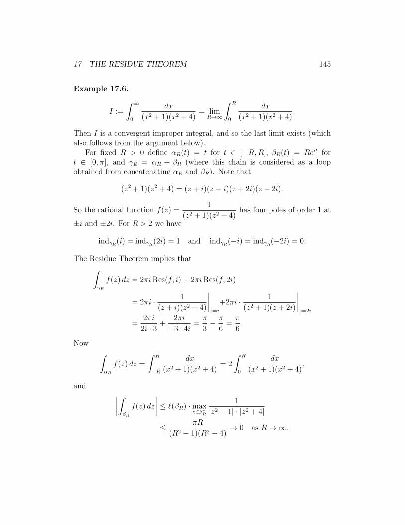
17 THE RESIDUE THEOREM 145
Example 17.6.
I :=
∫ ∞0
dx
(x2 + 1)(x2 + 4)= lim
R→∞
∫ R
0
dx
(x2 + 1)(x2 + 4).
Then I is a convergent improper integral, and so the last limit exists (whichalso follows from the argument below).
For fixed R > 0 define αR(t) = t for t ∈ [−R,R], βR(t) = Reit fort ∈ [0, π], and γR = αR + βR (where this chain is considered as a loopobtained from concatenating αR and βR). Note that
(z2 + 1)(z2 + 4) = (z + i)(z − i)(z + 2i)(z − 2i).
So the rational function f(z) =1
(z2 + 1)(z2 + 4)has four poles of order 1 at
±i and ±2i. For R > 2 we have
indγR(i) = indγR(2i) = 1 and indγR(−i) = indγR(−2i) = 0.
The Residue Theorem implies that∫γR
f(z) dz = 2πiRes(f, i) + 2πiRes(f, 2i)
= 2πi · 1
(z + i)(z2 + 4)
∣∣∣∣z=i
+2πi · 1
(z2 + 1)(z + 2i)
∣∣∣∣z=2i
=2πi
2i · 3+
2πi
−3 · 4i=π
3− π
6=π
6.
Now ∫αR
f(z) dz =
∫ R
−R
dx
(x2 + 1)(x2 + 4)= 2
∫ R
0
dx
(x2 + 1)(x2 + 4),
and ∣∣∣∣∫βR
f(z) dz
∣∣∣∣ ≤ `(βR) ·maxz∈β∗R
1
|z2 + 1| · |z2 + 4|
≤ πR
(R2 − 1)(R2 − 4)→ 0 as R→∞.

17 THE RESIDUE THEOREM 146
It follows that
I = limR→∞
∫ R
0
dx
(x2 + 1)(x2 + 4)=
1
2limR→∞
∫αR
f(z) dz
=1
2limR→∞
(∫γR
f(z) dz −∫βR
f(z) dz
)=
π
12− 1
2limR→∞
∫βR
f(z) dz =π
12.
Example 17.7.
I :=
∫ ∞0
dx√x (x+ 1)(x+ 2)
.
This is an improper integral for both integral limits 0 and ∞. It is easy tosee that it converges. One can compute I by making the substitution x = u2
and using the method from Example 17.6.We want to evaluate I based on a different method that applies to a larger
class of integrals, for example the integrals obtained by replacing√x in the
integrand by a power xα, α ∈ (0, 1). The main point here is that the squareroot function cannot be extended to holomorphic function on C∗.
We let√z be the branch of the square root with branch cut along the
non-negative real axis, normalized so that√−1 = i. Then
√reit =
√reit/2
for r > 0, t ∈ (0, 2π).Fix R > 2 and two small numbers ε > 0 and δ > 0. We define γ1(t) =
eiδt for t ∈ [ε, R], γ2(t) = Reit for t ∈ [δ, 2π − δ], γ3(t) = e−iδ(R − t) fort ∈ [0, R− ε], and γ4(t) = εe−it for t ∈ [δ, 2π − δ]. We consider the piecewisesmooth loop γ := γ1 + γ2 + γ3 + γ4 obtained from concatenation of thesepaths. The paths depend on the parameters ε, δ, and R, but we suppressthis in our notation.
Let
f(z) :=1√
z(z + 1)(z + 2)for z ∈ Ω \ −1,−2,
where Ω := C \ [0,∞). Then f is holomorphic on Ω \ −1,−2 and hassimple poles at −1 and −2. Moreover, indγ(z) = 0 for z ∈ [0,∞) and so γ is
17 THE RESIDUE THEOREM 147
null-homologous in Ω. We have indγ(−1) = indγ(−2) = 1, and
Res(f,−1) =1√
z (z + 2)
∣∣∣∣z=−1
=1√−1 · 1
=1
i,
Res(f,−2) =1√
z (z + 1)
∣∣∣∣z=−2
=1√
−2 · (−1)= − 1√
2 i.
So by the Residue Theorem,∫γ
f(z) dz = 2πi(
Res(f,−1) + Res(f,−2))
= 2π
(1− 1√
2
).
If x > 0 and z approaches x from the upper or lower half-plane, then√z →
√x or
√z → −
√x, respectively. From this one can derive that
limδ,ε→0
∫γ1
f(z) dz =
∫ R
0
dx√x (x+ 1)(x+ 2)
,
and
limδ,ε→0
∫γ3
f(z) dz =
∫ 0
R
dx
−√x (x+ 1)(x+ 2)
=
∫ R
0
dx√x (x+ 1)(x+ 2)
.
Moreover, ∣∣∣∣∫γ4
f(z) dz
∣∣∣∣ ≤ 2πε√ε (1− ε)(2− ε)
→ 0 as ε→ 0,
and ∣∣∣∣∫γ2
f(z) dz
∣∣∣∣ ≤ 2πR√R (R− 1)(R− 2)
→ 0 as R→ 0.
It follows that
2π
(1− 1√
2
)=
∫γ
f = limR→∞
(limδ,ε→0
(∫γ1
f +
∫γ2
f +
∫γ3
f +
∫γ4
f
))= lim
R→∞2
∫ R
0
dx√x (x+ 1)(x+ 2)
=
∫ ∞0
dx√x (x+ 1)(x+ 2)
= 2I,
and so I = π(1− 1√
2
).

17 THE RESIDUE THEOREM 148
Definition 17.8. Let U ⊆ C be open. A complex-valued function f is calledmeromorphic on U if there exists a set A ⊆ U such that
(i) A consists of isolated points (or equivalently, A has no limit points inthe set U),
(ii) f ∈ H(U \ A),
(iii) each point in A is a pole of f .
So a meromorphic function on U is a function that is holomorphic exceptfor isolated singularities that are poles (we may always assume that removablesingularities are absent). The possibility A = ∅ is allowed in the definition;so every holomorphic function on U is also meromorphic.
One can extend a meromorphic function to a holomorphic map f : U → Cby setting f(a) = ∞ for a pole a; it is easy to see that in this way themeromorphic functions f on U correspond precisely to the holomorphic mapsf : U → C that are not identically equal to ∞ on any component of U .
Theorem 17.9 (Argument Principle). Let U ⊆ C be a region, and f be anon-constant meromorphic function on U . Let γ : [0, 1] → U be a piecewisesmooth loop in U that is null-homologous in U and satisfies indγ(z) ∈ 0, 1for each z ∈ U \ γ∗; in addition assume that there is no zero or pole of f onγ∗.
Let Ω := z ∈ U \ γ∗ : indγ(z) = 1, and Nf and Pf be the number ofzeros and poles of f in Ω, respectively, accounted according to multiplicity.
Then Nf and Pf are finite, and
indα(0) =1
2πi
∫γ
f ′(z)
f(z)dz = Nf − Pf ,
where α := f γ.
Proof. First note that
indα(0) =1
2πi
∫α
dw
w=
1
2πi
∫ 1
0
f ′(γ(t)) · γ′(t)f(γ(t))
dt =1
2πi
∫γ
f ′(z)
f(z)dz.
If a is a zero of f of order m ∈ N, then there exists a function g holomor-phic near a such that g(a) 6= 0 and
f(z) = (z − a)mg(z) near a.

17 THE RESIDUE THEOREM 149
Then f ′(z) = m(z − a)m−1g(z) + (z − a)mg′(z), and so
f ′(z)
f(z)=
m
z − a+g′(z)
g(z)near a.
Hence f ′/f has a simple pole at a, and
Res(f ′/f, a) = m = multiplicity of the zero a.
Similarly, if a is a pole of f , then there exists a function g holomorphicnear a such that g(a) 6= 0 and
f(z) =1
(z − a)mg(z) near a.
Then
f ′(z) = − m
(z − a)m+1g(z) +
1
(z − a)mg′(z),
and sof ′(z)
f(z)=−mz − a
+g′(z)
g(z)near a.
Hence f ′/f has a simple pole at a, and
Res(f ′/f, a) = −m = −multiplicity of the pole a.
The set Ω = z ∈ U \ γ∗ : indγ(z) = 1 ⊆ U is open as follows fromTheorem 14.14. Let A be the set of zeros and poles of f in Ω, and B be theset of the remaining zeros and poles of f in U . Both A and B consists ofisolated points. If U := U \B, then U is an open set and γ is null-homologous
in U .Note that the set A is finite (which implies that Nf and Pf are finite);
indeed, A is a bounded set, because it must be disjoint from the unboundedcomponent of C \ γ∗; so if A were infinite, then it had a limit point w.Then necessarily w ∈ ∂U ⊆ C \ U , and so indγ(w) = 0, because γ isnull-homologous in U . Then indγ(a) = 0 for points a ∈ A close to w byTheorem 14.14. This is impossible as indγ(a) = 1 for a ∈ A.
Since f ′/f ∈ H(U \ A) we can apply the Residue Theorem and obtain
1
2πi
∫γ
f ′(z)
f(z)dz =
∑a∈A
Res(f ′/f, a) = Nf − Pf .
17 THE RESIDUE THEOREM 150
Theorem 17.10 (Rouche’s Theorem). Let U ⊆ C be a region, and f and gbe non-constant holomorphic functions on U . Let γ : [0, 1]→ U be a piecewisesmooth path that is null-homologous in U and satisfies indγ(z) ∈ 0, 1 foreach z ∈ U \ γ∗; in addition assume that there is no zero of f on γ∗.
Let Ω = z ∈ U \ γ∗ : indγ(z) = 1, and Nf and Ng be the numbers ofzeros of f and g in Ω, respectively, counted according to multiplicity.
If|g(z)− f(z)| < |f(z)| for all z ∈ γ∗, (72)
then Nf = Ng.
So if the functions f and g are sufficiently close on γ∗, then they have thesame number of zeros in Ω.
Proof. Note that (72) implies that g(z) 6= 0 for z ∈ γ∗. Hence we can applythe Argument Principle to both f and g and conclude Nf = indfγ(0) andNg = indgγ(0). The statement will follow from the homotopy invariance ofwinding numbers if we can show that the loops f γ and g γ are homotopicin C∗.
We define H : [0, 1]× [0, 1]→ C∗ by
H(s, t) = f(γ(s)) + t(g(γ(s))− f(γ(s))
)for s, t ∈ [0, 1].
Then H is continuous. By (72) we have
|H(s, t)| ≥ |f(γ(s))| − |g(γ(s))− f(γ(s))| > 0
for all s, t ∈ [0, 1]. So H maps into C∗. Since γ is a loop, and so γ(0) = γ(1),we have H(0, t) = H(1, t) for all t ∈ [0, 1]. So H(·, t) is a loop for all t ∈ [0, 1].Since H(·, 0) = f γ and H(·, 1) = g γ, the loops f γ and g g are indeedhomotopic in C∗ as desired.
Example 17.11. (a) Consider the polynomial g(z) = z9−2z6 +z4−9z2 +3.Then one can use Rouche’s Theorem to show that g has precisely two zeros(possibly one double zero) in the unit disk D. Indeed, in Theorem 17.10 welet U := C, γ(t) := e2πit for t ∈ [0, 1], and f(z) := −9z2. Note that thenΩ = z ∈ C \ γ∗ : indγ(z) = 1 = D, and that for z ∈ γ∗ = ∂D we have
|g(z)− f(z)| = |z9 − 2z6 + z4 + 3| ≤ |z|9 + 2|z|6 + |z|4 + 3 = 7
< 9 = | − 9z2| = |f(z)|.
17 THE RESIDUE THEOREM 151
So Ng, the number of zeros of g in D, is equal to Nf = 2, the number of zerosof f in D.
(b) One can derive the Fundamental Theorem of Algebra from Rouche’sTheorem. If
g(z) = zn + an−1zn−1 + · · ·+ a0
is a polynomial of degree n ≥ 1, we let f(z) = zn, and γ(t) = Re2πit fort ∈ [0, 1]. For sufficiently large R ≥ 1 and M := |an−1| + · · · + |a0| we havefor z ∈ γ∗,
|g(z)− f(z)| = |an−1zn−1 + · · ·+ a0| ≤MRn−1 < Rn = |z|n = |f(z)|.
Since f has n zeros in D(0, R), the polynomial g has also n ≥ 1 zeros.
18 Normal families
Definition 18.1. Let X and Y be metric spaces, and f : X → Y andfn : X → Y for n ∈ N be maps.
(a) We say that fn converges to f locally uniformly on X if for all p ∈ Xthere exists a neighborhood U of p (i.e., p ∈ int(U)) such that fn|U →f |U uniformly on U .
(b) We say that fn converges to f compactly on X or uniformly on compactsubsets of X if for all compact sets K ⊆ X we have fn|K → f |Kuniformly on K.
We use the notation fn → f locally uniformly on X or fn → f compactlyon X (as n→∞).
A metric space X is said to be locally compact if each point p ∈ X has acompact neighborhood U ⊆ X.
Proposition 18.2. Let X and Y be metric spaces, and f : X → Y andfn : X → Y for n ∈ N be maps. Suppose that X is locally compact. Then thefollowing two conditions are equivalent:
(i) fn → f locally uniformly on X.
(ii) fn → f compactly on X.
Moreover, if (i) or (ii) is true and fn is continuous for each n ∈ N, then fis also continuous.
Proof. (i) ⇐ (ii): Suppose (ii) is true. Let K be a arbitrary compact subsetof X. Then for each p ∈ K there exists a neighborhood Up ⊆ X such thatfn|Up → f |Up uniformly on Up. By compactness of K there exist finitelymany points, say p1, . . . , pm ∈ K such that K ⊆ Up1 ∪ · · · ∪ Upm . Thenfn → f uniformly on K ⊆ Up1 ∪ · · · ∪ Upm .
(i) ⇒ (ii): Suppose (i) is true, and let p ∈ X be arbitrary. Since Xis locally compact, there exists a compact neighborhood U of p. By ourhypothesis, fn → f uniformly on U . Hence every point has a neighborhoodon which the convergence fn → f is uniform. Hence fn → f locally uniformlyon X.
152

18 NORMAL FAMILIES 153
The last statement follows from a well-known argument. We denote themetric on X and Y by d and ρ, respectively. Suppose that fn → f locallyuniformly on X, and that fn is continuous for each n ∈ N. Let p ∈ X andε > 0 be arbitrary. We can find a neighborhood U ⊆ X of p such that fn → funiformly on U . Hence there exist N ∈ N such that
ρ(f(q), fN(q)) < ε/3 for all q ∈ U.
Since fN is continuous at p and U is a neighborhood of p, there exists δ >0 such that for each point q ∈ X with d(p, q) < δ we have q ∈ U andρ(fN(q), fN(p)) < ε/3. For such points q we then have
ρ(f(q), f(p)) < ρ(f(q), fN(q)) + ρ(fN(q), fN(p)) + ρ(fN(p), f(p))
< ε/3 + ε/3 + ε/3 = ε.
This shows that f is continuous at p. Since p was arbitrary, f is continuouson X.
We will be mostly interested in the case where X is an open subset ofC (equipped with the Euclidean metric), or an open subset of C (equipped
with the chordal metric), and Y = C or Y = C. In these cases, X is locallycompact and so the notions of locally uniform and compact convergenceare equivalent. We will use this fact repeatedly in the following withoutmentioning it explicitly.
Example 18.3. (a) Let f(z) =∞∑k=0
ak(z−z0)k be a power series with positive
radius of convergence R > 0. Let fn(z) =n∑k=0
ak(z − z0)k be the nth partial
sum of the power series. We know that fn → f uniformly on compact subsetsof B := B(z0, R), and so fn → f locally uniformly on B.
(b) Let f(z) =∞∑
k=−∞
ak(z− z0)k be a Laurent series that converges on an
annulus A = z ∈ C : R1 < |z − z0| < R2. We write f(z) = g(z) + h(z),
where g(z) =∞∑k=0
ak(z − z0)k and h(z) =−1∑
k=−∞
ak(z − z0)k.
18 NORMAL FAMILIES 154
If gn(z) =n∑k=0
ak(z− z0)k and hn(z) =−1∑
k=−n
ak(z− z0)k for n ∈ N, then it
follows from (a) and the discussion in Remark 16.11 that gn → g and hn → h
locally uniformly on A. In particular, if fn(z) =n∑
k=−n
ak(z − z0)k for n ∈ N0,
then fn → f locally uniformly on A.
Theorem 18.4. Let U ⊆ C be open, f : U → C, and fn ∈ H(U) for n ∈ N.Suppose that fn → f locally uniformly on U . Then f ∈ H(U). Moreover,
for each k ∈ N we have f(k)n → f (k) locally uniformly on U .
So locally uniform limits of holomorphic functions are holomorphic, andtaking derivatives is compatible with taking locally uniform limits.
Proof. The function f is continuous on U as a locally uniform limit of con-tinuous functions (Proposition 18.2). The holomorphicity of f now followsfrom Morera’s Theorem; indeed, if ∆ ⊆ U is an arbitrary closed orientedtriangle in U , then fn → f uniformly on ∂∆. Hence∫
∂∆
f = limn→∞
∫∂∆
fn︸ ︷︷ ︸=0
= 0.
For the second statement is enough to establish the case k = 1; the generalcase then follows from this by repeated application.
So let z0 ∈ U be arbitrary. Pick r > 0 such that B(z0, r) ⊆ U . Letγ(t) = z0 + reit for t ∈ [0, 2π]. Then for all z ∈ B(z0, r/2),
|f ′n(z)− f ′(z)| = 1
2π
∣∣∣∣∫γ
fn(w)− f(w)
(w − z)2dw
∣∣∣∣≤ r
(r/2)2max
w∈∂B(z0,r)|fn(w)− f(w)|
=4
rmax
w∈∂B(z0,r)|fn(w)− f(w)| → 0 as n→∞.
This estimate implies that f ′n → fn uniformly on B(z0, r/2), and it followsthat f ′n → f locally uniformly on U .
18 NORMAL FAMILIES 155
Example 18.5. As in Example 18.3 let f(z) =∞∑k=0
ak(z − z0)k be a power
series convergent on a disk B, and fn be the nth partial sum of the powerseries. Then fn → f locally uniformly on B, and so by the last theoremf ′n → f ′ locally uniformly on B. This amounts to the statement that a powerseries can be differentiated term-by-term (already proved in Theorem 5.9);indeed, for z ∈ B, we have
f ′(z) = limn→∞
f ′n(z) = limn→∞
d
dz
( n∑k=0
ak(z − z0)k)
= limn→∞
n∑k=0
d
dz
(ak(z − z0)k
)= lim
n→∞
n∑k=1
kak(z − z0)k−1
=∞∑k=1
kak(z − z0)k−1 =∞∑k=0
(k + 1)ak+1(z − z0)k.
Similarly, a convergent Laurent series can be differentiated term-by-term.
Theorem 18.6 (Hurwitz’s Theorem). Let U ⊆ C be a region, f ∈ H(U),and fn ∈ H(U) for n ∈ N. Suppose that fn → f locally uniformly on U . Iffn is injective for each n ∈ N, then f is constant or also injective.
Proof. We argue by contradiction and assume that under the given hypothe-ses, f is neither constant nor injective. Then there exist z1, z2 ∈ U , z1 6= z2,such that f(z1) = f(z2). Without loss of generality, we may assume thatf(z1) = f(z2) = 0.
We can choose a small r > 0 such that B1 := B(z1, r) ⊆ U , B2 :=B(z2, r) ⊆ U , B1∩B2 = ∅, and so that f has no zeros on ∂B1∪∂B2 (a choicesatisfying the last condition is possible, because f is non-constant and so thezeros of f are isolated points). Then m := inf|f(z)| : z ∈ ∂B1 ∪ ∂B2 > 0.
Since fn → f uniformly on ∂B1 ∪ ∂B2, we can find N ∈ N such that
|fN(z)− f(z)| < m ≤ |f(z)| for all z ∈ ∂B1 ∪ ∂B2.
By Rouche’s Theorem fN has the same number of zeros as f in int(B1) andin int(B2). So fn has at least one zero, say w1, in int(B1), and one, say w2
in int(B2). Then w1 6= w2, and fN(w1) = 0 = fN(w2). This contradicts thefact that fN is injective.

18 NORMAL FAMILIES 156
Definition 18.7 (Normal families). Let U ⊆ C be open, and F be a familyof complex-valued continuous functions on U . We say that F is a normalfamily if every sequence fn of functions in F has a subsequence fnk
thatconverges to some function f : U → C locally uniformly on U .
We do not require that the sublimit f belongs to F .
Definition 18.8. Let U ⊆ C be open, and F be a family of complex-valuedcontinuous functions on U . Then the family F is called
(a) equicontinuous at a point z0 ∈ U if for all ε > 0 there exists δ > 0 suchthat for all f ∈ F and all z ∈ U we have the implication
|z − z0| < δ ⇒ |f(z)− f(z0)| < ε.
(b) uniformly bounded on A ⊆ U if there exists M ≥ 0 such that for allf ∈ F and all z ∈ A we have
|f(z)| ≤M.
The family is called uniformly bounded at z0 ∈ U if it is uniformlybounded on A = z0. It is called locally uniformly bounded if everypoint z0 ∈ U has a neighborhood on which F is uniformly bounded.
The following theorem is a version of the Arzela-Ascoli Theorem. It givesa complete characterization of normal families.
Theorem 18.9 (Arzela-Ascoli). Let U ⊆ C be open, and F be a family ofcomplex-valued continuous functions on U . Then F is a normal family ifand only if F is equicontinuous and uniformly bounded at each point z0 ∈ U .
Proof. ⇒: Suppose F is a normal family. To show that is equicontinuousand uniformly bounded at each point in U we argue by contradiction.
Suppose F is not uniformly bounded at some point z0 ∈ U . Then for eachn ∈ N there exists fn ∈ F such that |fn(z0)| ≥ n. Then the sequence fncannot have a subsequence that converges locally uniformly on U , because nosubsequence even has a pointwise limit at z0. This contradicts the normalityof F .
18 NORMAL FAMILIES 157
Suppose F is not uniformly bounded at some point z0 ∈ U . Then thereexists ε0 > 0 (“bad ε”) such that for each n ∈ N there exists fn ∈ F andzn ∈ U with |zn − z0| < 1/n such that
|fn(zn)− fn(z0)| ≥ ε0 > 0. (73)
Since F is normal we may assume (by passing to a subsequence if necessary)that fn converges to some continuous function f : U → C locally uniformly onU . Then fn(z0)→ f(z0) as n→∞. Since zn → z0, the convergence fn → fis locally uniform, and f is continuous at z0, we also have fn(zn) → f(z0)(excercise!). Hence |fn(zn)− fn(z0)| → 0 as n→∞, contradicting (73).⇐: Suppose F is equicontinuous and uniformly bounded at each point in
U . Let fn be an arbitrary sequence in F . In order to establish that F is anormal family we have to show that fn has a subsequence that convergeslocally uniformly on U .
We choose a countable dense subset D := pn : n ∈ N in U (for ex-ample the set of all points in U whose real and imaginary parts are rationalnumbers). Since F is uniformly bounded at each point in U , for each k ∈ Nthe sequence fn(pk) is bounded. Hence we can find a subsequence f1nof fn such that f1n(p1) converges. Using the boundedness of f1n(p2),we can find a subsequence f2n of f1n such that f2n(p2) converges. Re-peated this argument, for each k ∈ N we can find a subsequence fkn offn such that fkn(pk) converges and such that fk+1n is a subsequenceof fkn. Consider the “diagonal” subsequence gn given by gn := fnn forn ∈ N. Then gn is a subsequence of fn, and, if we disregard finitelymany terms, gn(pk) is a subsequence of fkn(pk) for each k ∈ N. Hencegn(p) converges for each p ∈ D.
Claim. For each compact set K ⊆ U and each ε > 0 there exists N ∈ Nsuch that
|gk(z)− gn(z)| ≤ ε for all z ∈ K and all k, n ∈ N with k, n ≥ N . (74)
To see this, let ε > 0 and K ⊆ U be compact. Since F and hence also thesubfamily gn is equicontinuous at each point in U , for each w ∈ K thereexists δw > 0 such that
|gn(z)− gn(w)| ≤ ε/3 for all n ∈ N and all z ∈ B(w, δw). (75)
Since K is compact there exist finitely many points w1, . . . , wm such thatthe balls Bj := B(wj, δwj
), j = 1, . . . ,m, cover K. Since D is dense in U ,

18 NORMAL FAMILIES 158
for each j ∈ 1, . . . ,m we can pick a point p′j ∈ D ∩ Bj. Then gn(p′j)converges, and so is a Cauchy sequence for each j = 1, . . . ,m. Hence thereexists N ∈ N such that
|gk(p′j)− gn(p′j)| ≤ ε/3 whenever j ∈ 1, . . . ,m and k, n ≥ N . (76)
Now let z ∈ K and k, n ∈ N with k, n ≥ N be arbitrary. Then there existsj ∈ 1, . . . ,m with z ∈ Bj. Combining (75) and (76) we obtain
|gk(z)− gn(z)| ≤ |gk(z)− gk(p′j)|+ |gk(p′j)− gn(p′j)|+ |gn(p′j)− gn(z)|≤ ε/3 + ε/3 + ε/3.
This establishes the claim.The claim implies that gn converges locally uniformly on U to some
limit function. Namely, first it shows that for each z ∈ U the sequencegn(z) is a Cauchy sequence, and hence converges, say gn(z) → g(z) ∈ Cas n → ∞. Moreover, letting k → ∞ in (74) we see that the convergencegn → g is uniform on each compact set K ⊆ U . So the subsequence gn ofour original sequence fn converges to some limit function locally uniformlyon U . Hence F is a normal family.
It seems that this theorem completely solves all questions concerningnormal families. In practice it often not so easy to establish the relevantequicontinuity and uniform boundedness conditions in order to establish thenormality of a family. For example, let S be the family of all holomorphicfunctions f on the unit disk D that are injective and satisfy f(0) = f ′(0)−1 =0. Then one can show that S is a normal family, but it is not immediatelyclear how to verify the conditions in the Arzela-Ascoli theorem.
A condition that guarantees that a family is normal is called a normalitycriterion. The following theorem provides the basic normality criterion forholomorphic functions.
Theorem 18.10 (Montel’s “Little” Theorem). Let U ⊆ C be open, and Fbe a family of holomorphic functions on U . Then F is a normal family ifand only if F is locally uniformly bounded.
Proof. ⇒: This implication follows from the Arzela-Ascoli Theorem (even ifwe replace the assumption that the functions in the family are holomorphicby the weaker assumption that they are only continuous). Indeed, if thefamily is normal, then it is equicontinuous and uniformly bounded at each

18 NORMAL FAMILIES 159
point of U . This in turn implies that the family is locally uniformly boundedon U .⇐: By the Arzela-Ascoli Theorem it suffices to show that F is equicon-
tinuous at each point in U . So let z0 ∈ U be arbitrary. We can pick r > 0such that B(z0, r) ⊆ U and such that F is uniformly bounded on B(z0, r).So there exists M ≥ 0 such that
|f(z)| ≤M whenever f ∈ F and z ∈ B(z0, r).
Define γ(t) = z0 + reit for t ∈ [0, 2π], and let z ∈ B(z0, r/2) and f ∈ F bearbitrary. Then
|f(z)− f(z0)| = 1
2π
∣∣∣∣∫γ
f(w)
(1
w − z− 1
w − z0
)dw
∣∣∣∣≤ 1
2π· 2πr · max
w∈∂B(z0,r)
|f(w)| · |z − z0||w − z| · |w − z0|
= r · M
(r/2)r|z − z0| =
2M
r|z − z0|.
Since M is independent of f and z, the equicontiuity of F at z0 immediatelyfollows.
Remark 18.11. One can prove results similar to the one established forholomorphic functions also for meromorphic functions (considered as holo-
morphic maps into C). In this case one uses the chordal metric in order tomeasure distances in the target.
One can show that a locally uniform limit of meromorphic functions on aregion is again meromorphic (one has to allow the function that is identicallyequal to ∞ here).
The notion of a normal family of continuous maps into C is defined inthe same way as in Definition 18.7. The corresponding version of the Arzela-Ascoli Theorem then says that a family of such maps F is normal if and onlyif it is equicontiunous at each point. The proof of this statement is identicalto the proof of Theorem 18.9. The uniform boundedness condition is notrelevant here since every sequence in C has a convergent subsequence.
When one considers normal families one has to be careful about the metricused in the target. Every holomorphic function on a region U can also beconsidered as a map into C ⊇ C. If a family of holomorphic functions ona region is U is normal as considered as a family of maps into C, then it is
18 NORMAL FAMILIES 160
also normal as considered as a family of maps into C, but the converse is nottrue. On can show that a family F ⊆ H(U) is normal in the latter sense,if and only if every sequence fn in F has a subsequence that convergeslocally uniformly to the constant function ∞ or to a function holomorphicon U . Often this is taken as the definition of a normal family of holomorphicfunctions.
One can formulate sufficient conditions for the normality of a familyof meromorphic functions that are similar to Montel’s Theorem 18.10. Astronger statement is Montel’s “Big” Theorem: if each function in a fam-ily of meromorphic functions on a region omits three distinct fixed valuesa, b, c ∈ C, then it is normal. For example, a family of holomorphic functionsomitting 0 and 1 (the third omitted value is ∞ here) is normal (as a family
of maps into C).
19 The Riemann Mapping Theorem
Lemma 19.1. Let Ω ⊆ C be a simply connected region, Ω 6= C. Then thereexists a conformal map g : Ω → Ω, where Ω is a Koebe region, i.e., Ω is asimply connected region with 0 ∈ Ω ⊆ D.
Proof. Pick a ∈ C \ Ω. Then z 7→ z − a is a zero-free holomorphic functionon Ω. So by Corollary 15.9 this function has a holomorphic square root S,i.e., S ∈ H(Ω) and
S(z)2 = z − a for all z ∈ Ω.
The function S is injective on Ω: if z1, z2 ∈ Ω are arbitrary, then we have theimplications
S(z1) = S(z2) ⇒ S(z1)2 = S(z2)2
⇒ z1 − a = z2 − a ⇒ z1 = z2.
So S is a holomorphic bijection S : Ω → U := S(Ω) onto its image U , andin particular a conformal map (Corollary 9.6). The set U is a region (seeCorollary 9.5). It has the following property: if w ∈ U , then −w 6∈ U ;indeed, suppose w,−w ∈ U . Then there exist z1, z2 ∈ Ω such that w = S(z1)and −w = S(z2). Hence
z1 − a = S(z1)2 = w2 = S(z2)2 = z2 − a,
and so z1 = z2. This implies
w = S(z1) = S(z2) = −w,
and gives w = 0. This is impossible, because the map z 7→ z − a = S(z)2,and hence also S, is zero-free on Ω.
Since U is open, there exists w0 ∈ U , and r > 0 such that B(w0, r) ⊆ U .Then B(w1, r) ∩ V = ∅, where w1 := −w0.
Consider the Mobius transformation T : U → C,
T (w) :=r
w − w1
.
Then T : U → V := T (U) is a conformal map of U onto its image V =T (U) ⊆ D. Pick u0 ∈ V , and let
R(u) :=u− u0
1− u0u, u ∈ D.
161

19 THE RIEMANN MAPPING THEOREM 162
Then R ∈ Aut(D), and 0 ∈ Ω := R(T (U)) ⊆ D. So we have the sequence ofholomorphic bijections
ΩS−→ U
T−→ VR−→ Ω ⊆ D.
Then g := R T S is a holomorphic bijection of Ω onto Ω, and hence aconformal map from Ω onto Ω. The set Ω is a region with 0 ∈ Ω. Moreover,Ω is simply connected, because this property of a region is invariant underconformal maps. So Ω is a Koebe region, and g is a conformal map from Ωonto Ω.
If one replaces the condition that the regions in the previous statement aresimply connected by the condition that every zero-free holomorphic functionon the region has a holomorphic square root, then the previous proof goesthrough with the conclusion that Ω satisfies the latter property. Note thisproperty of a region is invariant under conformal maps of the region.
Lemma 19.2. Let Ω ⊆ D be a Koebe region, and
S(Ω) := f : Ω→ f(Ω) conformal, f(Ω) ⊆ D, f(0) = 0.
Thenα := sup|f ′(0)| : f ∈ S(Ω) (77)
is attained as a maximum, i.e., there exists f0 ∈ S(Ω) such that |f ′(0)| ≤|f ′0(0)| = α for all f ∈ S(Ω).
Proof. Note that α ≥ 1, because idΩ ∈ S(Ω). Let fn be a sequence in S(Ω)with |f ′n(0)| → α. Montel’s Theorem implies that by passing to a subsequenceif necessary we may assume that fn → f0 ∈ H(Ω) locally uniformly onΩ. Then f0(0) = lim
n→∞fn(0) = 0, and |f ′0(0)| = lim
n→∞|f ′n(0)| = α > 0.
In particular, f0 is not a constant function. By Hurwitz’s Theorem f0 isinjective, and so f0 is a conformal map of Ω onto f0(Ω) ⊆ D. Since f0(Ω)is open, we must have f0(Ω) ⊆ D. Then f0 ∈ S(Ω) and |f ′0(0)| = α asdesired.
Lemma 19.3. Let Ω ⊆ D be a Koebe region, and f0 ∈ S(Ω) be a mapfor which the supremum in (77) is attained. Then f0(Ω) = D, i.e., f is aconformal map from Ω onto D.

19 THE RIEMANN MAPPING THEOREM 163
Proof. We argue by contradiction; so suppose U0 := f0(Ω) 6= D. Since0 ∈ U0 ⊆ D, there exists a 6= 0 such that a ∈ D \ U0. Let R be the Mobiustransformation given by
R(u) :=u− a1− av
.
Then R ∈ Aut(D), and so R is a conformal map from U0 onto U1 := R(U0) ⊆D. Then U1 is a simply connected region. Since R(a) = 0, we have 0 6∈ U1.So by Corollary 15.9 there exists a homolomorphic branch of the square rootfunction on U1; i.e., a holomorphic map S : U1 → C such that
S(v)2 = v for v ∈ U1.
Then for v ∈ U1 we have |S(v)|2 = |v| < 1, and so U2 := S(U1) ⊆ D.Moreover, S is injective on U1; indeed, if for v1, v2 ∈ Ω, we have S(v1) =S(v2), then v1 = S(v1)2 = S(v2)2 = v2. It follows that S is a conformal mapof U1 onto the simply connected region U2 := S(U1) ⊆ D.
Let b := S(R(0)) ∈ S(U1) ⊆ U2 ⊆ D, and T be the Mobius transformationgiven by
T (w) :=w − b1− bw
.
Then T ∈ Aut(D), and so T is a conformal map from U2 onto the simplyconnected region U3 := T (U2) ⊆ D. Note that 0 = T (b) ∈ T (U2) = U3, andso U3 is a Koebe region.
We have constructed conformal maps
U0R−→ U1
S−→ U2T−→ U3.
Consider the composition g := R S T . Then g is a conformal map fromU0 onto U3 with
g(0) = (T S R)(0) = T (b) = 0.
Moreover,
R′(u) =1− |a|2
(1− au)2, |S ′(v)| = 1
2√|v|, T ′(w) =
1− |b|2
(1− bw)2,
and so
|R′(0)| = 1− |a|2, |S ′(R(0))| = |S(−a)| = 1
2√|a|, |T ′(b)| = 1
1− |b|2.

19 THE RIEMANN MAPPING THEOREM 164
Note also that
|b|2 = |S(R(0))2| = |S(−a)2| = | − a| = |a| < 1.
Putting this all together gives
|g′(0)| =∣∣T ′(S(R(0))
)∣∣ · |S ′(R(0))| · |R′(0)| = |T ′(b)| · |S ′(−a)| · |R′(0)|
=1
1− |b|2· 1
2√|a|· (1− |a|2) =
1− |a|2
2√|a| (1− |a|)
=1 + |a|2√|a|
= 1 +(1−
√|a|)2
2√|a|
> 1.
Then f := g f0 is a conformal map of Ω onto the Koebe region g(f0(Ω)) =g(U0) = U3, and f(0) = g(f0(0)) = g(0) = 0; so f ∈ S(Ω), but
|f ′(0)| = |g′(0)| · |f ′0(0)| > |f ′0(0)|.
This contradicts the maximality property of f0.
Remark 19.4. (a) Again the relevant property of Ω in the previous proofwas that every zero-free holomorphic function on Ω has a holomorphic squareroot (which transfers to U0 = f0(Ω) and all the other regions considered).
(b) The computation in the previous proof make it seem to be a fortunatecoincidence that we get the crucial inequality |g′(0)| > 1. One can actuallysee that this inequality must be true almost without any computation if one
consider how the hyperbolic length element dsh =2|dz|
1− |z|2is distorted by
the map. If f is a holomorphic map defined near a point z ∈ D and hasvalues in D, then this distortion at z is measured by the derivative of f withrespect to the hyperbolic metric given by
Dh(f)(z) :=f ∗(dsh)
dsh=
(1− |z|2)|f ′(z)|1− |f(z)|2
.
This derivative has the expected properties (chain rule, behavior for inversemaps, etc.). Note also that if f(0) = 0 then Dh(f)(0) = |f ′(0)|.
We know that Dh(ϕ)(z) ≡ 1 if ϕ ∈ Aut(D). Moreover, if f : D → D isholomorphic, but f 6∈ Aut(D), then Dh(f)(z) < 1 for all z ∈ D. So if g isa branch of the inverse f−1 defined near a point z ∈ D, then Dh(g)(z) =

19 THE RIEMANN MAPPING THEOREM 165
Dh(f)(g(z))−1 > 1. In particular, this is true for the branch S of the squareroot function (an inverse branch of z 7→ z2 mapping D into D) used in theprevious proof. This can also verified by direct computation:
|S ′(z)| = 1
2√|z|
and |S(z)|2 = |z|,
which implies
Dh(S)(z) =(1− |z|2)|S ′(z)|
1− |S(z)|2=
1− |z|2
2√|z| (1− |z|)
=1 + |z|2√|z|
> 1,
whenever z ∈ D.In the previous proof, the function g was given as g := R S T , where
R, T ∈ Aut(D). Moreover, g(0) = 0, and so
|g′(0)| = Dh(g)(0) = Dh(R)(S(T (0))
)·Dh(S)(T (0)) ·Dh(T )(0)
= Dh(S)(T (0)) > 1.
Theorem 19.5 (Riemann Mapping Theorem). Let Ω ⊆ C be a simply con-nected region, Ω 6= C. Then there exists a conformal map f : Ω → D of Ωonto D.
If z0 ∈ Ω is arbitrary, then f can be chosen so that
f(z0) = 0 and f ′(z0) > 0. (78)
Moreover, with this normalization the map f is uniquely determined.
Proof. By Lemma 19.1 there exists a conformal map h1 : Ω → Ω onto aKoebe region Ω. By Lemma 19.3 there exists a conformal map h2 : Ω → D.Then f := h2 h1 is a conformal map from Ω onto D.
If z0 ∈ Ω is arbitrary, then w0 := f(z0) ∈ D. For fixed θ ∈ [0, 2π] to bedetermined momentarily, consider the Mobius transformation
ϕ(w) = eiθw − w0
1− w0w.
Then ϕ ∈ Aut(D), and ϕ(w0) = 0. So f := ϕ f is a conformal map from Ω
onto D with f(0) = ϕ(w0) = 0. Moreover,
f ′(z0) = ϕ′(w0) · f ′(z0) = eiθf ′(z0)
1− |w0|2.
19 THE RIEMANN MAPPING THEOREM 166
By choosing θ ∈ [0, 2π] appropriately, we get f ′(z0) > 0. Then f is a confor-mal map of Ω onto D with the desired normalization.
Suppose f1 and f2 are two conformal maps from Ω onto D satisfying thenormalization (78). Then ψ := f2 f−1
1 ∈ Aut(D), ψ(0) = 0, and
ψ′(0) = f ′2(f−11 (0)) · (f−1
1 )′(0) =f ′2(z0)
f ′1(z0)> 0.
So ψ(z) = eiαz, where α ∈ [0, 2π) and ψ′(0) = eiα > 0. This implies α = 0,ψ = idD, and f1 = f2.
Based on the remarks after Lemmas 19.1 and 19.3 the argument in theprevious proof actually shows that if Ω ⊆ C, Ω 6= C, is a region such thatevery zero-free holomorphic function has a holomorphic square root, then Ωis conformally equivalent to D, i.e., there exists a conformal map of Ω ontoD.
Example 19.6. In some simple cases the Riemann map, i.e., the conformalmap of the simply connected region of Ω onto D can be found explicitly. Hereare two examples.
(a) Let Ω := reiα : 0 < r < 1, 0 < α < π/4. The region Ω isconvex, and hence simply connected. The Riemann map can be found as acomposition of conformal maps U0 = Ω→ U1 → U2 → U3 → U4 = D, where
z ∈ U0 7→ s := z4 ∈ U1 := s ∈ C : |s| < 1, Im s > 0,
s ∈ U1 7→ t :=1 + s
1− s∈ U2 := t ∈ C : Re t > 0, Im t > 0,
t ∈ U2 7→ u := t2 ∈ U3 := u ∈ C : Im u > 0,
u ∈ U3 7→ w :=1 + iu
1− iu∈ U4 := D.
So w = f(z) =1 + i
(1+z4
1−z4)2
1− i(
1+z4
1−z4)2 gives a conformal map of Ω onto D.
(b) Let Ω := z ∈ C : −π < Im z < π \ (−∞, 0]. The region Ω isstarlike with respect to p = 1. This means that [p, z] ⊆ Ω for all z ∈ Ω andimplies that Ω is simply connected. Again the Riemann map can be found
19 THE RIEMANN MAPPING THEOREM 167
as a composition of conformal maps U0 = Ω→ U1 → U2 → U3 = D. Here
z ∈ U0 7→ u := ez ∈ U1 := C \ (−∞, 1],
u ∈ U1 7→ v :=√u− 1 ∈ U2 := v ∈ C : Re v > 0 (principal branch),
v ∈ U2 7→ w :=1− v1 + v
∈ U3 := D.
So w = f(z) =1−√ez − 1
1 +√ez − 1
gives a conformal map of Ω onto D.
Remark 19.7. Since the upper half-plane H := z ∈ C : Im z > 0 isconformally equivalent to D, for every simply connected region Ω ⊆ C, Ω 6=Ω, there exists a conformal map f : H → Ω. A general class of simplyconnected regions Ω for which such a map f can be obtained quite explicitlyare those bounded by polygons (consisting of straight line segments).
Suppose that ∂Ω is a finite union of line segments ∂Ω =n⋃k=1
[pk, pk+1] with
pairwise disjoint interiors, where pn+1 = p1, and let αkπ be the interior angleat the corner pk with αk ∈ (0, 2). Then one can show that there exist pointsa1 < a2 < · · · < an on the real axis and constants A ∈ C and B ∈ C \ 0such that f is given by the Schwarz-Christoffel map
f(z) = A+B
∫[0,z]
n∏k=1
(ζ − ak)αk−1 dζ.
Here one has to choose suitable branches of the power functions, for examplethose that attain positive values for large positive values of ζ. Moreover, thisconformal map of H onto Ω has a continuous extension to H = z ∈ C :Im z ≥ 0 ∪ ∞ such that f(ak) = pk for k = 1, . . . , n.
For example, let k ∈ (0, 1), and define
f(z) =
∫[0,z]
dζ√(1− ζ2)(1− k2ζ2)
for z ∈ H. Here the branch of the root is such that for ζ = 0 we have√
1 = 1.One can show that then f is homeomorphism of H onto the rectangle
R := w ∈ C : −K ≤ Re w ≤ K, 0 ≤ Im w ≤ K ′

19 THE RIEMANN MAPPING THEOREM 168
and a conformal map of H onto int(R). The quantities K and K ′ are givenby complete elliptic integrals of the first kind:
K =
∫ π/2
0
dt√1− k2 sin2 t
, and K ′ =
∫ π/2
0
dt√1− k′2 sin2 t
,
where k′ :=√
1− k2 ∈ (0, 1). The map f sends the points ±1 and ±1/kto the corners of R; more precisely, we have f(±1) = ±K and f(±1/k) =±K + iK ′.
Theorem 19.8 (Schwarz Reflection Principle). Let U+ ⊆ H+ := z ∈ C :Im z > 0 be open, U− := z : z ∈ U+, and α ⊆ R be open (as a subset ofR). Define Ω = U+ ∪ α ∪ U−, and assume that α ⊆ int(Ω) (which impliesthat Ω is open).
Let f : U+ ∪ α→ C be continuous and holomorphic on U+. If f(α) ⊆ R,then the extension F : Ω→ C of f given by
F (z) =
f(z) for z ∈ U+ ∪ α,
f(z) for z ∈ U−,
is holomorphic on Ω.If in addition f is injective on U+ ∪ α and f(U+) ⊆ H+, then F is
injective on Ω, and so F is a conformal map of Ω onto its image F (Ω).
Proof. Obviously, F is continuous on Ω. Moreover, F |U− is holomorphic onU−. Indeed, if a ∈ U− is arbitrary, then a ∈ U+, and so f has a power seriesrepresentation
f(z) =∞∑n=0
an(z − a)n for z near a.
Then
F (z) = f(z) =∞∑n=0
an(z − a)n for z near a,
and so the holomorphicity of F near a follows.The holomorphicity of F on the whole set Ω easily follows from its con-
tinuity on Ω, its holomorphicity of F on U+ ∪ U−, and Morera’s Theorem.Finally, if f is injective on U+ ∪ α and f(U+) ⊆ H+, then F is injective
on U− and F (U−) ⊆ H− := z ∈ C : Im z < 0. This implies that F isinjective on Ω.

19 THE RIEMANN MAPPING THEOREM 169
Remark 19.9. Using auxiliary Mobius transformations one can easily for-mulate and prove a more general version of the Schwarz Reflection Principlefor meromorphic functions, where the real line in source and target is replacedby two circles C and C ′. One then assumes that α ⊆ C and f(α) ⊆ C ′. IfR and S are the reflections in the circles C and C ′, respectively, then theextension F will be defined as F (z) = S
(f(R(z))
)for z ∈ U− := R(U+).
Example 19.10. Let k ∈ (0, 1), and as in Remark 19.7 define
f(z) =
∫[0,z]
dζ√(1− ζ2)(1− k2ζ)
for z ∈ H = H ∪ R = z ∈ C : Im z ≥ 0 ∪ ∞. Then f maps Hhomeomorphically onto
R = w ∈ C : −K ≤ Re w ≤ K, 0 ≤ Imw ≤ K ′,
and H conformally onto int(R), where K and K ′ are as in Remark 19.7.Moreover, f(±1) = ±K, and f(±1/k) = ±K + iK ′. The inverse mapu ∈ R 7→ z ∈ H is denoted by sn(u; k) or simply by snu if the parameterk is understood. This function is called the sinus amplitudinis (Jacobi’soriginal Latin phrase), the sine amplitude, or the modular sine (for parameterk ∈ (0, 1)).
Under the this map reflection in the sides of R, and the sides of rectanglesobtained by successive reflections, corresponds to reflection in R on the targetside. Using this and applying the Schwarz Reflection Principle repeatedly,one can show that sn can be extended to a meromorphic function on C. Fromthis reflection process it also follows that
sn(u+ 4Km+ 2iK ′n) = sn(u) for u ∈ C, m,n ∈ Z.
So this function has the two periods 4K and 2iK that are linearly indepen-dent over R. Hence it is doubly periodic. Functions that are meromorphic onC and doubly periodic are called elliptic functions. So sn is an example ofan elliptic function.

20 The Cauchy transform
In this section we use some basic results of measure theory such as Lebesgue’stheorem on dominated convergence or Fubini’s Theorem. We denote by ALebesgue measure on R2 ∼= C, and by dA integration with respect to thismeasure.
We first fix some notation for function spaces. All functions are complex-valued. Let U ⊆ C be open. Then L1(U) and L1
loc(U) denote the spacesof integrable and locally integrable functions on U , respectively. The spaceof continuous functions on U is denoted by C(U); we also use this notationif U is an arbitrary metric space. For k ∈ N we let Ck(U) be the space offunctions on U that have continuous partial derivatives up to order k. Asusual C∞(U) stands for the space of functions on U that have continuouspartial derivatives of all orders. A subscript “c” indicates compact support;so for example, C∞c (U) is the space of all functions f ∈ C∞(U) whose support
supp(f) := z ∈ U : f(z) 6= 0
is a compact subset of U .
Definition 20.1 (Cauchy transform). Let u ∈ Cc(C). Then the Cauchytransform Tu : C→ C of u is defined as
(Tu)(w) = − 1
π
∫C
u(z)
z − wdA(z) for w ∈ C.
Note that the Cauchy kernel
K(z) :=1
πz
is locally integrable. This implies that the Cauchy transform exists for eachw ∈ C. Actually, Tu = K ∗ u, where the convolution K ∗ u is given by
(K ∗ u)(w) :=
∫CK(w − z)u(z) dA(z) for w ∈ C.
In the following we use z to denote a typical point in C, and use the
notation∂f
∂zand
∂f
∂z, or simply fz and fz, for the z- and z-derivatives of a
function f as defined in Remark 3.13.The Cauchy transform is in some sense the inverse operator of the differ-
ential operator∂
∂zas the following two lemmas show.
170
20 THE CAUCHY TRANSFORM 171
Lemma 20.2. If f ∈ C1c (C), then f = T (fz).
Proof. Note that fz ∈ Cc(C); so T (fz) is defined.In order to compute (Tfz)(w), we may assume that w = 0. We introduce
polar coordinates in the z-plane: z = reiα and z = re−iα, where r ≥ 0 andα ∈ [0, 2π]. Then r = (z · z)1/2 and α = 1
2ilog(z/z) (locally for some branch
of the logarithm). Then by the chain rule,
∂
∂z=
∂
∂r· ∂r∂z
+∂
∂α· ∂α∂z.
Here∂r
∂z=∂((z · z)1/2)
∂z=
1
2· z
1/2
z1/2=
1
2· (zz)1/2
z=
1
2eiα
(if we choose local branches of the square root appropriately), and
∂α
∂z=
1
2i
∂(log(z/z))
∂z=
1
2i· −1
z=
i
2reiα.
So∂
∂z=
1
2eiα · ∂
∂r+
i
2reiα · ∂
∂α.
Then by integrating in polar coordinates we obtain
T (fz)(0) = − 1
πlimε→0
∫C\B(0,ε)
fz(z)
zdA(z) (by Lebesgue dominated conv.)
= − 1
πlimε→0
∫ ∞ε
∫ 2π
0
(1
2eiα
∂f(reiα)
∂r+
i
2reiα
∂f(reiα)
∂α
)e−iα drdα
= A+B,
where
A = − 1
2πlimε→0
∫ 2π
0
(∫ ∞ε
∂f(reiα)
∂rdr︸ ︷︷ ︸
= −f(εeiα)
)dα = lim
ε→0
1
2π
∫ 2π
0
f(εeiα) dα = f(0)
by continuity of f at 0, and
B = − i
2πlimε→0
∫ ∞ε
(∫ 2π
0
1
r
∂f(reiα)
∂αdα︸ ︷︷ ︸
= 0
)dr = 0.
20 THE CAUCHY TRANSFORM 172
Here we introduced the limit as ε → 0 in order to avoid possible problemswith the factor 1/r in the 1-dimensional integrals.
We get T (fz)(0) = A+B = f(0) as desired.
Lemma 20.3. If u ∈ C1c (C), then Tu ∈ C1(C), and (Tu)z = u.
Proof. The regularity statement is based on some standard fact, and we onlygive an outline. Namely, if K is a locally integrable kernel on Rn and u is C1-smooth on Rn with compact support, then K ∗ u is C1-smooth; indeed, if ∂kdenotes the partial derivative with respect to the k-th coordinate on Rn, thenwe have ∂k(K ∗u) = K ∗ (∂ku) for k = 1, . . . , n. This can easily be proved byconsidering the relevant difference quotients, and passing to the limit underthe integral based on Lebesgue’s theorem on dominated convergence.
If K denotes the Cauchy kernel, then in our situation we have Tu =K ∗ u ∈ C1(C). Moreover, since the operator ∂z is a linear combination ofthe usual partial differential operators on R2 ∼= C, we conclude
(Tu)z = (K ∗ u)z = K ∗ uz = T (uz) = u,
where we used Lemma 20.2 in the last step.
Lemma 20.4. (a) Let γ : [0, 1] → C be a C1-smooth path, and u ∈ Cc(C).Define F : C× [0, 1]→ C by
F (z, t) =
u(z) · γ′(t)z − γ(t)
for z 6= γ(t),
0 for z = γ(t).
Then F is integrable on C × [0, 1] with respect to the product of Lebesguemeasures on C and on [0, 1].
(b) Let Γ be a piecewise smooth cycle in C. Then the function z ∈ C 7→indΓ(z) is almost everywhere defined and integrable.
Proof. (a) The exceptional set E := (z, t) ∈ C× [0, 1] : z = γ(t) is closed,and hence a Borel set. Moreover, F is continuous on the complement of E.From this it follows that F is a Borel function, and hence measurable.
We can pick constants R > 0 and M ≥ 0 such that the sets supp(u) andγ∗ both lie in B(0, R), and |u(z)| ≤M for z ∈ B(0, R).
20 THE CAUCHY TRANSFORM 173
Then we have∫ 1
0
(∫C|F (z, t)| dA(z)
)dt ≤
∫ 1
0
(∫C
|u(z)| · |γ′(t)||z − γ(t)|
dA(z)
)dt
≤M
∫ 1
0
(∫B(0,R)
|γ′(t)||z − γ(t)|
dA(z)
)dt
≤M
∫ 1
0
(∫B(0,2R)
|γ′(t)||u|
dA(u)
)dt
= M
(∫B(0,2R)
1
|u|dA(u)
)(∫ 1
0
|γ′(t)| dt)<∞.
This implies that F is integrable on C× [0, 1].
(b) If γ is a smooth path, then a simple covering argument shows thatA(γ∗) = 0. This implies that A(Γ∗) = 0. The function z 7→ indΓ(z) is definedon C\Γ∗, and hence almost everywhere. Since this function is locally constanton C \ Γ∗ as follows from Theorem 14.14, it is measurable.
To show that it is also integrable, we may assume that Γ consists of oneloop α, and represent the winding number as an integral as in Theorem 14.8.Pick R > 0 large enough so that α∗ ⊆ B(0, R). Then C \ B(0, R) lies inthe unbounded component of C \ α∗, and so indα(z) = 0 for z ∈ C \B(0, R)(Theorem 14.14). By breaking up the loop α into finitely many C1-smoothpaths, we are reduced to proving that if γ : [0, 1] → B(0, R) is a C1-smoothpath and if we define
h(z) =
∫γ
dζ
ζ − z=
∫ 1
0
γ′(t)
γ(t)− zdt
for z ∈ B(0, R), then h ∈ L1(B(0, R)). Note that this function is defined onB(0, R) \ γ∗, and hence almost everywhere on B(0, R). It is easy to see thatit is continuous on B(0, R) \ γ∗, and so measurable.
The integrability of h follows from part (a); indeed, we can pick a functionu ∈ Cc(C) such that u(z) = 1 for z ∈ B(0, R). If F is defined as in (a), then
by Fubini’s Theorem the function z 7→∫ 1
0|F (z, t)| dt is almost everywhere

20 THE CAUCHY TRANSFORM 174
defined and integrable on C. Hence∫B(0,R)
|h(z)| dA(z) =
∫B(0,R)\γ∗
|h(z)| dA(z)
=
∫B(0,R)\γ∗
∣∣∣∣∫ 1
0
γ′(t)
γ(t)− zdt
∣∣∣∣ dA(z)
=
∫B(0,R)\γ∗
(∫ 1
0
|u(z)| · |γ′(t)||γ(t)− z|
dt
)dA(z)
≤∫C
(∫ 1
0
|F (z, t)| dt)dA(z) <∞.
Proposition 20.5 (Gauss-Green Formula; preliminary version). Let u ∈C1c (C), and Γ be a piecewise smooth cycle in C. Then
1
2i
∫Γ
u(z) dz =
∫C
indΓ(z) · uz(z) dA(z).
Note that uz is a continuous function with compact support. This andLemma 20.4 (b) imply that the integrand on the right hand side is an almosteverywhere defined and integrable function.
Proof. By Lemma 20.2 we know that
u(w) = − 1
π
∫C
uz(z)
z − wdA(z)
for all w ∈ C. Integrating over Γ and interchanging the order of integration(which is justified by Fubini’s Theorem and Lemma 20.4 (a) applied to pathsobtained from splitting up the loops in Γ into C1-smooth pieces), we obtain
1
2i
∫Γ
u(w) dw = − 1
2πi
∫Γ
(∫C
uz(z)
z − wdA(z)
)dw
= − 1
2πi
∫C
(∫Γ
uz(z)
z − wdw
)dA(z)
=
∫C
indΓ(z) · uz(z) dA(z).

20 THE CAUCHY TRANSFORM 175
20.6. Partitions of unity. Let V ⊆ C be open, and U = Ui ∈ I be acover of V by open sets Ui ⊆ V indexed by a set I. We need the followingtwo statements about partitions of unity.
Version I (“with compact supports”). There exists a countable familyϕk : k ∈ N of functions such that
(i) ϕk ∈ C∞(V ), 0 ≤ ϕk ≤ 1, and supp(ϕk) ⊆ V is compact for all k ∈ N,
(ii) the supports supp(ϕk), k ∈ N, form a locally finite family, i.e., everypoint p ∈ V has a neighborhood N such that supp(ϕk) ∩ N 6= ∅ foronly finitely many k ∈ N,
(iii) the supports supp(ϕk), k ∈ N, form a family that is subordinate to U ,i.e., for every k ∈ N there exists i(k) ∈ I with supp(ϕk) ⊆ Ui(k),
(iv)∑k∈N
ϕk(z) = 1 for all z ∈ V .
Note that in the last sum only finitely many terms are non-zero near eachpoint by property (ii). So locally we can treat this as a finite sum and takepartial derivatives term-by-term, for example.
The phrase “partition of unity” is of course explained by the identity(iv). It often allows one to break up a given function into “bumps” withwell-localized support.
Version II (“with same index set”). There exists a family ϕi : i ∈ Iof functions having the above properties (i)–(iv) with the following modifi-cations: the functions ϕi do not necessarily have compact support, and (iii)is replaced by supp(ϕi) ∩ V ⊆ Ui for all i ∈ I.
So in Version I the functions of the partition of unity have compact sup-port, while in Version II we can index the family by the same index set asthe cover U . This is not always possible if one insists on compact support ofthe functions.
Lemma 20.7. Let U ⊆ C be open, and K ⊆ U be compact. Then thereexists ϕ ∈ C∞c (U) such that 0 ≤ ϕ ≤ 1, ϕ(z) = 1, and ∇ϕ(z) = 0 for allz ∈ K.
Proof. We can choose an open set V ⊆ C such that V is compact andK ⊆ V ⊆ V ⊆ U . Then U = U \ K,V is an open cover of U . Hence

20 THE CAUCHY TRANSFORM 176
there exists a partition of unity on V subordinate to U ; more precisely, thereexist two functions ϕ, ψ ∈ C∞(U) with 0 ≤ ϕ, ψ ≤ 1, supp(ϕ) ∩ U ⊆ V ,supp(ψ) ∩ U ⊆ U \K, and ϕ+ ψ = 1 on U . Then ϕ vanishes on U \ V , andso supp(ϕ) ⊆ V . This implies ϕ ∈ C∞c (U).
Moreover, supp(ψ) ∩ K = ∅, and so ψ(z) = 0 for all points z in anopen neighborhood of K. So for z ∈ K we have ϕ(z) = 1 − ψ(z) = 1, and∇ϕ(z) = −∇ψ(z) = 0.
Theorem 20.8. Let Ω ⊆ C be open, f ∈ C1(Ω), and Γ be a piecewise smoothcycle in Ω that is null-homologous in Ω. Then
1
2i
∫Γ
f(z) dz =
∫Ω
indΓ(z) · fz(z) dA(z) (Gauss-Green Formula),
and for all z0 ∈ Ω \ Γ∗,
indΓ(z0) · f(z0) =1
2πi
∫Γ
f(z)
z − z0
dz − 1
π
∫Ω
indΓ(z) · fz(z)
z − z0
dA(z)
(Cauchy-Green Formula or Pompeiu’s Formula).
Proof. We have indΓ(z) = 0 for all z ∈ C near ∂Ω ⊆ C \ Ω (since Γ is null-homologous in Ω), and also indΓ(z) = 0 for all z ∈ C with |z| large. Hencewe can pick a compact set K ⊆ Ω such that Γ∗ ⊆ K and indΓ(z) = 0 for allz ∈ C \K. Actually, one can take K of the form
K = z ∈ Ω : dist(z, ∂Ω) ≥ δ and |z| ≤ R,
where δ > 0 is small enough and R > 0 is large enough.By Lemma 20.7 there exists ϕ ∈ C∞c (Ω) with 0 ≤ ϕ ≤ 1 such that
ϕ(z)− 1 = ϕz(z) = 0 for z ∈ K. We now apply Proposition 20.5 to u := ϕf(considered as a function on C by setting it ≡ 0 on C \Ω). Then u ∈ C1
c (C),u(z) = f(z) for z ∈ Γ∗ ⊆ K, and
uz = ϕzf + ϕfz = fz on K.
Hence
1
2i
∫Γ
f(z) dz =1
2i
∫Γ
u(z) dz =
∫C
indΓ(z) · uz(z) dA(z)
=
∫K
indΓ(z) · uz(z) dA(z) =
∫K
indΓ(z) · fz(z) dA(z)
=
∫Ω
indΓ(z) · fz(z) dA(z).
20 THE CAUCHY TRANSFORM 177
For the proof of the Cauchy-Green Formula we let Γ := Γ − indΓ(z0)γ,where γ(t) := z0 + reit for t ∈ [0, 2π] and r > 0 is small. Here γ depends onr, but we suppress this in our notation.
Define
g(z) =1
π
f(z)
z − z0
for z ∈ Ω := Ω \ z0. Then g ∈ C1(Ω) and Γ is null-homologous in Ω. Notethat
gz(z) =1
π· ∂∂z
(f(z)
z − z0
)=
1
π· fz(z)
z − z0
for z ∈ Ω.
By the first part we have,
1
2i
∫Γ
g(z) dz =1
2πi
∫Γ
f(z)
z − z0
dz − indΓ(z0) · 1
2πi
∫γ
f(z)
z − z0
dz (79)
=
∫Ω
indΓ(z) · gz(z) dA(z)
=1
π
∫Ω
indΓ(z)· fz(z)
z − z0
dA(z)− indΓ(z0) · 1
π
∫Ω
indγ(z) · fz(z)
z − z0
dA(z)
=1
π
∫Ω
indΓ(z)· fz(z)
z − z0
dA(z)− indΓ(z0) · 1
π
∫B(z0,r)
fz(z)
z − z0
dA(z),
where in the last step we used that
indγ(z) =
0 for z ∈ C \B(z0, r),1 for z ∈ B(z0, r).
Note that
limr→0
1
2πi
∫γ
f(z)
z − z0
dz = limr→0
1
2π
∫ 2π
0
f(z0 + reit) dt = f(z0)
by continuity of f at z0 ∈ Ω, and
limr→0
∫B(z0,r)
fz(z)
z − z0
dA(z) = 0
as easily follows from Lebesgue’s theorem on dominated convergence.If we let r → 0 in (79) and use these limit identities, then the Cauchy-
Green formula follows.

20 THE CAUCHY TRANSFORM 178
Corollary 20.9 (Area formula). Let γ be a piecewise smooth loop in C andassume that indγ(z) ∈ 0, 1 for all z ∈ C \ γ∗. Define
Ω = z ∈ C \ γ∗ : indγ(z) = 1.
Then
A(Ω) =1
2i
∫γ
z dz.
Proof. Note that Ω is an open set, and hence measurable. We apply theGauss-Green Formula on C, where Γ = γ and f(z) = z for z ∈ C. Then
1
2i
∫γ
z dz =
∫C
indγ(z) dA(z) =
∫Ω
dA(z) = A(Ω).
A consequence of the previous corollary is that under the given assump-
tions the integral
∫γ
z dz is purely imaginary. This can also been seen di-
rectly as follows. Suppose γ : [a, b]→ C is a parametrization of the piecewisesmooth loop γ. Then
Re
(∫γ
z dz
)= Re
(∫ b
a
γ(t)γ′(t) dt
)=
1
2
∫ b
a
(γ(t)γ′(t) + γ(t)γ′(t)
)dt
=1
2
∫ b
a
d
dt
(γ(t)γ(t)
)dt =
[|γ(t)|2
]ba
= 0.

21 Runge’s Approximation Theorem
21.1. Background from Approximation Theory. Let F be a class offunctions on a set, say on a compact set K ⊆ Rn or an open set U ⊆ Rn,and let S ⊆ F be a subclass of particularly “nice” or “simple” functions.The basic problem of approximation theory is under what conditions we canapproximate functions in F by functions in S.
An instance for a result in this direction is the Weierstrass ApproximationTheorem. In this case F is the set C(K) of all (complex-valued) continuousfunctions on a compact set K ⊆ Rn, and S is the set of all polynomials (withcomplex coefficients) in the standard coordinate functions x1, . . . , xn on Rn.Then according to this theorem for all f ∈ F = C(K) and all ε > 0 thereexists a polynomial P ∈ S such that |f(u)− P (u)| < ε for all u ∈ K.
For n = 1 and K = [a, b] ⊆ R the proof can be outlined as follows. Iff ∈ C([a, b]), then we may assume that f is a continuous function on a largerinterval [α, β] ⊆ R with [a, b] ⊆ (α, β). For l ∈ N we define
Pl(u) =
∫ β
α
f(x)(1− (u− x)2)l dx∫ 1
−1
(1− x2)l dx
, u ∈ [a, b].
Then Pl is a polynomial in u and it not difficult to see that Pl → f uniformlyon K as l→∞.
In higher dimensions one can implement a proof along very similar linesif one uses the fact that every continuous function on a closed set A in Rn
can be extended to a continuous function on Rn (one either uses Tietze’sExtension Theorem to justify this fact or gives a direct simple argumentbased on A ⊆ Rn).
From the Weierstrass Approximation Theorem one can derive the follow-ing consequence. Let U ⊆ Rn be open, and Kl, l ∈ N, be a compact exhaus-tion of U (for this terminology see the proof of Theorem 8.3 and Lemma 21.5below). Then there exists a polynomial Pl in the standard coordinate func-tions x1, . . . , xn on Rn such that |f(u) − Pl(u)| < 1/l for l ∈ N and u ∈ Kl.In particular, we can find a sequence of polynomials Pl such that Pl → flocally uniformly on U as l→∞.
In R2 ∼= C we can replace the standard coordinate functions x and y onR2 by z = x+ iy and z = x− iy. So every continuous function f on an open
179

21 RUNGE’S APPROXIMATION THEOREM 180
set U ⊆ C is the locally uniform limit of a sequence of polynomials in z andz. An obvious question here is whether one can strengthen this statementand show that every holomorphic function f on U is the locally uniform limitof polynomials in z alone.
As the following example shows this is not true in general. Let U =C \ 0, and f(z) = 1/z. Then f ∈ H(U), but there is no sequence Pn ofpolynomials in z such that Pn → f locally uniformly on U . Indeed, supposethere was such a sequence, and let γ(t) = eit for t ∈ [0, 2π]. Then
2πi =
∫γ
dz
z=
∫γ
f(z) dz = limn→∞
∫γ
Pn(z) dz︸ ︷︷ ︸=0
= 0,
which is a contradiction.As we will prove in this section (see Theorem 21.6), one has to impose
some restrictions on U to get a statement in this direction, or one has toallow rational functions instead of polynomials.
Lemma 21.2 (Basic approximation lemma). Let U ⊆ C be open, K ⊆ U becompact, and f ∈ H(U). Then for all ε > 0 there exists a rational functionR of the form
R(w) =N∑k=1
akw − zk
,
where N ∈ N, a1, . . . , aN ∈ C, and z1, . . . , zN ∈ C \K, such that
|f(w)−R(w)| < ε for w ∈ K.
Proof. The basic idea for the proof is very simple. We want to represent f onK as a convolution integral of the Cauchy kernel and a function supportedaway from K, and then approximate the integral by a Riemann sum.
To implement this idea, we pick a compact set K ′ such that
K ⊆ int(K ′) ⊆ K ′ ⊆ U.
Then we can find ϕ ∈ C∞c (U) such that ϕ(z) − 1 = ϕz(z) = 0 for z ∈ K ′
(Lemma 20.7). Then u := ϕf ∈ C1c (C) (where it is understood that this
function is extended to C by u ≡ 0 outside U). We have u(w) = f(w) forw ∈ K, and uz = ϕzf by holomorphicity of f , and so
S := supp(uz) ⊆ U \ int(K ′) ⊆ U \K.

21 RUNGE’S APPROXIMATION THEOREM 181
Hence D := dist(S,K) > 0.By Lemma 20.2
f(w) = u(w) = − 1
π
∫C
uz(z)
z − wdA(z) =
1
π
∫S
uz(z)
w − zdA(z)
for w ∈ K. Now let δ ∈ (0, D/10) be small. We can subdivide C intosquares of side-length δ that are non-overlapping, i.e., have disjoint interior.Let Q1, . . . , QN be the collection of these squares that meet S, let zk be thecenter of Qk, and
ak :=1
π
∫Qk
uz(z) dA(z)
for k = 1 . . . , N . Then S ⊆ Q1 ∪ · · · ∪ QN , and dist(K,Qk) ≥ D/2 fork = 1, . . . , N . So for z ∈ Qk and w ∈ K we have∣∣∣∣ 1
w − z− 1
w − zk
∣∣∣∣= |z − zk||w − z| · |w − zk|
≤ δ
(D/2) · (D/2)=
4δ
D2.
Hence for w ∈ K∣∣∣∣f(w)−N∑k=1
akw − zk
∣∣∣∣ =
∣∣∣∣ 1πN∑k=1
∫Qk
(uz(z)
w − z− uz(z)
w − zk
)dA(z)
∣∣∣∣≤ 4δ
πD2
N∑k=1
∫Qk
|uz(z)| dA(z)
=4δ
πD2
∫S
|uz(z)| dA(z)︸ ︷︷ ︸=:C
=4C
πD2δ < ε,
if δ is chosen small enough (note that C and D are independent of δ). Theclaim follows.
The previous lemma allows us to approximate f on K by a rationalfunction whose poles are outside K. We want to show a stronger statement,where the poles are in a prescribed position depending on K, but independentof f . For this we need the following lemma.
Lemma 21.3 (Pole-Pushing Lemma). Let K ⊆ C be compact, V be a com-ponent of C \K, and a ∈ V . Define
Fu(w) =1
w − ufor w ∈ K and u ∈ V .
21 RUNGE’S APPROXIMATION THEOREM 182
Then for each u ∈ V the function Fu is uniformly approximable on K bypolynomials in Fa, i.e., for each ε > 0 there exists n ∈ N, and a0, . . . , an ∈ Csuch that ∣∣∣∣ 1
w − u−
n∑k=0
ak(w − a)k
∣∣∣∣ < ε for all w ∈ K.
If V is the unbounded component of C \ K, then for each u ∈ V thefunction Fu is uniformly approximable on K by polynomials, i.e., for eachε > 0 there exists n ∈ N, and a0, . . . , an ∈ C such that∣∣∣∣ 1
w − u−
n∑k=0
akwk
∣∣∣∣ < ε for all w ∈ K.
Proof. The proof consists of several steps. In the following w will always bea variable point in K.
Step 1. For a ∈ V let Pa(K) ⊆ C(K) be the set of all functions onK that can be written as polynomials in Fa, and Aa(K) ⊆ C(K) be theset of all functions that are uniformly approximable on K by functions inPa(K) (note that the functions in Aa(K) are continuous as uniform limits ofcontinuous functions). The space C(K) carries a natural metric d inducedby the supremum norm on C(K), i.e.,
d(g, h) := supw∈K|g(w)− h(w)|, g, h ∈ C(K).
Then f ∈ Aa(K) iff there exists a sequence fn in Pa(K) such that fn → funiformly on K iff d(fn, f)→ 0 as n→∞ iff f ∈ Pa(K). So Aa(K) = Pa(K)(where the bar refers to closure in the metric space (C(K), d)).
It is clear that Pa(K) is an algebra, i.e., a complex vector space of func-tions with the additional property that if f, g ∈ Pa(K), then fg ∈ Pa(K).Since Aa(K) = Pa(K), the space Aa(K) is also an algebra.
Another immediate observation is that a function f : K → C is uniformlyapproximable by functions in Aa(K) iff f ∈ Aa(K) = Aa(K) = Pa(K) iff fis uniformly approximable by functions in Pa(K).
Step 2. Now suppose that u ∈ V , r > 0, B(u, r) ⊆ V , Fu ∈ Aa(K), andv ∈ B(u, r). We claim that Fv ∈ Aa(K). By the previous discussion it isenough to show that Fv is uniformly approximable on K by polynomials inFu (because then Fv is uniformly approximable by functions in the algebraAa(K), and hence lies in Aa(K) itself).
21 RUNGE’S APPROXIMATION THEOREM 183
Now for w ∈ K we have
Fv(w) =1
w − v=
1
(w − u)− (v − u)
=1
(w − u)· 1
1− v − uw − u
=∞∑n=0
(v − u)n
(w − u)n+1. (80)
Note that |w − u| ≥ r for w ∈ K, and so∣∣∣∣ v − uw − u
∣∣∣∣ ≤ |v − u|r< 1.
Hence the convergence of the series in (80) is uniform for w ∈ K by theWeierstrass M -test. We conclude that Fv is uniformly approximable on Kby partial sums of this series and hence by polynomials in Fu as desired.
Step 3. We claim that Fu ∈ Aa(K) for all u ∈ V . To see this, let u ∈ Vbe arbitrary. Since V is open and connected, there exists a polygonal pathP in V joining a and u (Theorem 2.31). Then r := dist(P,C \ V ) > 0. OnP we can find points u0 = a, u1, . . . , un = u such that |uk − uk−1| < r, andso uk ∈ B(uk−1, r) ⊆ V for all k = 1, . . . , n.
Note that Fu0 = Fa ∈ Pa(K) ⊆ Aa(K), and so Fu1 ∈ Aa(K) by what wehave seen in Step 2. Repeating this argument, we conclude that
Fu0 , Fu1 , . . . , Fun = Fu ∈ Aa(K).
This establishes the first part of the lemma.Step 4. Now suppose that V is the unbounded component of K. We
denote by P∞(K) ⊆ C(K) the set of all functions that can written as poly-nomials (in w) on K, and by A∞(K) ⊆ C(K) the set of all functions thatare uniformly approximable on K by functions in P∞(K). Again P∞(K) andA∞(K) are algebras, and A∞(K) = A∞(K) = P∞(K).
We can pick a ∈ V such that
|a| > R := sup|w| : w ∈ K.
Then for w ∈ K we have
Fa(w) =1
w − a= −1
a· 1
1− w/a= −
∞∑n=0
wn
an+1. (81)
21 RUNGE’S APPROXIMATION THEOREM 184
Note that |w/a| ≤ R/|a| < 1, and so the convergence of the series in (81)is uniform on K by the Weierstrass M -test. Hence Fa is uniformly approx-imable on K by partial sums of this series, and so by elements in P∞(K).This shows that Fa ∈ A∞(K). Since A∞(K) is an algebra, we conclude thatPa(K) ⊆ A∞(K), and so Aa(K) = Pa(K) ⊆ A∞(K) = A∞(K).
Now if u ∈ V is arbitrary, then Fu ∈ Aa(K) ⊆ A∞(K) by what wehave seen in Step 2. This shows that Fu is uniformly approximable on K bypolynomials as claimed.
Lemma 21.4 (Improved approximation lemma). Let U ⊆ C be open, K ⊆ Ube compact, and f ∈ H(U). Suppose A ⊆ C \ K is a set that meets eachbounded component of C \K.
Then for all ε > 0 there exists a rational function R that has no polesoutside the set A ∪ ∞ such that
|f(w)−R(w)| < ε for w ∈ K.
If C \ K has no bounded component, then for all ε > 0 there exists apolynomial P such that
|f(w)− P (w)| < ε for w ∈ K.
The second part of this lemma can be considered as a special case ofthe first part if one chooses A = ∅. Here we consider rational functions asholomorphic maps on C. The non-constant polynomials are precisely thoserational functions that have a pole at ∞ and no other poles.
Proof. This immediately follows from Lemma 21.2 if one “pushes” the poleszk of the approximating rational function R to a location in A. This can bedone with arbitrarily small error by Lemma 21.3. If C \K has no boundedcomponent, then one can push each pole to∞, i.e., get a polynomial approx-imation, by the second part of Lemma 21.3.
Lemma 21.5 (Compact exhaustions with good properties). Let U ⊆ C beopen. Then there exist compact sets Kn ⊆ U for n ∈ N such that
(i) Kn ⊆ int(Kn+1) for n ∈ N,
(ii) U =⋃n∈N
Kn,
21 RUNGE’S APPROXIMATION THEOREM 185
(ii) every bounded component of C \ Kn for n ∈ N contains a boundedcomponent of C \ U .
The first two properties (i) and (ii) just say that the sequence Kn, n ∈ N,is a compact exhaustion of Kn. The additional property (iii) intuitively saysthat each “hole” (=bounded complementary component) of a set Kn containsat least one “hole” of U . So the sets Kn may have fewer holes than U , butnot additional unnecessary holes.
Proof. For n ∈ N we define
Vn =⋃
a∈C\U
B(a, 1/n) ∪ z ∈ C : |z| > n, (82)
and Kn = C \ Vn. Then the sets Kn, n ∈ N, are compact and have theproperties (i) and (ii) (excercise!).
Suppose that n ∈ N and C is a bounded component of C\Kn = Vn. Sincethe sets in the union (82) are connected, it follows that C contains each ofthese sets that it meets. Since C is also bounded, it follows that
C =⋃a∈A
B(a, 1/n)
for some non-empty set A ⊆ C\U . Pick a ∈ A, and let C ′ be the componentof C \U that contains a. Then C ′ ⊆ C \U ⊆ C \Kn is connected and meetsC. Hence C ′ ⊆ C, and so C ′ is bounded. This shows that C contains abounded component of C \ U .
Theorem 21.6 (Runge’s Approximation Theorem). Let U ⊆ C be open,f ∈ H(U), and A ⊆ C \ U be a set that meets each bounded component ofC \ U .
Then there exists a sequence Rn of rational functions that have no polesoutside the set A ∪ ∞ such that Rn → f locally uniformly on U .
If C \U has no bounded component, then there exists a sequence Pn ofpolynomials such that Pn → f locally uniformly on U .
Again we can consider the second part as a special case of the first partif we choose A = ∅, but is useful to state this case explicitly.
21 RUNGE’S APPROXIMATION THEOREM 186
Proof. Let Kn, n ∈ N, be a compact exhaustion of U as in Lemma 21.5.Then every bounded component of one of the sets C\Kn contains a boundedcomponent of C \ U , and hence a point in A. By Lemma 21.4 there exists arational function Rn with no poles outside A ∪ ∞ such that
|f(w)−Rn(w)| < 1/n for w ∈ Kn.
Since every compact set K ⊆ U lies in each set Kn for n large enough, itfollows that Rn → f compactly and hence locally uniformly on U .
If C \ U has no bounded component, then none of the sets C \Kn has abounded component either. The second part of Lemma 21.4 then shows thatwe can find sequence Pn of polynomials such that
|f(w)− Pn(w)| < 1/n for w ∈ Kn.
Again this implies Pn → f locally uniformly on U as desired.
Corollary 21.7. Let U ⊆ C be a region such that C \ U is connected, andf ∈ H(U). Then there exists a sequence of polynomials Pn such thatPn → f locally uniformly on U .
Proof. Let Kn, n ∈ N, be a compact exhaustion of U as in Lemma 21.5.Then for all n ∈ N the set C \Kn has no bounded component.
Indeed, suppose V is a bounded component of one of the sets C \ Kn.Then there exists a bounded component C of C \ U such that C ⊆ V , and
so (C \ U) ∩ V 6= ∅.Let V ′ ⊆ C be the union of all other components of C \ Kn and ∞.
Then V and V ′ are open subsets of C (Note that C \ Kn has precisely oneunbounded component. Together with ∞ it provides an open neighborhoodof ∞ that lies in V ′).
We have V ∩ V ′ = ∅, and
V ∪ V ′ ⊇ (C \Kn) ∪ ∞ = C \Kn ⊇ C \ U.
Since (C \ U) ∩ V 6= ∅ and ∞ ∈ (C \ U) ∩ V ′ 6= ∅, we get a contradiction to
our assumption that C \ U is connected.Since no set C \Kn has a bounded component, the improved approxima-
tion lemma (Lemma 21.4) provides polynomials Pn such that
|f(w)− Pn(w)| < 1/n for w ∈ Kn.
Then Pn → f locally uniformly on U .

References
[Ru] W. Rudin, Real and Complex Analysis, 3rd ed., Mc Graw-Hill, NewYork, 1987.
187