crystal ball 7.2 - uca.edu.sv user... · about the crystal ball documentation set the crystal ball...
TRANSCRIPT

Crystal Ball® 7.2.2User Manual

This manual, and the software described in it, are furnished under license and may only be used or copied in accordance with the terms of the license agreement. Information in this document is provided for informational purposes only, is subject to change without notice, and does not represent a commitment as to merchantability or fitness for a particular purpose by Decisioneering, Inc.
No part of this manual may be reproduced or transmitted in any form or by any means, electronic or mechanical, including photocopying and recording, for any purpose without the express written permission of Decisioneering, Inc.
Written, designed, and published in the United States of America.
To purchase additional copies of this document, contact the Technical Services or Sales Department at the address below:
Decisioneering, Inc. 1515 Arapahoe St., Suite 1311 Denver, Colorado, USA 80202
Phone: +1 303-534-1515 Toll-free sales: 1-800-289-2550 Fax: 1-303-534-4818
© 1988-2006, Decisioneering, Inc.
Decisioneering® is a registered trademark of Decisioneering, Inc.
Crystal Ball® is a registered trademark of Decisioneering, Inc.
CB Predictor™ is a trademark of Decisioneering, Inc.
OptQuest® is a registered trademark of Optimization Technologies, Inc.
Microsoft® is a registered trademark of Microsoft Corporation in the U.S. and other countries.
FLEXlm™ is a trademark of Macrovision Corporation.
Chart FX® is a registered trademark of Software FX, Inc.
is a registered trademark of Frontline Systems, Inc.
Other product names mentioned herein may be trademarks and/or registered trademarks of the respective holders.
MAN-CBUM 070202-2 6/15/06

Contents
Welcome to Crystal Ball®Who should use this program ................................................................... 1What you will need .................................................................................... 1About the Crystal Ball documentation set ................................................ 2
Conventions used in this manual .................................................................... 4Getting help .................................................................................................... 5Additional resources........................................................................................ 5
Technical support ..................................................................................... 5Training .................................................................................................... 5Consulting ................................................................................................. 6
Chapter 1: Crystal Ball OverviewModel building and risk analysis overview...................................................... 8
Risk and risk analysis ................................................................................ 8What is a model? ....................................................................................... 9Traditional spreadsheet analysis ............................................................ 10Monte Carlo simulation and Crystal Ball ............................................... 11
Steps for using Crystal Ball ........................................................................... 13Starting and closing Crystal Ball ................................................................... 14
Starting Crystal Ball manually ................................................................ 14Starting Crystal Ball automatically ......................................................... 15Closing Crystal Ball ................................................................................ 15
The Crystal Ball menus and toolbar ............................................................. 15The Crystal Ball menus ........................................................................... 15The Crystal Ball toolbar .......................................................................... 16
Chapter 2: Defining Model AssumptionsOverview ........................................................................................................ 18Defining assumptions.................................................................................... 18
About assumptions and probability distributions ................................... 18Defining an assumption .......................................................................... 19Entering an assumption ......................................................................... 19
Additional assumption features..................................................................... 23 Entering cell references and formulas ................................................... 24Alternate parameter sets ......................................................................... 25Fitting distributions to data .................................................................... 27Specifying correlations between assumptions ........................................ 33Setting assumption preferences .............................................................. 38
Additional Distribution Gallery features ....................................................... 41Displaying the Distribution Gallery ........................................................ 42The Distribution Gallery window ............................................................ 42Managing distributions ........................................................................... 45
Crystal Ball User Manual i
4Contents
Managing categories .............................................................................. 49
Chapter 3: Defining Other Model ElementsDefining decision variable cells and forecast cells ........................................ 58
Defining decision variable cells .............................................................. 58Defining forecasts ................................................................................... 59
Working with Crystal Ball data ..................................................................... 69Editing Crystal Ball data ........................................................................ 69Selecting and reviewing your data ......................................................... 72
Setting cell preferences ................................................................................ 74Saving and restoring your models ................................................................ 76
Chapter 4: Running SimulationsAbout Crystal Ball simulations...................................................................... 78
How Crystal Ball uses Monte Carlo simulation ...................................... 78Steps for running simulations ................................................................ 79
Setting run preferences ................................................................................ 80Trials preferences ................................................................................... 81Sampling preferences ............................................................................. 83Speed preferences .................................................................................. 84Options preferences ............................................................................... 86Statistics preferences .............................................................................. 87
Freezing Crystal Ball data cells ..................................................................... 88Running simulations ..................................................................................... 90
About running simulations ..................................................................... 90Running a simulation ............................................................................. 92Stopping a simulation ............................................................................ 92Continuing a simulation ......................................................................... 92Resetting and rerunning a simulation ................................................... 92Single-stepping ....................................................................................... 93The Crystal Ball Control Panel .............................................................. 93
Managing chart windows .............................................................................. 95Single windows ....................................................................................... 95Multiple windows ................................................................................... 96
Saving and restoring simulation results........................................................ 97Saving Crystal Ball simulation results .................................................... 97Restoring Crystal Ball simulation results ............................................... 98Using restored results ............................................................................ 99
Running user-defined macros ...................................................................... 99Interfaces .............................................................................................. 101Priority rules ......................................................................................... 101Global macros ....................................................................................... 102Toolbar macros .................................................................................... 102
ii Crystal Ball User Manual
Contents
Chapter 5: Analyzing Forecast ChartsGuidelines for analyzing simulation results ................................................ 104Understanding and using forecast charts ................................................... 106
Determining the certainty level ............................................................ 107Focusing on the display range .............................................................. 112Formatting chart numbers .................................................................... 113Changing the distribution view and interpreting statistics .................. 115Using Split View .................................................................................... 122Setting forecast preferences .................................................................. 125Setting forecast chart preferences ........................................................ 127
Setting chart preferences ............................................................................ 128Available settings .................................................................................. 128Setting preferences with hot keys ......................................................... 129Basic customization instructions ........................................................... 130Specific customization instructions ....................................................... 131
Managing existing charts ............................................................................ 140Opening charts ..................................................................................... 140Copying and pasting charts to other applications ................................ 141Printing charts ...................................................................................... 142Closing charts ....................................................................................... 142Deleting charts ...................................................................................... 143
Chapter 6: Analyzing Other ChartsOverview ...................................................................................................... 146Understanding and using overlay charts .................................................... 146
Creating an overlay chart ..................................................................... 147Customizing overlay charts ................................................................... 151Using distribution fitting with overlay charts ....................................... 152
Understanding and using trend charts ....................................................... 154Creating trend charts ............................................................................ 155Customizing trend charts ..................................................................... 157
Understanding and using sensitivity charts ................................................ 165About sensitivity charts ......................................................................... 166Creating sensitivity charts ..................................................................... 167How Crystal Ball calculates sensitivity .................................................. 170Limitations ............................................................................................ 171Customizing sensitivity charts ............................................................... 172
Understanding and using assumption charts ............................................. 179Customizing assumption charts ............................................................ 179
Chapter 7: Creating Reports and Extracting DataCreating reports .......................................................................................... 182
Basic steps ............................................................................................. 183
Crystal Ball User Manual iii

4Contents
Defining custom reports ....................................................................... 185Extracting data............................................................................................ 190
Chapter 8: Crystal Ball ToolsOverview...................................................................................................... 198Batch Fit tool............................................................................................... 199
Batch Fit example ................................................................................ 199Correlation Matrix tool............................................................................... 206
Correlations .......................................................................................... 206Correlation matrix ............................................................................... 206Correlation Matrix example ................................................................ 207
Tornado Chart tool..................................................................................... 211Tornado chart ..................................................................................... 211Spider chart .......................................................................................... 213Tornado Chart example ....................................................................... 214Limitations ........................................................................................... 218
Bootstrap tool ............................................................................................. 219Bootstrap example ............................................................................... 221
Decision Table tool ..................................................................................... 226Decision Table example ....................................................................... 227
Scenario Analysis tool ................................................................................. 231Scenario Analysis example ................................................................... 231
Two-Dimensional Simulation tool .............................................................. 236Two-Dimensional Simulation example ................................................ 237Second-order assumptions ................................................................... 243
Appendix A: Selecting and Using Probability DistributionsUnderstanding probability distributions .................................................... 246
A probability example .......................................................................... 246Discrete and continuous probability distributions ............................... 249
Selecting a probability distribution............................................................. 250Using basic distributions............................................................................. 252Using continuous distributions ................................................................... 253
Beta distribution .................................................................................. 255Exponential distribution ...................................................................... 257Gamma distribution (also Erlang and chi-square) .............................. 259Logistic distribution ............................................................................. 262 Lognormal distribution ........................................................................ 263Maximum extreme distribution ........................................................... 265Minimum extreme distribution ........................................................... 267Normal distribution .............................................................................. 268Pareto distribution ................................................................................ 270
iv Crystal Ball User Manual

Contents
Student’s t distribution ......................................................................... 272Triangular distribution ......................................................................... 274Uniform distribution ............................................................................ 276 Weibull distribution (also Rayleigh distribution) ................................. 278
Using discrete distributions ........................................................................ 280 Binomial distribution ........................................................................... 281Discrete uniform distribution ............................................................... 283Geometric distribution .......................................................................... 285Hypergeometric distribution ................................................................ 286Negative binomial distribution ............................................................. 289 Poisson distribution .............................................................................. 291Yes-no distribution ................................................................................ 293
Using the custom distribution..................................................................... 294 Custom distribution .............................................................................. 294Example one ......................................................................................... 295Example two ......................................................................................... 298Example three ...................................................................................... 302Entering tables of data into custom distributions ................................. 306Changes from Crystal Ball 2000.x (5.x) ............................................... 311Other important custom distribution notes ......................................... 311
Truncating distributions ............................................................................. 312Be aware... ............................................................................................. 312
Comparing the distributions....................................................................... 313Using probability functions ......................................................................... 315
Limitations of probability functions ..................................................... 316Probability functions and random seeds .............................................. 316
Appendix B: Maximizing Your Use of Crystal BallSimulation accuracy..................................................................................... 318
Precision control ................................................................................... 318Sampling method ................................................................................. 321
Simulation speed ......................................................................................... 321Sample size .................................................................................................. 323Correlated assumptions............................................................................... 323
Appendix C: Using the Extreme Speed FeatureOverview ...................................................................................................... 326Compatibility issues..................................................................................... 326
Multiple-workbook models ................................................................... 327Circular references ................................................................................ 327Crystal Ball Excel functions .................................................................. 328User-defined functions ......................................................................... 328
Crystal Ball User Manual v
4Contents
Running user-defined macros .............................................................. 330Special functions ................................................................................... 330Undocumented behavior of standard functions .................................. 331Incompatible range constructs ............................................................. 331Labels in formulas that are not defined names .................................... 331Multiple area references ....................................................................... 3313-D references ...................................................................................... 332Data Tables ........................................................................................... 332
Other important differences....................................................................... 332OptQuest and CB Tools ....................................................................... 332Precision control and cell error checking ............................................ 333Spreadsheet updating .......................................................................... 333Very large models ................................................................................. 333Memory usage ...................................................................................... 334Spreadsheets with no Crystal Ball data ................................................ 334
Numerical differences................................................................................. 334Maximizing the benefits of Extreme Speed ............................................... 337
String intermediate results in formulas ............................................... 337Calls to user-defined functions ............................................................. 337Dynamic assumptions ........................................................................... 338Excel functions ..................................................................................... 338
Appendix D: Using the Process Capability FeaturesOverview...................................................................................................... 340Activating the process capability features ................................................... 341
Activating the process capability features ............................................ 341Setting capability calculation options ................................................... 341
Setting specification limits and targets ....................................................... 343Viewing capability metrics .......................................................................... 344
Viewing forecast charts and capability metrics together ...................... 345Viewing LSL, USL, and Target marker lines ....................................... 347
Extracting capability metrics ...................................................................... 349Extracting capability metrics automatically ......................................... 349Extracting capability metrics manually ................................................ 350
Including capability metrics in reports....................................................... 351Capability metrics list.................................................................................. 353
Bibliography............................................................................................. 357
Glossary .................................................................................................... 363
Index .......................................................................................................... 373
vi Crystal Ball User Manual

1
Welcome to Crystal Ball®
Crystal Ball is a user-friendly, graphically oriented forecasting and risk analysis program that takes the uncertainty out of decision-making.
Through the power of simulation, Crystal Ball becomes an effective tool in the hands of the decision-maker. You can answer questions such as, “Will we stay under budget if we build this facility?” or, “What are the chances this project will finish on time?” or, “How likely are we to achieve this level of profitability?” With Crystal Ball, you will become a more confident, efficient, and accurate decision-maker.
Crystal Ball is easy to learn and easy to use. Unlike other forecasting and risk analysis programs, you do not have to learn unfamiliar formats or special modeling languages. To get started, all you have to do is create a spreadsheet. From there, this manual guides you step by step, explaining Crystal Ball terms, procedures, and results.
And you do get results from Crystal Ball. Through a technique known as Monte Carlo simulation, Crystal Ball forecasts the entire range of results possible for a given situation. It also shows you confidence levels, so you will know the likelihood of any specific event taking place.
Who should use this programCrystal Ball is for decision-makers, from the businessperson analyzing the potential for new markets to the scientist evaluating experiments and hypotheses. Crystal Ball and has been developed with a wide range of spreadsheet uses and users in mind.
You don’t need highly advanced statistical or computer knowledge to use Crystal Ball to its full potential. All you need is a basic working knowledge of your personal computer and the ability to create a spreadsheet model.
What you will needCrystal Ball runs on several versions of Microsoft Windows and Microsoft Excel. For a complete list of required hardware and software, see README.htm in your Crystal Ball installation folder, by default, C:\Program Files\Decisioneering\Crystal Ball 7.
Crystal Ball User Manual 1
Introduction
Any changes to these requirements can be found at http://www.crystalball.com
About the Crystal Ball documentation setThe Crystal Ball Installation and Licensing Guide describes how to install and license Crystal Ball.
For a brief introduction and tutorials that offer hands-on experience with Crystal Ball, see the Crystal Ball Getting Started Guide. That guide also contains a summary of the task information included in this User Manual.
For information about distribution defaults and formulas plus other statistical information as well as keyboard shortcuts for commands, see the Crystal Ball Reference Manual, available in Adobe Acrobat pdf format.
If you have Crystal Ball Professional or Premium Edition, the CB Predictor User Manual, OptQuest User Manual, and Crystal Ball Developer Kit User Manual offer additional information about those Crystal Ball products.
For users of Six Sigma, DFSS, Lean principles, and similar quality methodologies, the Process Capability Guide offers tutorials and other information to help you use Crystal Ball’s process capability features.
All of these Crystal Ball documents are available in Adobe Acrobat pdf format. To view them, choose Start > Programs > Crystal Ball 7 > Documentation or start Crystal Ball and choose Help > Crystal Ball > Crystal Ball Manuals. To view and download the Crystal Ball Developer Kit User Manual (available with a Crystal Ball Professional or Premium Edition license), choose Help > Crystal Ball > Crystal Ball Developer Kit.
This Crystal Ball User Manual includes the following:
• Chapter 1 – “Crystal Ball Overview”
Introduces Crystal Ball and explains how it uses spreadsheet models to help with risk analysis and many types of decision-making.
• Chapter 2 – “Defining Model Assumptions”
Describes how to define assumption cells in models and how to use the Crystal Ball Distribution Gallery.
2 Crystal Ball User Manual

1
• Chapter 3 – “Defining Other Model Elements”
Describes how to define decision variable cells and forecast cells in models. It also explains how to set cell preferences.
• Chapter 4 – “Running Simulations”
Provides step-by-step instructions for setting up and running a simulation in Crystal Ball.
• Chapter 5 – “Analyzing Forecast Charts”
Explains how to use Crystal Ball’s powerful analytical features to interpret the results of a simulation, focusing on forecast charts.
• Chapter 6 – “Analyzing Other Charts”
Provides additional information to help you analyze and present the results of your simulations using advanced charting features.
• Chapter 7 – “Creating Reports and Extracting Data”
Provides additional information to help you share Crystal Ball data and graphics with other applications, and describes how to prepare reports with charts and data.
• Chapter 8 – “Crystal Ball Tools”
Describes tools that extend the functionality of Crystal Ball, such as the Tornado Chart and Decision Table tools.
• Appendix A – “Selecting and Using Probability Distributions”
Describes all the pre-defined probability distributions used to define assumptions in Crystal Ball, and includes suggestions on how to choose and use them.
• Appendix B – “Maximizing Your Use of Crystal Ball”
Describes different aspects that enhance the performance of the program’s features.
• Appendix C – “Using the Extreme Speed Feature”
Discusses the Extreme Speed feature available with Crystal Ball Professional and Premium editions and describes its benefits and compatibility issues.
• Appendix D – “Using the Process Capability Features”
Discusses the process capability features that can be activated to support Six Sigma, DFSS, Lean principles, and similar quality programs.
Crystal Ball User Manual 3

Introduction
• Bibliography
Lists related publications, including statistics textbooks.
• Glossary
Defines terms specific to Crystal Ball and other statistical terms used in this manual.
• Index
Lists subjects alphabetically with corresponding page numbers.
Conventions used in this manualThis manual uses the following conventions:
• Text separated by > symbols means that you select menu options in the sequence shown, starting from the left. The following example means that you select the Exit option from the File menu:
1. Select File > Exit.
• Steps with attached icons mean that you can click the icon instead of manually selecting the menu options in the text. For example:
2. Select Define > Define Assumption.
• Notes provide additional information, expanding on the text. There are four categories of notes:
• Sometimes you have to press two or more keys at the same time. For example, Ctrl-c means that you hold down the Ctrl key and type c. Capitalization is important; Ctrl-c and Ctrl-C are two different key sequences.
Crystal Ball Note: Notes that provide additional directions or information about using Crystal Ball.
Excel Note: Notes that provide additional information about using the program with Microsoft Excel.
OptQuest Note: Notes that provide additional directions or information about using OptQuest.
Statistical Note: Notes that provide additional information about statistics.
4 Crystal Ball User Manual

Getting help1
• A key sequence without hyphens means you type the sequence in the order shown but not simultaneously. For example, Ctrl-q N means that you press the Ctrl key and type q simultaneously, and then type N.
Screen capture notes
All the screen captures in this document were taken in Excel 2000 for Windows 2000 Professional and Excel 2003 for Windows XP, using a Crystal Ball Run Preferences random seed setting of 999.
Due to round-off differences between various system configurations, you might obtain slightly different calculated results than those shown in the examples.
Getting helpAs you work in Crystal Ball, you can display online help in a variety of ways:
• Click the Help button in a dialog.
• Click the Help tool in the Crystal Ball toolbar in Excel.
• In the Excel menubar, choose Help > Crystal Ball > Crystal Ball Help.
• In the Distribution Gallery and other dialogs, press F1.
Additional resourcesDecisioneering, Inc. offers these additional resources to increase the effectiveness with which you can use our products.
Technical supportTechnical Support is available for all registered customers with a current maintenance agreement and a valid license authorization code. There are a number of ways to reach Technical Support described in the README file in the Crystal Ball installation folder. Online, see:
http://support.crystalball.com
TrainingDecisioneering’s Training group offers a variety of courses throughout the year to help improve how you make decisions. For more information about
Crystal Ball User Manual 5

Introduction
Decisioneering courses, call one of these numbers Monday through Friday, between 8:00 a.m. and 5:00 p.m. Mountain Time: 1-800-289-2550 (toll free in US) or +1 303-534-1515, or visit the Decisioneering Web site:
http://www.crystalball.com/training
ConsultingDecisioneering's Services group provides consulting services including the full range of risk analysis techniques from simulation, optimization, advanced statistical analysis and exact probability calculations, to strategic thinking, training, expert elicitation, and results communication to management. To learn more about these consulting services, call 1-800-289-2550 Monday through Friday, between 8:00 A.M. and 5:00 P.M. Mountain Time or see our Web site at:
http://www.crystalball.com/consulting
6 Crystal Ball User Manual

Chapter 1Crystal Ball Overview
In this chapter• Model building and risk analysis overview
• Steps for using Crystal Ball
• Starting and closing Crystal Ball
• The Crystal Ball menus and toolbar
This chapter presents the basics you need to understand, start, review the menus and toolbars, and close Crystal Ball. Now, spend a few moments learning how Crystal Ball can help you make better decisions under conditions of uncertainty.
Chapters 2 through 7 of this Crystal Ball User Manual describe how to build, run, analyze, and present your own Crystal Ball model simulations.
Crystal Ball User Manual 7

Chapter 1 | Crystal Ball Overview
Model building and risk analysis overviewCrystal Ball is an analytical tool that helps executives, analysts, and others make decisions by performing simulations on spreadsheet models. The forecasts that result from these simulations help quantify areas of risk so decision-makers can have as much information as possible to support wise decisions.
The basic process for using Crystal Ball, then, is to:
1. Build a spreadsheet model that describes an uncertain situation.
2. Run a simulation on it.
3. Analyze the results.
This User Manual is structured to match those main tasks. The guidelines on page 13 fill in some details and indicate where each task is discussed.
If you are new to Crystal Ball and risk analysis tools, you might not be familiar with or know what is meant by models or risk analysis. Or, if you do know, you might want a better understanding of how Crystal Ball performs a risk analysis.
The following sections give a brief overview of risk analysis and modeling. They build a foundation for understanding the many ways Crystal Ball and related Decisioneering products can help you minimize risk and maximize success in virtually any decision-making environment.
Risk and risk analysisUncertainty is usually associated with risk, where risk includes the possibility of an undesirable event coupled with severity. For example, if sales for next month are above a certain amount (a desirable event), then orders will reduce the inventory. If the reduction in inventory is large enough, there will be a delay in shipping orders (an undesirable event). If a delay in shipping means losing orders (severity), then that possibility presents a risk. As uncertainty and risk increase, decision-making becomes more difficult.
Glossary Term: forecast— A statistical summary of the simulation results in a spreadsheet model, displayed graphically or numerically.
Glossary Term: simulation— Any analytical method that is meant to imitate a real-life system, especially when other analyses are too mathematically complex or too difficult to reproduce.
Glossary Term: risk— The possibility of loss, damage, or other undesirable event and the severity associated with the event.
Glossary Term: spreadsheet model— Any spreadsheet that represents an actual or hypothetical system or set of relationships.
8 Crystal Ball User Manual

Model building and risk analysis overview1
There are two points to keep in mind when analyzing risk:
• Where is the risk?
• How significant is the risk?
Almost any change, good or bad, poses some risk. Your own analysis will usually reveal numerous potential risk areas: overtime costs, inventory shortages, future sales, geological survey results, personnel fluctuations, unpredictable demand, changing labor costs, government approvals, potential mergers, pending legislation.
Once you identify your risks, a model can help you quantify them. Quantifying risk means determining the chances that the risk will occur and the cost if it does, to help you decide whether a risk is worth taking. For example, if there is a 25% chance of running over schedule, costing you $100 out of your own pocket, that might be a risk you are willing to take. But if you have a 5% chance of running over schedule, knowing that there is a $10,000 penalty, you might be less willing to take that risk.
Finding the certainty of achieving a particular result is often the goal of a model analysis. Risk analysis takes a model and sees what effect changing different values has on the bottom line. Risk analysis can:
• Help end “analysis paralysis” and contribute to better decision-making by quickly examining all possible scenarios
• Identify which variables most affect the bottom-line forecast
• Expose the uncertainty in a model, leading to a better communication of risk
What is a model?Crystal Ball works with spreadsheet models, specifically Excel spreadsheet models. Your spreadsheet might already contain a model, depending on what type of information you have in your spreadsheet and how you use it.
Data vs. analysis
If you only use spreadsheets to hold data—sales data, inventory data, account data, etc.—then you don’t have a model. Even if you have formulas that total or subtotal the data, you might not have a model that is useful for simulation.
A model is a spreadsheet that has taken the leap from being a data organizer to an analysis tool. A model represents the relationships between input and output variables using a combination of functions, formulas, and data. As you
Crystal Ball User Manual 9

Chapter 1 | Crystal Ball Overview
add more cells to the model, your spreadsheet begins to portray the behavior of a real-world system or situation.
Traditional spreadsheet analysisSo now you have a model, or you have created your first model. For each variable in your model, ask yourself, “How certain am I of its value? Will it vary? Is this a best estimate or a known fact?” You might notice that your model has some variables in it that aren’t definitely certain. Perhaps you don’t have the actual data yet (this month’s sales figures) or the variable behaves unpredictably (individual item cost). This lack of knowledge about particular values or how some variables behave contributes to the model’s uncertainty.
Traditional spreadsheet analysis tries to capture this uncertainty in one of three ways:
• Point estimates
• Range estimates
• What-if scenarios
Point estimates
Point estimates are when you use what you think are the most likely values (technically referred to as the mode) for the uncertain variables. These estimates are the easiest, but can return very misleading results. For example, try crossing a river with an average depth of three feet. Or, if it takes you an average of 25 minutes to get to the airport, leave 25 minutes before your flight takes off. You will miss your plane 50% of the time.
Range estimates
Range estimates typically calculate three scenarios: the best case, the worst case, and the most likely case. These types of estimates can show you the range of outcomes, but not the probability of any of these outcomes.
What-if scenarios
What-if scenarios are usually based on range estimates, and are often constructed informally. What is the worst case for sales? What if sales are best case but expenses are the worst case? What if sales are average, but expenses are the best case? What if sales are average, expenses are average, but sales for the next month are flat?
10 Crystal Ball User Manual

Model building and risk analysis overview1
As you can see, this is extremely time consuming, and results in lots of data, but still doesn’t give you the probability of achieving different outcomes.
You are still faced with these two fundamental limitations of ordinary spreadsheets:
• You can change only one spreadsheet cell at a time. As a result, exploring the entire range of possible outcomes is next to impossible; you cannot realistically determine the amount of risk that is impacting your bottom line.
• “What-if ” analysis always results in single-point estimates which do not indicate the likelihood of achieving any particular outcome. While single-point estimates might tell you what is possible, they do not tell you what is probable.
This is where simulation with Crystal Ball comes in.
Monte Carlo simulation and Crystal BallSpreadsheet risk analysis uses both a spreadsheet model and simulation to analyze the effect of varying inputs on outputs of the modeled system. One type of spreadsheet simulation is Monte Carlo simulation, which randomly generates values for uncertain variables over and over to simulate a model.
History
Monte Carlo simulation was named for Monte Carlo, Monaco, where the primary attractions are casinos containing games of chance. Games of chance such as roulette wheels, dice, and slot machines exhibit random behavior.
The random behavior in games of chance is similar to how Monte Carlo simulation selects variable values at random to simulate a model. When you roll a die, you know that either a 1, 2, 3, 4, 5, or 6 will come up, but you don’t know which for any particular trial. It is the same with the variables that have a known range of values but an uncertain value for any particular time or event (for example, interest rates, staffing needs, stock prices, inventory, phone calls per minute).
Glossary Term: simulation— Any analytical method that is meant to imitate a real-life system, especially when other analyses are too mathematically complex or too difficult to reproduce.
Glossary Term: spreadsheet model— any spreadsheet that represents an actual or hypothetical system or set of relationships.
Crystal Ball User Manual 11

Chapter 1 | Crystal Ball Overview
Probability distributions and assumptions
For each uncertain variable in a simulation, you define the possible values with a probability distribution. A simulation calculates numerous scenarios of a model by repeatedly picking values from the probability distribution for the uncertain variables and using those values for the cell. Commonly, a Crystal Ball simulation calculates hundreds or thousands of scenarios in just a few seconds.
In Crystal Ball, distributions and associated scenario input values are called assumptions. They are entered and stored in assumption cells. For more information on assumptions and probability distributions, see “About assumptions and probability distributions” beginning on page 18.
Forecasts
Since all those scenarios produce associated results, Crystal Ball also keeps track of the forecasts for each scenario. These are important outputs of the model, such as totals, net profit, or gross expenses. They are defined with formulas in spreadsheet forecast cells.
For each forecast, Crystal Ball remembers the cell value for all the trials (scenarios). If you run a simulation at Demo speed, you can watch histograms of the results calculated for each forecast cell and can see how the results stabilize toward a smooth frequency distribution as the simulation progresses. After hundreds or thousands of trials, you can view sets of values, the statistics of the results (such as the mean forecast value), and the certainty of any particular value. Chapter 5 gives more information about charts of forecast results and how to interpret them.
Certainty
The forecast results show you not only the different result values for each forecast, but also the probability of obtaining any value. Crystal Ball normalizes these probabilities to calculate another important number: the certainty.
The chance of any forecast value falling between –Infinity and +Infinity is always 100%. However, the chance — or certainty — of that same forecast being at least zero (which you might want to calculate to make sure that you make a profit) might be only 45%.
For any range you define, Crystal Ball calculates the resulting certainty. This way, not only do you know that your company has a
Glossary Term: assumption— An estimated value or input to a spreadsheet model.
Glossary Term: probability distribution— A set of all possible events and their associated probabilities.
Glossary Term: forecast— A statistical summary of the simulation results in a spreadsheet model, displayed graphically or numerically.
Glossary Term: certainty— The percent chance that a particular forecast value will fall within a specified range.
12 Crystal Ball User Manual

Steps for using Crystal Ball1
chance to make a profit, but you can also quantify that chance by saying that the company has a 45% chance of making a profit on a venture (a venture you might, therefore, decide to skip).
Benefits of Monte Carlo analysis
Crystal Ball uses Monte Carlo simulation to overcome both of the spreadsheet limitations listed earlier:
• You can describe a range of possible values for each uncertain cell in your spreadsheet. Everything you know about each assumption is expressed all at once. For example, you can define your business phone bill for future months as any value between $2500 and $3750, instead of using a single-point estimate of $3000. Crystal Ball then uses the defined range in a simulation.
• With Monte Carlo simulation, Crystal Ball displays results in a forecast chart that shows the entire range of possible outcomes and the likelihood of achieving each of them.
In addition, Crystal Ball keeps track of the results of each scenario for you.
Steps for using Crystal BallFollow these general steps to create and interpret simulations with Crystal Ball; the remaining chapters provide detailed instructions:
1. Create a spreadsheet model in Microsoft Excel format with data and formula cells that represent the situation you want to analyze.
“What is a model?” on page 9 discusses spreadsheet models. Also see the references in the “Bibliography” beginning on page 357.
2. Start Crystal Ball.
If you haven’t set up Crystal Ball to load automatically with Microsoft Excel, start Crystal Ball as described on page 14.
3. Load your spreadsheet model.
4. Using Crystal Ball, define assumption cells and forecast cells. If appropriate for your situation, you can also define decision variable cells.
For more information, see “Entering an assumption” beginning on page 19 and continue on with Chapter 3.
Glossary Term: assumption cell— A value cell in a spreadsheet model that has been defined as a probability distribution.
Glossary Term: forecast cell— Cells that contain formulas that refer to one or more assumption and decision variable cells and combine the values in the assumption, decision variable, and other cells to calculate a result.
Glossary Term: decision variable cell— Cells that contain the values or variables that are within your control to change. The decision variable cells must contain simple numeric values, not formulas or text.
Crystal Ball User Manual 13

Chapter 1 | Crystal Ball Overview
5. Set run preferences for your simulation, as described beginning on page 80.
6. Run the simulation, following the instructions beginning on page 92.
7. Analyze your results. See “Understanding and using forecast charts” beginning on page 106 for suggestions.
8. If you have the Professional edition of Crystal Ball, consider using CB Predictor or OptQuest for further analysis.
9. Take advantage of the many resources Decisioneering offers to help you get the most out of Crystal Ball.
If you are new to Crystal Ball, the Crystal Ball Getting Started Guide offers tutorials to quickly introduce Crystal Ball’s features and workflow. Consider completing the tutorials before you continue on with the more detailed chapters that follow in this User Manual.
You can choose Start > Programs > Crystal Ball 7 > Crystal Ball Tutorial to run through a brief online tutorial that teaches Crystal Ball basics. Or, choose Start > Programs > Crystal Ball 7 > Training CD Demo to learn about a more extensive online tutorial available for purchase from Decisioneering, Inc.
For a list of support, training, and referral services, see “Additional resources” on page 5. Papers, user group information, conference schedules, newsletter subscriptions, and more are available on our Web Site:
http://www.crystalball.com
Starting and closing Crystal BallYou can start Crystal Ball manually or you can set up Crystal Ball to start automatically whenever you start Excel.
Starting Crystal Ball manuallyTo start Crystal Ball manually:
1. In Windows, choose Start > Programs > Crystal Ball 7 > Crystal Ball.
Excel opens with the Crystal Ball menus and toolbar. If Excel is already running when you give this command, Crystal Ball opens a new instance of Excel.
14 Crystal Ball User Manual

The Crystal Ball menus and toolbar1
Starting Crystal Ball automaticallyTo set Crystal Ball to start automatically each time you start Excel:
1. In Windows, choose Start > Programs > Crystal Ball 7 > Application Manager.
2. Check Automatically Launch Crystal Ball 7 When Excel Starts.
3. Click OK.
Closing Crystal BallTo close Crystal Ball, either:
• Right-click the Crystal Ball icon in the Windows taskbar and choose Close, or
• Close Excel.
If you want, you can choose Run > Reset Simulation to reset the model and then choose File > Save to save it before you close Crystal Ball.
The Crystal Ball menus and toolbar
The Crystal Ball menusWhen you load Crystal Ball with Microsoft Excel, some new menus appear in the Excel menubar:
• Define — contains commands that let you define and select assumption, decision variable, and forecast cells; perform Crystal Ball copy data, paste data, and clear data operations; and set cell preferences.
• Run — contains commands that let you start, stop, reset, and single-step through simulations; freeze variables; launch the Crystal Ball tools as well as CB Predictor and OptQuest, if you have the Professional edition of Crystal Ball; and set run preferences.
• Analyze — contains commands that let you create a variety of charts and reports, extract data, and save or restore results.
The following chapters of this book explain how to use the various commands. For specific information about commands, see the Index at the end of this book as well as the Crystal Ball online help (see page 5 for more information on help).
Crystal Ball User Manual 15

Chapter 1 | Crystal Ball Overview
The Crystal Ball toolbarTo help you set up spreadsheet models and run simulations, Crystal Ball comes with a customized toolbar that provides instant access to the most commonly used menu commands.
Figure 1.1 The Crystal Ball toolbar
The tools in the first three groups are from the Define menu. The tools from the next two groups are from the Run menu. The tools from the following two groups are from the Analyze menu, and the tool in the last group displays Crystal Ball online help.
To hide or display the Crystal Ball toolbar for the current session, choose View > Toolbars > Crystal Ball 7.
Cry
stal
Bal
l Hel
p
Extr
act
data
Cre
ate
repo
rt
Sen
sitivi
ty c
hart
s
Tre
nd c
hart
s
Ove
rlay
char
ts
Fore
cast
cha
rts
Sin
gle
step
Res
et s
imul
atio
n
Sto
p si
mul
atio
n
Sta
rt s
imul
atio
n
Run
pre
fere
nces
Cle
ar d
ata
Past
e da
ta
Cop
y da
ta
Sel
ect
all f
orec
asts
Sel
ect
all a
ssum
ptio
ns
Def
ine
fore
cast
Def
ine
assu
mpt
ion
Def
ine
deci
sion
Sel
ect
all d
ecis
ions
Ass
umpt
ion
char
ts
16 Crystal Ball User Manual

Chapter 2Defining Model Assumptions
In this chapter• Overview
• Defining assumptions
• Additional assumption features
• Additional Distribution Gallery features
This chapter provides step-by-step instructions for setting up assumption cells in Crystal Ball models so simulations can be run against them. This chapter also describes all the ways you can use the Distribution Gallery to organize your favorite distributions and define categories of distributions to share with others. The next chapter describes how to define decision variable and forecast cells and to cut, copy, and paste data.
If you are a new user, you should start by working through the tutorials in the Crystal Ball Getting Started Guide, and then read this chapter. After you complete this chapter and Chapter 3 of this User Manual, read Chapter 4 for information on setting preferences and running simulations.
Crystal Ball User Manual 17

Chapter 2 | Defining Model Assumptions
OverviewCrystal Ball lets you define three types of cells:
• Assumption cells contain the values that you are unsure of: the uncertain independent variables in the problem you are trying to solve. The assumption cells must contain simple numeric values, not formulas or text.
• Decision variable cells contain the values that are within your control to change. The decision variable cells must contain simple numeric values, not formulas or text. These are used by some of the Crystal Ball tools and by OptQuest.
• Forecast cells (dependent variables) contain formulas that refer to one or more assumption and decision variable cells. The forecast cells combine the values in the assumption, decision variable, and other cells to calculate a result. A forecast cell, for example, might contain the formula =C17*C20*C21.
Crystal Ball Note: For previous versions of Crystal Ball, it might have been necessary to define forecasts in the same cells as assumptions or decision variables to capture that data for later extraction. Now, assumption and decision variable data can be extracted as well as forecast data. For this reason, Crystal Ball 7 no longer supports two types of cell definition in the same cell. If an assumption or a decision variable is defined in the same cell as a forecast in a Crystal Ball 4.x or 5.x (2000.x) workbook, the forecast will be deleted when the workbook is converted to Crystal Ball 7 format.
Defining assumptions
About assumptions and probability distributionsFor each uncertain variable in a simulation, or assumption, you define the possible values with a probability distribution. The type of distribution you select depends on the conditions surrounding the variable. For example, some common distribution types are shown in Figure 2.1.
Figure 2.1 Common distribution types
18 Crystal Ball User Manual

Defining assumptions1
During a simulation, Crystal Ball calculates numerous scenarios of a model by repeatedly picking values from the probability distribution for the uncertain variables and using those values for each assumption cell. Commonly, a Crystal Ball simulation calculates hundreds or thousands of scenarios, or trials, in just a few seconds. The value to use for each assumption for each trial is selected randomly from the defined possibilities.
Because distributions for independent variables are so important to simulations, selecting and applying the appropriate distribution is the main part of defining an assumption cell. For more information on probability distributions, see “Understanding probability distributions” beginning on page 246
Defining an assumptionTo define an assumption, you must:
1. Identify a distribution type as described in “Selecting a probability distribution” beginning on page 250.
Crystal Ball uses probability distributions to describe the uncertainty in your assumption cells. From a gallery of distribution types, you choose the ones that best describe the uncertain variables in the problem you are trying to solve. Appendix A describes each distribution type in detail.
You can also select a distribution type by fitting a distribution to data. For details, see “Fitting distributions to data” beginning on page 27.
2. Enter the assumption as described in the next section, “Entering an assumption.”
Entering an assumptionTo enter an assumption:
1. Select a cell or a range of cells.
Select value cells or blank cells only. Assumptions cannot be defined for formula or non-numeric cells.
Crystal Ball Note: There is no absolute limit to the number of assumptions you can define per worksheet. In general, you should define less than 1000 assumptions, decision variables, and forecasts per worksheet.
2. Choose Define > Define Assumption.
Crystal Ball User Manual 19

Chapter 2 | Defining Model Assumptions
For each selected cell or cells in the selected range, Crystal Ball displays the Distribution Gallery dialog.
Figure 2.2 The Distribution Gallery with Basic category selected
By default, the Basic category appears when the Distribution Gallery opens. Only the most common probability distributions appear in the window.
Crystal Ball Note: The All category contains all distributions originally shipped with Crystal Ball. If you modify and save one of these original distributions, it appears in the Favorites category unless you create and specify another category.
You can perform many tasks in the Distribution Gallery:
• To see more distributions, click the All folder in the category pane. You can use the upper scroll bars, resize the window, or change the View menu settings to view all the distributions in that category.
• To view the description of a distribution, click it; the description appears in the lower pane.
• To have Crystal Ball select a distribution for you based on your data, click the Fit button. See “Fitting distributions to data” on page 27 for details.
You can also add categories, add distributions to categories, customize distributions, share categories with other Crystal Ball users, and more. For details, see “Additional Distribution Gallery features” beginning on page 41.
Menubar
Category pane with category folders
Distribution pane
Description pane
20 Crystal Ball User Manual

Defining assumptions1
3. Select a category from the folders in the category pane, and then double-click the distribution you want to use.
A dialog appears, showing the distribution type you chose for the selected cell (or for the first cell in a range of cells). Figure 2.3 shows an example of the normal distribution.
Figure 2.3 Normal distribution
Crystal Ball Note: If you want to change the distribution type, click Gallery to return to the Distribution Gallery and then select another distribution.
4. In the dialog, type a name for the assumption (optional).
If the assumption cell already has a name next to it or above it on the spreadsheet (or has been named in Excel), the name appears in the dialog. You can use that name or type a new name. You can also use cell referencing to name the assumption.
5. Type the parameters for the distribution.
Default values appear for the distribution parameters. You can type new values or cell references and formulas in any field. For more about using cell references and formulas, see “ Entering cell references and formulas” on page 24.
6. To see more information, click the More button near the Name field.
More information appears in the Define Assumption dialog as shown in Figure 2.4.
Assumption name
Parameters
More button
Crystal Ball User Manual 21
Chapter 2 | Defining Model Assumptions
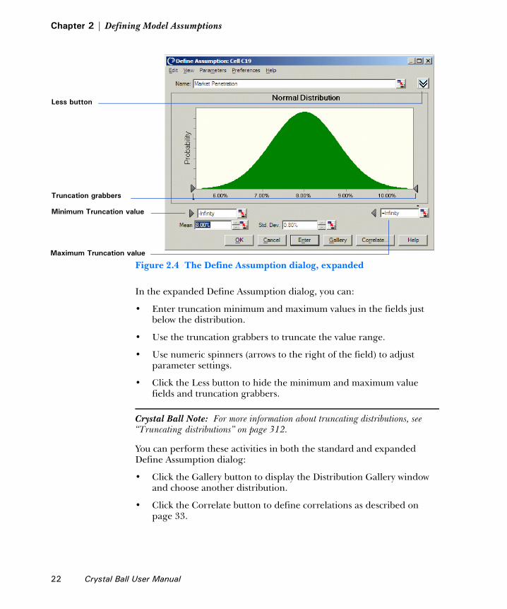
Figure 2.4 The Define Assumption dialog, expanded
In the expanded Define Assumption dialog, you can:
• Enter truncation minimum and maximum values in the fields just below the distribution.
• Use the truncation grabbers to truncate the value range.
• Use numeric spinners (arrows to the right of the field) to adjust parameter settings.
• Click the Less button to hide the minimum and maximum value fields and truncation grabbers.
Crystal Ball Note: For more information about truncating distributions, see “Truncating distributions” on page 312.
You can perform these activities in both the standard and expanded Define Assumption dialog:
• Click the Gallery button to display the Distribution Gallery window and choose another distribution.
• Click the Correlate button to define correlations as described on page 33.
Minimum Truncation value
Maximum Truncation value
Less button
Truncation grabbers
22 Crystal Ball User Manual

Additional assumption features1
• Choose Edit > Add in the menubar to add the currently defined assumption distribution to the Favorites category or a user-defined category in the Distribution Gallery.
• Use other menu commands to copy the chart, paste it into Excel or another application, print data, change the view, use alternate parameters, set assumption and chart preferences, and display help as described in “Additional assumption features” beginning on page 23.
7. When you have finished entering parameters to define the assumption, click Enter.
The distribution changes to reflect the values you entered.
Crystal Ball Note: If you click OK instead of Enter, Crystal Ball accepts the parameters and closes the dialog.
8. Click OK.
If you selected a range of cells, repeat steps 3-8 to define the assumption for each cell.
Additional assumption featuresAs you enter assumption parameters, you can use cell references and alternate parameters. If you have historical data available, you can use Crystal Ball’s distribution fitting feature to help simplify the process of selecting a probability distribution. You can also specify correlations between assumptions or freeze assumptions to exclude them from a simulation.
The following sections discuss advanced features that help you refine assumption definitions and use assumptions more effectively:
• “ Entering cell references and formulas,” below
• “Alternate parameter sets” on page 25
• “Setting assumption preferences” on page 38
• “Fitting distributions to data” on page 27
• “Specifying correlations between assumptions” on page 33
• “Freezing Crystal Ball data cells” on page 88
Crystal Ball User Manual 23
Chapter 2 | Defining Model Assumptions
Entering cell references and formulasIn addition to numeric values, you can enter a reference to a specific cell in a parameter field. Cell references must be preceded by an equals sign (=). Cell references can be either absolute or relative. You can also enter formulas and range names.
If necessary, you can press F4 to change references from relative to absolute or back to relative. This also applies to cell references in fields other than assumption parameters.
Note: All cell references in parameters are treated like absolute references when cutting and pasting Crystal Ball data. Crystal Ball always stores the cell reference in A1 format even if the Excel preference is set to R1C1 format. The global R1C1 format preference is not affected by running Crystal Ball, but the name ranges are, in fact, changed to A1 format since that is the way Crystal Ball stores them.
To show cell references instead of current values when you enter them in parameter fields, choose Parameters > Show Cell References in the Define Assumption dialog.
Dynamic vs. static cell references
Cell references in assumption parameters are dynamic and are updated each time the workbook is recalculated. Dynamic cell referencing gives you more flexibility in setting up models by letting you change an assumption’s distribution during a simulation.
Other types of cell references are static, such as the assumption name field and correlation coefficients. These cell references are calculated once at the beginning of a simulation.
Crystal Ball Note: In previous versions of Crystal Ball, you could choose whether to use static or dynamic cell referencing in parameters. With static referencing, all cell references are resolved at the start of a simulation and then frozen while a simulation is running. If you open a model from a previous version, any static references are converted into dynamic references. If you don’t want parameter values to change when a simulation is running, be sure cell references in parameters do not reference Crystal Ball data cells (assumptions, decision variables, and forecasts) directly or indirectly through formulas.
24 Crystal Ball User Manual

Additional assumption features1
Relative references
Relative references remember the position of a cell relative to the cell containing the assumption. For example, suppose an assumption in cell C6 refers to cell C5. If the assumption in C6 is copied to cell C9, the relative reference to C5 will then refer to the value in cell C8. This lets you easily set up a whole row or column of assumptions, each having similar distributions but slightly different parameters, by performing just a few steps. An absolute reference, on the other hand, always refers back to the originally referenced cell, in this case C5.
Absolute references
To indicate an absolute reference, you must use a dollar sign ($) before the row and the column. For example, to copy the exact contents of cell C5 into an assumption parameter field, you would enter the cell reference =$C$5. This causes the value in cell C5 to be used in the assumption cell parameter field. Later, if you decide to copy and paste this assumption in the worksheet, the cell references in the parameter field will refer to the contents of cell C5.
Range names
You can also enter cell references in the form of range names, such as =cellname. Then, the referenced cell can be located anywhere within a worksheet as long as its name doesn’t change.
Formulas
You can enter Excel formulas to calculate parameter values as long as the formula resolves to the type of data acceptable for that parameter. For example, if a formula returns a string, it wouldn’t be acceptable in a parameter that requires a numeric value, such as Minimum or Maximum.
Alternate parameter setsFor all the continuous probability distributions except uniform, you can define the distributions using percentiles for parameters. This option gives you added flexibility to set up assumptions when only percentile information is available or when specific attributes (such as the mean and standard deviation) of the variable in your model are unknown.
For example, if you are defining a triangular distribution, but are unsure of the absolute minimum and maximum values of the variable, you could instead define the distribution using the 10th and 90th percentiles along with
Crystal Ball User Manual 25

Chapter 2 | Defining Model Assumptions
the likeliest value. This gives you a distribution that has 80%, or four-fifths of the values, occurring between the two specified percentiles, as in Figure 2.5.
To change the parameter sets for the continuous distributions, use the Parameters menu in the menubar of the Define Assumption dialog. The currently selected parameter set has a check mark next to it, as shown on the menu in Figure 2.5.
Figure 2.5 10th and 90th percentiles with Likeliest parameter
In addition to the standard parameter set, each continuous distribution’s Parameters menu has additional pre-defined parameter sets that include various combinations of the standard parameters and percentiles. There is also a Custom command that lets you define your own parameter set.
If you choose Custom in the Parameters menu, you can replace any or all of the standard parameters with any percentile. You will always have the same number of parameters, either standard or alternate, for any given distribution. For example, even if you choose to use custom alternate parameters for a triangular distribution, you will always have three parameters, either minimum, likeliest, and maximum, or, for example, 10th percentile, likeliest, and 99th percentile.
To select a parameter set to use as the default when defining new assumptions of this type, choose Set Default from the Parameters menu.
26 Crystal Ball User Manual

Additional assumption features1
Several special parameter sets are available with the lognormal distribution, including geometric and logarithmic sets. For more information, see the “Equations and Methods” chapter in the online Crystal Ball Reference Manual.
Fitting distributions to dataIf you have historical data available, Crystal Ball’s distribution fitting feature can substantially simplify the process of selecting a probability distribution. Not only is the process simplified, but the resulting distribution more accurately reflects the nature of your data than if the shape and parameters of the distribution were estimated.
How distribution fitting works
In distribution fitting, Crystal Ball automatically matches your data against each continuous probability distribution. A mathematical fit is performed to determine the set of parameters for each distribution that best describe the characteristics of your data. The quality or goodness of each fit is judged using one of several standard goodness-of-fit tests. The distribution with the highest ranking fit is chosen to represent your data.
You can review the distributions sorted in order of their fit tests using the comparison chart. This chart shows the fitted distributions superimposed over your data so you can visually check the quality of the fits. Several chart preferences make it easier to pinpoint discrepancies in the fits. If desired, you can override the highest-ranking probability distribution with another one of your choice.
Crystal Ball Note: Only continuous distributions are considered for distribution fitting. Continuous and discrete distributions are defined on page 249. Distribution fitting can also be used to check the characteristics of a forecast chart. See “Fitting a distribution to a forecast” on page 120 for more information.
Use the Fit Distribution dialog to specify the source of your data, the distributions to be fitted, and the goodness-of-fit test to use. Each goodness-of-fit test is calculated for every distribution, but only the selected test determines how the distributions are ranked.
Crystal Ball Note: Difficulties can occur when distribution fitting is selected for one or more forecasts with large numbers of trials. This is true for Normal
Glossary Term: goodness-of-fit— A set of mathematical tests performed to find the best fit between a standard probability distribution and a data set’s distribution.
Crystal Ball User Manual 27

Chapter 2 | Defining Model Assumptions
as well as Extreme speed. To avoid these difficulties, fitting is disabled for all run modes after 1,000 trials have been run. A final fit is performed when the simulation stops; a progress dialog appears during that fit so you can cancel the fit if necessary.
Using distribution fitting
To use distribution fitting:
1. Select the cell where you want to create an assumption.
It can be blank or contain a simple value, not a formula.
2. Choose Define > Define Assumption.
The Distribution Gallery appears.
3. Click Fit to select the source of the fitted data.
The Fit Distribution dialog appears, as shown in Figure 2.6.
Figure 2.6 Fit Distribution dialog
4. Choose one of the following two options.
• If the historical data is in a worksheet in the active workbook, choose Range, and then enter the data’s cell range.
• If the historical data is in a separate text file, click Text File, and then either enter the path and name of the file or click Browse to search for the file. If you want, you can check Column and enter the number of columns in the text file.
28 Crystal Ball User Manual

Additional assumption features1
Crystal Ball Note: When you use a file as your source of data, each data value in the file must be separated by either a comma, a tab character, a space character, or a list separator defined in Windows’ Regional and Language Options dialog. If actual values in the file contain commas or the designated list separator, those values must be enclosed in quotes. Allowable formats for values are identical to those allowed within the assumption parameter dialog, including date, time, currency, and numbers.
5. Specify which distributions are to be fitted:
• All Continuous fits the data to all of the built-in continuous distributions (these distributions appear as solid shapes on the Distribution Gallery).
• Choose displays another dialog from which you can select a subset of the continuous distributions to include in the fitting.
• The third option selects the continuous distribution that was highlighted on the Distribution Gallery when you clicked the Fit button.
Crystal Ball Note: If you try to fit negative data to a distribution that can only accept positive data, that distribution will not be fitted to the data.
6. Specify how the distributions should be ranked.
In ranking the distributions, you can use any one of three standard goodness-of-fit tests:
• Anderson-Darling. This method closely resembles the Kolmogorov-Smirnov method, except that it weights the differences between the two distributions at their tails greater than at their mid-ranges. This weighting of the tails helps to correct the Kolmogorov-Smirnov method’s tendency to over-emphasize discrepancies in the central region.
• Chi-Square. This test is the oldest and most common of the goodness-of-fit tests. It gauges the general accuracy of the fit. The test breaks down the distribution into areas of equal probability and compares the data points within each area to the number of expected data points. The chi-square test in Crystal Ball does not use the associated p-value the way other statistical tests (e.g., t or F) do.
• Kolmogorov-Smirnov. The result of this test is essentially the largest vertical distance between the two cumulative distributions.
Crystal Ball User Manual 29

Chapter 2 | Defining Model Assumptions
7. Click OK to fit the distributions to your data.
Crystal Ball successively fits the selected distributions to your data. The fitted distributions appear in the Comparison Chart dialog, starting with the highest-ranked distribution down through to the lowest.
You can use the Next and Previous buttons to scroll through the fitted probability distributions. Each probability distribution is shown superimposed over the data, as shown in Figure 2.7.
Figure 2.7 Comparison Chart dialog
8. Use the Comparison Chart dialog to visually compare the quality of the fits or to view the goodness-of-fit statistics.
Use the Comparison Chart features as described below:
• Click the Next and Previous buttons to scroll through the fitted distributions. You can view the quality of each fit graphically and statistically in decreasing order.
• Use the View menu to change the chart view. Choose Goodness of Fit to display results of the different goodness-of-fit tests for each distribution type.
30 Crystal Ball User Manual

Additional assumption features1
Figure 2.8 The Comparison Chart Goodness of Fit view
• Choose Preferences > Chart to change chart features so that similarities or differences are more clearly accentuated.
• Click Cancel to return to the Fit Distribution dialog.
9. To use the currently selected distribution, either the best fit or another of your choice, click Accept.
The Assumption dialog appears with the best-fitting parameters taken from the chosen distribution as shown in Figure 2.9.
You can change the distribution parameters before you click OK.
Crystal Ball User Manual 31
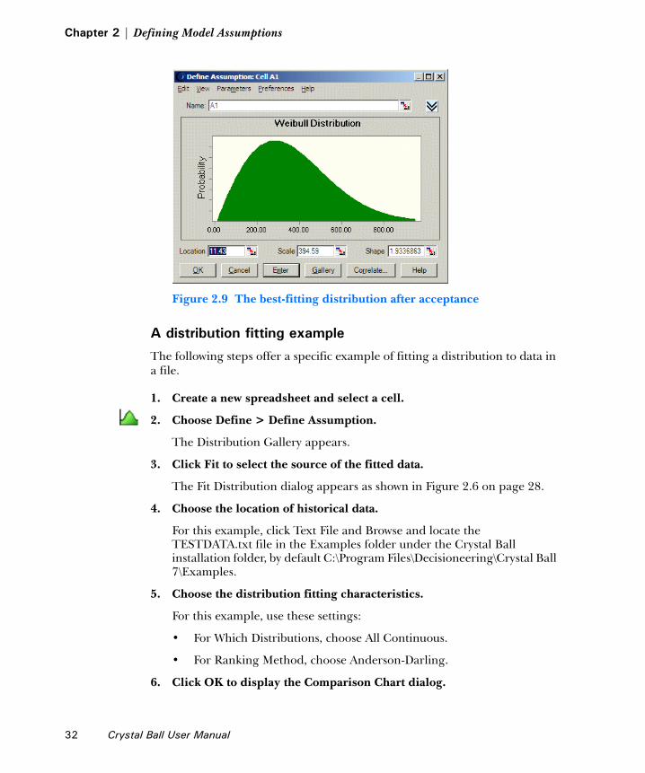
Chapter 2 | Defining Model Assumptions
Figure 2.9 The best-fitting distribution after acceptance
A distribution fitting example
The following steps offer a specific example of fitting a distribution to data in a file.
1. Create a new spreadsheet and select a cell.
2. Choose Define > Define Assumption.
The Distribution Gallery appears.
3. Click Fit to select the source of the fitted data.
The Fit Distribution dialog appears as shown in Figure 2.6 on page 28.
4. Choose the location of historical data.
For this example, click Text File and Browse and locate the TESTDATA.txt file in the Examples folder under the Crystal Ball installation folder, by default C:\Program Files\Decisioneering\Crystal Ball 7\Examples.
5. Choose the distribution fitting characteristics.
For this example, use these settings:
• For Which Distributions, choose All Continuous.
• For Ranking Method, choose Anderson-Darling.
6. Click OK to display the Comparison Chart dialog.
32 Crystal Ball User Manual

Additional assumption features1
For this Test Data example, the Weibull distribution had the best fit of any distribution using the Anderson-Darling fit test. The parameters that were calculated for the Weibull distribution are displayed in Figure 2.8 on page 31.
7. Use the Next and Previous buttons to view comparison charts for the other distributions.
8. Return to Weibull and click Accept.
The Define Assumption dialog appears with the accepted Weibull distribution, as shown in Figure 2.9 on page 32.
Specifying correlations between assumptionsIn Crystal Ball, assumption values are usually calculated independently of each other. Crystal Ball generates random numbers for each assumption without regard to how random numbers are generated for other assumptions.
However, dependencies often do exist between variables in a system being modeled. The Correlated Assumptions feature in Crystal Ball lets you enter correlation coefficients to describe the dependencies between assumptions. Correlation coefficients and correlation in general are explained in the “Statistical Definitions” chapter of the online Crystal Ball Reference Manual.
Crystal Ball Note: Crystal Ball uses Spearman rank correlation to calculate correlation coefficients. For more information on how Crystal Ball calculates Spearman rank correlation coefficients, see “Rank correlation” in the “Statistical Definitions” chapter of the online Crystal Ball Reference Manual.
When defining correlations, the more correlations you define, the greater the possibility that some correlations might be in conflict with each other, preventing Crystal Ball from running a simulation. Conflicts can arise when a group of assumptions are improperly related to each other by large positive and/or large negative correlation coefficients. When this condition occurs, the correlations are said to be “inconsistent.” For more information, see “Correlated assumptions” on page 323.
With Crystal Ball, you use the Define Correlation dialog to specify a correlation coefficient for any pair of assumptions in the same workbook.
To define a correlation coefficient:
1. Select the cell of one of the assumptions you want to correlate — for example, a cell describing the inflation rate.
Crystal Ball User Manual 33
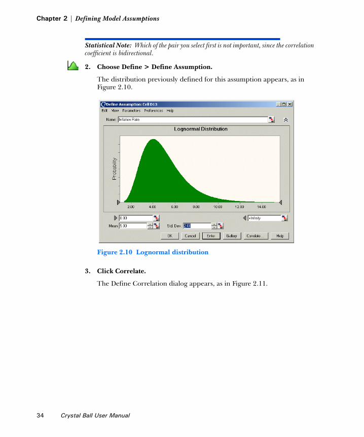
Chapter 2 | Defining Model Assumptions
Statistical Note: Which of the pair you select first is not important, since the correlation coefficient is bidirectional.
2. Choose Define > Define Assumption.
The distribution previously defined for this assumption appears, as in Figure 2.10.
Figure 2.10 Lognormal distribution
3. Click Correlate.
The Define Correlation dialog appears, as in Figure 2.11.
34 Crystal Ball User Manual

Additional assumption features1
Figure 2.11 Define Correlation dialog
4. Click Choose to select the second assumption from the Choose Assumptions dialog.
Crystal Ball Note: You can only correlate assumptions in the same workbook.
The Choose Assumptions dialog provides a list of the names of all the assumptions defined in your workbook.
Figure 2.12 The Choose Assumptions dialog, Tree view
By default, the dialog appears in a hierarchical Tree view. If you prefer, you can click the List icon to change it to List view, shown in the next figure.
Crystal Ball User Manual 35

Chapter 2 | Defining Model Assumptions
Figure 2.13 The Choose Assumptions dialog, List view
5. Choose one or more of the assumption names on the list and click OK.
The cell reference or name of the assumption appears in the list in the left pane of the dialog, as shown in Figure 2.14.
Figure 2.14 Define Correlation dialog with second assumption
After you select the second assumption, the cursor moves to the field below the Choose button, the Coefficient Entry field.
The chosen assumptions appear in the list of correlations. The currently selected assumption also appears immediately next to the Choose button.
Coefficient Entry field
Coefficient slider
Correlation list
Calc button
36 Crystal Ball User Manual

Additional assumption features1
6. Enter a correlation coefficient using one of the following methods:
• Enter a value between -1 and 1(inclusive) in the Coefficient Entry field.
Type the number that you want to use in the field to the left of the slider control. After you type the number, the slider control on the correlation coefficient scale moves to the selected value.
• Choose a cell that contains the correlation coefficient.
Crystal Ball Note: If you choose a cell with values that change during the simulation, it is the initial value of the cell that is used for the coefficient.
• Drag the slider control along the correlation coefficient scale.
The value you select appears in the field to the left of the scale.
• Type the desired correlation coefficient in the Coefficient field in the correlation list.
• Click Calc.
A small dialog appears at the bottom of the first dialog. Enter the range of cells on your spreadsheet that contains the empirical values that Crystal Ball should use to calculate a correlation coefficient.
Enter the range of cells in the standard A1:A2 format, where A designates the column and 1 and 2 designate the first and last cell rows, respectively. For example, if one set of values is in column Q, rows 10 through 15 and the second set of values is in column R, rows 10 through 15, enter the range in the left field as Q10:Q15 and the range in the right field as R10:R15.
Crystal Ball calculates the correlation coefficient, enters it in the field to the left of the correlation coefficient scale, and moves the slider control to the correct position.
Crystal Ball Note: The two cell ranges do not necessarily have to have the same dimensions, but they must contain the same number of value cells and must be in the same workbook. The cell ranges are read in a row-by-row fashion.
Each time you select a new assumption or correlation coefficient, Crystal Ball displays a sample correlation of the correlated assumption values in the chart to the right.
Crystal Ball User Manual 37
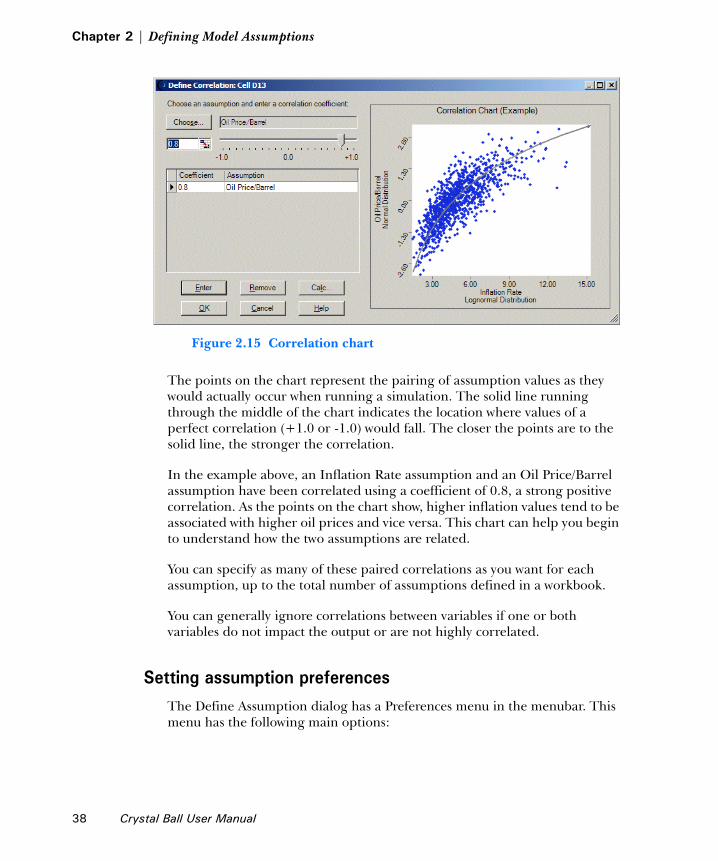
Chapter 2 | Defining Model Assumptions
Figure 2.15 Correlation chart
The points on the chart represent the pairing of assumption values as they would actually occur when running a simulation. The solid line running through the middle of the chart indicates the location where values of a perfect correlation (+1.0 or -1.0) would fall. The closer the points are to the solid line, the stronger the correlation.
In the example above, an Inflation Rate assumption and an Oil Price/Barrel assumption have been correlated using a coefficient of 0.8, a strong positive correlation. As the points on the chart show, higher inflation values tend to be associated with higher oil prices and vice versa. This chart can help you begin to understand how the two assumptions are related.
You can specify as many of these paired correlations as you want for each assumption, up to the total number of assumptions defined in a workbook.
You can generally ignore correlations between variables if one or both variables do not impact the output or are not highly correlated.
Setting assumption preferencesThe Define Assumption dialog has a Preferences menu in the menubar. This menu has the following main options:
38 Crystal Ball User Manual

Additional assumption features1
The Chart Preferences settings are discussed in “Setting chart preferences” beginning on page 128.
If you choose Assumption Preferences, the Assumption Preferences dialog appears as shown in Figure 2.16.
Figure 2.16 The Assumption Preferences dialog
This dialog lets you:
• Choose a view for the assumption chart:
• Probability – shows a graph of all possible values for the assumption variable and the probability of their occurrence.
• Cumulative Probability – shows a graph of the probability that the assumption variable will fall at or below a given value.
• Reverse Cumulative Probability – shows a graph of the probability that the assumption variable will fall at or above a given value.
• Statistics – shows a table of measures of central tendency, variability, minimum and maximum values, and other statistics for the assumption variable.
Table 2.1 Preferences menu, Define Assumptions dialog
Setting Effect
Assumption Preferences Manage window display during simulations
Chart Preferences Determine the appearance of the assumption chart
Crystal Ball User Manual 39

Chapter 2 | Defining Model Assumptions
• Percentiles – shows a table of percentiles and their associated values for the assumption variable.
Note: For examples of each view, see “Changing the distribution view and interpreting statistics” beginning on page 115.
• Determine if and when the assumption chart window appears when a simulation runs.
Crystal Ball Note: To show the generated values in the window, turn on the Store Assumption Values For Sensitivity Analysis run preference. To do so, click the Run Preferences button, then click the Options tab.
For more information about the Assumption Preferences settings, click the Help button in the Assumption Preferences dialog.
You can click Apply To to copy these settings to other assumptions. If necessary, you can click Defaults to restore original default settings. When the settings are complete, click OK.
40 Crystal Ball User Manual

Additional Distribution Gallery features1
Additional Distribution Gallery featuresYou can use the Distribution Gallery to add, manage, and share libraries of distributions. This powerful feature lets work groups modify and share customized distributions over their local networks for collaborative use in custom models. They can also email these to other Crystal Ball users for use with their models.
The following table summarizes how you can use these additional features. For instructions, see the referenced pages.
Table 2.2 Distribution Gallery tasks
How Do I... Command Reference
Display the Distribution Gallery Define > Define Assumption
page 42
Manage distributions
Create new distributions Edit > Add To Gallery (in Define Assumption dialog)
page 45
Copy distributions Edit > Copy page 46
Paste distributions Edit > Paste page 46
Modify distributions Edit > Modify page 47
Modify distribution summaries and descriptions
right-click menu page 48
Delete distributions Edit > Delete page 48
Set up pages for printing Edit > Page Setup page 49
Print distribution information Edit > Print page 49
Manage categories
Create new categories Categories > New page 50
View and edit category properties Categories > Properties page 51
Delete categories Categories > Delete page 51
Rearrange category order Categories > Move Up, Categories > Move Down
page 51
Share categories over networks Categories > Publish, Categories > Subscribe
page 52
Crystal Ball User Manual 41

Chapter 2 | Defining Model Assumptions
Displaying the Distribution GalleryTo display the Distribution Gallery:
1. With Crystal Ball open within Microsoft Excel, click in a cell.
2. Click the Define Assumption tool or choose Define > Define Assumption.
The Distribution Gallery appears, as shown in Figure 2.17.
The Distribution Gallery window
Figure 2.17 The Distribution Gallery window
Use categories shared by others Categories > Subscribe page 53
Send and receive categories page 54
Edi shared categories Categories > Modify page 55
Unpublish shared categories page 55
Change distribution display within categories View menu page 44
View online help Help menu page 5
Table 2.2 Distribution Gallery tasks (Continued)
How Do I... Command Reference
Menubar
Category pane with category folders
Distribution pane
Description pane
42 Crystal Ball User Manual

Additional Distribution Gallery features1
As shown in Figure 2.17, the Distribution Gallery has a menubar, a category pane with folders containing distributions, a distribution pane that displays all distributions in the selected category, and a description pane that describes the selected distribution. The following sections explain each part of the Distribution Gallery.
The Distribution Gallery menubar and buttons
The Distribution Gallery menubar has the menus summarized in Table 2.3.
For more information on how to use these commands, see the references in Table 2.2 on page 41.
The Fit button at the bottom of the Distribution Gallery opens the Crystal Ball distribution fitting feature. This feature can help you select an appropriate distribution for the assumption you are defining. For more information, see “Fitting distributions to data” on page 27.
The Help button displays online help for the currently selected distribution.
Table 2.3 Distribution Gallery menus
Menu Command Summary
Edit Commands that let you copy, paste, modify, and delete distributions. You can copy from any category you are allowed to use but you can only paste, modify, and delete within the Favorites category or new categories you or others have created. You cannot modify or delete distributions in the Basic and All categories; these categories are reserved only for unmodified distributions shipped with Crystal Ball.
Categories Commands that let you create, delete, view and modify properties of, and rearrange category folders in the Category pane. Two additional commands let you share categories with others (Publish) and use categories others have shared (Subscribe).
View Commands that change how distributions appear in the Distribution pane (as Thumbnails, Large Icons, or Small Icons) and hide or show distribution details and descriptions.
Help Commands that display online help for the Distribution Gallery and the selected distribution.
Crystal Ball User Manual 43
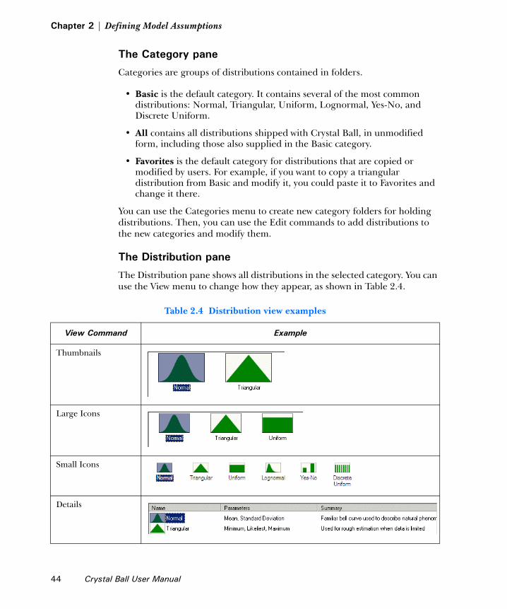
Chapter 2 | Defining Model Assumptions
The Category pane
Categories are groups of distributions contained in folders.
• Basic is the default category. It contains several of the most common distributions: Normal, Triangular, Uniform, Lognormal, Yes-No, and Discrete Uniform.
• All contains all distributions shipped with Crystal Ball, in unmodified form, including those also supplied in the Basic category.
• Favorites is the default category for distributions that are copied or modified by users. For example, if you want to copy a triangular distribution from Basic and modify it, you could paste it to Favorites and change it there.
You can use the Categories menu to create new category folders for holding distributions. Then, you can use the Edit commands to add distributions to the new categories and modify them.
The Distribution pane
The Distribution pane shows all distributions in the selected category. You can use the View menu to change how they appear, as shown in Table 2.4.
Table 2.4 Distribution view examples
View Command Example
Thumbnails
Large Icons
Small Icons
Details
44 Crystal Ball User Manual

Additional Distribution Gallery features1
The Description pane
The Description pane appears at the bottom of the Distribution Gallery and provides a detailed description of the selected distribution.
You can turn off Show Description in the View menu to show more distributions in the Distribution pane.
Managing distributionsWorking with distributions is a key part of defining a model in Crystal Ball. Assumptions are the main source of simulation input and distributions are the core component of assumption definitions.
Several Crystal Ball features help you modify and save distributions for future use and share them with other Crystal Ball users. You can:
• Modify distribution parameters when defining an assumption, and then save the modified distribution directly to the Distribution Gallery for later use.
• Cut and paste default and modified distributions to create custom categories of distributions that you use frequently or use with certain models.
For example, you can copy a small number of frequently used distributions from the All cateogry into Favorites to instantly access your favorite distributions without scrolling through All. Or, you can create a custom category and add them there.
• Modify distribution summaries and descriptions to accompany particular models or reflect parameter changes.
• Delete unwanted distributions from Favorites and custom categories.
• Print distributions for reference and presentation.
Table 2.2 on page 41 summarizes distribution management tasks you can perform in the Distribution Gallery. For instructions, see the referenced pages.
Creating new distributions
You can create new distributions by:
• Copying and renaming a distribution within the Distribution Gallery
• Defining a distribution in the Define Assumption dialog and adding it to the Distribution Gallery
Crystal Ball User Manual 45
Chapter 2 | Defining Model Assumptions
The following sections explain both methods.
Creating distributions by copyingTo create a distribution by copying another distribution, follow the steps in the next section, “Copying and pasting distributions.”
Then, you can rename and modify the new distribution as needed.
Creating distributions by saving assumptionsTo create a distribution by saving an assumption:
1. With Crystal Ball running, click a cell in the spreadsheet.
It can be a value cell where you want to define an assumption or a blank cell.
2. Click the Define Assumption tool or choose Define > Define Assumption.
3. Follow the steps beginning on page 18 to select a distribution and enter parameters.
4. Choose Edit > Add To Gallery in the Define Assumption dialog.
5. The Add To Gallery dialog appears, where you can name the new distribution and select a category for it.
6. Click OK to save the distribution in the selected category.
If you created correlation data, it is not saved although the distribution type and any parameter settings are saved.
Now, the new distribution is available for use just as another other distribution, either supplied with Crystal Ball or user-defined.
Copying and pasting distributions
To copy and paste a distribution within Favorites or another user-defined category or from one category to another:
1. In the Distribution Gallery, click a category in the Category pane.
2. Click a distribution in the Distribution pane.
3. Choose Edit > Copy or right-click and choose Copy from the right-click menu.
4. Click Favorites or another user-defined category in the Category pane.
5. Choose Edit> Paste or right-click and choose Paste from the right-click menu.
46 Crystal Ball User Manual

Additional Distribution Gallery features1
The distribution is pasted into the selected category. If another distribution in that category had the same name, the new distribution appears with the next larger number at the end. For example, if the category already had Normal1, a new normal distribution would be named Normal2.
6. To rename the copied distribution, click its name and wait a moment. The name is highlighted for editing.
7. Type the new name and press Enter.
8. Modify the new distribution as needed.
Crystal Ball Note: To easily copy a distribution from one category to another, select the category with the distribution you want to copy. Then, drag the distribution into the closed category folder where you want to copy it. When you select that category, the copied distribution appears and you can rename it or modify it as described in the next section. However, the distribution you copied remains in its original folder, unchanged.
Modifying distributions
Distributions in the Basic or All categories are read-only and cannot be changed. However, once you have copied a distribution or used it to define an assumption, you can modify it in a number of ways.
To modify a distribution:
1. Create a distribution as described in “Creating new distributions” on page 45 and “Copying and pasting distributions” on page 46.
2. Right-click the user-defined distribution and choose Modify (or click the distribution and choose Edit > Modify in the Distribution Gallery menubar).
3. A prompt appears to remind you that you are modifying a distribution and not defining an assumption.
4. Click OK to display the distribution in a window that looks like the Define Assumption dialog.
5. Modify the distribution as if it were an assumption, following the instructions in “Defining assumptions” beginning on page 18 to modify the distribution.
6. When you are finished, click OK.
The modifications are saved with the distribution in the category and no assumption is created in the spreadsheet.
Crystal Ball User Manual 47

Chapter 2 | Defining Model Assumptions
Modifying distribution summaries and descriptions
You can edit the distribution Summary and Description text for any distribution in Favorites or another user-defined category.
To modify Summary text for a distribution:
1. In the Distribution Gallery, set the View menu to Details.
2. In the Distribution pane, right-click the Summary text you want to edit.
3. In the right-click menu, choose Modify Summary For distribution name.
4. When the Modify Summary dialog appears, enter the new text in the edit field and click OK.
The new text immediately replaces the original Summary text.
To modify Description text for a distribution:
1. Select the distribution in the Distribution Gallery.
2. Be sure View > Show Description is checked.
3. Right-click the text in the Description pane.
4. In the right-click menu, choose Modify Description For distribution name.
5. When the Modify Description dialog appears, edit the description in the edit field and click OK.
The new text immediately replaces the original description.
Crystal Ball Note: Alternately, you can just select the description text to modify and edit it. Be careful to avoid modifying descriptions accidentally.
Deleting distributions
You can delete a distribution in the Favorites category or other user-defined category. However, the original distribution of that type remains in Basic or All.
To delete a distribution, choose Edit > Delete in the Distribution Gallery menubar, or right-click the distribution and choose Delete.
48 Crystal Ball User Manual
Additional Distribution Gallery features1
Setting up distributions for printing
To select paper, print orientation, and margins before printing:
1. Double-click a distribution in the Distribution Gallery to display it in the Define Assumption dialog.
2. Choose Edit > Page Setup in the Define Assumption menubar.
3. Set paper size and source, orientation, and margins.
4. Click OK to accept the settings.
Printing distribution information
To print a distribution:
1. Double-click a distribution in the Distribution Gallery to display it in the Define Assumption dialog.
2. Choose Edit > Print in the Define Assumption menubar.
3. Confirm the printer and other settings.
4. Click OK to print the distribution.
Printed information includes the chart with current parameter settings. The distribution name and parameters appear in a box beneath the graphic.
Crystal Ball Note: You can preview before printing. In step 2, choose Edit > Print Preview before you choose Edit > Print.
Managing categoriesYou can use distribution categories to organize distributions and share them with other users in your organization. For example, you can:
• Create a category to hold a few distributions you use most often.
• Create a category to hold all distributions related to a certain model or series of models.
• Create a category with distributions you want to share with other users.
• Delete categories you no longer need.
• Rearrange category order within the Distribution Gallery.
• Share, or publish, categories with other users over networks.
Crystal Ball User Manual 49

Chapter 2 | Defining Model Assumptions
• Use categories that others have published.
• Unpublish categories that are no longer needed.
Table 2.2 on page 41 summarizes category management tasks you can perform in the Distribution Gallery. For instructions, see the referenced pages.
Creating new categories
You can create a category of distributions to help with model development or to share with other users.
To create a category:
1. Choose Categories > New.
The New Category dialog box appears, as shown in Figure 2.18.
Figure 2.18 The New Category dialog
2. Enter the name of your category. Optionally, you can enter a description, your name, and a version number (helpful for shared categories).
Note: If you enter an ampersand (&) before a letter in the category name, that letter becomes a shortcut key. You can then use it to select the category from the keyboard by holding down the Alt key and pressing the shortcut key. Shortcut keys appear underlined when you press the Alt key. The new category should use a different shortcut key from other categories.
3. Click OK.
The new folder appears in the Category pane and the category can be selected and used like Favorites or any other user-defined category.
50 Crystal Ball User Manual

Additional Distribution Gallery features1
Viewing and editing category properties
Category properties include the information entered in the New Category dialog when a category is created. You can view properties for any category, but you can only edit properties for user-defined categories.
To view or edit properties:
1. Click a category in the Category pane.
2. Choose Categories > Properties.
The Category Properties dialog appears.
3. You can edit the information in any field that appears white. Read-only fields are gray.
4. When you have finished viewing or editing category properties, click OK.
The Category Properties dialog closes and any property changes are saved.
Deleting categories
You can delete user-defined categories and all the distributions within them, but be careful not to delete a distribution you will need to use later.
To delete a category:
1. Select the category in the Category pane.
2. Choose Categories > Delete.
A confirmation message appears.
3. When you click OK, the category and all its distributions are immediately deleted.
Crystal Ball Note: Original built-in distributions shipped with Crystal Ball are never deleted; only copies can be deleted.
Rearranging category order
Changing the order of folders in the Category pane can be helpful if you want to arrange categories in alphabetical order or put frequently used categories near the top.
Crystal Ball User Manual 51

Chapter 2 | Defining Model Assumptions
To move a category folder:
1. Select the folder you want to move in the Category pane.
2. Choose Categories > Move Up or Categories > Move Down.
The folder moves up or down one position each time you choose the menu command.
3. Continue moving folders up and down until they are arranged as preferred.
Sharing categories over networks
The ability to publish and subscribe to categories is very powerful. You can create large numbers of specific distributions, add them to a category, and then publish it on the network for other users in your organization. Likewise, you can easily subscribe to categories published by others. You can also email categories to others and use categories sent to you.
To publish a category to a shared folder on your computer or to a location on a network:
1. Select a category in the Distribution Gallery.
2. Choose Categories > Publish.
The Browse For Folder dialog appears, as shown in Figure 2.19.
Figure 2.19 The Browse For Folder dialog
3. Browse to locate the folder where you want to place the category. You can click + to expand a folder and view its subfolders. If you need to create a new folder, select the folder that should include the new folder.
52 Crystal Ball User Manual

Additional Distribution Gallery features1
The new folder appears and you can rename it. For example, if you want to create a folder under My Documents, select My Documents. Then, when you click New Folder, the new folder appears under My Documents at the same level as My Pictures.
4. Click OK.
The dialog closes and a copy of your category is saved there.
Using shared categories
If other users have published categories in a shared folder on their computers or the network, you can access them for use with the Distribution Gallery. This is called subscribing to categories.
To subscribe to a category, learn its name and location, then:
1. Open the Distribution Gallery and choose Categories > Subscribe.
2. The Subscribe To A Category dialog appears, as shown in Figure 2.20.
Figure 2.20 The Subscribe To A Category dialog
3. Click Add.
4. The Browse For Folder dialog appears, as shown in Figure 2.19 on page 52. Locate the target folder and click OK to add the new path to the Subscribe To A Category dialog box.
5. Click OK to load all categories in the listed paths and close the Subscribe To A Category dialog box.
All loaded categories are available for use as if they were on your local computer.
Crystal Ball User Manual 53

Chapter 2 | Defining Model Assumptions
Crystal Ball Note: Shared categories can be used like local categories in most ways. However, they cannot be modified unless they also exist in a folder on your local computer. If several users copy a published category locally and then modify it, they can publish their own versions and overwrite each others’ changes. If you are publishing a category, you might want to make the shared folder read-only to avoid this problem.
To edit or delete a path, or rearrange the path order:
1. Open the Subscribe To A Category dialog as described in step 2 above.
2. Select the path to a target category.
3. Click an action button: Edit, Delete, Move Up, or Move Down.
4. When you are finished, click OK.
If you delete a path to a subscribed category, that category disappears from the Category pane of the Distribution Gallery. You can resubscribe to it at any time to use it again.
Sharing categories through email
You can use email to share a user-defined category with a Crystal Ball user who is not on your network.
To share categories using email:
1. Create and address an email message.
2. Use the file attachment command and browse to the category folder on your machine.
By default, this is C:\Documents and Settings\your username\Application Data\Decisioneering\Crystal Ball\7.x\Store.
3. Select the user-defined category to send.
Crystal Ball category files have this format: CBCategory_name.cbc. For example, the Favorites category appears as CBCategory_Favorites.cbc.
4. Send the email.
To use a category received in an email:
1. Open the email.
2. Save the attachment in the Crystal Ball category folder, by default C:\Documents and Settings\your username\Application Data\Decisioneering\Crystal Ball\7.x\Store.
54 Crystal Ball User Manual

Additional Distribution Gallery features1
The next time you start Crystal Ball, the new category appears in the Category pane of the Distribution Gallery.
Alternately, you can save the attachment in another folder, then follow the steps in “Using shared categories” on page 53 to subscribe to it.
Editing shared categories
If you have published a user-defined category and want to change it:
1. Make the changes in your Distribution Gallery.
2. Follow the steps in “Sharing categories over networks” on page 52 to publish the category to the same place.
3. When you are prompted to overwrite the existing file, click OK.
This publishes the modified category. Now, the next time a subscriber loads Crystal Ball, the modified category appears in the Distribution Gallery.
Unpublishing shared categories
If you have published a user-defined category and want to remove it from publication, or “unpublish” it:
1. Use My Computer or Windows Explorer to browse to the folder where the category was published.
The category file appears as CBCategory_name.cbc. For example, the Favorites category would appear as CBCategory_Favorites.cbc.
2. Select the category file and delete it.
Now, the next time a subscriber loads Crystal Ball, the deleted category will not appear in the Distribution Gallery. Existing assumptions based on distributions from that category will still work but those distributions won’t be available for creating new assumptions.
A note about modifying shared categories
If a shared category is moved, deleted, or otherwise modified, subscribers to that category won’t notice the changes until they close Crystal Ball and open it again. It is wise to notify subscribers when a change of that type occurs so they can start a new Crystal Ball session and refresh their view of the Distribution Gallery.
Crystal Ball User Manual 55

Chapter 2 | Defining Model Assumptions
56 Crystal Ball User Manual
Chapter 3Defining Other Model Elements
In this chapter• Defining decision variable cells
• Defining forecasts
• Working with Crystal Ball data
• Setting cell preferences
• Saving and restoring your models
Chapter 2 describes how to start building a spreadsheet model by defining assumption cells. This chapter provides step-by-step instructions for completing models in Crystal Ball so you can run simulations against them. As you work through these instructions, you will learn to define decision variable cells and forecasts and how to cut, copy, and paste Crystal Ball data.
After you complete this chapter, read Chapter 4 for information on setting run preferences and running simulations.
Crystal Ball User Manual 57

Chapter 3 | Defining Other Model Elements
Defining decision variable cells and forecast cellsChapter 2 describes how to define assumption cells and use the Distribution Gallery. This chapter describes how to define decision variable cells and forecast cells and perform other tasks needed to complete a model definition.
Defining decision variable cellsDecision variables are not required for simulation models, but they can be useful when comparing and optimizing alternate scenarios. Several of the Crystal Ball tools discussed in Chapter 8, “Crystal Ball Tools,” use and benefit from decision variables. Decision variables are the variables that you can control, such as rent to charge or the amount of money to invest.
OptQuest Note: You also use decision variables with OptQuest, available with Crystal Ball Professional and Premium Editions.
To define a decision variable cell:
1. Select a cell or range of cells.
Select value cells or blank cells only. You cannot define a decision on a formula or non-numeric cell.
2. Select Define > Define Decision.
The Define Decision Variable dialog appears.
Figure 3.1 Define Decision Variable dialog
58 Crystal Ball User Manual
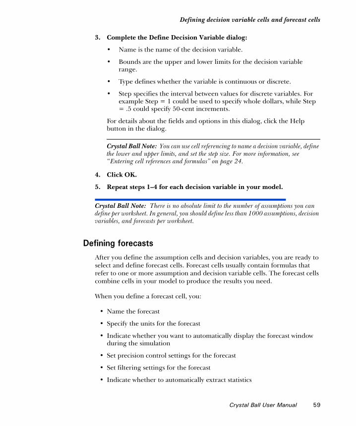
Defining decision variable cells and forecast cells1
3. Complete the Define Decision Variable dialog:
• Name is the name of the decision variable.
• Bounds are the upper and lower limits for the decision variable range.
• Type defines whether the variable is continuous or discrete.
• Step specifies the interval between values for discrete variables. For example Step = 1 could be used to specify whole dollars, while Step = .5 could specify 50-cent increments.
For details about the fields and options in this dialog, click the Help button in the dialog.
Crystal Ball Note: You can use cell referencing to name a decision variable, define the lower and upper limits, and set the step size. For more information, see “ Entering cell references and formulas” on page 24.
4. Click OK.
5. Repeat steps 1–4 for each decision variable in your model.
Crystal Ball Note: There is no absolute limit to the number of assumptions you can define per worksheet. In general, you should define less than 1000 assumptions, decision variables, and forecasts per worksheet.
Defining forecastsAfter you define the assumption cells and decision variables, you are ready to select and define forecast cells. Forecast cells usually contain formulas that refer to one or more assumption and decision variable cells. The forecast cells combine cells in your model to produce the results you need.
When you define a forecast cell, you:
• Name the forecast
• Specify the units for the forecast
• Indicate whether you want to automatically display the forecast window during the simulation
• Set precision control settings for the forecast
• Set filtering settings for the forecast
• Indicate whether to automatically extract statistics
Crystal Ball User Manual 59

Chapter 3 | Defining Other Model Elements
Crystal Ball Note: If you have activated the Crystal Ball process capability features, you can also enter a lower specification limit (LSL), an upper specification limit (USL), and a Target value. For more information, see “Setting specification limits and targets” on page 343.
To define forecast cells:
1. Select a formula cell or a range of formula cells.
2. Select Define > Define Forecast.
The Define Forecast dialog appears.
Figure 3.2 Define Forecast dialog
Crystal Ball Note: If you have activated Crystal Ball’s process capability features, additional fields appear. These are described in “Setting specification limits and targets” on page 343.
3. Complete the Define Forecast dialog:
• Name is the name of the forecast.
• Units is the name of the units that will appear at the bottom of the forecast chart, such as Millions.
For details about the fields and options in this dialog, click the Help button in the dialog.
4. To set additional forecast preferences, click the More button to expand the Define Forecast dialog.
The expanded Define Forecast dialog has four tabs of additional options and fields, listed in “Setting forecast preferences” on page 61.
5. Click OK.
6. Repeat steps 1–4 for each forecast in your model.
60 Crystal Ball User Manual

Defining decision variable cells and forecast cells1
Crystal Ball Note: There is no absolute limit to the number of assumptions you can define per worksheet. In general, you should define less than 1000 assumptions, decision variables, and forecasts per worksheet.
The Expanded Define Forecast dialog also has the Defaults button. Clicking on Defaults restores the original default settings in place of any new settings you have made. You can also click Apply To to use the settings in other charts and worksheets. For more information, click the Help button in the Apply To dialog.
Setting forecast preferences
The forecast preference settings appear when you click the More button in the Define Forecast dialog box. You can also display them by choosing Preferences > Forecast in a forecast chart menubar. The tabs in this dialog control several important aspects of Crystal Ball:
• “Forecast Window preferences” on page 62 — window display and distribution fitting for the forecast
• “Precision preferences” on page 64 — precision control settings
• “Filter preferences” on page 66 — value filtering, which discards values inside or outside a range for the current forecast
• “Auto Extract preferences” on page 68 — automatic data extraction to Excel when a simulation stops.
Crystal Ball Note: For more information on setting the Precision Control option and settings, see “Precision control” on page 318. See “Confidence intervals” in the “Statistical Definitions” chapter of the online Crystal Ball Reference Manual for more information about how absolute and relative precision relate to the confidence interval.
When you expand the Define Forecast dialog or open the Forecast Preferences dialog, the Forecast Window tab appears by default, as shown in Figure 3.3.
Crystal Ball User Manual 61

Chapter 3 | Defining Other Model Elements
Forecast Window preferences
Figure 3.3 Forecast Window tab, forecast preferences
This tab manages window display and distribution fitting for the forecast.
You can choose among the settings listed in Table 3.1. Then, click OK to apply settings on the current tab to the active forecast. Or, you can click Apply To to apply settings on the active tab to the active worksheet, the active workbook, or all workbooks. For more information, click Apply To and then click Help in the Apply To dialog.
At any time, you can click Defaults to restore the original default settings on the active tab in the dialog.
62 Crystal Ball User Manual

Defining decision variable cells and forecast cells1
Table 3.1 Forecast Window tab, forecast preferences
Setting Effect
View Sets the forecast window’s display type. For more information on the View settings, see “Changing the distribution view and interpreting statistics” on page 115.
Frequency Shows the number or frequency of values occurring in a given interval (bin). This is the default view.
Cumulative Frequency
Shows the number or proportion (percentage) of values less than or equal to a given amount.
Reverse Cumulative Frequency
Shows the number or proportion (percentage) of values greater than or equal to a given amount.
Statistics Shows a set of descriptive statistics for the forecast values.
Percentiles Shows percentile information, in 10% increments.
Goodness Of Fit If distribution fitting is selected for the forecast chart, shows goodness-of-fit statistics for the selected distribution and ranking method.
Capability Metrics
If process capability metrics are set for display, shows a table of process capability (quality) statistics for the simulation. See “Viewing capability metrics” on page 344 for more information.
Split View When selected, shows all selected views simultaneously. For details, see “Using Split View” on page 122.
Window Sets whether to display the forecast window automatically while the simulation is running or when the simulation is stopped.
You can display one or more forecasts while the simulation is running. If you decide not to display the forecast, the simulation continues to run. You can override this option and close all the forecast windows using the Suppress Forecast Windows option in the Run Preferences dialog. For more information, see “Setting run preferences” on page 80.
While Running Simulation
Displays the forecast window automatically during simulations. This slows down the simulation.
When Simulation Stops
Displays the forecast window automatically after the simulation stops. This is faster than displaying the window during simulations.
Fit Distribution
Fits a continuous probability distribution to the forecast. After selecting this checkbox in this group, you can click Fit Options to select the distribution and goodness-of-fit tests you want.
Crystal Ball User Manual 63
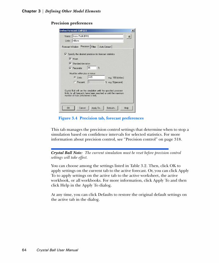
Chapter 3 | Defining Other Model Elements
Precision preferences
Figure 3.4 Precision tab, forecast preferences
This tab manages the precision control settings that determine when to stop a simulation based on confidence intervals for selected statistics. For more information about precision control, see “Precision control” on page 318.
Crystal Ball Note: The current simulation must be reset before precision control settings will take effect.
You can choose among the settings listed in Table 3.2. Then, click OK to apply settings on the current tab to the active forecast. Or, you can click Apply To to apply settings on the active tab to the active worksheet, the active workbook, or all workbooks. For more information, click Apply To and then click Help in the Apply To dialog.
At any time, you can click Defaults to restore the original default settings on the active tab in the dialog.
64 Crystal Ball User Manual
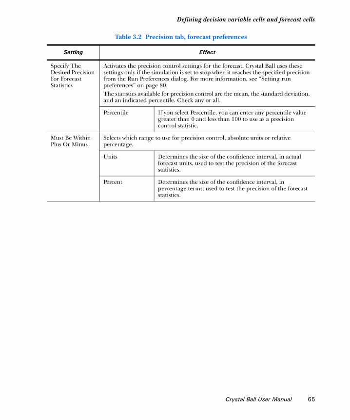
Defining decision variable cells and forecast cells1
Table 3.2 Precision tab, forecast preferences
Setting Effect
Specify The Desired Precision For Forecast Statistics
Activates the precision control settings for the forecast. Crystal Ball uses these settings only if the simulation is set to stop when it reaches the specified precision from the Run Preferences dialog. For more information, see “Setting run preferences” on page 80.The statistics available for precision control are the mean, the standard deviation, and an indicated percentile. Check any or all.
Percentile If you select Percentile, you can enter any percentile value greater than 0 and less than 100 to use as a precision control statistic.
Must Be Within Plus Or Minus
Selects which range to use for precision control, absolute units or relative percentage.
Units Determines the size of the confidence interval, in actual forecast units, used to test the precision of the forecast statistics.
Percent Determines the size of the confidence interval, in percentage terms, used to test the precision of the forecast statistics.
Crystal Ball User Manual 65

Chapter 3 | Defining Other Model Elements
Filter preferences
Figure 3.5 Filter tab, forecast preferences
This tab lets you discard values inside or outside a range for the current forecast or globally for all forecasts in a model. The values are not permanently deleted, only discarded for the purposes of your current analysis.
You can choose among the settings listed in Table 3.3. Then, click OK to apply settings on the current tab to the active forecast. Or, you can click Apply To to apply settings on the active tab to the active worksheet, the active workbook, or all workbooks. For more information, click Apply To and then setting without using Apply To. For more information, see Table 3.3 on page 67.
At any time, you can click Defaults to restore the original default settings on the active tab in the dialog.
66 Crystal Ball User Manual
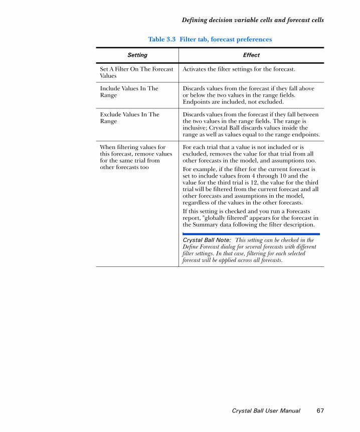
Defining decision variable cells and forecast cells1
Table 3.3 Filter tab, forecast preferences
Setting Effect
Set A Filter On The Forecast Values
Activates the filter settings for the forecast.
Include Values In The Range
Discards values from the forecast if they fall above or below the two values in the range fields. Endpoints are included, not excluded.
Exclude Values In The Range
Discards values from the forecast if they fall between the two values in the range fields. The range is inclusive; Crystal Ball discards values inside the range as well as values equal to the range endpoints.
When filtering values for this forecast, remove values for the same trial from other forecasts too
For each trial that a value is not included or is excluded, removes the value for that trial from all other forecasts in the model, and assumptions too.For example, if the filter for the current forecast is set to include values from 4 through 10 and the value for the third trial is 12, the value for the third trial will be filtered from the current forecast and all other forecasts and assumptions in the model, regardless of the values in the other forecasts.If this setting is checked and you run a Forecasts report, "globally filtered" appears for the forecast in the Summary data following the filter description.
Crystal Ball Note: This setting can be checked in the Define Forecast dialog for several forecasts with different filter settings. In that case, filtering for each selected forecast will be applied across all forecasts.
Crystal Ball User Manual 67

Chapter 3 | Defining Other Model Elements
Auto Extract preferences
Figure 3.6 Auto Extract tab, forecast preferences
This tab lets you specify which statistics to extract automatically to Excel after the simulation stops.
Crystal Ball Note: The Auto Extract settings create tables of unformatted statistics primarily for use in other analyses. To extract formatted data, see “Extracting data” on page 190.
You can choose among the settings listed in Table 3.4. Then, click OK to apply settings on the current tab to the active forecast. Or, you can click Apply To to apply settings on the active tab to the active worksheet, the active workbook, or all workbooks. For more information, click Apply To and then click Help in the Apply To dialog.
At any time, you can click Defaults to restore the original default settings on the active tab in the dialog.
68 Crystal Ball User Manual

Working with Crystal Ball data1
Working with Crystal Ball dataYou can use special commands to copy, paste, and clear Crystal Ball cell definitions from cells. These are different from similar Excel commands and must be used to copy Crystal Ball cell definitions (data). Other Crystal Ball commands let you select and review your data. The following sections describe these data commands.
Editing Crystal Ball dataCrystal Ball provides edit commands to let you copy, paste, or clear assumptions, decision variables, or forecasts from cells. This feature lets you set up an entire row or column of assumptions, decision variables, or forecasts with just a few steps.
If you select a range of cells with more than one kind of Crystal Ball data — for example, an assumption and a forecast — Crystal Ball prompts for which data type you want to copy or clear.
If you want to copy Crystal Ball cell definitions, use only the Crystal Ball Copy Data, Paste Data, or Clear Data commands. Using the Excel copy and paste commands only copies the cell value and attributes, including cell color or pattern.
Table 3.4 Auto Extract tab, forecast preferences
Setting Effect
Extract Forecast Statistics Automatically...
Activates the auto-extract feature.
listbox at the left The list of statistics you can extract. Check the statistics you want, then use the up and down arrows to rearrange their order, if you want.
Starting Cell The first cell on the forecast’s worksheet where the statistics will be copied. Be sure no data entries appear to the right of this cell and below it because data could be overwritten without warning.
Formatting Whether to include labels on the extracted statistics and use Excel’s AutoFormat for the cells.
Direction Whether the extraction proceeds vertically (downward) or horizontally (to the right) on the worksheet.
Crystal Ball User Manual 69

Chapter 3 | Defining Other Model Elements
Excel Note: The Excel commands do not copy the Crystal Ball data, even though they might appear to since the cell colors are copied. To copy Excel data and Crystal Ball data, you must use the Excel edit commands and then use the Crystal Ball edit commands to copy the Crystal Ball data.
Copying Crystal Ball data
To copy Crystal Ball assumptions, decision variables, or forecasts from one area of the spreadsheet to another area in the same workbook or a different workbook:
1. Select a cell or a range of cells that contains the Crystal Ball data you want to copy.
2. Select Define > Copy Data.
If you select a range of cells with more than one kind of Crystal Ball data — for example, an assumption and a forecast — Crystal Ball prompts for which data type you want to copy.
3. Check the type or types to copy and click OK.
Crystal Ball “remembers” the description of the selected cell range.
Pasting Crystal Ball data
To paste Crystal Ball data:
1. Select a cell or a range of cells that you want to paste into.
Usually, you will want it to be at least as large as the range you copied. It should contain cells with values if you are pasting assumptions or decision variables (unless the range is all blank; see note below) and cells with formulas if you are pasting forecasts. It can be on a different worksheet in the same or a different workbook.
Crystal Ball Note: If you are pasting assumptions and/or decision variables into a completely blank range of cells, Crystal Ball pastes them along with the underlying cell value from each copied cell. This does not work for forecasts, which must be pastsed into a cell with a formula, or if there is already data in any cell within the range.
2. Choose Define > Paste Data.
Crystal Ball pastes all selected data types (assumptions, decision variables, and forecasts) from the copied range into the range selected in step 1. Any existing Crystal Ball data in the range selected for pasting will be overwritten.
70 Crystal Ball User Manual

Working with Crystal Ball data1
Crystal Ball Note: If there are more Crystal Ball data cells in the copied range than there are appropriate cells in the range selected for pasting, as many cells as possible of the appropriate type will be pasted; the remaining cells are ignored. If there are more cells in the range selected for pasting than in the range that was copied, the copied cells are reused, starting with the first one in the list.
Note that when you copy a range, Crystal Ball “remembers” the area covered by the range but not the contents of the range. When you paste, you paste all Crystal Ball data of the copied type or types currently within that range regardless of what was there when you copied it. For example, suppose you have two assumption cells in a range. You use the Crystal Ball Copy Data command to copy all types of data cells in the range. Then, you delete one assumption, modify the other, and add a forecast definition to another cell within the range. When you use the Crystal Ball Paste Data command, you then paste the current contents of the range — the remaining modified assumption cell and the new forecast cell.
For best results, use the Paste Data command immediately after the Copy Data command. You are probably already familiar with this from using Excel; if you copy in Excel and then do anything else but select a range for pasting, the copied area is unselected and you must select it again before continuing.
Clearing Crystal Ball data
To clear Crystal Ball data:
1. Select a cell or a range of cells that contains the Crystal Ball data you want to clear.
2. Select Define > Clear Data.
If you select a range of cells with more than one kind of Crystal Ball data — for example, an assumption and a forecast — Crystal Ball prompts for which data type you want to clear.
3. Check the type or types to clear and click OK.
Crystal Ball clears the selected Crystal Ball data type (assumptions, decision variables, and forecast definitions) from each cell.
To clear all of one type of Crystal Ball data from all cells in the active worksheet:
1. Select either:
• Define > Select All Assumptions
• Define > Select All Decisions
Crystal Ball User Manual 71

Chapter 3 | Defining Other Model Elements
• Define > Select All Forecasts
2. Select Define > Clear Data.
Crystal Ball clears the Crystal Ball data from all the selected cells in the active worksheet.
Excel Note: Edit > Clear > All also clears all Crystal Ball data from selected cells.
Selecting and reviewing your dataAfter you define assumptions, decision variables, and forecast cells and return to the spreadsheet, you might want to check the cell definitions to make sure you have defined them as you intended. With Crystal Ball, you can select all the assumption, forecast, and decision variable cells and check their corresponding dialogs in sequence.
Reviewing assumption cells
To review all assumption cells:
1. Select Define > Select All Assumptions.
Crystal Ball selects each cell defined as an assumption.
2. Select Define > Define Assumption.
The distribution dialog for the first assumption cell appears.
3. Change the assumption parameters (optional).
4. Click OK.
If you have more than one assumption cell, each assumption appears in turn. Repeat steps 3 and 4 to check the assumptions for each cell.
Reviewing decision variable cells
To review all decision variable cells:
1. Select Define > Select All Decisions.
Crystal Ball selects each cell defined as a decision variable.
2. Select Define > Define Decision.
The Define Decision Variable dialog for the first decision variable cell appears.
3. Change the decision variable parameters (optional).
72 Crystal Ball User Manual

Working with Crystal Ball data1
4. Click OK.
If you have more than one decision variable cell, each decision variable appears in turn. Repeat steps 3 and 4 to check the decision variables for each cell.
Reviewing forecast cells
To review all forecast cells:
1. Select Define > Select All Forecasts.
Crystal Ball selects each cell defined as a forecast.
2. Select Define > Define Forecast.
The forecast dialog for the first forecast cell appears.
3. Change the forecast definition (optional).
4. Click OK.
If you have selected more than one forecast cell, each forecast appears in turn. Repeat steps 3 and 4 to check the forecast for each cell.
Reviewing selected cells
To review Crystal Ball data cells on any open workbook:
1. Select Define > Select.
The Select dialog appears, as shown in Figure 3.7.
Figure 3.7 Select dialog, Tree view
Forecast button
Decision Variable button
Assumption button
Crystal Ball User Manual 73

Chapter 3 | Defining Other Model Elements
By default, the dialog appears in hierarchical Tree view. All the assumptions are listed first, then all the decision variables, and finally all the forecasts.
You can click the Assumption, Decision Variable, and Forecast buttons to show and hide assumptions, decision variables, and forecasts, respectively. If you prefer to view available cells in list format (shown in Figure 3.8), click the List button.
Figure 3.8 Select dialog, List view
2. Check the cells you want to select.
3. Click OK to highlight all the selected cells so you can change their preferences or perform other actions on them.
You can use the Select dialog to select cells on more than one worksheet but you need to activate each worksheet in turn to review and, if desired, apply a command to all the selected cells.
Setting cell preferencesCrystal Ball lets you change the appearance of assumption, forecast, and decision variable cells so you can quickly identify them on your spreadsheets. You can set Crystal Ball to change the appearance of these cells as you define them, or you can change the appearance of predefined cells.
To set cell preferences,
1. Choose Define > Cell Preferences.
The Cell Preferences dialog appears, as shown in Figure 3.9.
74 Crystal Ball User Manual

Setting cell preferences1
Figure 3.9 The Cell Preferences dialog
2. Click the tab for the kind of cell to format: Assumption, Decision Variables, or Forecast.
3. Make appropriate settings for the chosen cell type:
• Color — Changes the color of each Crystal Ball data cell of the type modified by the selected tab.
• Pattern — Changes the pattern of each Crystal Ball data cell of the type modified by the selected tab.
• Add Comment To Cell — Adds an Excel comment that provides more information about the Crystal Ball data within each cell.
Crystal Ball Note: Crystal Ball only updates cell comments when you define or redefine an assumption, decision variable, or forecast.
• Set Cell Value To... — Changes assumption cell values to the selected value (Mean or Median) when no simulation is running.
• Set To Range Midpoint — Changes decision variable cell values to the selected value (range Midpoint, Minimum, or Maximum) when no simulation is running.
For more information, click the Help button in the dialog.
4. Click Apply To.
The Apply To dialog appears, as shown in Figure 3.10.
Crystal Ball User Manual 75

Chapter 3 | Defining Other Model Elements
Figure 3.10 The Apply To dialog for cell preferences
5. Choose whether to apply settings from only the current tab or all tabs in the Cell Preferences dialog.
6. Choose whether to apply the settings to all cell preferences of the chosen type(s) on the current Excel worksheet, all worksheets in the current workbook, or all open workbooks and any new workbooks to be created later.
Crystal Ball Note: The default is All Workbooks (Open And New).
7. Click OK to close the Apply To dialog and apply the settings to the chosen cell types and worksheets.
Crystal Ball Note: Unlike some other preferences, cell preferences must be applied to all cells of the selected type(s) on the chosen worksheet(s) or workbook(s). If necessary, you can click the Defaults button before choosing Apply To to clear your cell preference settings and restore the original defaults.
Saving and restoring your modelsThe distributions you specified for each assumption cell, the settings you specified for each forecast cell, and the range information for each decision variable cell are saved with their spreadsheet through the Excel save process. When you open the spreadsheet again, Crystal Ball retains your assumption, forecast, and decision variable cells.
Crystal Ball Note: When you run simulations, as described in the next chapter, you can also save and restore simulation results in a separate file for future display and analysis. For details, see page 97.
76 Crystal Ball User Manual

Chapter 4Running Simulations
In this chapter• About Crystal Ball simulations
• Setting run preferences
• Running simulations
• Managing chart windows
• Saving and restoring simulation results
• Running user-defined macros
Chapters 2 and 3 describe how to define a spreadsheet model in Crystal Ball. This chapter provides step-by-step instructions for setting run preferences and running a simulation in Crystal Ball. After you complete this chapter, read Chapter 5 for information about analyzing simulation results.
Crystal Ball User Manual 77

Chapter 4 | Running Simulations
About Crystal Ball simulationsSpreadsheet risk analysis uses both a spreadsheet model and simulation to analyze the effect of varying inputs on outputs of the modeled system.
After you define assumption, forecast, and decision variable cells in your spreadsheet model, you are ready to run the simulation. Crystal Ball uses a technique called Monte Carlo simulation to forecast the entire range of results most likely to occur in the situation you have defined in your spreadsheet model. This technique involves generating random numbers for the assumption variables. For more information on Monte Carlo simulation, see page 11.
While the simulation is running, Crystal Ball displays these assumption results in a forecast chart that shows the entire range of possible outcomes. Crystal Ball provides descriptive statistics for any forecast, which summarize the results numerically. The “Statistical Definitions” chapter of the online Crystal Ball Reference Manual discusses descriptive statistics.
How Crystal Ball uses Monte Carlo simulationMost real-world problems involving elements of uncertainty are too complex to solve analytically. There are simply too many combinations of input values to calculate every possible result. Monte Carlo simulation is an efficient technique that requires only a random number table or a random number generator on a computer.
Crystal Ball implements Monte Carlo simulation in a repetitive three-step process. For each trial of a simulation, Crystal Ball repeats the following three steps:
1. For every assumption cell, Crystal Ball generates a random number according to the probability distribution you defined and places it into the spreadsheet.
2. Crystal Ball recalculates the spreadsheet.
3. Crystal Ball then retrieves a value from every forecast cell and adds it to the chart in the forecast windows.
This is an iterative process that continues until either:
• The simulation reaches a stopping criterion
• You stop the simulation manually
Glossary Term: simulation— Any analytical method that is meant to imitate a real-life system, especially when other analyses are too mathematically complex or too difficult to reproduce.
Glossary Term: spreadsheet model— Any spreadsheet that represents an actual or hypothetical system or set of relationships.
Glossary Term: random number generator— A method implemented in a computer program that is capable of producing a series of independent, random numbers.
Glossary Term: random number— A mathematically selected value which is generated (by a formula or selected from a table) to conform to a probability distribution.
78 Crystal Ball User Manual

About Crystal Ball simulations1
The final forecast chart reflects the combined uncertainty of the assumption cells on the model’s output. Keep in mind that Monte Carlo simulation can only approximate a real-world situation. When you build and simulate your own spreadsheet models, you need to carefully examine the nature of the problem and continually refine the models until they approximate your situation as closely as possible. For more information about Monte Carlo simulations and Crystal Ball, see page 11.
Crystal Ball provides statistics that describe the forecast results. For more information on forecast results and statistics, see Chapter 5, “Analyzing Forecast Charts,” and the “Statistical Definitions” chapter of the online Crystal Ball Reference Manual
Steps for running simulationsTo run simulations in Crystal Ball, follow these basic steps:
1. Define assumptions (page 19), forecasts (page 59), and decision variable cells if appropriate (page 58).
2. If you want, customize the appearance of each cell as described in “Setting cell preferences” beginning on page 74.
3. Set run preferences as described in the next section, beginning on page 80.
4. Run the simulation as described in “Running simulations” beginning on page 90.
The following sections explain each step.
Generate random
numbers for assumption
cells
Calculate entire
spreadsheet
Display results in a
forecast chart
Crystal Ball User Manual 79

Chapter 4 | Running Simulations
Setting run preferencesYou can change a number of run preferences, factors that determine how Crystal Ball runs a simulation.
Crystal Ball Note: You need to reset the simulation before changing run preferences.
To change any run preferences:
1. Choose Run > Run Preferences to display the Run Preferences dialog.
Figure 4.1 Run Preferences dialog, Trials tab
2. Click the tab with the preferences you want to change, described in the following sections:
• “Trials preferences” on page 81 — Specify when to stop a simulation, namely number of trials, calculation errors, and precision control.
• “Sampling preferences” on page 83 — Set the sampling seed value, method, and sample size.
• “Speed preferences” on page 84 — Determine whether a simulation runs in Normal, Demo, or Extreme speed (if available) and set additional speed control options.
• “Options preferences” on page 86 — Set a number of run preferences, including whether sensitivity data and assumption values are stored, whether assumption correlations are activated, whether
80 Crystal Ball User Manual

Setting run preferences1
user macros are run, whether low memory triggers, a warning, and whether the Crystal Ball Control Panel appears.
• “Statistics preferences” on page 87 — Determine how Crystal Ball displays percentiles and activates Crystal Ball’s process capability features.
For details on each tab, see the referenced pages or click the Help button in the Run Preferences dialog.
3. Change any preferences on any tab.
4. Click OK.
5. To reset settings on the active tab to the original defaults, click Defaults.
Trials preferences
Figure 4.2 Trials tab, Run Preferences dialog
The Trials tab sets preferences that stop a simulation: number of trials, calculation errors, and precision control. For general instructions, see “Setting run preferences” beginning on page 80. Table 4.1 describes the settings available on this tab.
Crystal Ball Note: The current simulation must be reset before precision control settings will take effect.
Crystal Ball User Manual 81

Chapter 4 | Running Simulations
Table 4.1 Trials tab, Run Preferences dialog
Setting Effect
Number Of Trials To Run Defines the maximum number of trials that Crystal Ball runs before it stops the simulation. If you check either of the checkboxes on this dialog, Crystal Ball only uses the maximum number of trials if forecast results do not meet the other stop criteria first.
Stop On Calculation Errors When checked, stops the simulation when a mathematical error (such as division by zero) occurs in any forecast cell. If a calculation error occurs, to let you find the error, Crystal Ball doesn’t restore the cell values.If no calculation errors occur, the simulation continues until it reaches the Number Of Trials To Run or (if set) when the specified precision is reached.
Crystal Ball Note: In Extreme Speed, the simulation stops at the end of a burst of trials when an error occurs, and not immediately upon detecting the error.
Stop When Precision Control Limits Are Reached
When checked stops the simulation when certain statistics reach a specified level of precision. You choose the statistics and define the precision that triggers this option in each Define Forecast dialog. For instructions, see “Precision preferences” on page 64.Any forecasts set to use precision control must all reach their specified precision within the confidence level to stop the simulation.If all the forecasts set to use precision control don’t meet the specified precision, the simulation stops when it reaches the Number Of Trials To Run.By default, precision control is on.
Confidence Level
Sets the precision level (confidence level) that indicates when to stop a simulation.
82 Crystal Ball User Manual

Setting run preferences1
Sampling preferences
Figure 4.3 Sampling tab, Run Preferences dialog
The Sampling tab sets the sampling seed value, sampling method, and sample size. For general instructions, see “Setting run preferences” beginning on page 80. Table 4.2 describes the settings available on this tab.
Table 4.2 Sampling tab, Run Preferences dialog
Setting Effect
Use Same Sequence Of Random Numbers
Sets the random number generator to generate the same set of random numbers for assumptions, letting you repeat simulation results.When you select this option, enter an integer seed value in the Initial Seed Value field.
Initial Seed Value Determines the first number in the sequence of random numbers generated for the assumption cells (integer).
Crystal Ball Note: To reproduce the sample results shown in this manual, check Use Same Sequence... and use a seed value of 999.
Sampling Method Indicates whether to use Monte Carlo or Latin hypercube simulation. Latin hypercube sampling generates values more evenly and consistently across the distribution, but requires more memory. For more information, see page 321.
Crystal Ball User Manual 83

Chapter 4 | Running Simulations
Speed preferences
Figure 4.4 Speed tab, Run Preferences dialog
The Speed tab sets run mode and adjusts how fast a simulation runs. Extreme speed is the default simulation speed for Crystal Ball Professional Edition and Crystal Ball Premium Edition. Crystal Ball Standard Edition can only run in Normal or Demo speed. If you choose Normal or Demo speed, the Options button is active and you can make additional settings, described in Table 4.3.
Crystal Ball Note: If you are using Crystal Ball Professional Edition or Crystal Ball Premium Edition, be sure to read Appendix C, “Using the Extreme Speed Feature,” for important information about Extreme speed.
For general instructions, see “Setting run preferences” beginning on page 80. Table 4.3 describes the settings available on this tab.
Sample Size For Latin hypercube sampling, divides each distribution into the specified number of intervals (bins). A higher number increases the evenness of the sampling method, while reducing the randomness. For more information, see “Simulation accuracy” on page 318.
Table 4.2 Sampling tab, Run Preferences dialog (Continued)
Setting Effect
84 Crystal Ball User Manual

Setting run preferences1
Table 4.3 Speed tab, Run Preferences dialog
Group Setting Effect
Run Mode Determines overall simulation speed.
Extreme Speed Available only in Crystal Ball Professional Edition and Crystal Ball Premium Edition. This option runs simulations up to 100 times faster than Normal mode but is not suitable for some models. For details, see Appendix C, “Using the Extreme Speed Feature.”
Normal Speed The standard simulation option for general model processing.
Demo Speed Runs simulations in "slow-motion" to make it easier to watch values change in spreadsheet cells and charts.
Options Sets update rules for the active worksheet (Normal and Demo speeds only):
For Normal speed:
Update Every Trial
Updates Crystal Ball data in Excel after each simulation trial. Dynamic references are still updated internally if another setting is chosen.
Update Every _ Seconds
Defines the update rate in terms of time. The default value is 1.
Minimize Workbooks (Fastest)
Minimizes the Excel window. This option produces the fastest simulations.
For Demo speed:
Maximum Number of Trials/Second
With optimal processing, what is the greatest number of trials to run each second. The default value is 10.
Chart Windows Sets the redraw rate for any charts open during a simulation:
Redraw Every _ Seconds Defines the redraw rate in terms of time. The default value is 0.5.
Suppress Chart Windows (Fastest) Closes all charts during simulation. Selecting this option overrides the Show Window preferences set for any charts. This option produces the fastest simulations.
Crystal Ball User Manual 85

Chapter 4 | Running Simulations
Options preferences
Figure 4.5 Options tab, Run Preferences dialog
The Options tab sets a number of run preferences. For general instructions, see “Setting run preferences” beginning on page 80. Table 4.4 describes the settings available on this tab.
Table 4.4 Options tab, Run Preferences dialog
Setting Effect
Store Assumption Values For Sensitivity Analysis
Stores the randomly generated values used during the simulation for display while running. To see those values during a simulation, you must select this option and the appropriate Window preference for each assumption you want displayed. Values can also be exported to a spreadsheet after the simulation using the Extract Data command. This setting also allows Crystal Ball to generate sensitivity data during simulations. This information appears in the sensitivity chart to display the influence each assumption has on a particular forecast. For more information on the sensitivity chart, see “Understanding and using sensitivity charts” on page 165.The sensitivity chart is not available unless you select this option before you run a simulation.
Enable Correlations Activates any defined correlations between assumptions.
Run User-Defined Macros Runs any user-defined macros as part of the simulation process. For details, see “Running user-defined macros” beginning on page 99.
86 Crystal Ball User Manual

Setting run preferences1
Statistics preferences
Figure 4.6 Statistics tab, Run Preferences dialog
The Statistics tab settings determine how Crystal Ball displays percentiles. They also activate capability metrics to support Six Sigma and other quality programs, as shown in Figure 4.6. For general instructions, see “Setting run preferences” beginning on page 80. Table 4.5 describes the settings available on this tab.
Warn If Insufficient Memory
When checked, issues a warning dialog if you don’t have enough memory to complete a full simulation. This dialog lists several options to consider, such as reducing the number of simulation trials and turning off the saving of assumption values. Saving assumption values is required for calculating sensitivity charts, but it can consume a significant amount of memory for large models.
Show Control Panel When checked, activates the Crystal Ball Control Panel. For more information, see “The Crystal Ball Control Panel” on page 93.
Leave Control Panel Open On Reset
When checked, continues to display the Control Panel after a simulation is reset.
Table 4.4 Options tab, Run Preferences dialog (Continued)
Setting Effect
Crystal Ball User Manual 87

Chapter 4 | Running Simulations
Freezing Crystal Ball data cellsThe Freeze command excludes or “freezes” certain assumptions, decision variables, or forecasts from a simulation. The Freeze command lets you:
• Temporarily disable cells that have been defined, but are not wanted for the current simulation.
• See the effect of changing certain assumptions or decision variables while holding other cells to their spreadsheet values.
Crystal Ball Note: The Freeze command can be especially useful when you have multiple workbooks open and don’t want to include all of their data cells in a simulation. You can freeze any unwanted cells instead of closing the workbooks that contain them.
Table 4.5 Statistics tab, Run Preferences dialog
Setting Effect
Calculate Percentiles As Sets how Crystal Ball defines percentiles. Selecting either of these options also affects the percentiles used for the assumption alternate parameters.
Probability Below A Value Defines percentiles as the percent chance (probability) that the associated variable value is at or below a particular value.This setting is the default.
Probability Above A Value Defines percentiles as the percent chance (probability) that the associated variable value is at or above a particular value.
Format Percentiles As Sets how Crystal Ball displays percentiles in charts and reports, with a percent sign or the percentile preceded by “P.”
Calculate Capability Metrics
Activates the process capability features in Crystal Ball; when checked Crystal Ball displays capability metrics indicating process quality, provided at least an upper or lower specification limit is entered in the Define Forecast dialog, as described on page 344.
Options button When Calculate Capability Metrics is checked, displays the Capability Options dialog for specifying short-term or long-term capability metrics formulas, a Z-score shift value, and other capability metrics calculation settings. For more information, see “Setting capability calculation options” on page 341.
88 Crystal Ball User Manual

Freezing Crystal Ball data cells1
To freeze cells in a Crystal Ball model:
1. Choose Run > Freeze.
The Freeze dialog appears as shown in Figure 4.7.
Figure 4.7 Freeze dialog, Tree view
All Crystal Ball data cells defined for the current simulation appear in the dialog.
By default, the dialog appears in a hierarchical Tree view. You can:
• Click Show: Assumptions, Decision Variables, or Forecasts to hide all assumptions, decision variables, or forecasts, respectively. Each button is a toggle; when clicked again, it shows that type of data cell.
• Click Select: All to select or check all cells currently showing in the tree.
• Click Select: None to select no cells, that is, to uncheck all data cells currently showing in the tree.
You can use these buttons together. For example, to select all assumptions, you can click Show: Decision Variables and Forecasts to hide all decision variables and forecasts. Then, click Select: All. Since only assumptions are visible, only assumptions are selected for freezing.
Click on a workbook or worksheet box to select or deselect all data cells in that folder.
You can also click View: List to change from Tree view to List view, shown in Figure 4.8.
Forecast button
Decision Variable button
Assumption button
Crystal Ball User Manual 89

Chapter 4 | Running Simulations
Figure 4.8 Freeze dialog, List view
2. Check the boxes in front of cells you want to freeze.
3. When all data cells to be frozen are selected, click OK.
Running simulations
About running simulationsWhen running a simulation in Crystal Ball, you can stop, continue, or reset the simulation at any time. You also have the option of observing each individual trial to see how the values change. You can display a chart for each assumption or forecast cell or run the simulation with all chart windows closed. You can select windows, cascade windows, open various windows at the same time, or bring the spreadsheet or a chart window to the front of the other windows.
While the simulation is running, Crystal Ball creates a forecast chart for each forecast cell using frequency distributions. A frequency distribution shows the number or frequency of values occurring in a given group interval (bin).
90 Crystal Ball User Manual
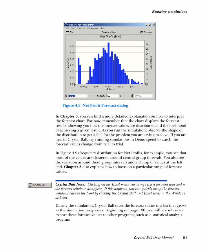
Running simulations1
Figure 4.9 Net Profit Forecast dialog
In Chapter 5, you can find a more detailed explanation on how to interpret the forecast chart. For now, remember that the chart displays the forecast results, showing you how the forecast values are distributed and the likelihood of achieving a given result. As you run the simulation, observe the shape of the distribution to get a feel for the problem you are trying to solve. If you are new to Crystal Ball, try running simulations in Demo speed to watch the forecast values change from trial to trial.
In Figure 4.9 (frequency distribution for Net Profit), for example, you see that most of the values are clustered around central group intervals. You also see the variation around these group intervals and a clump of values at the left end. Chapter 5 also explains how to focus on a particular range of forecast values.
Crystal Ball Note: Clicking on the Excel menu bar brings Excel forward and makes the forecast windows disappear. If this happens, you can quickly bring the forecast windows back to the front by clicking the Crystal Ball and Excel icons in the Windows task bar.
During the simulation, Crystal Ball saves the forecast values in a list that grows as the simulation progresses. Beginning on page 190, you will learn how to export these forecast values to other programs, such as a statistical analysis program.
Crystal Ball User Manual 91

Chapter 4 | Running Simulations
Running a simulationTo run a simulation:
1. Select Run > Start Simulation or click the Start Simulation button in the Crystal Ball toolbar.
If you set the forecast to appear in the Define Forecast dialog, a forecast window appears. As the simulation proceeds, the forecast chart updates to reflect the changing values in the forecast cell.
Crystal Ball Note: When you start Crystal Ball, the Crystal Ball Control Panel appears as shown in Figure 4.10 on page 94. You can use the Crystal Ball Control Panel to perform many of the procedures described in this section. For details, see “The Crystal Ball Control Panel” on page 93.
Stopping a simulationTo stop a simulation:
1. Select Run > Stop Simulation or click the Stop button on the Crystal Ball toolbar or Control Panel.
Continuing a simulationTo continue a simulation:
1. Select Run > Continue Simulation or click the Continue button on the Crystal Ball toolbar or Control Panel.
Resetting and rerunning a simulationTo reset the simulation and start over again:
1. Select Run > Reset Simulation or click the Reset button on the Crystal Ball toolbar or Control Panel.
A dialog appears with a message asking you to confirm your request to reset the simulation.
2. Click OK.
Crystal Ball resets the number of trials to 0 and clears the list of values and statistics for each assumption and forecast. However, the assumption and forecast definitions remain.
92 Crystal Ball User Manual

Running simulations1
3. Change any assumptions or forecasts as needed.
4. Select Run > Start Simulation or click the Run button on the Crystal Ball toolbar.
The simulation starts over again.
Single-steppingBefore you run a simulation or after you have stopped it, you can use the Single Step command to watch the simulation process generate one set of values (a trial) at a time for the assumption cells and recalculate the spreadsheet. This feature is useful if you are trying to track down a calculation error or verify that the values being produced for your assumption cells are valid.
To observe an individual trial:
1. Select Run > Reset Simulation or click the Reset button on the Crystal Ball toolbar or Control Panel.
2. Select Run > Single Step or click the Single-Step button to run one trial of the simulation. Click the button again to run another.
The Crystal Ball Control PanelYou can use the Crystal Ball Control Panel to perform many simulation and analysis commands. When you start the first run as described in “Running a simulation” on page 92, the Crystal Ball Control Panel appears as shown in Figure 4.10 on page 94.
Once it appears, you will find its buttons and menus convenient to use for stopping, continuing, resetting, single-stepping, and analyzing the results.
Run preference settings determine whether the Control Panel appears or is hidden when a simulation runs. To hide the Control Panel, uncheck Show Control Panel on the Options tab of the Run Preferences dialog (click the Run Preferences tool or choose Run > Run Preferences).
Crystal Ball Note: By default, the Control Panel stays open following a reset. To close it, uncheck Leave Open On Reset on the Options tab of the Run Preferences dialog. For more information on the Run Preferences Options tab, see “Options preferences” on page 86.
Crystal Ball User Manual 93

Chapter 4 | Running Simulations
Figure 4.10 The Crystal Ball Control Panel
When you click the More button, simulation statistics appear below the controls. They show how fast the simulation ran and how many assumptions, decision variables, and forecasts were included in it.
Figure 4.11 Control Panel with simulation statistics
Crystal Ball Note: Clicking on the Excel window title bar brings Excel forward and makes the forecast windows disappear. If this happens, you can quickly bring the forecast windows back to the front by clicking the Crystal Ball and Excel icons in the Windows task bar to display the chart windows again.
More button
Menubar
Progress bar
Task buttons
94 Crystal Ball User Manual

Managing chart windows1
The Crystal Ball Control Panel menubar
The following table describes the Control Panel menus and their commands:
Managing chart windowsYou can close the forecast and other chart windows at any time and the simulation will continue. Running a simulation with the windows closed decreases the time required to run the simulation.
Single windowsTo close one window, click the Close icon in the upper right corner of the chart window.
Table 4.6 Crystal Ball Control Panel menus
Menu Commands
Run Start Simulation/Continue Simulation (page 92) Reset Simulation (page 92) Single Step (page 93) Freeze (page 88) OptQuest Predictor Tools (page 198) Run Preferences (page 80)
Analyze Assumption Charts (page 18) Forecast Charts (page 59) Overlay Charts (page 146) Trend Charts (page 154) Sensitivity Charts (page 165) Cascade (Table 4.7 on page 96) Close All (Table 4.7 on page 96) Create Report (page 182) Extract Data (page 190) Save Results (page 97) Restore Results (page 98)
Help Control Panel Help
Crystal Ball User Manual 95

Chapter 4 | Running Simulations
Multiple windowsYou can use several commands on the Analyze menu and Crystal Ball toolbar to:
• Close and cascade all open forecast windows and other chart windows.
• Open charts that have been closed.
• Create new charts.
• Delete overlay, trend, and sensitivity charts.
These commands are listed in Table 4.7, following.
Also see “Speed preferences” on page 84 for ways to control whether and how often chart windows display and redraw.
To manage multiple windows:
• Click a chart button in the Crystal Ball toolbar to open all windows for that chart type, or
• Choose from the commands listed in Table 4.7.
Table 4.7 Crystal Ball window management commands
Button Command Effect
Analyze > Open Selected Cells Opens charts for all assumption and forecast cells in the selected range.
Analyze > Assumption Charts Opens a dialog so you can choose which assumption charts to open or close.
Analyze > Forecast Charts Opens a dialog so you can choose which forecast charts to open or close.
Analyze > Overlay Charts Opens a dialog so you can choose which overlay charts to open or close, create, or delete.
Analyze > Trend Charts Opens a dialog so you can choose which trend charts to open or close, create, or delete.
Analyze > Sensitivity Charts Opens a dialog so you can choose which sensitivity charts to open or close, create, or delete.
96 Crystal Ball User Manual
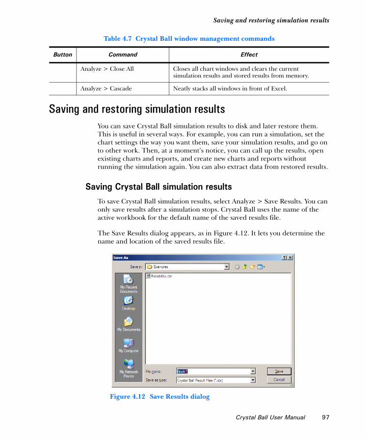
Saving and restoring simulation results1
Saving and restoring simulation resultsYou can save Crystal Ball simulation results to disk and later restore them. This is useful in several ways. For example, you can run a simulation, set the chart settings the way you want them, save your simulation results, and go on to other work. Then, at a moment’s notice, you can call up the results, open existing charts and reports, and create new charts and reports without running the simulation again. You can also extract data from restored results.
Saving Crystal Ball simulation resultsTo save Crystal Ball simulation results, select Analyze > Save Results. You can only save results after a simulation stops. Crystal Ball uses the name of the active workbook for the default name of the saved results file.
The Save Results dialog appears, as in Figure 4.12. It lets you determine the name and location of the saved results file.
Figure 4.12 Save Results dialog
Analyze > Close All Closes all chart windows and clears the current simulation results and stored results from memory.
Analyze > Cascade Neatly stacks all windows in front of Excel.
Table 4.7 Crystal Ball window management commands
Button Command Effect
Crystal Ball User Manual 97

Chapter 4 | Running Simulations
Crystal Ball saves the simulation results, including charts and reports, in a file with extension .cbr. Once you have saved the simulation results you can continue working with Crystal Ball.
Crystal Ball Note: If you choose Analyze > Save Results, only results from the current simulation are saved. Previously restored results are not saved. This can be an issue where both current and saved results are used, for example, in overlay charts. Suppose current and restored forecasts are both used in an overlay chart. If the overlay chart is then saved as part of the current simulation results, when it is restored it will only contain forecasts from the saved current results set. Forecasts from the previously restored results will no longer be included in the chart.
Restoring Crystal Ball simulation resultsTo restore Crystal Ball simulation results that you saved earlier, select Analyze > Restore Results. The Restore Results dialog appears, as shown in Figure 4.13.
Figure 4.13 Restore Results dialog
The file list contains only files that have the .cbr file type. Select the results file you want to restore and click Open. If you try to open a file that is not Crystal Ball saved results, or if Crystal Ball recognizes that a saved results file has somehow been damaged, you will not be able to open the file, and an error message appears.
98 Crystal Ball User Manual
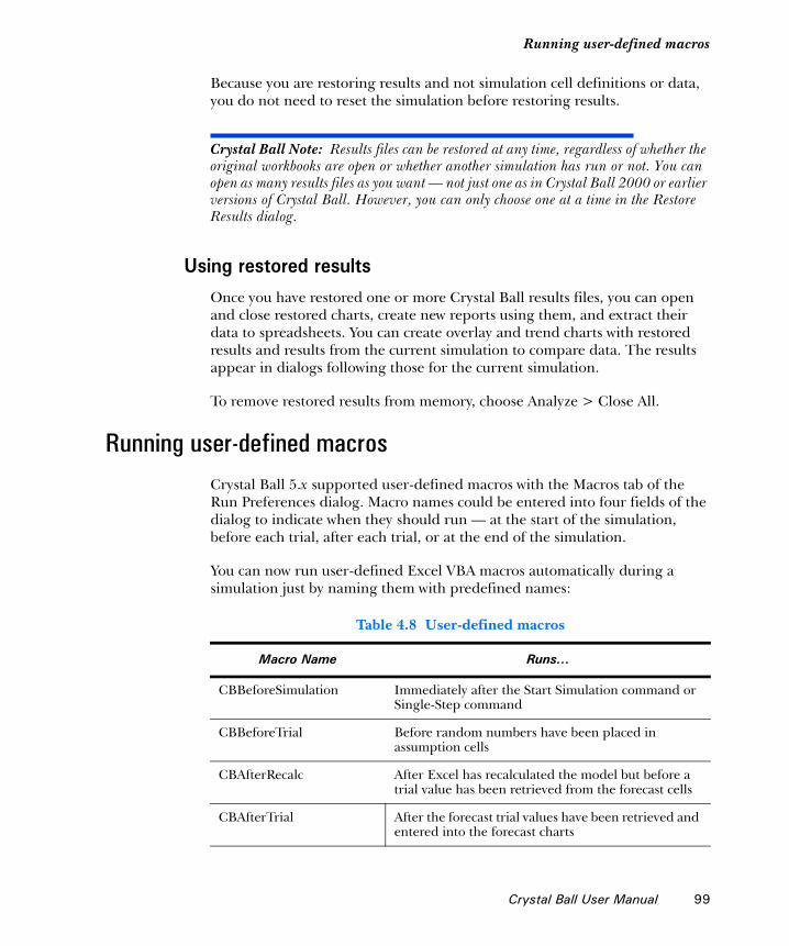
Running user-defined macros1
Because you are restoring results and not simulation cell definitions or data, you do not need to reset the simulation before restoring results.
Crystal Ball Note: Results files can be restored at any time, regardless of whether the original workbooks are open or whether another simulation has run or not. You can open as many results files as you want — not just one as in Crystal Ball 2000 or earlier versions of Crystal Ball. However, you can only choose one at a time in the Restore Results dialog.
Using restored resultsOnce you have restored one or more Crystal Ball results files, you can open and close restored charts, create new reports using them, and extract their data to spreadsheets. You can create overlay and trend charts with restored results and results from the current simulation to compare data. The results appear in dialogs following those for the current simulation.
To remove restored results from memory, choose Analyze > Close All.
Running user-defined macrosCrystal Ball 5.x supported user-defined macros with the Macros tab of the Run Preferences dialog. Macro names could be entered into four fields of the dialog to indicate when they should run — at the start of the simulation, before each trial, after each trial, or at the end of the simulation.
You can now run user-defined Excel VBA macros automatically during a simulation just by naming them with predefined names:
Table 4.8 User-defined macros
Macro Name Runs...
CBBeforeSimulation Immediately after the Start Simulation command or Single-Step command
CBBeforeTrial Before random numbers have been placed in assumption cells
CBAfterRecalc After Excel has recalculated the model but before a trial value has been retrieved from the forecast cells
CBAfterTrial After the forecast trial values have been retrieved and entered into the forecast charts
Crystal Ball User Manual 99
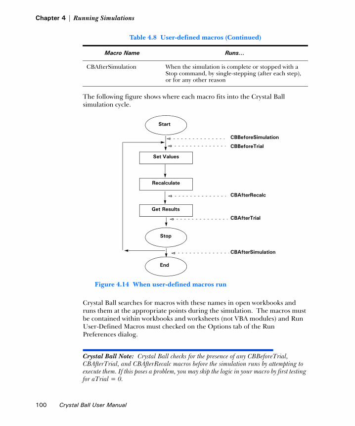
Chapter 4 | Running Simulations
The following figure shows where each macro fits into the Crystal Ball simulation cycle.
Figure 4.14 When user-defined macros run
Crystal Ball searches for macros with these names in open workbooks and runs them at the appropriate points during the simulation. The macros must be contained within workbooks and worksheets (not VBA modules) and Run User-Defined Macros must checked on the Options tab of the Run Preferences dialog.
Crystal Ball Note: Crystal Ball checks for the presence of any CBBeforeTrial, CBAfterTrial, and CBAfterRecalc macros before the simulation runs by attempting to execute them. If this poses a problem, you may skip the logic in your macro by first testing for aTrial = 0.
CBAfterSimulation When the simulation is complete or stopped with a Stop command, by single-stepping (after each step), or for any other reason
Table 4.8 User-defined macros (Continued)
Macro Name Runs...
Start
Set Values
Recalculate
Get Results
Stop
CBBeforeSimulation
CBBeforeTrial
CBAfterRecalc
CBAfterTrial
End
CBAfterSimulation
100 Crystal Ball User Manual
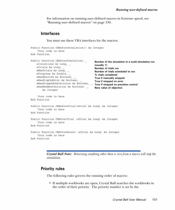
Running user-defined macros1
For information on running user-defined macros in Extreme speed, see “Running user-defined macros” on page 330.
InterfacesYou must use these VBA interfaces for the macros:
Crystal Ball Note: Returning anything other than a zero from a macro will stop the simulation.
Priority rulesThe following rules govern the running order of macros:
• If multiple workbooks are open, Crystal Ball searches the workbooks in the order of their priority. The priority number is set by the
Public Function CBBeforeSimulation() As Integer'Your code is here
End Function
Public Function CBAfterSimulation( _aIterations As Long, _aTrials As Long, _aMaxTrials As Long, _aProgress As Double, _aWasAborted As Boolean, _aWasStopOnError As Boolean, _aWasStoppedOnPrecision As Boolean, _aHasNewBestSolution As Boolean) _
As Integer
'Your code is hereEnd Function
Public Function CBBeforeTrial(aTrial As Long) As Integer'Your code is here
End Function
Public Function CBAfterTrial (aTrial As Long) As Integer'Your code is here
End Function
Public Function CBAfterRecalc (aTrial As Long) As Integer'Your code is here
End Function
Number of the simulation in a multi-simulation run (usually 1) Number of trials run Number of trials scheduled to run % trials completed True if manually stopped True if stopped on error True if stopped on precision controlNew value of objective
Crystal Ball User Manual 101

Chapter 4 | Running Simulations
CB.SetCBWorkbookPriority macro. If this macro has not been called on the workbook, no workbook order is guaranteed.
Crystal Ball Note: CB.SetCBWorkbookPriority sets the running order for macros when multiple workbooks are open. For example, a workbook with order=10 will run before a workbook with order=20. CB.SetCBWorkbookPriority runs only at the workbook level and not at the worksheet level.
The definition of this macro is:
Public Function CB.SetCBWorkbookPriority (aPriority As Long)
A syntax example, used in a subroutine at the module level, is:
Application.Workbooks("Book1.xls").Activate CB.SetCBWorkbookPriority(10)
This example assigns a priority of 10 to the workbook Book1.xls.
• Within each workbook, macros on worksheets run in left-to-right sheet order in the workbook provided there are no macros at the workbook level. If there are macros at the workbook level, macros in that workbook at the worksheet level do not run.
• If there are no Crystal Ball data cells in a workbook, no macros run against it.
• Macros in modules are not supported.
Global macrosIf you want to run certain macros with any or all of your Crystal Ball models, you need to make sure that the workbook containing those macros is open in Excel. Then, you can use calls within each model to run those macros as required.
Previous versions of Crystal Ball handled global macros differently. Now, you can run specific macros only for certain models and are no longer required to turn the macros on and off depending on the model that is being run.
Toolbar macrosIf you want to use custom Excel toolbar macros defined in a separate workbook while Crystal Ball is loaded, be sure to save that workbook to the folder C:\Documents and Settings\yourname\Application Data\Microsoft\Excel\XLSTART.
102 Crystal Ball User Manual
Chapter 5Analyzing Forecast Charts
In this chapter• Guidelines for analyzing simulation results
• Understanding and using forecast charts
• Setting chart preferences
• Managing existing charts
This chapter describes how to use forecast charts to analyze simulation results. As you read through the chapter, you will learn to focus on a particular range of simulation results, analyze forecast charts, and interpret relevant descriptive statistics.
You will also learn how to customize forecast charts, work with chart windows, and share charts with other applications.
The next chapter introduces additional charts. Chapter 7 describes how to extract Crystal Ball simulation data for use in Excel and other applications and how to prepare reports.
Crystal Ball User Manual 103

Chapter 5 | Analyzing Forecast Charts
Guidelines for analyzing simulation resultsWhile a simulation runs, Crystal Ball creates a forecast chart for each forecast cell. Forecast charts condense much information into a small space. You can display that information in several different ways, both graphically and numerically.
When you analyze a simulation, you can focus on forecast charts. You can also display other kinds of charts, generate reports, and extract data for further processing using Excel or other analysis tools.
The following steps can help guide your simulation analysis by focusing on details as well as general trends:
1. Look at the “big picture.”
Consider each forecast chart from a high-level viewpoint. Look at the shape of the distribution:
• Is it distributed normally or skewed negatively or positively?
• Is it “flat” (spread out on both sides of the mean) or “peaked” (with most values clustered closely around the mean)?
• Does it have a single mode (most likely value) or is it bimodal with several “peaks” or “humps”?
• Is it continuous or are there groups of values separated from the rest, maybe even extreme “outliers” that fall outside of the display range?
The statistical concepts in the “Statistical Definitions” chapter of the online Crystal Ball Reference Manual can help with this part of your analysis.
2. Look at the certainty level, the probability of achieving values within a certain range.
You can enter a range, such as all values greater than $0 dollars if you’re analyzing profits, and view the certainty of falling within the range ($0 to + Infinity, in this case). You can also enter a certainty, say 75%, and see what range of values would be required to meet that level. “Determining the certainty level” beginning on page 107 explains these and other ways of analyzing certainty.
3. Focus on the display range.
You can change the display range to focus on different sections of the forecast chart. For example, you can set the display range to focus on just the upper or lower tail of the forecast. “Focusing on the display range” on page 112 discusses this analysis technique.
104 Crystal Ball User Manual

Guidelines for analyzing simulation results1
4. Look at different views of the forecast.
Use the View menu to switch among different ways of viewing the forecast distribution graphically (frequency, cumulative frequency, or reverse cumulative frequency) or numerically (statistics, percentiles, goodness of fit data, or capability metrics). You can also choose whether to show charts and statistics simultaneously or separately. For instructions, see “Changing the distribution view and interpreting statistics” on page 115.
5. Customize the forecast chart.
Use the chart preferences to change graphic presentations from bars to areas or lines, or experiment with different colors, 2D versus 3D, more or fewer plotted intervals or data points, and other display variations. “Setting chart preferences” beginning on page 128 describes the many ways you can format charts for analysis and presentation of results.
6. Create other kinds of charts.
You can display overlay charts (page 146), trend charts (page 154), and sensitivity charts (page 165). As with forecast charts, you can customize these charts as well. Selecting different views of the data can help you analyze it and present it to others.
7. Create reports.
Create reports with charts and data (page 182). You can quickly produce pre-defined or custom reports for analysis and presentation.
8. Extract data for numeric analysis and presentation.
You can extract simulation results to Excel for further analysis or for further export into other analytical tools. See “Extracting data” on page 190 for details.
9. Use other Crystal Ball tools for different types of analyses.
Depending on the types of problems you are analyzing, the Crystal Ball Batch Fit, Bootstrap, Correlation Matrix, Decision Table, Scenario Analysis, Tornado Chart, and 2D Simulation tools offer addition analysis techniques. These tools are described in Chapter 8. If you have Crystal Ball Professional or Premium Edition, you can also use OptQuest and CB Predictor for optimization and time-series analysis.
Crystal Ball User Manual 105

Chapter 5 | Analyzing Forecast Charts
Understanding and using forecast chartsAs discussed in the section “About Crystal Ball simulations” on page 78, forecast charts use frequency distributions to show the number (frequency) of values occurring in a given interval. The highest value on the frequency scale to the right of the chart is the frequency for the interval that contains the greatest number of forecast values — the mode of the graphed distribution. You can estimate the frequency for other points on the forecast chart using this frequency scale.
Crystal Ball Note: You can now display forecast charts in Split View, which shows charts and statistics side by side. This section focuses on each type of chart separately. For more information about Split View and its features, see “Using Split View” on page 122.
The highest value on the probability scale to the left of the chart is the probability for the mode. You can estimate the probability for other points on the forecast chart using this probability scale.
In the example below, the mode (in the middle of the distribution) has a frequency of 32, meaning that there are 32 values in the interval expressed by that column. The mode has a probability of 0.065 (or 6.5%), meaning that there is a 6.5% chance of a value falling within this interval.
Figure 5.1 shows the elements of the forecast chart.
Figure 5.1 Forecast chart
Number of trials
Certainty level
Number of trials displayed
Certainty range
Certainty grabbers
106 Crystal Ball User Manual

Understanding and using forecast charts1
Crystal Ball forecasts the entire range of results for a given situation. However, the forecast chart shows only the display range, which is a subrange of the whole. By default, the display range includes all trials within 2.6 standard deviations of the mean (approximately 99% of the forecast values). Crystal Ball then rounds the display range to the next even number of units. For this reason, outlying trials might be excluded from the display range.
Crystal Ball Note: To display all trials, change the chart axis preferences to display fixed endpoints between –Infinity and +Infinity (for instructions, see “Focusing on the display range” on page 112).
The number of trials run for this forecast appears in the upper left corner of the forecast chart. The number of trials shown (the number of trials run minus the number of outlying values) appears in the upper right corner. The display range is the linear distance from about ($15.00) to $35.00, as shown in Figure 5.1.
Determining the certainty levelThe forecast chart also shows the certainty range for the forecast. In Crystal Ball, the certainty range includes all trials between the certainty grabbers. In the next section, you will learn how to change the certainty range.
Crystal Ball Note: When the certainty grabbers are at –Infinity and +Infinity, the certainty range includes every forecast value regardless of the size of the display range.
Crystal Ball compares the number of values in the certainty range with the number of values in the entire range to calculate the certainty level for the forecast. The example in Figure 5.1 shows a certainty level of 100% since the default certainty range includes all possible values. By default, Crystal Ball calculates the certainty level based on the entire range of forecast values.
On either side of the Certainty field, the certainty minimum and maximum appear.
The certainty level is one of Crystal Ball’s key statistics because it shows the probability of achieving the values within a specific range. With Crystal Ball, you can determine the certainty level for specific value ranges either by moving the certainty grabbers on the forecast chart or typing the certainty minimum and maximum in the fields. You can also type a certainty level in the certainty field to get a certainty range centered around the median.
Crystal Ball User Manual 107

Chapter 5 | Analyzing Forecast Charts
When you move the certainty grabbers, the certainty range changes and Crystal Ball recalculates the certainty level. When you type minimum and maximum values, Crystal Ball moves the certainty grabbers for you and recalculates the certainty level. When you type the certainty level in the certainty field, Crystal Ball moves the certainty grabbers to show you the value range for the certainty level you specified.
Moving certainty grabbers
To determine the certainty level for a specific value range using certainty grabbers:
1. Make sure the forecast chart you want to use is the active (selected) window.
2. Move the certainty grabbers on the forecast chart, as shown in Figure 5.2.
Figure 5.2 Moving the left certainty grabber
The certainty minimum field shows the value that corresponds to the position of the left certainty grabber; the certainty maximum field shows the value that corresponds to the position of the right certainty grabber. The Certainty field shows the certainty level for the area between the certainty grabbers. Crystal Ball shades the columns outside the certainty grabbers a different color to show that those values have been excluded, as illustrated in Figure 5.3.
Click the certainty grabber and drag it when the cursor changes to a hand.
108 Crystal Ball User Manual
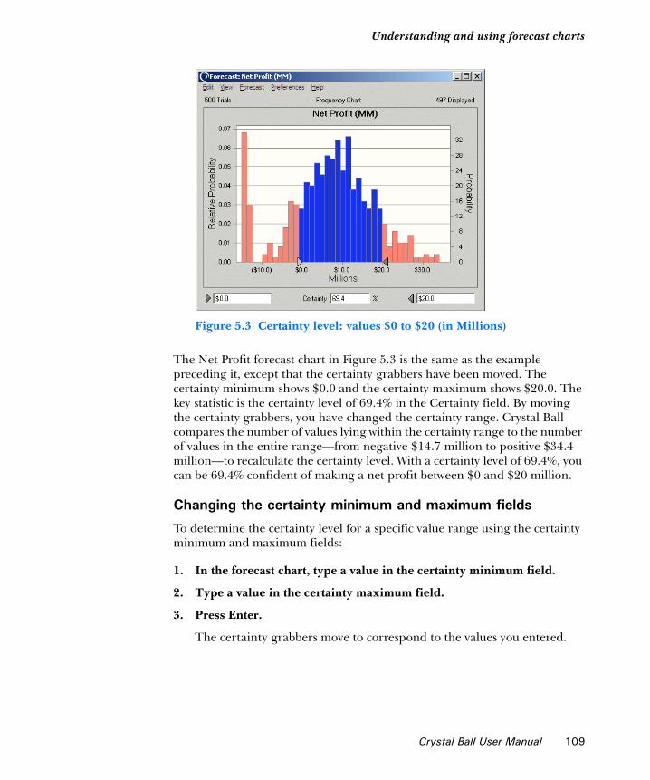
Understanding and using forecast charts1
Figure 5.3 Certainty level: values $0 to $20 (in Millions)
The Net Profit forecast chart in Figure 5.3 is the same as the example preceding it, except that the certainty grabbers have been moved. The certainty minimum shows $0.0 and the certainty maximum shows $20.0. The key statistic is the certainty level of 69.4% in the Certainty field. By moving the certainty grabbers, you have changed the certainty range. Crystal Ball compares the number of values lying within the certainty range to the number of values in the entire range—from negative $14.7 million to positive $34.4 million—to recalculate the certainty level. With a certainty level of 69.4%, you can be 69.4% confident of making a net profit between $0 and $20 million.
Changing the certainty minimum and maximum fields
To determine the certainty level for a specific value range using the certainty minimum and maximum fields:
1. In the forecast chart, type a value in the certainty minimum field.
2. Type a value in the certainty maximum field.
3. Press Enter.
The certainty grabbers move to correspond to the values you entered.
Crystal Ball User Manual 109

Chapter 5 | Analyzing Forecast Charts
Entering certainty directly
Alternately, you can type the certainty level on the forecast chart and let Crystal Ball calculate the minimum and maximum for you. Make sure that the certainty grabbers are free (whenever you click an certainty grabber, it turns to a lighter color and is considered anchored). To free the lighter color certainty grabber, click it. Then when you type in a certainty level, you will center the certainty range on the median statistic.
Crystal Ball Note: To free or anchor both certainty grabbers, press Ctrl-click or Shift-click.
In the following procedure you will enter a certainty level of 10% and watch Crystal Ball move the certainty grabbers:
1. Press Ctrl-click (or Shift-click) until both certainty grabbers are free (a lighter color).
2. Type 10 in the Certainty field.
3. Press Enter.
Crystal Ball moves the certainty grabbers to include 10% of the trials centered around the median statistic of the entire range.
Anchoring a grabber, then entering certainty
You can also anchor a certainty grabber, type the certainty level, and Crystal Ball moves the free grabber to correspond to the value range for the level.
1. Move the left certainty grabber until the certainty minimum value is $0.0.
The certainty grabber turns to a lighter color and is considered anchored.
2. Type 75 in the Certainty field.
3. Press Enter.
Crystal Ball moves the free certainty grabber toward the anchored certainty grabber to include 75% of the values as in Figure 5.4.
Crystal Ball Note: If both grabbers are free, the distribution is centered on the median.
110 Crystal Ball User Manual

Understanding and using forecast charts1
Figure 5.4 Certainty level: 75% from left certainty grabber
You also can cross over the certainty grabbers to determine the certainty level for the two tails (ends).
You can determine the certainty level for specific value ranges at any time, either during or after the simulation.
Resetting the certainty range
To reset the original certainty range before beginning the next section:
1. In the forecast chart, either:
• Move the right certainty grabber until the certainty maximum field shows positive infinity, or
• Type +Infinity in the right field
2. Either:
• Move the left certainty grabber until the certainty minimum field shows negative infinity, or
• Type –Infinity in the left field
The forecast chart displays a certainty level of 100%, as displayed in the original forecast.
Crystal Ball User Manual 111

Chapter 5 | Analyzing Forecast Charts
Focusing on the display rangeWith Crystal Ball, you can focus on a particular range of the forecast results by changing axis settings in the Chart Preferences dialog. For instructions, see “Customizing chart axes and axis labels” on page 138.
Using the Scale group of axis settings, you can define the display range in the following ways.
By default, the x-axis value numbers are automatically adjusted to round numbers to make the forecasts easier to read. The Axis chart preference settings include Round Display Range, which constrains the display range to round numbers. You can uncheck this setting to display actual, unrounded numbers.
Other chart customizations are available to help you interpret the results of the simulation by viewing the data in different ways. For details, see “Setting chart preferences” beginning on page 128.
Crystal Ball Note: Also see “Setting preferences with hot keys” on page 129 for ways to change the appearance of charts without using menu commands.
Table 5.1 Chart Preferences > Axis > Scale > Type settings
Type Setting Effect
Auto Crystal Ball uses a default display range of 2.6 standard deviations from the mean, which includes about 99% of the forecast values. (See Standard Deviation, following.)
Fixed Sets the display range end points manually.Using fixed end points for the display range lets you focus on particular value ranges. For example, you can focus on positive values only to look at the profit for a profit/loss forecast.
Standard Deviation Sets the display range end points in terms of standard deviations; defines the number of standard deviations worth of value you want to display on each side of the mean and centers values around the mean.If you choose to set the display range in terms of standard deviations, you could change the display range to 1 standard deviation from the mean to look at approximately 68% of the forecast values.
Percentile Sets the display range end points in terms of percentiles.
112 Crystal Ball User Manual
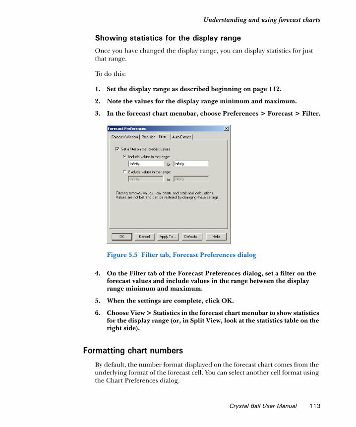
Understanding and using forecast charts1
Showing statistics for the display range
Once you have changed the display range, you can display statistics for just that range.
To do this:
1. Set the display range as described beginning on page 112.
2. Note the values for the display range minimum and maximum.
3. In the forecast chart menubar, choose Preferences > Forecast > Filter.
Figure 5.5 Filter tab, Forecast Preferences dialog
4. On the Filter tab of the Forecast Preferences dialog, set a filter on the forecast values and include values in the range between the display range minimum and maximum.
5. When the settings are complete, click OK.
6. Choose View > Statistics in the forecast chart menubar to show statistics for the display range (or, in Split View, look at the statistics table on the right side).
Formatting chart numbersBy default, the number format displayed on the forecast chart comes from the underlying format of the forecast cell. You can select another cell format using the Chart Preferences dialog.
Crystal Ball User Manual 113

Chapter 5 | Analyzing Forecast Charts
To change the format of numbers in a forecast chart:
1. In the forecast window, choose Preferences > Chart.
The Chart Preferences dialog appears.
2. Click the Axis tab.
Find the Format Number group as shown in Figure 5.6.
Figure 5.6 The Format Number group on the Axis tab
3. Choose a format from the drop-down list, shown in Figure 5.7. They are similar to Excel formats.
Figure 5.7 Format settings
For most formats, you can also specify the number of decimal places and whether to use a thousands separator.
4. Click OK to apply the settings, or use Apply To as described on page 139.
114 Crystal Ball User Manual

Understanding and using forecast charts1
Changing the distribution view and interpreting statisticsThe forecast settings related to distribution type determine the overall appearance of a forecast chart. You can also choose to display a table of statistics or percentiles instead of or in addition to a chart.
To set the distribution type or display a data table:
1. Open the View menu in the forecast window.
2. Choose a distribution type or other view to display on the forecast chart as described in Table 5.2.
The following sections show examples of each View type.
Table 5.2 Forecast Preferences dialog, Forecast Window > View settings
View Setting Effect
Frequency Shows the number or frequency of values occurring in a given interval. This is the default distribution type.
Cumulative Frequency Shows the number or proportion (percentage) of values less than or equal to a given amount.
Reverse Cumulative Frequency
Shows the number or proportion (percentage) of values greater than or equal to a given amount.
Statistics Shows a full set of descriptive statistics for a simulation in the forecast window.
Percentiles Shows percentile information in 10% increments, where a percentile is the percent chance, or probability, of a forecast value being less than or equal to the value that corresponds to the percentile (by default).
Goodness Of Fit If distribution fitting is selected in the Forecast or Preferences > Forecast menus, shows goodness-of-fit statistics for the selected distribution and ranking method.
Capability Metrics If process capability metrics are set for display, shows a table of process capability (quality) statistics for the simulation. See “Viewing capability metrics” on page 344 for more information.
Split View When selected, shows all selected views simultaneously. For details, see “Using Split View” on page 122.
Crystal Ball User Manual 115

Chapter 5 | Analyzing Forecast Charts
FrequencyFrequency, the default forecast view, shows a simple count of values (the frequency) for each interval on the x-axis. Figure 5.8 shows a frequency chart of net profit values for a simulation where there is a 75% probability of net profit falling between $0.00 and $26.1 million. The chart has a median of $7.8 million. This is also the 50th percentile. By default, there is a 50% probability that net profit will be at or below this value.
Figure 5.8 Forecast chart — frequency
Cumulative frequencyFigure 5.9 shows the Net Profit forecast chart as a cumulative distribution. This chart shows the number or proportion (percentage) of values less than or equal to a given amount.
Figure 5.9 Forecast chart—cumulative frequency
116 Crystal Ball User Manual

Understanding and using forecast charts1
To create this chart, the frequencies are added cumulatively, starting from the lower end of the range, and then plotted as a cumulative frequency curve. To understand the cumulative distribution, look at a particular value, $7.8 million (in the example above). The chart shows that the probability of $7.8 million is about 50%; approximately 50% of the values are less than $7.8 million, while approximately 50% are greater. This would be correct for a median value. Note also that the chart shows that the probability for $26.1 million is about .95 while the probability for $0 is about .20. This is also correct, since the probability of Net Profit falling between those two values is .75 (.95 – .20 = .75) or Certainty = 75%.
Reverse cumulative frequencyFigure 5.10 shows the Net Profit forecast chart as a reverse cumulative distribution. This chart shows the number or proportion (percentage) of values greater than or equal to a given amount.
Figure 5.10 Forecast chart—reverse cumulative frequency
To create this chart, the frequencies are added cumulatively starting at the higher end of the range, and then plotted as a declining cumulative frequency curve. To understand the reverse cumulative distribution, look at a particular value, $7.8 million (in the example above). The chart shows that the probability of $7.8 million is about 50%; approximately 50% of the values are less than $7.8 million, while approximately 50% are greater. This would be correct for a median value. Note also that the chart shows that the probability for $26.1 million is about .05 (of having a greater value) while the probability for $0 is about .80. This is also correct, since the probability of Net Profit falling between those two values is .75 (.80 – .05 = .75) or Certainty = 75%. Notice in this chart that the reverse cumulative frequency values are
Crystal Ball User Manual 117

Chapter 5 | Analyzing Forecast Charts
complements of the cumulative frequency values: .20 + .80 = 1.00 and .95 + .05 = 1.0 (the probability values for $0.0 and $26.1 million, respectively).
StatisticsYou can display a full set of descriptive statistics for a simulation in the forecast window by choosing View > Statistics.
Figure 5.11 Forecast window—statistics
The example in Figure 5.11 shows statistics for the entire range of values (100% of the forecast values, including the outliers — extreme values excluded from the default display range). Statistical terms listed on this table are discussed in the “Statistical Definitions” chapter of the online Crystal Ball Reference Manual and the glossary.
Crystal Ball Note: If the Precision Control feature is checked in the Run Preferences dialog and the forecast has Precision Control options set, the Precision column appears in the Statistics view.
PercentilesYou can display percentile information in 10% increments in the forecast window by choosing View > Percentiles. A percentile is the percent chance, or probability, of a forecast value being less than or equal to the value that corresponds to the percentile (the default). For example, Figure 5.12 displays the percentile view of the Net Profit forecast, where the 90th percentile corresponds to $19.3 million, meaning that there is a 90% chance of a forecast value being equal to or less than $19.3 million. Another interpretation is that 90% of the forecast values are equal to or less than $19.3 million.
Notice that the Median in Statistics view is the same as the 50th percentile in Percentiles view — in this case, $7.8 million.
118 Crystal Ball User Manual

Understanding and using forecast charts1
Figure 5.12 Forecast—Percentiles view
Crystal Ball Note: If the Precision Control feature is checked in the Run Preferences dialog and the forecast has Precision Control options set, the Precision column appears in the Percentiles view.
Goodness Of FitIf you have selected distribution fitting, described in the next section, you can choose the Goodness Of Fit view to display comparative fit statistics for each of the selected distribution types. The distributions are ordered according to the selected ranking method. Figure 5.13 shows statistics for each ranking method and each continuous distribution type. Notice that Beta is ranked highest for all three methods for this forecast.
Figure 5.13 Forecast—Goodness Of Fit view
Crystal Ball User Manual 119

Chapter 5 | Analyzing Forecast Charts
Capability MetricsIf the process capability features are activated on the Statistics tab of the Run Preferences dialog and if either an LSL, USL, or both are entered into the Define Forecast dialog, the Capability Metrics view is available for the forecast chart. For a definition of each statistic, see “Capability metrics list” on page 353.
Figure 5.14 Capability Metrics view
Split ViewSplit View, shows forecast charts and related statistics onscreen at the same time. For more information, see “Using Split View” on page 122.
Fitting a distribution to a forecast
You can fit distributions to forecast charts, a feature that is similar to distribution fitting for assumptions (described beginning on page 27).
You can fit distributions to forecasts two ways:
• You can choose Forecast > Fit Probability Distributions in the forecast chart menubar to do a quick fit with the default or currently selected distributions and ranking method. You can also use this command to switch off distribution fitting that is set with either the Forecast menu or Preferences menu.
• You can choose Preferences > Forecast > Forecast Window in the forecast chart menubar to specify particular distributions and to choose one of
120 Crystal Ball User Manual
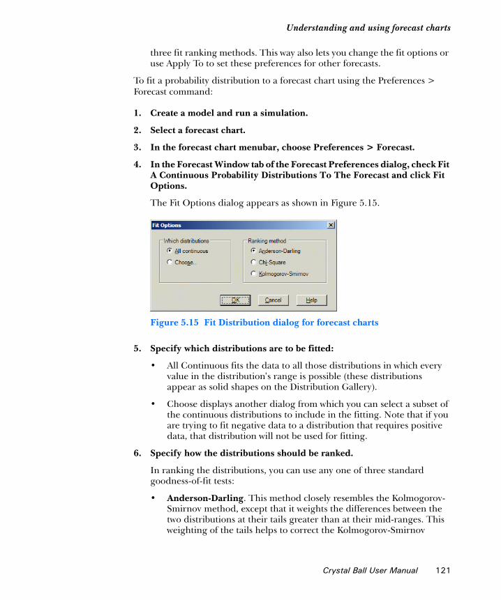
Understanding and using forecast charts1
three fit ranking methods. This way also lets you change the fit options or use Apply To to set these preferences for other forecasts.
To fit a probability distribution to a forecast chart using the Preferences > Forecast command:
1. Create a model and run a simulation.
2. Select a forecast chart.
3. In the forecast chart menubar, choose Preferences > Forecast.
4. In the Forecast Window tab of the Forecast Preferences dialog, check Fit A Continuous Probability Distributions To The Forecast and click Fit Options.
The Fit Options dialog appears as shown in Figure 5.15.
Figure 5.15 Fit Distribution dialog for forecast charts
5. Specify which distributions are to be fitted:
• All Continuous fits the data to all those distributions in which every value in the distribution’s range is possible (these distributions appear as solid shapes on the Distribution Gallery).
• Choose displays another dialog from which you can select a subset of the continuous distributions to include in the fitting. Note that if you are trying to fit negative data to a distribution that requires positive data, that distribution will not be used for fitting.
6. Specify how the distributions should be ranked.
In ranking the distributions, you can use any one of three standard goodness-of-fit tests:
• Anderson-Darling. This method closely resembles the Kolmogorov-Smirnov method, except that it weights the differences between the two distributions at their tails greater than at their mid-ranges. This weighting of the tails helps to correct the Kolmogorov-Smirnov
Crystal Ball User Manual 121

Chapter 5 | Analyzing Forecast Charts
method’s tendency to over-emphasize discrepancies in the central region.
• Chi-Square. This test is the oldest and most common of the goodness-of-fit tests. It gauges the general accuracy of the fit. The test breaks down the distribution into areas of equal probability and compares the data points within each area to the number of expected data points.
• Kolmogorov-Smirnov. The result of this test is essentially the largest vertical distance between the two cumulative distributions.
7. Click OK to perform the fit.
Crystal Ball Note: During a simulation, Crystal Ball disables distribution fitting on forecast charts and overlay charts after 1,000 trials and until the simulation stops to enhance performance. A final fit is performed at end of the simulation.
Using Split ViewSplit View displays charts and statistics at the same time. If you are using Crystal Ball’s process capability features, Split View is the default. Otherwise, you can activate Split View through the View menu or the Preferences > Forecast menu in the forecast chart window.
To activate Split View:
1. In the forecast window, choose View to open the View menu.
2. Choose Split View at the bottom of the menu.
The Frequency chart and statistics both appear, similar to the next figure.
122 Crystal Ball User Manual

Understanding and using forecast charts1
Figure 5.16 Frequency chart and statistics in Split view
You can resize the window and use the vertical pane splitter to adjust the size of the chart and the statistics pane.
3. If you want, continue opening the View menu and choosing charts or data.
The following figure shows a Frequency chart, a Cumulative Frequency chart, plus Statistics and Percentiles tables.
vertical pane splitter
Crystal Ball User Manual 123

Chapter 5 | Analyzing Forecast Charts
Figure 5.17 Frequency and Cumulative Frequency charts with statistics and percentiles in Split View
You can click in any of the Split View panes and use the chart hot keys to modify them without using the View or Preferences menus. For a list, see Table 5.5 on page 129.
You can also resize the chart window and drag the horizontal and vertical pane splitters to resize each part of the Split View window.
To clear Split View or remove any of the views from the window, open the View menu and uncheck each view you want to close.
horizontal pane splitter
124 Crystal Ball User Manual

Understanding and using forecast charts1
Setting forecast preferencesYou can set a number of specific forecast preferences to customize how Crystal Ball calculates and displays your forecast charts. These are in addition to the general chart preferences discussed starting on page 128.
Table 5.3 summarizes forecast features you can control with preference settings and refers to the table or section that describes each setting.
Basic instructions for setting forecast preferences
Like the chart preferences, forecast preferences can be set differently for each forecast chart.
To set forecast preferences:
1. Choose Preferences > Forecast in a forecast chart’s menubar.
The Forecast Preferences dialog appears, as shown in Figure 5.18.
Table 5.3 Available forecast preference settings
How Do I ...? Described in...
Change the forecast chart view Table 3.1 on page 63
Determine when the forecast window appears Table 3.1 on page 63
Fit a distribution to the forecast Table 3.1 on page 63
Set precision controls for forecast statistics Table 3.2 on page 65
Filter ranges of forecast values Table 3.3 on page 67
Automatically extract forecast data to a spreadsheet
Table 3.4 on page 69
Crystal Ball User Manual 125

Chapter 5 | Analyzing Forecast Charts
Figure 5.18 The Forecast Preferences dialog
2. Click a tab and set preferences as required.
These tabs also appear in the expanded Define Forecast dialog. For details see the following sections or click the Help button in the Forecast Preferences dialog:
• “Forecast Window preferences” on page 62 — manage window display and distribution fitting for the forecast.
• “Precision preferences” on page 64 — manage precision control settings.
• “Filter preferences” on page 66 — let you discard values inside or outside a range for the current forecast.
• “Auto Extract preferences” on page 68 — let you specify which statistics to extract automatically to Excel when a simulation stops.
Also see the previous section, “Setting forecast preferences” on page 125.
Crystal Ball Note: For more information on setting the Precision Control option and settings, see “Precision control” on page 318. See “Confidence intervals” in the “Statistical Definitions” chapter of the online Crystal Ball Reference Manual for more information about how absolute and relative precision relate to the confidence interval.
3. If you want to reset forecast preference defaults to the original settings shipped with Crystal Ball, click Defaults.
4. To copy preferences to other forecasts, click Apply To.
126 Crystal Ball User Manual

Understanding and using forecast charts1
You can specify whether to apply all forecast preferences or just the current tab and whether to apply them to the current Excel sheet, all sheets in the workbook, or all open and new workbooks.
5. When all settings are complete, click OK to apply them.
Setting forecast chart preferencesThe chart preferences can help you customize the appearance of forecast charts. For a list of available settings, see Table 5.3 on page 125.
To make these settings, choose Preferences > Chart Preferences in the forecast chart menubar.
The following chart preference settings are especially helpful for chart interpretation:
• Chart type — lets you show forecast charts as columns, areas, or lines in two or three dimensions so you can view the data plot from different perspectives and grasp “the big picture” more easily
• Chart density — increases and decreases the number of bars or data points so you can spot trends more easily.
• Grid lines — make it easier to determine frequencies and probabilities.
• Marker lines — make it easier to locate means, medians, modes, percentiles, and other important values.
• Axis scaling and rounding — let you show more or fewer axis values to read chart frequencies and probabilities more easily.
Crystal Ball Note: You can copy forecast charts and paste them into other applications. For more information, see page 141.
Crystal Ball User Manual 127
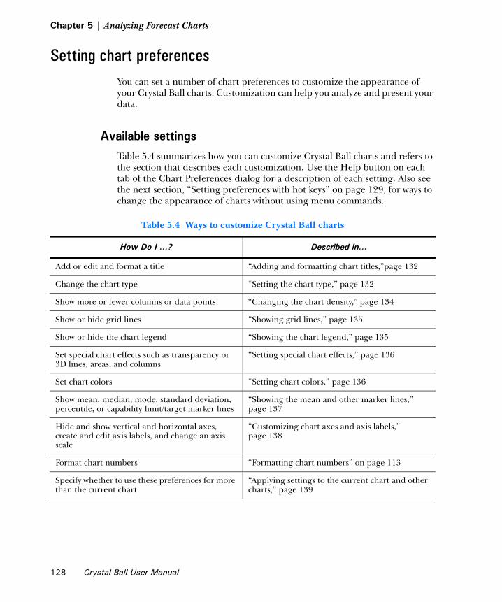
Chapter 5 | Analyzing Forecast Charts
Setting chart preferencesYou can set a number of chart preferences to customize the appearance of your Crystal Ball charts. Customization can help you analyze and present your data.
Available settingsTable 5.4 summarizes how you can customize Crystal Ball charts and refers to the section that describes each customization. Use the Help button on each tab of the Chart Preferences dialog for a description of each setting. Also see the next section, “Setting preferences with hot keys” on page 129, for ways to change the appearance of charts without using menu commands.
Table 5.4 Ways to customize Crystal Ball charts
How Do I ...? Described in...
Add or edit and format a title “Adding and formatting chart titles,”page 132
Change the chart type “Setting the chart type,” page 132
Show more or fewer columns or data points “Changing the chart density,” page 134
Show or hide grid lines “Showing grid lines,” page 135
Show or hide the chart legend “Showing the chart legend,” page 135
Set special chart effects such as transparency or 3D lines, areas, and columns
“Setting special chart effects,” page 136
Set chart colors “Setting chart colors,” page 136
Show mean, median, mode, standard deviation, percentile, or capability limit/target marker lines
“Showing the mean and other marker lines,” page 137
Hide and show vertical and horizontal axes, create and edit axis labels, and change an axis scale
“Customizing chart axes and axis labels,” page 138
Format chart numbers “Formatting chart numbers” on page 113
Specify whether to use these preferences for more than the current chart
“Applying settings to the current chart and other charts,” page 139
128 Crystal Ball User Manual

Setting chart preferences1
Setting preferences with hot keysTable 5.5 lists key combinations that can be used to cycle through settings available in the Chart Preferences dialog. Most of these commands work on the primary distribution — the probability distribution for assumptions, and frequency for forecasts and overlay charts.
Table 5.5 Hot keys for chart preferences
Hot Key Command Equivalent Description
Ctrl-d View menu; Preferences > <chartname> Preferences > View
Cycles through chart views — Frequency, Cumulative Frequency, Reverse Cumulative Frequency (for assumption and forecast charts)
Ctrl-b; Ctrl-g Preferences > Chart Preferences > General > Density
Cycles through bin or group interval values to adjust the number of columns or data points
Ctrl-l Preferences > Chart Preferences > General > Gridlines
Cycles through gridline settings: None, Horizontal, Vertical, Both
Ctrl-t Preferences > Chart Preferences > Chart Type > Type
Cycles through chart types: Area, Line, Column; for sensitivity charts: Bar (direction), Bar (magnitude), Pie (in Contribution To Variance view)
Ctrl-3 Preferences > Chart Preferences > General > 3D Chart
Cycles between two-dimensional and three-dimensional chart display
Ctrl-m Preferences > Chart Preferences > Chart Type > Marker Lines > <central tendencies>
Cycles through central tendency marker lines: None, Mean, Median, Mode (except for sensitivity and trend charts)
Ctrl-n Preferences > Chart Preferences > General > Legend
Toggles the legend display on and off
Ctrl-p Preferences > Chart Preferences > Chart Type > Marker Lines > Percentiles
Cycles through percentile marker lines: None, 10%, 20%,…90%
Spacebar View menu; Preferences > <chartname> Preferences
Cycles through window views: Chart, Statistics, Percentiles, Goodness Of Fit (if distribution fitting is selected — except for trend charts)
Crystal Ball User Manual 129

Chapter 5 | Analyzing Forecast Charts
Basic customization instructionsThese instructions apply most specifically to forecast charts. However, many of them apply to other charts as well. For that reason, they are as general as possible, although not all settings will apply to every type of chart.
To customize a chart:
1. Create or display a chart and be sure it is the active chart window.
2. Either double-click the chart or choose Preferences > Chart Preferences from the chart’s menubar.
The Chart Preferences dialog appears, similar to Figure 5.19.
Figure 5.19 The Chart Preferences dialog, General tab
3. Click each tab and make appropriate settings. Tab contents are summarized in Table 5.6. For details about the settings on each tab, click the Help button.
130 Crystal Ball User Manual

Setting chart preferences1
Overview
4. Optional step: If you want to apply the settings to more than one chart, click Apply To. Then, specify whether to apply all chart preferences or just the current tab and whether to apply them to the current Excel sheet, all sheets in the workbook, or all open and new workbooks (click the Help button for details) and click OK. Otherwise, go to step 5.
5. Click OK to apply the settings on all tabs to the active chart.
Specific customization instructionsThis section explains how you can customize each part of your Crystal Ball charts to present the information most effectively. Topics include:
• Adding and formatting chart titles, page 132
• Setting the chart type, page 132
• Changing the chart density, page 134
• Showing grid lines, page 135
• Showing the chart legend, page 135
• Setting special chart effects, page 136
• Setting chart colors, page 136
• Showing the mean and other marker lines, page 137
• Customizing chart axes and axis labels, page 138
• Applying settings to the current chart and other charts, page 139
Crystal Ball Note: For basic chart customization instructions, see page 130.
Table 5.6 Chart Preferences dialog tabs
Tab Settings
General Chart title, overall appearance of the chart
Chart Type
Data sets (series) to display in the chart, chart type and color of plotted series, marker lines to display (optional)
Axis Vertical and horizontal axes to display, axis labels, axis scales, and axis number formats
Crystal Ball User Manual 131
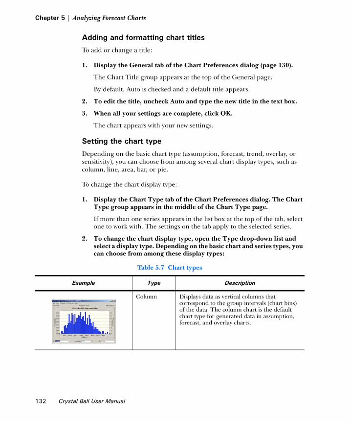
Chapter 5 | Analyzing Forecast Charts
Adding and formatting chart titles
To add or change a title:
1. Display the General tab of the Chart Preferences dialog (page 130).
The Chart Title group appears at the top of the General page.
By default, Auto is checked and a default title appears.
2. To edit the title, uncheck Auto and type the new title in the text box.
3. When all your settings are complete, click OK.
The chart appears with your new settings.
Setting the chart type
Depending on the basic chart type (assumption, forecast, trend, overlay, or sensitivity), you can choose from among several chart display types, such as column, line, area, bar, or pie.
To change the chart display type:
1. Display the Chart Type tab of the Chart Preferences dialog. The Chart Type group appears in the middle of the Chart Type page.
If more than one series appears in the list box at the top of the tab, select one to work with. The settings on the tab apply to the selected series.
2. To change the chart display type, open the Type drop-down list and select a display type. Depending on the basic chart and series types, you can choose from among these display types:
Table 5.7 Chart types
Example Type Description
Column Displays data as vertical columns that correspond to the group intervals (chart bins) of the data. The column chart is the default chart type for generated data in assumption, forecast, and overlay charts.
132 Crystal Ball User Manual

Setting chart preferences1
3. While you have a series selected, consider adjusting the chart color (page 136) and marker line settings (page 137) too.
Line Shows data as an outline of the peaks and valleys.
Area Shows data as darkened peaks and valleys.
Bar (directional)
Shows sensitivity data as horizontal bars to the right and left of the 0 line showing magnitude and direction of sensitivity
Bar (magnitude)
Shows sensitivity data as horizontal bars to the right of the 0 line showing magnitude of sensitivity but not direction
Pie Shows sensitivity data as a circle divided into proportional “slices” showing the magnitude of sensitivity
Table 5.7 Chart types (Continued)
Example Type Description
Crystal Ball User Manual 133
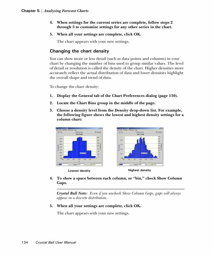
Chapter 5 | Analyzing Forecast Charts
4. When settings for the current series are complete, follow steps 2 through 3 to customize settings for any other series in the chart.
5. When all your settings are complete, click OK.
The chart appears with your new settings.
Changing the chart density
You can show more or less detail (such as data points and columns) in your chart by changing the number of bins used to group similar values. The level of detail or resolution is called the density of the chart. Higher densities more accurately reflect the actual distribution of data and lower densities highlight the overall shape and trend of data.
To change the chart density:
1. Display the General tab of the Chart Preferences dialog (page 130).
2. Locate the Chart Bins group in the middle of the page.
3. Choose a density level from the Density drop-down list. For example, the following figure shows the lowest and highest density settings for a column chart:
4. To show a space between each column, or “bin,” check Show Column Gaps.
Crystal Ball Note: Even if you uncheck Show Column Gaps, gaps will always appear in a discrete distribution.
5. When all your settings are complete, click OK.
The chart appears with your new settings.
Lowest density Highest density
134 Crystal Ball User Manual

Setting chart preferences1
Showing grid lines
Grid lines are vertical or horizontal lines that can appear on charts to help you compare the charted data with the values along the horizontal and vertical axes of the chart.
Crystal Ball Note: For basic chart customization instructions, see page 130.
To hide or show grid lines:
1. Display the General tab of the Chart Preferences dialog (page 130).
2. Locate the Options group in the middle of the page.
3. Choose a setting from the Gridlines drop-down list to show only horizontal grid lines (Horizontal), only vertical grid lines (Vertical), both horizontal and vertical grid lines (Both), or choose None to hide both horizontal and vertical grid lines.
4. When all your settings are complete, click OK.
The chart appears with the new settings.
Crystal Ball Note: You can press Ctrl-l to toggle the horizontal grid lines on and off.
Showing the chart legend
The legend shows the name and chart color for each series in the chart.
Crystal Ball Note: For basic chart customization instructions, see page 130.
To hide or show a chart legend:
1. Display the General tab of the Chart Preferences dialog (page 130).
2. Locate the Options group in the middle of the page.
3. Choose a setting from the Legend drop-down list to show the legend at the right side of the chart (Right), the left side of the chart (Left), or the bottom of the chart (Bottom). To hide the legend, choose None.
4. When all your settings are complete, click OK.
The chart appears with the new settings.
Crystal Ball Note: You can press Ctrl-n to toggle the legend on and off.
Crystal Ball User Manual 135

Chapter 5 | Analyzing Forecast Charts
Setting special chart effects
You can use special effects to help present your data most effectively. Transparency ensures that all chart series and values are visible and 3D effects add graphic depth that can be so useful when many series are charted (for example, bars become blocks as shown in the chart density figure on page 134).
Crystal Ball Note: For basic chart customization instructions, see page 130.
To set special chart effects:
1. Display the General tab of the Chart Preferences dialog (page 130).
2. Locate the Effects group at the bottom of the page.
3. You can check any or all of the available effects to see how they enhance your chart. If you check Transparency, you can also choose a percent. 0% is completely opaque and 100% is completely transparent.
4. When all your settings are complete, click OK.
The chart appears with the new settings.
Crystal Ball Note: You can press Ctrl-3 to toggle 3D display on and off.
Setting chart colors
This preference sets the color of the current chart series. This is the color that appears for the series in the chart legend, if visible.
Crystal Ball Note: For basic chart customization instructions, see page 130.
To change the chart colors:
1. Display the Chart Type tab of the Chart Preferences dialog. The Chart group appears in the middle of the Chart Type page.
If more than one series appears in the list box at the top of the tab, select one to work with. The settings on the page apply to the selected series.
2. Open the Color drop-down list and choose a color.
3. While you have a series selected, consider adjusting the chart type (page 132) and marker line settings (page 137) too.
4. When settings for the current series are complete, follow steps 2 through 3 to customize settings for any other series in the chart.
136 Crystal Ball User Manual

Setting chart preferences1
5. When all your settings are complete, click OK.
The chart appears with your new settings.
Showing the mean and other marker lines
You can display mean, mode, median, standard deviation, and other marker lines on assumption, forecast, and overlay charts. These lines help you locate various values in the charted distribution.
Crystal Ball Note: If you have activated the process capability features and have entered an LSL, USL, or Target value, you can include marker lines for them in your forecast chart. For details, see “Viewing LSL, USL, and Target marker lines” on page 347.
Base Case is the value in an assumption, decision variable, or forecast cell prior to running the simulation. For forecasts, Certainty Range shows lines at the certainty range endpoints. Marker lines are shown with labels, such as Mean = $125.
Crystal Ball Note: You can press Ctrl-m to cycle through the median, mean, and base case or mode, depending on chart type. Press Ctrl-p to cycle through every 10th percentile.
To display marker lines:
1. Display the Chart Type tab of the Chart Preferences dialog. The Marker Lines group appears in the lower right corner of the Chart Type page.
If more than one series appears in the list box at the top of the tab, select one to work with. The settings on the page apply to the selected series.
2. To display a marker line, check the box for that item. If you choose Standard Deviation, Percentile, or Value, another dialog appears:
• For Standard Deviation, enter the standard deviation(s) where you want a marker to appear. If you enter more than one, separate them with commas. Then, choose whether you want the marker(s) to appear below the mean (technically indicating negative standard deviations), above the mean, or both above and below.
• For Percentile, select the group of percentiles where you want markers to appear or choose Custom and create your own group of percentile points separated by commas.
• For Value, enter the x-axis value where the line should appear in the Value field and click Add. If you want, enter an optional label and
Crystal Ball User Manual 137

Chapter 5 | Analyzing Forecast Charts
check Show Value On Marker Line to display the value on the chart. You can click New to add another value.
3. While you have a series selected, consider adjusting the chart type (page 132) and color (page 136) too.
4. When settings for the current series are complete, follow steps 2 and 3 to customize settings for any other series in the chart.
5. When all your settings are complete, click OK.
The chart appears with your new settings.
Crystal Ball Note: If the marker lines fall outside the maximum or minimum value displayed on a chart, they will not appear on the chart. For example, this can happen with standard deviations of plus or minus 2 or 3 for uniform distributions.
Customizing chart axes and axis labels
You can customize the label, scale, and format of the main axis in Crystal Ball charts.
To customize chart axes:
1. Display the Axis tab of the Chart Preferences dialog.
2. Consider the label to use for the axis.
By default, Auto is checked in the Axis Label group. A label is automatically assigned depending on the chart type. For example, the value (x) axis of a forecast chart uses the Units entry in the Define Forecast dialog as the label. To enter a custom axis label, uncheck Auto and type a more descriptive label in the edit field.
3. Next, adjust the Scale settings. By default, Auto appears in the Type list and the chart appears with the most appropriate end points for that chart type. To use another scale, choose it from the Type drop-down list and enter the minimum (Min) and maximum (Max) values to use for the scale.
Most chart/axis combinations offer Fixed as an alternative. The value axis for assumption, forecast, and overlay charts also offers Standard Deviation and Percentile.
4. The Format Number settings control the format of the axis label numbers. Choose appropriate settings for your chart.
• For Format settings, Cell Format uses the format of the underlying cell. Most choices are similar to those used in Excel: General, Number, Currency, Scientific, Percentage, or Date.
138 Crystal Ball User Manual

Setting chart preferences1
• The Decimal settings control the number of decimal points.
• When checked, Thousand Separator inserts a thousands-separator symbol where appropriate (except when Scientific formatting is set). The thousands separator that appears is the one defined in Windows International or Regional Options settings.
Crystal Ball Note: The Format Number settings also control the format of assumption parameters in the Define Assumption dialog and assumption charts.
5. When all your settings are complete, click OK.
The chart appears with your new settings.
Applying settings to the current chart and other charts
If you would like to apply the current settings to other charts in your model, you can choose what to apply and where to apply them.
To specify how chart settings should be applied:
1. Click the Apply To button.
The Apply To dialog appears as shown in Figure 5.20.
Figure 5.20 The Apply To dialog
2. Indicate the tab or tabs of settings to apply.
• Choose This Tab to apply only settings on the current tab.
• Choose All Tabs to apply all the current settings on the entire dialog.
Crystal Ball User Manual 139

Chapter 5 | Analyzing Forecast Charts
3. Indicate where the settings should be applied.
• Choose This Sheet to apply the settings to only the current sheet of the current workbook.
• Choose This Workbook to apply the settings to all sheets of the current workbook.
• Choose All Open And New Workbooks to apply the settings to all workbooks that are currently open and all workbooks to be created.
Crystal Ball Note: The All Workbooks setting effectively changes the global Chart Preferences defaults to the settings on the current tab or all tabs, depending on the setting in the previous dialog group.
The Apply To settings are both flexible and powerful. They can be used as focused or very broad defaults.
Managing existing chartsPrevious sections of this chapter have described how to create and customize new charts. This section describes how to open, copy, paste, print, close, and delete existing charts.
Opening chartsOnce you create an assumption or forecast chart, it is saved with the workbook that contains it. Other charts are saved with the active workbook model. You can display charts again, with current data, anytime you rerun the model with associated workbooks open.
To open a chart:
1. Open the model containing the chart and run a simulation or restore saved results as described in “Restoring Crystal Ball simulation results” on page 98.
2. Open the Analyze menu and select the type of chart to display: Assumption Charts, Forecast Charts, Overlay Charts, Trend Charts, or Sensitivity Charts.
3. When the dialog for that chart appears, check the box in front of each chart you want to display.
4. Click Open.
140 Crystal Ball User Manual
Managing existing charts1
You might need to click the Crystal Ball and Microsoft Excel icons in the Windows task bar to activate charts that have disappeared behind the spreadsheet.
Crystal Ball Note: To open a number of charts at once, select the Crystal Ball data cells and choose Analyze > Open Selected Cells. All charts for the selected cells open and appear in front of any other open charts.
Copying and pasting charts to other applicationsYou can copy and paste assumption, forecast, overlay, trend, and sensitivity charts to other applications such as Microsoft Word, Powerpoint, and Excel.
Copying charts
To copy charts for use in other applications:
1. Select the chart to copy.
2. Open its View menu and choose the view to be copied.
If you choose a data view such as Percentiles, Statistics, or Goodness Of Fit, the data will be pasted into many applications as alphanumeric data, ready to edit, add, and so on. This is true for Microsoft Excel and Word, but not Powerpoint. Data is pasted into Powerpoint as a graphic.
Graphic views, such as Frequency, are pasted as bitmap images.
3. In the chart’s menubar, choose Edit > Copy.
The chart is copied to the Clipboard, ready to paste into another application.
Pasting charts from the Clipboard
To paste a chart into another application using its own Paste commands:
1. Copy the Crystal Ball chart as described in the previous section.
2. Open a document (spreadsheet, slide, and so on) in the application to receive the chart.
3. Within that application, choose Edit > Paste or Edit > Paste Special.
As described above, if you copied a data view such as Percentiles, Statistics, or Goodness of Fit, the data is pasted into many applications as editable numbers or text.
Graphic views, such as Frequency, are pasted as bitmap images.
Crystal Ball User Manual 141

Chapter 5 | Analyzing Forecast Charts
Printing chartsTo print a chart, display it and choose Edit > Print in the chart’s menubar.
Before printing, you can choose Edit > Page Setup to format the chart on the page. Then, choose Edit > Print Preview to view the chart as it will print on the selected paper size.
For example, Figure 5.21 shows the Print Preview dialog for a forecast chart from Toxic Waste Site.xls in Landscape orientation on Letter paper. Notice the block of information about the chart that appears beneath it — the chart title, the number of trials, and the certainty value for this forecast.
Figure 5.21 Print preview dialog for a forecast chart
Closing chartsWhen you close a chart, you remove it from memory but don’t delete it permanently.
To close a chart:
1. Open the Analyze menu and select the type of chart to close: Assumption Charts, Forecast Charts, Overlay Charts, Trend Charts, or Sensitivity Charts.
142 Crystal Ball User Manual

Managing existing charts1
2. When the dialog for that chart appears, check the box in front of each chart you want to close.
3. Click Close.
The selected chart or charts are closed without prompting.
Crystal Ball Note: You can use Analyze > Close All to close all chart windows from the current simulation and restored results.
Deleting chartsYou don’t need to open a chart to delete it, as long as the model or saved results file containing it is open.
To delete an overlay, trend, or sensitivity chart:
1. Open the model containing the chart.
2. Open the Analyze menu and select the type of chart to delete: Overlay Charts, Trend Charts, or Sensitivity Charts.
3. When the dialog for that chart appears, check the box in front of each chart you want to delete.
4. Click Delete.
The selected chart or charts are deleted without prompting.
Crystal Ball Note: Assumption and forecast charts cannot be deleted in this way.
Crystal Ball User Manual 143

Chapter 5 | Analyzing Forecast Charts
144 Crystal Ball User Manual

Chapter 6Analyzing Other Charts
In this chapter• Overview
• Understanding and using overlay charts
• Understanding and using trend charts
• Understanding and using sensitivity charts
• Understanding and using assumption charts
This chapter extends the information on analyzing simulation results provided in Chapter 5, “Analyzing Forecast Charts.” You will learn how to use additional charts to interpret and present data.
For information on customizing charts, managing chart windows, and printing charts, see Chapter 5.
Crystal Ball User Manual 145

Chapter 6 | Analyzing Other Charts
OverviewThe previous chapter gave guidelines for analyzing and customizing simulation results with a focus on forecast charts.
This chapter describes how to create and use a variety of additional charts:
• Overlay charts to view forecasts superimposed over each other
• Trend charts to view the certainty ranges of all your forecasts on a single chart
• Sensitivity charts to view the impact your assumptions have on forecast results
• Assumption charts to confirm random number sampling
For most effective analysis and presentation, consider this chapter as an extension of Chapter 5 and use them both together.
Understanding and using overlay chartsAfter completing a simulation with multiple related forecasts, you can create an overlay chart to view the relative characteristics of those forecasts on one chart. Then, you can compare differences or similarities that otherwise might not be apparent. There is no limit to the number of forecasts you can view at one time on an overlay chart.
For example, if a model has several forecasts based on slightly different interest rate assumptions, an overlay chart can be used to show how these slight differences manifest themselves in the variability of the forecasts. You can customize the overlay chart to accentuate these differences or similarities.
The following overlay chart shows the relative reliabilities of three manufacturing materials.
146 Crystal Ball User Manual

Understanding and using overlay charts1
Figure 6.1 An overlay chart with 3D formatting
After the simulation stops, you can also use the overlay chart to fit probability distributions to the forecasts. This process is similar to the distribution fitting feature described in Chapter 2, except that the fit is applied to forecast data, not historical data.
Creating an overlay chartThe example model used in this section, Reliability.xls, shows the reliability of a design component when it is manufactured from different materials and is subjected to varying stresses.
Each forecast chart displays the design component’s reliability as a ratio of two distributions, strength and stress. A reliable component has values greater than 1, because the component’s strength exceeds the stress subjected to it. An unreliable component has values less than 1, because its strength is less than the stress. For this model, the overlay chart can be used to compare component reliabilities.
To create an overlay chart:
1. Run a simulation in Crystal Ball.
To produce a meaningful overlay chart, the simulation should have more than one forecast. Reliability.xls is used in these instructions.
2. Choose Analyze > Overlay Charts.
Crystal Ball User Manual 147
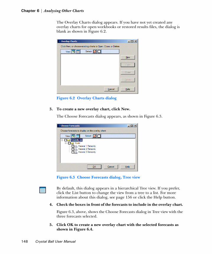
Chapter 6 | Analyzing Other Charts
The Overlay Charts dialog appears. If you have not yet created any overlay charts for open workbooks or restored results files, the dialog is blank as shown in Figure 6.2.
Figure 6.2 Overlay Charts dialog
3. To create a new overlay chart, click New.
The Choose Forecasts dialog appears, as shown in Figure 6.3.
Figure 6.3 Choose Forecasts dialog, Tree view
By default, this dialog appears in a hierarchical Tree view. If you prefer, click the List button to change the view from a tree to a list. For more information about this dialog, see page 156 or click the Help button.
4. Check the boxes in front of the forecasts to include in the overlay chart.
Figure 6.3, above, shows the Choose Forecasts dialog in Tree view with the three forecasts selected.
5. Click OK to create a new overlay chart with the selected forecasts as shown in Figure 6.4.
148 Crystal Ball User Manual

Understanding and using overlay charts1
Figure 6.4 Overlay chart for selected forecasts
The overlay chart appears with the frequency distributions for the selected forecasts superimposed over each other. By default, they are displayed as columns. You can change them to lines or areas in two or three dimensions and can change the number of data points or intervals (bins) with the Chart Preferences settings (page 128). A default name is assigned; you can also change it with the Chart Preferences settings.
6. Follow the steps in “Customizing overlay charts” on page 151 and “Setting chart preferences” beginning on page 128 to change a variety of chart features and highlight those of greatest interest.
Crystal Ball Note: You can also use “hot keys,” or keyboard equivalents for commands to quickly change the chart preferences. For a list of these, see Table 5.5 on page 129.
7. In this example, press Ctrl-d until the reverse cumulative chart view appears. Then, press Ctrl-t until the outline chart type appears.
As shown in Figure 6.5, the chart view changes to show all three distributions completely. This view in outline view most clearly suggests that Material 3 has superior reliability and is dominant since a greater proportion of its distribution is to the right of 1.00 and its values for all probability levels are higher than the others.
Legend
Menubar
Chart view
Chart title
Grid lines
y-axis title
Crystal Ball User Manual 149

Chapter 6 | Analyzing Other Charts
Figure 6.5 Overlay chart with three distributions
8. Now, experiment with chart hot keys.
Press Ctrl-d again until the frequency distribution appears. Press Ctrl-t to display the column chart. Try pressing Ctrl-b to change the number of frequency bins (columns, in this view). Then, press Ctrl-3 to make the chart three-dimensional.
Figure 6.6 Overlay chart, 3D view
150 Crystal Ball User Manual
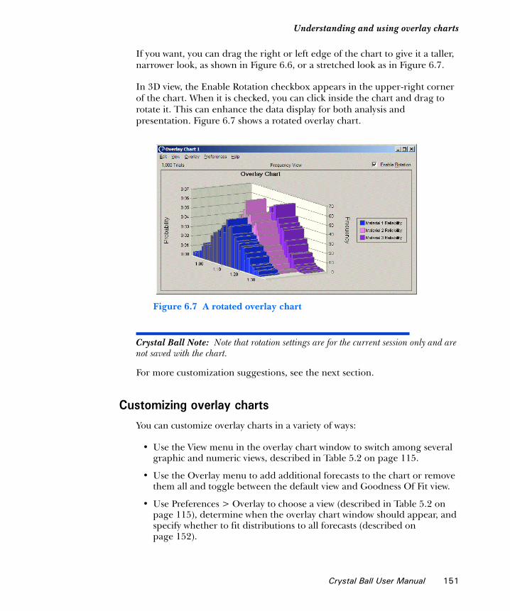
Understanding and using overlay charts1
If you want, you can drag the right or left edge of the chart to give it a taller, narrower look, as shown in Figure 6.6, or a stretched look as in Figure 6.7.
In 3D view, the Enable Rotation checkbox appears in the upper-right corner of the chart. When it is checked, you can click inside the chart and drag to rotate it. This can enhance the data display for both analysis and presentation. Figure 6.7 shows a rotated overlay chart.
Figure 6.7 A rotated overlay chart
Crystal Ball Note: Note that rotation settings are for the current session only and are not saved with the chart.
For more customization suggestions, see the next section.
Customizing overlay chartsYou can customize overlay charts in a variety of ways:
• Use the View menu in the overlay chart window to switch among several graphic and numeric views, described in Table 5.2 on page 115.
• Use the Overlay menu to add additional forecasts to the chart or remove them all and toggle between the default view and Goodness Of Fit view.
• Use Preferences > Overlay to choose a view (described in Table 5.2 on page 115), determine when the overlay chart window should appear, and specify whether to fit distributions to all forecasts (described on page 152).
Crystal Ball User Manual 151

Chapter 6 | Analyzing Other Charts
• Use Preferences > Chart Preferences to further customize the chart’s appearance as described beginning on page 128.
Customizing overlay charts helps you compare forecasts by viewing their differences in several ways. For example, the area and column chart types might obscure parts of some distributions behind other distributions, but the outline and line chart types show virtually all of each distribution. For best display of many types of data, you can choose 3D view and then rotate the chart as shown in Figure 6.7.
Using distribution fitting with overlay chartsSimilar to the distribution fitting with historical data described in “Fitting distributions to data” beginning on page 27, you can fit standard probability distributions to forecasts in an overlay chart, in addition to comparing forecasts to each other.
You can fit distributions to forecasts in overlay charts two ways:
• You can choose Overlay > Fit Probability Distributions in the overlay chart menubar to do a quick fit with the default or currently selected distributions and ranking method. You can also use this command to switch off distribution fitting that is set with either the Overlay menu or Preferences menu.
• You can choose Preferences > Overlay > Overlay Window in the overlay chart menubar to specify particular distributions and to choose one of three fit ranking methods. This way also lets you change the fit options or use Apply To to set these preferences for other overlay charts.
To fit a probability distribution to all forecasts in an overlay chart using the Preferences > Overlay command:
1. Follow the steps for forecast charts given in “Fitting a distribution to a forecast” on page 120. Wherever the instructions say Forecast, as in Preferences > Forecast, substitute Overlay.
2. Click OK to perform the fit.
Crystal Ball fits the distributions, and then displays a probability distribution for each forecast as shown in Figure 6.8.
152 Crystal Ball User Manual
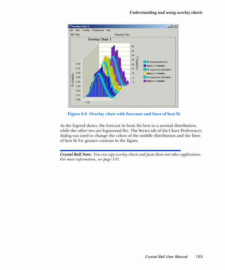
Understanding and using overlay charts1
Figure 6.8 Overlay chart with forecasts and lines of best fit
As the legend shows, the forecast in front fits best to a normal distribution, while the other two are lognormal fits. The Series tab of the Chart Preferences dialog was used to change the colors of the middle distribution and the lines of best fit for greater contrast in the figure.
Crystal Ball Note: You can copy overlay charts and paste them into other applications. For more information, see page 141.
Crystal Ball User Manual 153
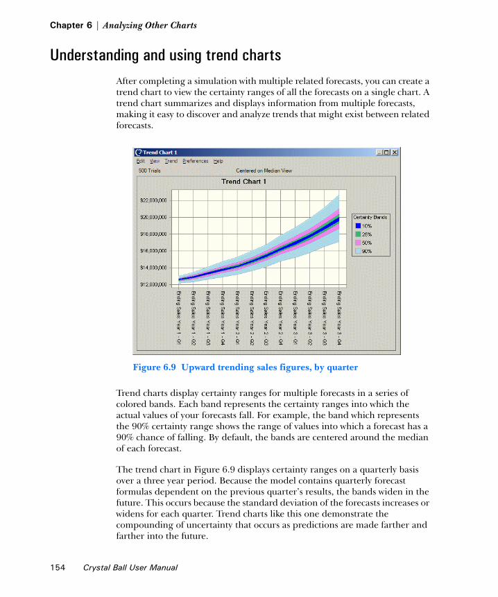
Chapter 6 | Analyzing Other Charts
Understanding and using trend chartsAfter completing a simulation with multiple related forecasts, you can create a trend chart to view the certainty ranges of all the forecasts on a single chart. A trend chart summarizes and displays information from multiple forecasts, making it easy to discover and analyze trends that might exist between related forecasts.
Figure 6.9 Upward trending sales figures, by quarter
Trend charts display certainty ranges for multiple forecasts in a series of colored bands. Each band represents the certainty ranges into which the actual values of your forecasts fall. For example, the band which represents the 90% certainty range shows the range of values into which a forecast has a 90% chance of falling. By default, the bands are centered around the median of each forecast.
The trend chart in Figure 6.9 displays certainty ranges on a quarterly basis over a three year period. Because the model contains quarterly forecast formulas dependent on the previous quarter’s results, the bands widen in the future. This occurs because the standard deviation of the forecasts increases or widens for each quarter. Trend charts like this one demonstrate the compounding of uncertainty that occurs as predictions are made farther and farther into the future.
154 Crystal Ball User Manual
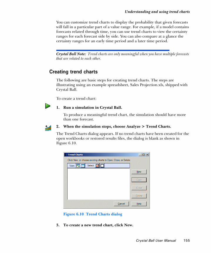
Understanding and using trend charts1
You can customize trend charts to display the probability that given forecasts will fall in a particular part of a value range. For example, if a model contains forecasts related through time, you can use trend charts to view the certainty ranges for each forecast side by side. You can also compare at a glance the certainty ranges for an early time period and a later time period.
Crystal Ball Note: Trend charts are only meaningful when you have multiple forecasts that are related to each other.
Creating trend chartsThe following are basic steps for creating trend charts. The steps are illustrating using an example spreadsheet, Sales Projection.xls, shipped with Crystal Ball.
To create a trend chart:
1. Run a simulation in Crystal Ball.
To produce a meaningful trend chart, the simulation should have more than one forecast.
2. When the simulation stops, choose Analyze > Trend Charts.
The Trend Charts dialog appears. If no trend charts have been created for the open workbooks or restored results files, the dialog is blank as shown in Figure 6.10.
Figure 6.10 Trend Charts dialog
3. To create a new trend chart, click New.
Crystal Ball User Manual 155

Chapter 6 | Analyzing Other Charts
The Choose Forecasts dialog opens, similar to Figure 6.11.
Figure 6.11 Choose Forecasts dialog for trend charts, Tree view
By default, this dialog appears in a hierarchical Tree view. If you prefer, click the List button to change to List view.
4. Select two or more forecasts to include in the trend chart.
To select a forecast, check the box in front of its name. For this example, select all forecasts in the Sales Projection worksheet. To select all forecasts in this example, you can click the Select All button or check the box in front of Sales Projection.xls or the Model tab name.
5. Click OK.
The trend chart appears as shown in Figure 6.9 on page 154.
As with overlay charts, you can change the scale and proportions of the chart by dragging its edges. For other customization possibilities, see the next section.
156 Crystal Ball User Manual
Understanding and using trend charts1
Customizing trend chartsYou can customize trend charts by:
• Changing trend chart views
• Specifying when trend charts appear
• Adding, removing, and ordering forecasts
• Changing the overall appearance of trend charts
• Setting certainty band type and colors
• Setting certainty bands
• Changing value axis preferences
The following sections describe how to make these changes.
For some of the options, you can use hot keys to bypass the Trend Preferences dialog. These hot keys are listed in Table 5.5 on page 129 and the “Menus and Keyboard Commands” chapter of the online Crystal Ball Reference Manual
Changing trend chart views
Use the trend chart View menu to change the placement of the certainty bands within the trend chart. The default setting centers the bands around the median of each forecast. You can change the location of the bands so that they are anchored at either the high end or the low end of the projected forecast ranges.
Crystal Ball Note: Smaller bands always appear on top of larger bands. This obscures the larger bands. Don’t confuse the actual width of a band with the portion that is visible. You can display the true size of a band using the certainty band preferences, described in “Setting certainty bands” on page 162. These preferences let you display the bands one at a time on the trend chart, if you wish.
To change the placement of the certainty bands:
1. In the trend chart, open the View menu.
2. Choose one of the views listed in Table 6.1, following.
Crystal Ball User Manual 157

Chapter 6 | Analyzing Other Charts
Alternately, you can choose Preferences > Trend and choose a view in the View list of the Trend Preferences dialog.
Crystal Ball Note: Use a Crystal Ball hot key to bypass the View menu. Each time you press Ctrl-d, the next trend chart view appears.
Specifying when trend charts appear
You can set preferences that determine whether the trend chart appears automatically, and if so, whether it appears while the simulation is running or after it stops.
To set these display preferences:
1. Choose Preferences > Trend.
The Trend Preferences dialog appears, as shown in Figure 6.12.
Table 6.1 Trend chart views
View Effect
Centered On Median
The default; displays forecasts centered around the median of each forecast value.
Cumulative Displays the forecasts anchored at the lower end of the forecast range; shows the certainty that the forecast values will be at or below a given value (cumulative probability).
Reverse Cumulative
Displays the forecasts anchored at the higher end of the forecast range; shows the certainty that the forecast values will be at or above a given value (reverse cumulative probability).
158 Crystal Ball User Manual

Understanding and using trend charts1
Figure 6.12 Trend Preferences dialog, Trend Window tab
2. To change the trend chart view, use the drop-down View list.
The views are discussed in the previous section, “Changing trend chart views.”
3. Use settings in the Windows group to determine whether the chart appears automatically.
If Show Automatically is checked, you can choose whether to display the chart while the simulation is running or after it stops.
4. You can click Defaults at any time to restore original default settings for the Trend Preferences dialog.
5. When all settings are complete, click OK to activate them and close the dialog.
Adding, removing, and ordering forecasts
To add and remove forecasts from a trend chart:
1. In the trend chart menubar, choose Trend > Choose Forecasts.
The Choose Forecasts dialog appears, similar to Figure 6.11 on page 156.
2. Check and uncheck forecasts to add and remove them from the chart.
Crystal Ball Note: To clear all forecast selections, choose Trend > Remove All in step 1, above.
3. Click OK to accept the settings and modify the chart.
Crystal Ball User Manual 159

Chapter 6 | Analyzing Other Charts
Once you select forecasts and create a trend chart, you can change the order that forecasts appear in the forecast axis.
To change the order of forecasts:
1. In the trend chart menubar, choose Preferences > Chart > Chart Type.
The Chart Type dialog appears, as shown in Figure 6.14 on page 161.
All charted forecasts appear in the Series list at the top of the dialog. The forecast at the top of the list appears as the first forecast at the left of the forecast axis.
2. Select a forecast in the list and use the up and down arrow keys to the right of the list to move the forecast up or down the list.
3. Optional step: You can choose Defaults at any time to restore all settings to their original default values.
4. Optional step: If you want to apply the settings to more than one chart, click Apply To. Then, specify how they should be applied (see page 139 for details) and click OK. Otherwise, go to step 5.
5. When all forecasts are positioned in order, click OK to accept the current Chart Preferences settings and modify the chart.
Changing the overall appearance of trend charts
When you first choose Preferences > Chart in the trend chart menubar, the General tab of the Chart Preferences dialog appears.
Figure 6.13 General tab, Chart Preferences dialog for trend charts
160 Crystal Ball User Manual
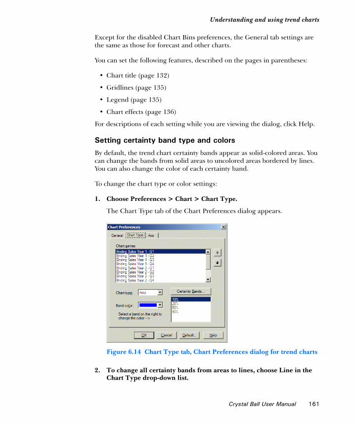
Understanding and using trend charts1
Except for the disabled Chart Bins preferences, the General tab settings are the same as those for forecast and other charts.
You can set the following features, described on the pages in parentheses:
• Chart title (page 132)
• Gridlines (page 135)
• Legend (page 135)
• Chart effects (page 136)
For descriptions of each setting while you are viewing the dialog, click Help.
Setting certainty band type and colors
By default, the trend chart certainty bands appear as solid-colored areas. You can change the bands from solid areas to uncolored areas bordered by lines. You can also change the color of each certainty band.
To change the chart type or color settings:
1. Choose Preferences > Chart > Chart Type.
The Chart Type tab of the Chart Preferences dialog appears.
Figure 6.14 Chart Type tab, Chart Preferences dialog for trend charts
2. To change all certainty bands from areas to lines, choose Line in the Chart Type drop-down list.
Crystal Ball User Manual 161

Chapter 6 | Analyzing Other Charts
3. To change the color of a certainty band:
a. Select the certainty band to change from the list below the Certainty Bands button.
b. Select a color from the Band Color list.
4. To select a different set of certainty levels or define your own, click the Certainty Bands button and follow the steps in the next section, “Setting certainty bands.”
5. Optional step: You can choose Defaults at any time to restore all settings to their original default values.
6. Optional step: If you want to apply the settings to more than one chart, click Apply To. Then, specify how they should be applied (see page 139 for details) and click OK. Otherwise, go to step 7.
7. When settings are complete, click OK to accept current settings on all tabs of the Chart Preferences dialog.
Crystal Ball Note: The Chart Series list at the top of the Chart Type tab lets you change the order of forecasts in the forecast axis. For instructions, see “Adding, removing, and ordering forecasts” on page 159.
Setting certainty bands
You can easily choose a set of certainty bands (levels) to display in the trend chart or create your own custom set.
To change or define a set of certainty bands:
1. In the trend chart menubar, choose Preferences > Chart.
2. Click the Chart Type tab, shown in Figure 6.14 on page 161.
3. On the Chart Type tab, click the Certainty Bands button.
4. The Certainty Bands dialog appears, as shown in the next figure.
162 Crystal Ball User Manual

Understanding and using trend charts1
Figure 6.15 Certainty Bands dialog
5. Choose a set of certainty bands to display on the trend chart.
6. To create your own set, choose Custom and enter a series of certainty bands, separated by commas.
7. Click OK.
The trend chart appears with the selected certainty bands. A legend appears on the right side of the trend chart indicating which levels are represented by which bands.
Crystal Ball Note: If the legend doesn’t include all bands, drag the top or the bottom of the trend chart to increase its height until all bands appear.
Changing value axis preferences
You can change several trend chart axis preferences, as described below. You can add a name for the value axis, set number formats, and set value rounding. You can also change Scale settings from Auto to Fixed and specify a range minimum and maximum value. These scale settings let you display the probability that given forecasts will fall in a particular part of a value range.
To change value axis settings:
1. In the trend chart menubar, choose Preferences > Chart > Axis.
The Axis tab of the Chart Preferences dialog appears, as shown in Figure 6.16.
Crystal Ball User Manual 163
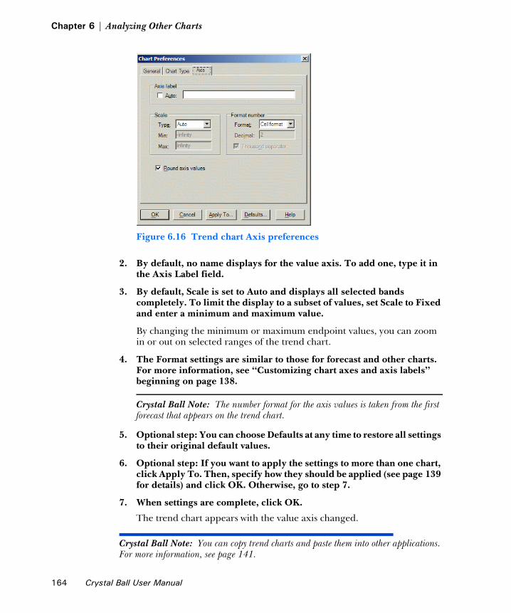
Chapter 6 | Analyzing Other Charts
Figure 6.16 Trend chart Axis preferences
2. By default, no name displays for the value axis. To add one, type it in the Axis Label field.
3. By default, Scale is set to Auto and displays all selected bands completely. To limit the display to a subset of values, set Scale to Fixed and enter a minimum and maximum value.
By changing the minimum or maximum endpoint values, you can zoom in or out on selected ranges of the trend chart.
4. The Format settings are similar to those for forecast and other charts. For more information, see “Customizing chart axes and axis labels” beginning on page 138.
Crystal Ball Note: The number format for the axis values is taken from the first forecast that appears on the trend chart.
5. Optional step: You can choose Defaults at any time to restore all settings to their original default values.
6. Optional step: If you want to apply the settings to more than one chart, click Apply To. Then, specify how they should be applied (see page 139 for details) and click OK. Otherwise, go to step 7.
7. When settings are complete, click OK.
The trend chart appears with the value axis changed.
Crystal Ball Note: You can copy trend charts and paste them into other applications. For more information, see page 141.
164 Crystal Ball User Manual

Understanding and using sensitivity charts1
Understanding and using sensitivity chartsAs you become more proficient at building spreadsheet models, you will want to know how much a given assumption affects your result. In other words, you want to determine the sensitivity of the forecast to each assumption. The overall sensitivity of a forecast to an assumption is a combination of two factors:
• The model sensitivity of the forecast to the assumption
• The assumption’s uncertainty
To determine the model sensitivity yourself, you would need to algebraically analyze the various relationships between your forecast cell and your assumption cells. These relationships include all of the formulas in the spreadsheet that link the assumption cells to the forecast cell.
Figure 6.17 illustrates two scenarios where model sensitivity and assumption uncertainty combine to affect two different forecasts. In each diagram, the distance between the assumption and the leverage point represents the model sensitivity. The larger the distance, the less model sensitivity.
Figure 6.17 Relationships between model sensitivity and assumption uncertainty
Glossary Term: sensitivity— The amount of uncertainty in a forecast cell that is caused by both the uncertainty and model sensitivity of an assumption cell.
Glossary Term: model sensitivity— The overall effect that a change in an assumption cell produces in a forecast cell. This effect is solely determined by the formulas in the spreadsheet model.
Assumption Cell Uncertainty
Assumption Cell
Leverage Point(Determined by the spreadsheet model. It represents extent to which the Assumption Cell affects the Forec
Measure of Model Sensitivity
Forecast Cell
Forecast CellUncertainty
Determined by the spreadsheet model. It represents the extent to which the assumption cell affects the forecast cell.
Measure of Model Sensitivity
Crystal Ball User Manual 165

Chapter 6 | Analyzing Other Charts
In the top model, the forecast is not as sensitive to the assumption because the model sensitivity is lower, even though there is high uncertainty in the assumption. In the bottom model, the forecast is highly sensitive to even the small assumption uncertainty because of the high model sensitivity.
Calculating these complex relationships could be a difficult and time-consuming task without a program like Crystal Ball.
About sensitivity chartsSensitivity charts show the influence each assumption cell has on a particular forecast cell. During a simulation, Crystal Ball ranks the assumptions according to their importance to each forecast cell. The sensitivity chart displays these rankings as a bar chart, indicating which assumptions are the most important or least important in the model. You can output (print) the sensitivity chart on the report or copy it to the clipboard.
Figure 6.18 Assumptions and their effects on toxicity risk
Sensitivity charts provide these key benefits:
• You can find out which assumptions are influencing your forecasts the most, reducing the amount of time needed to refine estimates.
• You can find out which assumptions are influencing your forecasts the least, so that they can be ignored or discarded altogether.
• As a result, you can construct more realistic spreadsheet models and greatly increase the accuracy of your results because you know how your assumptions affect your model.
166 Crystal Ball User Manual

Understanding and using sensitivity charts1
Creating sensitivity chartsThe example model used in this section, Toxic Waste Site.xls, illustrates the risk assessment of a toxic waste site. The sensitivity chart created in the steps below displays, in descending order, the assumptions in this model. The assumption with the highest level of sensitivity can be considered as the most influential assumption in the model.
To create a sensitivity chart:
1. Close any spreadsheets that are currently open.
2. Open the spreadsheet you want to analyze.
Toxic Waste Site.xls is used in these instructions. You can choose Help > Crystal Ball > Examples Guide to choose the model from a list.
3. Choose Run > Run Preferences > Options.
4. Make sure Store Assumption Values For Sensitivity Analysis is checked and click OK.
Sensitivity analysis requires that all of the random numbers from the simulation be kept for comparison with forecast values.
5. Run a simulation until it stops.
6. Choose Analyze> Sensitivity Charts.
The Sensitivity Charts dialog appears. If you have not yet created any sensitivity charts for the active spreadsheet or restored results file, the dialog is blank as shown in Figure 6.19.
Figure 6.19 The Sensitivity Charts dialog, blank
7. Click the New button.
Crystal Ball User Manual 167

Chapter 6 | Analyzing Other Charts
The Choose Forecast dialog appears, similar to Figure 6.20.
Figure 6.20 Choose Forecast dialog, Tree view
By default, this dialog appears in a hierarchical Tree view. If you prefer, click the List box to change the view from a tree to a list. For more information on the Choose Forecast dialog, click the Help button.
8. Check the box in front of the forecast name to include it in the sensitivity chart.
Toxic Waste.xls has only one forecast, Risk Assessment.
9. Click OK to create a new sensitivity chart as shown in Figure 6.21.
The illustrated chart has a transparency effect applied using the chart preferences to make all the numbers easier to read. For instructions, see “Setting special chart effects” beginning on page 136.
168 Crystal Ball User Manual
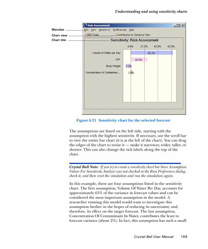
Understanding and using sensitivity charts1
Figure 6.21 Sensitivity chart for the selected forecast
The assumptions are listed on the left side, starting with the assumption with the highest sensitivity. If necessary, use the scroll bar to view the entire bar chart (it is at the left of the chart). You can drag the edges of the chart to resize it — make it narrower, wider, taller, or shorter. This can also change the tick labels along the top of the chart.
Crystal Ball Note: If you try to create a sensitivity chart but Store Assumption Values For Sensitivity Analysis was not checked in the Run Preferences dialog, check it, and then reset the simulation and run the simulation again.
In this example, there are four assumptions listed in the sensitivity chart. The first assumption, Volume Of Water Per Day, accounts for approximately 65% of the variance in forecast values and can be considered the most important assumption in the model. A researcher running this model would want to investigate this assumption further in the hopes of reducing its uncertainty and, therefore, its effect on the target forecast. The last assumption, Concentration Of Contaminant In Water, contributes the least to forecast variance (about 2%). In fact, this assumption has such a small
Menubar
Chart viewChart title
Crystal Ball User Manual 169

Chapter 6 | Analyzing Other Charts
effect, it could be ignored or altogether eliminated by clearing it from the spreadsheet.
Sensitivity charts like this one illustrate that one or two assumptions typically have a dominant effect on the uncertainty of a forecast.
How Crystal Ball calculates sensitivityCrystal Ball calculates sensitivity by computing rank correlation coefficients between every assumption and every forecast while the simulation is running. Correlation coefficients provide a meaningful measure of the degree to which assumptions and forecasts change together. If an assumption and a forecast have a high correlation coefficient, it means that the assumption has a significant impact on the forecast (both through its uncertainty and its model sensitivity). Positive coefficients indicate that an increase in the assumption is associated with an increase in the forecast. Negative coefficients imply the opposite situation. The larger the absolute value of the correlation coefficient, the stronger the relationship.
To help interpret the rank correlations, Crystal Ball provides a default chart view called the Contribution To Variance view. This view makes it easier to answer questions such as “What percentage of the variance or uncertainty in the target forecast is due to assumption X?”
It is important to note that the Contribution To Variance method is only an approximation and is not precisely a variance decomposition. Crystal Ball calculates Contribution To Variance by squaring the rank correlation coefficients and normalizing them to 100%.
Both the alternate Rank Correlation View and the Contribution To Variance view display the direction of each assumption’s relationship to the target forecast. Assumptions with a positive relationship have bars on the right side of the zero line. Assumptions with a negative relationship have bars on the left size of the zero line. If you want to show just the absolute magnitude of the relationship, you can change the Chart Type preference setting described on page 177 to Bar (Magnitude).
Crystal Ball Note: To ensure appropriate accuracy in Contribution To Variance view, consider running at least 10,000 trials.
Glossary Term: rank correlation— A method whereby assumption values are replaced with their ranking from lowest value to highest value using the integers 1 to N prior to computing the correlation coefficient.
170 Crystal Ball User Manual

Understanding and using sensitivity charts1
LimitationsSensitivity charts have several limitations you should be aware of:
• Correlated assumptions. Sensitivity calculations might be inaccurate for correlated assumptions. For example, if an important assumption were highly correlated with an unimportant one, the unimportant assumption would likely have a high sensitivity with respect to the target forecast. Assumptions that are correlated are flagged as such on the sensitivity chart. In some circumstances, turning off correlations in the Run Preferences dialog might help you to gain more accurate sensitivity information.
• Non-monotonic relationships. Sensitivity calculations might be inaccurate for assumptions whose relationships with the target forecast are not monotonic. A monotonic relationship means that an increase in the assumption tends to be accompanied by a strict increase in the forecast; or an increase in the assumption tends to be accompanied by a strict decrease in the forecast.
For example, the relationship y = Log(x) is monotonic:
While y = Sin(x) is not:
The Tornado Chart tool can help you discover if any of your assumptions have non-monotonic relationships with the target forecast. For more information, see “Tornado Chart tool” on page 211.
• Discrete distributions. Sensitivity calculations might be inaccurate for assumptions or forecasts that have a small set of discrete values. Because the sensitivity calculation relies on rank correlation, a slight loss of information occurs when the assumption or forecast values are replaced by ranks. This loss of information is generally offset by the advantage of
Crystal Ball User Manual 171

Chapter 6 | Analyzing Other Charts
being able to measure sensitivity between dissimilar types of distributions. However, when a large percentage of assumption or forecast values are very similar or identical, this loss of information grows and can significantly distort the calculation of correlations.
Be aware of this problem, for example, for:
• assumptions, when using distributions such as Binomial with a small Trials parameter (for example, < 10).
• forecasts, when formulas in your spreadsheet result in identical values (for example, if-then logic, INT functions, and so on).
Customizing sensitivity chartsYou can customize sensitivity charts by changing the assumptions, forecasts, and sensitivity preferences. As you become more familiar with the sensitivity chart, practice choosing the options that help you get the answers you seek and that are appropriate for your data.
Adding and removing assumptions
By default, the sensitivity chart includes all of the assumptions from the simulation. To remove or change the assumptions included, follow the instructions in this section.
Crystal Ball Note: The total number of assumptions included in the chart affects the calculation of the Contribution to Variance percentages. To select just which assumptions are displayed in the chart, see the text and Figure 6.24 on page 175.
To remove or change assumptions included in the sensitivity chart:
1. In the Sensitivity Chart window, choose Sensitivity > Choose Assumptions.
The Choose Assumptions dialog appears.
172 Crystal Ball User Manual
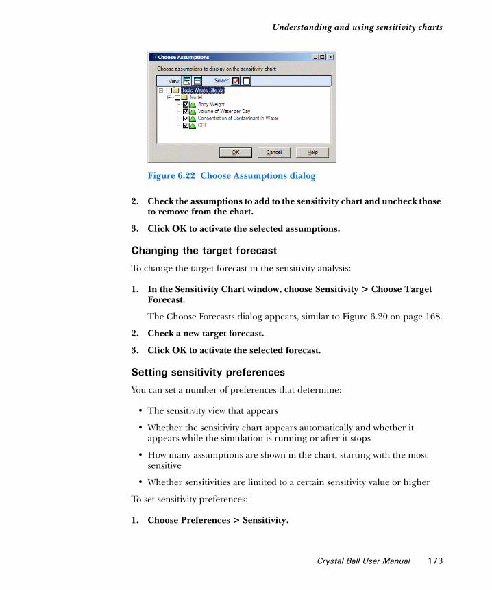
Understanding and using sensitivity charts1
Figure 6.22 Choose Assumptions dialog
2. Check the assumptions to add to the sensitivity chart and uncheck those to remove from the chart.
3. Click OK to activate the selected assumptions.
Changing the target forecast
To change the target forecast in the sensitivity analysis:
1. In the Sensitivity Chart window, choose Sensitivity > Choose Target Forecast.
The Choose Forecasts dialog appears, similar to Figure 6.20 on page 168.
2. Check a new target forecast.
3. Click OK to activate the selected forecast.
Setting sensitivity preferences
You can set a number of preferences that determine:
• The sensitivity view that appears
• Whether the sensitivity chart appears automatically and whether it appears while the simulation is running or after it stops
• How many assumptions are shown in the chart, starting with the most sensitive
• Whether sensitivities are limited to a certain sensitivity value or higher
To set sensitivity preferences:
1. Choose Preferences > Sensitivity.
Crystal Ball User Manual 173

Chapter 6 | Analyzing Other Charts
The Sensitivity Preferences dialog appears, as shown in Figure 6.23.
Figure 6.23 Sensitivity Preferences dialog, Sensitivity Window tab
2. To change how the sensitivities are presented, use the View drop-down list:
• Contribution To Variance shows sensitivities as values that range from 0% to 100% and indicate relative importance by showing the percentage of the forecast variance contributed by each assumption.
• Rank Correlation shows sensitivities as rank correlations that range from –1 to +1 and indicate both magnitude and direction of the correlation of each assumption with the forecast.
• Sensitivity Data shows a table of contributions to variance (%) and rank correlations for each assumption.
3. Use settings in the Windows group to determine whether the chart appears automatically.
If Show Automatically is checked, you can choose whether to display the chart while the simulation is running or after it stops.
4. To limit sensitivities by rank or value, click the Criteria tab to display it.
174 Crystal Ball User Manual

Understanding and using sensitivity charts1
Figure 6.24 Sensitivity Preferences dialog, Criteria tab
If you have a model with a lot of assumptions, you can check either or both boxes to limit the number of assumptions shown in the chart to a fixed number or to assumptions above a certain sensitivity value. If you check both, the more restrictive of the two criteria is used.
5. You can click Defaults at any time to restore original default settings for the Sensitivity Preferences dialog.
6. When all settings are complete, click OK to activate them and close the dialog.
Crystal Ball Note: You can copy sensitivity charts and paste them into other applications. For more information, see page 141.
Setting sensitivity chart preferences
Settings in the Sensitivity Preferences dialog determine how sensitivity is viewed and set the criteria for showing assumptions. Additional settings in the Chart Preferences dialog determine the appearance of the chart.
To set sensitivity chart preferences:
1. In the sensitivity chart window, choose Preferences > Chart.
The chart preferences dialog appears, as shown in Figure 6.25.
Crystal Ball User Manual 175

Chapter 6 | Analyzing Other Charts
Figure 6.25 Sensitivity chart Chart Preferences, General tab
2. On the General tab, you can set the following features, described on the pages in parentheses:
• Chart title (page 132)
• Gridlines (page 135)
• Legend (page 135)
• Chart effects (page 136)
Except for the disabled Chart Bins preferences, the General tab settings are the same as those for forecast charts.
For descriptions of each setting while you are viewing the dialog, click Help.
3. Click the Chart Type tab for more settings, shown in Figure 6.26.
176 Crystal Ball User Manual

Understanding and using sensitivity charts1
Figure 6.26 Sensitivity chart Chart Preferences, Chart Type tab
4. You can use the Chart Type drop-down list to choose one of these chart types:
5. For bar charts, choose whether to use a different color for each assumption (the default), or whether to use the same color for all assumptions.
Table 6.2 Sensitivity chart types
Bar (directional) The default; horizontal bars to the right and left of the 0 line showing magnitude and direction of sensitivity
Bar (magnitude) Horizontal bars to the right of the 0 line showing magnitude of sensitivity but not direction
Pie A circle divided into proportional wedges showing the magnitude of sensitivity (only available for Contribution To Variance view)
Crystal Ball User Manual 177
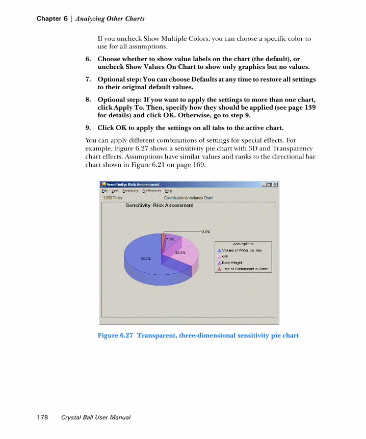
Chapter 6 | Analyzing Other Charts
If you uncheck Show Multiple Colors, you can choose a specific color to use for all assumptions.
6. Choose whether to show value labels on the chart (the default), or uncheck Show Values On Chart to show only graphics but no values.
7. Optional step: You can choose Defaults at any time to restore all settings to their original default values.
8. Optional step: If you want to apply the settings to more than one chart, click Apply To. Then, specify how they should be applied (see page 139 for details) and click OK. Otherwise, go to step 9.
9. Click OK to apply the settings on all tabs to the active chart.
You can apply different combinations of settings for special effects. For example, Figure 6.27 shows a sensitivity pie chart with 3D and Transparency chart effects. Assumptions have similar values and ranks to the directional bar chart shown in Figure 6.21 on page 169.
Figure 6.27 Transparent, three-dimensional sensitivity pie chart
178 Crystal Ball User Manual

Understanding and using assumption charts1
Understanding and using assumption chartsAssumption charts are created automatically when you run a simulation. They cannot be deleted, only opened or closed.
During or after a simulation runs, you can view assumption charts to show trial values (that is, random numbers) for the current simulation layered over the assumption’s ideal probability distribution.
Figure 6.28 Assumption chart
Assumption charts are especially useful for checking and comparing Run Preferences settings. For example, you can look at charts for the same assumption before and after increasing the number of trials and switching between Monte Carlo and Latin hypercube sampling. If certain settings yield a noticeably better match between the random numbers and the ideal distribution, you might want to use those settings even if the simulation runs longer.
Customizing assumption chartsBecause assumption charts look so similar to forecast charts, many of their menu commands and settings are the same.
Crystal Ball User Manual 179

Chapter 6 | Analyzing Other Charts
Setting assumption chart views
You can use the View menu to choose five views: Probability, Cumulative Probability, Reverse Cumulative Probability, Statistics, and Percentiles. For a description of these views and how to select them, see “Changing the distribution view and interpreting statistics” beginning on page 115.
Setting assumption preferences
Assumption preferences, set with Preferences > Assumptions, are similar to those for forecasts, described in “Setting forecast preferences” beginning on page 125. By default, assumption charts are not shown when you run a simulation. You can change the Show Automatically setting to automatically show assumption charts while a simulation is running or when it stops.
Figure 6.29 Assumption Preferences dialog
While the Forecast Preferences dialog has a button for fitting distributions to forecasts, distribution fitting isn’t available in the Assumption Preferences dialog. Instead, there is a Run Preferences button so you can easily change the Store Assumption Values... setting on the Options tab of the Run Preferences dialog. For more information on the Assumption Preferences dialog, click the Help button in the dialog.
Setting assumption chart preferences
Assumption chart preferences are virtually identical to forecast chart preferences. To review or change them, choose Preferences > Chart and follow the instructions beginning on page 128.
180 Crystal Ball User Manual

Chapter 7Creating Reports and Extracting Data
In this chapter• Creating reports
• Extracting data
This chapter describes how to create reports with charts and data and how to extract data for use in other applications.
Crystal Ball User Manual 181

Chapter 7 | Creating Reports and Extracting Data
Creating reportsYou can generate pre-defined reports for your simulation or you can create a custom report with any or all of the following items:
• Report summary
• Forecasts
• Assumptions
• Decision variables
• Overlay charts
• Trend charts
• Sensitivity charts
Figure 7.1 shows part of a forecast report for the Vision Research model.
Figure 7.1 Sample forecast report
182 Crystal Ball User Manual

Creating reports1
Basic steps
Crystal Ball Note: If ### appears in your report instead of a numeric value, try making the column wider to show the entire number.
To create a report:
1. Choose Analyze > Create Report.
The Create Report Preferences dialog appears, as in Figure 7.2.
Figure 7.2 Create Report dialog, Reports tab
2. Click an icon to choose a report.
You can choose one of five pre-defined reports or click the Custom button to define your own. The choices are as follows:
• Assumptions — report summary plus assumption parameters, charts, and correlations.
• Decision Variables — decision variable bounds, variable types, and step size (if discrete).
• Forecasts — report summary plus forecast summaries, charts, statistics, percentiles, and capability metrics if generated.
• Full, the default — all sections and details except assumption statistics and percentiles.
• Index — only forecast, assumption, and decision variable summaries.
Crystal Ball User Manual 183
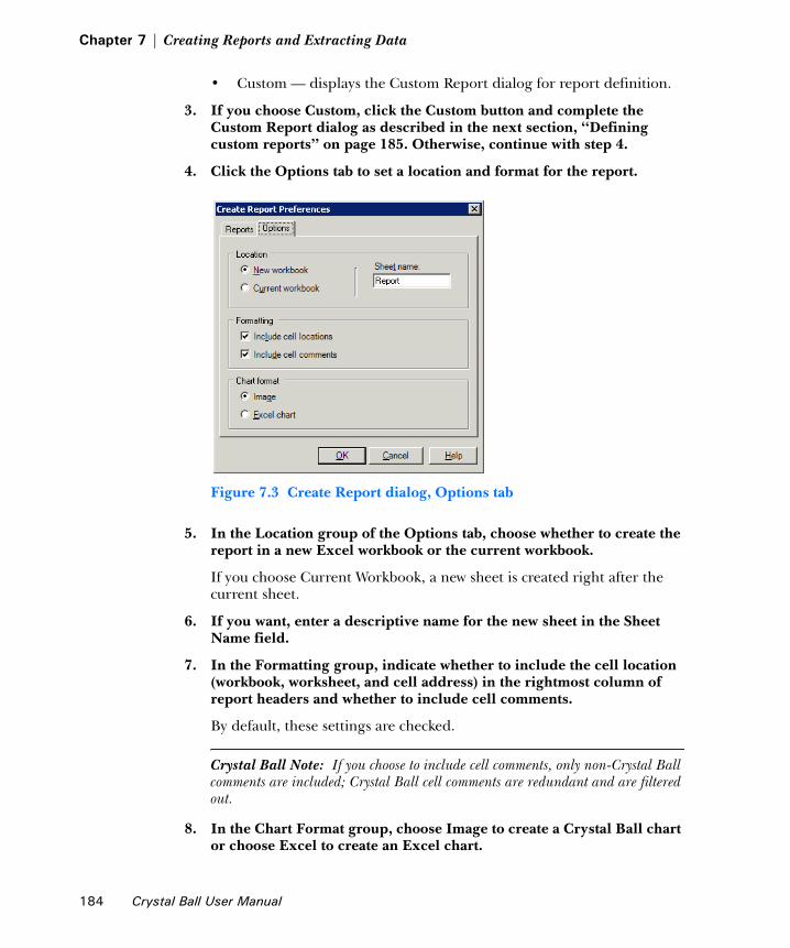
Chapter 7 | Creating Reports and Extracting Data
• Custom — displays the Custom Report dialog for report definition.
3. If you choose Custom, click the Custom button and complete the Custom Report dialog as described in the next section, “Defining custom reports” on page 185. Otherwise, continue with step 4.
4. Click the Options tab to set a location and format for the report.
Figure 7.3 Create Report dialog, Options tab
5. In the Location group of the Options tab, choose whether to create the report in a new Excel workbook or the current workbook.
If you choose Current Workbook, a new sheet is created right after the current sheet.
6. If you want, enter a descriptive name for the new sheet in the Sheet Name field.
7. In the Formatting group, indicate whether to include the cell location (workbook, worksheet, and cell address) in the rightmost column of report headers and whether to include cell comments.
By default, these settings are checked.
Crystal Ball Note: If you choose to include cell comments, only non-Crystal Ball comments are included; Crystal Ball cell comments are redundant and are filtered out.
8. In the Chart Format group, choose Image to create a Crystal Ball chart or choose Excel to create an Excel chart.
184 Crystal Ball User Manual
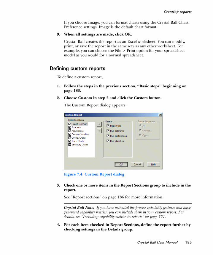
Creating reports1
If you choose Image, you can format charts using the Crystal Ball Chart Preference settings. Image is the default chart format.
9. When all settings are made, click OK.
Crystal Ball creates the report as an Excel worksheet. You can modify, print, or save the report in the same way as any other worksheet. For example, you can choose the File > Print option for your spreadsheet model as you would for a normal spreadsheet.
Defining custom reportsTo define a custom report,
1. Follow the steps in the previous section, “Basic steps” beginning on page 183.
2. Choose Custom in step 2 and click the Custom button.
The Custom Report dialog appears.
Figure 7.4 Custom Report dialog
3. Check one or more items in the Report Sections group to include in the report.
See “Report sections” on page 186 for more information.
Crystal Ball Note: If you have activated the process capability features and have generated capability metrics, you can include them in your custom report. For details, see “Including capability metrics in reports” on page 351.
4. For each item checked in Report Sections, define the report further by checking settings in the Details group.
Crystal Ball User Manual 185

Chapter 7 | Creating Reports and Extracting Data
As each item is highlighted in the Report Sections group, appropriate settings appear in the Details group. For descriptions of these, see “Report details” beginning on page 187.
5. For each item checked in Report Sections, choose whether to display all of that type of item, only selected items, or all open items.
As each item is highlighted in the Report Sections group, appropriate display settings appear in the group at the upper right of the dialog. This group is labeled with the name of the current selection in the Report Sections group. If you choose Choose, a dialog appears so you can check the box in front of each item to display.
6. When these settings are complete, click OK to close the dialog and return to the Create Report dialog.
7. In the Create Report dialog, click the Options tab to display it and continue with step 5 on page 184.
8. When all the report options are set, click OK to close the dialog and create the report.
Report sections
The Crystal Ball Custom report offers the following sections. You can include any or all of them.
Figure 7.5 Custom report sections
Table 7.1 Create Report dialog, Report Sections settings
Setting Effect
Report Summary Includes the report title, date and time, Run Preferences settings, and run statistics.
Forecasts Includes various types of forecast information, including the name, charts, percentiles, statistics, and more.
Assumptions Includes various types of assumption information, including parameters, charts, percentiles, statistics, and correlations.
186 Crystal Ball User Manual

Creating reports1
Crystal Ball Note: Excel charts cannot be created for assumptions defined as custom distributions.
Report details
The Crystal Ball Custom report offers details for each section. Within a section, you can include any or all of them. The details are described in Table 7.2.
Some of the Details settings display chooser dialogs. For more information about these, click Help in the dialog.
Decision Variables Includes various types of decision variable information, including type (continuous or discrete) with step if discrete, plus lower and upper bounds.
Overlay Charts Includes overlay charts in the report. You can scale the size of the charts by entering a percentage in the field.
Trend Charts Includes trend charts in the report. You can scale the size of the charts by entering a percentage in the field.
Sensitivity Charts Includes sensitivity charts in the report. You can scale the size of the charts by entering a percentage in the field.
Table 7.1 Create Report dialog, Report Sections settings (Continued)
Setting Effect
Crystal Ball User Manual 187

Chapter 7 | Creating Reports and Extracting Data
Table 7.2 Custom report sections and details
Section Detail Description
Report Summary Report Title Name of the report; default is “Crystal Ball Report.”
Date/Time Date and time when the simulation included in the report was started and stopped.
Run Preferences Run Preferences settings for the report:• Number of trials run = X,XXX
• Monte Carlo sampling or Latin Hypercube sampling (Latin Hypercube sample size)
• Random seed or Seed = XXX
• Precision Control on (if true)
• Correlations disabled (only if disabled)
• User macros disabled (only if disabled)
Run Statistics First section is an exact duplicate of the Control Panel Statistics tab with frozen items = X,XXX (at the end, if items were frozen)Second section is as follows:User macros executed<workbook1!sheet1>CBBeforeSimulation<workbook1!sheet1>CBAfterTrialetc…
Forecasts Summary
Chart And Size Default = 100% for all charts.
Statistics
Percentiles Selected in the Percentiles dialog; the default is Deciles.
Assumptions Parameters Lists the parameters used to define the distribution.
Chart And Size Default = 50% for all charts.
Statistics Theoretical and empirical (if saved during the simulation)
Percentiles Selected in the Percentiles dialog; the default is Deciles.
Correlations
188 Crystal Ball User Manual

Creating reports1
Crystal Ball Note: When no details are selected for a custom report section, only a single row is output with the Crystal Ball item name and the cell reference.
Report processing notes
The following are special notes concerning Crystal Ball reports:
• No section is created if there are no Crystal Ball items for that section.
• Statistics follow the chart by default.
• The Choose > All options always include restored results if they exist.
• If scroll bars are present in a chart, they appear in the report.
• If an assumption has been truncated, you might want to add marker lines to show where the distribution has been truncated. To do this, display the Chart Type tab in the Chart Preferences dialog and set an appropriate Value marker.
Decision Variables Type Continuous or Discrete; Step Size
Bounds
Overlay Charts Chart And Size Default = 100% for all charts.
Trend Charts Chart And Size Default = 100% for all charts.
Sensitivity Charts Chart And Size Default = 100% for all charts.
Table 7.2 Custom report sections and details (Continued)
Section Detail Description
Crystal Ball User Manual 189

Chapter 7 | Creating Reports and Extracting Data
Extracting dataCrystal Ball lets you extract assumption and forecast information generated during a simulation. Crystal Ball places the extracted data in a worksheet location you select. You can only extract data after you run a simulation or restore saved results.
To extract data:
1. Choose Analyze > Extract Data.
The Extract Data dialog appears, as in Figure 7.6.
Figure 7.6 Extract Data dialog, Data tab
2. To select the type of data to extract, choose the appropriate setting in the Select Data To Extract list, described in Table 7.3.
Table 7.3 Extract Data dialog, Select Data To Extract settings
Option Extracts...
Statistics Descriptive statistics summarizing the assumption and forecast values.
Percentiles The probability of achieving values below a particular threshold in the selected increments.
Note: You can reverse the meaning of the percentiles by changing the setting in the Run Preferences > Options dialog. For more information, see “Statistics preferences” on page 87.
190 Crystal Ball User Manual
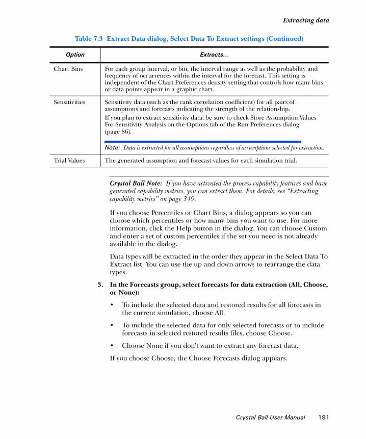
Extracting data1
Crystal Ball Note: If you have activated the process capability features and have generated capability metrics, you can extract them. For details, see “Extracting capability metrics” on page 349.
If you choose Percentiles or Chart Bins, a dialog appears so you can choose which percentiles or how many bins you want to use. For more information, click the Help button in the dialog. You can choose Custom and enter a set of custom percentiles if the set you need is not already available in the dialog.
Data types will be extracted in the order they appear in the Select Data To Extract list. You can use the up and down arrows to rearrange the data types.
3. In the Forecasts group, select forecasts for data extraction (All, Choose, or None):
• To include the selected data and restored results for all forecasts in the current simulation, choose All.
• To include the selected data for only selected forecasts or to include forecasts in selected restored results files, choose Choose.
• Choose None if you don’t want to extract any forecast data.
If you choose Choose, the Choose Forecasts dialog appears.
Chart Bins For each group interval, or bin, the interval range as well as the probability and frequency of occurrences within the interval for the forecast. This setting is independent of the Chart Preferences density setting that controls how many bins or data points appear in a graphic chart.
Sensitivities Sensitivity data (such as the rank correlation coefficient) for all pairs of assumptions and forecasts indicating the strength of the relationship.If you plan to extract sensitivity data, be sure to check Store Assumption Values For Sensitivity Analysis on the Options tab of the Run Preferences dialog (page 86).
Note: Data is extracted for all assumptions regardless of assumptions selected for extraction.
Trial Values The generated assumption and forecast values for each simulation trial.
Table 7.3 Extract Data dialog, Select Data To Extract settings (Continued)
Option Extracts...
Crystal Ball User Manual 191
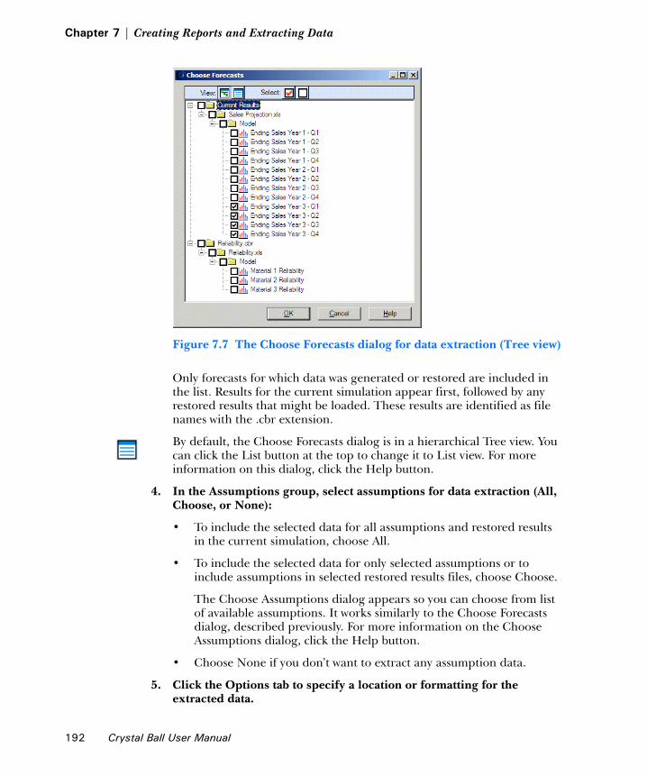
Chapter 7 | Creating Reports and Extracting Data
Figure 7.7 The Choose Forecasts dialog for data extraction (Tree view)
Only forecasts for which data was generated or restored are included in the list. Results for the current simulation appear first, followed by any restored results that might be loaded. These results are identified as file names with the .cbr extension.
By default, the Choose Forecasts dialog is in a hierarchical Tree view. You can click the List button at the top to change it to List view. For more information on this dialog, click the Help button.
4. In the Assumptions group, select assumptions for data extraction (All, Choose, or None):
• To include the selected data for all assumptions and restored results in the current simulation, choose All.
• To include the selected data for only selected assumptions or to include assumptions in selected restored results files, choose Choose.
The Choose Assumptions dialog appears so you can choose from list of available assumptions. It works similarly to the Choose Forecasts dialog, described previously. For more information on the Choose Assumptions dialog, click the Help button.
• Choose None if you don’t want to extract any assumption data.
5. Click the Options tab to specify a location or formatting for the extracted data.
192 Crystal Ball User Manual

Extracting data1
Figure 7.8 Extract Data dialog, Options tab
6. In the Location area:
• To extract data to a new workbook, choose New Workbook.
• To extract data to a new worksheet in the active workbook, choose Current Workbook > New Sheet.
• To extract data to the current sheet, choose Current Workbook > Current Sheet.
7. Specify the name of the sheet and the first cell of the range where the extracted data will be stored.
8. Check settings in the Formatting group to indicate how you want to format the extracted data:
• When checked, Include Labels adds row and column headers to the data table. Otherwise, just the numeric values are extracted.
• When checked, Include Cell Locations adds the workbook, worksheet, and cell address above the object name in the column header. Otherwise, only the object name appears.
Cell Location labels
Crystal Ball User Manual 193

Chapter 7 | Creating Reports and Extracting Data
• When checked, AutoFormat applies the following formats to extracted data:
Bold font for column headers Border beside row labels Border beneath column headers Border before first assumption Numeric formatting to values AutoFit width to columns
9. If you want, you can click the Defaults button at any time to restore the original settings to both tabs of the Extract Data dialog.
10. When both the Data and Options tab settings are complete, click OK.
Crystal Ball extracts the simulation data to the specified worksheet location. The extracted data is arranged as columns of forecasts and assumptions and rows of data. You can sort, modify, print, or save the data in the same way as any other spreadsheet.
The following figures show samples of different types of data extracted with all Formatting settings checked (forecasts only).
Figure 7.9 A sample of extracted data, Statistics format
194 Crystal Ball User Manual
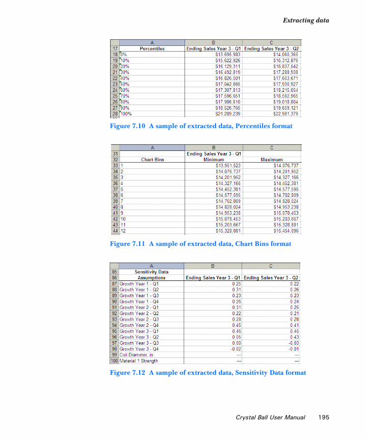
Extracting data1
Figure 7.10 A sample of extracted data, Percentiles format
Figure 7.11 A sample of extracted data, Chart Bins format
Figure 7.12 A sample of extracted data, Sensitivity Data format
Crystal Ball User Manual 195

Chapter 7 | Creating Reports and Extracting Data
Figure 7.13 A sample of extracted data, Trial Values format
196 Crystal Ball User Manual

Chapter 8Crystal Ball Tools
In this chapterThis chapter describes the Crystal Ball tools:
• Batch Fit tool
• Correlation Matrix tool
• Tornado Chart tool
• Bootstrap tool
• Decision Table tool
• Scenario Analysis tool
• Two-Dimensional Simulation tool
For each tool, there is a general description, an introduction tutorial, and references to descriptions of all dialogs, fields, and options.
Crystal Ball User Manual 197

Chapter 8 | Crystal Ball Tools
OverviewCrystal Ball tools are Visual Basic programs in the Run > Tools menu that extend the functionality of Crystal Ball. They cover two aspects of Crystal Ball modeling: setup and analysis.
This chapter describes each tool and provides a step-by-step example for using it.
CB Tools Note: Some of the tools can take a long time to run. Should you need to cancel a tool before it stops by itself, click in the Excel window and hit Esc. A dialog will appear and you can choose to End or Continue.
Table 8.1 Setup tools
Tool Action
Batch Fit Automatically fits selected continuous probability distributions to multiple data series.
Correlation Matrix Rapidly defines and automates correlations of assumptions.
Tornado Chart Individually analyzes the impact of each model variable on a target outcome.
Table 8.2 Analysis tools
Tool Action
Bootstrap Addresses the reliability and accuracy of forecast statistics.
Decision Table Evaluates the effects of alternate decisions in a simulation model.
Scenario Analysis Displays what inputs created particular outputs.
Two-Dimensional Simulation Independently addresses uncertainty and variability using a two-dimensional simulation.
198 Crystal Ball User Manual

Batch Fit tool1
Batch Fit toolThe Batch Fit tool fits probability distributions to multiple data series. You can select any or all of the continuous probability distributions (normal, triangular, uniform, etc.) to fit to any number of series limited only by the size of your spreadsheet.
Batch Fit is intended to help you create assumptions when you have historical data for several variables. It selects which distribution best fits each series of historical data, and gives you the distribution and its associated parameters for you to use in your model. This tool also gives you a table of goodness-of-fit statistics for the best fitting distribution and provides a matrix of correlations calculated between multiple data series so you can easily see which series are related and to what degree.
To use the Batch Fit tool, your data series must be contiguous (in adjacent rows or columns) in either rows or columns.
You can select any combination of the continuous probability distributions to fit to all your data series.
Batch Fit exampleIn the Crystal Ball Examples folder, there is a Magazine Sales.xls spreadsheet you can use to experiment with the Batch Fit tool. This spreadsheet model shows the estimated gross profit resulting from newsstand sales of four of the company’s most popular magazines.
Figure 8.1 Magazine Sales workbook
Crystal Ball User Manual 199

Chapter 8 | Crystal Ball Tools
In this model, cells C5 through F5 are formulas that refer to the first row of data on the Sales Data worksheet. However, the model would be more accurate if you replaced these formulas with assumptions based on historical data. To do this, you can use the Batch Fit tool to generate an assumption for each data column of the Sales Data worksheet. Then, you can use Crystal Ball commands to copy and paste those assumptions from the Batch Fit data to the first data row of the Magazine Sales model. Because Crystal Ball cannot define assumptions in formula cells, you need to convert the formulas in C5 to F5 to values before pasting the assumption cells.
Generating Batch Fit results
To run the Batch Fit tool:
1. In Excel with Crystal Ball loaded, open the workbook Magazine Sales.xls.
2. Select Run > Tools > Batch Fit.
The Select Distributions dialog appears, as shown in Figure 8.2
Figure 8.2 Select Distributions dialog, Batch Fit tool
3. Make sure all the distributions are in the Selected Distributions list.
4. Click Next.
The Select Input Options dialog appears, as shown in Figure 8.3 (with data filled in from steps 5 through 11).
200 Crystal Ball User Manual

Batch Fit tool1
Figure 8.3 Select Input Options dialog, Batch Fit tool
5. Click the Select Cells icon to the right of the Location Of Data Series field.
6. Select the Sales Data worksheet.
7. Select cells A1 through D361.
8. Click the Return icon to return to the Batch Fit dialog.
9. Select Data In Columns, the default.
10. Check the First Row Contains Headers option.
11. Select the Ranking Method: Chi-Square.
12. Click Next.
The Select Output Options dialog appears.
Crystal Ball User Manual 201

Chapter 8 | Crystal Ball Tools
Figure 8.4 Select Output Options dialog, Batch Fit tool
13. Select the Create Output On The Active Worksheet option.
14. Click the Select Cells icon to the right of the Specify Upper Left Corner Of The Output field.
15. Select the Sales Model tab.
16. Select cell B13.
17. Click the return icon to return to the Batch Fit dialog.
18. Make sure the Format Output option is checked.
19. Set the Output Orientation to Data In Columns.
20. Check the Show Table Of Goodness-of-fit Statistics option.
21. To include a correlation analysis of the data:
a. Check the Calculate Correlations Between Series option.
b. Enter a threshold value in the Define Correlations Above field.
The threshold must be between 0 and 1 (inclusive). The tool displays the correlation matrix at the end of the results section.
22. Click Start.
The tool fits each selected distribution to each data series. The results appear on the Sales Model worksheet below the existing table, similar to Figure 8.5.
202 Crystal Ball User Manual

Batch Fit tool1
Figure 8.5 Batch Fit results below the model
Using Batch Fit results in a model
Now that assumptions have been generated from historic sales data, the next steps are to convert Sales Volume formulas to values and replace them with the new assumptions. Then, you can run a simulation with more accurate results.
To use Batch Fit results in a model:
1. Select the formulas in cells C5 through F5.
2. Use Excel’s Copy and Paste Special commands to copy the formula cells and paste them back into the same locations. When the Paste Special dialog appears, choose Values as the Paste setting. Leave the other default settings and click OK.
3. Copy assumption data into the worksheet.
a. Select cells C15 through F15.
b. Select Define > Copy Data.
Notice this is Crystal Ball’s Copy Data command, not Excel’s Copy command.
Crystal Ball Note: This function copies Crystal Ball data only, not the cell value.
Crystal Ball User Manual 203
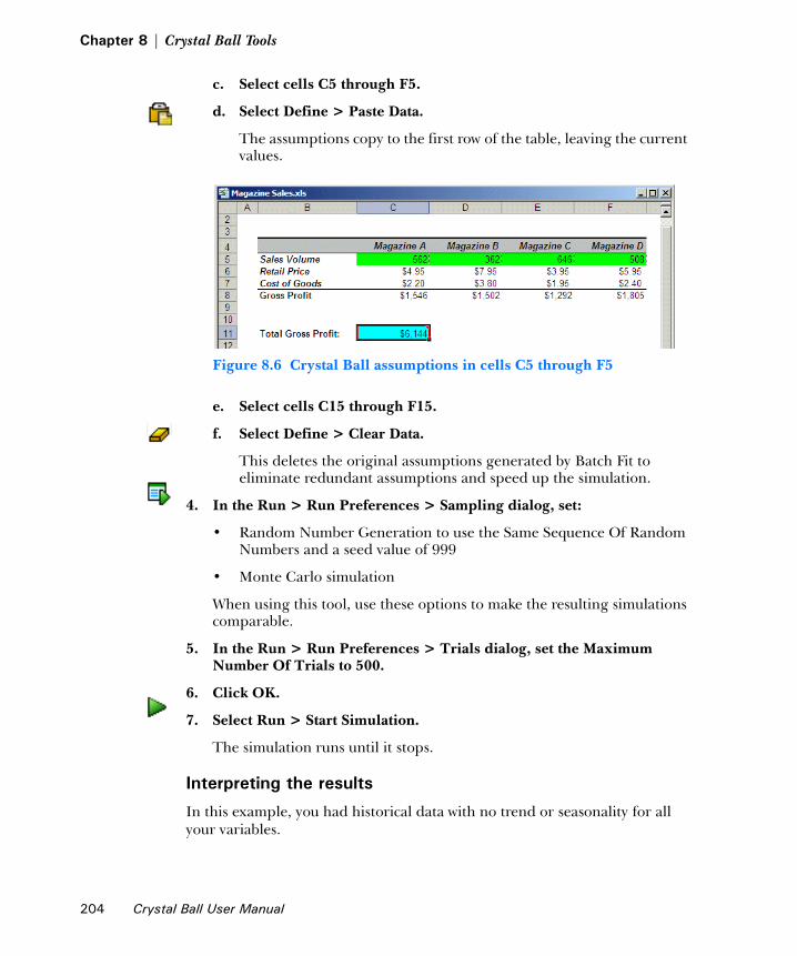
Chapter 8 | Crystal Ball Tools
c. Select cells C5 through F5.
d. Select Define > Paste Data.
The assumptions copy to the first row of the table, leaving the current values.
Figure 8.6 Crystal Ball assumptions in cells C5 through F5
e. Select cells C15 through F15.
f. Select Define > Clear Data.
This deletes the original assumptions generated by Batch Fit to eliminate redundant assumptions and speed up the simulation.
4. In the Run > Run Preferences > Sampling dialog, set:
• Random Number Generation to use the Same Sequence Of Random Numbers and a seed value of 999
• Monte Carlo simulation
When using this tool, use these options to make the resulting simulations comparable.
5. In the Run > Run Preferences > Trials dialog, set the Maximum Number Of Trials to 500.
6. Click OK.
7. Select Run > Start Simulation.
The simulation runs until it stops.
Interpreting the results
In this example, you had historical data with no trend or seasonality for all your variables.
204 Crystal Ball User Manual

Batch Fit tool1
Crystal Ball Note: If your historical data have a time-series element, trend, or seasonality, you should use CB Predictor instead of the distribution fitting functionality. CB Predictor is a component of Crystal Ball Professional and Premium Editions.
When the Batch Fit tool runs, it fits each column of data to each continuous distribution. For each fit of a distribution to a set of data, the tool calculates the indicated goodness-of-fit test. The distribution with the best fit is placed in the spreadsheet to create an assumption cell that you can copy to the appropriate location in your model.
In this example, the four columns of data resulted in four assumptions that you copied to the appropriate locations. The forecast is already defined for you, and running a simulation produces a forecast chart of the total gross profit from the Magazine Sales workbook. In the Total Gross Profit forecast chart, if you replace –Infinity with $5,500, you find that the certainty or probability of making this amount of profit is almost 75%.
Figure 8.7 Magazine Sales profit from newsstand sales
Crystal Ball User Manual 205

Chapter 8 | Crystal Ball Tools
Correlation Matrix tool
CorrelationsWhen the values of two variables depend on each other in any way, you should correlate them to increase the accuracy of your simulation's forecast results.
There are two types of correlations:
The correlation coefficient range is -1 to 1, where 0 indicates no correlation. The closer the coefficient is to ±1, the stronger the relationship between the assumptions. You should never use a coefficient of ±1; represent relationships this closely correlated with formulas in the spreadsheet model.
Correlation matrixIn Crystal Ball, you enter correlations one at a time using the Correlation dialog. Instead of manually entering the correlations this way, you can use the Correlation Matrix tool to define a matrix of correlations between assumptions in one simple step. This saves time and effort when building your spreadsheet model, especially for models with many correlated assumptions.
The correlation matrix is either an upper or lower triangular matrix with ones along the diagonal. When entering coefficients, think of the matrix as a multiplication table. If you follow one assumption along its horizontal row and the second along its vertical column, the value in the cell where they meet is their correlation coefficient. The matrix contains only the correlation coefficients you enter.
Table 8.3 Types of correlations
positive correlation Indicates that two assumptions increase or decrease together. For example, the price of gasoline and shipping costs increase and decrease together.
negative correlation Indicates that an increase in one assumption results in a decrease in the other assumption. For example, the more items you buy from a particular vendor, the lower the unit cost.
206 Crystal Ball User Manual
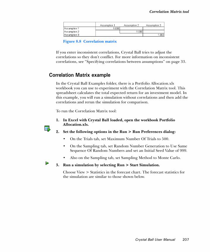
Correlation Matrix tool1
Figure 8.8 Correlation matrix
If you enter inconsistent correlations, Crystal Ball tries to adjust the correlations so they don’t conflict. For more information on inconsistent correlations, see “Specifying correlations between assumptions” on page 33.
Correlation Matrix exampleIn the Crystal Ball Examples folder, there is a Portfolio Allocation.xls workbook you can use to experiment with the Correlation Matrix tool. This spreadsheet calculates the total expected return for an investment model. In this example, you will run a simulation without correlations and then add the correlations and rerun the simulation for comparison.
To run the Correlation Matrix tool:
1. In Excel with Crystal Ball loaded, open the workbook Portfolio Allocation.xls.
2. Set the following options in the Run > Run Preferences dialog:
• On the Trials tab, set Maximum Number Of Trials to 500.
• On the Sampling tab, set Random Number Generation to Use Same Sequence Of Random Numbers and set an Initial Seed Value of 999.
• Also on the Sampling tab, set Sampling Method to Monte Carlo.
3. Run a simulation by selecting Run > Start Simulation.
Choose View > Statistics in the forecast chart. The forecast statistics for the simulation are similar to those shown below.
Crystal Ball User Manual 207

Chapter 8 | Crystal Ball Tools
Figure 8.9 Uncorrelated simulation statistics
4. Choose Run > Reset to reset the simulation.
5. Select Run > Tools > Correlation Matrix.
The Select Assumptions dialog appears as shown in Figure 8.10.
Figure 8.10 Select Assumptions dialog, Correlation Matrix tool
6. Include all the assumptions in the correlation matrix by moving all the assumptions from the Available Assumptions list to the Selected Assumptions list by either:
• Double-clicking on each assumption to move.
208 Crystal Ball User Manual

Correlation Matrix tool1
• Selecting each assumption to move and clicking on >> to move it.
• Making an extended selection using the Shift or Ctrl keys.
7. Click Next.
The Specify Options dialog appears.
Figure 8.11 Specify Options dialog, Correlation Matrix tool
8. Choose the following settings:
• Create A Temporary Correlation Matrix On A New Worksheet
• Upper Triangular Matrix
9. Click Start.
The tool creates a temporary matrix in a new workbook.
10. Enter the following correlation coefficients into the matrix.
Crystal Ball User Manual 209

Chapter 8 | Crystal Ball Tools
CB Tools Note: Leaving a cell blank is not the same as entering a zero. Values that are not specified in the matrix will be filled in with estimates of appropriate values when the simulation runs.
11. Click Load The Matrix.
The tool loads the correlation coefficients from the matrix into your Crystal Ball model. Loading a full correlation matrix for all assumptions can take several minutes or even longer.
CB Tools Note: If a Matrix Successfully Loaded message doesn’t appear, press Tab or Return to exit the current cell and then click Load The Matrix again.
12. Reset the simulation.
13. Rerun the simulation.
The forecast statistics for the correlated simulation are shown in Figure 8.12.
Figure 8.12 Correlated simulation statistics
210 Crystal Ball User Manual
Tornado Chart tool1
The standard deviation is now much higher than the original simulation due to the correlations. The original model without the correlations ignored this risk factor and its effects.
CB Tools Note: For details on the Correlation Matrix dialogs and their settings, click Help in a dialog.
Tornado Chart toolThe Tornado Chart tool measures the impact of each model variable one at a time on a target forecast. The tool displays the results in two ways:
• Tornado chart
• Spider chart
This method differs from the correlation-based method built into Crystal Ball in that this tool tests each assumption, decision variable, precedent, or cell independently. While analyzing one variable, the tool freezes the other variables at their base values. This measures the effect of each variable on the forecast cell while removing the effects of the other variables. This method is also known as “one-at-a-time perturbation” or “parametric analysis.”
The Tornado Chart tool is useful for:
• Measuring the sensitivity of variables that you have defined in Crystal Ball.
• Quickly pre-screening the variables in your model to determine which ones are good candidates to define as assumptions or decision variables. You can do this by testing the precedent variables of any formula cell. See page 215 for more information on precedents.
Tornado chart The Tornado Chart tool tests the range of each variable at percentiles you specify and then calculates the value of the forecast at each point. The tornado chart illustrates the swing between the maximum and minimum forecast values for each variable. The variable that causes the largest swing appears at the top and the variable that causes the smallest swing appears at the bottom. The upper variables have the most effect on the forecast, and the lower variables have the least effect on the forecast.
Crystal Ball User Manual 211

Chapter 8 | Crystal Ball Tools
Figure 8.13 Tornado chart
The bars next to each variable represent the forecast value range across the variable tested, as discussed above. Next to the bars are the values of the variables that produced the greatest swing in the forecast values. The bar colors indicate the direction of the relationship between the variables and the forecast.
For variables that have a positive effect on the forecast, the upside of the variable (shown in blue) is to the right of the base case (the initial value in the cell before running the simulation) and the downside of the variable (shown in red) is to the left side of the base case. For variables that have a reverse relationship with the forecast, the bars are reversed.
When a variable’s relationship with the forecast is not strictly increasing or decreasing, it is called non-monotonic. In other words, if the minimum or maximum values of the forecast range do not occur at the extreme endpoints of the testing range for the variable, the variable has a non-monotonic relationship with the forecast.
Variable values at forecast minimums and maximums
Assumptions and other variables
Forecast axis values
Target forecast
212 Crystal Ball User Manual

Tornado Chart tool1
Figure 8.14 A non-monotonic variable
If one or more variables are non-monotonic, all the variable bars are the same color all the way across.
Spider chartThe spider chart illustrates the differences between the minimum and maximum forecast values by graphing a curve through all the variable values tested. Curves with steep slopes, positive or negative, indicate that those variables have a large effect on the forecast, while curves that are almost horizontal have little or no effect on the forecast. The slopes of the lines also indicate whether a positive change in the variable has a positive or negative effect on the forecast.
Figure 8.15 Spider chart
CB Tools Note: A maximum of 250 variables can be displayed in these charts.
maximum
minimum
Assumptions and other variables
Forecast axis values
Target forecast
Crystal Ball User Manual 213
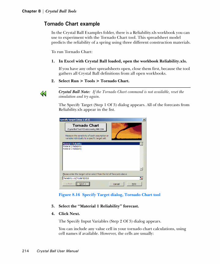
Chapter 8 | Crystal Ball Tools
Tornado Chart exampleIn the Crystal Ball Examples folder, there is a Reliability.xls workbook you can use to experiment with the Tornado Chart tool. This spreadsheet model predicts the reliability of a spring using three different construction materials.
To run Tornado Chart:
1. In Excel with Crystal Ball loaded, open the workbook Reliability.xls.
If you have any other spreadsheets open, close them first, because the tool gathers all Crystal Ball definitions from all open workbooks.
2. Select Run > Tools > Tornado Chart.
Crystal Ball Note: If the Tornado Chart command is not available, reset the simulation and try again.
The Specify Target (Step 1 Of 3) dialog appears. All of the forecasts from Reliability.xls appear in the list.
Figure 8.16 Specify Target dialog, Tornado Chart tool
3. Select the “Material 1 Reliability” forecast.
4. Click Next.
The Specify Input Variables (Step 2 Of 3) dialog appears.
You can include any value cell in your tornado chart calculations, using cell names if available. However, the cells are usually:
214 Crystal Ball User Manual

Tornado Chart tool1
Crystal Ball Note: Precedents for this tool are handled differently than standard Excel precedents in that they cannot trace beyond the active worksheet. Therefore, you can only use precedents on the active worksheet as input variables.
5. Click Add Assumptions.
Available assumptions appear in the dialog, as shown in Figure 8.17.
Figure 8.17 Specify Input Variables dialog, Tornado Chart tool
6. Remove Material 2 Strength and Material 3 Strength.
a. Select an assumption to remove.
b. Click Remove.
c. Repeat steps 6a and 6b for the second assumption to remove.
Table 8.4 Tornado chart input cells
assumptions Cells defined as assumptions in Crystal Ball. For more information about assumptions, see “Defining assumptions” on page 18.
decision variables Cells defined as decision variables in Crystal Ball. For more information about defining decision variables, see “Defining decision variable cells” on page 58.
precedents All cells within the active worksheet that are referenced as part of the formula or a sub-formula of the target cell.
Crystal Ball User Manual 215
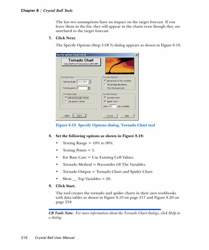
Chapter 8 | Crystal Ball Tools
The last two assumptions have no impact on the target forecast. If you leave them in the list, they will appear in the charts even though they are unrelated to the target forecast.
7. Click Next.
The Specify Options (Step 3 Of 3) dialog appears as shown in Figure 8.18.
Figure 8.18 Specify Options dialog, Tornado Chart tool
8. Set the following options as shown in Figure 8.18:
• Testing Range = 10% to 90%.
• Testing Points = 5.
• For Base Case = Use Existing Cell Values.
• Tornado Method = Percentiles Of The Variables.
• Tornado Output = Tornado Chart and Spider Chart.
• Show __ Top Variables = 20.
9. Click Start.
The tool creates the tornado and spider charts in their own workbooks with data tables as shown in Figure 8.19 on page 217 and Figure 8.20 on page 218.
CB Tools Note: For more information about the Tornado Chart dialogs, click Help in a dialog.
216 Crystal Ball User Manual

Tornado Chart tool1
Interpreting the results
In this example, six assumptions are listed in the tornado chart. The first assumption, Material 1 Strength, has the highest sensitivity ranking and is the most important. A researcher running this model would investigate this assumption further in the hopes of reducing its uncertainty and, therefore, its effect on the target forecast, Material 1 Reliability.
The last two assumptions, Wire Diameter and Spring Deflection, are the least influential assumptions. Since their effects on the Material 1 Reliability are very small, you might ignore their uncertainty or eliminate them from the spreadsheet.
Figure 8.19 Tornado chart with data
The spider chart shows similar information. Material 1, at the top of the tornado chart, has the steepest positive slope in the spider chart. Notice that more reliability values are given, one for each of five levels within the testing range.
Crystal Ball User Manual 217

Chapter 8 | Crystal Ball Tools
Figure 8.20 Spider chart with data
LimitationsWhile tornado and spider charts are very useful, there are some limitations:
• Since the tool tests each variable independently of the others, the tool doesn’t consider correlations defined between the variables.
• The results shown in the tornado and spider charts depend significantly on the particular base case used for the variables. To confirm the accuracy of the results, run the tool multiple times with different base cases.
This characteristic makes the one-at-a-time perturbation method less robust than the correlation-based method built into Crystal Ball's sensitivity chart. Hence, the sensitivity chart is preferable, since it computes sensitivity by sampling the variables all together while a simulation is running.
218 Crystal Ball User Manual

Bootstrap tool1
Bootstrap toolBootstrap is a simple technique that estimates the reliability or accuracy of forecast statistics or other sample data. Classical methods rely on mathematical formulas to describe the accuracy of sample statistics. These methods assume that the distribution of a sample statistic approaches a normal distribution, making the calculation of the statistic’s standard error or confidence interval relatively easy. However, when a statistic’s sampling distribution is not normally distributed or easily found, these classical methods are difficult to use or are invalid.
Figure 8.21 Sampling distribution of a mean statistic
In contrast, bootstrapping analyzes sample statistics empirically by repeatedly sampling the data and creating distributions of the different statistics from each sampling. The term bootstrap comes from the saying, “to pull oneself up by one’s own bootstraps,” since this method uses the distribution of statistics itself to analyze the statistics’ accuracy.
There are two bootstrap methods available with this tool:
Table 8.5 Supported bootstrap methods
One-simulation method
Simulates the model data once (creating the original sample) and then repeatedly resamples those simulation trials (the original sample values). Resampling creates a new sample from the original sample with replacement. That is, it returns the selected value to the sample before selecting another value, letting the selector possibly reselect the same value. It then creates a distribution of the statistics calculated from each resample.This method assumes only that the original simulation data accurately portrays the true forecast distribution, which is likely if the sample is large enough. This method isn’t as accurate as the multiple-simulation method, but it takes significantly less time to run.
Crystal Ball User Manual 219
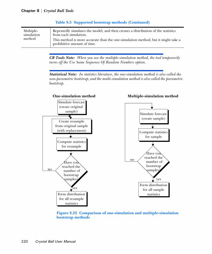
Chapter 8 | Crystal Ball Tools
CB Tools Note: When you use the multiple-simulation method, the tool temporarily turns off the Use Same Sequence Of Random Numbers option.
Statistical Note: In statistics literature, the one-simulation method is also called the non-parametric bootstrap, and the multi-simulation method is also called the parametric bootstrap.
Figure 8.22 Comparison of one-simulation and multiple-simulation bootstrap methods
Multiple-simulation method
Repeatedly simulates the model, and then creates a distribution of the statistics from each simulation.This method is more accurate than the one-simulation method, but it might take a prohibitive amount of time.
Table 8.5 Supported bootstrap methods (Continued)
Simulate forecast(create original
Create resamplefrom original sample
sample)
(with replacement)
Compute statisticsfor resample
Form distributionfor all resample
statistics
One-simulation method
Simulate forecast(create sample)
Compute statisticsfor sample
Have you
number ofbootstrap
Form distributionfor all sample
statistics
reached the
Multiple-simulation method
yes
no
yes
no samples?
Have you
number ofbootstrap
reached the
samples?
220 Crystal Ball User Manual
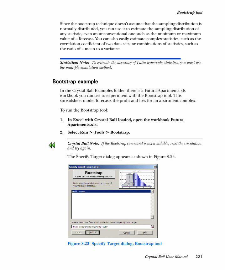
Bootstrap tool1
Since the bootstrap technique doesn’t assume that the sampling distribution is normally distributed, you can use it to estimate the sampling distribution of any statistic, even an unconventional one such as the minimum or maximum value of a forecast. You can also easily estimate complex statistics, such as the correlation coefficient of two data sets, or combinations of statistics, such as the ratio of a mean to a variance.
Statistical Note: To estimate the accuracy of Latin hypercube statistics, you must use the multiple-simulation method.
Bootstrap exampleIn the Crystal Ball Examples folder, there is a Futura Apartments.xls workbook you can use to experiment with the Bootstrap tool. This spreadsheet model forecasts the profit and loss for an apartment complex.
To run the Bootstrap tool:
1. In Excel with Crystal Ball loaded, open the workbook Futura Apartments.xls.
2. Select Run > Tools > Bootstrap.
Crystal Ball Note: If the Bootstrap command is not available, reset the simulation and try again.
The Specify Target dialog appears as shown in Figure 8.23.
Figure 8.23 Specify Target dialog, Bootstrap tool
Crystal Ball User Manual 221
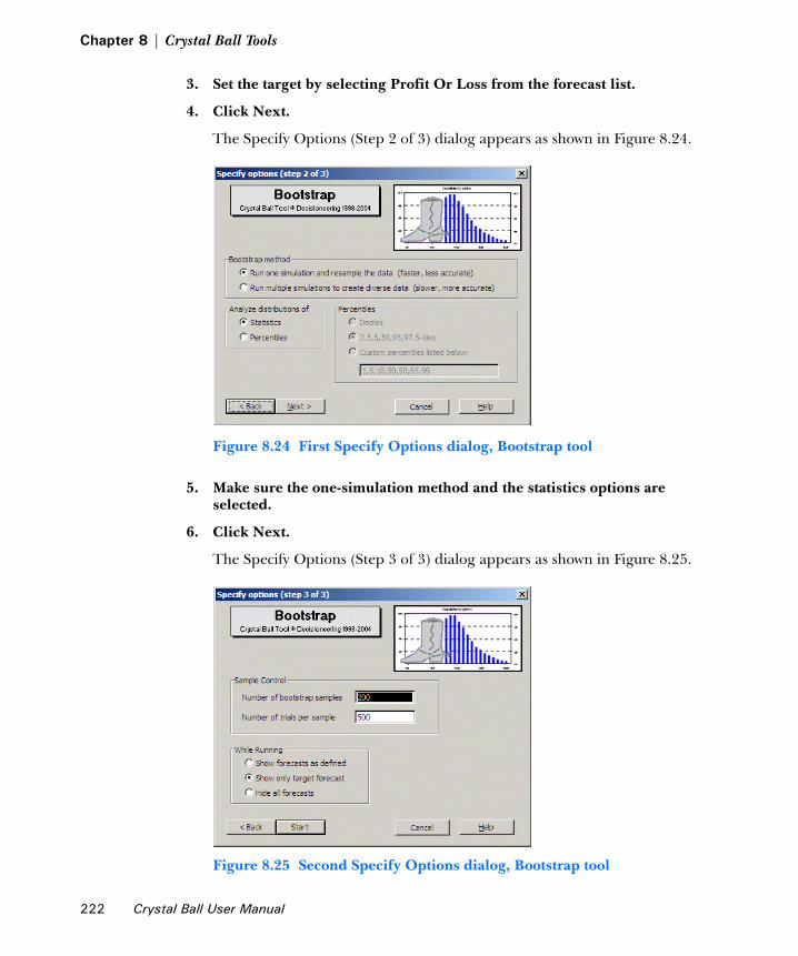
Chapter 8 | Crystal Ball Tools
3. Set the target by selecting Profit Or Loss from the forecast list.
4. Click Next.
The Specify Options (Step 2 of 3) dialog appears as shown in Figure 8.24.
Figure 8.24 First Specify Options dialog, Bootstrap tool
5. Make sure the one-simulation method and the statistics options are selected.
6. Click Next.
The Specify Options (Step 3 of 3) dialog appears as shown in Figure 8.25.
Figure 8.25 Second Specify Options dialog, Bootstrap tool
222 Crystal Ball User Manual

Bootstrap tool1
7. Set the following options:
• Number Of Bootstrap = 200
• Number Of Trials Per Sample = 500
• Show Only Target Forecast is selected
8. Click Start.
The bootstrap tool displays a forecast chart of the distributions for each statistic and creates a workbook summarizing the data.
Figure 8.26 Bootstrap example results
CB Tools Note: For more information about the Bootstrap dialogs, click Help in a dialog.
Crystal Ball User Manual 223

Chapter 8 | Crystal Ball Tools
Interpreting the results
The Bootstrap tool displays sampling distributions in forecast charts for the following statistics:
• Mean
• Median
• Standard deviation
• Variance
• Skewness
• Kurtosis
• Coefficient of variability (one simulation)
When you use the multiple-simulation method, the tool also displays sampling distributions for these statistics:
• Range minimum
• Range maximum
• Range width
For percentiles, the Bootstrap tool displays the percentile sampling distributions on the overlay and trend charts. To display the individual percentile forecast charts, select Analyze > Forecast Charts.
Crystal Ball Note: If you have the Probability Above A Value option selected in the Run Preferences > Options dialog, the percentiles are reversed in meaning, so that the 1st percentile represents the uppermost 1% and the 99th percentile represents the lowest 1%. For more information on this reversal, See “Statistics preferences” on page 87.
The forecast charts visually indicate the accuracy of each statistic. A narrow and symmetrical distribution yields more precise statistics estimates than a wide and skewed distribution.
224 Crystal Ball User Manual

Bootstrap tool1
Figure 8.27 Bootstrap forecast chart of mean
The Statistics view further lets you analyze the statistics’ sampling distribution. If the mean standard error or coefficient of variability is very large, the statistic might not be reliable and might require more samples or more trials. This example has a relatively low standard error and coefficient of variability, so the forecast mean is an accurate estimate of the population mean.
Figure 8.28 Bootstrap forecast statistics for the mean
Crystal Ball User Manual 225

Chapter 8 | Crystal Ball Tools
The results workbook has a correlation matrix showing the correlations between the various statistics. High correlation between certain statistics, such as between the mean and the standard deviation, usually indicates a highly skewed distribution.
You can also use the Bootstrap tool to analyze the distribution of percentiles, but you should run at least 1,000 bootstrap samples and 1,000 trials per sample to obtain good sampling distributions for these statistics (according to Efron and Tibshirani; see Bibliography).
Decision Table toolDecision variables are values that you can control, such as how much to charge for a product or how many wells to drill. But, in situations with uncertainty, it is not always obvious what effect changing a decision variable can have on the forecast results.
The Decision Table tool runs multiple simulations to test different values for one or two decision variables. The tool tests values across the range of the decision variables and puts the results in a table that you can analyze using Crystal Ball forecast, trend, or overlay charts.
The Decision Table tool is useful for investigating how changes in the values of a few decision variable affect the forecast results. For models that contain more than a handful of decision variables, or where you are trying to optimize the forecast results, use OptQuest for Crystal Ball.
OptQuest is a wizard-based program that enhances Crystal Ball by automatically finding optimal solutions to simulation models. This program is available with Crystal Ball Professional and Premium Editions.
226 Crystal Ball User Manual
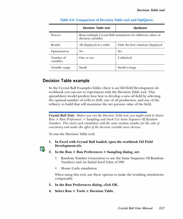
Decision Table tool1
Decision Table exampleIn the Crystal Ball Examples folder, there is an Oil Field Development.xls workbook you can use to experiment with the Decision Table tool. This spreadsheet model predicts how best to develop a new oil field by selecting the optimal number of wells to drill, rate of oil production, and size of the refinery to build that will maximize the net present value of the field.
Crystal Ball Note: Before you run the Decision Table tool, you might want to choose Run > Run Preferences > Sampling and check Use Same Sequence Of Random Numbers. This starts each simulation with the same random number for the sake of consistency and makes the effect of the decision variable more obvious.
To run the Decision Table tool:
1. In Excel with Crystal Ball loaded, open the workbook Oil Field Development.xls.
2. In the Run > Run Preferences > Sampling dialog, set:
• Random Number Generation to use the Same Sequence Of Random Numbers and An Initial Seed Value of 999
• Monte Carlo simulation
When using this tool, use these options to make the resulting simulations comparable.
3. In the Run Preferences dialog, click OK.
4. Select Run > Tools > Decision Table.
Table 8.6 Comparison of Decision Table tool and OptQuest.
Decision Table tool OptQuest
Process Runs multiple Crystal Ball simulations for different values of decision variables
Results All displayed in a table Only the best solutions displayed
Optimization No Yes
Number of variables
One or two Unlimited
Variable range Small Small to large
Crystal Ball User Manual 227
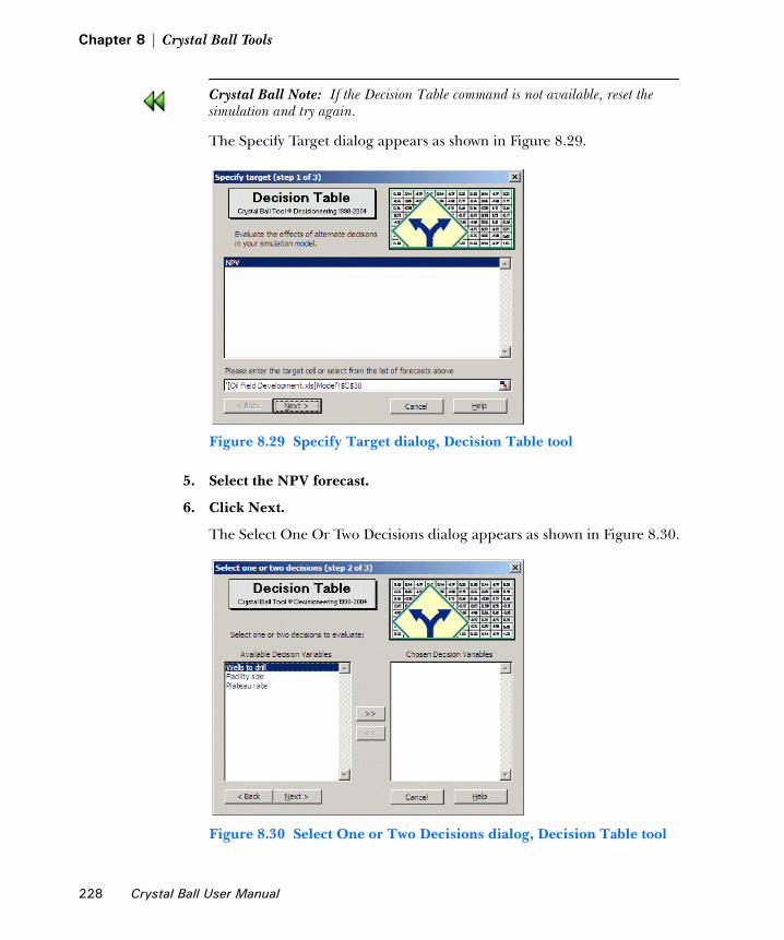
Chapter 8 | Crystal Ball Tools
Crystal Ball Note: If the Decision Table command is not available, reset the simulation and try again.
The Specify Target dialog appears as shown in Figure 8.29.
Figure 8.29 Specify Target dialog, Decision Table tool
5. Select the NPV forecast.
6. Click Next.
The Select One Or Two Decisions dialog appears as shown in Figure 8.30.
Figure 8.30 Select One or Two Decisions dialog, Decision Table tool
228 Crystal Ball User Manual

Decision Table tool1
7. Move Wells To Drill and Facility Size to the Chosen Decision Variables list.
a. Select Wells To Drill in the Available Decision Variables field.
b. Click >>.
c. Repeat steps 7a and 7b for the Facility Size.
8. Click Next.
The Specify Options dialog appears as shown in Figure 8.31.
Figure 8.31 Specify Options dialog, Decision Table tool
9. Set the following options as shown above:
• Number of values to test for Wells To Drill = 6.
• Number of values to test for Facility Size = 7.
• Maximum trials per simulation = 500.
• Show Only Target Forecast is selected.
10. Click Start.
The tool runs a simulation for each combination of decision variable values. It compiles the results in a table of forecast cells indexed by the decision variables.
CB Tools Note: For more information on the Decision Table dialogs, click Help in a dialog.
Crystal Ball User Manual 229

Chapter 8 | Crystal Ball Tools
Interpreting the results
For this example, the Decision Table tool ran 42 simulations, one for each combination of wells to drill and facility sizes. The simulation that resulted in the best mean NPV was the combination of 12 wells and a facility size of 150 mbd.
Figure 8.32 Decision table for Oil Field Development results
To view one or more of the forecasts in the decision table, select the cells and click Forecast Charts. To compare one or more forecasts on the same chart, select the cells and click Trend Chart or Overlay Chart.
Figure 8.33 Trend chart of 150 mbd forecasts
230 Crystal Ball User Manual
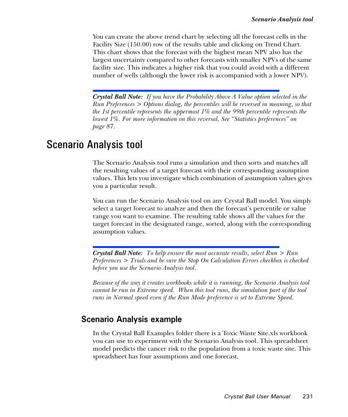
Scenario Analysis tool1
You can create the above trend chart by selecting all the forecast cells in the Facility Size (150.00) row of the results table and clicking on Trend Chart. This chart shows that the forecast with the highest mean NPV also has the largest uncertainty compared to other forecasts with smaller NPVs of the same facility size. This indicates a higher risk that you could avoid with a different number of wells (although the lower risk is accompanied with a lower NPV).
Crystal Ball Note: If you have the Probability Above A Value option selected in the Run Preferences > Options dialog, the percentiles will be reversed in meaning, so that the 1st percentile represents the uppermost 1% and the 99th percentile represents the lowest 1%. For more information on this reversal, See “Statistics preferences” on page 87.
Scenario Analysis toolThe Scenario Analysis tool runs a simulation and then sorts and matches all the resulting values of a target forecast with their corresponding assumption values. This lets you investigate which combination of assumption values gives you a particular result.
You can run the Scenario Analysis tool on any Crystal Ball model. You simply select a target forecast to analyze and then the forecast’s percentile or value range you want to examine. The resulting table shows all the values for the target forecast in the designated range, sorted, along with the corresponding assumption values.
Crystal Ball Note: To help ensure the most accurate results, select Run > Run Preferences > Trials and be sure the Stop On Calculation Errors checkbox is checked before you use the Scenario Analysis tool. Because of the way it creates workbooks while it is running, the Scenario Analysis tool cannot be run in Extreme speed. When this tool runs, the simulation part of the tool runs in Normal speed even if the Run Mode preference is set to Extreme Speed.
Scenario Analysis exampleIn the Crystal Ball Examples folder there is a Toxic Waste Site.xls workbook you can use to experiment with the Scenario Analysis tool. This spreadsheet model predicts the cancer risk to the population from a toxic waste site. This spreadsheet has four assumptions and one forecast.
Crystal Ball User Manual 231

Chapter 8 | Crystal Ball Tools
Figure 8.34 Toxic Waste Site spreadsheet
To run the Scenario Analysis tool:
1. In Excel with Crystal Ball loaded, open the workbook Toxic Waste Site.xls.
2. Select Run > Tools > Scenario Analysis.
Crystal Ball Note: If the Scenario Analysis command is not available, reset the simulation and try again.
The Specify Target dialog appears as shown in Figure 8.35.
Figure 8.35 Specify Target dialog, Scenario Analysis tool
232 Crystal Ball User Manual

Scenario Analysis tool1
3. Select the Risk Assessment forecast.
4. Click Next.
The Specify Options dialog appears.
Figure 8.36 Specify Options dialog, Scenario Analysis tool
5. In the Range Of Forecast Results section, specify a percentile range from 95 to 100 percent.
6. In the While Running section, select Show Only Target Forecast.
7. In the Simulation Control section, enter 1000 as the maximum number of trials to run.
8. Click Start.
The tool creates a table of all the forecast values within the range specified in step 5, along with the corresponding value of each assumption as shown in Figure 8.37.
Crystal Ball User Manual 233

Chapter 8 | Crystal Ball Tools
Figure 8.37 Scenario Analysis results for Toxic Waste Site
Windows Note: For the next few steps, you might want to arrange the windows in Excel vertically, so that you can see the results next to the original workbook.
9. Select the row with the 98.00% (assuming default percentile settings).
10. Click Paste Selected Scenario.
The scenario of assumption values that produced the 98th percentile value of the target forecast appears in the Toxic Waste workbook. Crystal Ball recalculates the workbook and updates the forecast cells.
11. Click Paste Next Scenario.
In the workbook, the assumption and forecast values change to the values for the next scenario (for 98.10%).
12. Click Reset Original Values.
The original assumption and forecast values appear in the workbook.
CB Tools Note: For more information about the Scenario Analysis dialogs, click Help in a dialog.
234 Crystal Ball User Manual

Scenario Analysis tool1
Interpreting the results
In this example, the simulation generated 1,000 forecast values. Since you selected to analyze the percentiles from 95 to 100, the resulting table lists 51 forecast values, or the top 5% of the forecast range, including the endpoints. The table sorts the values from lowest to highest value and also includes the assumption values that Crystal Ball generated for each trial.
Crystal Ball Note: If you have the Probability Above A Value option selected in the Run Preferences > Options dialog, the percentiles will be reversed in meaning, so that the 1st percentile represents the uppermost 1% and the 99th percentile represents the lowest 1%.
One way to analyze the Scenario Analysis results is to identify a particular forecast value and see what assumption values created that forecast value.
Another way to analyze the Scenario Analysis results is to generate an Excel chart with the data. For example, you might create a scatter chart comparing the risk assessment with the CPF, as shown below.
Figure 8.38 Scatter chart of Risk Assessment and CPF
Crystal Ball User Manual 235

Chapter 8 | Crystal Ball Tools
Two-Dimensional Simulation toolRisk analysts must often consider two sources of variation in their models:
For many types of risk assessments, it is important to clearly distinguish between uncertainty and variability (see Hoffman and Hammonds reference, page 361). Separating these concepts in a simulation lets you more accurately detect the variation in a forecast due to lack of knowledge and the variation caused by natural variability in a measurement or population. In the same way that a one-dimensional simulation is generally better than single-point estimates for showing the true probability of risk, a two-dimensional simulation is generally better than a one-dimensional simulation for characterizing risk.
The Two-Dimensional Simulation tool runs an outer loop to simulate the uncertainty values, and then freezes the uncertainty values while it runs an inner loop (of the whole model) to simulate the variability. This process repeats for some number of outer simulations, providing a portrait of how the forecast distribution varies due to the uncertainty.
The primary output of this process is a chart depicting a series of cumulative frequency distributions. You can interpret this chart as the range of possible risk curves associated with a population.
CB Tools Note: When using this tool, set the Seed Value option in the Crystal Ball Run Preferences dialog so that the resulting simulations are more comparable.
Table 8.7 Sources of model variation
uncertainty Assumptions that are uncertain because you have insufficient information about a true, but unknown, value. Examples of uncertainty include the reserve size of an oil field and the prime interest rate in 12 months. You can describe an uncertainty assumption with a probability distribution.Theoretically, you can eliminate uncertainty by gathering more information. Practically, information can be missing because you haven’t gathered it or because it is too costly to gather.
variability Assumptions that change because they describe a population with different values. Examples of variability include the individual body weights in a population or the daily number of products sold over a year. You can describe a variability assumption with a discrete distribution (or approximate one with a continuous distribution).Variability is inherent in the system, and you cannot eliminate it by gathering more information.
236 Crystal Ball User Manual
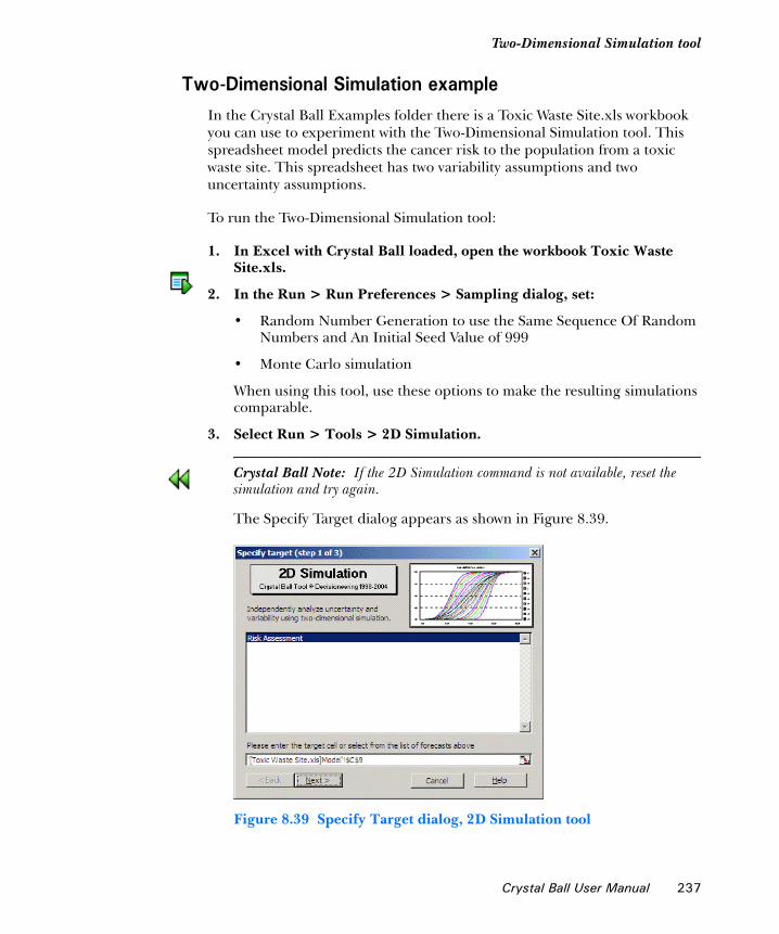
Two-Dimensional Simulation tool1
Two-Dimensional Simulation exampleIn the Crystal Ball Examples folder there is a Toxic Waste Site.xls workbook you can use to experiment with the Two-Dimensional Simulation tool. This spreadsheet model predicts the cancer risk to the population from a toxic waste site. This spreadsheet has two variability assumptions and two uncertainty assumptions.
To run the Two-Dimensional Simulation tool:
1. In Excel with Crystal Ball loaded, open the workbook Toxic Waste Site.xls.
2. In the Run > Run Preferences > Sampling dialog, set:
• Random Number Generation to use the Same Sequence Of Random Numbers and An Initial Seed Value of 999
• Monte Carlo simulation
When using this tool, use these options to make the resulting simulations comparable.
3. Select Run > Tools > 2D Simulation.
Crystal Ball Note: If the 2D Simulation command is not available, reset the simulation and try again.
The Specify Target dialog appears as shown in Figure 8.39.
Figure 8.39 Specify Target dialog, 2D Simulation tool
Crystal Ball User Manual 237

Chapter 8 | Crystal Ball Tools
4. Select the Risk Assessment forecast.
5. Click Next.
The Specify Assumptions dialog appears as shown in Figure 8.40.
Figure 8.40 Specify Assumptions dialog, 2D Simulation tool
6. Move Body Weight and Volume Of Water Per Day to the Variability list.
a. Select Body Weight.
b. Click >>.
c. Repeat steps 6a and 6b for Volume Of Water Per Day.
This separates the assumptions into the two types: uncertainty and variability.
7. Click Next.
The Specify Options dialog appears as shown in Figure 8.41.
238 Crystal Ball User Manual

Two-Dimensional Simulation tool1
Figure 8.41 Specify Options dialog, 2D Simulation tool
8. Set the following options.
• Number of trials for the outer simulation = 100
• Maximum trials for the inner simulation = 1,000
• Show Only Target Forecast is selected.
9. Click Start.
The simulations start. The tool first single-steps one trial to generate a new set of values for the uncertainty assumptions. Then it freezes these assumptions and runs a simulation for the variability assumptions in the inner loop.
The tool retrieves the Crystal Ball forecast information after each inner loop runs. The tool then resets the simulation and repeats the process until the outer loop has run for the specified number of simulations.
CB Tools Note: For more information on the 2D Simulation tool dialogs, click Help in a dialog.
Interpreting the results
The results of the simulations appear in a table containing the forecast means, the uncertainty assumption values, and the statistics (including percentiles) of the forecast distribution for each simulation.
Crystal Ball User Manual 239

Chapter 8 | Crystal Ball Tools
Figure 8.42 Two-Dimensional Simulation results table
The tool also graphs the results of the two-dimensional simulations on an overlay chart and a trend chart.
The overlay chart preferences can be set to show the risk curves for the simulations for different sets of uncertainty assumption values. To do this, set the Chart Type for each series to Line and choose Cumulative Frequency view. It is convenient to use the chart hotkeys — Ctrl-t for the chart type and Ctrl-d for view. Optionally, use Ctrl-n to move or remove the legend and Ctrl-m to cycle through central tendency marker lines.
For this example, Figure 8.43 shows that most of the risk curves are clustered densely toward the center while a few outlier curves are scattered to the right, showing the small probability of having a much greater risk.
Statistical Note: In risk analysis literature, the curves are often called the alternate realizations of the population risk assessment.
240 Crystal Ball User Manual

Two-Dimensional Simulation tool1
Figure 8.43 Overlay chart of risk curves
The trend chart shows certainty bands for the percentiles of the risk curves. The band width shows the amount of uncertainty at each percentile level for all the distributions.
Figure 8.44 Trend chart of certainty bands
Crystal Ball User Manual 241
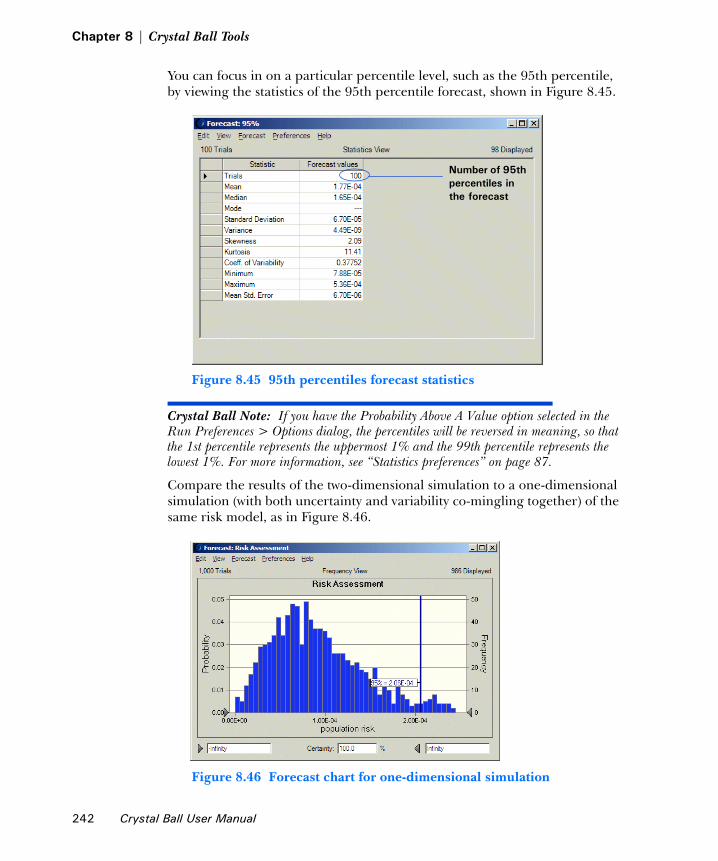
Chapter 8 | Crystal Ball Tools
You can focus in on a particular percentile level, such as the 95th percentile, by viewing the statistics of the 95th percentile forecast, shown in Figure 8.45.
Figure 8.45 95th percentiles forecast statistics
Crystal Ball Note: If you have the Probability Above A Value option selected in the Run Preferences > Options dialog, the percentiles will be reversed in meaning, so that the 1st percentile represents the uppermost 1% and the 99th percentile represents the lowest 1%. For more information, see “Statistics preferences” on page 87.
Compare the results of the two-dimensional simulation to a one-dimensional simulation (with both uncertainty and variability co-mingling together) of the same risk model, as in Figure 8.46.
Figure 8.46 Forecast chart for one-dimensional simulation
Number of 95th percentiles in the forecast
242 Crystal Ball User Manual

Two-Dimensional Simulation tool1
The mean of the 95th percentiles, 1.77E-4, is lower than the 95th percentile risk of the one-dimensional simulation shown above at 2.06E-4. This indicates the tendency of the one-dimensional simulation results to overestimate the population risk, especially for highly skewed distributions.
Second-order assumptionsSome assumptions contain elements of both uncertainty and variability. For instance, an assumption might describe the distribution of body weights in a population, but the parameters of the distribution might be uncertain. These types of assumptions are called second-order assumptions (also, second-order random variables; see Burmaster and Wilson, 1996, in the Bibliography). You can model these types of assumptions in Crystal Ball by placing the uncertain parameters of the distribution in separate cells and defining these cells as assumptions. You then link the parameters of the variability assumption to the uncertainty assumptions using cell references.
To illustrate this for the Toxic Waste Site.xls spreadsheet:
1. Enter the values 70 and 10 into cells G4 and G5, respectively.
These are the mean and standard deviation of the Body Weight assumption in cell C4, which is defined as a normal distribution.
2. Define an assumption for cell G4 using a normal distribution with a mean of 70 and a standard deviation of 2.
3. Define an assumption for cell G5 using a normal distribution with a mean of 10 and a standard deviation of 1.
4. Enter references to these cells in the Body Weight assumption.
For an example, see Figure 8.47, following.
Crystal Ball User Manual 243

Chapter 8 | Crystal Ball Tools
Figure 8.47 Assumption using cell references for the mean and standard deviation
When you run the tool for second-order assumptions, the uncertainty of the assumptions’ parameters is modeled in the outer simulation, and the distribution of the assumption itself is modeled (for different sets of parameters) in the inner simulation.
Crystal Ball Note: Often, the parameters of assumptions are correlated. For example, you would correlate a higher mean with a higher standard deviation or a lower mean with a lower standard deviation. Defining correlation coefficients between parameter distributions can increase the accuracy of your two-dimensional simulation. With data available, as in sample body weights of a population, you can use the Bootstrap tool to estimate the sampling distributions of the parameters and the correlations between them.
244 Crystal Ball User Manual

Appendix ASelecting and Using Probability Distributions
In this appendix• Understanding probability
distributions
• Selecting a probability distribution
• Using basic distributions
• Using continuous distributions
• Using discrete distributions
• Using the custom distribution
• Truncating distributions
• Comparing the distributions
This appendix explains probability and probability distributions. Understanding these concepts will help you select the right probability distribution for your spreadsheet model. This section describes in detail the distribution types Crystal Ball uses and demonstrates their use with real-world examples.
Crystal Ball User Manual 245

Appendix A | Selecting and Using Probability Distributions
Understanding probability distributionsFor each uncertain variable in a simulation, you define the possible values with a probability distribution. The type of distribution you select depends on the conditions surrounding the variable. For example, some common distribution types are:
Figure A.1 Common distribution types
During a simulation, the value to use for each variable is selected randomly from the defined possibilities.
A simulation calculates numerous scenarios of a model by repeatedly picking values from the probability distribution for the uncertain variables and using those values for the cell. Commonly, a Crystal Ball simulation calculates hundreds or thousands of scenarios in just a few seconds.
A probability exampleTo begin to understand probability, consider this example: You want to look at the distribution of non-exempt wages within one department of a large company. First, you gather raw data, in this case the wages of each non-exempt employee in the department. Second, you organize the data into a meaningful format and plot the data as a frequency distribution on a chart. To create a frequency distribution, you divide the wages into groups (also called intervals or bins) and list these intervals on the chart’s horizontal axis. Then you list the number or frequency of employees in each interval on the chart’s vertical axis. Now you can easily see the distribution of non-exempt wages within the department.
A glance at the chart illustrated in Figure A.2 reveals that the most common wage range is $12.00 to $15.00.
Approximately 60 employees (out of a total of 180) earn from $12 to $15.00 per hour.
246 Crystal Ball User Manual
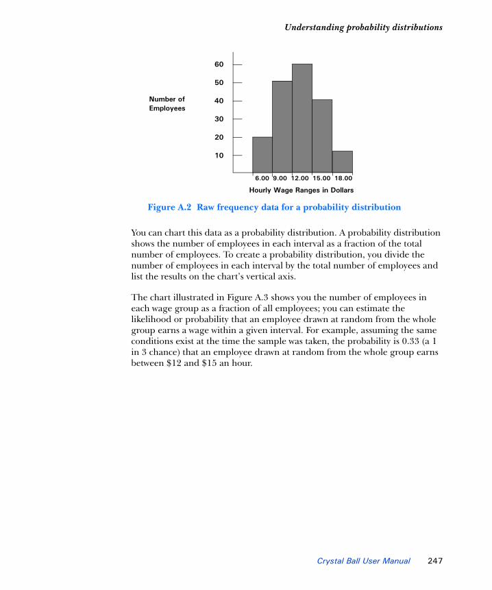
Understanding probability distributions1
Figure A.2 Raw frequency data for a probability distribution
You can chart this data as a probability distribution. A probability distribution shows the number of employees in each interval as a fraction of the total number of employees. To create a probability distribution, you divide the number of employees in each interval by the total number of employees and list the results on the chart’s vertical axis.
The chart illustrated in Figure A.3 shows you the number of employees in each wage group as a fraction of all employees; you can estimate the likelihood or probability that an employee drawn at random from the whole group earns a wage within a given interval. For example, assuming the same conditions exist at the time the sample was taken, the probability is 0.33 (a 1 in 3 chance) that an employee drawn at random from the whole group earns between $12 and $15 an hour.
Number of Employees
60
50
40
30
20
10
Hourly Wage Ranges in Dollars
6.00 9.00 12.00 15.00 18.00
Crystal Ball User Manual 247

Appendix A | Selecting and Using Probability Distributions
Figure A.3 Probability distribution of wages
Compare the probability distribution in the example above to the probability distributions in Crystal Ball (Figure A.4).
Figure A.4 Distribution Gallery dialog
Probability
0.33 0.22 0.11
Hourly Wage Ranges in Dollars
6.00 9.00 12.00 15.00 18.00
248 Crystal Ball User Manual
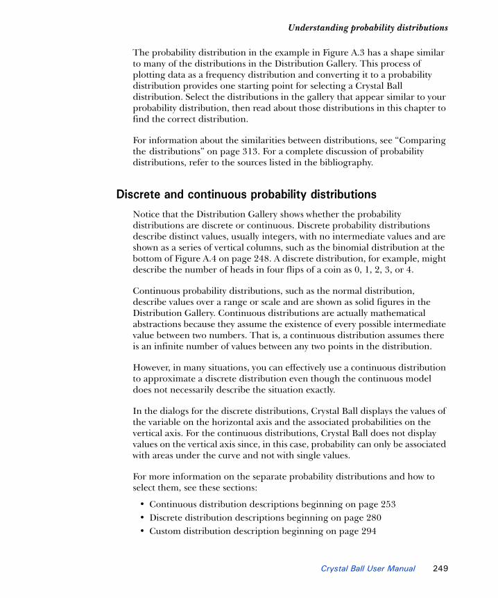
Understanding probability distributions1
The probability distribution in the example in Figure A.3 has a shape similar to many of the distributions in the Distribution Gallery. This process of plotting data as a frequency distribution and converting it to a probability distribution provides one starting point for selecting a Crystal Ball distribution. Select the distributions in the gallery that appear similar to your probability distribution, then read about those distributions in this chapter to find the correct distribution.
For information about the similarities between distributions, see “Comparing the distributions” on page 313. For a complete discussion of probability distributions, refer to the sources listed in the bibliography.
Discrete and continuous probability distributionsNotice that the Distribution Gallery shows whether the probability distributions are discrete or continuous. Discrete probability distributions describe distinct values, usually integers, with no intermediate values and are shown as a series of vertical columns, such as the binomial distribution at the bottom of Figure A.4 on page 248. A discrete distribution, for example, might describe the number of heads in four flips of a coin as 0, 1, 2, 3, or 4.
Continuous probability distributions, such as the normal distribution, describe values over a range or scale and are shown as solid figures in the Distribution Gallery. Continuous distributions are actually mathematical abstractions because they assume the existence of every possible intermediate value between two numbers. That is, a continuous distribution assumes there is an infinite number of values between any two points in the distribution.
However, in many situations, you can effectively use a continuous distribution to approximate a discrete distribution even though the continuous model does not necessarily describe the situation exactly.
In the dialogs for the discrete distributions, Crystal Ball displays the values of the variable on the horizontal axis and the associated probabilities on the vertical axis. For the continuous distributions, Crystal Ball does not display values on the vertical axis since, in this case, probability can only be associated with areas under the curve and not with single values.
For more information on the separate probability distributions and how to select them, see these sections:
• Continuous distribution descriptions beginning on page 253• Discrete distribution descriptions beginning on page 280• Custom distribution description beginning on page 294
Crystal Ball User Manual 249

Appendix A | Selecting and Using Probability Distributions
Crystal Ball Note: Initially, the precision and format of the displayed numbers in the probability and frequency distributions come from the cell itself. To change the format, see “Customizing chart axes and axis labels” on page 138.
Selecting a probability distributionPlotting data is one guide to selecting a probability distribution. The following steps provide another process for selecting probability distributions that best describe the uncertain variables in your spreadsheets.
To select the correct probability distribution:
• Look at the variable in question. List everything you know about the conditions surrounding this variable.
You might be able to gather valuable information about the uncertain variable from historical data. If historical data are not available, use your own judgment, based on experience, to list everything you know about the uncertain variable.
For example, look at the variable “patients cured” that was discussed in the Vision Research tutorial in Chapter 2 of the Crystal Ball Getting Started Guide. The company must test 100 patients. You know that the patients will either be cured or not cured. And, you know that the drug has shown a cure rate of around 0.25 (25%). These facts are the conditions surrounding the variable.
• Review the descriptions of the probability distributions.
This chapter describes each distribution in detail, outlining the conditions underlying the distribution and providing real-world examples of each distribution type. As you review the descriptions, look for a distribution that features the conditions you have listed for this variable.
• Select the distribution that characterizes this variable.
A distribution characterizes a variable when the conditions of the distribution match those of the variable.
The conditions of the variable describe the values for the parameters of the distribution in Crystal Ball. Each distribution type has its own set of parameters, which are explained in the following descriptions.
For example, look at the conditions of the binomial distribution, as described on page 281:
• For each trial, only two outcomes are possible: success or failure.
250 Crystal Ball User Manual

Selecting a probability distribution1
• The trials are independent. What happens on the first trial does not affect the second trial, and so on.
• The probability of success remains the same from trial to trial.
Now check the “patients cured” variable in Tutorial 2 in the Crystal Ball Getting Started Guide against the conditions of the binomial distribution:
• There are two possible outcomes: the patient is either cured or not cured.
• The trials (100) are independent of each other. What happens to the first patient does not affect the second patient.
• The probability of curing a patient 0.25 (25%) remains the same each time a patient is tested.
Since the conditions of the variable match the conditions of the binomial distribution, the binomial distribution would be the correct distribution type for the variable in question.
• If historical data are available, use distribution fitting to select the distribution that best describes your data.
Crystal Ball can automatically select the probability distribution that most closely approximates your data’s distribution. The feature is described in detail in “Fitting distributions to data” beginning on page 27. You can also populate a custom distribution with your historical data.
After you select a distribution type, determine the parameter values for the distribution. Each distribution type has its own set of parameters. For example, there are two parameters for the binomial distribution: trials and probability. The conditions of a variable contain the values for the parameters. In the example used, the conditions show 100 trials and 0.25 (25%) probability of success.
In addition to the standard parameter set, each continuous distribution (except uniform) also lets you choose from alternate parameter sets, which substitute percentiles for one or more of the standard parameters. For more information on alternate parameters, see “Alternate parameter sets” on page 25.
Crystal Ball User Manual 251

Appendix A | Selecting and Using Probability Distributions
Using basic distributionsThis section describes distributions in the Basic category of the Distribution Gallery.
Figure A.5 Distribution Gallery, Basic category
Basic distributions are listed below in the same order they appear above. For details, see the page references below the names.
Table A.1 Summary of basic distributions
Shape Name Summary
Normal(page 268)
The normal distribution is the most important distribution in probability theory because it describes many natural phenomena, such as people’s IQs or heights. Decision-makers can use the normal distribution to describe uncertain variables such as the inflation rate or the future price of gasoline.
Triangular(page 274)
The triangular distribution describes a situation where you know the minimum, maximum, and most likely values to occur. For example, you could describe the number of cars sold per week when past sales show the minimum, maximum, and usual number of cars sold.
Uniform(page 276)
In the uniform distribution, all values between the minimum and maximum occur with equal likelihood.
252 Crystal Ball User Manual

Using continuous distributions1
Using continuous distributionsContinuous probability distributions describe values over a range or scale and are shown as solid figures in the Distribution Gallery. Continuous distributions are actually mathematical abstractions because they assume the existence of every possible intermediate value between two numbers. That is, a continuous distribution assumes there is an infinite number of values between any two points in the distribution.
In many situations, you can effectively use a continuous distribution to approximate a discrete distribution even though the continuous model does not necessarily describe the situation exactly. For a comparison of continuous and discrete distributions, see page 249.
The continuous distributions listed in Table A.2 are described later in this section in alphabetical order. Page references appear below the names.
Lognormal(page 263)
The lognormal distribution is widely used in situations where values are positively skewed, for example in financial analysis for security valuation or in real estate for property valuation.
Yes-no(page 293)
The yes-no distribution is a discrete distribution that describes a set of observations that can have only one of two values, such as yes or no, success or failure, true or false, or heads or tails.
Discrete uniform(page 283)
In the discrete uniform distribution, all integer values between the minimum and maximum are equally likely to occur. It is the discrete equivalent of the continuous uniform distribution.
Table A.1 Summary of basic distributions (Continued)
Shape Name Summary
Table A.2 Summary of continuous distributions
Shape Name Summary
Beta(page 255)
The beta distribution is a very flexible distribution commonly used to represent variability over a fixed range. It can represent uncertainty in the probability of occurrence of an event. It is also used to describe empirical data and predict the random behavior of percentages and fractions.
Exponential(page 257)
The exponential distribution is widely used to describe events recurring at random points in time or space, such as the time between failures of electronic equipment, the time between arrivals at a service booth, or repairs needed on a certain stretch of highway. It is related to the Poisson distribution, which describes the number of occurrences of an event in a given interval of time or space.
Crystal Ball User Manual 253

Appendix A | Selecting and Using Probability Distributions
Gamma(page 259)
The gamma distribution applies to a wide range of physical quantities and is related to other distributions: lognormal, exponential, Pascal, Erlang, Poisson, and chi-squared. It is used in meteorological processes to represent pollutant concentrations and precipitation quantities. The gamma distribution is also used to measure the time between the occurrence of events when the event process is not completely random. Other applications of the gamma distribution include inventory control, economics theory, and insurance risk theory.
Logistic(page 262)
The logistic distribution is commonly used to describe growth (the size of a population expressed as a function of a time variable). It can also be used to describe chemical reactions and the course of growth for a population or individual.
Lognormal (Basic)(page 263)
The lognormal distribution is widely used in situations where values are positively skewed, for example in financial analysis for security valuation or in real estate for property valuation.
Maximum extreme(page 265)
The maximum extreme distribution is commonly used to describe the largest value of a response over a period of time: for example, in flood flows, rainfall, and earthquakes. Other applications include the breaking strengths of materials, construction design, and aircraft loads and tolerances. This distribution is also known as the Gumbel distribution. and is closely related to the minimum extreme distribution, its “mirror image.”
Minimum extreme(page 267)
The minimum extreme distribution is commonly used to describe the smallest value of a response over a period of time: for example, rainfall during a drought. This distribution is closely related to the maximum extreme distribution.
Normal (Basic)(page 268)
The normal distribution is the most important distribution in probability theory because it describes many natural phenomena, such as people’s IQs or heights. Decision-makers can use the normal distribution to describe uncertain variables such as the inflation rate or the future price of gasoline.
Pareto(page 270)
The Pareto distribution is widely used for the investigation of distributions associated with such empirical phenomena as city population sizes, the occurrence of natural resources, the size of companies, personal incomes, stock price fluctuations, and error clustering in communication circuits.
Student’s t(page 272)
The Student’s t distribution is used to describe small sets of empirical data that resemble a normal curve, but with thicker tails (more outliers). For sets of data larger than 30, you can use the normal distribution instead.
Triangular (Basic)(page 274)
The triangular distribution describes a situation where you know the minimum, maximum, and most likely values to occur. For example, you could describe the number of cars sold per week when past sales show the minimum, maximum, and usual number of cars sold.
Table A.2 Summary of continuous distributions (Continued)
Shape Name Summary
254 Crystal Ball User Manual
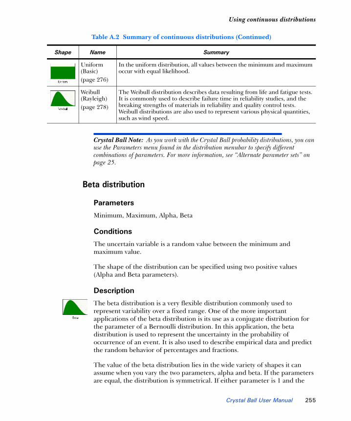
Using continuous distributions1
Crystal Ball Note: As you work with the Crystal Ball probability distributions, you can use the Parameters menu found in the distribution menubar to specify different combinations of parameters. For more information, see “Alternate parameter sets” on page 25.
Beta distribution
Parameters
Minimum, Maximum, Alpha, Beta
Conditions
The uncertain variable is a random value between the minimum and maximum value.
The shape of the distribution can be specified using two positive values (Alpha and Beta parameters).
Description
The beta distribution is a very flexible distribution commonly used to represent variability over a fixed range. One of the more important applications of the beta distribution is its use as a conjugate distribution for the parameter of a Bernoulli distribution. In this application, the beta distribution is used to represent the uncertainty in the probability of occurrence of an event. It is also used to describe empirical data and predict the random behavior of percentages and fractions.
The value of the beta distribution lies in the wide variety of shapes it can assume when you vary the two parameters, alpha and beta. If the parameters are equal, the distribution is symmetrical. If either parameter is 1 and the
Uniform (Basic)(page 276)
In the uniform distribution, all values between the minimum and maximum occur with equal likelihood.
Weibull (Rayleigh)(page 278)
The Weibull distribution describes data resulting from life and fatigue tests. It is commonly used to describe failure time in reliability studies, and the breaking strengths of materials in reliability and quality control tests. Weibull distributions are also used to represent various physical quantities, such as wind speed.
Table A.2 Summary of continuous distributions (Continued)
Shape Name Summary
Crystal Ball User Manual 255
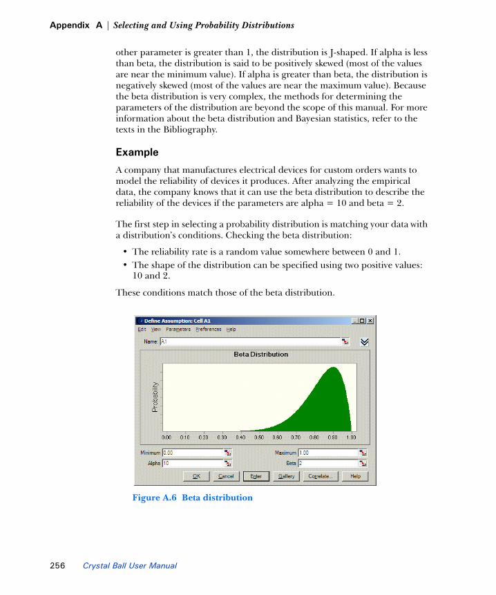
Appendix A | Selecting and Using Probability Distributions
other parameter is greater than 1, the distribution is J-shaped. If alpha is less than beta, the distribution is said to be positively skewed (most of the values are near the minimum value). If alpha is greater than beta, the distribution is negatively skewed (most of the values are near the maximum value). Because the beta distribution is very complex, the methods for determining the parameters of the distribution are beyond the scope of this manual. For more information about the beta distribution and Bayesian statistics, refer to the texts in the Bibliography.
Example
A company that manufactures electrical devices for custom orders wants to model the reliability of devices it produces. After analyzing the empirical data, the company knows that it can use the beta distribution to describe the reliability of the devices if the parameters are alpha = 10 and beta = 2.
The first step in selecting a probability distribution is matching your data with a distribution’s conditions. Checking the beta distribution:
• The reliability rate is a random value somewhere between 0 and 1.• The shape of the distribution can be specified using two positive values:
10 and 2.
These conditions match those of the beta distribution.
Figure A.6 Beta distribution
256 Crystal Ball User Manual

Using continuous distributions1
Figure A.6 shows the beta distribution with the alpha parameter set to 10, the beta parameter set to 2, and Minimum and Maximum set to 0 and 1. The reliability rate of the devices will be x.
Exponential distribution
Parameter
Rate
Conditions
The exponential distribution describes the amount of time between occurrences.
The distribution is not affected by previous events.
Description
The exponential distribution is widely used to describe events recurring at random points in time or space, such as the time between failures of electronic equipment, the time between arrivals at a service booth, or repairs needed on a certain stretch of highway. It is related to the Poisson distribution, which describes the number of occurrences of an event in a given interval of time or space.
An important characteristic of the exponential distribution is the “memoryless” property, which means that the future lifetime of a given object has the same distribution, regardless of the time it existed. In other words, time has no effect on future outcomes.
Example one
A travel agency wants to describe the time between incoming telephone calls when the calls are averaging about 35 every 10 minutes. This same example was used for the Poisson distribution to describe the number of calls arriving every 10 minutes.
The first step in selecting a probability distribution is matching your data with a distribution’s conditions. Checking the exponential distribution:
• The travel agency wants to describe the time between successive telephone calls.
• The phone calls are not affected by previous history. The probability of receiving 35 calls every 10 minutes remains the same.
Crystal Ball User Manual 257

Appendix A | Selecting and Using Probability Distributions
The conditions in this example match those of the exponential distribution.
The exponential distribution has only one parameter: rate. The conditions outlined in this example include the value for this parameter: 35 (calls) every minute or a rate of 35. Enter this value to set the parameter of the exponential distribution in Crystal Ball.
Figure A.7 Exponential distribution
The distribution in Figure A.7 shows the probability that x number of time units (10 minutes in this case) will pass between calls.
Example two
A car dealer needs to know the amount of time between customer drop-ins at his dealership so that he can staff the sales floor more efficiently. The car dealer knows an average of 6 customers visit the dealership every hour.
Checking the exponential distribution:
• The car dealer wants to describe the time between successive customer drop-ins.
• The probabilities of customer drop-ins remain the same from hour to hour.
These conditions fit the exponential distribution.
258 Crystal Ball User Manual

Using continuous distributions1
The resulting distribution would show the probability that x number of hours will pass between customer visits.
Gamma distribution (also Erlang and chi-square)
Parameters
Location, Scale, Shape
Conditions
The gamma distribution is most often used as the distribution of the amount of time until the r th occurrence of an event in a Poisson process. When used in this fashion, the conditions underlying the gamma distribution are:
• The number of possible occurrences in any unit of measurement is not limited to a fixed number.
• The occurrences are independent. The number of occurrences in one unit of measurement does not affect the number of occurrences in other units.
• The average number of occurrences must remain the same from unit to unit.
Description
The gamma distribution applies to a wide range of physical quantities and is related to other distributions: lognormal, exponential, Pascal, Erlang, Poisson, and chi-square. It is used in meteorological processes to represent pollutant concentrations and precipitation quantities. The gamma distribution is also used to measure the time between the occurrence of events when the event process is not completely random. Other applications of the gamma distribution include inventory control, economics theory, and insurance risk theory.
Example one
A computer dealership knows that the lead time for re-ordering their most popular computer system is 4 weeks. Based upon an average demand of 1 unit per day, the dealership wants to model the number of business days it will take to sell 20 systems.
Crystal Ball User Manual 259

Appendix A | Selecting and Using Probability Distributions
Checking the conditions of the gamma distribution:
• The number of possible customers demanding to buy the computer system is unlimited.
• The decisions of customers to buy the system are independent.
• The demand remains constant from week to week.
These conditions match those of the gamma distribution. (Note that in this example the dealership has made several simplifying assumptions about the conditions. In reality, the total number of computer purchasers is finite, and some might have influenced the purchasing decisions of others.)
The shape parameter is used to specify the r th occurrence of the Poisson event. In this example, you would enter 20 for the shape parameter (5 units per week times 4 weeks). The result is a distribution showing the probability that x number of business days will pass until the 20th system is sold.
Figure A.8 illustrates the gamma distribution.
Figure A.8 Gamma distribution
Example two
Suppose a particular mechanical system fails after receiving exactly 5 shocks to it from an external source. The total time to system failure, defined as the random time occurrence of the 5th shock, follows a gamma distribution with a shape parameter of 5.
260 Crystal Ball User Manual
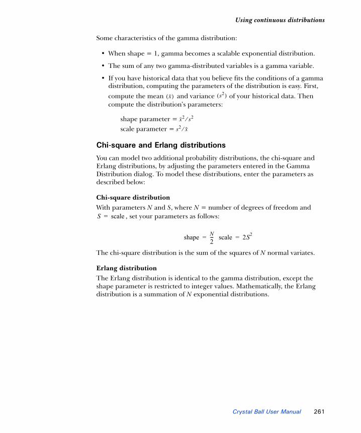
Using continuous distributions1
Some characteristics of the gamma distribution:
• When shape = 1, gamma becomes a scalable exponential distribution.
• The sum of any two gamma-distributed variables is a gamma variable.
• If you have historical data that you believe fits the conditions of a gamma distribution, computing the parameters of the distribution is easy. First, compute the mean and variance of your historical data. Then compute the distribution’s parameters:
shape parameter = scale parameter =
Chi-square and Erlang distributions
You can model two additional probability distributions, the chi-square and Erlang distributions, by adjusting the parameters entered in the Gamma Distribution dialog. To model these distributions, enter the parameters as described below:
Chi-square distributionWith parameters N and S, where N = number of degrees of freedom and
, set your parameters as follows:
The chi-square distribution is the sum of the squares of N normal variates.
Erlang distributionThe Erlang distribution is identical to the gamma distribution, except the shape parameter is restricted to integer values. Mathematically, the Erlang distribution is a summation of N exponential distributions.
x( ) s2( )
x2 s2⁄
s2 x⁄
S scale=
shape N2---= scale 2S2=
Crystal Ball User Manual 261

Appendix A | Selecting and Using Probability Distributions
Logistic distribution
Parameters
Mean, Scale
Description
The logistic distribution is commonly used to describe growth (i.e., the size of a population expressed as a function of a time variable). It can also be used to describe chemical reactions and the course of growth for a population or individual.
Figure A.9 Logistic distribution
Calculating parameters
There are two standard parameters for the logistic distribution: mean and scale. The mean parameter is the average value, which for this distribution is the same as the mode, since this is a symmetrical distribution.
After you select the mean parameter, you can estimate the scale parameter. The scale parameter is a number greater than 0. The larger the scale parameter, the greater the variance.
262 Crystal Ball User Manual

Using continuous distributions1
To calculate a more exact scale, you can estimate the variance and use the equation:
where is the scale parameter.
Lognormal distribution
Parameters
Mean, Standard Deviation
Conditions
The uncertain variable can increase without limits, but cannot fall below zero.
The uncertain variable is positively skewed with most of the values near the lower limit.
The natural logarithm of the uncertain variable yields a normal distribution.
Description
The lognormal distribution is widely used in situations where values are positively skewed, for example in financial analysis for security valuation or in real estate for property valuation.
Stock prices are usually positively skewed, rather than normally (symmetrically) distributed. Stock prices exhibit this trend because they cannot fall below the lower limit of zero, but might increase to any price without limit.
Similarly, real estate prices illustrate positive skewness since property values cannot become negative.
Example
The lognormal distribution can be used to model the price of a particular stock. You purchase a stock today at $50. You expect that the stock will be worth $70 at the end of the year. If the stock price
α 3 variance⋅
π2---------------------------=
α
Glossary Term: skewed, positively— A distribution in which most of the values occur at the lower end of the range.
Crystal Ball User Manual 263

Appendix A | Selecting and Using Probability Distributions
drops at the end of the year, rather than appreciating, you know that the lowest value it can drop to is $0.
On the other hand, the stock could end up with a price much higher than expected, thus implying no upper limit on the rate of return. In summary, your losses are limited to your original investment, but your gains are unlimited.
Using historical data, you can determine that the standard deviation of the stock’s price is $12.
Statistical Note: If you have historical data available with which to define a lognormal distribution, it is important to calculate the mean and standard deviation of the logarithms of the data and then enter these log parameters using the Parameters menu (Log Mean and Log Standard Deviation). Calculating the mean and standard deviation directly on the raw data will not give you the correct lognormal distribution. Alternatively, use the distribution fitting feature described on page 27.
The first step in selecting a probability distribution is matching your data with a distribution’s conditions. Checking the lognormal distribution:
• The price of the stock is unlimited at the upper end but cannot drop below $0.
• The distribution of the stock price is positively skewed.
• The natural logarithm of the stock price yields a normal distribution.
These conditions match those of the lognormal distribution (Figure A.10).
264 Crystal Ball User Manual

Using continuous distributions1
Figure A.10 Lognormal distribution
In the lognormal distribution, the mean parameter is set at $70.00 and the standard deviation set at $12.00. This distribution shows the probability that the stock price will be $x.
Lognormal parameter sets
By default, the lognormal distribution uses the arithmetic mean and standard deviation. For applications where historical data are available, it is more appropriate to use the logarithmic mean and logarithmic standard deviation or the geometric mean and geometric standard deviation. These options are available from the Parameters menu in the menubar.
For more information on these alternate parameters, see “Lognormal distribution” in the “Equations and Methods” chapter of the online Crystal Ball Reference Manual. For more information about this menu, see “Alternate parameter sets” on page 25.
Maximum extreme distribution
Parameters
Likeliest, Scale
Crystal Ball User Manual 265

Appendix A | Selecting and Using Probability Distributions
Description
The maximum extreme distribution is commonly used to describe the largest value of a response over a period of time: for example, in flood flows, rainfall, and earthquakes. Other applications include the breaking strengths of materials, construction design, and aircraft loads and tolerances. The maximum extreme distribution is also known as the Gumbel distribution. This distribution is closely related to the minimum extreme distribution, described beginning on page 267.
Figure A.11 Maximum extreme distribution
Calculating parameters
There are two standard parameters for the maximum extreme value distribution: Likeliest and Scale. The Likeliest parameter is the most likely value for the variable (the highest point on the probability distribution, or mode).
After you select the Likeliest parameter, you can estimate the Scale parameter. The Scale parameter is a number greater than 0. The larger the Scale parameter, the greater the variance.
To calculate a more exact scale, you can estimate the mean and use the equation:
α mean mode–0.57721
--------------------------------=
266 Crystal Ball User Manual

Using continuous distributions1
where is the Scale parameter.
Or estimate the variance and use the equation:
where is the Scale parameter.
Minimum extreme distribution
Parameters
Likeliest, Scale
Description
The minimum extreme distribution is commonly used to describe the smallest value of a response over a period of time: for example, rainfall during a drought. This distribution is closely related to the maximum extreme distribution, described beginning on page 265.
Figure A.12 Minimum extreme distribution
α
α 6 variance⋅π2
---------------------------=
α
Crystal Ball User Manual 267

Appendix A | Selecting and Using Probability Distributions
Calculating parameters
There are two standard parameters for the minimum extreme value distribution: Likeliest and Scale. The Likeliest parameter is the most likely value for the variable (the highest point on the probability distribution, or mode).
After you select the Likeliest parameter, you can estimate the Scale parameter. The Scale parameter is a number greater than 0. The larger the Scale parameter, the greater the variance.
To calculate a more exact scale, you can estimate the mean and use the equation:
where is the Scale parameter.
Or estimate the variance and use the equation:
where is the Scale parameter.
Normal distribution
Parameters
Mean, Standard Deviation
Conditions
Some value of the uncertain variable is the most likely (the mean of the distribution).
The uncertain variable could as likely be above the mean as it could be below the mean (symmetrical about the mean).
The uncertain variable is more likely to be in the vicinity of the mean than far away.
α mean mode–0.57721
--------------------------------=
α
α 6 variance⋅
π2---------------------------=
α
268 Crystal Ball User Manual
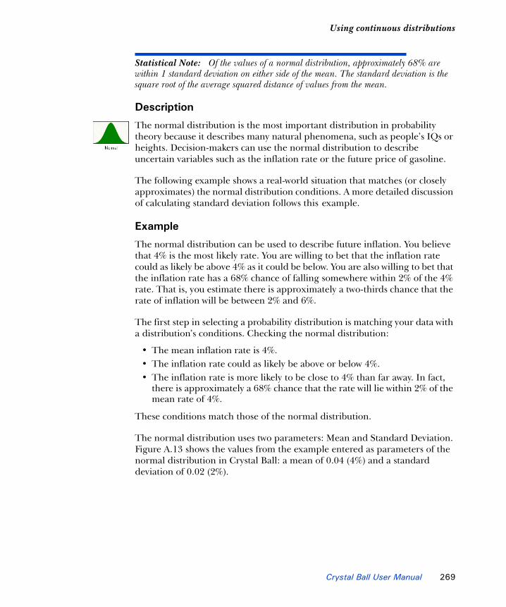
Using continuous distributions1
Statistical Note: Of the values of a normal distribution, approximately 68% are within 1 standard deviation on either side of the mean. The standard deviation is the square root of the average squared distance of values from the mean.
Description
The normal distribution is the most important distribution in probability theory because it describes many natural phenomena, such as people’s IQs or heights. Decision-makers can use the normal distribution to describe uncertain variables such as the inflation rate or the future price of gasoline.
The following example shows a real-world situation that matches (or closely approximates) the normal distribution conditions. A more detailed discussion of calculating standard deviation follows this example.
Example
The normal distribution can be used to describe future inflation. You believe that 4% is the most likely rate. You are willing to bet that the inflation rate could as likely be above 4% as it could be below. You are also willing to bet that the inflation rate has a 68% chance of falling somewhere within 2% of the 4% rate. That is, you estimate there is approximately a two-thirds chance that the rate of inflation will be between 2% and 6%.
The first step in selecting a probability distribution is matching your data with a distribution’s conditions. Checking the normal distribution:
• The mean inflation rate is 4%.• The inflation rate could as likely be above or below 4%. • The inflation rate is more likely to be close to 4% than far away. In fact,
there is approximately a 68% chance that the rate will lie within 2% of the mean rate of 4%.
These conditions match those of the normal distribution.
The normal distribution uses two parameters: Mean and Standard Deviation. Figure A.13 shows the values from the example entered as parameters of the normal distribution in Crystal Ball: a mean of 0.04 (4%) and a standard deviation of 0.02 (2%).
Crystal Ball User Manual 269
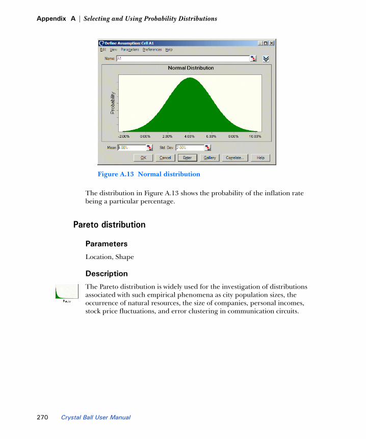
Appendix A | Selecting and Using Probability Distributions
Figure A.13 Normal distribution
The distribution in Figure A.13 shows the probability of the inflation rate being a particular percentage.
Pareto distribution
Parameters
Location, Shape
Description
The Pareto distribution is widely used for the investigation of distributions associated with such empirical phenomena as city population sizes, the occurrence of natural resources, the size of companies, personal incomes, stock price fluctuations, and error clustering in communication circuits.
270 Crystal Ball User Manual

Using continuous distributions1
Figure A.14 Pareto distribution
Calculating parameters
There are two standard parameters for the Pareto distribution: Location and Shape. The Location parameter is the lower bound for the variable.
After you select the Location parameter, you can estimate the Shape parameter. The Shape parameter is a number greater than 0, usually greater than 1. The larger the Shape parameter, the smaller the variance and the thicker the right tail of the distribution appears.
To calculate a more exact shape, you can estimate the mean and use the equation (for shapes greater than 1):
where is the Shape parameter and L is the Location parameter. You can use Excel Solver to help you calculate this parameter, setting the constraint of
>1.
Or estimate the variance and use the equation (for shapes greater than 2):
mean β L⋅β 1–------------=
β
β
variance β L2⋅β 2–( ) β 1–( )2
-------------------------------------=
Crystal Ball User Manual 271

Appendix A | Selecting and Using Probability Distributions
where is the Shape parameter and L is the Location parameter. You can use Excel Solver to help you calculate this parameter, setting the constraint of
>2.
Student’s t distribution
Parameters
Midpoint, Scale, Degrees of Freedom
Conditions
The values are distributed symmetrically about the midpoint.
The likelihood of values at the extreme ends is greater than those of the normal distribution.
Description
In classical statistics, the Student’s t distribution is used to describe the mean statistic for small sets of empirical data when the population variance is unknown. Classically, degrees of freedom is typically defined as the sample size minus 1.
For purposes of simulation, the Student’s t distribution resembles a normal curve, but with thicker tails (more outliers) and greater peakedness (high kurtosis) in the central region. As degrees of freedom increase (at around 30), the distribution approximates the normal distribution. For degrees of freedom larger than 30, you should use the normal distribution instead. The Student's t is a continuous probability distribution.
Since the Student’s t distribution has an additional parameter than controls the shape of the distribution (Degrees of Freedom) over the normal distribution, the greater flexibility of the Student’s t distribution is sometimes preferred for more precise modeling of nearly normal quantities found in many econometric and financial applications.
The default parameters for the Student's t distribution are Midpoint, Scale, and Degrees of Freedom.
β
β
272 Crystal Ball User Manual

Using continuous distributions1
Figure A.15 Student’s t distribution
The Midpoint parameter is the central location of the distribution (also mode), the x-axis value where you want to place the peak of the distribution. The Degrees of Freedom parameter controls the shape of the distribution. Smaller values result in thicker tails and less mass in the center. The Scale parameter affects the width of the distribution by increasing the variance without affecting the overall shape and proportions of the curve. Scale can be used to widen the curve for easier reading and interpretation. For example, if the midpoint were a large number, say 5000, the scale could be proportionately larger than if the midpoint were 500.
Example
For examples, see “Normal distribution” on page 268. The uses are the same except that the sample degrees of freedom will be < 30 for the Student’s t distribution.
Crystal Ball User Manual 273

Appendix A | Selecting and Using Probability Distributions
Triangular distribution
Parameters
Minimum, Likeliest, Maximum
Conditions
The minimum number of items is fixed.
The maximum number of items is fixed.
The most likely number of items falls between the minimum and maximum values, forming a triangular-shaped distribution, which shows that values near the minimum and maximum are less likely to occur than those near the most likely value.
Description
The triangular distribution describes a situation where you know the minimum, maximum, and most likely values to occur. For example, you could describe the number of cars sold per week when past sales show the minimum, maximum, and usual number of cars sold.
Example one
An owner needs to describe the amount of gasoline sold per week by his filling station. Past sales records show that a minimum of 3,000 gallons to a maximum of 7,000 gallons are sold per week, with most weeks showing sales of 5,000 gallons.
The first step in selecting a probability distribution is matching your data with a distribution’s conditions. Checking the triangular distribution:
• The minimum number of gallons is 3,000.
• The maximum number of gallons is 7,000.
• The most likely number of gallons (5,000) falls between 3,000 and 7,000, forming a triangle.
These conditions match those of the triangular distribution.
The triangular distribution has three parameters: Minimum, Likeliest, and Maximum. The conditions outlined in this example contain the values for these parameters: 3,000 (Minimum), 5,000 (Likeliest), and 7,000 (Maximum).
274 Crystal Ball User Manual

Using continuous distributions1
You would enter these values as the parameters of the triangular distribution in Crystal Ball.
The following triangular distribution shows the probability of x number of gallons being sold per week.
Figure A.16 Triangular distribution
Example two
The triangular distribution also could be used to approximate a computer-controlled inventory situation. The computer is programmed to keep an ideal supply of 25 items on the shelf, not to let inventory ever drop below 10 items, and not to let it ever rise above 30 items.
Check the triangular distribution conditions:
• The minimum inventory is 10 items.
• The maximum inventory is 30 items.
• The ideal level most frequently on the shelf is 25 items.
These conditions match those of the triangular distribution.
The result would be a distribution showing the probability of x number of items in inventory.
Crystal Ball User Manual 275

Appendix A | Selecting and Using Probability Distributions
Uniform distribution
Parameters
Minimum, Maximum
Conditions
The minimum value is fixed.
The maximum value is fixed.
All values between the minimum and maximum occur with equal likelihood.
Description
In the uniform distribution, all values between the minimum and maximum occur with equal likelihood.
Example one
An investment company interested in purchasing a parcel of prime commercial real estate wants to describe the appraised value of the property. The company expects an appraisal of at least $500,000 but not more than $900,000. They believe that all values between $500,000 and $900,000 have the same likelihood of being the actual appraised value.
The first step in selecting a probability distribution is matching your data with a distribution’s conditions. In this case:
• The minimum value is $500,000.
• The maximum value is $900,000.
• All values between $500,000 and $900,000 are equally possible.
These conditions match those of the uniform distribution. The uniform distribution has two parameters: the Minimum ($500,000) and the Maximum ($900,000). You would enter these values as the parameters of the uniform distribution in Crystal Ball.
276 Crystal Ball User Manual

Using continuous distributions1
Figure A.17 Uniform distribution
The distribution in Figure A.17 shows that all values between $500,000 and $900,000 are equally possible.
Example two
A manufacturer determines that he must receive 10% over production costs—or a minimum of $3 per unit—to make the manufacturing effort worthwhile. He also wants to set the maximum price for the product at $6 per unit, so that he can gain a sales advantage by offering the product for less than his nearest competitor. All values between $3 and $6 per unit have the same likelihood of being the actual product price.
The first step in selecting a probability distribution is matching your data with a distribution’s conditions. Checking the uniform distribution:
• The minimum value is $3 per unit.
• The maximum value is $6 per unit.
• All values between $3 and $6 are equally possible.
You would enter these values in Crystal Ball to produce a uniform distribution showing that all values from $3 to $6 occur with equal likelihood.
Crystal Ball User Manual 277

Appendix A | Selecting and Using Probability Distributions
Weibull distribution (also Rayleigh distribution)
Parameters
Location, Scale, Shape
Description
The Weibull distribution describes data resulting from life and fatigue tests. It is commonly used to describe failure time in reliability studies, and the breaking strengths of materials in reliability and quality control tests. Weibull distributions are also used to represent various physical quantities, such as wind speed.
The Weibull distribution is a family of distributions that can assume the properties of several other distributions. For example, depending on the shape parameter you define, the Weibull distribution can be used to model the exponential and Rayleigh distributions, among others.
The Weibull distribution is very flexible. When the Weibull Shape parameter is equal to 1.0, the Weibull distribution is identical to the exponential distribution. The Weibull Location parameter lets you set up an exponential distribution to start at a location other than 0.0. When the Shape parameter is less than 1.0, the Weibull distribution becomes a steeply declining curve. A manufacturer might find this effect useful in describing part failures during a burn-in period.
Figure A.18 Weibull distribution
278 Crystal Ball User Manual

Using continuous distributions1
When the Shape parameter is equal to 2.0, as in Figure A.18, a special form of the Weibull distribution, called the Rayleigh distribution, results. A researcher might find the Rayleigh distribution useful for analyzing noise problems in communication systems or for use in reliability studies.
Calculating parameters
There are three standard parameters for the Weibull distribution: Location, Scale, and Shape. The Location parameter is the lower bound for the variable.
The Shape parameter is a number greater than 0, usually a small number less than 10. When the Shape parameter is less than 3, the distribution becomes more and more positively skewed until it starts to resemble an exponential distribution (shape < 1). At a shape of 3.25, the distribution is symmetrical, and above that value, the distribution becomes more narrow and negatively skewed.
After you select the Location and Shape parameter, you can estimate the Scale parameter. The larger the scale, the larger the width of the distribution.
To calculate a more exact scale, estimate the mean and use the equation:
where α is the scale, β is the shape, L is the location, and Γ is the gamma function. You can use the Excel GAMMALN function and Excel Solver to help you calculate this parameter.
Statistical Note: For this distribution, there is a 63% probability that x falls between α and α+L.
Or estimate the mode and use the equation:
where α is the scale, β is the shape, and L is the location.
α mean L–
Γ 1 1β---+⎝ ⎠
⎛ ⎞----------------------=
α mode L–
1 1β---–⎝ ⎠
⎛ ⎞1β---
----------------------=
Crystal Ball User Manual 279

Appendix A | Selecting and Using Probability Distributions
Example
A lawn mower company is testing its gas-powered, self-propelled lawn mowers. They run 20 mowers, and keep track of how many hours each mower runs until its first breakdown. They use a Weibull distribution to describe the number of hours until the first failure.
Using discrete distributionsDiscrete probability distributions describe distinct values, usually integers, with no intermediate values and are shown as a series of vertical bars, such as the binomial distribution at the bottom of Figure A.4 on page 248. A discrete distribution, for example, might describe the number of heads in four flips of a coin as 0, 1, 2, 3, or 4.
The following discrete distributions are described later in this section in alphabetical order. Page references appear below the names.
Table A.3 Summary of discrete distributions
Shape Name Summary
Binomial(page 281)
The binomial distribution describes the number of times a particular event occurs in a fixed number of trials, such as the number of heads in 10 flips of a coin or the number of defective items in 50 items.
Discrete uniform(Basic)(page 283)
In the discrete uniform distribution, all integer values between the minimum and maximum are equally likely to occur. It is the discrete equivalent of the continuous uniform distribution.
Geometric(page 285)
The geometric distribution describes the number of trials until the first successful occurrence, such as the number of times you need to spin a roulette wheel before you win.
Hypergeometric(page 286)
The hypergeometric distribution is similar to the binomial distribution; both describe the number of times a particular event occurs in a fixed number of trials. However, binomial distribution trials are independent, while hypergeometric distribution trials change the success rate for each subsequent trial and are called “trials without replacement.”
Negative binomial(page 289)
The negative binomial distribution is useful for modeling the distribution of the number of trials until the r th successful occurrence, such as the number of sales calls you need to make to close a total of 10 orders. It is essentially a super-distribution of the geometric distribution.
Poisson(page 291)
The Poisson distribution describes the number of times an event occurs in a given interval, such as the number of telephone calls per minute or the number of errors per page in a document.
280 Crystal Ball User Manual

Using discrete distributions1
Binomial distribution
Parameters
Probability, Trials
Statistical Note: The word “trials,” as used to describe a parameter of the binomial distribution, is different from “trials” as it is used when running a simulation in Crystal Ball. Binomial distribution trials describe the number of times a given experiment is repeated (flipping a coin 50 times would be 50 binomial trials). A simulation trial describes a set of 50 coin flips (10 simulation trials would simulate flipping 50 coins 10 times).
Conditions
For each trial, only two outcomes are possible.
The trials are independent. What happens in the first trial does not affect the second trial, and so on.
The probability of an event occurring remains the same from trial to trial.
Description
The binomial distribution describes the number of times a particular event occurs in a fixed number of trials, such as the number of heads in 10 flips of a coin or the number of defective items in 50 items.
Example one
You want to describe the number of defective items in a total of 50 manufactured items, 7% of which (on the average) were found to be defective during preliminary testing.
Yes-no(Basic)(page 293)
The yes-no distribution is a discrete distribution that describes a set of observations that can have only one of two values, such as yes or no, success or failure, true or false, or heads or tails.
Table A.3 Summary of discrete distributions (Continued)
Shape Name Summary
Crystal Ball User Manual 281

Appendix A | Selecting and Using Probability Distributions
The first step in selecting a probability distribution is matching your data with a distribution’s conditions. Checking the binomial distribution:
• There are only two possible outcomes: the manufactured item is either good or defective.
• The trials (50) are independent of one another. Any given manufactured item is either defective or not, independent of the condition of any of the others.
• The probability of a defective item (7%) is the same each time an item is tested.
These conditions match those of the binomial distribution.
The parameters for the binomial distribution are Probability and Trials. In example one, the values for these parameters are 50 (Trials) and 0.07 (7% Probability of producing defective items). You would enter these values to specify the parameters of the binomial distribution in Crystal Ball.
Figure A.19 Binomial distribution
The distribution illustrated in Figure A.19 shows the probability of producing x number of defective items.
Example two
A company’s sales manager wants to describe the number of people who prefer the company’s product. The manager conducted a survey of 100
282 Crystal Ball User Manual

Using discrete distributions1
consumers and determined that 60% prefer the company’s product over the competitor’s.
Again, the conditions fit the binomial distribution with two important values: 100 (trials) and 0.6 (60% probability of success). These values specify the parameters of the binomial distribution in Crystal Ball. The result would be a distribution of the probability that x number of people prefer the company’s product.
Discrete uniform distribution
Parameters
Minimum, Maximum
Conditions
The minimum value is fixed.
The maximum value is fixed.
All integer values between the minimum and maximum are equally likely to occur.
Description
In the discrete uniform distribution, all integer values between the minimum and maximum are equally likely to occur. It is a discrete probability distribution. The discrete uniform distribution is very similar to the uniform distribution (page 276) except it is discrete instead of continuous; all its values must be integers.
The discrete uniform distribution can be used to model rolling a six-sided die. In that case, the minimum value would be 1 and the maximum 6.
Crystal Ball User Manual 283

Appendix A | Selecting and Using Probability Distributions
Figure A.20 Discrete uniform distribution
Example
A manufacturer determines that he must receive 10% over production costs—or a minimum of $5 per unit—to make the manufacturing effort worthwhile. He also wants to set the maximum price for the product at $15 per unit, so that he can gain a sales advantage by offering the product for less than his nearest competitor. All values between $5 and $15 per unit have the same likelihood of being the actual product price, however he wants to limit the price to whole dollars.
The first step in selecting a probability distribution is matching your data with a distribution’s conditions. Checking the uniform distribution:
• The minimum value is $5 per unit.
• The maximum value is $15 per unit.
• All integer values between $5 and $15 are equally possible.
You would enter these values in Crystal Ball to produce a discrete uniform distribution showing that all whole dollar values from $5 to $15 occur with equal likelihood. Figure A.20 illustrates this scenario.
284 Crystal Ball User Manual

Using discrete distributions1
Geometric distribution
Parameter
Probability
Conditions
The number of trials is not fixed.
The trials continue until the first success.
The probability of success is the same from trial to trial.
Description
The geometric distribution describes the number of trials until the first successful occurrence, such as the number of times you need to spin a roulette wheel before you win.
Example one
If you are drilling for oil and want to describe the number of dry wells you would drill before the next producing well, you would use the geometric distribution. Assume that in the past you have hit oil about 10% of the time.
The first step in selecting a probability distribution is matching your data with a distribution’s conditions. Checking the geometric distribution:
• The number of trials (dry wells) is unlimited.
• You continue to drill wells until you hit the next producing well.
• The probability of success (10%) is the same each time you drill a well.
These conditions match those of the geometric distribution.
The geometric distribution has only one parameter: Probability. In this example, the value for this parameter is 0.10, representing the 10% probability of discovering oil. You would enter this value as the parameter of the geometric distribution in Crystal Ball.
The distribution illustrated in Figure A.21 shows the probability of x number of wells drilled before the next producing well.
Crystal Ball User Manual 285

Appendix A | Selecting and Using Probability Distributions
Figure A.21 Geometric distribution
Example two
An insurance company wants to describe the number of claims received until a “major” claim arrives. Records show that 6% of the submitted claims are equal in dollar amount to all the other claims combined.
Again, identify and enter the parameter values for the geometric distribution in Crystal Ball. In this example, the conditions show one important value: a 0.06 (6%) probability of receiving that “major” claim. The result would be a distribution showing the probability of x number of claims occurring between “major” claims.
Hypergeometric distribution
Parameters
Success, Trials, Population
Statistical Note: The word “trials,” as used to describe a parameter of the hypergeometric distribution, is different from “trials” as it is used when running a simulation in Crystal Ball. Hypergeometric distribution trials describe the number of times a given experiment is repeated (removing 20 manufactured parts from a box would be 20 hypergeometric trials). A simulation trial describes the removing of 20 parts (10 simulation trials would simulate removing 20 manufactured parts 10 times).
286 Crystal Ball User Manual

Using discrete distributions1
Conditions
The total number of items or elements (the population size) is a fixed number: a finite population. The population size must be less than or equal to 1000.
The sample size (the number of trials) represents a portion of the population.
The known initial success rate in the population changes slightly after each trial.
Description
The hypergeometric distribution is similar to the binomial distribution in that both describe the number of times a particular event occurs in a fixed number of trials. The difference is that binomial distribution trials are independent, while hypergeometric distribution trials change the success rate for each subsequent trial and are called “trials without replacement.”
For example, suppose a box of manufactured parts is known to contain some defective parts. You choose a part from the box, find it is defective, and remove the part from the box. If you choose another part from the box, the probability that it is defective is somewhat lower than for the first part because you have removed a defective part. If you had replaced the defective part, the probabilities would have remained the same, and the process would have satisfied the conditions for a binomial distribution.
Example one
You want to describe the number of consumers in a fixed population who prefer Brand X. You are dealing with a total population of 40 consumers, of which 30 prefer Brand X and 10 prefer Brand Y. You survey 20 of those consumers.
The first step in selecting a probability distribution is matching your data with a distribution’s conditions. Checking the hypergeometric distribution:
• The population size (40) is fixed.
• The sample size (20 consumers) represents a portion of the population.
• Initially, 30 of 40 consumers preferred Brand X so the initial success rate is 30. This rate changes each time you question one of the 20 consumers, depending on the preference of the previous consumer.
The conditions in this example match those of the hypergeometric distribution.
Crystal Ball User Manual 287

Appendix A | Selecting and Using Probability Distributions
Statistical Note: If you have a probability from a different-sized sample instead of a success rate, you can estimate initial success by multiplying the population size by the probability of success. In this example, the probability of success is 75% (.75 x 40 = 30 and 30/40 = .75).
The three parameters of this distribution are initial Success, number of Trials, and Population size. The conditions outlined in this example contain the values for these parameters: a population Size of 40, sample size (Trials) of 20, and initial Success of 30 (30 of 40 consumers will prefer Brand X). You would enter these values as the parameters of the hypergeometric distribution in Crystal Ball.
Figure A.22 Hypergeometric distribution
The distribution illustrated in Figure A.22 shows the probability that x number of consumers prefer Brand X.
Example two
The U.S. Department of the Interior wants to describe the movement of wild horses in Nevada. Researchers in the department travel to a particular area in Nevada to tag 100 horses in a total population of 1,000. Six months later the researchers return to the same area to find out how many horses remained in the area. The researchers look for tagged horses in a sample of 200.
Check the data against the conditions of the hypergeometric distribution. The parameter values for the hypergeometric distribution in Crystal Ball are the population size of 1,000, sample size of 200, and an initial success rate of 100
288 Crystal Ball User Manual

Using discrete distributions1
out of 1,000 (or a probability of 10% — 0.1 — of finding tagged horses. The result would be a distribution showing the probability of observing x number of tagged horses.
Crystal Ball Note: If you used this distribution in a model created in Crystal Ball 2000.x, you might notice slight data changes when running that model in the current version of Crystal Ball. This is because some rounding might occur when converting the probability parameter used in previous releases to the success parameter used in this version of Crystal Ball.
Negative binomial distribution
Parameters
Probability, Shape
Conditions
The number of trials is not fixed.
The trials continue until the r th success.
The probability of success is the same from trial to trial.
Statistical Note: The total number of trials needed will always be equal to or greater than r.
Description
The negative binomial distribution is useful for modeling the distribution of the number of trials until the r th successful occurrence, such as the number of sales calls you need to make to close a total of 10 orders. It is essentially a super-distribution of the geometric distribution.
Example
A manufacturer of jet engine turbines has an order to produce 50 turbines. Since about 20% of the turbines do not make it past the high-velocity spin test, the manufacturer will actually have to produce more than 50 turbines.
Matching these conditions with the negative binomial distribution:
• The number of turbines to produce (trials) is not fixed.
Crystal Ball User Manual 289

Appendix A | Selecting and Using Probability Distributions
• The manufacturer will continue to produce turbines until the 50th one has passed the spin test.
• The probability of success (80%) is the same for each test.
These conditions match those of the negative binomial distribution.
The negative binomial distribution has two parameters: Probability and Shape. The Shape parameter specifies the r th successful occurrence. In this example you would enter 0.8 for the Probability parameter (80% success rate of the spin test) and 50 for the Shape parameter (Figure A.23).
Figure A.23 Negative binomial distribution
Some characteristics of the negative binomial distribution:
• When Shape = 1, the negative binomial distribution becomes the geometric distribution.
• The sum of any two negative binomial distributed variables is a negative binomial variable.
• Another form of the negative binomial distribution, sometimes found in textbooks, considers only the total number of failures until the r th successful occurrence, not the total number of trials. To model this form of the distribution, subtract out r (the value of the shape parameter) from the assumption value using a formula in your worksheet.
290 Crystal Ball User Manual

Using discrete distributions1
Poisson distribution
Parameter
Rate
Conditions
The number of possible occurrences in any interval is unlimited.
The occurrences are independent. The number of occurrences in one interval does not affect the number of occurrences in other intervals.
The average number of occurrences must remain the same from interval to interval.
Description
The Poisson distribution describes the number of times an event occurs in a given interval, such as the number of telephone calls per minute or the number of errors per page in a document.
Example one
An aerospace company wants to determine the number of defects per 100 square yards of carbon fiber material when the defects occur an average of 8 times per 100 square yards.
The first step in selecting a probability distribution is matching your data with a distribution’s conditions. Checking the Poisson distribution:
• Any number of defects is possible within 100 square yards.
• The occurrences are independent of one another. The number of defects in the first 100 square yards does not affect the number of defects in the second 100 square yards.
• The average number of defects (8) remains the same for each 100 square yards.
These conditions match those of the Poisson distribution.
The Poisson distribution has only one parameter: Rate. In this example, the value for this parameter is 8 (defects). You would enter this value to specify the parameter of the Poisson distribution in Crystal Ball.
Crystal Ball User Manual 291

Appendix A | Selecting and Using Probability Distributions
Figure A.24 Poisson distribution
The distribution illustrated in Figure A.24 shows the probability of observing x number of defects in 100 square yards of the carbon fiber material.
Statistical Note: The size of the interval to which the rate applies, 100 square yards in this example, has no bearing on the probability distribution; the rate is the only key factor. If needed for modeling a situation, information on the size of the interval must be encoded in your spreadsheet formulas.
Example two
A travel agency wants to describe the number of calls it receives in 10 minutes. The average number of calls in 10 minutes is about 35.
Again, you begin by identifying and entering the values to set the parameters of the Poisson distribution in Crystal Ball. In this example, the conditions show one important value: 35 calls or a rate of 35. The result would be a distribution showing the probability of receiving x number of calls in 10 minutes.
292 Crystal Ball User Manual

Using discrete distributions1
Yes-no distribution
Parameter
Probability of Yes (1)
Conditions
The random variable can have only one of two values, for example, 0 and 1.
The mean is p, or probability (0 < p < 1).
Description
The yes-no distribution is also called the Bernoulli distribution in statistical textbooks. This distribution describes a set of observations that can have only one of two values, such as yes or no, success or failure, true or false, or heads or tails. It is a discrete probability distribution.
The yes-no distribution has one parameter, Probability of Yes (1).
Figure A.25 Yes-no distribution
Example
A machine shop produces complex high-tolerance parts with a .02 probability of failure and a .98 probability of success. If a single part is pulled from the line, Figure A.26 shows the probability that the part is good.
Crystal Ball User Manual 293

Appendix A | Selecting and Using Probability Distributions
Figure A.26 Probability of pulling a good part
Using the custom distributionIf none of the provided distributions fits your data, you can use the custom distribution to define your own. For example, a custom distribution can be especially helpful if different ranges of values have specific probabilities. You can create a distribution of one shape for one range of values and a different distribution for another range.
The following sections explain how to use the custom distribution and provide examples of its use.
Custom distributionWith Crystal Ball, you can use the custom distribution to represent a unique situation that cannot be described using other distribution types: you can describe a series of single values, discrete ranges, or continuous ranges. This section uses real-world examples to describe the custom distribution.
Crystal Ball Note: For summaries of the data entry rules used in the examples plus additional rules, see “Entering tables of data into custom distributions” beginning on page 306 and “Other important custom distribution notes” beginning on page 311.
294 Crystal Ball User Manual

Using the custom distribution1
Since it is easier to understand how the custom distribution works with a hands-on example, you might want to start Crystal Ball and use it to follow the examples. To follow the custom distribution examples, first create a new Excel workbook then select cells as specified.
Example oneBefore beginning example one, open the Custom Distribution dialog as follows:
1. Click cell D11.
2. Select Define > Define Assumption.
The Distribution Gallery dialog appears.
3. Click the All category to select it.
4. Scroll to find the custom distribution, then click it.
5. Click OK.
Crystal Ball displays the Define Assumption dialog.
Figure A.27 Define Assumption dialog for custom distributions
Using the custom distribution, a company can describe the probable retail cost of a new product. The company decides the cost could be $5, $8, or $10. In this example, you will use the custom distribution to describe a series of single values.
Crystal Ball User Manual 295

Appendix A | Selecting and Using Probability Distributions
To enter the parameters of this custom distribution:
1. Type 5 in the Value field and click Enter.
Since you do not specify a probability, Crystal Ball defaults to a relative probability of 1.00 for the value 5. A single value bar displays the value 5.00.
Statistical Note: Relative probability means that the sum of the probabilities does not have to add up to 1. So the probability for a given value is meaningless by itself; it makes sense only in relation to the total relative probability. For example, if the total relative probability is 3 and the relative probability for a given value is 1, the value has a probability of 0.33.
2. Type 8 in the Value field.
3. Click Enter.
Since you did not specify a probability, Crystal Ball defaults to a relative probability of 1.00 (displayed on the scale to the left of the Custom Distribution dialog) for the value 8. A second value bar represents the value 8.
4. Type 10 in the Value field.
5. Click Enter.
Crystal Ball displays a relative probability of 1.00 for the value 10. A third single value bar represents the value 10.
Figure A.28 shows the value bars for the values 5, 8, and 10, each with a relative probability of 1.00.
296 Crystal Ball User Manual

Using the custom distribution1
Figure A.28 Single values
Now, each value has a probability of 1. However, when you run the simulation, their total relative probability becomes 1.00 and the probability of each value is reset to .3333.
If you want to reset their probabilities before you run the simulation, follow these steps:
1. Click the bar with a value of 5.00.
Its value appears in the Value field.
2. Type the probability as the formula =1/3 in the Probability field and click Enter.
You could also enter a decimal — for example, 0.333333 — but the formula is more exact.
3. Follow steps 6 and 7 for the other two bars.
Crystal Ball rescales each value to a relative probability of 0.33 on the left side of the screen.
Crystal Ball User Manual 297

Appendix A | Selecting and Using Probability Distributions
Figure A.29 Single values with adjusted probabilities
Example twoBefore beginning example two, clear the values entered in example one as follows:
1. Right-click in the chart and choose Clear Distribution from the right-click menu.
In this example, you will use the custom distribution to describe a continuous range of values, since the unit cost can take on any value within the specified intervals.
1. Choose Parameters > Continuous Ranges to enter value ranges.
2. Enter the first range of values:
• Type 5 in the Minimum field.
• Type 15 in the Maximum field.
• Type .75 in the Probability field. This represents the total probability of all values within the range.
3. Click Enter.
Crystal Ball displays a continuous value bar for the range 5.00 to 15.00, as in Figure A.30, and returns the cursor to the Minimum field. Notice that the height of the range is 0.075. This represents the total probability divided by the width (number of units) in the range, 10.
298 Crystal Ball User Manual

Using the custom distribution1
Figure A.30 A continuous custom distribution
4. Enter the second range of values:
• Type 16 in the Minimum field.
• Type 21 in the Maximum field.
• Type .25 in the Probability field.
• Click Enter.
Crystal Ball displays a continuous value bar for the range 16.00 to 21.00. Its height is .050, equal to .25 divided by 5, the number of units in the range. Both ranges now appear in the Custom Distribution dialog (Figure A.31).
Crystal Ball User Manual 299

Appendix A | Selecting and Using Probability Distributions
Figure A.31 Custom distribution with two continuous ranges
You can change the probability and slope of a continuous range, as described in the following steps:
1. Click anywhere on the value bar for the range 16 to 21.
The value bar changes to a lighter shade.
2. Choose Parameters > Sloping Ranges.
Additional parameters appear in the Custom Distribution dialog.
Figure A.32 Sloping Range parameters, Custom Distribution dialog
3. Set the Height of Min. and Height of Max. equal to what currently appears in the chart, 0.05.
This can be an approximate value. The Height of Min. is the height of the range Minimum and the Height of Max. is the height of the range Maximum.
4. Click Enter.
The range returns to its original color and its height appears unchanged.
300 Crystal Ball User Manual
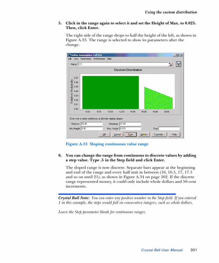
Using the custom distribution1
5. Click in the range again to select it and set the Height of Max. to 0.025. Then, click Enter.
The right side of the range drops to half the height of the left, as shown in Figure A.33. The range is selected to show its parameters after the change.
Figure A.33 Sloping continuous value range
6. You can change the range from continuous to discrete values by adding a step value. Type .5 in the Step field and click Enter.
The sloped range is now discrete. Separate bars appear at the beginning and end of the range and every half unit in between (16, 16.5, 17, 17.5 and so on until 21), as shown in Figure A.34 on page 302. If the discrete range represented money, it could only include whole dollars and 50-cent increments.
Crystal Ball Note: You can enter any positive number in the Step field. If you entered 1 in this example, the steps would fall on consecutive integers, such as whole dollars. Leave the Step parameter blank for continuous ranges.
Crystal Ball User Manual 301

Appendix A | Selecting and Using Probability Distributions
Figure A.34 A sloped discrete range with steps of .5
Although the bars have spaces between them, their heights and the width of the range they cover are equal to the previous continuous sloped range and the total probability is the same.
Crystal Ball Note: While a second continuous range could have extended from 15 to 20, the second range in this example starts at 16 rather than 15 to illustrate a discrete range because, unlike continuous ranges, discrete ranges cannot touch other ranges.
With Crystal Ball, you can enter single values, discrete ranges, or continuous ranges individually. You also can enter any combination of these three types in the same Custom Distribution dialog as long as you follow these guidelines: ranges and single values cannot overlap one another; however, the ending value of one continuous range can be the starting value of another continuous range.
Example threeThis example describes a special feature on the Custom Distribution dialog: the Load Data button, which lets you pull in numbers from a specified cell range (grouped data) on the worksheet. This example is not a hands-on exercise, but the illustrations will guide you through the procedure. After you read this section, you can experiment with your own data by pulling in numbers from specified cell ranges on your worksheet.
302 Crystal Ball User Manual

Using the custom distribution1
In this example, the same company decides that the unit cost of the new product can vary widely. The company feels it has a 20% chance of being any number between $10 and $20, a 10% chance of being any number between $20 and $30, a 30% chance of being any number between $40 and $50, a 30% chance of being a whole dollar amount between $60 and $80, and there is a 5% chance the value will be either $90 or $100. All the values have been entered on the worksheet in this order: range minimum value, range maximum value (for all but Single Value ranges), total probability, and step (for the Discrete Range only).
Figure A.35 Four-column custom data range
In this case, discrete ranges have the most parameters. So, you can create an assumption, choose Custom Distribution, and then choose Parameters > Discrete Ranges before loading the data.
Crystal Ball Note: If your data also included discrete sloping ranges, you could choose Parameters > Sloping Ranges before loading the data. The data table would then have five columns and could accommodate all data types.
Once the Parameters setting has been made, you can follow these steps to complete the data load:
1. Click the More button to the right of the Name field.
The Custom Distribution dialog expands to include a data table, as shown in Figure A.36.
Crystal Ball User Manual 303

Appendix A | Selecting and Using Probability Distributions
Figure A.36 Custom distribution with data table
A column appears for each parameter in the current set (selected using the Parameters menu). Parameters > Discrete Ranges was set before viewing the data table, so there is a column in the data table for each discrete range parameter. Because the single value and continuous ranges have subsets of the same group of parameters, their parameters will also fit into the table.
2. Since the values are already on the worksheet, you can click Load Data to enter them into the Custom Distribution dialog.
The Load Data dialog appears, as shown in Figure A.37.
Figure A.37 Load Data dialog, Custom Distribution
The default settings are appropriate for most purposes, but the following other options are available:
304 Crystal Ball User Manual

Using the custom distribution1
• When loading unlinked data, you can choose to replace the current distribution with the new data or append new data to the existing distribution.
• If probabilities are entered cumulatively into the spreadsheet you are loading, you can check Probabilities Are Cumulative. Then, Crystal Ball determines the probabilities for each range by subtracting the previous probability from the one entered for the current range. You will need to choose View > Cumulative Probability to display the data cumulatively in the assumption chart.
3. Enter a location range for your data. When all settings are correct, click OK.
Crystal Ball enters the values from the specified range into the custom distribution and plots the specified ranges, as shown in Figure A.38.
Figure A.38 Custom data from worksheet
Crystal Ball User Manual 305

Appendix A | Selecting and Using Probability Distributions
Entering tables of data into custom distributionsFollow the rules in this section for loading data.
Unweighted values
Single values are values that don’t define a range. Each value stands alone. For a series of single values with the same probabilities (unweighted values), use a one-column format or more than five columns. The values go in each cell and the relative probabilities are all assumed to be 1.0. Choose Parameters > Unweighted Values to enter these.
Figure A.39 Single values with the same probability
Figure A.40 Unweighted values loaded in a custom distribution
306 Crystal Ball User Manual
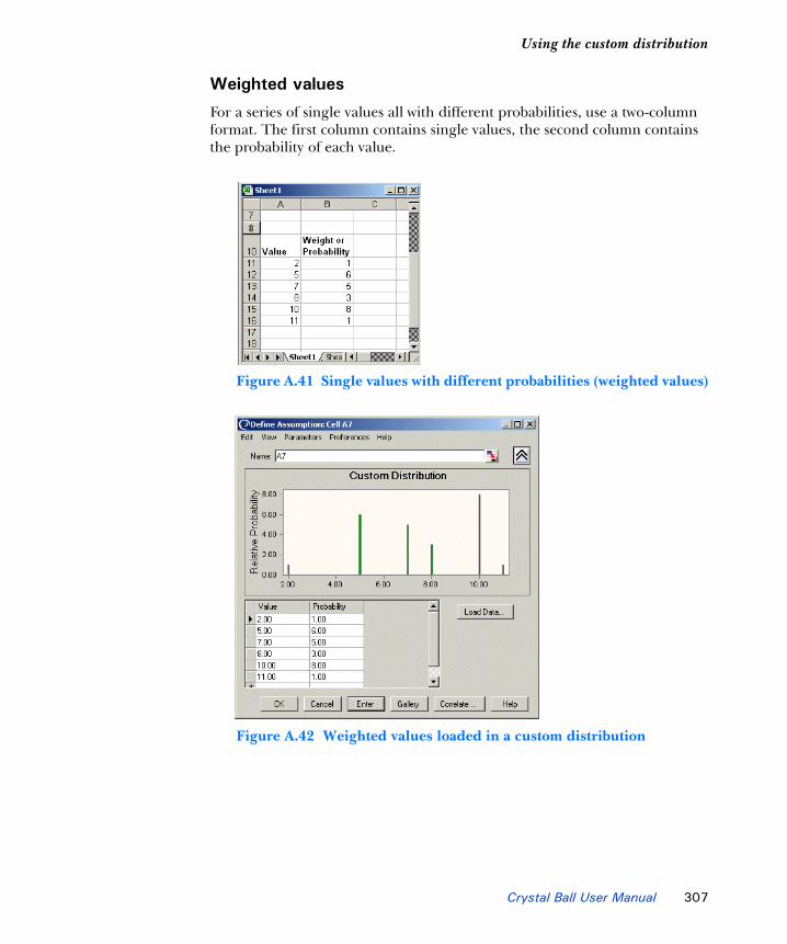
Using the custom distribution1
Weighted values
For a series of single values all with different probabilities, use a two-column format. The first column contains single values, the second column contains the probability of each value.
Figure A.41 Single values with different probabilities (weighted values)
Figure A.42 Weighted values loaded in a custom distribution
Crystal Ball User Manual 307

Appendix A | Selecting and Using Probability Distributions
Mixed single values, continuous ranges, and discrete ranges
For any mixture of single values and continuous ranges, use a three-column format, obtained by choosing Parameters > Continuous ranges. The three-column format is the same as using the first three columns shown in Figure A.36, Figure A.37, and Figure A.38 beginning on page 304.
If the mix includes uniform (non-sloping) discrete ranges, use a four-column format, as in the first four columns of Figure A.43 and Figure A.44. To obtain four columns, choose Parameters > Discrete Ranges.
Mixed ranges, including sloping ranges
If sloping ranges are included in a mix of ranges, choose Parameters > Sloping Ranges to display a five-column data table. The first column contains the range Minimum value, the second column contains the range Maximum value, the third column contains Height of Min. (the relative probability — height — at the Minimum value), the fourth column contains Height of Max. (the relative probability at the Maximum value), and the fifth column contains the Step value for discrete sloping ranges. For continuous sloping ranges the fifth column (Step) is left blank.
Note that if there are uniform discrete ranges, their first three columns contain the Minimum, Maximum, and Probability as in a four-column format but the fourth column is left blank and Step is entered in the fifth column.
Figure A.43 Mixed ranges, including sloping ranges
308 Crystal Ball User Manual
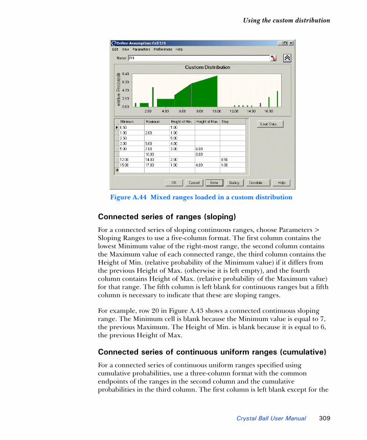
Using the custom distribution1
Figure A.44 Mixed ranges loaded in a custom distribution
Connected series of ranges (sloping)
For a connected series of sloping continuous ranges, choose Parameters > Sloping Ranges to use a five-column format. The first column contains the lowest Minimum value of the right-most range, the second column contains the Maximum value of each connected range, the third column contains the Height of Min. (relative probability of the Minimum value) if it differs from the previous Height of Max. (otherwise it is left empty), and the fourth column contains Height of Max. (relative probability of the Maximum value) for that range. The fifth column is left blank for continuous ranges but a fifth column is necessary to indicate that these are sloping ranges.
For example, row 20 in Figure A.43 shows a connected continuous sloping range. The Minimum cell is blank because the Minimum value is equal to 7, the previous Maximum. The Height of Min. is blank because it is equal to 6, the previous Height of Max.
Connected series of continuous uniform ranges (cumulative)
For a connected series of continuous uniform ranges specified using cumulative probabilities, use a three-column format with the common endpoints of the ranges in the second column and the cumulative probabilities in the third column. The first column is left blank except for the
Crystal Ball User Manual 309

Appendix A | Selecting and Using Probability Distributions
minimum value of the first range, beside the maximum in the second column. Be sure to check Probabilities Are Cumulative in the Load Data dialog.
Figure A.45 Connected continuous uniform ranges
Figure A.46 Connected continuous uniform ranges after loading
Other data load notes
You can load each type of range separately or you can specify the range type with the greatest number of parameters and load all types together. Other rules are.
• Cumulative probabilities are supported for all but sloping ranges.
• Blank probabilities are interpreted as a relative probability of 1.0.
• Ranges or values with 0 probabilities are removed. Sloping ranges with Height of Min. and Height of Max. equal to 0 are also removed.
• For continuous connected ranges, for either endpoint values or probabilities, if the starting cell is blank, the previous end value is used as the start for this range.
310 Crystal Ball User Manual
Using the custom distribution1
• When you load a discrete value that exists in the table already, its probability is incremented by 1. For continuous ranges, this is not allowed; an error message about overlapping ranges appears.
Changes from Crystal Ball 2000.x (5.x)In previous versions of Crystal Ball, discrete values with the same probability could be entered in ranges with five columns or more. Now, they cannot be entered in ranges with five columns but can only be entered in single columns or ranges with six or more columns (to distinguish them from sloping ranges).
In previous versions of Crystal Ball, continuous uniform ranges with cumulative probabilities could be entered in a two-column format. Now a three-column format is required, discussed in “Connected series of continuous uniform ranges (cumulative)” on page 309.
The three-column sloping range format used in previous versions of Crystal Ball has been replaced by a five-column format, described in “Mixed ranges, including sloping ranges” on page 308 and the section that follows it, “Connected series of ranges (sloping).”
Other important custom distribution notesEven if you don’t load data from the spreadsheet into the Custom Distribution dialog, you can still add and edit data using the data table. To do this, click the More button to display the data table. Then, you can:
• Enter a different value in the data table and click Enter to change the data.
• Type the minimum, maximum, probability, and step (if discrete data) into a blank row and click Enter to add new data.
• To delete a single range of data, select that row of data, right-click, and choose Delete Row.
• To clear all data rows, right-click within the data table and choose Clear Distribution.
• To delete a single range of data without using the data table, click the range to select it and either:
• Set the Probability or Height of Min. and Height of Max. to 0, or
• Choose Edit > Delete Row or right-click and choose Delete Row.
• Statistics for custom distributions are approximate.
Crystal Ball User Manual 311
Appendix A | Selecting and Using Probability Distributions
Truncating distributionsYou can change the bounds or limits of each distribution, except the custom distribution, by dragging the truncation grabbers or by entering different numeric endpoints for the truncation grabbers. This “truncates” the distribution. You can also exclude a middle area of a distribution by crossing over the truncation grabbers to “white out” the portion you want to exclude.
Crystal Ball Note: To display the truncation grabbers, open an assumption in the Define Assumption dialog and click the More button.
For example, suppose you want to describe the selling price of a house up for auction after foreclosure. The bank that holds the mortgage will not sell for less than $80,000. They expect the bids to be normally distributed around $100,000 with a standard deviation of $15,000. In Crystal Ball you would specify the mean as 100,000 and the standard deviation as 15,000 and then move the left grabber to set the limit of 80,000. The grabber “whites out” the portion you want to exclude, as shown in Figure A.47.
Be aware...Each adjustment changes the characteristics of the probability distribution. For example, the truncated normal distribution in Figure A.47 will no longer have an actual mean of $100,000 and standard deviation of $15,000. Also, statistics values will be approximate for truncated distributions.
When using alternate percentile parameters, the actual percentiles calculated for a truncated distribution will differ from the specified parameter values. For example, a normal distribution specified with 10th/90th percentiles and truncated on either side of the distribution will have actual 10th/90th percentiles greater or less than the specified percentiles.
Crystal Ball Note: Showing the mean line of the distribution is useful when truncating distributions. However, the mean line value might differ from the Mean parameter field. The mean line shows the actual mean of the truncated distribution while the Mean parameter field shows the mean of the complete distribution.
312 Crystal Ball User Manual

Comparing the distributions1
Figure A.47 Truncated distribution example
Comparing the distributionsMany of the distributions discussed in this chapter are related to one another in various ways. For example, the geometric distribution is related to the binomial distribution. The geometric distribution represents the number of trials until the next success while the binomial represents the number of successes in a fixed number of trials. Similarly, the Poisson distribution is related to the exponential distribution. The exponential distribution represents the amount of time until the next occurrence of an event while the Poisson distribution represents the number of times an event occurs within a given period of time.
In some situations, as when the number of trials for the binomial distribution becomes very large, the normal and binomial distributions become very similar. For these two distributions, as the number of binomial trials approaches infinity, the probabilities become identical for any given interval. For this reason, you can use the normal distribution to approximate the binomial distribution when the number of trials becomes too large for Crystal Ball to handle (more than 1000 trials). You also can use the Poisson distribution to approximate the binomial distribution when the number of trials is large, but there is little advantage to this since Crystal Ball takes a comparable amount of time to compute both distributions.
Crystal Ball User Manual 313

Appendix A | Selecting and Using Probability Distributions
Likewise, the normal and Student’s t distributions are related. With Degrees of Freedom > 30, Student’s t closely approximates the normal distribution.
The binomial and hypergeometric distributions are also closely related. As the number of trials and the population size increase, the hypergeometric trials tend to become independent like the binomial trials: the outcome of a single trial has a negligible effect on the probabilities of successive observations. The differences between these two types of distributions become important only when you are analyzing samples from relatively small populations. As with the Poisson and binomial distributions, Crystal Ball requires a similar amount of time to compute both the binomial and hypergeometric distributions.
The yes-no distribution is simply the binomial distribution with Trials = 1.
The Weibull distribution is very flexible. Actually, it consists of a family of distributions that can assume the properties of several distributions. When the Weibull shape parameter is 1.0, the Weibull distribution is identical to the exponential distribution. The Weibull location parameter lets you set up an exponential distribution to start at a location other than 0.0. When the shape parameter is less than 1.0, the Weibull distribution becomes a steeply declining curve. A manufacturer might find this effect useful in describing part failures during a burn-in period. When the shape parameter is equal to 2.0, a special form of the Weibull distribution, called the Rayleigh distribution, results. A researcher might find the Rayleigh distribution useful for analyzing noise problems in communication systems or for use in reliability studies. When the shape parameter is set to 3.25, the Weibull distribution approximates the shape of the normal distribution; however, for applications when the normal distribution is appropriate, us it instead of the Weibull distribution.
The gamma distribution is also a very flexible family of distributions. When the shape parameter is 1.0, the gamma distribution is identical to the exponential distribution. When the shape parameter is an integer greater than one, a special form of the gamma distribution, called the Erlang distribution, results. The Erlang distribution is especially useful in the areas of inventory control and queueing theory, where events tend to follow Poisson processes. Finally, when the shape parameter is an integer plus one half (e.g., 1.5, 2.5, etc.), the result is a chi-squared distribution, useful for modeling the effects between the observed and expected outcomes of a random sampling.
When no other distribution seems to fit your historical data or accurately describes an uncertain variable, you can use the custom distribution to simulate almost any distribution. The Load Data button on the Custom Distribution dialog lets you read a series of data points or ranges from value cells in your worksheet. If you like, you can use the mouse to individually alter
314 Crystal Ball User Manual

Using probability functions1
the probabilities and shapes of the data points and ranges so that they more accurately reflect the uncertain variable.
Using probability functionsFor each of the Crystal Ball distributions, there is an equivalent Excel function. You can enter these functions in your spreadsheet directly instead of defining distributions using the Define Assumption command. Be aware, though, that there are a number of limitations in using these functions. These are listed below.
To view these functions and their parameters, choose Insert > Function in Excel, be sure the category is set to All, and then scroll down to the list of functions that starts CB.
Figure A.48 Crystal Ball functions in Excel
Parameters and a brief description appear below the list of functions. The Cutoff parameters let you enter truncation values, while NameOf is the assumption name. For parameter descriptions and details on each distribution, see the entry for that distribution earlier in this appendix.
Crystal Ball Note: The beta distribution changed from previous versions to Crystal Ball 7. Both the original and revised functions appear for compatibility. CB.Beta has three parameters but CB.Beta2 is the Crystal Ball 7 version with Minimum and Maximum instead of Scale.
Crystal Ball User Manual 315
Appendix A | Selecting and Using Probability Distributions
Limitations of probability functionsDistributions defined with probability functions differ from those entered with the Define Assumption command in these ways:
• You can’t correlate them.
• You can’t view charts or statistics on them.
• You can’t extract data from them or include them in reports.
• They are not included in sensitivity analyses or charts.
Probability functions and random seeds“Sampling preferences” on page 83 describes how you can use the Sampling tab of the Run Preferences dialog to use the same sequence of random numbers for each simulation.
If you use Define > Define Assumption or the Define Assumption toolbar button to define assumptions, the same sequence of random numbers is used for each simulation, even if you switch from Extreme speed to Normal speed or back to Extreme speed. If you use the probability functions to define assumptions, one sequence of random numbers is used for Extreme speed and a different sequence is used for Normal speed.
316 Crystal Ball User Manual

Appendix BMaximizing Your Use of Crystal Ball
In this appendix• Simulation accuracy
• Simulation speed
• Sample size
• Correlated assumptions
This chapter contains information that you can use to improve the overall performance of Crystal Ball. These improvements occur in terms of the accuracy of your model or speed of the results.
Crystal Ball User Manual 317

Appendix B | Maximizing Your Use of Crystal Ball
Simulation accuracy
The accuracy of your simulation is primarily governed by two factors:
• The number of trials, or length, of the simulation
• The sampling method
Generally speaking, the more trials you run in a simulation, the greater the accuracy of the statistics and percentiles information. This greater accuracy comes at the expense of lengthier simulation times and higher memory usages (see later sections on simulation speed and memory usage). Also, for a given number of trials, the accuracy of the statistics and percentiles greatly depends on the shape and nature of the forecast distribution.
If you’re not sure how many trials to run for a specific level of accuracy, you can use Crystal Ball’s precision control feature (described below) to automatically determine the appropriate number of trials to run. For a detailed picture of simulation’s statistical accuracy, or simply if you’re curious, you can run the Bootstrap tool under the Run menu to generate a forecast chart for each statistic or percentile of interest.
The sampling method is the other primary factor governing simulation accuracy. During a simulation, Monte Carlo sampling generates natural, “what-if ” type scenarios while Latin Hypercube’s sampling is constrained, but more accurate. See page 321 for further discussion on sampling methods.
Precision controlThe precision control feature lets you set how precise you want the forecast statistics to be. Crystal Ball runs the simulation until the selected forecast statistics reach the required precision as determined by calculating confidence intervals.
Crystal Ball Note: See “Confidence intervals” in the “Statistical Definitions” chapter of the online Crystal Ball Reference Manual for more information about how Crystal Ball calculates confidence intervals.
Generally speaking, as more trials are calculated, the confidence intervals narrow and statistics become more precise. The precision control feature in Crystal Ball uses this characteristic of confidence intervals to determine when a specified precision of a statistic has been reached. It compares the specified precision to the confidence interval. When the calculated confidence interval drops to less than the specified precision, the simulation stops.
318 Crystal Ball User Manual

Simulation accuracy1
For each forecast, you can specify precision in either absolute terms in units of the forecast, or in relative terms as percentages. These settings are made on the Precision tab of the expanded Define Forecast dialog or the Forecast Preferences dialog. Each method, absolute or relative, has its own benefits and drawbacks.
Specifying precision in absolute terms can give you greater control of the simulation when the shape and scale of the forecast distribution is roughly known. For example, for a Gross Profit forecast (from the Vision Research model) that ranges from $25.5 to $64.0 million dollars, you can require the precision of the mean to be within plus or minus $100,000 or some other convenient measure of accuracy. However, with the same forecast range, an absolute accuracy of $1000 might require an unreasonably large number of trials to reach. So, the drawback of using absolute precision is that it might require experimentation to determine reasonable accuracy values.
Figure B.1 Absolute precision control example
Specifying precision in relative terms can give you greater control of the simulation when the shape and scale of the forecast distribution is largely unknown and you are interested in the accuracy only as it relates to the overall distribution itself. In the Gross Profit example above, you might not know or care if the distribution ranges from $25,500 to $64,000 dollars or from $25.5 to $64.0 million dollars. You might require only that the simulation's estimate of the mean fall within plus or minus 5% of itself.
Crystal Ball User Manual 319
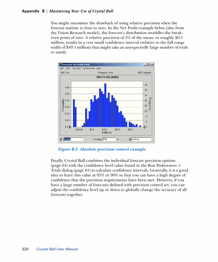
Appendix B | Maximizing Your Use of Crystal Ball
You might encounter the drawback of using relative precision when the forecast statistic is close to zero. In the Net Profit example below (also from the Vision Research model), the forecast’s distribution straddles the break-even point of zero. A relative precision of 5% of the mean, or roughly $0.5 million, results in a very small confidence interval (relative to the full range width of $49.1 million) that might take an unexpectedly large number of trials to satisfy.
Figure B.2 Absolute precision control example
Finally, Crystal Ball combines the individual forecast precision options (page 64) with the confidence level value found in the Run Preferences > Trials dialog (page 81) to calculate confidence intervals. Generally, it is a good idea to leave this value at 95% or 90% so that you can have a high degree of confidence that the precision requirements have been met. However, if you have a large number of forecasts defined with precision control set, you can adjust the confidence level up or down to globally change the accuracy of all forecasts together.
320 Crystal Ball User Manual

Simulation speed1
Sampling methodChoosing between Monte Carlo and Latin hypercube sampling affects how the random numbers are generated for the individual assumptions.
In almost all cases, Latin hypercube will produce more accurate forecast statistics (especially the mean) given the same number of trials as Monte Carlo since it is a more consistent sampling method. If you are primarily interested in the accuracy of your statistics, you should select Latin hypercube as the sampling method in the Run Preferences > Sampling dialog (page 83).
If you are primarily interested in evaluating how your spreadsheet model behaves under various “what-if ” scenarios, you should select Monte Carlo as the sampling method. Monte Carlo produces assumptions with the most randomness and hence will simulate real-life situations the best.
Simulation speedMonte Carlo simulations can be very time-consuming. You can change a number of factors that affect the speed of simulations. The factors are listed below in order of importance:
1. Change the Speed preferences.
In the Run Preferences > Speed dialog (page 84), there are options that can dramatically increase the speed of your simulation. Of course, if you have Crystal Ball Professional Edition or Premium Edition, you can run in Extreme speed, with dramatic cuts in run times.
If your model is incompatible with Extreme speed or you have Crystal Ball Standard Edition, you can, in increasing order of helpfulness:
• Redraw forecasts less often (available in Extreme speed).
• Update worksheets only every few seconds or so.
• Suppress chart windows during simulations (available in Extreme speed).
• Minimize Excel workbooks during simulations.
• Minimize Excel workbooks and suppress chart windows (the fastest combination of settings).
2. Use the precision control feature.
The precision control feature (page 81) can be used to either increase the precision of your simulations or increase the speed of your simulations. If you set the confidence level to a high number, your simulations will be
Crystal Ball User Manual 321

Appendix B | Maximizing Your Use of Crystal Ball
more precise, but might run significantly longer. However, if you do not need as precise a result, you can set the confidence level to a lower number and the simulation speed will increase.
Using this feature to speed up your model will require you to experiment with different confidence levels.
3. Reduce the size of the model by reducing the number of assumptions, forecasts, and correlations.
Large models require more time per trial. For example, a model that takes 3 or 4 seconds per recalculation cycle will take up to an hour to simulate 1,000 trials.
Greater numbers of assumptions and forecasts slow the simulation, especially if the assumptions and forecasts are scattered across many spreadsheets in your model. Start by examining the structure and nature of your model to locate possible efficiencies. You can also use the sensitivity feature or the Tornado Chart tool to determine which assumptions contribute the least amount of uncertainty to your most important forecasts. Freeze or eliminate the least important assumptions from the simulation.
Correlated assumptions can also consume a significant amount of processing time; the time grows geometrically as the number of correlated assumptions increases.
4. Reduce the use of other applications.
Quitting other applications and closing or minimizing windows can be helpful in reducing overhead and increasing simulation speed.
5. Increase your system’s RAM.
The amount of RAM in your computer has a large effect on the speed of simulations. Modern operating systems give applications such as spreadsheets the appearance of additional RAM through the use of virtual memory.
Virtual memory lets you run a greater number of applications than would otherwise be possible, but slows down overall processing speed because the system is frequently accessing the hard drive. If you hear your hard disk being used during a simulation, there might not be enough RAM to hold all parts of the simulation. Buying more RAM or turning off virtual memory (if possible) are solutions to this problem.
322 Crystal Ball User Manual

Sample size1
Sample sizeThe sample size option is located on the Run Preferences > Sampling dialog (page 83). Sample size, which is initially set to 500, affects Latin hypercube sampling. It divides each assumption’s distribution into a number of intervals of equal probability. The sample size governs the number of intervals for each distribution. Crystal Ball generates an assumption value for each interval according to the interval’s probability distribution.
While any sample size greater than 100 should produce sufficiently acceptable results, you can set this number higher to maximize accuracy. There is no absolute limit to sample size, although samples greater than 100,000 work best with at least 1 GB RAM and might take a long time to run. The increased accuracy resulting from the use of larger samples, however, requires additional memory. If memory becomes an issue, reduce the sample size and consider adding more RAM.
Correlated assumptionsThere is a practical limit of about 250 fully correlated assumptions (assumptions that are correlated to every other assumption) and up to about 1,000 serially correlated assumptions (assumptions that are correlated to one or two other assumptions) for each workbook. If you have a large number of correlated assumptions:
• For coefficients that are close to zero and are nearly independent, remove the correlation.
• For coefficients that are close to one, replace one of the assumptions with a formula in your spreadsheet.
If Crystal Ball detects inconsistently correlated assumptions when a simulation is running, it first determines whether small adjustments to the correlation coefficients are possible. This process might take a long time, depending on the number of correlated assumptions. Crystal Ball displays the message “Examining the Correlation Coefficients”. If you get this message, you should probably stop and redefine your correlations.
If small adjustments to the correlation coefficients are possible, a dialog appears, letting you decide whether to cancel the simulation or continue with the adjusted coefficients.
Select one of the following responses:
Crystal Ball User Manual 323

Appendix B | Maximizing Your Use of Crystal Ball
• Click Adjust Coefficients This Time Only to continue the simulation with the adjusted coefficients.
Since adjusted coefficients are not saved permanently, a dialog appears again if you stop and restart the simulation.
• To continue the simulation, replacing your original correlation coefficients with the adjusted ones, click Adjust Coefficients Permanently.
Crystal Ball Note: Correlation coefficients that were specified using a cell reference in place of an actual value are replaced with a permanent value (the cell references are removed).
• To terminate the simulation, click Cancel.
If small adjustments to the correlation coefficients are not possible, the simulation stops with an error message prompting you to reexamine your coefficients. To solve the problem, you can usually make large coefficients smaller or change your spreadsheet model to use formulas to calculate assumptions with large correlation coefficients. Creating a report containing just your assumptions might make it easier to spot problems.
324 Crystal Ball User Manual

Appendix CUsing the Extreme Speed Feature
In this appendix• Overview
• Compatibility issues
• Other important differences
• Numerical differences
• Maximizing the benefits of Extreme Speed
This appendix describes Extreme speed, a Speed preference available in Crystal Ball Professional and Premium editions that runs simulations up to 100 times faster than Normal speed.
Crystal Ball User Manual 325

Appendix C | Using the Extreme Speed Feature
OverviewExtreme speed, available only in Crystal Ball Professional and Premium editions, runs simulations up to 100 times faster than Normal speed. With Extreme speed, you won’t need to wait for simulation results or compromise on the number of trials you run. Extreme speed makes it more practical to use CB Tools that run multi-simulations or to seek optimal solutions with OptQuest in a reasonable length of time.
The Extreme Speed feature uses PSI Technology, a high-speed, Excel-compatible Polymorphic Spreadsheet Interpreter for running simulations on workbooks. This technology was developed by Frontline Systems, the maker of Excel’s Solver add-in. PSI Technology supports nearly all of the 320 standard Excel functions, including the financial, statistical, and engineering functions that are part of the Analysis Toolpak.
By default, Crystal Ball is set to use Extreme speed when initially loaded. If a model is not compatible with Extreme speed, a dialog offers the opportunity to downshift to Normal speed temporarily for that simulation. “Compatibility issues,” below, explains conditions that cause a model to be incompatible with Extreme speed. The simulation speed can be changed using the Speed tab in the Run Preferences dialogs (see “Speed preferences” on page 84 for details).
Compatibility issuesWhile Extreme speed can greatly decrease simulation run times, not all models are compatible with Extreme speed. When you start a simulation, Crystal Ball detects if your spreadsheet is compatible with Extreme speed and warns you if it is incompatible. If you choose, you can run the simulation in Normal speed using standard Excel, or you can change your spreadsheet model to correct the incompatibility.
This section lists functions and formula constructs that are not compatible with Extreme speed and suggests workarounds. Besides the issues listed below, some differences may also exist due to undocumented Excel behaviors, changes in the newest versions of Excel, and so on. Also, small differences in the last few decimal places of certain built-in function values should be expected, due to minor algorithmic differences in the way formulas might be computed.
It is important to note that incompatibilities in functions and formula constructs only concern the cells involved in the calculation of a forecast cell. If there are incompatibilities in cells that are not part of that calculation path, these are not detected and the simulation is allowed to run.
326 Crystal Ball User Manual

Compatibility issues1
Multiple-workbook modelsExtreme speed can now run simulations on multiple workbooks. If you are running in Extreme speed and the workbook contains external references to cells in other closed workbooks, Crystal Ball obtains the current value from those workbooks. References to cells in other open workbooks are dynamically updated if those cells depend on one or more assumptions. If the external reference is part of a formula (not a simple external reference), this is not compatible with Extreme speed:
• Example message: “Unable to interpret formula at cell location [Book1.xls]Sheet1!A1. (Code #5524 - Complex external reference)”
• Workaround: If possible, consolidate all of the variables and formulas from a multi-workbook model containing Crystal Ball data into a single workbook.
Circular referencesCircular references within a model are supported as long as Iteration is checked on the Tools > Options > Calculation tab in Excel. If Crystal Ball detects a circular reference and Iteration is not checked, this error appears:
• Example message: “Circular reference detected at cell [Book1.xls]Sheet1!A1. (Code #5523)”
• Workaround: Stop the simulation and check Iteration on the Tools > Options > Calculation tab.
Crystal Ball Note: In Extreme speed, circular references with short Iteration setting may not match Excel’s values because of differences in calculation algorithms. For most consistent results, set Iteration to at least 1,000.
However, if a circular reference is non-converging, its results can differ greatly when run at both Extreme and Normal speed, regardless of the Iteration setting. If a circular reference is non-converging, this error message appears:
• Example message: “Unable to run in Extreme speed for the following reason: Circular references do not converge, results cannot be guaranteed to match Normal speed. To bypass this message, turn off “Stop on calculation errors” in the Run Preferences dialog. (Code #5545)”
• Workaround: There is no workaround. Check the formulas in the workbook that have created this circular reference and look for a problem that keeps this circular reference from converging to a single value.
Crystal Ball User Manual 327

Appendix C | Using the Extreme Speed Feature
Crystal Ball Note: Simulations with circular references run in non-vectorized mode. For this reason, they will probably run more slowly than simulations without circular references.
Crystal Ball Excel functionsThe following Crystal Ball spreadsheet functions are handled normally:
CB.IterationsFN
distribution functions (such as CB.Binomial)
These functions are not supported in Extreme speed during a simulation:
CB.GetForeStatFN
CB.GetForePercentFN
CB.GetRunPrefsFN
CB.GetAssumPercentFN
CB.GetCertaintyFN
While running in Extreme speed, all values for these functions return #VALUE. At the end of the simulation, Crystal Ball performs a final recalculation on the model so these functions are evaluated properly. Normally, this should not present a problem unless one of these functions was defined as a forecast and you are expecting a valid value to be computed during the simulation. If one of these “Get” functions feeds into a forecast during a simulation, this is not compatible with Extreme speed:
• Example message: “Unsupported Excel or Crystal Ball function at cell location [Book1.xls]Sheet1!A1. (Code #5539)”
• Workaround: Defining forecasts on statistical functions that are dependent on other forecasts is generally not a good modeling practice. If you need to have a forecast cell defined on a statistical result from another forecast, use the Auto Extract feature for the dependent forecast instead of using one of the above Crystal Ball functions.
User-defined functionsCalls to user-defined or third-party functions are allowed. The functions may be written in Visual Basic or they may be in XLL or COM Automation DLL libraries that have been opened in Excel.
328 Crystal Ball User Manual
Compatibility issues1
Pure functions
To be compatible with Extreme Speed, user-defined functions must be “pure.” A “pure function" is one that computes its value solely on the basis of values passed to it as arguments. A function that is not “pure" might reference global data not passed as an argument. For example, it might get the value of a worksheet cell or a defined name and use this as an input to compute the function value. If the global data depends on the assumptions — if, for example, it is a worksheet cell with a formula computed from the assumptions — it will have a distribution of values in Normal Speed, but it will appear deterministic (have a single value) in Extreme Speed. This is because the worksheet cells change on every trial in Normal Speed, but they don't change in Extreme Speed.
Range arguments
Range arguments in user-defined functions are only compatible with Extreme Speed when they are handled as Variant types. For example, for a function called on the worksheet as =MyFunc(A1:E4, 5, 4):
Function MyFunc (MyData As Variant, Rows As Long, Cols As Long) As Double For I = 1 to Rows
For J = 1 to ColsMsgBox MyData(I, J) 'or otherwise work with the cell range as an array
Next J Next I
End Function
Volatile functions and array arguments
User-defined functions whose arguments are static (their values do not change during a simulation) are not called by Extreme Speed unless the Volatile property of the function has been set.
When a user-defined function is encountered in Extreme Speed, Crystal Ball first checks to see if the function is Volatile. If Crystal Ball is denied access to the VBA project and the user-defined function is not passing array or cell range arguments, Crystal Ball treats the function as Volatile.
If access to the project is denied and the call is passing array or cell range arguments, the following message appears:
“Cannot interpret a user-defined function with array arguments. You must first check the ‘Trust Access to Visual Basic Project’ checkbox in Excel’s macro security settings dialog. See Appendix C in the user manual for more information about this error.”
Crystal Ball User Manual 329
Appendix C | Using the Extreme Speed Feature
In that case, in order for Extreme Speed to determine the state of the Volatile property in Excel 2002 (XP) and later, you must first make the following setting in Excel:
1. Go to the Tools > Options dialog.
2. Click the Security tab.
3. Click the Macro Security button.
4. Click the Trusted Publishers tab.
5. Check Trust Access To Visual Basic Project.
Crystal Ball Note: Note that all user-defined functions are treated as Volatile in Excel 2000.
Running user-defined macrosIn Extreme speed, it is not possible to run user-defined macros — such as CBBeforeTrial, CBAfterTrial, and CBAfterRecalc — during a simulation. Before- and after-simulation macros are allowed, such as CBBeforeSimulation and CBAfterSimulation. If the former group of simulation macros are present, they will be flagged as incompatible:
• Example message: “One or more user-defined simulation macros were detected (e.g., CBBeforeTrial, CBAfterTrial, etc.). (Code #5701)”
• Workaround: Use Normal speed to run these user-defined macros during a simulation.
Special functionsA small group of Excel functions are not supported in Extreme speed: CALL, CELL, GETPIVOTDATA, INFO, HYPERLINK, REGISTER.ID. Any forecast formulas that contain one or more of these functions will be flagged as incompatible:
• Example message: “Unsupported Excel or Crystal Ball function at cell location [Book1.xls]Sheet1!A1. (Code #5539)
• Workaround: Avoid using these functions if you want to run the model in Extreme speed.
330 Crystal Ball User Manual

Compatibility issues1
Undocumented behavior of standard functionsExcel allows certain argument constructs for standard functions, for example SUMPRODUCT (A1:A5*B1:B5) where SUMPRODUCT normally expects two arguments. These argument constructs are not supported in Extreme speed and will be flagged as incompatible:
• Example message: “Unsupported Excel or Crystal Ball function at cell location [Book1.xls]Sheet1!A1. (Code #5539)”
• Workaround: For best results, always use standard syntax with fully valid arguments.
Incompatible range constructs
Dynamic ranges
Extreme speed does not support dynamic ranges, where the OFFSET function is used on one or both sides of the range ":" constructor. For example, =AVERAGE(Cellname1:OFFSET(Cellname2, x, y)).
• Example message: “Unable to interpret formula at cell location [Book1.xls]Sheet1!A1. (Code #5504 - Invalid token)”
• Workaround: Avoid using the OFFSET function to construct dynamic ranges.
Labels in formulas that are not defined namesExtreme speed supports defined names and their use in formulas, but not the Excel “Accept labels in formulas” option which allows cell labels to be used in formulas without defining them as names.:
• Example message: “Unable to interpret formula at cell location [Book1.xls]Sheet1!A1. (Code #5514 - Undefined identifier)”
• Workaround: For best results, use defined names instead of cell labels in formulas.
Multiple area referencesExtreme speed does not support multiple-area references such as (A1:A5,B1,C1:E1) except as used in standard functions such as SUM that accept a variable-length argument list of cell ranges. The only supported use of the comma is as the separator in the argument list of a standard function,
Crystal Ball User Manual 331
Appendix C | Using the Extreme Speed Feature
not as a cell-range “union operator.” A defined name whose value is a multiple-area reference is not accepted:
• Example message: “Multi-area reference not supported at cell location [Book1.xls]Sheet1!A1. (Code #5525)”
• Workaround: For best results, avoid using multiple-area references when defining names or as arguments to any functions except those that accept a variable-length, comma-separated list of cell ranges.
3-D referencesExtreme speed does not support 3-D references, where a cell range – used as an argument in a function call, for example – spans multiple workbooks:
• Example message: “Unable to interpret formula at cell location [Book1.xls]Sheet1!A1. (“Code #5514 - Undefined identifier”)
• Workaround: For best results, avoid using 3-D cell references.
Data TablesThe one-variable and two-variable data table feature in Excel is not supported in Extreme speed. This feature uses a TABLE function to perform an automatic “what-if ” analysis on one or two variables.
• Workaround: Avoid the use of one- and two-variable data tables in models that will run in Extreme speed.
Other important differencesThere are several other differences between Extreme speed and Normal speed that you should be aware of.
OptQuest and CB ToolsOptQuest and certain CB Tools run multiple simulations of your spreadsheet model back-to-back. Since Extreme speed enhances the performance of each simulation, you will see an overall speed improvement when using one of these tools. All of the compatibility and other differences apply to these tools as well.
332 Crystal Ball User Manual

Other important differences1
Precision control and cell error checkingExtreme speed uses a bursting feature to optimize the balance between speed and system responsiveness. Since bursts are usually several hundreds or thousands of trials at a time, this feature affects a number of features like precision control, confidence testing, and checking for cell errors.
Crystal Ball tests for precision control (and performs confidence testing in OptQuest) after each burst of several hundred or thousands of trials. In Normal speed, these checks are performed every 50 trials by default. As a result, you may see your simulations run more trials than usual when these features are turned on. Generally speaking, these features are not as critical to simulation performance in Extreme speed as they are in Normal speed.
Because of bursting, Crystal Ball cannot check cell errors after every trial as it does in Normal speed, only at the end of a burst. If cell errors occur in forecast cells (such as “Divide by zero” or “#VALUE”) and the Run Preferences > Stop On Calculation Errors option is selected, the simulation stops at the end of the next burst.
Spreadsheet updatingWhile running simulations in Extreme speed, cells in your spreadsheet model appear to update every second or so after each burst. This is normal and does not affect simulation results. Single-stepping mode still updates cell values for every step.
Very large modelsVery large models (with greater than 10,000 formulas, for example), might take Crystal Ball many seconds or minutes in Extreme speed to analyze the model and convert it into a form for high-speed simulation. When this happens, the following progress dialog appears:
Figure C.1 Extreme speed Progress dialog
Crystal Ball User Manual 333

Appendix C | Using the Extreme Speed Feature
If you choose, you can cancel the simulation by pressing the Ctrl-Break keys or wait for the process to finish.
Memory usageRunning simulations in Extreme speed is extremely memory-intensive. Depending on your machine, you may encounter issues with memory usage when running long simulations or working with large models.
During a long simulation (greater than 100,000 trials), you might also see that your machine’s virtual memory is being used. For example, you might notice that your hard drive is being accessed continually and the simulation starts to slow down. No message is given when this condition occurs. If such a slow-down occurs and it is absolutely necessary that additional trials be run, you can try to disable the saving of assumption values (see the Run Preferences > Options tab) and then restart the simulation.
Crystal Ball Note: If you run an Extreme Speed simulation multiple times on a large or complex model, you might find that you receive the "Sufficient memory may not..." warning dialog. This dialog lets you disable the Store Assumption Values run preference and change the number of trials to run. Notice that these changes in the warning dialog reset those preferences in the Run Preferences dialog on the Trials and Options tabs. They are then applied to other models unless you reset them after the large model has run.
Spreadsheets with no Crystal Ball dataSpreadsheets without Crystal Ball data always run in Normal speed even if Extreme speed is selected in the Run Preferences dialog.
Crystal Ball Note: This could happen if you have Crystal Ball spreadsheet functions entered in the model but have not defined assumptions, forecasts, or decision variables.
Numerical differencesOrdinarily, there may be slight numerical differences in simulation results between Extreme and Normal speed modes. These differences are primarily due to roundoff errors and are usually in the relative range of 1e–12 to 1e–15. In certain circumstances, as for extremely large models containing thousands of formulas, these slight differences can compound and grow in magnitude.
334 Crystal Ball User Manual

Numerical differences1
If you are concerned about possible differences in your own model, Crystal Ball provides a special tool that you can use to compare the results between the two run modes.
To use this tool:
1. Open and click the model you want to test.
2. Launch the comparison tool, CompareRunModes.xla.
Locate and double-click that file in the Tools folder under the Crystal Ball installation directory, by default C:\Program Files\Decisioneering\Crystal Ball 7\Tools.
The Compare Run Modes dialog appears:
Figure C.2 Compare Run Modes dialog
3. Indicate the amount of difference to detect, whether that difference is absolute or relative, and the number of trials to run. Check the box if you want to compare assumptions as well as forecasts.
Depending on the size of your model, differences might not become obvious until after a fairly large number of trials have run. You might want to run 5,000 or more trials for your test.
4. When you are ready, click Run Comparison.
The simulation runs once in Extreme speed and once in Normal speed. Results appear in a new workbook. The comparison Summary tab appears when the comparison is complete.
Crystal Ball User Manual 335

Appendix C | Using the Extreme Speed Feature
Figure C.3 shows comparison results for the Tolerance Analysis.xls example file with 5,000 trials. In this case there were no differences in results and the model ran 28.8 times faster in Extreme speed.
Figure C.3 Comparison results for Tolerance Analysis.xls, 5,000 trials
When you launch CompareRunModes.xla, a new menu command appears: Run > Compare Run Modes. It stays there as long as Excel is running so you can use the command to run additional comparisons.
Crystal Ball Note: Because of variations in the random number seeds, you might see differences in comparision results if you use Excel’s RAND or Crystal Ball’s probability functions (such as CB.Uniform) in your model.
336 Crystal Ball User Manual

Maximizing the benefits of Extreme Speed1
Maximizing the benefits of Extreme SpeedTo get maximum benefit from running Crystal Ball in Extreme speed, you should be aware of several issues in your models that could potentially cause simulations to run more slowly than expected.
When you first start a simulation in Extreme speed, the model is analyzed and converted into a special form for high-speed processing. This form involves the use of a technique called vectorization to process batches of formula results together for maximum efficiency. Certain functions and formula constructs in your model can interfere with this vectorization process. Some of the more common cases are discussed below. If one or more cases are detected, Crystal Ball displays the message “non-vectored” on the Excel status bar while the simulation is running. Also, additional information is usually written to the Crystal Ball log file, which can be found with the suffix CB Log and extension .txt in C:\Documents and Settings\username\Application Data\Decisioneering\ Crystal Ball\7.0\Logs\CB Log_x.txt.
Crystal Ball Note: If you have a very large number of trials, the virtual memory feature of Microsoft Windows is activated. This can slow down processing. Too, if you have large numbers of forecasts and assumptions, managing these large arrays of values can take extra time. If you think array management could be an issue, try unchecking Store Assumption Values For Sensitivity Analysis on the Options tab of the Run Preferences dialog.
String intermediate results in formulasIn Excel, it is possible to construct formulas that produce an intermediate character string result, which is used in later formulas to produce a numeric result. For maximum speed gains, you should avoid the use of strings in your formulas. Strings in formulas will not be flagged as incompatible, but will cause simulations to run much slower depending on the number of string formulas in your model.
• Workaround: Some simple strings like “Yes” and “No” can be replaced with 1 and 0 values, or True and False Boolean values.
Calls to user-defined functionsCalls to user-defined or third-party functions cannot be vectorized and will cause simulations to run slower.
Crystal Ball User Manual 337

Appendix C | Using the Extreme Speed Feature
• Workaround: There is no workaround for this case other than minimizing the use of these functions.
Dynamic assumptionsAssumptions that contain cell references to parameter values that can change during a simulation are called dynamic assumptions. Crystal Ball needs to perform additional validation checks on the parameters for these assumption types during a simulation, causing simulations to run more slowly.
• Workaround: If the dynamic assumption feature is not needed, make sure that parameter cell references do not point to other assumption cells in your model.
Crystal Ball Note: Cell references in custom distributions are treated as static instead of dynamic when a model is run at Extreme speed.
Excel functionsCrystal Ball supports LOOKUP and OFFSET functions in both Normal and Extreme speed. However, if you use more than a thousand in a model, this can slow down the initial parsing time and cause the simulation to run slowly.
338 Crystal Ball User Manual

Appendix DUsing the Process Capability Features
In this appendix• Overview
• Activating the process capability features
• Setting specification limits and targets
• Viewing capability metrics
• Extracting capability metrics
• Including capability metrics in reports
• Capability metrics list
This appendix describes Crystal Ball’s process capability features, which support quality improvement methodologies such as Six Sigma, DFSS (Design for Six Sigma), and Lean principles.
Crystal Ball User Manual 339

Appendix D | Using the Process Capability Features
OverviewThe Crystal Ball process capability features are provided to support quality improvement methodologies such as Six Sigma, DFSS (Design for Six Sigma), and Lean principles. For additional information and tutorials, see the Process Capability Guide.
Use the Statistics tab of the Run Preferences dialog to activate these features. Once they are activated, you can:
• Add upper and lower specification limits and target values to forecast definitions (page 343).
• Display the Capability Metrics view in the forecast window, in addition to the basic Frequency, Cumulative Frequency, Reverse Cumulative Frequency, Statistics, and Percentiles views (page 344).
• Use Crystal Ball’s Split View feature to display the Capability Metrics view to the right of one of the forecast chart views (page 345). This is the default.
• View marker lines for specification limits and the target value on forecast charts (page 347).
• Extract capability metrics to a worksheet using Analyze > Extract Data or the Auto Extract forecast preferences (page 349).
• Include capability metrics in reports (page 351).
• Include several capability metrics in OptQuest, if you have Crystal Ball Professional or Premium editions, and specify them as objectives or requirements.
• Access capability metrics in the Crystal Ball Developer Kit, if available to you, using these calls: CB.SetFore, CB.GetFore, CB.DefineForeND, CB.SetView, CB.GetForeStat, CB.RunPrefsND, CB.GetRunPrefs, CB.CreateRptND, and CB.ExtractDataND (see the Crystal Ball Developer Kit User Manual for more information)
Crystal Ball Note: Several of these calls have equivalent spreadsheet functions and can be used in worksheet cells instead of VBA macros.
The following sections provide details.
340 Crystal Ball User Manual

Activating the process capability features1
Activating the process capability features
Activating the process capability features
To activate Crystal Ball’s process capability features:
1. Choose Run > Run Preferences to display the Run Preferences dialog.
2. Click the Statistics tab.
Figure D.1 Statistics tab of the Run Preferences dialog
3. Check Calculate Capability Metrics.
4. Click the Options button to set the capability calculation options, described in the next section.
5. Click OK when setting changes are complete.
Setting capability calculation optionsOnce you activate the process capability features, you can set a variety of options to further customize these features for your situation.
To set the process capability options:
1. Display the Statistics tab of the Run Preferences dialog.
2. Click the Options button as described in step 5 of the previous section.
Crystal Ball User Manual 341

Appendix D | Using the Process Capability Features
The Capability Options dialog appears.
Figure D.2 Capability Options dialog
3. Indicate whether metrics should use short-term or long-term formulas, depending on the time-span of your model.
4. Optionally, specify a Z-score shift value to be used in long-term formulas.
You can specify a value from 0 to 100.
Crystal Ball Note: The default is 1.5. If don’t want to use a Z-score shift value, enter 0 in the box or delete the current value and leave it empty.
5. Indicate whether metrics should be calculated from a fitted distribution or directly from the forecast values.
For details, see the next section, “Calculation Method.”
6. When settings are complete, click OK.
Calculation Method
By default, Crystal Ball tries to fit a normal distribution to the forecast values. You can enter a significance level to specify the threshold below which the assumption of normality is rejected. The default level of 0.05 translates into a 95% confidence that a rejection of normality will be correct. Other significance levels typically used are 0.01, 0.025, and 0.1, which translate into 99%, 97.5%, and 90% confidences, respectively.
342 Crystal Ball User Manual

Setting specification limits and targets1
If normality is rejected, Crystal Ball will then either calculate the metrics directly from the forecast values (the default) or, if you choose, perform a best fit to select the most appropriate continuous probability distribution from which to calculate the metrics.
Crystal Ball Note: The normality test and non-normal best fit (if normality is rejected) use the goodness-of-fit test and distribution selection that is set in the Forecast Window tab of the Forecast Preferences dialog (opened by choosing Preferences > Forecast in the forecast window).
Before you choose to calculate from the best fitting distribution if the distribution is not normal, consider that:
• You are not guaranteed of attaining a good fit to the forecast values, and
• The fitting process might take a long time depending on how many simulation trials you are running.
Crystal Ball Note: In odd or rare circumstances, it is possible for the normality test to fail and the best fitting distribution still be a normal distribution, or for the normality test to pass and the best fitting distribution be non-normal.
Alternatively, you can choose the second main setting, Calculate Metrics From Forecast Values, to bypass the normality test and always calculate the metrics directly from the forecast data.
Setting specification limits and targetsThe capability metrics only appear if you specify either an upper or lower specification limit (or both) for the forecast. You can also specify an optional target.
To specify these limits:
1. Either define a new forecast or select an existing forecast and choose Define > Define Forecast.
The Define Forecast dialog appears. With process capability features activated, it looks similar to the following figure.
Crystal Ball User Manual 343
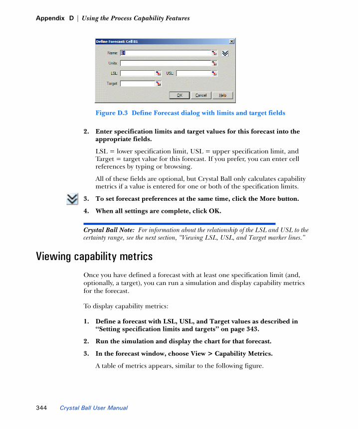
Appendix D | Using the Process Capability Features
Figure D.3 Define Forecast dialog with limits and target fields
2. Enter specification limits and target values for this forecast into the appropriate fields.
LSL = lower specification limit, USL = upper specification limit, and Target = target value for this forecast. If you prefer, you can enter cell references by typing or browsing.
All of these fields are optional, but Crystal Ball only calculates capability metrics if a value is entered for one or both of the specification limits.
3. To set forecast preferences at the same time, click the More button.
4. When all settings are complete, click OK.
Crystal Ball Note: For information about the relationship of the LSL and USL to the certainty range, see the next section, “Viewing LSL, USL, and Target marker lines.”
Viewing capability metrics Once you have defined a forecast with at least one specification limit (and, optionally, a target), you can run a simulation and display capability metrics for the forecast.
To display capability metrics:
1. Define a forecast with LSL, USL, and Target values as described in “Setting specification limits and targets” on page 343.
2. Run the simulation and display the chart for that forecast.
3. In the forecast window, choose View > Capability Metrics.
A table of metrics appears, similar to the following figure.
344 Crystal Ball User Manual

Viewing capability metrics1
Figure D.4 Capability Metrics view
For a description of each statistic, see “Capability metrics list” on page 353.
Viewing forecast charts and capability metrics togetherIt can be very helpful to view a forecast chart and its capability metrics side by side. This is now the default view when capability metrics are activated.
To do this manually:
1. Follow the instructions in the previous section to display capability metrics.
2. In the forecast window, choose View to open the View menu.
3. Choose Split View at the bottom of the menu.
4. Open the View menu again and choose Frequency.
The Frequency chart and capability metrics both appear, similar to the next figure.
Crystal Ball User Manual 345

Appendix D | Using the Process Capability Features
Figure D.5 Frequency chart and capability metrics in Split view
5. If you want, continue opening the menu and choosing charts or data.
The following figure shows a Frequency chart, a Cumulative Frequency chart, plus Statistics and Capability Metrics tables.
346 Crystal Ball User Manual

Viewing capability metrics1
Figure D.6 Frequency and Cumulative Frequency charts with capability metrics and statistics in Split view
You can click in any of the Split View panes and use the chart hot keys to modify them without using the View or Preferences menus. For a list, see Table 5.5 on page 129.
You can also resize the chart window and drag the horizontal and vertical pane splitters to resize each part of the Split View window.
Viewing LSL, USL, and Target marker linesBy default, after you add specification limits and a target to a forecast, markers for these values appear on the forecast chart. For an example, see Figure D.6.
Notice that the certainty range on the forecast chart changes to match the LSL and USL values. The certainty indicates the probability of falling within those specification limits. To show the certainty of different values, type them
Pane splitter
Crystal Ball User Manual 347

Appendix D | Using the Process Capability Features
into the Minimum and Maximum fields or click the certainty grabbers and drag them to a new position.
To add specification limit and target marker lines manually or to remove them:
1. Choose Preferences > Chart Preferences in a forecast chart window, or double-click the chart.
2. Click the Chart Type tab in the Chart Preferences dialog.
3. Scroll down to the bottom of the Marker Lines list.
Figure D.7 Showing and hiding LSL, USL, and target marker lines
4. Be sure LSL, USL, Target is checked if you want to display the specification limit and target marker lines on that forecast chart.
To hide the markers, uncheck LSL, USL, Target.
5. When all settings are complete, click OK.
Notice that you can display the mean and other marker lines in addition to the specification limit and target markers.
348 Crystal Ball User Manual

Extracting capability metrics1
Extracting capability metrics
Extracting capability metrics automaticallyYou can automatically extract capability metrics whenever a simulation runs. To do this:
1. In a forecast window, choose Preferences > Forecast and display the Auto Extract tab of the Forecast Preferences dialog.
Figure D.8 Choosing to Auto Extract Capability Metrics
2. Check Extract Forecast Statistics Automatically... and scroll down to the bottom of the data selection list.
3. Check Capability Metrics, enter a Starting Cell, and then click OK.
Now, when you run a simulation, capability metrics are written to the specified area of your worksheet, along with any other data you have requested.
For more information about the Auto Extract feature, see “Auto Extract preferences” on page 68. Be sure to choose an open area of your worksheet as the Starting Cell to avoid overwriting your model.
Crystal Ball User Manual 349

Appendix D | Using the Process Capability Features
Extracting capability metrics manuallyYou can also extract capability metrics manually after a simulation runs. To do this:
1. Choose Analyze > Extract Data to display the Extract Data Preferences dialog.
Figure D.9 Choosing to manually extract capability metrics
2. Check Capability Metrics at the bottom of the Select Data To Extract list.
3. Choose appropriate Forecasts and Assumptions settings and specify locations and other preferences on the Options tab. For more information, see “Extracting data” on page 190 or click the Help button in the Extract Data Preferences dialog.
4. Click OK to extract the data.
Capability metrics are written to the specified location, along with any other data you have requested. See Figure D.10 for an example.
350 Crystal Ball User Manual
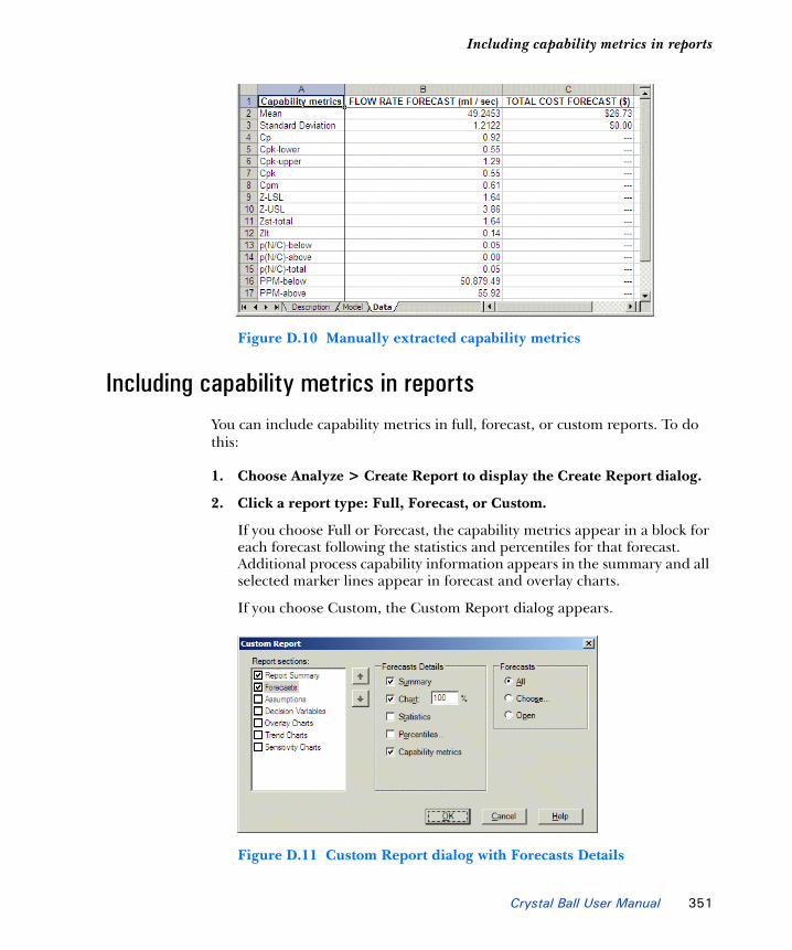
Including capability metrics in reports1
Figure D.10 Manually extracted capability metrics
Including capability metrics in reportsYou can include capability metrics in full, forecast, or custom reports. To do this:
1. Choose Analyze > Create Report to display the Create Report dialog.
2. Click a report type: Full, Forecast, or Custom.
If you choose Full or Forecast, the capability metrics appear in a block for each forecast following the statistics and percentiles for that forecast. Additional process capability information appears in the summary and all selected marker lines appear in forecast and overlay charts.
If you choose Custom, the Custom Report dialog appears.
Figure D.11 Custom Report dialog with Forecasts Details
Crystal Ball User Manual 351
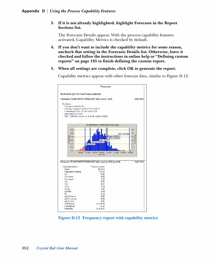
Appendix D | Using the Process Capability Features
3. If it is not already highlighted, highlight Forecasts in the Report Sections list.
The Forecasts Details appear. With the process capability features activated, Capability Metrics is checked by default.
4. If you don’t want to include the capability metrics for some reason, uncheck that setting in the Forecasts Details list. Otherwise, leave it checked and follow the instructions in online help or “Defining custom reports” on page 185 to finish defining the custom report.
5. When all settings are complete, click OK to generate the report.
Capability metrics appear with other forecast data, similar to Figure D.12.
Figure D.12 Frequency report with capability metrics
352 Crystal Ball User Manual

Capability metrics list1
Capability metrics listThe following table lists and defines the statistics shown in Capability Metrics view and indicates whether each statistic appears for long-term or short-term data. For a discussion of the equations used to calculate each of these statistics, see the online Crystal Ball Reference Manual.
Crystal Ball Note: Z scores are typically reported only for normal data. Crystal Ball always displays Z scores. It is up to the user to determine if the values are appropriate.
Table D.1 Capability statistics calculated by Crystal Ball
MetricLong-term
Short-term Description
Mean Mean of the forecast values
Standard deviation
Standard deviation of the forecast values
Cp Short-term capability index indicating what quality level the forecast output is potentially capable of producing. It is defined as the ratio of the specification width to the forecast width. If a Cp is equal to or greater than 1, then a short-term 3-sigma quality level is possible.
Pp Long-term capability index indicating what quality level the forecast output is potentially capable of producing. It is defined as the ratio of the specification width to the forecast width. If a Cp is equal to or greater than 1, then a long-term 3-sigma quality level is possible.
Cpk-lower
One-sided short-term capability index; for normally distributed forecasts, the ratio of the difference between the forecast mean and lower specification limit over three times the forecast short-term standard deviation; often used to calculate process capability indices with only a lower specification limit.
Ppk-lower
One-sided long-term capability index; for normally distributed forecasts, the ratio of the difference between the forecast mean and lower specification limit over three times the forecast long-term standard deviation; often used to calculate process capability indices with only a lower specification limit.
Cpk-upper
One-sided short-term capability index; for normally distributed forecasts, the ratio of the difference between the forecast mean and upper specification limit over three times the forecast short-term standard deviation; often used to calculate process capability indices with only an upper specification limit.
Crystal Ball User Manual 353
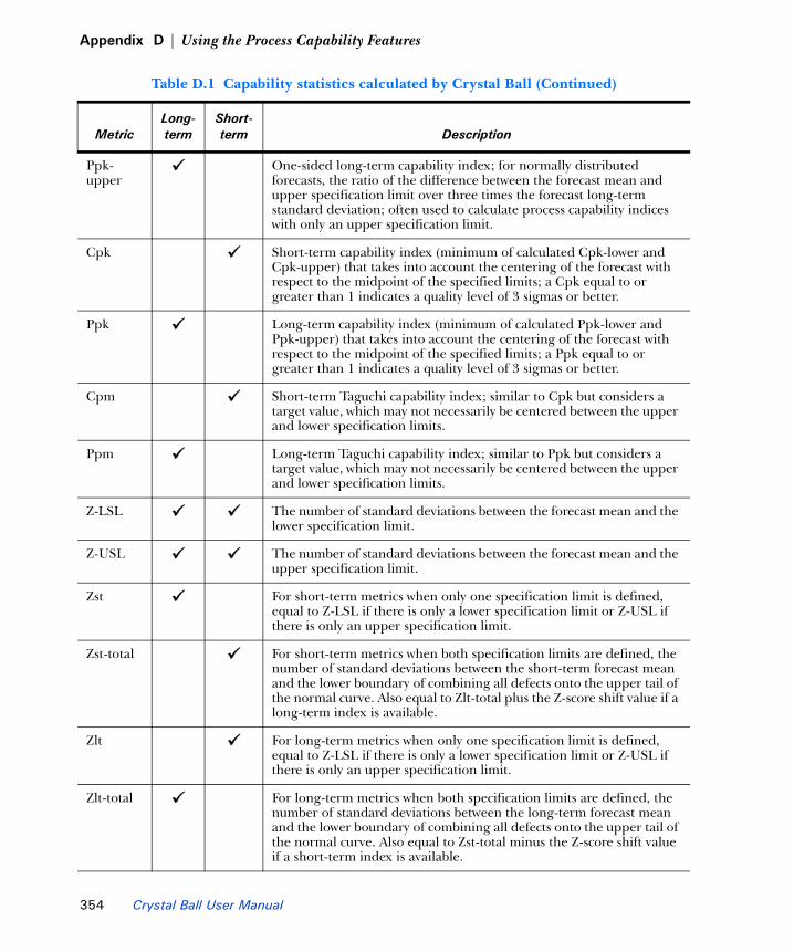
Appendix D | Using the Process Capability Features
Ppk-upper
One-sided long-term capability index; for normally distributed forecasts, the ratio of the difference between the forecast mean and upper specification limit over three times the forecast long-term standard deviation; often used to calculate process capability indices with only an upper specification limit.
Cpk Short-term capability index (minimum of calculated Cpk-lower and Cpk-upper) that takes into account the centering of the forecast with respect to the midpoint of the specified limits; a Cpk equal to or greater than 1 indicates a quality level of 3 sigmas or better.
Ppk Long-term capability index (minimum of calculated Ppk-lower and Ppk-upper) that takes into account the centering of the forecast with respect to the midpoint of the specified limits; a Ppk equal to or greater than 1 indicates a quality level of 3 sigmas or better.
Cpm Short-term Taguchi capability index; similar to Cpk but considers a target value, which may not necessarily be centered between the upper and lower specification limits.
Ppm Long-term Taguchi capability index; similar to Ppk but considers a target value, which may not necessarily be centered between the upper and lower specification limits.
Z-LSL The number of standard deviations between the forecast mean and the lower specification limit.
Z-USL The number of standard deviations between the forecast mean and the upper specification limit.
Zst For short-term metrics when only one specification limit is defined, equal to Z-LSL if there is only a lower specification limit or Z-USL if there is only an upper specification limit.
Zst-total For short-term metrics when both specification limits are defined, the number of standard deviations between the short-term forecast mean and the lower boundary of combining all defects onto the upper tail of the normal curve. Also equal to Zlt-total plus the Z-score shift value if a long-term index is available.
Zlt For long-term metrics when only one specification limit is defined, equal to Z-LSL if there is only a lower specification limit or Z-USL if there is only an upper specification limit.
Zlt-total For long-term metrics when both specification limits are defined, the number of standard deviations between the long-term forecast mean and the lower boundary of combining all defects onto the upper tail of the normal curve. Also equal to Zst-total minus the Z-score shift value if a short-term index is available.
Table D.1 Capability statistics calculated by Crystal Ball (Continued)
MetricLong-term
Short-term Description
354 Crystal Ball User Manual

Capability metrics list1
p(N/C)-below
Probability of a defect below the lower specification limit; DPUBELOW
p(N/C)-above
Probability of a defect above the upper specification limit; DPUABOVE
p(N/C)-total
Probability of a defect outside the lower and upper specification limits; DPUTOTAL
PPM-below
Defects below the lower specification limit, per million units
PPM-above
Defects above the upper specification limit, per million units
PPM-total
Defects outside both specification limits, per million units
LSL Lower specification limit, the lowest acceptable value of a forecast involved in process capability, or quality, analysis.
USL Upper specification limit, the highest acceptable value of a forecast involved in process capability analysis.
Target The ideal target value of a forecast involved in process capability analysis.
Z-score shift
An optional shift value to use when calculating long-term capability metrics. The default, set in the Capability Options dialog, is 1.5.
Table D.1 Capability statistics calculated by Crystal Ball (Continued)
MetricLong-term
Short-term Description
Crystal Ball User Manual 355

Appendix D | Using the Process Capability Features
356 Crystal Ball User Manual

Crystal Ball User Manual 357
Bibliography
In this bibliography• Bootstrap• Monte Carlo simulation• Probability theory and statistics• Random variate generation methods• Specific distributions• Extreme value distribution• Lognormal distribution• Weibull distribution• Tornado charts and sensitivity analysis• Two-Dimensional simulation• Weibull distribution• Uncertainty analysis

Bibliography
Bootstrap
Efron, Bradley, and Robert J. Tibshirani. “An Introduction to the Bootstrap,” Monographs on Statistics and Applied Probability, vol. 57. New York: Chapman and Hall, 1993.
Mooney, C. Z., and R.D. Duval. “Bootstrapping: A Nonparametric Approach to Statistical Inference,” Sage University Paper Series on Quantitative Applications in the Social Sciences, series no. 07-095. Newbury Park, CA: Sage, 1993.
Monte Carlo simulation
Burmaster, D.E., and P.D. Anderson, “Principles of Good Practice for the Use of Monte Carlo Techniques in Human Health and Ecological Risk Assessments,” Risk Analysis 14(4): 477-481 (1994).
Hammersley, J.M., and D.C. Handscomb. Monte Carlo Methods. New York: Chapman and Hall, 1965.
Kalos, Malvin H., and Paula A. Whitlock. Monte Carlo Methods. New York: John Wiley & Sons, 1986.
Morgan, Byron J.T. Elements of Simulation. Portland, ME: Chapman and Hall, 1984.
Rubinstein, Reuven Y. Simulation and the Monte Carlo Method. New York: John Wiley & Sons, 1981.
Thommes, M.C. Proper Spreadsheet Design. Boston: Boyd and Fraser Publishing Co., 1992.
Thompson, K.M., D.E. Burmaster, and E.A.C. Crouch. “Monte Carlo Techniques for Quantitative Uncertainty Analysis in Public Health Risk Assessments,” Risk Analysis 12(1): 53-63 (1992).
Yakowitz, Sidney J. Computational Probability and Simulation. Reading, MA: Addison-Wesley Publishing Co., 1977.
Probability theory and statistics
Alder, Henry L., and Edward B. Roessler. Introduction to Probability and Statistics, 6th Ed. San Francisco: W.H. Freeman & Co, 1977.
358 Crystal Ball User Manual

1
Biswas, Suddhendu. Topics in Statistical Methodology. New York: John Wiley & Sons, Inc., 1991.
Fraser, D.A.S. Probability and Statistics: Theory and Applications. North Scituate, MA: Duxbury Press, 1976.
Johnson, Norman L., and Samuel Kotz. Distributions in Statistics: Continuous Multivariate Distributions. New York: John Wiley & Sons, Inc., 1972.
Kapur, K.C., and L.R. Lamberson. Reliability in Engineering Design. New York: John Wiley & Sons, 1977.
Larson, Harold J. Introduction to Probability Theory and Statistical Inference, 2nd Ed. New York: John Wiley & Sons, 1974.
Logothetis, N., and V. Rothschild. Probability Distributions. New York: John Wiley & Sons, Inc., 1986.
Spurr, William, and Charles P. Bonini. Statistical Analysis for Business Decisions. Homewood, IL: Richard D. Irwin, Inc., 1973.
Wadsworth, George P., and Joseph G. Bryan. Introduction to Probability and Random Variables. New York: McGraw-Hill Book Co., 1960.
Winkler, Robert L., and William L. Hays. Statistics: Probability, Inference, and Decision. New York: Holt, Rinehart, and Winston, 1975.
Random variate generation methods
Devroye, Luc. Non-Uniform Random Variate Generation. New York: Springer-Verlag, 1986.
Iman, Ronald L., and W.J. Conover. “A Distribution-Free Approach to Inducing Rank Correlation Among Input Variables,” Communications in Statistics B11(3):1982.
Iman, Ronald L., and J.M. Davenport. “Rank Correlation Plots for Use With Correlated Input Variables,” Communications in Statistics B11(3): (1982).
Iman, Ronald L., and J.M. Davenport. Latin Hypercube Sampling (A Program User’s Guide). Technical Report SAND79-1473, Sandia National Laboratories, 1980.
Kennedy, William J., Jr., and James E. Gentle. Statistical Computing. New York: Marcel Dekker, Inc., 1980.
Crystal Ball User Manual 359

Bibliography
Knuth, Donald E. The Art of Computer Programming, Vols I-III. Reading, MA: Addison-Wesley Publishing Co., 1969.
Newman, Thomas G., and Patrick L. Odell. The Generation of Random Variates. New York: Hafner Publishing Co., 1971.
Press, William H., et al. Numerical Recipes in C, 2nd Ed. Cambridge, England: Cambridge University Press, 1993.
Odeh, R.E., and J.O. Evans. “Percentage Points of the Normal Distribution,” Applied Statistics. London: Royal Statistical Society, 1974.
Sedgewich, Robert. Algorithms. Reading, MA: Addison Wesley Publishing Co., 1983.
Specific distributions
Extreme value distributionCastillo, Enrique. Extreme Value Theory in Engineering. London: Academic Press, 1988.
Lognormal distributionAitchison, J., and J.A. Brown. The Lognormal Distribution. New York: Cambridge University Press, 1973.
Weibull distributionKing, James R. Probability Charts for Decision Making, Rev. Ed. New York: Industrial Press, Inc., 1981.
Henley, Ernest J., and Hiromitsu Kumamoto. Reliability Engineering and Risk Assessment. Englewood Cliffs, NJ: Prentice Hall, Inc., 1981.
Tornado charts and sensitivity analysis
Clemen, Robert T. Making Hard Decisions: An Introduction to Decision Analysis, 2nd Ed. Belmont, CA: Duxbury Press, 1997.
360 Crystal Ball User Manual

1
Morgan, M. Granger, and Max Henrion; with a chapter by Mitchell Small. Uncertainty: A Guide to Dealing with Uncertainty in Quantitative Risk and Policy Analysis. New York: Cambridge University Press, 1990.
Two-Dimensional simulation
Burmaster, David E., and Andrew M. Wilson. “An Introduction to Second-Order Random Variables in Human Health Risk Assessments,” Human and Ecological Risk Assessment 2(4): 892-919 (1996).
Frey, H. Christopher, and David S. Rhodes. “Characterizing, Simulating, and Analyzing Variability and Uncertainty: An Illustration of Methods Using an Air Toxics Emissions Example,” Human and Ecological Risk Assessment 2(4): 762-797 (1996).
Hoffman, F.O., and J.S. Hammonds. “Propagation of Uncertainty in Risk Assessments: The Need to Distinguish Between Uncertainty Due to Lack of Knowledge and Uncertainty Due to Variability” Risk Analysis 14(5): 707-712 (1994).
Rai, S. N., D. Drewski, and S. Bartlett. “A General Framework for the Analysis of Uncertainty and Variability in Risk Assessment,” Human and Ecological Risk Assessment 2(4): 972-989 (1996).
Uncertainty analysis
Morgan, M. Granger, and Max Henrion; with a chapter by Mitchell Small. Uncertainty: A Guide to Dealing with Uncertainty in Quantitative Risk and Policy Analysis. New York: Cambridge University Press, 1990.
Hoffman, F.O., and J.S. Hammonds. “Propagation of Uncertainty in Risk Assessments: The Need to Distinguish Between Uncertainty Due to Lack of Knowledge and Uncertainty Due to Variability” Risk Analysis 14(5): 707-712 (1994).
International Atomic Energy Agency, “Evaluating the Reliability of Predictions Made Using Environmental Transfer Models,” IAEA Safety Series No. 100:1-106. STI/PUB/835. Vienna, Austria, 1989.
Kelton, W. David, and Averill M. Law. Simulation Modeling & Analysis, 3rd Ed. New York: McGraw-Hill, Inc. 2000.
Crystal Ball User Manual 361

Bibliography
362 Crystal Ball User Manual

Crystal Ball User Manual 363
Glossary
In this glossaryA compilation of terms specific to Crystal Ball as well as statistical terms used in this manual.
Additional definitions and details are included in the Crystal Ball Reference Manual, accessed online by choosing Start > Programs > Crystal Ball 7 > Documentation.

Glossary
algorithmA rule that specifies how to solve a particular problem.
assumptionAn estimated value or input to a spreadsheet model.
assumption cellA value cell in a spreadsheet model that has been defined as a probability distribution.
base caseThe value in a Crystal Ball assumption, decision variable, or forecast cell at the start of a simulation.
CDFCumulative distribution function that represents the probability that a variable will fall at or below a given value.
certainty bandsIn a trend chart, a graphic depiction of a particular certainty range for each forecast.
certainty levelThe percentage of values in the certainty range compared to the number of values in the entire range.
certainty rangeThe linear distance for the set of values between the certainty grabbers on the forecast chart.
coefficient of variability also coefficient of variance or coefficient of variationA measure of relative variation that relates the standard deviation to the mean. Results can be represented in percentages for comparison purposes.
continuous probability distributionA probability distribution that describes a set of uninterrupted values over a range. In contrast to the discrete distribution, the continuous distribution assumes there is an infinite number of possible values.
correlationIn Crystal Ball, a dependency that exists between assumption cells.
364 Crystal Ball User Manual

1
correlation coefficientA number between -1 and 1 that specifies mathematically the degree of positive or negative correlation between assumption cells. A correlation of 1 indicates a perfect positive correlation, minus 1 indicates a perfect negative correlation, and 0 indicates there is no correlation.
cumulative frequency distributionA chart that shows the number or proportion (or percentage) of values less than or equal to a given amount.
decision variable cellCells that contain the values or variables that are within your control to change. The decision variable cells must contain simple numeric values, not formulas or text.
decision variableA Crystal Ball variable in your model that you can control.
deterministic modelAnother name for a spreadsheet model which yields single-valued results.
discrete probability distributionA probability distribution that describes distinct values, usually integers, with no intermediate values. In contrast, the continuous distribution assumes there is an infinite number of possible values.
display rangeThe linear distance for the set of values displayed on the forecast chart.
dominantA relationship between distributions in which one distribution’s values for all percentile levels are higher than another’s. (see also subordinate)
entire rangeThe linear distance from the minimum forecast value to the maximum forecast value.
forecastA statistical summary of the assumptions in a spreadsheet model, output graphically or numerically.
Crystal Ball User Manual 365

Glossary
forecast cellCells that contain formulas that refer to one or more assumption and decision variable cells and combine the values in the assumption, decision, and other cells to calculate a result.
forecast definitionThe forecast name and parameters assigned to a cell in a Crystal Ball dialog.
forecast filteringA process by which Crystal Ball discards forecast values outside or inside a specified range.
forecast formulaA formula that has been defined as a forecast cell.
forecast value also trialA value calculated by the forecast formula during an iteration. These values are kept in a list for each forecast, and are summarized graphically in the forecast chart and numerically in the descriptive statistics.
formula cellA cell that contains a mathematical formula.
frequency also frequency countThe number of times a value recurs in a group interval.
frequency distributionA chart that graphically summarizes a list of values by sub-dividing them into groups and displaying their frequency counts.
goodness-of-fitA set of mathematical tests performed to find the best fit between a standard probability distribution and a data set.
grabber also certainty grabber or truncation grabberA control that lets you use the mouse to change values and settings.
group intervalA subrange of a distribution that allows similar values to be grouped together and given a frequency count.
366 Crystal Ball User Manual
1
iteration also trialA three-step process in which Crystal Ball generates random numbers for assumption cells, recalculates the spreadsheet model or models, and displays the results in a forecast chart.
kurtosisThe measure of the degree of peakedness of a curve. The higher the kurtosis, the closer the points of the curve lie to the mode of the curve. A normal distribution curve has a kurtosis of 3.
Latin hypercube samplingIn Crystal Ball, a sampling method that divides an assumption’s probability distribution into intervals of equal probability. The number of intervals corresponds to the Minimum Sample Size option available in the Run Preferences dialog. A random number is then generated for each interval. Compared with conventional Monte Carlo sampling, Latin hypercube sampling is more precise because the entire range of the distribution is sampled in a more even, consistent manner. The increased accuracy of this method comes at the expense of added memory requirements to hold the full Latin hypercube sample for each assumption. (See “Sampling preferences” on page 83.)
meanThe familiar arithmetic average of a set of numerical observations: the sum of the observations divided by the number of observations.
mean standard errorThe Standard Deviation of the distribution of possible sample means. This statistic gives one indication of how accurate the simulation is.
medianThe value midway (in terms of order) between the smallest possible value and the largest possible value.
modeThat value which, if it exists, occurs most often in a data set.
model sensitivityThe overall effect that a change in an assumption cell produces in a forecast cell. This effect is solely determined by the formulas in the spreadsheet model.
Crystal Ball User Manual 367

Glossary
Monte Carlo simulationA system which uses random numbers to measure the effects of uncertainty in a spreadsheet model.
outliers also outlying valuesValues generated during a simulation on the extreme end of a distribution and are excluded from the display range.
PDFProbability density function that represents the probability that an infinitely small variable interval will fall at a given value.
probabilistic modelA system whose output is a distribution of possible values. In Crystal Ball, this system includes a spreadsheet model (containing mathematical relationships), probability distributions, and a mechanism for determining the combined effect of the probability distributions on the model’s output (Monte Carlo simulation).
probability(Classical Theory) The likelihood of an event.
probability distribution also distributionA set of all possible events and their associated probabilities.
random numberA mathematically selected value which is generated (by a formula or selected from a table) to conform to a probability distribution.
random number generatorA method implemented in a computer program that is capable of producing a series of independent, random numbers.
rangeThe difference between the largest and smallest values in a data set.
rank correlation also Spearman’s rank correlationA method whereby assumption values are replaced with their ranking from lowest value to highest value using the integers 1 to N prior to computing the correlation coefficient. This method allows the distribution types to be ignored when correlating assumptions.
368 Crystal Ball User Manual

1
relative probability also relative frequencyA value, not necessarily between 0 and 1, that indicates probability when used in a proportion.
reverse cumulative frequency distributionA chart that shows the number or proportion (or percentage) of values greater than or equal to a given amount.
riskThe uncertainty or variability in the outcome of some event or decision.
seed valueThe first number in a sequence of random numbers. A given seed value produces the same sequence of random numbers every time you run a simulation.
sensitivityThe amount of uncertainty in a forecast cell that is a result of both the uncertainty (probability distribution) and model sensitivity of an assumption cell.
sensitivity analysisThe computation of a forecast cell’s sensitivity with respect to the assumption cells.
skewedAn asymmetrical distribution.
skewed, negativelyA distribution in which most of the values occur at the upper end of the range.
skewed, positivelyA distribution in which most of the values occur at the lower end of the range.
skewnessThe amount a curve differs from a normal, symmetrical distribution. The greater the degree of skewness, the more points of the curve lie to either side of the peak of the curve. A normal distribution curve, having no skewness, is symmetrical. Skewness is computed by finding the third moment about the mean and dividing by the cube of the standard deviation.
Crystal Ball User Manual 369

Glossary
spreadsheet modelAny spreadsheet that represents an actual or hypothetical system or set of relationships.
standard deviationThe square root of the variance for a distribution. A measurement of the variability of a distribution, i.e., the dispersion of values around the mean. (See formulas in “Standard deviation” in the “Statistical Definitions” chapter of the online Crystal Ball Reference Manual.)
subordinateA relationship between distributions in which one distribution’s values for all percentile levels are lower than another’s. (see also dominant)
trial also iterationA three-step process in which Crystal Ball generates random numbers for assumption cells, recalculates the spreadsheet model or models, and displays the results in a forecast chart.
trial as used to describe a parameter in certain probability distributionsThe number of times a given experiment is repeated.
value cellA cell that contains a simple numeric value.
variableA quantity that can assume any one of a set of values and is usually referenced by a formula.
varianceThe square of the standard deviation; i.e., the average of the squares of the deviations of a number of observations from their mean value.
Variance can also be defined as a measure of the dispersion, or spread, of a set of values about a mean. When values are close to the mean, the variance is small. When values are widely scattered about the mean, the variance is large. (See formulas in “Variance” in the “Statistical Definitions” chapter of the online Crystal Ball Reference Manual.)
virtual memoryMemory which uses your hard drive space to store information after you run out of random access memory. Virtual memory supplements your random access memory.
370 Crystal Ball User Manual
1
workbookAn Excel file composed of at least one worksheet.
worksheetAn Excel file in which you work and store your data. A worksheet is part of a workbook.
Crystal Ball User Manual 371

Glossary
372 Crystal Ball User Manual
Index
In this indexA comprehensive index designed to give you quick access to the information in this manual.
Crystal Ball User Manual 373

Index
Aabsolute cell references 24, 25alternate parameters 25, 255analyzing simulation results, guidelines 104Anderson-Darling test 29, 121Apply To 139applying settings 139assumption
preferences 38assumption cells
defined 18assumption parameters
alternate 25Assumption Preferences dialog 39assumptions
correlated 33defining 19entering 19freezing 88selecting and reviewing 72
Auto Extract preferences 68
BBatch Fit
example 199tool 199
beta distributiondefined 255
bibliography 360binomial distribution
defined 281Bootstrap
example 221tool 219
bootstrap methods 219
Ccapability metrics 340categories
creating distribution 50deleting distribution 51rearranging distribution 51sharing distribution 52, 53, 54, 55viewing and editing distribution properties
51categories, managing distribution 49Category pane,Distribution Gallery 44caveats, tornado and spider charts 218cell preferences 74
cell references 24absolute 25dynamic and static 24relative 25
certainty levelsforecast chart 107trend charts 162
certainty, defined 12chart preferences 128chart preferences hot keys 129charts
closing 142copying 141customizing 128deleting 143displaying 140managing 140overlay with Two-dimensional Simulation
241pasting 141preferences 128printing 142sensitivity 165spider 213tornado 211trend, with Two-dimensional Simulation 241
chi-square distribution 261chi-square test 29, 122chi-squared distribution 259Choose Assumptions dialog 35Choose Forecasts dialog 192closing charts 142comparing distributions 313comparison chart
overview 30consulting referral service 6continuing a simulation 90continuous
distributions 249Control Panel, Crystal Ball 93Control Panel, hiding 93Control Panel, showing after reset 93control, precision
defining with forecast 59displayed percentiles 118displayed statistics 118increasing accuracy 318
conventions, manual 4copying charts 141
374 Crystal Ball User Manual

1
copying distributions 46correlated assumptions, practical limit 323Correlation chart 38Correlation Matrix
example 207tool 206
correlationsaccuracy 318defined 206specifying 33
creating distribution categories 50creating distributions 45Crystal Ball
Monte Carlo simulation 78system requirements 1
Crystal Ball Control Panel 93custom distribution 294
important notes 311customizing charts 128
Ddata
editing 69grouped 302
data, entering custom 306Decision Table
example 227tool 226
decision variable cellsdefined 18
decision variablesdefining 58
defaults, setting 139Define Correlation dialog 35Define Forecast dialog, expanded 61defining assumptions 19deleting charts 143deleting distribution categories 51deleting distributions 48Description pane,Distribution Gallery 45dialogs
Choose Forecasts 192Select 73
discretedistributions 249ranges 302
discrete uniform distribution 283display range preferences 112displaying charts 140
distributionpreferences 38
distribution categories 49creating 50deleting 51rearranging 51sharing 52, 53, 54, 55
distribution category propertiesediting and viewing 51
distribution fittingoverlay charts 152, 153overview 27
Distribution GalleryCategory pane 44Description pane 45displaying 42Distribution pane 44managing categories 49managing distributions 45menubar and buttons 43using 41window 42
Distribution Gallery tasks 41Distribution pane,Distribution Gallery 44distributions
chi-squared 259copying 46creating 45deleting 48discrete or continuous 249Erlang 259managing 45modifying 47, 48pasting 46truncating 312
distributions as Excel functions 315distributions, parameters 255distributions, probability 12dynamic cell referencing 24
Eediting distribution category properties 51emailing distribution categories 54entering custom data 306Erlang distribution 259erlang distribution 261examples
Batch Fit 199Bootstrap 221
Crystal Ball User Manual 375
Index
Correlation Matrix 207Decision Table 227Scenario Analysis 231Tornado Chart 214Two-dimensional Simulation 237
Excel chartspasting to 141
Excel functions and distributions 315expanded Define Forecast dialog 61exponential distribution
defined 257extenders, see tools 198extract data 190extreme distributions
defined 265, 267
FFilter preferences 66fitting distributions
overview 27forecast cells
defined 18forecast charts
distribution types 115format 113groups 127
forecast charts, analyzing 104Forecast Preference dialog 61forecast preferences 61Forecast Preferences dialog
Auto Extract tab 68Filter tab 66Forecast Window tab 62Precision tab 64
Forecast Window preferences 62forecasts
defining 59fitting distributions 27percentiles view 118selecting and reviewing 72statistics view 118understanding 106
forecasts, defined 12formulas in parameters 25freezing assumptions 88
Ggamma distribution
defined 259
geometric distributiondefined 285
global macros 102goodness-of-fit tests 27grouped data 302groups 127guidelines
analyzing simulation results 104
H-Khelp, online 5hot keys for charts 129how this manual is organized 2hypergeometric distribution
defined 286insufficient memory warning 87Kolmogorov-Smirnov test 29, 122
LLatin hypercube sampling
accuracy 318logistic distribution
defined 262lognormal distribution
defined 263parameter sets 265
Mmacros
global 102user-defined 99
managing categoriesDistribution Gallery 49
managing charts 140managing distirbutions
Distribution Gallery 45manual conventions 4maximum extreme distribution 265memory
warning of insufficient 87methods, bootstrap 219minimum extreme distribution 267model sensitivity 165modifying distributions 47, 48monotonic relationships 212Monte Carlo simulation
benefits 13defined 11in Crystal Ball 78
376 Crystal Ball User Manual

1
Nnegative binomial distribution 289New Category dialog 50next distribution/prev. distribution 30normal distribution
defined 268
Oonline help 5outliers 107outlying values 107overlay chart, with Two-dimensional Simulation
241overlay charts
customizing 151distribution fitting 152, 153overview 146
Overlay Example 149
Pparameters
alternate 25formulas 25range names 25
Parameters menu 255parameters, alternate 255Pareto distribution
defined 270pasting charts 141pasting distributions 46percentiles
reversing 88view 118
Poisson distributiondefined 291
precision controldefining with forecast 59displayed percentiles 118displayed statistics 118increasing accuracy 318
Precision preferences 64Preferences menu
distributions 38preferences, chart 128printing charts 142probability 246probability distributions 12
beta 255binomial 281
chi-square 261comparing 313custom 294discrete uniform 283erlang 261exponential 257extreme, maximum 265extreme, minimum 267gamma 259geometric 285hypergeometric 286logistic 262lognormal 263negative binomial 289normal 268Pareto 270Poisson 291selecting 250Student’s t 272triangular 274uniform 276yes-no 293
process capability features 340properties
distribution category 51publishing distribution categories 52
Qquality features 340
Rrange names in parameters 25ranking methods 32rearranging distribution categories 51references 360
absolute cell 25dynamic and static 24relative cell 25
references, cell 24referrals, consulting 6relative cell references 24relative cell referencing 25relative probability 296reports
overview 182requirements 1resetting a simulation 90restoring simulation results 98reversed percentiles 88
Crystal Ball User Manual 377

Index
run preferences 80running a simulation 90
Ssaving and restoring simulation results 97saving simulation results 97Scenario Analysis
example 231tool 231
screen capture notes 5second-order variables 243Select dialog 73selecting some data 73sending distribution categories 54sensitivity analysis
accuracy 318calculation 170
sensitivity chartscreating 167customizing 172overview 165
setting defaults 139setting forecast preferences 61sharing distribution categories 52, 53, 54, 55simulation results, restoring 98simulation results, saving 97simulation results, saving and restoring 97simulation results, using 99simulations
accuracy 318speed 321
Single Step 93Six Sigma features 340skewness
in lognormal distribution 263spider chart 213static cell referencing 24statistics view 118stopping a simulation 90Student’s t distribution 272Subscribe To A Category dialog 53subscribing to distribution categories 53support, technical 5system requirements 1
Ttables, Two-dimensional Simulation results 240tasks
Distribution Gallery 41
technical support 5Test Data example 32tools
Batch Fit 199Bootstrap 219Correlation Matrix 206Decision Table 226Scenario Analysis 231Tornado Chart 211Two-dimensional Simulation 236
Tornado Chartdescription 211example 214tool 211uses 211
training service 5trend chart, with Two-dimensional Simulation
241trend charts
certainty levels 162creating 155customizing 157overview 154value axis 163
triangular distributionoverview 274
truncating distributions 312tutorials
Test Data 32Two-dimensional Simulation
example 237tool 236
Uuncertainty 236uniform distribution
defined 276unpublishing distribution categories 55user manual conventions 4user-defined macros 99using simulation results 99
Vvalue axis settings 163variability
vs. uncertainty 236variables, decision
defining 58variables, second-order 243
378 Crystal Ball User Manual

1
viewing distribution category properties 51virtual memory 322
WWeibull distribution
example 33who should use this program 1
Yyes-no distribution 293
Crystal Ball User Manual 379

Crystal Ball User Manual 379
Credits
Crystal Ball User Manual
Written and edited by Barbara Gentry, Eric Wainwright, and David Blankinship.
Portions based on material written and edited by Carol Werckman, Terry Hardy, Cameron Harris, and Roy Sargent.
Illustrations and screen captures by Barbara Gentry using Jasc, Inc. Paint Shop Pro.
Typeset using NewBskvll BT and Univers fonts.
