1

Finite element modelling of small-scale hot deformation testing

CUED/C-MATS/TR264

December 2019

P. Jędrasiak, H.R. Shercliff

ISSN: 0309-6505

Department of Engineering University of Cambridge

Trumpington St Cambridge

CB2 1PZ, UK

2

Abstract This report presents a finite element model of small-scale hot compression testing, using a dilatometer in loading mode. The main goal is to correct the true stress-strain hot constitutive response as a function of temperature and strain-rate, accounting for friction between the platens and workpiece, and the temperature gradient along the sample. The model also provides quantitative prediction of the spatial and temporal variation in strain-rate and strain throughout the sample, which is needed to correlate the local deformation conditions with the microstructure/texture evolution.

The study is based on a detailed series of 144 hot compression tests of a zirconium alloy (Zr-2.5Nb), at strain-rates ranging from 10-2.5 to 10s-1, and temperatures between 650°C to 850°C, with duplicate tests at all nominal test conditions. The Zr alloy is an important wrought material in its own right, in the context of the nuclear industry, but also serves as an analogue for other high temperature alloys (notably titanium) which show a dual α-β phase microstructure in a comparable temperature range.

The finite element model of the dilatometer test demonstrated that deformation conditions in the sample were substantially non-uniform, compared to the nominal temperature and strain-rate. The heating and cooling capabilities of the dilatometer were able to maintain reasonably isothermal conditions at the centre of the sample at moderate strain-rates, but not at rates of 1s-1 or above; but in all cases the temperature gradient and friction led to inhomogeneous deformation and barrelling. To account for these factors, a novel method is presented for correcting the true stress-strain (i.e. from the notional response allowing only for the idealised change in sample length and area), to give a true constitutive response over the full range of temperatures, strain-rates and strain.

The analysis in this report includes a number of alternative approaches to capturing the material constitutive data in equations or look-up tables, and also detailed sensitivity analysis on the FE-predicted spatial histories of deformation, as a function of the assumed material model and friction coefficient, for different test temperatures, temperature gradients and strain-rates. The FE-corrected constitutive data have been applied for a number of applications, for example, the generation of “processing maps” for Zr-2.5Nb, demonstrating the importance of allowing for inhomogeneity and meaningful statistical fitting of the data; this work is presented in more detail elsewhere [1].

Acknowledgements This research was funded by LightForm, a UK Engineering and Physical Sciences Research Council (EPSRC) programme grant (EP/R001715/1). The authors wish to acknowledge the contribution of our LightForm colleagues: Dr Graham McShane at the University of Cambridge, and Dr. Chris Daniel and Prof. João Quinta da Fonseca at the University of Manchester, for provision of the test data and for technical discussions; we also thank Chris Peyton, who conducted the experimental work on the dilatometer.

3

1. Introduction

1.1 Zr-2.5Nb processing and microstructure

Zr-2.5Nb is the most important commercial zirconium alloy alongside zircalloys (based on Zr-Sn), used in the cladding and pressurised tubing of nuclear reactors. The addition of Nb improves the corrosion resistance and hardness. Owing to their higher strength, better creep resistance, and limited hydrogen absorption in comparison with Zr-Sn alloys, the Zr-Nb alloys allow for thinner-walled pressure tubes, improving the neutron economy of the reactor [2].

Zr-2.5Nb is a two-phase material, with hexagonal close-packed (HCP) α grains and body-centred cubic (BCC) β phase. In Zr-Nb alloys with 0.6% < wt% Nb < 20%, slow cooling through the upper α/β phase field (927 to 602°C) leads to the formation of equilibrium αZr phase and βZr; further cooling leads to a eutectoid breakdown of the βZr into αZr and Nb-rich βNb. The specific thermo-mechanical processing route for Zr alloys is chosen to control the development of the α-β microstructure and the crystallographic texture. For example, in the present study the Zr-2.5Nb alloy was specifically produced to obtain a small prior-β grain size, through forging a 27 inch diameter ingot to a 5 inch thick slab, and hot rolling to 3 inches thick. The initial forged microstructure was air-cooled from just above the β-transus (measured to be 890°C), resulting in a microstructure of Widmanstätten packets of α-laths, separated by fine filaments of retained metastable βZr [1].

A better understanding of the effect of processing parameters on two-phase microstructure and texture evolution during high temperature deformation is required, to minimise process development costs and for optimisation of the processing route. Conventionally this is achieved by lab-scale compression (or torsion) testing over a matrix of (nominally constant) temperature and strain-rate conditions. However it is difficult to achieve homogeneity of temperature and strain, due to friction at the interface between workpiece and platens, and a combination of imposed sample heating, heat generation by hot working, and heat losses to the platens and surrounding atmosphere. Hence “modelling the test” is necessary to predict the local deformation conditions. This however requires constitutive data for the hot deformation response – which is itself one of the intended outputs of the experiments, but only obtained as an average response of a sample undergoing non-uniform deformation.

This report demonstrates a method for modelling small-scale hot compression tests using a dilatometer in loading mode, allowing for the inhomogeneity in the workpiece deformation. The load-displacement data are used to give a first estimate of a ‘notional’ true stress-strain response as input to the finite element analysis. This proves to be sufficient to predict the correction needed to the data to give a true stress-strain response for the alloy in a single iteration, while also predicting the spatial variation in conditions over the sample.

1.2 Process and constitutive modelling

Process modelling

Modelling of manufacturing processes has become routine for most technologies over the last 50 years, in particular using the finite element method. Process models primarily offer value in reducing the need for empirical tests, reducing the cost and development time for: component design-for-manufacture, improved shape and property control, reduction of defects, tool and die design, improving productivity, and developing new alloys. Modelling of manufacturing steps is also often integrated with software to analyse subsequent product performance [3] [4].

Modelling applications span the entire spectrum of industrial alloys in all deformation processing – forging, rolling, drawing, extrusion, solid-state joining, sheet forming, hydroforming, and creep forming – often integrated with heat treatment conducted immediately after forming (e.g. annealing, quenching). Modelling also plays a role in the lab, for analysis of “standard tests”, used for determining constitutive

4

behaviour, or for scientific studies of microstructure and property evolution under controlled conditions [3] [4].

Process modelling example: forging

Laboratory hot compression testing is a common idealisation for modelling forging processes. Models contribute to optimisation of die design and process conditions in net-shape and multi-step forging, and prediction of final grain structure, texture, mechanical properties, and residual stress. Hot forging simulations for large deformations may use a flow-type formulation with an Eulerian framework, where the metal behaves as a high viscosity fluid, and elastic behaviour is ignored. More generally, elastic–plastic formulations are employed in a Lagrangian framework. Most forging simulations include temperature evolution, capturing heating due to plastic dissipation and heat losses to the tooling and surrounding air, requiring either a fully coupled thermomechanical model, or separate thermal and deformation models [5]. Key aspects of forging models are the effects of the tool-workpiece interface (friction, war and heat transfer) on the deformation and temperature fields, and the loading at the interface. Amongst deformation processes, the complexity of forging is high, due to the changing 3D part geometry and temperature distribution, and discontinuous, frictional tool-workpiece contact. This has driven much of the development of finite element techniques for process modelling, to realise efficient computation run-times through re-meshing, adaptive meshing, parallel computation, and multigrid algorithms, while managing convergence problems [5].

Constitutive modelling

Constitutive data, relating the states of stress and strain (including temperature and rate effects where appropriate), are necessary in all mechanical analysis of deforming materials, and are often fitted to some form of constitutive model. Distinct forms of constitutive models are needed for different material classes, and for different classes of alloys, while the optimum model formulation also depends on the purpose to which it is applied – structural analysis with monotonic or cyclic loading, vibration analysis, creep and stress relaxation, fracture mechanics, and so on [6].

Approaches to constitutive modelling can be classified into: fundamental, phenomenological and statistical. Fundamental models start from the microstructural behaviour, though a usable macroscopic model usually requires some homogenisation over a volume. In crystal plasticity, for example, the relationship between shear stress and shear strain is established for single slip systems in the atomic structure, and then the multiple orientations are represented spatially as volumes each with characteristic slip behaviour. Phenomenological models are functions calibrated with elementary experimental results, often based in part on fundamental mathematical forms derived from physical principles, captured as representative power-law functions, or governing differential relationships. Finally, statistical models are multi-dimensional curve-fitting processes, leading to purely empirical functions (or neural network weightings) linking the flow stress to parameters describing the deformation and environmental conditions.

Constitutive models for hot forming

Constitutive models for hot deformation of alloys play a critical role in design and optimisation of metal forming processes, to predict metal flow and evolution of part shape (and springback in sheet forming processes). The spatial and temporal evolution of temperature and deformation conditions may also be coupled to the metallurgical evolution – for example, work hardening, recovery and other softening mechanisms, phase changes, and texture. The final microstructure may either be a desired output in itself, or it may be needed as the input state to the next processing stage, or into service [7].

5

Fundamental models

First principles models of flow stress seek to interpret plastic slip in relation to internal microstructural state variables and their evolution, for example, sub-grain size, and dislocation density. This therefore involves dislocation dynamics, thermal activation, and interactions between dislocations and other microstructural features (second phases, solid solution etc) [7]. Traditionally these models were limited by experimental calibration, requiring time-consuming TEM of tiny material volumes; this has changed with the advent of automated, rapid SEM techniques such as EBSD. Fundamental approaches often end up in physically-based semi-empirical forms, merging into phenomenological models – an example in hot working is the use of the Zener-Hollomon parameter (section 3), combining strain-rate and an Arrenhius-type temperature-dependence. An activation energy for diffusion ties the response to an underlying mechanism over some ranges of temperature and strain-rate, but these are derived empirically, as the atomic behaviour may be too complex to interpret via a single rate-controlling mechanism [8].

Phenomenological models

Phenomenological constitutive models for hot flow stress provide functions of an assumed form – commonly power laws, combining separable terms for each process variable (strain, temperature, and strain-rate). This reduces the complexity and number of adjustable constants, and these functions are widely used in numerical simulations, particularly where their applications might be limited to relatively narrow ranges of strain-rate and temperature. The Johnson–Cook constitutive model (see section 3) is an example of a phenomenological flow stress model, widely-used for its simplicity and availability of parameters for various materials. It assumes the material is isotropic, and that thermal softening, strain-hardening, and strain-rate sensitivity are three independent phenomena [7].

Statistical models

Increasingly, neural networks are used for modelling constitutive behaviour of materials. They are well-suited to solving problems which are non-linear, provided the dataset is sufficient and the user understands how to optimise the complexity of the network and to avoid over-fitting – but they offer no physical insight [7].

Microstructure modelling using temperature and deformation history

Microstructure modelling is commonly a post-processing step following a thermomechanical FE simulation, though the two may be conducted in parallel – for example, if the microstructural state is needed to determine the material constitutive behaviour. Approaches to microstructure modelling in hot deformation include empirical methods, physically-based state variable models, and statistical methods. Other related activities include finite element crystal plasticity, and annealing simulations by Monte Carlo methods and cellular automata. Alternative approaches to microstructural modelling were reviewed by Shercliff and Lovatt [4], as summarised below.

Empirical methods

Empirical methods provide some predictive capability, bypassing evolving microstructure and coupling microstructural parameters (e.g. recrystallized grain size) directly to average process conditions. For example, Sellars [9] predicted flow stress and common measures of recrystallization, as functions of the Zener-Hollomon parameter (see Section 3). These empirical functions are calibrated with experiments, usually idealised laboratory tests such as plane strain compression, covering the strain, strain-rate and temperature ranges of interest [4].

6

“Physically based” state variable methods

Microstructural state variables are features that are experimentally observable (at least in principle), such as sub-grain size, dislocation density, volume fraction and size of second phases, and so on. State variable models describe the evolution of these parameters explicitly in differential form, as functions of the instantaneous microstructural state and process conditions, based on classical theories of work hardening, annealing and phase transformations. The evolution laws are frequently derived for isothermal, constant strain-rate conditions, with the goal of following the more complex process histories in real components. The availability of experimental data for calibration and validation usually sets practical limits on the viable level of detail in the model.

Advanced statistical methods

Statistical methods such as neural networks are also used to relate process conditions to final microstructure and properties. These methods carry out non-linear regression analysis on large datasets, providing no physical insight. The same limitations apply in this analysis as noted above for statistical modelling of flow stress as a function of process conditions.

Processing maps

Processing maps are graphical representations of the variation of some key measure of material behaviour, over the domain of two process variables. In Zr-25Nb, for example, a measure of the strain-rate sensitivity of the flow stress is plotted (at a reference strain) as a function of temperature and strain-rate. Strain-rate sensitivity is a parameter associated with the onset of flow instabilities, such as shear bands, flow localisation, and void formation, associated generally with inhomogeneous microstructures and poor performance. Processing maps are therefore regarded as a useful tool for identifying optimal conditions for controlling the target two-phase microstructure and texture development in the hot-working α + β regime [1] [10]. Despite being widely used, the approach has been criticised for lacking a robust physical basis, and being incapable of accounting for complex deformation paths. Further criticisms of the processing map methodology is the variability of the results depending on the extent of the data used to generate the map, the different curve-fitting procedures used, and the effect of using experimental true stress-strain data directly, without correction for inhomogeneous deformation in standard lab tests. The model presented in this report was used to illustrate these shortcomings of the processing map approach [1].

Hot compression testing

Hot compression tests, mostly using servo-hydraulic machines, are used to determine stress-strain relationships for materials at a range of temperatures and strain-rates. Heating is achieved by resistance, induction or radiation, either in-situ in the loading rig, or by pre-heating in a furnace before transfer to the machine. The design of loading dies, and the options for tool-workpiece lubrication, depend on the temperatures and materials tested, and factors such as the need to apply electrical current through the tooling and workpiece in some test methods.

All hot testing requires attention to maintaining (and measuring) the uniformity of the temperature field, and achieving repeatable conditions at the tool-workpiece interface. Temperature is typically measured by thermocouples, the pre-heating regime determines the uniformity and precision of the initial test temperature, while the platens may or may not be pre-heated to the sample temperature. Most of the deformation energy in the test is dissipated as plastic work – always in a non-uniform way, due to the inhomogeneity in the flow stress and the strain. Heat transfer is dependent on the test duration – at low strain-rates, heat conduction allows redistribution of heat within the sample, and heat loss to the environment; whereas at high strain-rates, conditions may be close to adiabatic, leading to significant temperature rises. At elevated temperatures material behaviour is also more challenging, e.g. metals exhibit greater strain-rate sensitivity, while work hardening combined with dynamic recovery and

7

recrystallization can lead to complex flow stress dependence on strain, including transitions from hardening to softening through a peak in flow stress. The principal test methods are summarised below.

Cylindrical compression tests

Compression of short cylindrical samples, also referred to as ‘upsetting’, allows for simple platen design and samples that are small and easy to prepare. Large strains can be achieved, comparable to those in forging or extrusion, but upsetting poses the challenge of barrelling – larger radial strains around the mid-section of the sample than at the ends in contact with the platens – caused both by interface friction, and axial temperature gradients. While tensile necking instability is avoided, plastic instability can still occur in compression, due to strain softening of the material (accompanied by local plastic heating and further softening) leading to localisation in shear bands.

Ring compression tests

Ring compression tests are an alternative to cylindrical upsetting, giving a more sensitive calibration of interface friction. With low friction interfaces, both inner and outer radii of the ring increase; as friction increases, the constraint causes the inner radius to contract, while the outer radius increases. The greater freedom of shape change than in a solid cylinder provides a more accurate calibration of the interface friction. Ring compression tests can also be used for measuring true flow stress-strain, with due adjustment for the change in geometry with axial strain, with the same limitations due to barrelling.

Plane strain compression tests

Plane strain compression (PSC) tests avoid the problems associated with barrelling, but retain a dependence on friction conditions, for which correction needs to be made. In the test, a metal plate is compressed by platens of comparable width to the thickness of the plate, but much longer in the other in-plane direction (giving conditions close to plane strain, though there is some lateral spreading). The sample volume is usually larger than in upsetting, which is preferable for studying microstructure. PSC tests are also used for testing materials sensitive to shear, since with suitable sample dimensions shear bands are kinematically constrained, avoiding unstable deformation [11].

Gleeble vs dilatometer testing

Gleeble machines have been used for high-temperature, high-strain rate compression and tension testing since 1950s. The system is uniquely capable of achieving high temperatures (up to 3000°C) and fast heating rates (up to 10000°C/s) via controlled resistive heating, while grips of high thermal conductivity (e.g. made of copper) also make it capable of high cooling rates. Gleeble machines are capable of completing trials several times faster, compared with systems using furnace heating [10] [11], but they can be slow and difficult to set up and control with sufficient accuracy.

In uniaxial upsetting tests at high temperature, dilatometer testing offers temperature and strain-rate control and repeatability that is comparable to the alternatives. The DIL 805 A/D/T Dilatometer (by TA instruments) used in the current work has more limited capacity than a Gleeble system, in terms of maximum load, temperature, strain-rate, heating and cooling rates. But dilatometers are normally applied to measure volume changes caused by phase changes and thermal expansion, so the length measurement is precise, and temperature control is good (using inductive heating and simultaneous chilled inert gas cooling). Hence in loading mode, the machine can be used for performing precision compression tests on a small-scale [12]. Further details of the dilatometer used in the current study are given in section 2.

8

(a) (b) (c)

1.3 Hot compression testing and barrelling

In hot compression experiments, the force and displacement are converted to true stress as a function of true strain. In the ideal case, where the sample undergoes uniform uniaxial compression and maintains its cylindrical shape, calculating true stress and true strain from force and displacement is straightforward (using the dimensions shown in Figure 1a,b):

true stress = 𝐹𝐹

𝜋𝜋𝐷𝐷2, true strain = ln 𝐻𝐻

𝐻𝐻0 (1)

In reality however, the sample may experience an inhomogeneous distribution of deformation, with the samples showing substantial barrelling, with an essentially undeformed “dead metal zone” in the region of contact with the platens (Figure 1c). There are two main factors contributing to the observed barrelling: (a) the interfaces between the sample and platens are not frictionless, and frictional shear stresses constraint the radial expansion of the sample; (b) inhomogeneous temperature of the workpiece, due to heat losses to the platens, and non-uniform plastic dissipation (plus, for the dilatometer) induction heating and/or surface cooling used for temperature control. The extent of the influence of these factors is largely determined by experimental practicalities, for example, the use of thermally insulting (hard) platen materials, or the inability to lubricate the sample-platen interface at high temperatures.

Figure 1 Cylindrical sample hot deformed in uniaxial compression: (a) original dimensions; (b) ideal uniaxial compression, with no friction or inhomogeneity in temperature;

(c) real case, showing barrelling, due to friction and a temperature gradient.

Some degree of barrelling will always occur, but many authors fail to comment on these effects or to describe any measures undertaken to eliminate them, such as lubrication to minimize the friction, or an isothermal hold before the compression test [13]. Most authors calculate true stress and true strain using equation (1), potentially leaving unknown, significant uncertainty in the stress-strain response. Furthermore, hot compression tests are often followed by microstructural investigation, which require knowledge of the deformation conditions. These investigations may also be inaccurate, if the nominal deformation conditions of temperature, strain-rate and strain are assumed to apply throughout the sample, without taking account of spatial variations.

In order to capture the inhomogeneity in the current series of dilatometer tests on Zr-2.5Nb, a finite element model was developed of the hot compression experiments, including sensitivity studies on the influence of friction at the workpiece-platen interface and the temperature gradient in the sample. Subsequently, a novel procedure was developed that enabled the true constitutive stress-strain response to be inferred, such that the force-displacement histories of the real, inhomogeneous tests could be predicted consistently over the full ranges of temperature, strain-rate and strain.

𝐹𝐹

𝐷𝐷0

𝐻𝐻0

𝐷𝐷

𝐻𝐻

Heat flow

Dead metal zone

9

1.4 Modelling methodology

The objective of the analysis presented in this report is to develop a numerical scheme for inferring the uniaxial true stress-strain response. The tests deliver force-displacement histories at a given nominally constant temperature and strain-rate. These may be converted into “notional” true stress-strain curves – notional because the deformation and temperature fields are not uniform, but nonetheless provide a first estimate of the temperature and strain-rate dependence of the response. The numerical procedure applies a systematic correction to these notional true stress-strain curves, accounting for the influence of friction and inhomogeneous temperature. The procedure is illustrated in Figure 2, summarised as follows:

(i) take a first estimate for the constitutive response, 𝜎𝜎 = 𝑓𝑓(𝑇𝑇, 𝜀𝜀̇, 𝜀𝜀), as input to the FE analysis – in this case, the notional true stress-strain curves were taken directly from the tests;

(ii) predict the force-displacement curves for the test matrix, with suitable friction boundary conditions and non-uniform temperature field;

(iii) convert the predicted force-displacement curves to notional true stress-strain curves, enabling direct comparison of the FE input and output;

(iv) at a number of discrete strains, evaluate the offset in stress, ∆𝜎𝜎 = 𝑓𝑓(𝑇𝑇, 𝜀𝜀̇), caused by friction and a temperature gradient (Figure 2a);

(v) subtract this ∆𝜎𝜎 from the original notional true stress-strain data used as input to the FE analysis, to give a corrected input dataset for 𝜎𝜎 = 𝑓𝑓(𝑇𝑇, 𝜀𝜀̇, 𝜀𝜀) (Figure 2b);

(vi) re-run the analysis with the corrected input constitutive data, and compare the experimental and predicted curve for each test, again both presented as notional true stress-strain (Figure 2c).

Note that, in the absence of friction and with a uniform temperature field, step (i) and (iii) would simply re-predict the same stress-strain response used in the input, for the specific temperature and strain-rate. Friction and a temperature-gradient spread the deformation conditions away from the nominal values. However, if the initial estimate for the constitutive data captures the strain-rate and temperature dependence of the flow stress to a first order of accuracy, then the correction of the data can be achieved in a single iteration; if not, it may be necessary to repeat this cycle more than once to produce a self-consistent set of input data, which can predict the output for successfully for the whole series of inhomogeneous experimental tests. Note that in this case there is a plentiful set of tests to give a robust starting point for the analysis. This is unusual in practice – more often the test matrix might cover, for example, 3 temperatures and 3 strain-rates. In this case, a better starting point may be a constitutive response from the literature, for a similar alloy to the test case, in order to find ∆𝜎𝜎 = 𝑓𝑓(𝑇𝑇, 𝜀𝜀̇, 𝜀𝜀). An example of this approach has been demonstrated for a series of hot compression tests on two Ti alloys, using the same dilatometer rig [14].

Figure 2 Methodology for correcting true stress-strain response: (a) Calculating correction ∆𝜎𝜎 =𝑓𝑓(𝑇𝑇, 𝜀𝜀̇, 𝜀𝜀) from initial 𝜎𝜎 = 𝑓𝑓(𝑇𝑇, 𝜀𝜀̇, 𝜀𝜀) input to the FE and the predicted 𝜎𝜎(𝜀𝜀); (b) applying correction

∆𝜎𝜎 = 𝑓𝑓(𝑇𝑇, 𝜀𝜀̇, 𝜀𝜀) to the initial 𝜎𝜎 = 𝑓𝑓(𝑇𝑇, 𝜀𝜀̇, 𝜀𝜀); (c) validation of corrected constitutive data.

10

2. Experimental Work

The experimental work presented here was conducted by collaborators at Manchester University, and is presented in greater detail elsewhere [1] [15]. The material used in testing was an industrial Zr-2.5Nb alloy, hot forged and hot rolled into slabs, from which cylindrical samples were machined, ø5mm × length 10mm, with the cylinder axis parallel to the rolling direction, and with the forging normal direction marked on every sample. The test conditions covered a 9×8 matrix, with temperatures of 650°C to 850°C in intervals of 25°C, and strain-rates from 10-2.5 s-1 to 10 s-1, in intervals of 100.5 s-1. The entire test matrix was repeated to investigate the repeatability of the results, and potential sample-to-sample variability due to microstructural variations, such as texture and grain size and shape. Hot compression testing was performed using a TA Instruments DIL 805 A/D/T Dilatometer (Fig. 3a) in loading mode, which potentially offers better temperature and strain-rate control compared to alternative testing machines (e.g. Gleeble 3500).

(a)

(b)

Figure 3 (a) Dilatometer DIL 805 A/D/T and compression sample; (b) Microstructure and barrelling of a Zr-2.5Nb sample deformed under a nominal temperature of 800°C and strain-rate of 10-2.5 s-1 [15].

The sample sits inside a copper induction coil and is held in place by two Si3N4 platens. Sample heating is by induction, and cooling uses He gas, with all tests completed under vacuum. The experiments were displacement-controlled with a varying platen velocity to maintain the target true strain-rate as the sample length decreases, with the change in length measured by LVDT transducer. The DIL 805 takes up to 11,000 readings throughout the deformation phase, with a logging frequency up to 500Hz. The temperature is monitored by an S-type thermocouple, capable of measuring up to 1600°C with an accuracy of +/– 1.5 °C or +/– 0.25%, It was spot welded to the mid-plane of the sample surface, with ~ 1 mm separation between the two contacts. The surface of the sample was polished to remove oxide and give a better contact with the thermocouple. At the higher strain-rates, 100.5 s-1 and 10 s-1, a graphite lubricant was applied to both ends of the sample. The maximum true strain in each test was 0.7.

11

Significant barrelling was observed in all cases, with a varying degree of asymmetrical deformation. The asymmetry is caused by the relatively large size of the prior β grains, compared to the sample size, with only three or four grains across the diameter of the sample (Fig. 3b). The orientation of these large grain regions has a significant effect on the homogeneity of plastic deformation, depending on their orientation. This is one source of the sample-to-sample variation observed in the repeat tests at nominally the same conditions, but this is difficult to distinguish from conventional experimental uncertainties. These considerations set a practical limit on the precision that should be sought in numerical modelling of the tests using isotropic plasticity, which can be considered to represent an average deformation response for the material. Experimental artefacts were also observed in some of the recorded temperature histories, as a consequence of loss of contact between the thermocouple and the sample. The displacement control was also on the limit of the machine control system at the highest strain-rates, with a modest overshoot in the final length.

Careful examination of the experimental data revealed several issues. The thermocouple readings in Figs. 4 and 5 show a limitation of the temperature control system of the dilatometer. At low strain-rates, the control system maintained temperature at the centre of sample at Tnominal throughout the entire pre-hold and deformation stages (Figs. 4a-e, 5a-e), with a small dip early in the deformation stage at intermediate rates. However, at the highest strain-rates, in particular at 𝜀𝜀̇nominal =10s-1, the temperature recorded by the centrally located thermocouple rapidly increased by 20–60°C at the beginning of the hot compression stage (Figs. 5f-h). This increase was caused by plastic dissipation – at high strain-rates, the rate of heat generation was too rapid to be compensated by the He gas cooling system of the dilatometer. The response time of the cooling system meant that temperatures at the sample centre remained above the nominal values for most of the deformation stage. Internally, plastic dissipation will be comparable to the surface, but cooling will be limited by thermal conduction rates. It has been observed in subsequent work on Ti alloys [14] that the temperature in the sample close to the platens is about 40–80°C lower than the nominal temperature. The combination of heating due to plastic dissipation and cooling by the platens can therefore lead to a significant temperature gradient, of order 100°C.

The finite element model presented in this report investigates the effect of the temperature gradient by assuming a fixed temperature distribution. Modelling the full thermal field throughout the test is reported in subsequent work on Ti [14], for which a greater number of thermocouples were used for calibration purposes.

12

Figure 4 Thermocouple data for entire tests at all nominal T and 𝜀𝜀̇ conditions

(a) (b)

(c) (d)

(e) (f)

(g) (h)

13

Figure 5 Thermocouple data for the hot compression stage at all nominal T and 𝜀𝜀̇ conditions

(a) (b)

(c) (d)

(e) (f)

(g) (h)

14

Another issue with trials at high strain-rates becomes apparent when examining the time history of strain-rate. Figure 6 compares the nominal strain-rate, as programmed in the machine, with the resulting value, calculated from experimentally measured displacement-time data. The same trends were observed at all temperatures. At the lowest nominal strain-rate 𝜀𝜀�̇�𝑛𝑛𝑛𝑛𝑛𝑛𝑛𝑛𝑛𝑛𝑛𝑙𝑙 = 0.0032s-1, the rate follows the target value closely throughout the test (neglecting the numerical scatter from differentiating the displacement-time data (Figure 6a). However, at the highest recorded strain-rate 𝜀𝜀�̇�𝑛𝑛𝑛𝑛𝑛𝑛𝑛𝑛𝑛𝑛𝑛𝑙𝑙 = 10s-1, the strain-rate appears to ramp up and slightly overshoot the nominal value, and starts to fall before the end of the hot compression stage (Figure 6b). So maintaining the highest strain-rate is on the limit of the dilatometer control system, though part of the discrepancy may also reflect the numerical differentiation of the displacement data.

Figure 6 Experimental and nominal strain-rate for tests conducted at Tnominal = 650°C for: (a) 𝜀𝜀̇nominal=0.0032s-1; (b) 𝜀𝜀̇nominal =10s-1.

Figure 7 shows force-displacement 𝐹𝐹(𝛿𝛿) curves from all 144 tests conducted at the 72 different conditions. These curves were also converted to “notional” true stress-strain curves (Figure 8) using equation (1), assuming homogenous deformation.

Most of the pairs of curves show minimal scatter and good repeatability. It is clear from Figs. 7 and 8 that there are some unreliable tests – for example where two duplicate tests are significantly different, or where a stress-strain curve shows an abrupt spike or offset. Plotting all of the data at a given strain-rate provides a means for rejecting selected tests as unreliable, utilising the systematic progression of the curves with increasing temperature. In total, 31 curves were rejected.

Differences between stress-strain curves recorded at the same nominal conditions are more frequent at higher strain-rates (Figs. 8g,h). Furthermore, the elastic-plastic transition is spread over a much greater strain (up to ε = 0.05), whereas the elastic rise in stress should be near-vertical on this strain scale, as seen at lower strain-rates. This highlights the limitations in the capacity of the dilatometer at these stresses and strain-rates, with the shape of the curves becoming unreliable. artefact of the dilatometer limits at these high rates. The data for the top two strain-rates was therefore rejected in some of the following analysis.

To generate a lookup table for flow stress 𝜎𝜎 = 𝑓𝑓(𝑇𝑇, 𝜀𝜀̇, 𝜀𝜀), and to explore different model fitting processes, the curves were discretized at strain intervals of 0.05, and the average value of flow stress at a given temperature and strain-rate were averaged (unless one curve had been rejected, in which case this single value was retained). This cleaner, reduced dataset was used for all subsequent data analysis and modelling (unless otherwise stated), as presented in section 3.

0

0.001

0.002

0.003

0.004

0 50 100 150 200 250

Stra

in ra

te [1

/s]

Time [s]

Experimental strain rateNominal strain rate(a)

0

2

4

6

8

10

12

0 0.05 0.1 0.15

Stra

in ra

te [1

/s]

Time [s]

Experimental strain rateNominal strain rate(b)

15

Figure 7 Force-displacement curves recorded at all nominal T and 𝜀𝜀̇ conditions

(a) (b)

(c) (d)

(e) (f)

(g) (h)

16

Figure 8 “Notional” true stress-strain curves for Zr-2.5Nb, calculated from F(𝛿𝛿) assuming homogenous deformation: (a-h) data for 8 strain-rates, for T = 650 – 850oC.

(a) (b)

(c) (d)

(e) (f)

(g) (h)

17

3. Material constitutive data modelling All finite element analysis of hot forming is no better than the quality of the input material model, in particular the flow stress of the alloy as a function of temperature, strain-rate and plastic strain. Here the material model assumes isotropic plasticity, in spite of strong texture in Zr-2.5Nb, in order to account for the first-order effects of inhomogeneous deformation and barrelling. Once the local conditions have been corrected using the average behaviour of an isotropic material, this enables more detailed simulations (such as crystal plasticity FE) to be applied in a more accurate domain of deformation conditions than simply assuming the nominal test temperature and strain-rate apply.

In this work the plastic response of the material is derived from a set of hot compression tests, accounting for friction and inhomogeneous temperature of the sample, using the correction method outlined in Section 1.4. The initial input to the FE correction method needs to be a first order estimate of the temperature and strain-rate dependence of the flow stress-strain response.

For computational purposes, the constitutive data may be provided as a look-up table to be interpolated in temperature, strain-rate and strain, or a smooth best-fit function. A number of direct fits to the raw stress-strain data were considered for the first estimate, e.g. using the Johnson-Cook model, or an Arrhenius-type model (see below). Using a function as input is faster than interpolating from a look-up table, so best-fit functions were used for setting up the FE model (e.g. for checks on convergence and mesh size, and the sensitivity analysis on friction and temperature gradient). However, curve-fitting risks losing accuracy in the original data, so for the full analysis of the correction to flow stress, it was preferable to revert to a "look-up table" for flow stress 𝜎𝜎 = 𝑓𝑓(𝑇𝑇, 𝜀𝜀̇, 𝜀𝜀), using data from the “notional” true stress-strain curves directly. This still required some judicious ‘smoothing’ of the experimental data (to avoid introducing artefacts in the data, such as local non-physical fluctuations in strain-rate sensitivity).

Other material properties in the analysis, i.e. density, Young’s Modulus and Poisson ratio’s, were specified as independent of temperature [16] [17], as temperature-dependent data for this alloy were not available in the literature, and the elastic deformation is very small. Thermal properties (thermal conductivity and specific heat) are not needed in this model, since a constant temperature distribution is imposed throughout the entire test, as an approximation to the more complex evolution of temperature, which could not realistically be validated (discussed further below). Heat flow in samples tested in the same dilatometer are modelled in a subsequent paper on hot compression of Ti alloys Ti64 and Ti407 [14]. 3.1. Constitutive response: raw experimental data

A look-up table was produced directly from the notional true stress-strain curves (Fig. 8), discretised at fixed strains in intervals of 0.05, averaging the two values from duplicate tests (where available), to give tables of 𝜎𝜎(𝑇𝑇, 𝜀𝜀̇) at each strain. Figure 9 shows the datasets for strains of 0.05 and 0.5, with the datapoints linearly interpolated (the gaps are due to both original curves being rejected, and the high strain-rate data has been retained). It is apparent that, due to the noise in the data, this approach leads to local non-physical artefacts. For example, the data at a given strain-rate must fall monotonically with increasing temperature, whereas curves at adjacent temperatures locally are very close (or almost cross-over). Similarly, at constant temperature the gradient of flow stress with strain-rate should be positive everywhere, but point-to-point values give negative strain-rate sensitivity – in particular at high strain-rates and lower temperatures (where the flow stress is highest). Extrapolating the flow stress beyond the tested regime of strains, temperatures and strain-rates will exacerbate these problems. Artefacts of this type lead to practical problems with convergence of the FE analysis, producing non-physical localisations in deformation, and oscillations in stress and strain-rate.

18

Figure 9 Nominal true stress for Zr-2.5Nb as a function of log(𝜀𝜀̇nominal)

for different Tnominal at strains of: (a) 0.05; (b) 0.5;

Smoothing of the data was therefore required, to avoid non-physical artefacts due to experimental issues, while retaining accuracy. A common practice is to fit a model statistically using adjustable parameters to give smooth functions, eliminating the scatter highlighted above, and enabling more robust extrapolation. But hot deformation involves multiple competing deformation mechanisms, with the microstructure often evolving with both time (at temperature) and strain. So any single functional form will have its limitations in capturing the dependence of flow stress on temperature, strain-rate and strain. Alternative smoothing methods, including curve-fits to standard models, are investigated below. 3.2. Constitutive response: Johnson-Cook model

A commonly-used constitutive model for materials subjected to large strains, high strain-rates and high temperatures is that proposed by Johnson and Cook [18]:

𝜎𝜎 = (𝐴𝐴 + 𝐵𝐵𝜀𝜀𝑝𝑝𝑛𝑛)(1 + 𝐶𝐶 ln �̇�𝜀𝑝𝑝�̇�𝜀𝑝𝑝0

)(1 + �𝑇𝑇 − 𝑇𝑇0𝑇𝑇𝑚𝑚−𝑇𝑇0

�𝑛𝑛

) (2)

where 𝜀𝜀𝑝𝑝 is the equivalent plastic strain, 𝜀𝜀�̇�𝑝 is the plastic strain-rate, 𝑇𝑇𝑛𝑛 is the melting temperature, 𝑇𝑇0 and 𝜀𝜀�̇�𝑝0 are a reference temperature and plastic strain-rate respectively, while 𝐴𝐴,𝐵𝐵,𝐶𝐶,𝑛𝑛 and 𝑚𝑚 are material constants. This model therefore isolates the three key variables in separate multiplicative terms, with 7 adjustable parameters. The power-law dependence on strain, and logarithmic dependence on strain-rate, have some physical justification in terms of work hardening and creep mechanisms; the temperature-dependence does not however embody the conventional exponential behaviour of Arrhenius’ law (i.e. exp – Q/RT, with a characteristic activation energy, Q). The formulation of the Johnson-Cook model aims to allow materials to be characterised with a limited number of laboratory tests, by assuming a fixed dependence of each of the three key variables taken in isolation, with no coupling between them. It is not often noted however that it was originally intended for intense impulsive loading conditions and, according to the authors, it is best-suited for computations where the user cannot readily incorporate more complex and diverse material models which give a more accurate description of the material behaviour [18].

In order to improve the accuracy of description of the material constitutive response, some authors introduce modifications to the Johnson-Cook model, such as polynomial strain hardening terms, or various forms of coupling between the effects of temperature and strain-rate, for example [7]:

𝜎𝜎 = (𝐴𝐴 + 𝐵𝐵1𝜀𝜀𝑝𝑝 + 𝐵𝐵2𝜀𝜀𝑝𝑝2)(1 + 𝐶𝐶 ln �̇�𝜀𝑝𝑝�̇�𝜀𝑝𝑝0

)exp �(𝜆𝜆1 + 𝜆𝜆2 ln �̇�𝜀𝑝𝑝�̇�𝜀𝑝𝑝0

)(𝑇𝑇 − 𝑇𝑇0)� (3)

(a) (b)

19

where 𝐴𝐴,𝐵𝐵1,𝐵𝐵2,𝐶𝐶, 𝜆𝜆1, 𝜆𝜆2 are material constants, and 𝜀𝜀𝑝𝑝, 𝜀𝜀�̇�𝑝, 𝑇𝑇, 𝑇𝑇0 and 𝜀𝜀�̇�𝑝0 are defined as in the original Johnson and Cook equation. These modifications are made with little or no physical basis, and simply expand the form of possible empirical curve-fits via a greater number of adjustable parameters.

In the current context, the goal is to capture the first-order dependence of flow stress on temperature, strain-rate and strain as a first estimate to enable the analysis of inhomogeneous deformation in the test. The current dataset was fitted to a modified Johnson-Cook model, in order to assess the accuracy and feasibility of this type of function. Note that the full dataset was used, including high strain-rate curves, without removal of any outliers.

The accuracy of the best-fit modified Johnson-Cook model is illustrated in Fig. 10, showing the predicted flow stress against the original data, at fixed strains of 0.05 and 0.5. The scatter is random, and shows no systematic deviation in prediction of the flow stress with strain-rate or temperature. Overall the model gives an accuracy of better than +/-10% 𝜎𝜎𝑛𝑛𝑛𝑛𝑚𝑚 over almost all of the entire experimental domain. The resulting stress-strain curves are compared with the original curves in Fig. 11. Note that the experimentally recorded temperature was used, rather than the nominal test temperature, in applying the fitted Johnson-Cook model to predict these curves.

Figure 10 Notional true stress predicted by the fitted modified Johnson-Cook model vs. experimental data, at strains of: (a) 0.05; (b) 0.5.

20

Figure 11 Notional true stress-strain curves for Zr-2.5Nb calculated directly from experimental data (solid lines) with the predictions of a fitted modified Johnson-Cook constitutive model (dashed lines)

(a) (b)

(c) (d)

(e) (f)

(g) (g)

21

So the attraction of formulations such as a modified Johnson-Cook model is clear. However, the ease of fitting the model to the data here should serve as a warning in itself – the data are known to contain systematic errors due to barrelling, with questionable high strain-rate values. So a good statistical curve-fit does not automatically mean that the model is correct, even when the number of test curves is very large, as here. Test datasets are usually much more limited in hot forming, and so with the large number of adjustable parameters in models such as Johnson-Cook, there is a significant risk of over-fitting the data, and thus generating artefacts when interpolating in temperature or strain-rate, or extrapolating beyond the domain of the experiments.

Purely statistical methods of data-fitting, such as neural networks, could also be considered. Properly implemented, these bring the rigour of systematic testing for over-fitting, by separating the data repeatedly into training and test datasets. But neural networks make no distinction between the inputs, losing the link to the underlying physics altogether – for instance, the monotonic variations of stress with temperature, strain-rate or strain are not imposed a priori, as in the original Johnson-Cook model. But as empirical modifications are introduced to models of the Johnson-Cook type, they too become increasingly distant from a true physical basis, and can therefore shed little light on the interpretation of the underlying metallurgical mechanisms of deformation and microstructure evolution.

For present purposes, a simpler formulation may well be sufficient to deal with the inhomogeneity of deformation in the dilatometer tests – either a simpler model, or the direct application of the raw data as a lookup table, with a degree of smoothing to reduce the experimental scatter, as investigated below. 3.3 Constitutive response: Arrhenius-type model

Another widely-used constitutive equation for hot deformation of metals was proposed by Sellars and Tegart [19]. This was applied to hot torsion data that showed a steady-state flow stress with no strain-dependence, and to data from the steady-state creep regime – i.e. in both cases 𝜎𝜎 = 𝑓𝑓(𝑇𝑇, 𝜀𝜀̇). The Sellars-Tegart equation, fitted over a wide range of strain-rates for a number of metals, has the form:

𝜀𝜀̇ = 𝐴𝐴(sinh𝛼𝛼𝜎𝜎)𝑛𝑛 exp (−𝑄𝑄/𝑅𝑅𝑇𝑇) or 𝑍𝑍 = 𝐴𝐴(sinh𝛼𝛼𝜎𝜎)𝑛𝑛 (4)

where 𝑄𝑄 is an activation energy, 𝑇𝑇 is the absolute temperature, and 𝑅𝑅 is the universal gas constant; 𝐴𝐴, 𝛼𝛼 and 𝑛𝑛 are constants independent of temperature; and 𝑍𝑍 = 𝜀𝜀̇ exp (𝑄𝑄/𝑅𝑅𝑇𝑇) is the Zener-Hollomon parameter. If the temperature is sufficiently high, a steady-state flow stress indicates a dynamic balance between work hardening and dynamic recovery. Using equation (4), Sellars and Tegart determined characteristic activation energies for the rate-controlling restoration process in aluminium, copper, nickel and stainless steel. Other alloys undergo different softening mechanisms, such as dynamic recrystallisation, leading to overall work softening as new low dislocation density grains form continuously, replacing the work hardened grains.

On first inspection, the Sellars-Tegart equation does not appear to be an appropriate model for the Zr-2.5Nb data, which (in uncorrected form) demonstrates work softening. But it may be possible to use the Sellars-Tegart formulation to capture the initial hot yield stress dependence on temperature and strain-rate, and then to modify the function with strain-dependent terms, e.g. a purely hardening response could take the form:

𝜎𝜎 = 𝜎𝜎𝑆𝑆𝑇𝑇(𝜀𝜀̇,𝑇𝑇) (1 +𝐾𝐾1𝜀𝜀𝑝𝑝𝑛𝑛1) (5)

where 𝜎𝜎𝑆𝑆𝑇𝑇 is the initial (Sellars-Tegart) flow stress from equation (4), εp is the plastic strain, and 𝐾𝐾1 and m1 are constants, giving a hybrid of the Sellars-Tegart and Johnson-Cook equations. If there are competing hardening and softening mechanisms, the concept could be extended further:

𝜎𝜎 = 𝜎𝜎𝑆𝑆𝑇𝑇(𝜀𝜀̇,𝑇𝑇) �1 + 𝐾𝐾1𝜀𝜀𝑝𝑝𝑛𝑛1� �1 − 𝐾𝐾2𝜀𝜀𝑝𝑝𝑛𝑛2� (6)

with further adjustable constants 𝐾𝐾2 and 𝑚𝑚2. Preliminary studies were undertaken by plotting (𝜎𝜎/𝜎𝜎𝑆𝑆𝑇𝑇) against strain, and experimenting with curve-fits to the hardening and softening terms. But the degree

22

of (normalised) softening varied significantly with temperature and strain-rate, so the formulation of equation (5) was too simplistic. A potential advantage of this model structure however is the similarity of form with metallurgical models for microstructure evolution with strain in hot working, based on internal state-variables (subgrain size, dislocation density, subgrain boundary misorientation etc).

There have been other attempts in a range of alloys to produce a ‘modified Sellars-Tegart equation’, in which the ‘constants’ (A, α, Q and n) are considered to be polynomial functions of strain. This was first proposed by Mandal et al. for an austenitic stainless steel [20], and the method has subsequently been applied to martensitic stainless steel [21], Al alloy [22], Mg alloy [23], and Ni superalloy [24] This approach introduces a very large number of adjustable parameters, with 4th, 5th and even 6th order polynomials in strain for 4 parameters. The final quality of the fit between measured and predicted varies with the different alloys, but is typically of order 10% (as in Fig. 7), but often much worse, with non-random scatter, showing systematic deviation away from the line for which predicted = experiment, at constant temperature or strain-rate. Comparison of stress-strain curves at each temperature and strain-rate also shows artefacts, with maxima and minima in the flow stress curves that are not evident in the experiments, and physically non-sensical behaviour, such as curves crossing at different strain-rates. It may also be noted that a high order polynomial in strain will have very little contribution from the highest order terms (ε4, ε5, ε6) when strains are of the order of 0.1-0.2, but that these terms will become dominant as strain approaches unity and above, giving completely inaccurate extrapolation.

Overall therefore, this approach commonly demonstrates a poor sense of modelling judgement – up to 24 adjustable parameters are statistically-fitted and cited to as many as 7 significant figures, in order to fit experimental curves which cannot themselves be replicated from test-to-test to better than a few %. And the whole point of the Sellars-Tegart method is to embed some underlying physical basis in a semi-empirical model. There is no physical basis for complex strain-dependence of any of the ‘constants’ in the Sellars-Tegart equation – least of all the activation energy, which characterises the rate-controlling unit step of atomic diffusion in the alloy. Competing microstructural mechanisms with distinct values of Q may lead to an apparent shift in “effective” Q (e.g. bulk diffusion versus boundary or dislocation core diffusion), but the statistical fit with strain sheds no light on the underlying metallurgical behaviour. Since this methodology turns the physically-based Sellars-Tegart equation into pure statistics, there is a case for dropping the Zener-Hollomon coupling altogether, and using multi-parameter statistics directly on temperature, strain-rate and strain – most likely in the form of a neural network. This was recognised by Ji et al. [W], who applied a neural network to the same data that could not be curve-fit with accuracy using the strain-compensated Sellars-Tegart equation, achieving much better results with the neural network. However, it should be noted that all of these methods give no reliability when extrapolated outside the domain of temperature, strain-rate and strain to which the data were fitted. 3.4 Arrhenius-type model: statistical fitting to flow stress data at low strain

In the current analysis, the objective was to fit an Arrhenius-type model to the stress as a function of nominal temperature and nominal strain-rate, at a low value of plastic strain, and to use this as an initial (strain-independent) constitutive model for the FE correction of experimental flow stress due to friction and temperature gradients. Hence the parameters in the Sellars-Tegart model, equation (4) need to be fitted statistically. To facilitate the analysis, equation (4) was re-expressed in a dimensionally homogeneous form, substituting 𝜀𝜀0̇ = 𝐴𝐴, and 𝜎𝜎0 = 1

𝛼𝛼:

�̇�𝜀�̇�𝜀0

= �sinh 𝜎𝜎𝜎𝜎0�𝑛𝑛

exp (− 𝑄𝑄𝑅𝑅𝑇𝑇

) (7)

This form of the Sellars-Tegart equation was fitted to 𝜎𝜎(𝑇𝑇, 𝜀𝜀̇) data recorded at a constant given strain. While using yield strain is arguably most appropriate, the experimental data recorded by the dilatometer does not have sufficient resolution and reliability at strains of the order of 0.2%. This is especially the case for the highest strain-rates of 10s-1, where the data acquisition frequency of 500Hz does not provide

23

sufficient resolution. Moreover, as noted previously, the stress-strain curves at high strain-rates do not show a clear elastic regime or elastic-plastic transition (Fig. 8), an artefact of limits to the dilatometer at these rates and loads. The low strain data were therefore taken at an arbitrary value of 0.05 – the first discretised value after yield, for which a complete dataset could be reliably extracted from the curves. Data from the top two strain-rates (3.2 and 10 s-1) were excluded from the analysis.

Two methods were tested to fit the adjustable parameters in the Sellars-Tegart equation: multi-variable linear regression, and sequential fitting. Statistical fitting by multi-variable linear regression

To facilitate linear regression analysis, equation (7) is written in the following form:

ln[sinh( 𝜎𝜎𝜎𝜎0

)] = − 1𝑛𝑛

ln 𝜀𝜀0̇ + 1𝑛𝑛

ln 𝜀𝜀̇ + 𝑄𝑄𝑛𝑛 𝑅𝑅

�1𝑇𝑇� (8)

This is then a linear function of the form:

𝑦𝑦 = 𝜃𝜃0 + 𝜃𝜃1𝑥𝑥1 + 𝜃𝜃2𝑥𝑥2 (9)

where 𝑦𝑦 = ln[sinh( 𝜎𝜎𝜎𝜎0

)] is the dependent variable, and 𝑥𝑥1 = ln 𝜀𝜀̇ and 𝑥𝑥2 = 1𝑇𝑇 are the independent

variables; the adjustable coefficients of the linear function are: 𝜃𝜃0 = − 1𝑛𝑛

ln 𝜀𝜀0̇, 𝜃𝜃1 = 1𝑛𝑛 and 𝜃𝜃2 = 𝑄𝑄

𝑛𝑛 𝑅𝑅.

A least squares analysis of the experimental 𝜎𝜎(𝑇𝑇, 𝜀𝜀̇) data at a given strain was obtained using numerical methods of multi-variable linear regression, i.e. by inverting the matrix of the normal equations. The value of 𝜎𝜎0 had to be adjusted independently – a trial value was used for each analysis in order to calculate y. The least squares analysis was conducted for multiple values of 𝜎𝜎0, and the final value selected was that which minimised the cost function (the sum of the square differences for all fitted datapoints).

Figure 12 shows the experimental data at a strain of 0.05 plotted against the best-fit Sellars-Tegart model, using axes that reflect the form of equation (8). The prediction of the high strain-rate data is included, even though these were excluded from the analysis. Note that the fitted model predicts a much higher flow stress than was measured at high strain-rate, particularly at low temperatures (and thus the highest stresses). This provides circumstantial evidence that the high strain-rate data are not reliable.

The values of the adjustable parameters and overall quality of fit are considered below, in comparison with the results derived via an alternative method of sequential fitting.

Figure 12 Best fit to Sellars-Tegart constitutive model by multivariable regression (dashed lines), compared with experimental notional true stress of Zr2.5Nb (solid lines) at a strain of 0.05.

24

Arrhenius-type model: sequential fitting method

The same dataset were re-analysed using a sequential method, to test the sensitivity of the adjustable parameters to the fitting technique. In particular, it was postulated that it may be preferable to fix the activation energy Q first, due to the strength of the exponential variation with temperature. First, the 𝜎𝜎(𝑇𝑇, 𝜀𝜀̇) at the chosen strain of 0.05 were plotted in three-dimensional space, with strain-rate on a log scale (Fig. 13a). In this form, the analysis can be considered as fitting a surface represented by equation (4) to the data. The projected view in Fig. 13(b) illustrates the variation of flow stress with temperature at each strain-rate, again highlighting concerns about the reliability of the high strain-rate data.

Figure 13 (a) Notional true stress at strain = 0.05, as a 3D plot of temperature and log(strain-rate); (b) a projected view of the data viewed along the strain-rate axis.

At constant stress, equation (7) can be simplified by taking natural logs and rearranging to:

ln 𝜀𝜀̇ = 𝐶𝐶1 �1𝑇𝑇� + 𝐶𝐶0 (10)

where 𝐶𝐶1 = −𝑄𝑄𝑅𝑅

, and 𝐶𝐶0 = �𝑛𝑛 ln [sinh( 𝜎𝜎𝜎𝜎0

)] + ln 𝜀𝜀0̇�, which are both constant for fixed 𝜎𝜎. Hence a set

of data for 𝜀𝜀̇(𝑇𝑇,𝜎𝜎) at each test temperature were interpolated at constant stress 𝜎𝜎 (ranging from 50 to 200 MPa in 25 MPa intervals) – effectively taking horizontal slices through the 3D data of Fig. 13(a). These data were then plotted on a conventional Arrhenius plot of ln (𝜀𝜀̇) vs. 1 𝑇𝑇⁄ (Fig. 14). A linear fit was obtained with the method of least squares and the slope of the curve (= – Q/R), giving a value of the activation energy for each stress. It is clear from Fig. 14 that there is a systematic shift in slope with increasing stress, potentially reflecting multiple deformation mechanisms operating over the temperature and strain-rate domain of the experiments. Nonetheless, the resulting activation energies were averaged, to find an indicative value over this domain.

(a) (b)

25

Figure 14 ln (𝜀𝜀̇) versus 1 𝑇𝑇⁄ plots for notional true stress data at constant stress, using data interpolated at different 𝜎𝜎 (datapoints) and corresponding linear fits at each stress (dashed lines).

Having calculated the activation energy Q, the remaining constants in equation (7) may be evaluated by rewriting it in the form:

ln[sinh( σσ0

)] = C1 (ln ε̇ + QR�1T�) + C0 (11)

where C1 = 1n and C0 = −1

nln ε̇0. Then for a given test value of 𝜎𝜎0, all 𝜎𝜎(𝑇𝑇, 𝜀𝜀̇) data were plotted on a

plot of ln[sinh( σσ0

)] vs. �ln ε̇ + QR�1T��. A linear fit was again obtained with the method of least squares,

and the constants 𝑛𝑛 and ε̇0 calculated from the slope and intercept of the best-fit line. The problem of selecting 𝜎𝜎0 was solved as before, by repeating the procedure for a range of physically meaningful values of 𝜎𝜎0, and selecting the value that minimised the cost function (i.e. the sum of the square differences for all fitted datapoints). Figure 15 shows the resulting plot, for the optimum value of σ0 (= 150 MPa). Note the deviation of the fit at high strain-rate (i.e. for the data that was excluded from the analysis).

Figure 15 ln[sinh( σσ0

)] versus ln ε̇ + 𝑄𝑄𝑅𝑅�1𝑇𝑇� plot, with best fit straight line and indicative scatter band.

Arrhenius-type model: Results:

The best fit values of the activation energy 𝑄𝑄 and constants 𝜀𝜀0̇, 𝜎𝜎0 and 𝑛𝑛 are listed in Table 1, for both statistical techniques. The two most physically constrained parameters are Q and n. The value of 𝜎𝜎0 is similar from both analyses, and has some physical relevance as this value determines where on the sinh

26

function the data are located. The range of (𝜎𝜎𝜎𝜎𝑛𝑛

) is of the order 0.2 – 1.5 in this case. The activation

energies from the two analyses are reasonably consistent with one another (given the spread of gradients in Fig. 14). Experimental determination and modelling of diffusion rates in β-Zr-Nb alloys were discussed by [25], in the temperature range above 750oC. The data suggest a conventional one-defect diffusion mechanism operates, though the authors note that conventional Arrhenius plots of diffusion rate D against 1/T show anomalous curvature, and cite governing activation energies of order 320-370 kJ/mol. Indicative values of self-diffusion activation energy may be estimated from the melting point, using Q ≈ 0.0015 Tm [25], giving a value of 319 kJ/mol. This correlation is evident in the range of values from 126 and 416 kJ/mol determined by Sellars and Tegart, for alloys of aluminium, copper, nickel and stainless steel). So the activation energy determined here from the flow stress data using the Sellars-Tegart equation, with Q of order 450 kJ/mol, is rather high and so it can only realistically be regarded as an empirical fitting parameter.

Qavg [kJ/mol] σo [MPa] n 𝜀𝜀0̇ [s-1]

(a) Arrhenius-type model: multi-variable regression 469 125 5.6 6.21×1022

(b) Arrhenius-type model: “sequential” fitting method 436 150 5.6 4.68×1021

Table 1 Best-fit parameter values for the Sellars-Tegart constitutive equation [19], fitted to

experimental 𝜎𝜎(𝑇𝑇, 𝜀𝜀̇) at 𝜀𝜀 = 0.05, using two statistical methods.

To test the quality of the fit using the two approaches, the predicted flow stress using the fitted Sellars-Tegart equation is plotted against the original data – see Fig. 16. Both plots show a deviation towards over-prediction of the flow stress at the highest strain-rates, at the high stress (low temperature) end of the data. But for the strain-rates included in the analysis, the Sellars-Tegart model can successfully be fitted to the data to an accuracy of better than +/-10% 𝜎𝜎𝑛𝑛𝑛𝑛𝑚𝑚. But the ability to fit the data with somewhat questionable values of Q suggests that this approach does not provide much physical insight about the underlying mechanisms. Out of the two fitting procedures, the outcomes are similar, so the values from the multi-regression analysis were adopted, as these came from the simplest fitting procedure.

Figure 16 Flow stress data at a strain of 0.05 predicted by the fitted Sellars-Tegart model vs. experimental data, using: (a) multi-variable linear regression; (b) sequential fitting.

(𝜎𝜎𝑛𝑛𝑛𝑛𝑚𝑚 refers to the maximum measured flow stress).

Slope = 1

+/-10% 𝜎𝜎𝑛𝑛𝑛𝑛𝑚𝑚

Slope = 1

+/-10% 𝜎𝜎𝑛𝑛𝑛𝑛𝑚𝑚

27

For present purposes, the perfectly plastic response captured by the Sellars-Tegart equation was considered sufficient for building a first model of the dilatometer experiments – the initial goal being to conduct a sensitivity analysis on the effect of friction and inhomogeneous temperature (see Section 4). Using a simple equation for the constitutive response offers advantages in terms of computational efficiency.

Figure 17 shows the flow stress-strain curves (with rejected curves excluded), superimposed with the (constant) predicted values from the Sellars-Tegart model (using the values in case (a) of Table 1). The model values are plotted from zero strain – when implemented in an elastic-plastic FE model, yield occurs when the elastic stress reaches this stress.

In Section 5 it is shown that the strain dependence of the response is required for the complete analysis of barrelling, and correction of the true stress-strain response for friction and temperature gradient. For this analysis, a lookup table is used for the constitutive behaviour, rather than a model fitted to the data. A final challenge therefore remains in smoothing the raw data to eliminate scatter for use as the initial FE look-up table for 𝜎𝜎 = 𝑓𝑓(𝑇𝑇, 𝜀𝜀̇, 𝜀𝜀), presented in the next section.

28

Figure 17 Notional true stress-strain curves for Zr-2.5Nb calculated directly from experimental data (solid lines), and the Sellars-Tegart constitutive

model (dashed lines) fitted using multi-variable linear regression

(a) (b)

(c) (d)

(e) (f)

(g) (h)

29

3.5 Constitutive response: smoothing raw experimental data

Figure 8 showed that the 𝜎𝜎(𝜀𝜀) curves are continuous and mostly smooth, but it is the variation in the relative position of these curves with temperature and strain-rate that shows scatter. The nature of testing at discrete temperatures and strain-rates perhaps leads to an inherent bias towards regarding the data as continuous in strain, but discrete in temperature and strain-rate. But physically this is a multi-dimensional function, 𝜎𝜎 = 𝑓𝑓(𝑇𝑇, 𝜀𝜀̇, 𝜀𝜀). So it is equally valid to explore the scatter in the data with respect to temperature and strain-rate by discretising the curves at constant values of strain (as in Fig. 9). It was noted that in this form, the raw data shows non-physical behavior (such as local negative strain-rate sensitivity), and some degree of data smoothing is required. The goal of any smoothing in the data with respect to temperature and strain-rate must be to reduce scatter in the flow stress 𝜎𝜎 = 𝑓𝑓(𝑇𝑇, 𝜀𝜀̇) at a given strain, while avoiding introducing artificial fluctuations in individual stress-strain curves. It is also important for the purposes of numerical stability in FE analysis, where local non-physical variation with temperature or strain-rate may cause convergence problems.

It is common to achieve smoothing by curve-fitting each dataset at a given temperature and strain-rate independently, for example, by plotting flow stress vs. log(strain-rate) at each temperature (as in Fig. 9), and fitting multiple 1st or 2nd order polynomials to 𝜎𝜎 = 𝑓𝑓(log 𝜀𝜀̇), at constant strain and nominal temperature. While this may eliminate artificial turning points and negative strain-rate sensitivity, it takes no account of the systematic and physical variation with temperature. It is expected however that flow stress will increase monotonically with decreasing temperature at a given strain-rate. The best way to smooth with respect to both temperature and strain-rate is therefore to apply a low order surface fit to log𝜎𝜎 = 𝑓𝑓(𝑇𝑇, log 𝜀𝜀̇) data at each value of strain, and to check that the resulting 𝜎𝜎(𝜀𝜀) curves retain their smooth shape (i.e. with a single maximum followed by softening at a decreasing rate).

A planar surface fit is unable to capture the curvature of Fig. 13(a) with respect to temperature and strain-rate. So a second order surface fit was trialled, balanced in its dependence on these two variables at each strain, using log(𝜀𝜀̇) and rather than (𝜀𝜀̇), to more closely linearise the problem:

log(𝜎𝜎) = 𝑐𝑐1𝑇𝑇 + 𝑐𝑐2 log(𝜀𝜀̇) + 𝑐𝑐3𝑇𝑇 log(𝜀𝜀̇) + 𝑐𝑐4𝑇𝑇2 + 𝑐𝑐5(log(𝜀𝜀̇))2 (12)

where 𝑐𝑐1, 𝑐𝑐2, 𝑐𝑐3, 𝑐𝑐4 and 𝑐𝑐5 are constants.

Equation (12) was fitted to the standard dataset (i.e. with outlier curves rejected, and high strain-rate curves excluded) at discrete strains from 0.05 to 0.6, in intervals of 0.05. Projected views of the resulting surface fits, viewed along the strain-rate and temperature axes in turn, are shown in Fig. 18, for strains of 0.05 and 0.5.

Note that the slope of the fitted curves with respect to temperature is negative everywhere (Figs. 18a,c), and with respect to strain-rate is positive everywhere (Figs. 18b,d), with no discrete curves crossing one another. The agreement with the excluded high strain-rate / low temperature data is once again poor, as expected. A closer fit to the data could doubtless be achieved using a higher order function with more adjustable parameters, but this is more likely to introduce artificial turning points and unstable extrapolation.

30

Figure 18 Projected views of a second order surface fit to log(flow stress), log𝜎𝜎 = 𝑓𝑓(𝑇𝑇, log (𝜀𝜀̇)) (dashed lines): (a) and (b) 𝜀𝜀 = 0.05; (c) and (d) 𝜀𝜀 = 0.5.

The quality of the procedure is illustrated by plotting the fitted data vs. the original values for selected strains (Fig. 19). The smoothing process adjusts individual datapoints by less than 10% 𝜎𝜎𝑛𝑛𝑛𝑛𝑚𝑚 (excluding the highest strain-rate data), and mostly by much less.

Figure 19 Notional true stress for smoothed data vs. original experimental data, at:

(a) 5% strain; (b) 50% strain.

(a) (b)

(c) (d)

(a)

Slope = 1

+/-10%𝜎𝜎𝑛𝑛𝑛𝑛𝑚𝑚

(b)

Slope = 1

+/-10%𝜎𝜎𝑛𝑛𝑛𝑛𝑚𝑚

31

The first datapoint in the fit is at a strain of 0.05, but the data must start from zero strain. It was noted earlier that it is difficult to capture the elastic-plastic transition accurately with the dilatometer, particularly at higher strain-rates. The elastic contribution to strain is negligibly small, but it remains necessary to manage the elastic-plastic transition in a numerically stable and physically realistic way. For the Sellars-Tegart model there is no strain-dependence, so a constant flow stress simply applied from zero strain. However, the smoothed data is strain-dependent. To handle this, the flow stress values from the first two datapoints in the lookup table (at each temperature and strain-rate) were extrapolated linearly to zero strain, and added to the lookup table. As with the Sellars-Tegart fit, yielding occurs when the elastic stress on first loading intersects the flow stress data. As the elastic strain is negligibly small, the flow stress for first yield is simply taken as the zero strain datapoint in the lookup table. The complete stress-strain curves are shown in Fig. 20, confirming that the final stress-strain curves remain smooth.

Since the smoothing process produces a different surface function log𝜎𝜎 = 𝑓𝑓(𝑇𝑇, log 𝜀𝜀̇) at each discrete strain, it is not in a form suitable for implementation in the FE analysis. The data are therefore input as a look-up table at discrete values of all three variables, 𝜎𝜎(𝑇𝑇, 𝜀𝜀̇, 𝜀𝜀), providing a numerically robust starting dataset that is close to the raw data, for the computation of the correction due to friction and inhomogeneous temperature.

32

Figure 20 Notional true stress-strain curves for Zr-2.5Nb calculated directly from experimental data (solid lines), and smoothed data (dashed lines).

(h) (g)

(e) (f)

(c) (d)

(a) (b)

33

3.6 Extrapolation of the constitutive response

An issue that will become evident in the FE analysis in later sections is that of extrapolation of the flow stress response beyond the domain of the experimental data. Due to the temperature gradient in the sample, the minimum temperature in the analysis extends below the lowest test temperature of 650oC. And if the thermal field were captured more accurately, adiabatic heating at high strain-rate extends the maximum temperature above the highest nominal test temperature of 850oC. Furthermore, the maximum local strain-rate in the sample centre proves to be roughly 3 times greater than the nominal value, which is a modest upwards extrapolation. More significantly, the presence of friction and a temperature gradient generates a “dead metal zone” under the platens (see Figs. 1 and 4), where the strain-rate falls to zero. Extrapolation of the constitutive law must therefore do the same, and care must be taken to avoid generating artefacts in flow stress. It is well-established for all metallic systems that the dominant deformation mechanism changes as temperature and strain-rate vary – commonly presented as “deformation mechanism maps” [26]. At constant temperature, decreasing the strain-rate leads to a transition from dislocation-controlled behavior (at the strain-rates characteristic of hot forming) to diffusion-controlled creep.

Forging operations all produce a degree of inhomogeneity in the strain-rate, and will commonly include zero or very low strain regions – due to constrained contact with the tooling (as in upsetting), or due to shape complexity in the part, or due to the incremental repetitive nature of the process (as in cogging for example). There will always therefore be a zone of low strain-rate deformation between the elastic regions and the areas of “normal” high rate deformation. On the timescale of hot working, the strains in these regions are negligibly small. However, the constitutive response will determine the strain-rate associated with the local stress. Extrapolating a high strain-rate deformation model to low strain-rates will lead to an under-estimate in the strain-rate at a given stress, and potentially a small change in the boundary of the dead metal zone. It is commonly assumed that the transition from zero strain-rate to hot working strain-rates is narrow, and so this extrapolation can be neglected. Forging analyses routinely adopt a constitutive law fitted for the hot working regime and apply this throughout without question. This merits further investigation for the dilatometer geometry – particularly because the amplification of the mid-section strain-rate will be sensitive to the size of the dead metal zones. This is considered in future work on Ti alloys, in which the thermal gradient is better characterised [15].

Figure 21 shows the flow stress data for strain = 0.05, for both the Sellars-Tegart model and for the smoothed experimental data, extrapolated downwards to 600oC and to a strain-rate of 10-4 s-1. The transition to diffusion-controlled is typically at a lower strain-rate than this, but the extrapolation delivers a smooth, positive response which should be numerically robust. Note that the data smoothing deliberately used log (𝜎𝜎) and log (𝜀𝜀̇) to avoid producing artefacts such as a negative flow stress; this is automatically avoided in the Sellars-Tegart equation. For numerical simplicity, the flow stress is assumed to be quasi-static, and unchanging with strain-rate below its value at 10-4 s-1.

A further small adjustment was made in Fig. 21b, for numerical stability: the curves extrapolated to lower temperatures showed a maximum in flow stress at high strain-rates, giving apparent negative strain-rate sensitivity. The curves were therefore assumed to be strain-rate independent for strain-rates above the value at which the peak occurs, giving the plateau seen in the top right of Fig. 21b.

34

Figure 21 Flow stress vs. log(strain-rate) showing the original experimental data (for strain = 0.05),

and the fitted model extrapolated to lower temperatures and strain-rates, for: (a) the Sellars-Tegart model; (b) the smoothed fit to experimental data.

(b) (a)

35

4. Finite Element model

In the experiments on Zr-2.5Nb, the dilatometer was operated with a single central thermocouple. This feeds into a feedback system to maintain a constant sample temperature, via a combination of induction heating and forced inert gas cooling. As shown in section 2, this is achieved at all strain-rates up to approximately 1 s-1, above which the plastic dissipation occurs too rapidly for heat to be extracted, and the temperature over-shoots the nominal target value – for instance, trials conducted at strain-rates of 10s-1 showed temperature rises of up to 50°C. As the platens are not pre-heated, there is also heat transfer to the platens, and a temperature gradient will develop from the centre to the ends of the sample. A single thermocouple is insufficient to quantify this gradient or to calibrate a heat transfer analysis of the dilatometer rig. However, experiments on Ti alloys on the same facility under similar temperatures and strain-rates, with multiple thermocouples, indicated peak temperature differentials of order 50-100oC, which diminish as the sample shortens [15]. Friction at the interface is a further cause of inhomogeneity and barrelling of the sample, but is difficult to quantify experimentally. The finite element analysis in this study therefore involved a parametric investigation of the effect of friction and temperature gradient, using simplified boundary conditions. 4.1 FE model: geometry and mesh

The cylindrical geometry of the sample allowed a computationally efficient, axisymmetric finite element model to be used, as shown in Fig. 22, with the initial length and radius shown. Note that this also assumes isotropic plasticity, as an average response of the alloy, neglecting the texture and anisotropy. As the model does not include heat transfer and only elastic deformation of the platens, these were simplified to rigid bodies.

Figure 22 Axisymmetric finite element model of the hot compression dilatometer workpiece:

undeformed geometry, mesh and boundary conditions

The optimum mesh size was established in a mesh sensitivity study, where the sample was meshed with a number of elements ranging from 400 to 25600, to ensure that convergence could be achieved. A mesh size of 0.125mm in the length and radial directions, corresponding to 1600 elements (as shown in Fig. 22), was found to give the best compromise between accuracy and computational time. Initially, 4-node thermally coupled axisymmetric quadrilateral, bilinear displacement and temperature elements were used. However, at large strains this led to severe distortion of the outermost element in contact

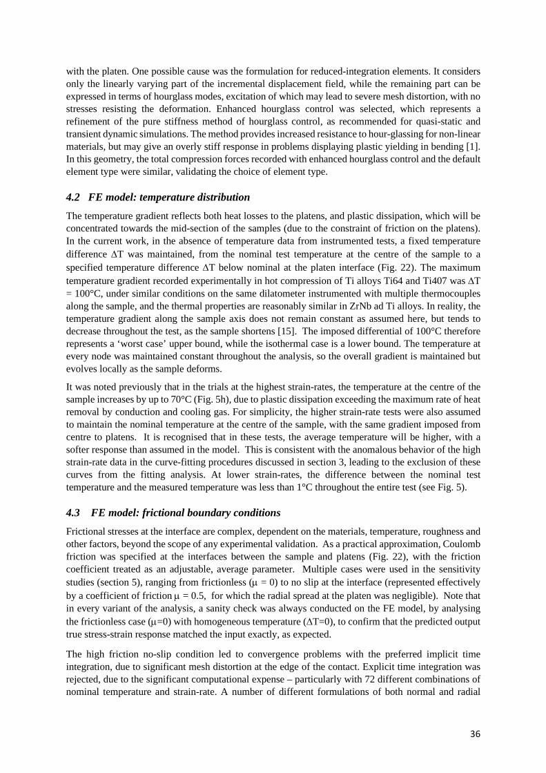
36

with the platen. One possible cause was the formulation for reduced-integration elements. It considers only the linearly varying part of the incremental displacement field, while the remaining part can be expressed in terms of hourglass modes, excitation of which may lead to severe mesh distortion, with no stresses resisting the deformation. Enhanced hourglass control was selected, which represents a refinement of the pure stiffness method of hourglass control, as recommended for quasi-static and transient dynamic simulations. The method provides increased resistance to hour-glassing for non-linear materials, but may give an overly stiff response in problems displaying plastic yielding in bending [1]. In this geometry, the total compression forces recorded with enhanced hourglass control and the default element type were similar, validating the choice of element type. 4.2 FE model: temperature distribution

The temperature gradient reflects both heat losses to the platens, and plastic dissipation, which will be concentrated towards the mid-section of the samples (due to the constraint of friction on the platens). In the current work, in the absence of temperature data from instrumented tests, a fixed temperature difference ∆T was maintained, from the nominal test temperature at the centre of the sample to a specified temperature difference ∆T below nominal at the platen interface (Fig. 22). The maximum temperature gradient recorded experimentally in hot compression of Ti alloys Ti64 and Ti407 was ∆T = 100°C, under similar conditions on the same dilatometer instrumented with multiple thermocouples along the sample, and the thermal properties are reasonably similar in ZrNb ad Ti alloys. In reality, the temperature gradient along the sample axis does not remain constant as assumed here, but tends to decrease throughout the test, as the sample shortens [15]. The imposed differential of 100°C therefore represents a ‘worst case’ upper bound, while the isothermal case is a lower bound. The temperature at every node was maintained constant throughout the analysis, so the overall gradient is maintained but evolves locally as the sample deforms.

It was noted previously that in the trials at the highest strain-rates, the temperature at the centre of the sample increases by up to 70°C (Fig. 5h), due to plastic dissipation exceeding the maximum rate of heat removal by conduction and cooling gas. For simplicity, the higher strain-rate tests were also assumed to maintain the nominal temperature at the centre of the sample, with the same gradient imposed from centre to platens. It is recognised that in these tests, the average temperature will be higher, with a softer response than assumed in the model. This is consistent with the anomalous behavior of the high strain-rate data in the curve-fitting procedures discussed in section 3, leading to the exclusion of these curves from the fitting analysis. At lower strain-rates, the difference between the nominal test temperature and the measured temperature was less than 1°C throughout the entire test (see Fig. 5). 4.3 FE model: frictional boundary conditions

Frictional stresses at the interface are complex, dependent on the materials, temperature, roughness and other factors, beyond the scope of any experimental validation. As a practical approximation, Coulomb friction was specified at the interfaces between the sample and platens (Fig. 22), with the friction coefficient treated as an adjustable, average parameter. Multiple cases were used in the sensitivity studies (section 5), ranging from frictionless (µ = 0) to no slip at the interface (represented effectively by a coefficient of friction µ = 0.5, for which the radial spread at the platen was negligible). Note that in every variant of the analysis, a sanity check was always conducted on the FE model, by analysing the frictionless case (µ=0) with homogeneous temperature (∆T=0), to confirm that the predicted output true stress-strain response matched the input exactly, as expected.

The high friction no-slip condition led to convergence problems with the preferred implicit time integration, due to significant mesh distortion at the edge of the contact. Explicit time integration was rejected, due to the significant computational expense – particularly with 72 different combinations of nominal temperature and strain-rate. A number of different formulations of both normal and radial

37

behavior at the interface were systematically tested. Various frictional implementations were tested, including different frictional constraint enforcement methods (penalty or Lagrange multiplier methods), a range of values of a friction coefficient with allowable elastic slip, and a formulation with friction coefficient decaying exponentially from the static value to the kinetic value. Four types of contact pressure-overclosure relationships were assessed – a “hard” relationship, which minimized the penetration, and three types of “softened” contact relationships: linear, piecewise-linear, and exponential. A no-separation relationship, preventing surface separation once they have come into contact, was also checked. Finally, three contact constraint enforcement methods were tested: direct, penalty, and augmented Lagrange. Contact constraint enforcement methods determine how contact constraints imposed by a physical pressure-overclosure relationship are resolved numerically [27].

All the formulations were assessed in terms of achieving convergence, the computational expense, and a comparison of the total compression force with that obtained using the default contact formulation. Each contact formulation was tested at the maximum and minimum experimental strain-rate, as the strain-rate was found to affect the convergence. The convergence problems were finally solved across all test conditions using a contact relationship in which the contact pressure was a user-defined piecewise linear function of the clearance between the surfaces. In Abaqus, a contact pressure-overclosure relationship can be defined as “hard” or “softened”. The “hard” relationship minimizes the penetration of the surfaces – when the surfaces are in contact, any pressure can be transmitted between them with zero-penetration (although the zero-penetration condition may not be strictly enforced). In a “softened” contact relationship, contact pressure is a function of the clearance between the surfaces. In the current model, a pressure-overclosure relationship was defined as piecewise-linear in tabular form, by specifying data pairs of increasing pressure versus overclosure (where overclosure corresponds to negative clearance). “Softened” contact relationships of this type are sometimes useful to resolve numerical issues with contact conditions [28].

As a result, note that the distribution of stresses at the platen interface may not be very reliable. However, this is not significant in the current problem, because: (a) the friction and temperature gradient mean that the stresses at the platen are mostly below yield, giving a “dead metal zone” with limited radial strain; (b) the mid-section of the sample is fully yielding, and the conditions here determine the net force at a given displacement. The pressure distribution at the platen is therefore constrained to be in equilibrium with the correct load, even if the detail of the radial variation is uncertain. This is explored further in Section 5.

5. FE modelling: sensitivity studies

The finite element model was first applied to conduct a range of sensitivity studies into the effect of the friction coefficient and temperature gradient (separately and together), and the mesh size and imposed strain-rate. The influence of changing parameters was investigated by comparing the predicted force-displacement responses, the deformed (barrelled) shape, and the spatial inhomogeneity of the deformation within the sample. The isothermal, frictionless case provided the benchmark case for the force-displacement response, being the ideal case in which the input true stress-strain response is constant over the whole sample, and the output stress-strain response is identical to the input.

As a proof of concept, the results presented use the standard ‘worst case’ upper bound discussed above, i.e. a friction coefficient µ = 0.5, and temperature difference ∆T = 100°C (unless stated otherwise). Preliminary analyses all started with the case of nominal temperature 𝑇𝑇nominal = 750°C and nominal strain-rate 𝜀𝜀̇nominal = 0.1 s-1. These correspond to mid-range nominal conditions within the experimental dataset and material constitutive model. The Sellars-Tegart constitutive model fitted by multi-variable regression (section 3.4) was used in the first sensitivity studies, for computational efficiency. The use of a perfectly plastic material response visually highlights the effect of barrelling on the “notional” true stress-strain curve.

38

5.1 Coefficient of friction

Figure 23 shows the impact of friction coefficient on the force-displacement response, and the corresponding notional true stress-strain response, for three physically realistic values of µ = 0.1, 0.3 and 0.5. In order to decouple the effects of friction and temperature gradient, the temperature across the sample was first assumed to be uniform and equal to 𝑇𝑇nominal, with ∆T = 0. For the ideal isothermal and frictionless case (µ = 0), a check was conducted that the predicted true stress-strain response matched the input to the model, as seen in Fig. 23(b).

Figure 23 Predictions of the FE model for isothermal Tnominal = 750°C and 𝜀𝜀̇nominal = 0.1 s-1, for different coefficients of friction: (a) force vs displacement; (b) “notional” true stress vs strain.

As the coefficient of friction increases, the axial force necessary to deform the sample also increases, as expected (Fig. 23a). The notional true stress-strain (Fig. 23b) is calculated from equation (1), assuming that the sample remains cylindrical. Note in particular how friction leads to an apparent hardening response, with a 20% rise in flow stress at µ = 0.5, when the material is in fact perfectly plastic.

Figure 24 shows the corresponding predicted distributions of von Mises equivalent plastic strain. Friction constrains the lateral motion of the material in direct proximity to the platens and leads to ‘dead metal zones’ adjacent to the workpiece-platen interfaces. The unconstrained material at the centre of the sample must be pushed outwards in the radial direction, to accommodate most of the axial change in length of the sample, amplifying the plastic strain.

Figure 24 Von Mises equivalent plastic strain at 𝑇𝑇nominal = 750°C, 𝜀𝜀̇nominal = 0.1 s-1, and 𝜀𝜀nominal = 0.69, with uniform temperature equal to 𝑇𝑇nominal, and coefficient of friction of: (a) 0.1; (b) 0.3; (c) 0.5.

Maps of axial and radial strain-rate (Fig. 25) provide further insight, highlighting the dead metal zones and corresponding amplification of the axial strain-rate compared to the nominal value, with the appearance of shear bands, consistent with the formation of the barrelled shape.

0

1

2

3

4

5

6

7

0 2 4 6

Forc

e [k

N]

Displacement [mm]

00.10.30.5

0

50

100

150

0 0.2 0.4 0.6 0.8

Flow

str

ess [

MPa

]

True strain

FE model, mu=0.5FE model, mu=0.3FE model, mu=0.1FE model, mu=0

Coefficient of friction (a) (b)

Equivalent plastic strain

(a) (b) (c)

Coefficient of friction

39

Figure 25 Axial (a-c) and radial (d-f) strain-rates at uniform Tnominal = 750°C, 𝜀𝜀̇nominal = 0.1 s-1, and 𝜀𝜀nominal = 0.69, for three values of coefficient of friction µ.

5.2 Temperature gradient

The effect of temperature gradient is first investigated assuming frictionless interfaces, with the mid-plane temperature equal to 𝑇𝑇nominal, and an initial linear decrease to (𝑇𝑇nominal − ∆𝑇𝑇) at the workpiece-platen interfaces (Fig. 22). The temperature at each node then remains constant throughout the analysis. Three different values of ∆𝑇𝑇 were tested: 25, 50 and 100°C.

Figure 26 shows that a temperature gradient also produces barrelling, even in the absence of friction, and the extent of barrelling increases with ∆𝑇𝑇. The softer central region expands laterally more easily, with the colder regions near the interfaces behaving like an extension of the platens. Note the difference in the barrelled shape compared to that produced by friction alone (Fig. 24) – in Fig. 26 the curvature goes through a point of inflection, and more closely resembles the cross-section observed experimentally (Fig. 3b). This suggests that the temperature gradient is important in determining the deformation of the dilatometer specimens.

Figure 26 Temperature distribution at Tnominal = 750°C, 𝜀𝜀̇nominal = 0.1 s-1, and 𝜀𝜀nominal = 0.69, with ∆T equal to: (a) 25°C; (b) 50°C; (c) 100°C.

Axial strain rate [s-1]

Radial strain rate [s-1]

(a) (b) (c)

(d) (e) (f)

Temperature [°C]

(a) (b) (c)

µ = 0.1 µ = 0.3 µ = 0.5

40

The FE model also shows that the temperature gradient has a different effect compared to friction on the force-displacement and stress-strain curves. The axial force rises with the temperature differential along the sample (Fig. 27a), while the stress-strain curves (Fig. 27b) exhibit a peak stress up to 30% higher than the nominal value, with apparent hardening followed by softening. Note that this resembles the experimental data (Fig. 8), though the input material response was perfectly plastic.

Figure 27 Predictions of the FE model at Tnominal = 750°C and 𝜀𝜀̇nominal = 0.1 s-1, for different

temperature gradients: (a) force vs displacement; (b) “notional” true stress vs strain.

Figure 28 shows the distribution of plastic strain, again revealing the magnification of strain in the centre and dead metal zones at the interfaces. For a temperature gradient of 100°C (Figure 28c), the dead metal zones are more pronounced than in the high friction case, with a greater increase in the central plastic strain.

Figure 28 Von Mises equivalent plastic strain at Tnominal = 750°C, 𝜀𝜀̇nominal = 0.1 s-1, and 𝜀𝜀nominal = 0.69, with no friction, and temperature gradient ∆T equal to: (a) 25°C; (b) 50°C; (c) 100°C.

The distributions of strain-rate (Figure 29) again highlight the dead metal zones and magnified central axial strain-rate, but with more pronounced shear bands and dead metal zones associated with barrelling being concentrated towards the mid-plane.

0

1

2

3

4

5

6

7

0 2 4 6

Forc

e [k

N]

Displacement [mm]

Uniform T25 deg. C50 deg. C100 deg. C

0°C25°C50°C100°C

0

50

100

150

0 0.2 0.4 0.6 0.8Fl

ow s

tres

s [M

Pa]

True strain

Uniform T25°C50°C100°CZ-H model

FE input0°C25°C50°C100°C

Equivalent plastic strain

(a) (b) (c)

(a) (b)

Temperature gradient

Temperature gradient

41

Figure 29 Axial (a-c) and radial (d-f) components of strain-rate at Tnominal = 750°C,

𝜀𝜀̇nominal = 0.1 s-1, and 𝜀𝜀nominal = 0.69, with no friction, for 3 values of temperature gradient ∆T.

5.3 Combined effects of friction and temperature gradient

In practice both friction and temperature gradients act simultaneously, hence the combined effect was investigated. Upper and lower bound combinations were analysed, with coefficients of friction of 0.1 and 0.5, and temperature gradients of 25°C and 100°C. Figure 30 shows the combined effect on force-displacement and stress-strain responses.

Figure 30 suggests that the effect of temperature gradient is apparent immediately at low strain, but the curves then also diverge for different values of friction coefficient. The high friction stress-strain curves show apparent hardening, the lower friction cases show a transition to approximately constant flow stress. For the values chosen, the final influence of friction and temperature gradient on flow stress are of comparable magnitude, with the apparent flow stress being substantially higher (around 60%) than the nominal value, for high friction and the greatest temperature difference.

Figure 30 FE model predictions at Tnominal = 750°C, 𝜀𝜀̇nominal = 0.1 s-1, for 4 combinations of friction coefficient and temperature gradient: (a) force vs displacement; (b) “notional” true stress vs strain.

0

1

2

3

4

5

6

7

0 2 4 6

Forc

e [k

N]

Displacement [mm]

μ=0.1; ΔT=25°Cμ=0.5; ΔT=25°Cμ=0.1; ΔT=100°Cμ=0.5; ΔT=100°C

µ=0.1; ∆T=25°Cµ=0.5; ∆T=25°Cµ=0.1; ∆T=100°Cµ=0.5; ∆T=100°C

0

50

100

150

200

0 0.2 0.4 0.6 0.8

Flow

str

ess [

MPa

]

True strain

Z-H modelμ=0.1; ΔT=25°Cμ=0.5; ΔT=25°Cμ=0.1; ΔT=100°Cμ=0.5; ΔT=100°C

FE inputµ=0.1; ∆T=25°Cµ=0.5; ∆T=25°Cµ=0.1; ∆T=100°Cµ=0.5; ∆T=100°C

Axial strain rate [s-1]

Radial strain rate [s-1]

(a) (b) (c)

(d) (e) (f)

(a) (b)

∆T = 25oC ∆T = 50oC ∆T = 100oC

42

Figure 31 shows the final shapes and temperature distribution for the four combinations shown in Fig, 30. The undeformed and ‘ideal’ (average) deformed radii are super-imposed. These reference shapes help to visualize the separate influences of friction and temperature gradient on the behaviour. The final contact radius is dominated by friction, with a secondary influence of the temperature gradient; the maximum radius of the barrelled region is affected equally by both.

0

Figure 31 Temperature distributions at Tnominal = 750°C, 𝜀𝜀̇nominal = 0.1 s-1, and 𝜀𝜀nominal = 0.69, for different combinations of friction coefficient and temperature gradient: (a) µ=0.1, ∆T=25°C;

(b) µ=0.5, ∆T=25°C; (c) µ=0.1, ∆T=100°C; (d) µ=0.5, ∆T=100°C.

The distributions of von Mises equivalent plastic strain (Fig. 32) and strain-rate (Fig. 33) are similar to those shown in the previous sections, with dead metal zones, centrally amplified axial strain and strain-rate, and shear bands. The maximum values of both plastic strain and axial strain-rate at the centre are approximately twice the nominal values.

Figure 32 Von Mises equivalent plastic strain at Tnominal = 750°C, 𝜀𝜀̇nominal = 0.1 s-1, and 𝜀𝜀nominal = 0.69, for different combinations of friction coefficient and temperature gradient: (a) µ=0.1, ∆T=25°C;

(b) µ=0.5, ∆T=25°C; (c) µ=0.1, ∆T=100°C; (d) µ=0.5, ∆T=100°C.

(a) (b) (c) (d)

(a) (b) (c) (d)

Temp. [°C]

Eq. plastic strain

R0

RAVG RAVG

R0

RAVG

R0

RAVG

R0

43

Figure 33 Axial (a-d) and radial (e-h) components of strain-rate at Tnominal = 750°C, 𝜀𝜀̇nominal = 0.1 s-1, and 𝜀𝜀nominal = 0.69, for different combinations of friction coefficient and temperature gradient.

5.4 Mesh size

The sensitivity studies above, assessing the influence of friction and temperature gradient, used a relatively large mesh size, for faster computation, and to give clearer visualisation of the temperature and deformation with the mesh superimposed. But mesh sensitivity and accuracy become more critical when the FE model is applied to predict the experimental data, and to correct the stress-strain response. The model also has to be computationally efficient, due to the large number of test conditions, and the requirement to run the model more than once per test. Hence the mesh sensitivity was first tested using the case with the most severe friction coefficient and temperature gradient (µ=0.5, ∆T=100°C). The study was also extended to the limiting strain-rates, to be sure that the analysis was robust over the full experimental domain.

Figure 34 shows force-displacement and stress-strain curves for different numbers of elements, ranging from 100 to 25600. It indicates that the minimum number of elements is roughly 1600, at which the results start to converge. As shown in Fig. 35, this number of elements is also reasonable in terms of computational speed (of the order of one minute).

Figure 34 FE results at Tnominal = 750°C and 𝜀𝜀̇nominal = 0.1 s-1, with µ=0.5 and ∆T=100°C, for different

number of elements: (a) force vs displacement; (b) notional true stress vs strain.

0

1

2

3

4

5

6

7

0 0.002 0.004 0.006

Forc

e [k

N]

Displacement [mm]

1004001600320064001280025600

Number ofelements

0

50

100

150

200

0 0.2 0.4 0.6 0.8

Flow

str

ess [

MPa

]

True strain

Input1004001600320064001280025600

Number ofelements

(a) (b) (c) (d)

(e) (f) (g) (h)

Axial strain rate [s-1]

Radial strain rate [s-1]

(a) (b)

µ=0.1, ∆T = 25oC µ=0.5, ∆T = 25oC µ=0.1, ∆T = 100oC µ=0.5, ∆T = 100oC

0 2 4 6

44

Figure 35 Simulation time vs number of elements, for the analyses of Fig. 34.

Figure 36 and 37 shows the distribution of equivalent plastic strain and stress, respectively, for different values of mesh size, which has a clear influence on both the overall shape of deformed sample, and the maximum value of plastic strain. Again, the results appear to be unchanged above about 1600 elements, confirming the conclusion drawn from the force-displacement curves.

Figure 36 Von Mises equivalent plastic strain at Tnominal = 750°C, 𝜀𝜀̇nominal = 0.1 s-1, and 𝜀𝜀nominal = 0.69, with µ=0.5 and ∆T=100°C, for different numbers of elements:

(a) 100; (b) 400; (c) 1600; (d) 3200; (e) 6400; (f) 25600.

1

10

100

1000

10000

1 10 100 1000 10000 100000

Sim

ulat

ion

time

[s]

Number of elements

(c)

Eq. plastic strain

(a) (b) (c)

(d) (e) (f)

45

Figure 37 Von Mises equivalent stress at Tnominal = 750°C, 𝜀𝜀̇nominal = 0.1 s-1, and 𝜀𝜀nominal = 0.69, with µ=0.5 and ∆T=100°C, for different numbers of elements:

(a) 100; (b) 400; (c) 1600; (d) 3200; (e) 6400; (f) 25600.

Figure 34 showed a large difference between force-displacement and stress-strain curves obtained with small (100-400) and large (>1600) number of elements. Figures 36 and 37 reveal why – beyond a certain mesh size, the stress-strain conditions stabilise across the mid-section, and across the platen interface, corresponding to the convergence of the force-displacement curves with increasing mesh size. Since increasing the mesh size reduces the magnitude of the force-displacement curve, the influence of combinations of friction coefficient and temperature gradient were re-evaluated with the fine mesh (1600 elements). Comparing with Fig. 30 (using a coarse mesh), Fig. 38 shows that using 1600 elements gives predicted responses that show little dependence of friction coefficient, and only a dependence on temperature gradient.

Figure 38 Predictions of the FE model at Tnominal = 750°C, 𝜀𝜀̇nominal = 0.1 s-1, with 1600 elements, for different combinations of temperature gradient and friction coefficient: (a) force vs displacement;

(b) “notional” true stress vs strain.

0

1

2

3

4

5

6

7

0 0.002 0.004 0.006

Forc

e [k

N]

Displacement [mm]

μ=0.5; ΔT=100°Cμ=0.5; ΔT=25°Cμ=0.1; ΔT=100°Cμ=0.1; ΔT=25°C

(a)

0

50

100

150

200

0 0.2 0.4 0.6 0.8

Flow

str

ess [

MPa

]

True strain

Inputμ=0.5; ΔT=100°Cμ=0.5; ΔT=25°Cμ=0.1; ΔT=100°Cμ=0.1; ΔT=25°C

(b)

Von Mises Stress [Pa]

(a) (b) (c)

(d) (e) (f)

0 2 4 6

46

Closer examination of Fig. 36 shows that the coarsest mesh (Fig. 36a) shows a uniform equivalent stress distribution under the platen, while the fine mesh cases show high peak stresses at the edge of the contact (a numerical artefact due to mesh distortion, and the high friction coefficient). Figure 34 showed that the overall force-displacement curves are smooth, and converge at a mesh with around 1600 elements. An important part of the analysis is the prediction of the total load (to correct the constitutive response). So given the variable pattern of equivalent stress near the platen, and the peak at the edge, a further check was conducted, investigating the normal pressure distribution.

Figure 39 shows the pressure as a function of radius, for the same conditions as in Figs. 34-37, but now including a lower level of strain (0.29) as well as the same final strain (0.69). For the lower strain, Fig. 39(a) shows a small degree of mesh dependence below 1600 elements, and then convergence (consistent with the force or stress at that strain. At the final strain however (Fig. 39b), a pressure spike develops at the edge over the last element or so. This is clearly a numerical artefact associated with mesh distortion, and is consistent with the elevated equivalent stress. The peak stress remains finite however, and the load-displacement curve does not deviate towards high strains (Fig. 38a). So the pressure distribution remains in equilibrium with the total load, when integrated over the platen surface, but is unreliable in its profile with radius. The load remains stable with strain however, since it must also be in equilibrium with the vertical stress on the horizontal mid-section of the sample, where there are no issues with mesh distortion or contact. The inaccuracy in the pressure distribution will not influence the stress state in the plastic region in the middle part of the sample, so the total load and the deformation history at an close to the mid-section are reliable – particularly as both are found to be independent of mesh size above around 1600 elements.

Note in passing that the pressure distribution at low strain (Fig. 39a) is predicted to be an inverse friction hill. This is in contrast to the classical analytical solution, in which pressure rises to a peak at the centre of a circular billet subject to radial friction. However, this solution neglects barrelling, and imposes yield everywhere, when in reality the stress state near the platens is below yield, producing the dead metal zones. Inverse friction hill pressure distributions have been observed previously in FE analyses of simple upsetting, with pressures rising towards the edge – an early example is [29].

Figure 39 Pressure distribution across the platen-workpiece interface for different numbers

of elements, for Tnominal = 750°C, 𝜀𝜀̇nominal = 0.1 s-1, with µ=0.5 and ∆T=100°C, at overall true strains of: (a) 0.29; (b) 0.69.

5.5 Mesh size and strain-rate

The mesh sensitivity study was extended to the upper and lower strain-rates in the current work: 0.0032s-1 and 10s-1. To confirm the choice of 1600 elements, the results were compared for numbers of elements a factor of two either side of this value, 800 and 3200 elements, for which the differences should be modest. Figure 40 shows stress-strain curves for these four cases, calculated in the usual way. The difference between 800 and 3200 elements is small, and significantly smaller than the difference

(b)

0

100

200

300

400

500

600

700

800

900

1000

0 0.5 1 1.5 2 2.5 3

Pres

sure

[MPa

]

Distance from axis [mm]

1004001600320064001280025600

(a)

0

100

200

300

400

500

600

700

800

900

1000

0 0.5 1 1.5 2 2.5 3

Pres

sure

[MPa

]

Distance from axis [mm]

1004001600320064001280025600

47

between input and output. Figures 41-43 also confirm that, at both upper and lower limiting strain-rates, the differences are small between 800 and 3200 elements, in terms of overall shape, and in the final distributions of temperature, von Mises equivalent strain, and axial strain-rate components, are minor. Furthermore, these figures show a high degree of kinematic self-similarity in the deformation field, which is almost independent of the imposed strain-rate (largely a reflection of the identical friction and temperature profile in all cases).

Figure 40 “Notional” true stress-strain curves predicted by the FE model for Tnominal = 750°C, temperature gradient ∆T=100°C, friction coefficient µ=0.5, using 800 and 3200 elements, for nominal

strain-rates of: (a) 𝜀𝜀̇nominal = 0.0032s-1; (b) 𝜀𝜀̇nominal = 10s-1.

Figure 41 Temperature distribution at Tnominal = 750°C and 𝜀𝜀nominal = 0.69, for temperature gradient ∆T=100°C and µ=0.5, with different nominal strain-rates and numbers of elements.

0

50

100

150

200

250

0 0.2 0.4 0.6 0.8

Flow

str

ess [

MPa

]

True strain

FE model (3200 elements)FE model (800 elements)Z-H model

3200800FE Input

Number of elementsFE Input8003200

0

50

100

150

200

250

0 0.2 0.4 0.6 0.8

Flow

str

ess [

MPa

]True strain

FE model (3200 elements)Fe model (800 elements)Z-H model

3200800FE Input

Number of elementsFE Input8003200

(a) (b)

(a) (b)

(c) (d)

�̇�𝜺𝒏𝒏𝒏𝒏𝒏𝒏𝒏𝒏𝒏𝒏𝒏𝒏𝒏𝒏=0.0032 s-1 �̇�𝜺𝒏𝒏𝒏𝒏𝒏𝒏𝒏𝒏𝒏𝒏𝒏𝒏𝒏𝒏=10 s-1

800 elements

3200 elements

48

Figure 42 Von Mises equivalent plastic strain at Tnominal = 750°C and 𝜀𝜀nominal = 0.69, for temperature gradient ∆T=100°C and µ=0.5, for different nominal strain-rates and numbers of elements.

Figure 43 Axial component of strain rate at Tnominal = 750°C and 𝜀𝜀nominal = 0.69, for ∆T=100°C and µ=0.5, with different nominal strain-rates and numbers of elements.

Equivalent plastic strain

(a) (b)

(a) (b)

(c) (d)

(c) (d)

800 elements

3200 elements

�̇�𝜺𝒏𝒏𝒏𝒏𝒏𝒏𝒏𝒏𝒏𝒏𝒏𝒏𝒏𝒏=0.0032 s-1 �̇�𝜺𝒏𝒏𝒏𝒏𝒏𝒏𝒏𝒏𝒏𝒏𝒏𝒏𝒏𝒏=10 s-1

3200 elements

800 elements

�̇�𝜺𝒏𝒏𝒏𝒏𝒏𝒏𝒏𝒏𝒏𝒏𝒏𝒏𝒏𝒏=0.0032 s-1 �̇�𝜺𝒏𝒏𝒏𝒏𝒏𝒏𝒏𝒏𝒏𝒏𝒏𝒏𝒏𝒏=10 s-1

Axial strain rate [s-1]

Axial strain rate [s-1]

49

5.6 Repeat analysis using smoothed experimental stress-strain data

So far, all initial studies used a perfectly plastic Arrhenius-type material model, which provided computational efficiency in testing the sensitivity of the model and visualising changes in the resulting notional true stress-strain curves and the distribution of deformation. However, as discussed earlier in section 3, for accuracy and stability the final FE model uses smoothed raw experimental stress-strain data. This new material model was tested with a number of repeat analyses, covering the same combinations of friction coefficient and temperature gradient as before.

First, a check was performed on the choice of the number of elements. Figure 44 shows that the force vs displacement curves converged again around 1600 elements. A standard mesh size of 1600 elements was again adopted, being the optimal value from the previous study.

Figure 44 Force vs displacement curves predicted by the FE model for different numbers of

elements, with smoothed experimental stress-strain data, for Tnominal = 750°C and 𝜀𝜀̇nominal = 0.1 s-1, with µ=0.5 and ∆T=100°C: (a) force vs displacement; (b) stress vs strain.

The second check was to see if the radial distribution of pressure showed the same numerical artefact at large strains as observed in the previous analysis – see Fig. 45. As before, the pressure spike at large strain (Fig. 45b) is a consequence of the mesh distortion, and also the method adopted for handling friction at the interface to avoid convergence problems. The anomaly in pressure decreases with friction coefficient (disappearing completely with a frictionless interface). The temperature gradient again has a minor impact on this artificial pressure spike. It was also found that the pressure spike only appeared for a mesh size of 400 elements or more, and became narrower and higher as the element size reduced. However, the pressure spike had no impact on the predicted force and stress curves (Fig. 46). This is because the net force must be in equilibrium with the yielding conditions across the mid-section, so the pressure distribution is constrained to deliver the same net force – it does not determine the net force. So while the p(r) variation is physically inaccurate, it does not influence the accuracy of the correction of the constitutive response, nor does it influence the prediction of deformation conditions in the plastic zone around the mid-section, which is the region of interest for microstructural studies.

0

1

2

3

4

5

6

7

0 2 4 6

Forc

e [k

N]

Displacement [mm]

1004001600320064001280025600

0

50

100

150

200

0 0.2 0.4 0.6 0.8

Stre

ss [M

Pa]

Strain

1004001600320064001280025600

(b) (a)

50

Figure 45 Pressure distributions obtained with smoothed experimental stress-strain data across the

platen-workpiece interface at Tnominal = 750°C, 𝜀𝜀̇nominal = 0.1 s-1, with 1600 elements, for different µ and ∆T, and (a) 𝜀𝜀nominal = 0.29; (b) 𝜀𝜀nominal = 0.69.

Figure 46 shows the force-displacement curves obtained with the model, for the 4 combinations of friction coefficient and temperature gradient tested previously. While temperature gradient, as expected, substantially increased the axial force from the onset of deformation, friction was found to have less influence on the axial force, consistent with the results obtain with an Arrhenius type model (compare with Fig. 38). And again a sanity check of the FE model, with the smoothed experimental stress-strain data used as the input, showed that the input response was reproduced exactly for the case of homogeneous temperature and no friction.

Figure 46 Predictions of the FE model with smoothed experimental stress-strain data, at Tnominal = 750°C, 𝜀𝜀̇nominal = 0.1 s-1 and with 1600 elements, for different combinations of temperature gradient

and friction coefficient: (a) force vs displacement; (b) “notional” true stress vs strain

Figures 47-49 show the expected deformation behaviour: dead metal zones close to the sample-platen interfaces, and a region of intense plastic deformation in the centre. With smoothed experimental 𝜎𝜎(𝑇𝑇, 𝜀𝜀, 𝜀𝜀̇), the problems with convergence described in sections 3 were avoided. The deformation patterns evolve with friction and temperature gradient in much the same way as observed at lower mesh resolution using the perfectly plastic. Figure 49 shows that the maximum plastic strain and strain-rate are of the order of 0.3–0.4 times the nominal test value.

0

100

200

300

400

500

600

700

0 1 2 3

Pres

sure

[MPa

]

Distance from axis [mm]

µ=0.5, ΔT=100°Cµ=0.1, ΔT=100°Cµ=0.5, ΔT=25°Cµ=0.1, ΔT=25°C

0

100

200

300

400

500

600

700

0 1 2 3 4

Pres

sure

[MPa

]

Distance from axis [mm]

µ=0.5, ΔT=100°Cµ=0.1, ΔT=100°Cµ=0.5, ΔT=25°Cµ=0.1, ΔT=25°C

0

1

2

3

4

5

6

7

0 2 4 6

Forc

e [k

N]

Displacement [mm]

µ=0.5, ΔT=100°Cµ=0.1, ΔT=100°Cµ=0.5, ΔT=25°Cµ=0.1, ΔT=25°C 0

50

100

150

200

0 0.2 0.4 0.6 0.8

Stre

ss [M

Pa]

Strain

µ=0.5, ΔT=100°Cµ=0.1, ΔT=100°Cµ=0.5, ΔT=25°Cµ=0.1, ΔT=25°C

51

Figure 47 von Mises equivalent plastic strain obtained with smoothed experimental stress-strain data at Tnominal = 750°C, 𝜀𝜀̇nominal = 0.1 s-1, and 𝜀𝜀nominal = 0.69, with 1600 elements, for different combinations

of friction coefficient and temperature gradient.

Figure 48 von Mises equivalent stress obtained with smoothed experimental stress-strain data

at Tnominal = 750°C, 𝜀𝜀̇nominal = 0.1 s-1, and 𝜀𝜀nominal = 0.69, with 1600 elements, for different combinations of friction coefficient and temperature gradient.

Equivalent plastic strain

(b)

von Mises Stress [Pa]

(a)

(d) (c)

∆Τ = 100°C

∆Τ = 25°C

µ=0.1 µ=0.5

µ=0.1 µ=0.5

∆Τ = 100°C

∆Τ = 25°C

(a) (b)

(c) (d)

52

Figure 49 FE results obtained with smoothed experimental stress-strain data at Tnominal = 750°C,

𝜀𝜀̇nominal = 0.1 s-1, and 𝜀𝜀nominal = 0.69, with µ=0.5 and ∆T=100°C, with 1600 elements: (a) temperature; (b) equivalent plastic strain; (c) von Mises stress; (d) axial strain-rate; (e) radial strain-rate.

5.7 Summary of finite element sensitivity analysis

To conclude the sensitivity analyses of deformation conditions in the dilatometer, the following observations have been made:

• barrelling results from both friction and a temperature gradient, with a gradient ∆T=100oC having a more prominent role than a high friction coefficient µ=0.5;

• the strain and strain-rate distribution around the mid-section of the sample is inhomogeneous, with peak values around 0.3–0.4 times the nominal test values, and significant dead metal zones at either end;

• microstructural interpretation of dilatometer samples (or crystal plasticity analyses of the central region) must take due account of the inhomogeneity in the deformation conditions;

• the notional true stress-strain response inferred directly from the load-displacement curves is substantially different from the true material response, and needs to be corrected (see section 6);

• broadly similar conclusions could be reached using both a perfectly plastic constitutive response, and using the notional true stress-strain response from the experiments, suitably smoothed;

• there were some computational issues associated with mesh distortion at large strains, and with the implementation of friction, leading to non-physical spikes in pressure at the outer edge of the contact area with the platen, at large strains; however, the total load and the deformation distribution around the mid-section were considered to be reliable (as both are governed by the plastic deformation behaviour in the mid-section).

Equiv. plastic strain

von Mises Stress [Pa]

Temp. [°C]

Axial strain rate [s-1]

Radial strain rate [s-1]

(a) (b) (c)

(d) (e)

53

6. Constitutive data correction method

As summarised in section 1.4, the objective of the analysis presented in this report is to develop a numerical scheme for inferring the uniaxial true stress-strain response, by applying a systematic correction to the ‘notional’ true stress-strain response taken directly from the test data, to account for the influence of friction and inhomogeneous temperature. This then enables the deformation history to be predicted at every point in the sample, for interpretation and modelling of the microstructural evolution. In the first instance, the analysis uses the perfectly plastic Sellars-Tegart model, as the simplest dataset capturing the temperature and strain-rate dependence of flow tress for this alloy (Fig. 17). Subsequently, the analysis used the smoothed experimental stress-strain data (Fig. 20), and tested the precision with which it was necessary to capture the stress correction ∆𝜎𝜎 = 𝑓𝑓(𝑇𝑇, 𝜀𝜀̇, 𝜀𝜀). All analyses were initially conducted using the nominal boundary conditions of a friction coefficient µ = 0.5 and fixed temperature gradient ∆T = 100oC. In the final analysis, this was adjusted to ∆T = 50oC, reflecting recent experimental results on Ti alloys that indicate a lower temperature gradient. As the actual temperature gradient is unknown in the ZrNb experiments, and evolves during the test, the “corrected” stress-strain data and predictions of deformation histories are not accurate, and should only be regarded as a proof of concept.

6.1 Correction method applied using Arrhenius-type material model

The correction procedure, presented in Figure 2, was first applied to a 2×2 matrix of tests, chosen with conditions that fell inside the upper and lower limits of both temperature and strain-rate: 700 and 800oC, 0.01 and 3.2s-1. The correction required at each strain was fitted to a best fit surface ∆𝜎𝜎 = 𝑓𝑓(𝑇𝑇, 𝜀𝜀̇), and the corrected stress-strain response interpolated at an intermediate 𝑇𝑇 and 𝜀𝜀̇, giving a 3×3 matrix of conditions. The avoidance of limiting values of 𝑇𝑇 and 𝜀𝜀̇, is because the real tests experience 𝑇𝑇 and 𝜀𝜀̇ distributions above and below the nominal values, so the 3×3 test matrix minimised the extrapolation of the input response beyond the range of the data to which it was fitted, when modelling the non-uniform conditions in the tests. Note however that in all cases, extrapolation to zero strain-rate is an inevitable consequence of the formation of a dead metal zone (as discussed in section 3.6).

Here we use the perfectly plastic model Arrhenius-type (Sellars-Tegart) model from section 3.4. This was fitted to the experimental data at low strain, and is readily extrapolated to cover the necessary ranges of temperatures and strain-rates (Fig. 21a). The model was used as input to the FE analysis to generate the stress correction surfaces, to see if the offset due to inhomogeneous deformation in the sample can be evaluated without taking account of material hardening or softening.

Figure 47 shows the FE predicted input and output responses, for the 2×2 matrix of conditions, presented as “notional” true stress-strain curves. The offset in stress, ∆𝜎𝜎, is the difference between the curves, and varies with test conditions and with strain.

The correction stress was evaluated at strain intervals of 0.05, and planar surface fits for ∆𝜎𝜎(𝑇𝑇, 𝜀𝜀̇) were made by regression analysis using the 4 values obtained at each strain. Figure 48 shows the resulting surfaces at a low and a high strain, with the original data highlighted. A planar fit is as high order as can be justified with only 4 points, and the agreement with the data is good, particularly at low strain. The correction increases with decreasing temperature and with increasing strain-rate, and varies with strain. It is difficult to draw any physical conclusions about these dependencies, since the stress correction depends on the complete distribution of deformation in the sample, and will indeed also depend on the assumed input constitutive response. The magnitude of the correction is significant – up to 70MPa at the high strain-rate end – but the significance of the correction must be considered relative to the magnitude of the absolute stress that is being corrected (see below).

54

Figure 47 Stress-strain curves used as input to the FE analysis (red curve, from perfectly plastic Sellars-Tegart model) vs. FE predicted output (dashed blue curve) for the dilatometer tests with

inhomogeneous deformation, for selected nominal temperatures and strain-rates.

Figure 48 Stress correction ∆𝜎𝜎 as a function of temperature T and log(strain-rate, 𝜀𝜀̇), using the perfectly plastic Sellars-Tegart model as input to the FE analysis, for strains of:

(a) 𝜀𝜀=0.05; (b) 𝜀𝜀=0.5. FE predicted values (red circles), and best-fit planes (blue circles).

0

50

100

150

200

250

300

350

Stre

ss [M

Pa]

0

50

100

150

200

250

300

350

0 0.2 0.4 0.6 0.8

Stre

ss [M

Pa]

Strain0 0.2 0.4 0.6 0.8

Strain

0.01s-1 3.2s-1

700°C

800°C

(b) (a)

log(strain rate) log(strain rate)

55

Using the surfaces for ∆𝜎𝜎(𝑇𝑇, 𝜀𝜀̇) at each strain, the constitutive response from the smoothed experimental data was then corrected to give a new look-up table of stress-strain data 𝜎𝜎 = 𝑓𝑓(𝑇𝑇, 𝜀𝜀̇, 𝜀𝜀), for test temperatures and strain-rates within the ranges used to fit the correction (as in Fig. 47). The value of ∆𝜎𝜎 is subtracted from the original value at each point, to compensate for the over-estimate of stress predicted by the FE analysis.

The test of the corrected data is then to use this as input to the FE model, to see if it can re-predict the experiments, but now capturing the inhomogeneity in deformation. To do this however, the constitutive response must cover extrapolations in temperature and strain-rate – in particular down to zero strain-rate. There is no guarantee that the surface fits to ∆𝜎𝜎(𝑇𝑇, 𝜀𝜀̇) may be extrapolated reliably, but in the first instance the correction surface for each strain (as in Fig. 48) was applied to the smoothed experimental data over the entire domain of temperature and strain-rate of Fig. 21b.

Figure 49 shows the uncorrected and corrected data, at the same strain values as in Fig. 48. The offset downwards is apparent in all cases, with the ratio of corrected to uncorrected for low test temperatures being typically around 80% for all strain-rates. However, at high strain the curve for the lowest strain-rate approaches zero flow stress at the top temperature – further extrapolation to lower strain-rates (or higher temperatures) would lead to non-physical negative values of stress, as a result of the extrapolated correction ∆𝜎𝜎(𝑇𝑇, 𝜀𝜀̇) becoming greater than the extrapolated experimental stress. Extrapolation to a strain-rate of 10-4 s-1 is needed to complete the validation of the method at all nominal test conditions, but led to a number of flow stress values dropping below zero at high temperatures and strains. This reveals a limitation of extrapolating a planar surface fit to the stress-correction. To enable predictions to be completed across the whole experimental domain, the flow stress was assumed to be quasi-static and independent of strain-rate, using the value at the lowest strain-rate that had a positive flow stress.

Figure 49 Uncorrected (left) and corrected (right) flow stress as a function of temperature and strain-rate, for strains of 0.05 (top) and 0.5 (bottom). [Correction computed using the

perfectly plastic Sellars-Tegart model as input to the FE analysis.]

56

The corrected constitutive response was used to predict the notional true stress-strain responses in all 9 combinations of test conditions in the 3×3 matrix of tests (i.e. within the ranges of the original correction cases: 700–800°C, �̇�𝜀=0.01–3.2s-1), with the results shown in Fig. 50. The correction methodology works well at the highest temperature but less so at 700 and 750°C – in all cases a single iteration enables the experimental data to be predicted closely, from a corrected look-up table for uniaxial 𝜎𝜎 = 𝑓𝑓(𝑇𝑇, 𝜀𝜀̇, 𝜀𝜀). Note that not just the magnitude but also the shapes of the initial and corrected curves can differ, so that the interpretation of apparent work hardening or work softening may be significantly modified.

Figure 50 FE predicted stress-strain curves for a 3×3 matrix of temperatures and strain-rates. Solid red: smoothed experimental data; dashed red: corrected input to FE validation; dashed blue: resulting predicted output. [Correction computed using the perfectly plastic Sellars-Tegart model

as input to the FE analysis.]

6.2 Correction method applied using smoothed experimental stress-strain data

Correction using a subset of nominal test conditions

The correction methodology presented so far used the Sellars-Tegart fit to the low strain flow stress data as the starting material model, neglecting the strain-dependence of the flow stress. This was not sufficiently accurate to enable the original experiments to be predicted using a corrected constitutive response; and this response could not be extrapolated to high temperatures and low strain-rates. Here, the analysis is repeated using as input the smoothed experimental data – the data that are to be corrected – but now including strain-dependence.

0

50

100

150

200

250

300

Stre

ss [M

Pa]

0

50

100

150

200

250

300

Stre

ss [M

Pa]

0

50

100

150

200

250

300

0 0.2 0.4 0.6 0.8

Stre

ss [M

Pa]

Strain

0 0.2 0.4 0.6 0.8

Strain

0 0.2 0.4 0.6 0.8

Strain

0.01s-1 0.1s-1 1s-1

700°C

750°C

800°C

57

Figure 51 shows the predicted notional true stress-strain responses for the same 2×2 matrix of tests conditions used earlier (700 and 800oC, 0.01 and 3.2s-1). The correction stress ∆𝜎𝜎(𝑇𝑇, 𝜀𝜀̇) was again fitted to a planar surface by regression analysis using the 4 values obtained at each strain, at strain intervals of 0.05. Compared with Fig. 47, the trends in the stress offsets appear to follow similar trends, but this is not the case, as seen when the stress correction ∆𝜎𝜎 = 𝑓𝑓(𝑇𝑇, 𝜀𝜀̇) is plotted – see Fig. 52. At higher strain, the stress correction now increases with both increasing temperature and strain-rate – the opposite trend with temperature compared to that found using the perfectly plastic model (Fig. 48b).

Figure 51 Stress-strain curves used as input to the FE analysis (red curve, from smoothed fit to experimental data) vs. FE predicted output (dashed blue curve) for the dilatometer tests with

inhomogeneous deformation, for selected nominal temperatures and strain-rates.

Figure 52 Stress correction ∆𝜎𝜎 as a function of temperature 𝑇𝑇 and log(strain rate, 𝜀𝜀̇), using the smoothed experimental data as input to the FE analysis, for strains of:

(a) 𝜀𝜀=0.05; (b) 𝜀𝜀=0.5. FE predicted values (red circles), and best-fit plane (blue circles).

0

50

100

150

200

250

300

Stre

ss [M

Pa]

0

50

100

150

200

250

300

0 0.2 0.4 0.6 0.8

Stre

ss [M

Pa]

Strain0 0.2 0.4 0.6 0.8

Strain

0.01s-1 3.2s-1

700°C

800°C

(b) (a)

log(strain rate) log(strain rate)

58

The extrapolated correction was again applied to the full domain of the experiments, and extended to lower temperatures and strain-rates. Figure 53 shows the uncorrected and corrected flow stress, at the same strain values as Fig. 49. The offset downwards is of a similar order as previously, with the corrected data showing lower sensitivity to strain-rate at low strain. At high temperatures and low strain-rates, the same problem as before is encountered, with the extrapolated correction ∆𝜎𝜎(𝑇𝑇, 𝜀𝜀̇) exceeding the extrapolated experimental stress, leading to non-physical negative values of stress. This now occurs at the lowest experimental strain-rates, not only on extrapolation to 10-4 s-1. The same numerical fix was applied as before, assuming a quasi-static flow stress below the lowest strain-rate for which the flow stress was positive.

Figure 53 Uncorrected (left) and corrected (right) flow stress as a function of temperature and strain-rate, for strains of 0.05 (top) and 0.5 (bottom). [Correction computed using the

smoothed and extrapolated experimental data as input to the FE analysis.]

The corrected constitutive response was again used to predict the notional true stress-strain responses in all 9 combinations of test conditions in the 3×3 matrix of tests (i.e. within the ranges of the original correction cases: 700–800°C, 𝜀𝜀̇=0.01–3.2s-1), with the results shown in Fig. 54. Now the correction methodology works well in all cases – a single iteration enables the experimental data to be predicted closely, validating the corrected look-up table for uniaxial 𝜎𝜎 = 𝑓𝑓(𝑇𝑇, 𝜀𝜀̇, 𝜀𝜀). Note that the magnitude of the correction varies with strain, so that the interpretation of the extent of work hardening or work softening may be significantly modified, as well as the magnitude of the flow stress.

59

Figure 54 FE predicted stress-strain curves for a 3×3 matrix of temperatures and strain-rates: Solid red: smoothed experimental data (also used as initial input to FE to find the correction); dashed

red: corrected input to FE validation; dashed blue: resulting predicted output.

The methodology now appears to be reliable within the range of conditions used to evaluate the stress correction, but has already been seen to break down at high temperatures, due to the simplicity of the planar surface fit used for ∆𝜎𝜎(𝑇𝑇, 𝜀𝜀̇). Nonetheless, the method may be tested at the low temperature end of the experiments. Figure 55 shows the FE predicted notional true stress-strain curves for three strain-rates at 650oC, compared with the smoothed experimental data. The predictions are equally good for the lower two strain-rates, but not for the highest strain-rate – but it should be noted that the experimental data at this strain-rate was in any case previously excluded from the analysis, due to the limitations of the dilatometer. In conclusion therefore, the corrected constitutive response may be inferred beyond the ranges of the experimental data used to fit the correction.

0

50

100

150

200

250

300St

ress

[MPa

]

0

50

100

150

200

250

300

Stre

ss [M

Pa]

0

50

100

150

200

250

300

0 0.2 0.4 0.6 0.8

Stre

ss [M

Pa]

Strain0 0.2 0.4 0.6 0.8

Strain

0 0.2 0.4 0.6 0.8

Strain

0.01s-1 0.1s-1 1s-1

700°C

750°C

800°C

60

Figure 55 FE predicted stress-strain curves for a low temperature of 650°C at selected strain-rates. Solid red: smoothed experimental data (also used as initial input to FE to find the correction);

dashed red: corrected input to FE validation; dashed blue: resulting predicted output.

Even though the correction method works well with the smoothed data as input, there remains the breakdown of the method at high strains and temperatures, at low strain-rates. This is a consequence of using a planar fit to a 2×2 matrix of conditions, and extrapolating in temperature and strain-rate. An alternative procedure would be: (a) to evaluate the correction at all nominal test conditions; (b) to apply these corrections point-by-point to the smoothed experimental data; (c) to repeat the fitting procedure used on the raw experimental data (section 3.5). This would yield a function for log𝜎𝜎 = 𝑓𝑓(𝑇𝑇, log 𝜀𝜀̇) at each strain, rather than a look-up table, and by fitting to log(σ), the possibility of extrapolation to negative stress values is avoided. This approach is tested below. Correction using complete set of nominal test conditions

The analysis of the previous section was repeated, using the smoothed and extrapolated experimental data as input to the FE analysis, with two substantive modifications:

(a) the correction was evaluated for all 72 combinations of temperature and strain-rate in the experimental programme, and no fit was made to this data – the correction was applied cirectly to the initial smoothed experimental data, and then the same smoothing and fitting method re-applied;

(b) the temperature difference from the centre of the sample to the platens was reduced to 50oC.

The second change was a reflection of recent experimental and modelling work on Ti alloys [14]. Even though the gradient was not measured in the ZrNb experiments, the Ti data give a guide, as the thermal properties of ZrNb and Ti alloys are reasonably similar. For the final analysis, a fixed value of 50oC was considered to be more representative of the gradient over the whole matrix of test conditions, including the reduction in the temperature difference observed in Ti alloys as the sample height is reduced.

Figure 56 shows the calculation of the correction for the same 4 conditions (out of 72) as shown previously (Fig. 51, when these were the only cases investigated). The correction is reduced in magnitude due to the reduction in the temperature gradient. Figure 57 shows the correction ∆σ for all 72 conditions, at the same strains as previously (0.05 and 0.5, as in Fig. 52). The lower magnitude of the correction is evident from the change in scale used for ∆σ. Note that the correction now shows a peak as temperature varies, though mostly rises with increasing strain-rate. It is clear that a planar fit through 4 points will lead to significant errors at the limits of the experimental ranges, and beyond, as noted previously.

0

50

100

150

200

250

300

350

0 0.2 0.4 0.6 0.8

Stre

ss [M

Pa]

Strain

0

50

100

150

200

250

300

0 0.2 0.4 0.6 0.8

Stre

ss [M

Pa]

Strain

0

50

100

150

200

250

300

350

0 0.2 0.4 0.6 0.8

Stre

ss [M

Pa]

Strain

0.032s-1 0.1s-1 10s-1

61

Figure 56 Stress-strain curves used as input to the FE analysis (red curve, from smoothed fit to experimental data) vs. FE predicted output (dashed blue curve) for the dilatometer tests with inhomogeneous deformation, for the same nominal temperatures and strain-rates as Fig. 51,

but with a temperature gradient in the sample ∆T = 50oC.

Figure 57 Stress correction ∆𝜎𝜎 for all experimental combinations of temperature 𝑇𝑇 and log(strain rate, 𝜀𝜀̇), using the smoothed experimental data as input to the FE analysis, for

strains of: (a) 𝜀𝜀=0.05; (b) 𝜀𝜀=0.5. The temperature gradient in the sample was ∆T = 50oC.

0

50

100

150

200

250

300

Stre

ss [M

Pa]

0

50

100

150

200

250

300

0 0.2 0.4 0.6 0.8

Stre

ss [M

Pa]

Strain0 0.2 0.4 0.6 0.8

Strain

0.01s-1 3.2s-1

700°C

800°C

(a) (b)

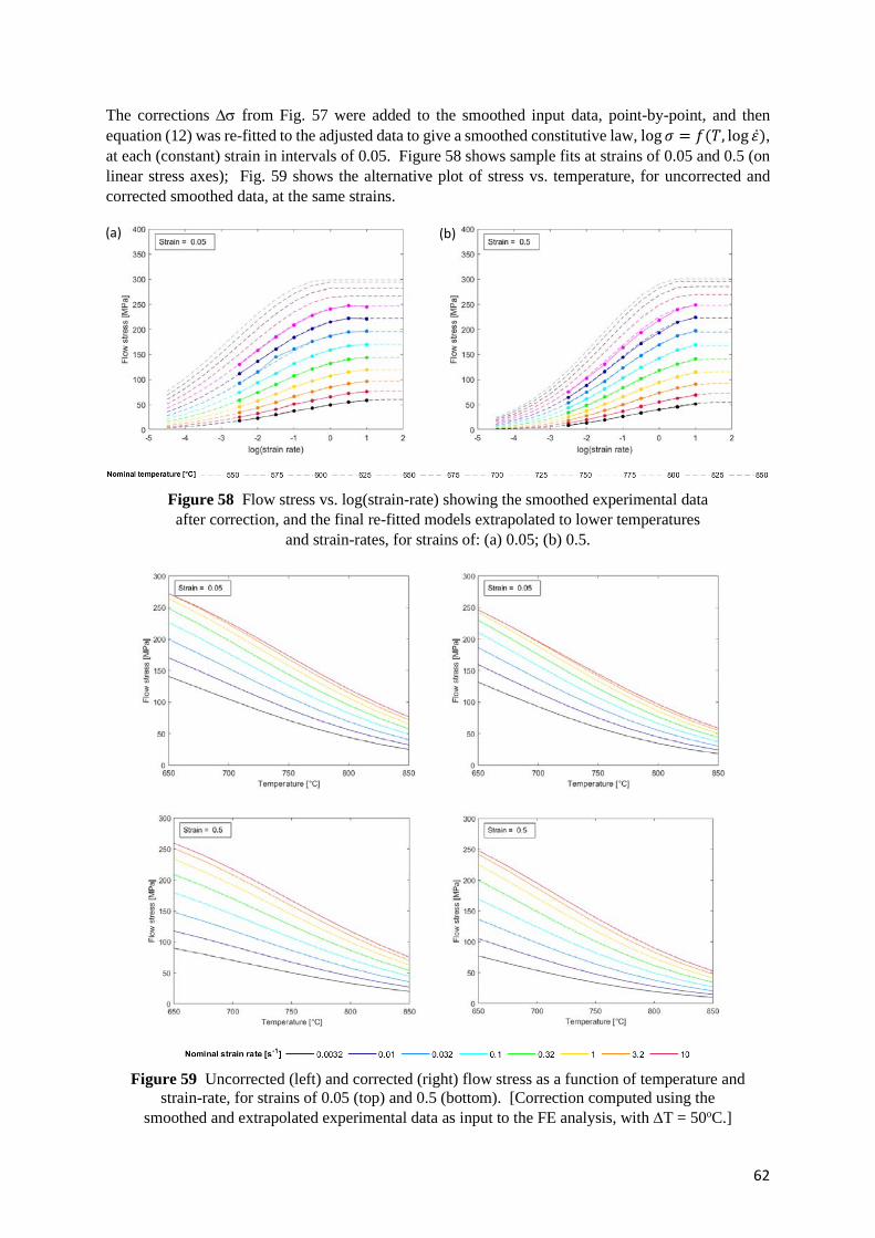
62

The corrections ∆σ from Fig. 57 were added to the smoothed input data, point-by-point, and then equation (12) was re-fitted to the adjusted data to give a smoothed constitutive law, log𝜎𝜎 = 𝑓𝑓(𝑇𝑇, log 𝜀𝜀̇), at each (constant) strain in intervals of 0.05. Figure 58 shows sample fits at strains of 0.05 and 0.5 (on linear stress axes); Fig. 59 shows the alternative plot of stress vs. temperature, for uncorrected and corrected smoothed data, at the same strains.

Figure 58 Flow stress vs. log(strain-rate) showing the smoothed experimental data after correction, and the final re-fitted models extrapolated to lower temperatures

and strain-rates, for strains of: (a) 0.05; (b) 0.5.

Figure 59 Uncorrected (left) and corrected (right) flow stress as a function of temperature and

strain-rate, for strains of 0.05 (top) and 0.5 (bottom). [Correction computed using the smoothed and extrapolated experimental data as input to the FE analysis, with ∆T = 50oC.]

(a) (b)

63

The broad appearance of the uncorrected and corrected curves is similar at each strain, but note that the absolute shifts in the curves are of the order of 10-30 MPa (Fig. 57), which is a significant fraction of the “notional” flow stress from the experiments. This formulation now avoids the extrapolation issues encountered previously, with the stress remaining positive for all strain-rates, strain and temperatures. The same quasi-static behaviours were imposed at very low and very high strain-rates, giving monotonically rising stress with decreasing temperature at all strain-rates, and providing numerical robustness for modest extrapolation upwards in strain-rate, or downwards in temperature, and down to zero strain-rate at the boundary of the dead metal zone.

To validate the final correction to the constitutive data, the same 3×3 matrix of conditions were re-predicted using the corrected flow stress – Fig. 60. In all cases the fit between prediction and experiment is good.

Figure 60 FE predicted stress-strain curves for the same 3×3 matrix of temperatures and strain-rates as Fig. 54. Solid red: smoothed experimental data (also used as initial input to FE to find the

correction); dashed red: corrected input to FE validation; dashed blue: resulting predicted output.

A more demanding test is to use the corrected data to re-predict the experiments combining the extreme values of temperature and strain-rate from the original 7×8 matrix of conditions – these are shown in Fig. 61. The fit is good at low strain-rates and at high temperatures, but begins to break down for the lowest temperature at the high strain rate of 10s-1. This is not surprising – these conditions were excluded from the original smoothing and fitting of the data, because these tests were at the limit of the capability of the dilatometer, with adiabatic heating increasing the temperature above the assumed nominal conditions. So agreement in this case is not expected.

0

50

100

150

200

250

300

Stre

ss [M

Pa]

0

50

100

150

200

250

300

Stre

ss [M

Pa]

0

50

100

150

200

250

300

0 0.2 0.4 0.6 0.8

Stre

ss [M

Pa]

Strain

0 0.2 0.4 0.6 0.8

Strain

0 0.2 0.4 0.6 0.8

Strain

0.01s-1 0.1s-1 1s-1

700°C

750°C

800°C

64

Figure 61 FE predicted stress-strain curves for a 2×2 matrix of the lowest and highest temperatures and strain-rates. Solid red: smoothed experimental data (also used as initial input to FE to find the correction); dashed red: corrected input to FE validation; dashed blue: resulting predicted output.

In summary, the piecewise correction of every individual test, followed by smoothing of the resulting data, gives the most robust outcome. Numerical stability is also maintained by assuming quasi-static (strain-rate independent) extrapolation of the log𝜎𝜎 = 𝑓𝑓(𝑇𝑇, log 𝜀𝜀̇) functions at very low strain-rates, and at higher rates from the point where the strain-rate sensitivity first falls to zero. The final stress-strain curves are now self-consistent with the experimental test data. The “best” corrected data are plotted as a set of stress-strain curves for all the experimental conditions in Fig. 62. There remain uncertainties in these curves however. due to the assumed (fixed) temperature gradient of 50oC, when it is known that the gradient will vary with test conditions, and with strain throughout a test. But the analysis has demonstrated the concept, and the same procedure is tested further in the follow-up study on Ti alloys [14], for which the temperature gradient in the sample is better characterised.

An aspect of the problem identified in this work is that the initial constitutive law needed to calculate the correction must extend to zero strain-rate in all cases (due to the dead metal zone). If the experimental dataset were more sparse, then extrapolation becomes much less reliable and it might prove impossible to calculate the correction with any confidence. In this case, an alternative set of input data must be used, provided this has a reasonably close 𝜎𝜎 = 𝑓𝑓(𝑇𝑇, 𝜀𝜀̇, 𝜀𝜀), i.e. published data for the same or a very similar alloy. This is the approach used in the subsequent work on hot compression of Ti alloys [14].

0

50

100

150

200

250

300St

ress

[MPa

]

0

50

100

150

200

250

300

0 0.2 0.4 0.6 0.8

Stre

ss [M

Pa]

Strain0 0.2 0.4 0.6 0.8

Strain

0.0032s-1 10s-1

650°C

850°C

65

Figure 62 Complete corrected stress-strain curves for full experimental test matrix.

66

7. Further applications of the FE model

Prediction of extent of barrelling

The corrected constitutive data may now be used to illustrate a number of potential outputs from the FE model. First, as an additional quantitative validation of the FE model, the predicted shape of the deformed sample can be compared with experiment. Sample cross-sections, such as that shown in Fig.3, often show a degree of asymmetry (both top to bottom, and from one side to the other). However, simple measures of barrelling can be made with calipers, without sectioning the sample. By measuring the length and assuming volume conservation, an average final diameter can be evaluated; then, by measuring the maximum diameter, a single measure of barrelling is obtained: the ratio of maximum to average diameter.

This ratio was calculated for all 144 experimental trials, and averaged for the two trials conducted at each of the 72 tested conditions. Figure 63 shows this ratio as a contour map of log(strain-rate ) against temperature – for the experimental data in Fig. 63(a), with the equivalent map derived from the predictions of the FE model in Fig. 63(b). Both maps show a similar trend, barrelling increasing from top left of the map to bottom right. The spread of values in the experiments is greater than predicted by the FE model – particularly the maximum ratio observed. This is consistent with asymmetry in the experimental tests leading to greater shape distortion, whereas the FE predictions remain perfectly axisymmetric.

Figure 63 Ratio of the maximum cross-section area to the average cross-section area, as a function of temperature and log(strain rate): (a) experimental data; (b) FE modelling results.

Prediction of extent of strain-rate sensitivity

A further application of the FE corrected flow stress data is to predict characteristics of the constitutive data, such as the strain-rate sensitivity, 𝑚𝑚 = 𝑑𝑑(log𝜎𝜎)/𝑑𝑑(log 𝜀𝜀̇). This parameter is commonly presented in the literature as a ‘processing map’, to guide choice of forming conditions in hot forging for example. Daniel et al. [1] demonstrate the issues that can be associated with the data handling used to generate such plots, ranging from the extent of the dataset, to the fitting function used before differentiating to find m. It was also pointed out that fitting to raw data without correcting for friction and inhomogeneous temperature would lead to errors. Figure 64 illustrates the changes in the map that can result from the last of these effects. The map in Fig. 64(b) is derived from cubic fits to the raw experimental data in Fig 64(a); Figs. 64(c,d) show the equivalent plots using the FE corrected and smoothed constitutive data. While the trend in strain-rate sensitivity is in broad agreement with temperature and strain-rate, the extreme values differ, and the smoothed, corrected data gives a cleaner set of contours. Figure 64(e,f) shows the corresponding map from a broader range of experimental temperatures [30]. Over the domain of the experiments in the current work, there are significant differences in the strain-rate

67

sensitivity, which have higher values here for all temperatures and strain-rates than in the published work.

Figure 64 (a,c,e) Flow stress data for 𝜀𝜀 = 0.5 with cubic fits (dashed lines), and (b.d.e) processing maps of strain-rate sensitivity m, derived from the cubic fits.

(a-b) uncorrected experimental data; (c-d) smoothed data corrected using the FE model; (e-f) data from Chakravartty et al. [30]

(e) (f)

(a) (b)

(c) (d)

68

Mapping of deformation conditions

The spatial deviation of the local deformation conditions, compared to the nominal values, is a central outcome of the FE analysis in this report. Another visualisation technique is proposed to indicate the spread of 𝑇𝑇 and 𝜀𝜀̇ conditions from the nominal value. Figure 65 shows contour maps of the von Mises equivalent plastic strain at the maximum compression, as a function of temperature and strain-rate for two temperature gradients, ∆T = 100°C and 50°C. These maps give an indication of the spread of deformation conditions (relative to nominal) over which significant strain occurs (with a lower limit of ε = 0.2). The peak contour value indicates the maximum strain, and hence its magnification compared to the notional true value of 0.69, as well as the conditions at the point of maximum strain (here, a higher strain-rate at the nominal temperature, since the mid-plane temperature is assumed to be constant). Since in the current work the temperature distribution is only an estimate, these maps should not be overinterpreted, but serves again as a proof of concept. The approach will be tested further in the subsequent work on Ti alloys [14], where the temperature distributions are time-dependent predictions of a full thermal model.

Figure 65 von Mises equivalent plastic strain as a function of temperature and strain-rate, for Tnominal = 750°C, 𝜀𝜀̇nominal = 0.1s-1 and 𝜀𝜀 = 0.69, with: (a) ∆T = 50°C; (b) ∆T = 100°C.

Nominal test conditions are indicated by a magenta circle.

Prediction of local deformation conditions

The FE model may also be used to track the history of the local deformation conditions at any point within the material cross-section, by following the temperature, strain-rate and strain at selected nodes in the FE mesh. Figure 66 shows sample histories of equivalent plastic strain and strain-rate, for a selected nominal temperature and stain-rate, at the centre of the sample, and at a point on the mid-plane initially located at half the radius from the centre. Compared to the nominal test conditions, the strain-rate at both locations is immediately a factor of two greater at both locations, and remains at this level or above at the centre, while off-axis the strain-rate progressively falls. These differences may be important in interpreting the evolution of microstructure throughout the sample, both in terms of average values and spatial variation – for example, if texture pole figures are evaluated from a significant fraction of the cross-section and associated with the nominal test conditions. Note that, as before, there is no temperature history to output in this case, since a constant mid-plane temperature is imposed. However, with a full thermal model of the test (as in the work on Ti alloys [14]) the full T(t) at each point could also be predicted, including the high strain-rate cases in which adiabatic heating increases the temperature above the nominal test value.

(a) (b)

69

Figure 66 FE predictions of deformation histories on the mid-plane of the sample, at the centre and a distance of half the radius, for Tnominal = 750°C, 𝜀𝜀̇nominal = 0.1s-1 (dashed line), ∆T = 50°C, and 𝜀𝜀 = 0.69.

(a) von Mises equivalent plastic strain; (b) von Mises equivalent plastic strain-rate.

8. Conclusions

A finite element model has been developed for a small-scale dilatometer rig used for hot compression testing of ZrNb alloy. The FE analysis enabled the true stress-strain curves to be corrected, allowing for barrelling due to friction at the workpiece-platen interface, and due to the temperature gradient between the mid-plane of the sample and the platen. In the current work, a fixed temperature gradient below the nominal test temperature was imposed, as a proof of concept. This will be refined in subsequent work on Ti alloys, in which the temperature gradient is better characterised.

An investigation of models containing multiple adjustable parameters, such as the Johnson-Cook equation, showed that the raw data could be fitted with reasonable accuracy to these functions. This however demonstrates the lack of physical validity in the fit, and the risks of over-fitting, since the raw data was as-yet uncorrected. The Sellars-Tegart (perfectly plastic) model could also be fitted with reasonable accuracy to the data at a low strain (5%), but the values found for physical parameters such as the activation energy were questionable, falling above the range expected from the literature. These investigations however did highlight that the high strain-rate, low temperature data were of questionable accuracy – a consequence of adiabatic heating increasing the temperature significantly above the nominal value.

In the present work, the requirement was to have a smoothed fit to the experimental data for 𝜎𝜎 =𝑓𝑓(𝑇𝑇, 𝜀𝜀̇, 𝜀𝜀), as the starting input data for the FE computation of the correction to the true stress due to inhomogeneous deformation. For the purposes of setting up the FE model, and testing its sensitivity to boundary conditions and mesh size, the Sellars-Tegart model was sufficient. But in order to compute the correction to the flow stress, it was necessary to include the strain-dependence. A novel approach was developed, using quadratic fits for log 𝜎𝜎 = 𝑓𝑓(𝑇𝑇, log 𝜀𝜀̇), at discrete strains in intervals of 0.05. This had the advantage of providing robust extrapolation beyond the domain of the experiments, notably down to zero strain-rate – a requirement in this context due to the presence of dead metal zones in the sample adjacent to the platens.

The methodology for correcting the flow stress was first trialled using only a 2×2 matrix of test temperatures and strain-rates, and fitting a planar surface to the resulting values of ∆𝜎𝜎 = 𝑓𝑓(𝑇𝑇, 𝜀𝜀̇) at the same discrete intervals in strain. This however led to non-physical extrapolation errors, particularly at low strain-rates and high temperatures, regardless of whether the Sellars-Tegart model or the smoothed experimental data were used as input. The solution was to calculate the correction over the full matrix

0

0.5

1

1.5

2

0 2 4 6 8

Von

Mis

es e

quiv

alen

t str

ain

Time [s]

Mid-plane, centreMid-plane, half-radiusNominal strain

(a)

0

0.1

0.2

0.3

0.4

0 2 4 6 8

Von

Mis

es e

quiv

alen

t str

ain

rate

Time [s]

Mid-plane, centreMid-plane, half-radiusNominal strain rate

(b)

70

of test conditions, and to apply these point-by-point to the original smoothed experimental data, re-fitting the resulting values to the same quadratic function for log 𝜎𝜎 = 𝑓𝑓(𝑇𝑇, log 𝜀𝜀̇) at each strain.

When the resulting corrected constitutive data was fed back into the FE model, the experimental “notional” stress-strain response (i.e. essentially the force-displacement response) could be predicted closely over the full matrix of test conditions. The only deviation occurred at the highest strain-rates at low temperatures, where the experimental data are questionable in any case (as noted above).

The application of the corrected data was illustrated for a number of purposes: (a) correlation with experimental measurements of barrelling; (b) prediction of strain-rate sensitivity, commonly presented as ‘processing maps’ n the literature; (c) visualisation of the spread of local deformation conditions in the sample, relative to the nominal temperature and strain-rate; and (d) prediction of local histories of strain and strain-rate at different locations within the sample (for use alongside interpretation of deformation microstructures).

It is not claimed that the resulting stress-strain curves provide a definitive constitutive response for the ZrNb alloy, since the correction applied depends on the temperature gradient, for which a constant value was imposed. But the analysis demonstrates that there is a significant influence of the inhomogeneity of deformation on the calculated true stress-strain response (and other outputs of the FE model). A more accurate correction requires a better knowledge of the temperature distribution in the sample throughout each test, requiring greater experimental instrumentation, and an associated heat flow model. This will be presented in future work on the same rig in Ti alloys [14].

References [1] C.S. Daniel, P. Jedrasiak, C.J. Peyton, J.Q. da Fonseca, H.R. Shercliff, L. Bradley, P.D. Honniball,

"Quantifying processing map uncertainties by modelling the hot compression behavior of a Zr-2.5Nb alloy," in 19th international symposium on zirconium in the nuclear industry, Manchester, 2019.

[2] C.K. Gupta, "Structural Materials: Niobium," in Materials in Nuclear Energy Applications, Volume II, Boca Raton, FL, CRC Press, 2018, pp. 20-27.

[3] C.R. Boer, N.M.R.S. Rebelo, H.A.B. Rydstad, G. Schröder, Process Modelling of Metal Forming and Thermomechanical Treatment, Heidelberg: Springer-Verlag, 1986.

[4] H.R. Shercliff, A.M. Lovatt, "Modelling of microstrucure evolution in hot deformation," Philosophical Transactions of the Royal Society A, vol. 357, pp. 1621-1643, 1999.

[5] P. Hartley, I. Pillinger, "Numerical simulation of the forging process," Computer Methods in Applied Mechanics and Engineering, vol. 195, no. 48–49, pp. 6676-6690, 2006.

[6] K. Runesson, Constitutive modeling of engineering materials - theory and computation, The Primer, 7th edition, Goteborg: Chalmers University of Technology, 2006.

[7] Y.C. Lin, X.M. Chen, "A critical review of experimental results and constitutive descriptions for metals and alloys in hot working," Materials and Design, vol. 32, no. 4, p. 1733–1759, 2011.

[8] Y. V. R. K. Prasad, T. Seshacharyulu, "Modelling of hot deformation for microstructural control," International Materials Reviews, vol. 43, no. 6, pp. 243-258, 1998.

[9] C. M. Sellars, "Modelling microstructural development during hot rolling," Materials Science and Technology, vol. 6, no. 11, pp. 1072-1081, 1990.

[10] C.S. Daniel, "An investigation into the texture development during hot-rolling of dual-phase zirconium alloys (Eng.D. thesis)," University of Manchester, Manchester, 2018.

[11] G.E. Dieter, H.A. Kuhn, S.L. Seminatin, editors, "Hot-Compression Testing," in Handbook of Workability and Process Design, Materials Park, OH, ASM International, 2003, pp. 61-67.

[12] TA Instruments, "DIL 805A/D/T," 04 06 2019. [Online]. Available: https://www.tainstruments.com/. [Accessed 04 06 2019].

71

[13] Y.C. Lin, M.S. Chen, J. Zhong, "Constitutive modeling for elevated temperature flow behavior of 42CrMo steel," Computational Materials Science, vol. 42, no. 3, pp. 470-477, 2008.

[14] P. Jedrasiak, H.R. Shercliff, "Modelling of thermal field and inhomogeneous deformation in hot compression of titanium alloys (unpublished work)".

[15] C. Peyton, "Generating and Evaluating the Strain Rate Sensitivity Processing Maps for Zr-2.5Nb (Thesis)," University of Manchester, Manchester, 2018.

[16] ASM Handbook Volume 2: Properties and Selection : Nonferrous Alloys and Special-Purpose Materials,10th Ed., ASM International, 1990.

[17] F. Cardarelli, Materials Handbook, 2nd Ed., London: Springer-Verlag, 2008.

[18] G.R. Johnson, W.H. Cook, "A constitutive model and data for metals subjected to large strains, high strain rates and high," Proceedings of the 7th International Symposium on Ballistics, p. 541–547, 1983.

[19] C.M. Sellars, W.J. McTegart, "On the mechanism of hot deformation," Acta Metallurgica, vol. 14, no. 9, pp. 1136-1138, 1966.

[20] S. Mandal, V. Rakesh, P.V. Sivaprasad, S.Venugopal, K.V. Kasiviswanathan, "Constitutive equations to predict high temperature flow stress in a Ti-modified austenitic stainless steel," Materials Science and Engineering: A, vol. 500, no. 1-2, pp. 114-121, 2009.

[21] G. Ji, F. Li, Q. Li, H. Li, Z. Li, "A comparative study on Arrhenius-type constitutive model and artificial neural network model to predict high-temperature deformation behaviour in Aermet 100 steel," Materials Science and Engineering: A, vol. 528, no. 13-14, pp. 4774-4782, 2011.

[22] Y.C. Lin, Y.C. Xia, X.M. Chen, M.S. Chen, "Constitutive descriptions for hot compressed 2124-T851 aluminum alloy over a wide range of temperature and strain rate," Computational Materials Science, vol. 50, no. 1, pp. 227-233, 2010.

[23] C. Liao, H. Wu, S. Lee, F. Zhu, H. Liu, C. Wu, "Strain-dependent constitutive analysis of extruded AZ61 Mg alloy under hot compression," Materials Science and Engineering: A, vol. 565, pp. 1-8, 2013.

[24] P. Geng, G. Qin, J. Zhou, Z. Zou, "Hot deformation behavior and constitutive model of GH4169 superalloy for linear friction welding process," Journal of Manufacturing Processes, vol. 32, pp. 469-481, 2018.

[25] C. Herzig, U. Kohler, S.V. Divinski, "Tracer diffusion and mechanism of nonArrhenius diffusion behavior of Zr and Nb in body-centered cubic Zr–Nb alloys," Journal of Applied Physics, vol. 85, no. 12, pp. 8119-8130, 1999.

[26] H.J. Frost, M.F. Ashby , Deformation-mechanism Maps: The Plasticity and Creep of Metals and Ceramics, Oxford: Pergamon Press, 1982.

[27] M. Smith, "Mechanical contact properties," in Abaqus Analysis User's Guide, Version 6.9, Providence, RI, Simulia, 2009.

[28] M. Smith, "Contact pressure-overclosure relationships," in Abaqus Analysis User's Guide, Version 6.9, Providence, RI, Simulia, 2009.

[29] P. Hartley, C.E.N. Sturgess, G.W. Rowe, "Influence of friction on the prediction of forces, pressure distributions and properties in upset forging," International Journal of Mechanical Sciences, vol. 22, no. 12, pp. 743-753, 1980.

[30] J. K. Chakravartty, R. Kapoor, A. Sarkar, V. Kumar, S. K. Jha, N. Saibaba, S. Banerjee, "Identification of Safe Hot-Working Conditions in Cast Zr-2.5Nb," in Zirconium in the Nuclear Industry: 17th Volume, ed. B. Comstock and P. Barberis, West Conshohocken, PA, ASTM International, 2015, p. 259–281.