d130.13 final dissemination - cordis · d130.13 final dissemination version 1.0 / public document /...
TRANSCRIPT

Safe and Efficient Electrical Vehicle
7th Framework programme / FP7-2010-ICT-GC /
ICT for the fully electrical vehicle / Grant Agreement Number 258133
D130.13 Final Dissemination

D130.13 Final dissemination
Version 1.0 / Public Document / 07.10.2013 page 2
Aデエラヴゲ
Name Company
GLASER, Sébastien IFSTTAR
RWキゲキラミ Iエ;ヴデ
Version Date Reason
0.1 18.09.2013 Basis document
0.2, 0.3 7.10.2013 Website, brochure, attached papers
added
1.0 7.10.2013 Final formatting, released version
Copyright, eFuture Consortium, 2011

D130.13 Final dissemination
Version 1.0 / Public Document / 07.10.2013 page 3
EWIデキW Sママ;ヴ
This deliverable covers the dissemination activities in the frame of the eFuture project. For the
scientific dissemination, the project team was very productive:
More than 25 papers were presented at national and international conferences
3 papers were published in technical or scientific journals
The full project was presented at several workshop and the team will attend at least at
ICT 2013 conference and will present the results at a stand promoted by the European
Commission.
The dissemination also includes the promotion of the project to a wider audience. A brochure is
now available and presents the achievements of the project.
The document will be updated per 30.11.2013 by dissemination activities in November 2013.

D130.13 Final dissemination
Version 1.0 / Public Document / 07.10.2013 page 4
T;HノW ラa CラミデWミデ
1 Scientific Dissemination .................................................................................................... 5
1.3 2013 .................................................................................................................................... 5
1.4 2012 .................................................................................................................................... 6
1.5 2011 .................................................................................................................................... 7
2 General presentation ........................................................................................................ 8
2.1 Website and logo ................................................................................................................ 8
2.2 Project presentation ........................................................................................................... 9
2.3 Brochure .............................................................................................................................. 9
3 Appendix ........................................................................................................................ 10
D130.13 Final dissemination
Version 1.0 / Public Document / 07.10.2013 page 5
1 SIキWミデキaキI DキゲゲWマキミ;デキラミ
For the scientific dissemination, the project team was very productive:
More than 25 papers were presented at national and international conferences
3 papers were published in technical or scientific journals
The full project was presented at several workshop and the team will attend at least at
ICT 2013 conference and will present the results at a stand promoted by the European
Commission.
In the annex, you will find some articles that present the work of the team.
1.3 2013
1. Köhler U.; Decius N.; Masjosthusmann, C.; Büker U. "Development of a scalable multi-
controller ECU for a smart, safe and efficient Battery Electric Vehicle " AMAA 2013, Berlin
2. Masjosthusmann, C.; Kohler, U.; Decius, N.; Buker U." Ein Verhaltensmodell und ein
Laborprüfstand zur SiL- und HiL-Simulation eines zentralen Steuergeräts für ein
intelligent-effizientes Elektrofahrzeug", ASIM Workshop 2013
3. Masjosthusmann, C. ; Buker U.; Kohler, U.; Decius, N., "A Load Balancing Strategy for
Increasing Battery Lifetime in Electric Vehicles" SAE Technical Paper 2013-01-0499
4. Rittger, L.; Schmitz, M. "The compatibility of energy efficiency with pleasure of driving"
55th Conference of Experimental Psychologists (TeaP), Vienna, 25.-27.03.2013.
5. Rittger, L.; Schmitz, M. "The compatibility of energy efficiency with pleasure of driving"
ICDBT 2013, Helsinki (Finland)
6. Korte M.; Kaiser G.; Holzmann F.; Roth H. " Design of a Robust Adaptive Vehicle Observer
Towards Delayed and Missing Vehicle Dynamics Sensor Signals by Usage of Markov
Chains" American Control Conference 2013
7. Korte M.; Kaiser G.; Roth H. " Robust Vehicle Observer to Enhance Torque Vectoring in an
EV", Autoreg 2013
8. Glaser S.; Orfila O.; Nouveliere L.; Potarusov R.; Akhegaonkar S.; Holzmann F.; Scheuch V.
" Smart and Green ACC, adaptation of the ACC strategy for electric vehicle with
regenerative capacity", IEEE IV Symposium 2013
9. Glaser S.; Akhegaonkar S.; Orfila O.; Nouveliere L.; Scheuch V.; Holzmann F. "Smart And
Green ACC, Safety and efficiency for a longitudinal driving assistance" AMAA 2013, Berlin
10. Glaser S.; Orfila O.; Potarusov R.; Nouveliere L. "Speed profile optimization for electric
vehicle with regenerative capacity" FAST zero 2013, Nagoya Japan
11. Schmitz M.; Jagiellowicz M.; Maag C.; Hanig M. "Impact of a combined acceleratorにbrake
pedal solution on efficient driving." IET Intelligent Transport Systems に Special Issue:
Human-Centred Design for Intelligent Transport Systems, 7(2), 203 に 209.
12. Rittger, L.; Schmitz, M. "The Compatibility of Energy Efficiency with Pleasure of Driving in
a Fully Electric Vehicle." In L. Dorn & M. Sullman (Eds.), Driver Behaviour and
TrainingVolume VI (pp. 207-222). Surrey: Ashgate Publishing.
13. Revilloud M.; Gruyer D.; Pollard E. " An improved approach for robust road marking
detection and tracking applied to multi-lane estimation.", IEEE IV Symposium 2013

D130.13 Final dissemination
Version 1.0 / Public Document / 07.10.2013 page 6
14. FakhFakh N., Gruyer D.; Aubert D. " Weighted V-disparity Approach for Obstacles
Localization in Highway Environments", IEEE IV Symposium 2013
15. Scheuch V.; Kaiser G.; Korte M.; Grabs P.; Kreft F.; Holzmann F. "A safe torque vectoring
function for an electric vehicle", EVS27 Symposium, Barcelona Spain 2013
1.4 2012
1. Schmitz M.; Jagiellowicz M.; Maag C.; Hanig M. "The impact of different pedal solutions
for supporting efficient driving with electric vehicles." In P. V. Mora, J.-F. Pace & L.
Mendoza (Hrsg.), Proceedings of European Conference on Human Centered Design for
Intelligent Transport Systems (S. 21-28). Valencia: HUMANIST.
2. Schmitz M.; Jagiellowicz M.; Maag C.; Hanig M. "Drivers´ acceptance of limiting vehicle
dynamics in electric vehicles." ICTTP 2012, Groningen, 28.08.-31.08.2012.
3. Glaser S.; Orfila, O.; Schmaeche M. "Safety of a torque vectoring LKAS on an in-wheel
motor electric vehicle", EEVC 2012, Bruxelles, Belgium
4. Scheuch V.; Kaiser G.; Holzmann F., "Eine innovative Funktionsarchitektur für das
Elektrofahrzeug, Ulrich Brill", expert Verlag, Renningen, 2012
5. Jagiellowicz M.; Schmitz M.; Maag C.; Hanig M. "The impact of a combined pedal solution
on efficient electric driving and drivers´ acceptance: A driving simulator study". 54.
Tagung experimentell arbeitender Psychologen (TeaP), Mannheim, 01.04.-04.04.2012.
6. Schmitz M.; Jagiellowicz M.; Maag C.; Hanig M., "Drivers´ acceptance of limiting vehicle
dynamics in electric vehicles." 54. Tagung experimentell arbeitender Psychologen (TeaP),
Mannheim, 01.04.-04.04.2012.
7. Masjosthusmann, C.; Kohler, U.; Decius, N.; Buker, U., "A vehicle energy management
system for a Battery Electric Vehicle," Vehicle Power and Propulsion Conference (VPPC),
2012 IEEE , vol., no., pp.339,344, 9-12 Oct. 2012
8. Akhegaonkar S.; Nouvelière L.: Potarusov R.; Scheuch V.; Holzmann F.; Glaser S.
"Modeling and Simulation of Battery Electric Vehicle to Develop an Energy Optimization
Algorithm", AVEC 2012, Seoul, Korea
9. Korte M.; Kaiser G.; Holzmann F.; Scheuch V.; Roth H. "Design of a robust plausibility
check for an adaptive vehicle observer in an electric vehicle", 16th International Forum on
Advanced Microsystems for Automotive Applications, 30-31 May 2012, Berlin, Germany
10. Scheuch V.; Kaiser G.; Holzmann F.; Glaser S. "Simplified architecture by the use of
decision units" 16th International Forum on Advanced Microsystems for Automotive
Applications, 30-31 May 2012, Berlin, Germany
11. Scheuch V.; Kaiser G.; Straschill R.; Holzmann F.; " A new functional architecture for the
improvement of eCar efficiency and safety", 21st Aachen Colloquium Automobile and
Engine Technology 2012

D130.13 Final dissemination
Version 1.0 / Public Document / 07.10.2013 page 7
1.5 2011
1. Kaiser, G. ; Holzmann, F. ; Chretien, B. ; Korte, M. ; Werner, H. "Torque Vectoring with a
feedback and feed forward controller - applied to a through the road hybrid electric
vehicle" Intelligent Vehicles Symposium (IV), 2011 IEEE, Publication Year: 2011 , Page(s):
448 - 453
2. Korte M.; Holzmann F.: Scheuch V.; Roth H. "Development of an adaptive vehicle observer
for an electric vehicle", EEVC Brussels, Belgium, October 26-28, 2011
3. Scheuch V. "E/E architecture for electric vehicle" ATZ Elektronik, 2011 に 06 (see online
www.atzonline.de)

D130.13 Final dissemination
Version 1.0 / Public Document / 07.10.2013 page 8
2 GWミWヴ;ノ ヮヴWゲWミデ;デキラミ
Verdure was selected at the beginning of the project to handle most of the non-scientific
dissemination, providing the logo, the website and the final brochure. Partners also promote the
full project at several events.
2.1 Website and logo
After an internal poll, the logo was selected during the first steering committee. It is presented
here.
The website allows a dissemination during the whole project duration, it will be maintained after
the project end.
D130.13 Final dissemination
Version 1.0 / Public Document / 07.10.2013 page 9
2.2 Project presentation
1. June 2011, INTEDIS, "eFuture に General project overview", Third Workshop on Research
for the fully electric vehicle, Bruxelles, Belgium
2. June 2011, INTEDIS " eFuture に General project overview" Joint EC / EPoSS / ERTRAC
Expert Workshop 2011, Berlin, Germany
3. June 2013, TMETC, WMG Academy trainer
4. November 2013 , All partners, "Efuture - project presentation", ICT 2013, Vilnius, Lituanie
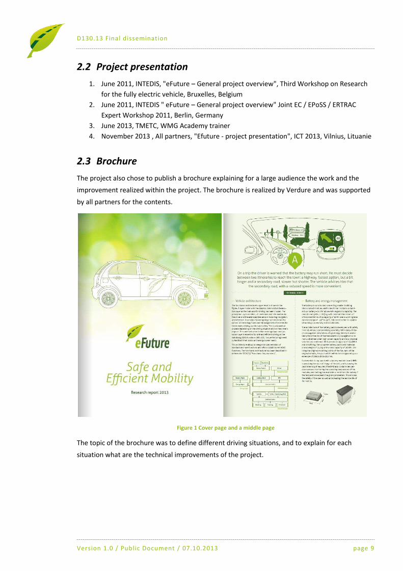
2.3 Brochure
The project also chose to publish a brochure explaining for a large audience the work and the
improvement realized within the project. The brochure is realized by Verdure and was supported
by all partners for the contents.
Figure 1 Cover page and a middle page
The topic of the brochure was to define different driving situations, and to explain for each
situation what are the technical improvements of the project.

D130.13 Final dissemination
Version 1.0 / Public Document / 07.10.2013 page 10
3 AヮヮWミSキ
For orientation on the public and scientific articles, we present some selected papers in the
appendix of this deliverable:
1. Scheuch V. "E/E architecture for electric vehicle" ATZ Elektronik, 2011 に 06 (see online
www.atzonline.de)
2. Glaser S.; Akhegaonkar S.; Orfila O.; Nouveliere L.; Scheuch V.; Holzmann F. "Smart And
Green ACC, Safety and efficiency for a longitudinal driving assistance" AMAA 2013, Berlin
3. Revilloud M.; Gruyer D.; Pollard E. " An improved approach for robust road marking detection
and tracking applied to multi-lane estimation.", IEEE IV Symposium 2013
4. FakhFakh N., Gruyer D.; Aubert D. " Weighted V-disparity Approach for Obstacles Localization
in Highway Environments", IEEE IV Symposium 2013
5. Rittger, L.; Schmitz, M. "The compatibility of energy efficiency with pleasure of driving" 55th
Conference of Experimental Psychologists (TeaP), Vienna, 25.-27.03.2013.
6. Schmitz M.; Jagiellowicz M.; Maag C.; Hanig M. "The impact of different pedal solutions for
supporting efficient driving with electric vehicles." In P. V. Mora, J.-F. Pace & L. Mendoza
(Hrsg.), Proceedings of European Conference on Human Centered Design for Intelligent
Transport Systems (S. 21-28). Valencia: HUMANIST.
7. Scheuch V.; Kaiser G.; Korte M.; Grabs P.; Kreft F.; Holzmann F. "A safe torque vectoring
function for an electric vehicle", EVS27 Symposium, Barcelona Spain 2013

E/E-ARCHITEKTUR FÜR
BATTERIE-ELEKTRISCHE FAHRZEUGE
In einem europäischen Forschungsprojekt namens eFuture untersucht Intedis gemeinsam mit fünf
weiteren Partnern aus vier Ländern neue Funktionen für das Elektromobil, die in eine schlanke
E / E-Architektur gebettet sind. Diese soll die zunehmende Komplexität beherrschbar machen und
für eine sichere Ansteuerung von Aktuatoren (Motoren, Bremse und Lenkung) sorgen.
INDUSTRIE E/E-ARCHITEKTUR
28

ZIELE DES GESAMTPROJEKTS
Das Forschungsprojekt eFuture [1] widmet sich der Reichweiten
optimierung und Fahrsicherheit von Elektrofahrzeugen. Zwei An
sätze verfolgen die fünf Partner der Intedis, Tata, Hella, Miljøbil
Grenland, IFSTTAR (Französisches Forschungsinstitut für Trans
port, Straßenbau und Netze) und WIVW (Würzburger Institut für
Verkehrswissenschaften):
: Der Energiehaushalt des Fahrzeugs soll optimiert werden,
indem Entscheidungsmodule in einer neu strukturierten E/E
Architektur zwischen den Bereichen Komfort, Sicherheit und
Effizienz vermitteln. Zum anderen wird der Fahrer durch Emp
fehlungen, Hinweise und Assistenzsysteme in die Reichweiten
optimierung einbezogen.
: Die Fahrsicherheit von Elektrofahrzeugen mit mehr als einem
Antriebsmotor soll erhöht werden. Um Gefahrensituationen
durch nichtsynchrone Radansteuerung zu vermeiden, ist eine
Synchronisierung der Steuerungen notwendige, welche ein
intelligentes Software und Sicherheitskonzept erfordert.
Das Konsortium bedient sich dazu der klassischen Werkzeuge
Konzeptentwicklung, numerische Simulation und Validierung im
Fahrzeugversuch. Nach der ersten Phase der Architekturdefini
tion, die bereits abgeschlossen ist, werden in der zweiten Phase
die Komponenten und das Gesamtfahrzeug aufgebaut. Die dritte
Phase beinhaltet die Optimierung und Validierung der Funktionen
und Algorithmen im Gesamtfahrzeugversuch.
Dieser Artikel konzentriert sich auf die Reichweitenoptimierung,
speziell die E/EArchitektur, die die Basis für mehr Effizienz bildet.
Mit Hilfe von zentralen Entscheidungseinheiten (Decision Units),
gelingt eine Priorisierung von Anforderungen an den Antriebs
strang, die je nach Fahrzustand den Komfort oder die Effizienz
begünstigt, jedoch eine hohe Fahrsicherheit immer gewährleistet.
E/E-ARCHITEKTUR
Die E/EArchitektur eines Fahrzeugs teilt sich in die Funktionsar
chitektur und die physikalische Architektur. Letztere umfasst die
Gesamtheit der Steuergeräte, die Netzwerk und die Kabelbaum
topologie, also die Hardware zur Verteilung von Energie und Sig
nalen. Um diese Netze bedarfsgerecht und schlank zu halten, ist
zunächst eine Analyse der gewünschten Fahrzeugfunktionen un
erlässlich, denn diese benötigen Sensoren, Aktuatoren, Informa
tionsaustausch mit anderen Funktionen, eine Energieversorgung
und ein Steuergerät, auf dem der Algorithmus eingebettet ist. Mit
der detaillierten Kenntnis aller Funktionen lässt sich eine Funk
tionsarchitektur erstellen, die die spezifischen Randbedingungen
des Fahrzeugs berücksichtigt. Dies sind im Falle des eFuturePro
jekts die maximale Energieeffizienz bei höchster Fahrsicherheit.
Die oberste Ebene der Funktionsarchitektur zeigt ❶. Es wurde
ein Lagenmodell gewählt, in dem die klassischen Lagen „Com
mand Layer“ und „Execution Layer“ die Hauptachse für den Fahr
betrieb darstellen. Der „Perception Layer“ vereint alle Umgebungs
informationen über den Fahrer und die Umgebungssensoren inklu
sive Navigation und eHorizon [2]. Parallel dient der „Energy Layer“
der Steuerung der Energieflüsse und der Zuteilung von Energiere
serven an die einzelnen Domänen Fahren, Komfort und Sicherheit.
Dies geschieht dynamisch, das heißt in Kenntnis und Abhängigkeit
der Fahrsituation und des Fahrerwunsches. Da die Fahrsicherheit
DR. VOLKER SCHEUCH
leitet das Projekt eFuture
bei der Intedis GmbH & Co. KG
in Würzburg.
AUTOR
2906I2011 6. Jahrgang

durch Funktionen wie ESC, ABS oder
Torque Vectoring realisiert werden, ist eine
Kommunikation mit dem „Command
Layer“ und dem „Exe cution Layer“
unerlässlich.
Um die Funktionskomplexität zu be
herrschen, verfolgt Intedis das Konzept de
zidierter Entscheidungsmodule (Decision
Units), die als Zustandsmaschinen (State
Machines) ausgeführt sind und gewisser
maßen als Zentralintelligenz des Funkti
onskonzepts dienen. Die Entscheidungs
module nehmen die Anforderungen oder
Randbedingungen der vorgelagerten Funk
tionen auf und entscheiden aufgrund defi
nierter Kriterien, welche Aktion in dieser
Situation durchzuführen ist. Beispielsweise
werden während einer Autobahnfahrt ver
schiedene Anforderungen an das Fahrzeug
gestellt: Das adaptive Geschwindigkeitsre
gelsystem (Adaptive Cruise Control – ACC)
möchte aufgrund einer Annäherung an
das vorausfahrende Fahrzeug abbremsen,
während der Fahrer jedoch durch eine
Lenkbewegung zu verstehen gibt, dass er
überholen möchte. Falls der Blinker nicht
betätigt wurde, würde der Spurhalteassis
tent (Lane Keeping Assistant – LKAS) mit
einem Gegenlenken antworten, das bei
gleichzeitigem Bremsen des ACC zu nicht
gewünschten Änderungen der Trajektorien
oder sogar der Fahrstabilität führen könnte.
Im Falle von einzeln operierenden
Funktionen können widersprechende
Aktionen nur vermieden werden, indem
jede Funktion eine entsprechende Situa
tionsabfrage mit einer Entscheidungs
logik beinhaltet. Die Decision Unit stellt
dies als Zentralfunktion allen aufrufen
den Funktionen zur Verfügung, sodass
diese eine schlankere Struktur bekommen
können und sich somit auch die Taktzeit
reduziert.
Das obige Beispiel lässt noch einen
V orteil des Konzepts erkennen. Der Über
gang zwischen verschiedenen Assistenz
funktionen beziehungsweise Fahrzustän
den ist durch einfache Regeln möglich.
Das Verhalten im Grenzbereich zwischen
Lateral und Longitudinaldynamik kann
individuell abgestimmt werden, sodass
widersprüchliche und gefährliche Aktio
nen von verschiedenen Funktionen ver
mieden werden. Das Gleiche gilt für den
Übergang von automatisiertem zu manuel
lem Fahren, in dem Unstetigkeiten zu uner
wünschtem Fahrverhalten führen können.
Die Entscheidung der Decision Unit
wird im Normalfall, in dem das Fahrzeug
sich in einem stabilen Fahrzustand befin
det, im Sinne einer effizienten Fahrweise
ge troffen. Solange weder der Fahrerwunsch
noch die Fahrsicherheit dagegen sprechen,
wird immer der für die ReichweitenMaxi
mierung günstigste Zustand angestrebt
(„grüne“ Fahrweise). Dieses Prinzip wird
durch die Nutzung der zentralen Entschei
dung begünstigt, da es keine parallelen
Funktionswege gibt.
Um die Komplexität der Decision Unit
zu reduzieren, wird diese Zentralfunktion
auf den Command Layer und den Exe
cution Layer verteilt. Die Decision Unit 1
im Command Layer ist für die Vermitt
lung zwischen den spurführenden Fah
rerassistenzen (ACC, LKAS, Notbrems
assistent), dem Fahrer und den Rand
bedingungen des Energiemanagement
verantwortlich. Die Entscheidung, wel
cher Trajektorie zu folgen ist, wird der
Decision Unit 2 im Execution Layer mit
geteilt. Diese prüft die Anforderung an die
Elektromotoren (Beschleunigen versus
Rekuperieren), die hydraulischen Bremsen
und die Lenkung gegen den aktuellen
Fahrzustand und extrapoliert die mögli
chen Auswirkungen dieses Manövers.
Falls es etwa zu einem Übersteuern käme,
würde die Decision Unit die Fahrregelung
an das ESC übergeben.
❶ Funktionsarchitektur des
eFuture-Fahrzeugs; ADAS
steht für Advanced Driver
Assistance Systems (erwei terte
Fahrerassistenzsysteme),
MMI ist die Abkürzung für
Mensch-Maschine-Interface
❷ Die intelligente Tempomatfunktion hilft durch Kenntnis des Straßenverlaufs, die Geschwindigkeit
anzupassen und gleichzeitig sicher und sparsam zu navigieren
INDUSTRIE E/E-ARCHITEKTUR
30
Das Konzept unterstützt außerdem die
Auslegung der Funktionsarchitektur hin
sichtlich der Anforderungen an die Funk
tionale Sicherheit (ISO 26262). Die sicher
heitskritischen Funktionen lassen sich auf
die Decision Units beschränken, indem
Plausibilitäts und Sicherheitsprüfungen
eingebaut werden, die keine fehlerhaften
Funktionsaufrufe zulassen (SafetyShell
Konzept).
NEUE FUNKTIONEN UNTERSTÜTZEN
EFFIZIENZ UND SICHERHEIT
Die Idee von eFuture ist es, etablierte
Funktionen zu nutzen, um neue Funkti o
nalitäten zu erreichen, ohne zusätzliche
Hardware zu integrieren. Dabei soll der
Begriff „Neu“ eher im Sinne der erstmaligen
Anwendung in einem Elektrofahrzeug
verstanden werden, da es sich meist um
bekannte, aber wenig verbreitete Funk ti
onen handelt. Die Integration neuer Funk
tionen hat außerdem den Vorteil, dass die
Architektur, also die logische und techni
sche Auslegung der Steuergeräte und
Netzwerke, auch offen ist für künftige
Innovationen. Denn der Anspruch von
eFuture ist es, eine zukunftsfähige und
erweiterbare Architektur für das Elektro
fahrzeug zu schaffen. Neben den bereits
beschriebenen „Entscheidungseinheiten“
als Zentralfunkti onen umfassen die neuen
Funktionen die Themenbereiche:
: Fahrstabilität: Das eFutureFahrzeug
konzept sieht einen DoppelmotorFront
antrieb vor, sodass per se ein elektro
nisches Differenzial notwendig ist. Die
Möglichkeit der unabhängigen Dreh
momomentverteilung auf die Front räder
wird als TorqueVectoringFunktion auch
zur Erhöhung der Fahrstabilität auf Fahr
bahnen mit lateral unterschiedlicher Rei
fenhaftung oder in Kurven ge nutzt.
: Durch eHorizon erhält der Fahrer „vor
ausschauende“ Informationen, die es
ihm ermöglichen, sein Fahrverhalten
optimal an die Verkehrssituationen
anzupassen. Auch die Assistenzsysteme
nutzen diese Informationen für einen
effizienten Umgang von Beschleunigen
und Rekuperieren. Somit lassen sich
kritische beziehungsweise ineffiziente
Manöver von vornherein vermeiden [3].
: Reichweitenmanagement: im Sinne
eines erweiterten, effizienzsteigernden
Energiemanagements mit Hilfe von
Assistenzsystemen.
REICHWEITENMANAGEMENT
Der Begriff Reichweitenmanagement
bekommt in Verbindung mit den knappen
Energieressourcen (begrenzter Aktionsra
dius) in einem Elektrofahrzeug eine
übergeordnete Bedeutung. Reichweiten
management soll den Fahrer dabei unter
stützen, den Zielort möglichst energie
sparend zu erreichen, oder sich ldurch
Fahhinweise eiten zu lassen, um so weit
wie möglich mit einer Batterieladung
beziehungsweise mit von vorab geplan
ten Zwischenladungen fahren zu kön
nen. Drei Aspekte werden im Reichwei
tenmanagement genutzt:
: Fahrerassistenz: Die Verschmelzung des
Abstandsregeltempomats (ACC) mit der
eHorizonFunktion. Wenn man Daten
wie Tempolimits, Steigungen, Kurven
radien, Verzweigungen, Einmündungen
für die ACCFunktion nutzt, lässt sich
zur Erhöhung der Fahrsicherheit die
SollGeschwindigkeit an die Fahrsitu
ation anpassen, ❷. In Verbindung mit
einem EcoModus lässt sich auch im
ACCBetrieb Energie sparen, indem vor
ausschauend die Geschwindigkeit redu
3106I2011 6. Jahrgang

ziert wird oder auf Beschleunigen ver
zichtet wird, sofern der Straßenverlauf
dies nahelegt, ❸.
: FahrerCoaching: Im eFutureFahrzeug
wird der Fahrer in den Regelkreis
einbezogen. Er erhält Hinweise zur
optimalen Rekuperation oder zum
Beschleunigungs verhalten und lernt
effizientes Fahren, so fern er die
auch abschaltbaren Funktionen nutzt.
Schließlich wird dem Fahrer signali
siert, ob sein Fahrtziel mit den vor
handenen Ressourcen und der der zei
tigen Effizienz erreichbar ist, ❹.
: Energiemanagement.
ENERGIEMANAGEMENT
Ein zentrales und vernetztes Energie
managementsystem (EMS) sorgt für
einen ausgewogenen und bedarfsge
rechten Energiefluss zwischen Hochvolt
Batterie und Verbrauchern. Das Projekt
eFuture nimmt neueste Erkenntnisse von
Batteriemanagementsystemen (BMS)
auf, die zur Genüge veröffentlicht worden
sind. Neu ist die Integration der beschrie
benen Priorisierungen „Sicherheit/Effi
zienz/Komfort“. Hier kommt zudem das
Verhalten des Fahrers ins Spiel, das eben
falls im Sinne des Energiemanagements
vom FahrerCoaching beeinflusst werden
kann: Eine präzise und detaillierte Ver
❸ Die neue Funktion des eHorizon erlaubt es, unnötiges Beschleunigen zu vermeiden,
falls der Straßenverlauf dies nahelegt
Weitere Informationen erhalten Sie unter: [email protected]
www.cd-adapco.com/battery
„CD-adapco entwickelt zur Zeit eine umfassende Lösung zur Modellierung von
Batterien innerhalb von STAR-CCM+.
Es ist ein Vergnügen gemeinsam mit CD-adapco an diesem Projekt zu arbeiten.”
RobeRt Spotnitz, pReSident - batteRy deSign LLC
STAR-CCM+: Lösungen für die BatteriemodellierungVollständig integrierte Strömungs- und Wärmesimulation vom einfachen Schaltkreis bis hin
zur kompletten Elektrochemie für Lithium-Ionen-Zellen, Packs und Fahrzeuginstallationen.
LITHIUM-IONEN-BATTERIE-SIMULATION MIT STAR-CCM+: POWER WITH EASE.
Cd-adapco ist der führende anbieter der gesamten bandbreite technischer Simulationslösungen
(Cae) für Strömung, Wärmeübergang und Struktur.
INDUSTRIE E/E-ARCHITEKTUR

READ THE ENGLISH E-MAGAZINE
order your test issue now:
DOWNLOAD DES BEITRAGS
www.ATZonline.de
brauchsberechnung und Reichweitenab
schätzung liefert dem Fahrer wertvolle
Informationen, um den eigenen Fahrstil
zu optimieren und um sein Vertrauen in
die Zuverlässigkeit des Elektrofahrzeugs
zu steigern. Das EMS ist auch gefragt,
falls die Leistungs fähigkeit der Hochvolt
batterie kurzfristig droht, überschritten
zu werden. Es kann die Entladeströme
dann zu Lasten niedrig priorisierter Ver
braucher wie Heizung oder Klimaanlage
reduzieren. Durch die Kopplung des
EMS mit der eHorizonFunktion kann
es prä zisere Aussagen über die Reich
weite treffen, da es Informationen über
die geplante Strecke, wie zum Beispiel
das Höhen und Geschwindigkeitsprofil,
mit einbeziehen kann.
Die beschriebenen Funktionen wurden
gemeinsam mit den konventionellen
Funktionen in einem numerischen
Si mulationsmodell dargestellt, sodass
Analyse und Optimierung einzeln sowie
im Verbund bereits virtuell stattfinden
können, bevor im letzten Teil von eFuture
die finale Kalib rierung im Realfahrzeug
vollzogen wird.
AUSBLICK
Der nächste Schritt im Projekt ist der
Aufbau des Konzepts als fahrfähiger
Prototyp. Dazu sind zunächst noch
Simulationsstudien notwendig, die das
Zusammenspiel der Funktionen in der
FahrerFahrzeugRegelschleife optimie
ren („FunctionintheLoop“). Nach
der vir tuellen Freigabe werden die Steu
ergeräte mit den Funkti onen program
miert und das Fahrzeug kann beweisen,
dass die Konzepte im Fahrversuch hal
ten, was sie auf dem Papier versprechen:
den Widerspruch zwischen Effizienz,
Komfort und Sicherheit aufzulösen helfen.
Das eFutureKonsortium möchte damit
einen weiteren Anstoß geben, das Elektro
fahrzeug künftig anders zu defi nieren als
konventionelle Fahrzeuge, und so einen
Beitrag zur effizienten Elektro mobilität
leisten.
LITERATURHINWEISE
[1] www.efuture-eu.org, gefördert durch die
Europäische Kommission unter der Fördernummer
258133
[2] Ress, C.; Etemad, A.; Kuck, D.; Boerger, M.:
Electronic Horizon – Supporting ADAS applications
with predictive map data. Cebit Papers 2006
[3] Kaiser, G.; Holzmann, F.; Chretien, B.; Korte,
M.; Werner, H.: Torque Vectoring with a feedback
and feed forward controller – applied to a through
the road hybrid electric vehicle. Intelligent Vehicles
Symposium (IV), 2011 IEEE, S. 448-453
❹ Displaykonzept für Fahrermeldungen zur Energieeffizienz
D R IV IN G TH E MO B IL I TY O F TO MO R R O W
w w w . e b e r s p a e c h e r - e l e c t r o n i c s . c o m
EB ERSPÄCHER E L EC TRON I C S
IHRE LÖSUNG FÜR RBS,
GATEWAY UND
SIGNALMANIPULATION
I h r e V o r t e i l e :
e i n f a c h e K o n f i g u r a t i o n s s o f t w a r e
C A N - , F l e x R a y - u n d I / O - S c h n i t t s t e l l e n
s e h r k u r z e R o u t i n g z e i t e n
s t a r t e t i n < 1 0 0 m s
N e u :
m a n u e l l e u n d a u t o m a t i s c h e G a t e w a y -
K o n f i g u r a t i o n
O n l i n e - S i g n a l m a n i p u l a t i o n ü b e r G U I
F l e x R a y / F l e x R a y - S y n c h r o n i s a t i o n f ü r
d e t e r m i n i s t i s c h e s R o u t i n g
U s e r C o d e - E d i t o r m i t D r a g & D r o p
ECU
FlexConfig
RBS, Gateway,
Signalmanipulation
Test-
system
Wir beraten Sie gerne unter: +49 7161 9559-345
06I2011 6. Jahrgang

Smart And Green ACC, Safety and efficiency
for a longitudinal driving assistance
Sebastien Glaser(1), Sagar Akhegaonkar(2), Olivier Orfila(1), Lydie
Nouveliere(1) , Volker Scheuch (2), Frederic Holzmann(2)
1. LIVIC (Laboratory on Interactions Vehicles-Infrastructure- Drivers), a research unit of IFSTTAR, Batiment 824, 14, Route de la Miniere, 78000 Versailles, France (phone: +33 1 40 43 29 08; e-mail: [email protected]).
2. INTEDIS GmbH & Co. KG, Max-Mengeringhausen-Strae 5, 97084 Wuerzburg - Germany (phone: +49 (0) 931 6602-35740; e-mail: [email protected]).
Abstract
Driving Assistances aim at enhancing the driver safety and the comfort. Nowa-days, the consumption is also a major criterion which must be integrated in the driving assistances. Then, we propose to redefine the behavior of an ACC with energy efficiency consideration to perform a Smart and Green ACC. We apply our development to the specific use case of the electric vehicle that allows regenera-tive braking. The ACC, once activated, operates under two possible modes (speed control and headway spacing control). We define the behavior of the driving as-sistance under these both possible modes, focusing on the distance control. We present the efficiency of various strategies without trading off safety. We conclude on the efficiency by presenting several use cases that show the SAGA behavior.
1 Introduction
Daily traffic congestion or long trip on a highway are issues that the driver must face during his driving experience. However, these tasks may generate anger, stress or drowsiness. In a situation where the driver kept a constant clearance for a long time, and suddenly facing braking, his reaction time is higher and may lead to a collision. Automation, and automated driving seem to be one possible answer to these problems, by delegating partly or totally the driving task. Many projects dur-ing the 80’s and 90’s, have proved the feasibility of automated and autonomous (without driver interaction) driving systems. Eureka Prometheus project in Eu-rope, or the US National Automated Highway System consortium conducted ex-periments on real road of automated driving or platoon. Even if the concepts were not fully adapted by car manufacturers, current vehicles benefit greatly from these research. Since 10 years, the driving assistances are booming. However these driv-ing assistances present two major drawbacks:

2
• The optimization process behind the driving assistance aims only at max-imizing the safety and/or the comfort of the considered vehicle,
• In order to work, the driving assistance relies only on the perception sys-tems embedded in the vehicle: they are autonomous systems.
In today situation, the energy consumption is one of the major topic for the car users: electric vehicles still have a limited range and for conventional vehicles, the oil price has skyrocketed and the greenhouse gas emissions must be reduced. The consumption criterion must be taken into account in the definition of a driving as-sistance.
Moreover, communication devices and navigation devices become popular. In a vehicle, we can consider that we have access to these systems to exchange data with other vehicles and with the infrastructure. The driving assistance systems are now cooperative and the driving assistance systems can sense the environment be-hind the vehicle sensors range.
In the eFuture project, we focus on the shared control between the vehicle au-tomated systems and the driver for electric vehicles. The driving assistance we propose, the Smart and Green ACC (SAGA), derives from a standard ACC (Adap-tive Cruise Control). It aims at optimizing the common criteria and also the energy consumption. Moreover, the required variables come from the vehicle sensors and from a digital map which includes information on the upcoming road.
With an Adaptive Cruise Control system, the driver delegates the longitudinal control task. When the system is active, the vehicle speed is controlled automati-cally either to maintain a given clearance to a forward vehicle, or to maintain the driver desired speed, whichever is lower. Since 1997, car manufacturers propose this system on their high-end cars. However, research is still active. Researchers aim at evaluating the impact of the ACC on traffic, under congested situation [1] or with improved strategies [2]. They also extend the range of possible speeds, driver comfort, safety or road capacity [3], [4]. In 2006, the introduction of a ve-hicle to vehicle communication (cooperation ACC, C-ACC) allows to decrease drastically the clearance to a forward vehicle [5] and also to create stable vehicle platoon. The evaluation of the C-ACC [6], [7] shows promising results on road capacity and safety. An ISO standard now defines the intended performance of the ACC [8].
In the following, we develop the Smart and Green ACC function. In the next section, we define the function, the notations and the consumption model. Section three explains the two problems: speed control and distance control. This last point, being the main issue, as it means to handle both consumption and safety cri-teria, will be developed in section four. The section five presents simulation re-sults. In the last section, we conclude on this work.

3
1 Problem definition
1.1 Adaptive Cruise Control
When an ACC system operates, the function is either in a speed control or dis-tance control mode (Figure 1). In the first case, there is no vehicle in front of the considered vehicle or in the distance of sensing. The vehicle aims at reaching a driver's desired speed. In the second case, a vehicle is in front of our vehicle. The system aims at maintaining a clearance defined by the driver, as soon as the lead vehicle speed is lower than the driver's desired speed.
Fig. 1. ACC architecture and generic use case
The general variables are represented on the Figure 1, along with the Table 1, for the description and units.
Table 1. ACC related variables
Variables Description Units Clearance to the lead vehicle m Speed of the ego vehicle, driver desired speed m/s Acceleration of the ego vehicle m/s² Time Headway ( ), driver desired time headway
s
Speed of the lead vehicle m/s Acceleration of the lead vehicle m/s² Relative Speed ( ) m/s
Moreover, [8] also defines the operating range of the driving assistance. The assis-tance cannot be activated below a given speed , which must be higher than 7m/s. The average automatic deceleration of ACC systems shall not exceed 3.5m/s², while the acceleration is limited to 2m/s². the average rate of change of an automatic deceleration (jerk) shall not exceed 2.5m/. The ISO standard also de-fines the minimal performance of the perception system according to the possible value of the speed and of the time gap. Then, we have to define the behavior of the SAGA function for these two modes: Speed Control and Distance Control.

4
1.2 Consumption and efficiency model
The consumption model that we define here, is based on the evaluation of the torque needed, at each of the two motorized wheel, to overcome resisting forces and generate the desired acceleration. It could be defined as:
!∀# ∃ % [1]
where &∋ is the wheel radius, the air volumetric mass, the air drag coeffi-cient, V the current vehicle speed, M the vehicle’s mass, the rolling resistance coefficient, ∃ the slope and the vehicle acceleration. The engine speed, suppos-ing without sliding, is () &∋. According with the torque definition, we eva-luate the kinetic energy and the electric energy that is either consumed or regene-rated during a period of time ∗, depending on the value of the torque, in the table II.
Table 2. Energy definition for the consumption model
Energy Consumption Regeneration
Mechanic +, −./)()∗ +, ./)()∗ Electric +, −.0+,.) ()% +, .0+,.) ()%
where ./ .0 . are respectively the efficiency of the transmission, the battery
and the motor. This last parameter depends on the torque demand and on the mo-tor speed.
Using previous equations, we can then define the specific regenerative braking area for a given electric motor associated with the regenerated power. A real cha-racteristic of regenerative deceleration is presented on the Figure 2. It is obtained from the first prototype of eFuture project. At low speed, the regenerative braking is not high. The main reasons are technological choices and to avoid that a rege-nerative braking leads to a blocked wheel. However, at low speed, the energy that could be regenerated is low, because of the low speed of the motor.
Fig. 2. Regenerative braking area for an electric motor

5
The regenerative braking area could be easily approximated by the following function :
% 1)2 3 4 5 3 6 7 [2]
where 5 is a negative constant, )2 is the maximal deceleration below a given speed .
2 SAGA function
As described in the previous section, our SAGA function must cope with two operating domain. The first one corresponds to the speed control case, where the system must follow a driver's desired speed. The second one deals with the prob-lem of distance control with a lead vehicle. The system must regulate the speed to maintain a constant clearance expressed as a driver desired headway time.
2.1 SAGA speed control function
In this operating mode, there is not many safety related issues considering the interaction with the other road users, as, by definition, SAGA system operates in this mode when no vehicle is detected in front of our vehicle.
The main idea is then to supervise the conventional behavior of the ACC by de-fining a speed profile that includes the regenerative braking limitation and safety issues using a digital map to provide the needed data: legal speed limit if lower, can override the driver desired speed; approaching an intersection, the system au-tomatically decreases the speed limit; using the curvature and slope information, a speed profile is defined to safely pass the curve. In this case, we extend the speed profile computation defined in [9,10] with the deceleration limitation of the rege-nerative braking described previously.
2.2 SAGA distance control function
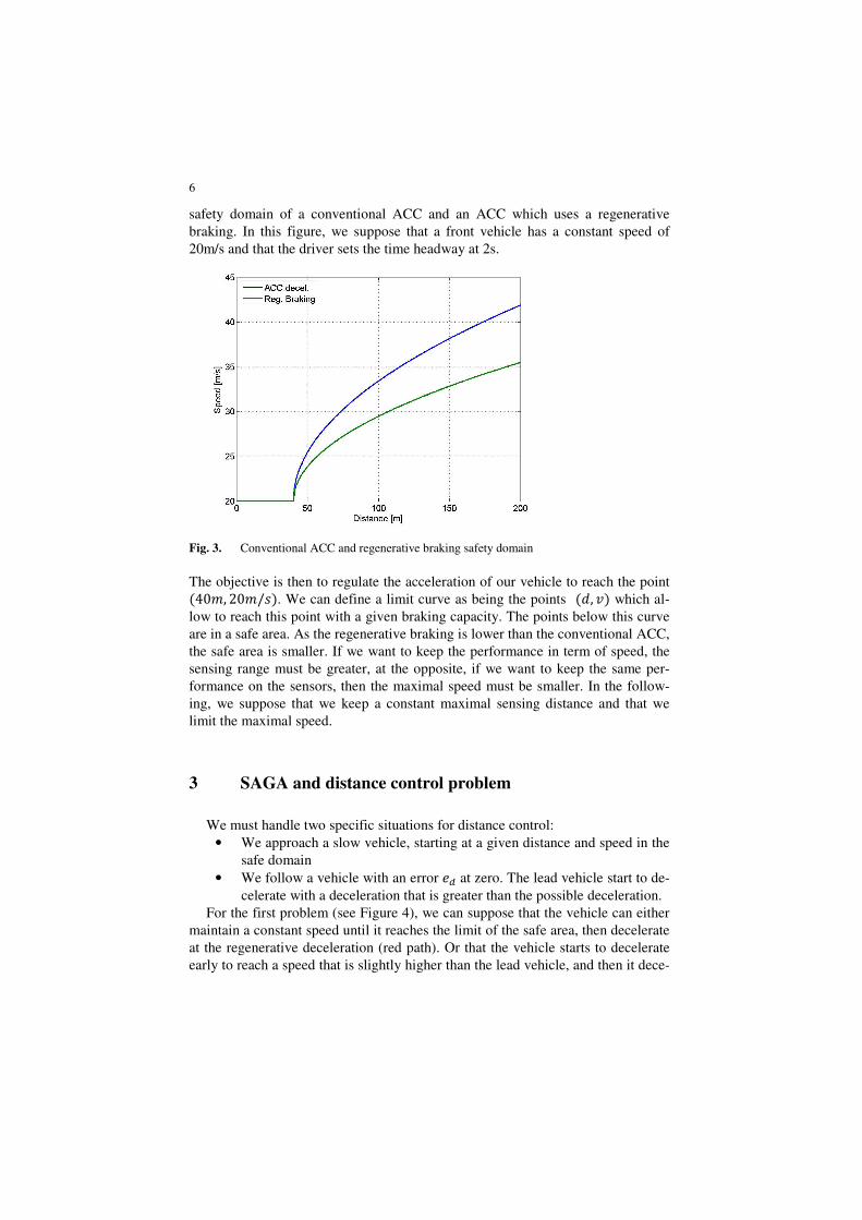
The distance control function is far more critical as it directly deals with the in-teraction between vehicles. The objective of the ACC is to regulate the error on the clearance 8 (8 % around 0. Depending on the sensors used to measure the distance, the algorithm may be more robust by integrating the error on the relative speed . The resulting acceleration is a function of this two errors, which is limited by the definition of the ACC. However, the regenerative braking is often below this threshold: with only a regenerative braking, we cannot ensure the same safety level of an ACC if we use the same strategy. Figure 3 shows the
6
safety domain of a conventional ACC and an ACC which uses a regenerative braking. In this figure, we suppose that a front vehicle has a constant speed of 20m/s and that the driver sets the time headway at 2s.
Fig. 3. Conventional ACC and regenerative braking safety domain
The objective is then to regulate the acceleration of our vehicle to reach the point 9:; <:;%. We can define a limit curve as being the points =% which al-low to reach this point with a given braking capacity. The points below this curve are in a safe area. As the regenerative braking is lower than the conventional ACC, the safe area is smaller. If we want to keep the performance in term of speed, the sensing range must be greater, at the opposite, if we want to keep the same per-formance on the sensors, then the maximal speed must be smaller. In the follow-ing, we suppose that we keep a constant maximal sensing distance and that we limit the maximal speed.
3 SAGA and distance control problem
We must handle two specific situations for distance control: • We approach a slow vehicle, starting at a given distance and speed in the
safe domain • We follow a vehicle with an error 8 at zero. The lead vehicle start to de-
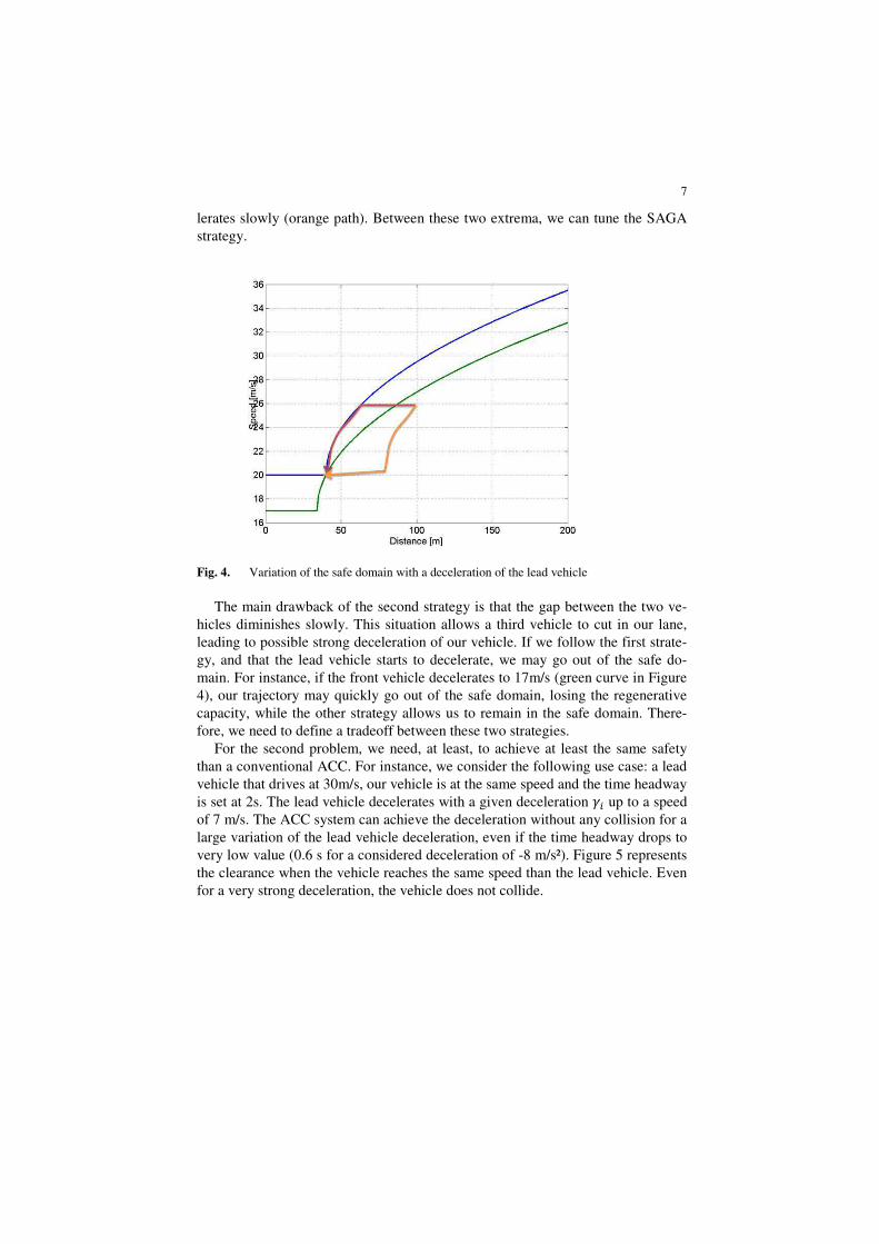
celerate with a deceleration that is greater than the possible deceleration. For the first problem (see Figure 4), we can suppose that the vehicle can either
maintain a constant speed until it reaches the limit of the safe area, then decelerate at the regenerative deceleration (red path). Or that the vehicle starts to decelerate early to reach a speed that is slightly higher than the lead vehicle, and then it dece-
7
lerates slowly (orange path). Between these two extrema, we can tune the SAGA strategy.
Fig. 4. Variation of the safe domain with a deceleration of the lead vehicle
The main drawback of the second strategy is that the gap between the two ve-hicles diminishes slowly. This situation allows a third vehicle to cut in our lane, leading to possible strong deceleration of our vehicle. If we follow the first strate-gy, and that the lead vehicle starts to decelerate, we may go out of the safe do-main. For instance, if the front vehicle decelerates to 17m/s (green curve in Figure 4), our trajectory may quickly go out of the safe domain, losing the regenerative capacity, while the other strategy allows us to remain in the safe domain. There-fore, we need to define a tradeoff between these two strategies.
For the second problem, we need, at least, to achieve at least the same safety than a conventional ACC. For instance, we consider the following use case: a lead vehicle that drives at 30m/s, our vehicle is at the same speed and the time headway is set at 2s. The lead vehicle decelerates with a given deceleration up to a speed of 7 m/s. The ACC system can achieve the deceleration without any collision for a large variation of the lead vehicle deceleration, even if the time headway drops to very low value (0.6 s for a considered deceleration of -8 m/s²). Figure 5 represents the clearance when the vehicle reaches the same speed than the lead vehicle. Even for a very strong deceleration, the vehicle does not collide.

8
Fig. 5. Final clearance as a function of the deceleration of the lead vehicle
Using the regenerative deceleration only, it is not possible to obtain the same safety level than a conventional ACC with the same use case (initial time headway of 2 s, speed of 30 m/s and final speed of the lead vehicle of 7 m/s). The possible solutions are:
• To increase the minimal time headway that is defined by the driver. However, to obtain the same safety, we need to increase the minimal time headway up to 5s. The resulting distance is hardly achievable as the sen-sor range is limited and other road user may cut in the space between ve-hicles.
• To switch to conventional braking if the time headway drops below a given threshold. For instance, we can maintain a collision free system, as for a conventional ACC, with an initial time headway of 3.7s and an acti-vation of a stronger braking at a threshold on the time headway of 1.5s
• To switch to an emergency braking if the deceleration of the lead vehicle and the distance drops below given thresholds. If the emergency braking can generate a deceleration of -6m/s² when the time to collision (differ-ence of distance divided by the difference of speed) is below 2s, we can set the minimal time headway at 3s.
As we want to use only the ACC system, then we choose the second option. However, we do not evaluate the acceptability by the user of the resulting clear-ance.
9
4 Simulation results
In the following, we develop two different use cases to present the efficiency of the system. In a first scenario, our vehicle drives at the driver desired speed and it approaches a slow vehicle. The second scenario shows the reaction on a cut in sit-uation. The new target first decelerates slowly to increase the clearance with the previous lead vehicle, then accelerates to reach the traffic flow speed.
In the following, the ACC aims to regulate the distance at an headway of 2s, the SAGA parameter is at 3.5s. For SAGA, we use the conventional ACC if the headway drops below 1.2s, and we start to control the vehicle with a 20% longer distance.
4.1 Approaching a slow vehicle
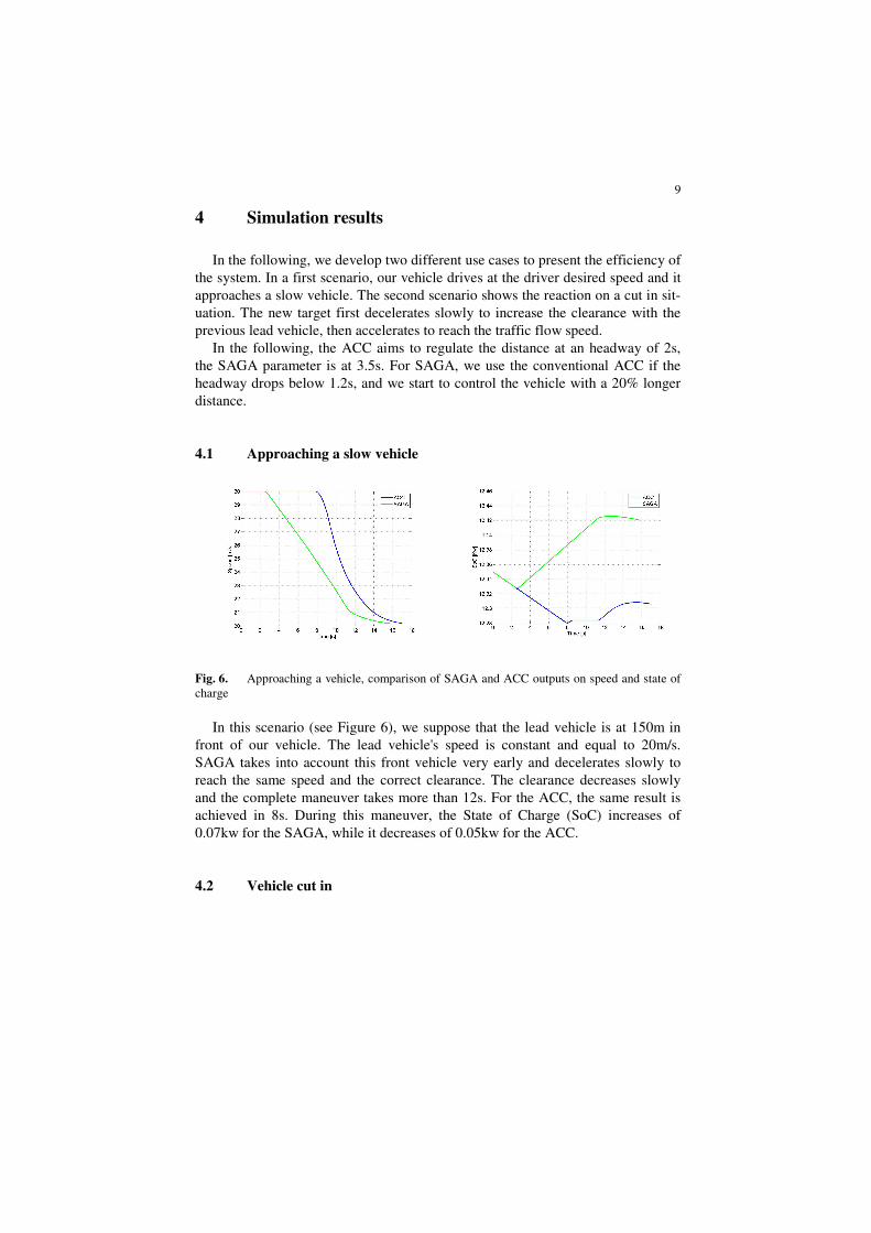
Fig. 6. Approaching a vehicle, comparison of SAGA and ACC outputs on speed and state of charge
In this scenario (see Figure 6), we suppose that the lead vehicle is at 150m in front of our vehicle. The lead vehicle's speed is constant and equal to 20m/s. SAGA takes into account this front vehicle very early and decelerates slowly to reach the same speed and the correct clearance. The clearance decreases slowly and the complete maneuver takes more than 12s. For the ACC, the same result is achieved in 8s. During this maneuver, the State of Charge (SoC) increases of 0.07kw for the SAGA, while it decreases of 0.05kw for the ACC.
4.2 Vehicle cut in
10
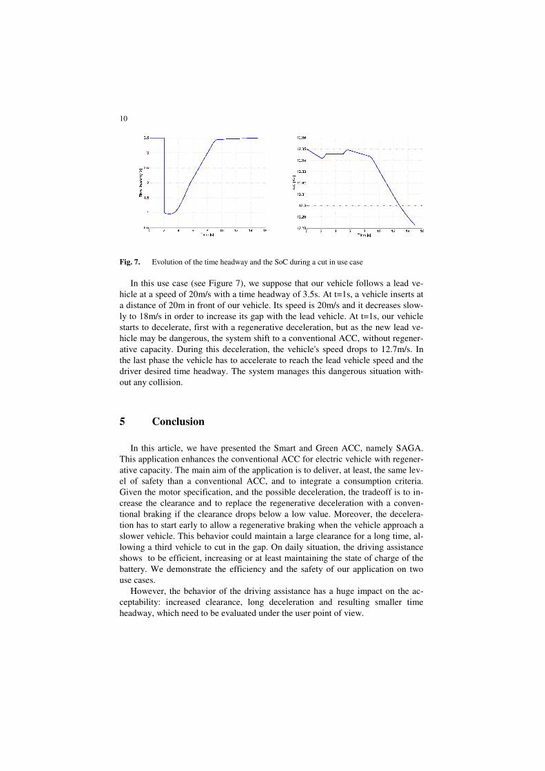
Fig. 7. Evolution of the time headway and the SoC during a cut in use case
In this use case (see Figure 7), we suppose that our vehicle follows a lead ve-hicle at a speed of 20m/s with a time headway of 3.5s. At t=1s, a vehicle inserts at a distance of 20m in front of our vehicle. Its speed is 20m/s and it decreases slow-ly to 18m/s in order to increase its gap with the lead vehicle. At t=1s, our vehicle starts to decelerate, first with a regenerative deceleration, but as the new lead ve-hicle may be dangerous, the system shift to a conventional ACC, without regener-ative capacity. During this deceleration, the vehicle's speed drops to 12.7m/s. In the last phase the vehicle has to accelerate to reach the lead vehicle speed and the driver desired time headway. The system manages this dangerous situation with-out any collision.
5 Conclusion
In this article, we have presented the Smart and Green ACC, namely SAGA. This application enhances the conventional ACC for electric vehicle with regener-ative capacity. The main aim of the application is to deliver, at least, the same lev-el of safety than a conventional ACC, and to integrate a consumption criteria. Given the motor specification, and the possible deceleration, the tradeoff is to in-crease the clearance and to replace the regenerative deceleration with a conven-tional braking if the clearance drops below a low value. Moreover, the decelera-tion has to start early to allow a regenerative braking when the vehicle approach a slower vehicle. This behavior could maintain a large clearance for a long time, al-lowing a third vehicle to cut in the gap. On daily situation, the driving assistance shows to be efficient, increasing or at least maintaining the state of charge of the battery. We demonstrate the efficiency and the safety of our application on two use cases.
However, the behavior of the driving assistance has a huge impact on the ac-ceptability: increased clearance, long deceleration and resulting smaller time headway, which need to be evaluated under the user point of view.
11
6 References
[1] Marsden G., McDonald M., Brackstone M., Marsden G., Towards an understanding of adaptive cruise control, Transportation Research Part C 9 (2001) 33-51
[2] Kesting A., Trieber M., Schonhof M., Helbing D., Extending adap-tive cruise control to adaptive driving strategies, Transportation Re-search Record: Journal of the transportation research board, N2000, 2007, pp 16-24
[3] Vahidi A., Eskandarian A., Research advances in intelligent collision avoidance and adaptive cruise control, IEEE Transactions on Intelligent Transportation Systems, 4(3), 143-153.
[4] Moon S., Moon I., Yi K., Design, tuning,and evaluation of a full-range adaptive cruise control system with collision avoidance, Control Engineering Practice (2009)442-455
[5] Naus G., Vugts R., Ploeg J., van de Molengraft R., Steinbuch M., Cooperative Adaptive Cruise Control, IEEE Automotive Engineering Symposium Eindhoven, The Netherlands, April 6, 2009
[6] Van Arem B., Van Driel C.J.G. and Visser R., The impact of cooper-ative adaptive cruise control on traffic flow characteristics, IEEE Trans-actions on Intelligent Transportation Systems, Vol. 7, No. 4, pp. 429-436, Dec. 2006
[7] Nowakowski C, Shladover S.E., Cody D. et al., Cooperative Adap-tive Cruise Control: Testing Drivers Choices of Following Distances, UCB-ITS-PRR-2010-39
[8] ISO 15622:2010, Intelligent transport system, Adaptive Cruise Con-rol system, performance requirements and test procedures
[9] Glaser S., Aguilera V., Vehicle Infrastructure Driver Speed Profile : Towards the next Generation of Curve Warning Systems, In Proc. of the 10th ITS World Congress, Madrid, Spain, nov. 2003.
[10] Aguilera V., Glaser S., Von Arnim A., An advanced Driver Speed Assistance in Curves : risk function, cooperation modes, system archi-tecture and experimental Validation. In Proc. of the IEEE Intelligent Vehicle Symposium, Las Vegas, 2005.

12
7 Full Author information
Sebastien GLASER LIVIC, 14 route de la minière Bat 824 78000 Versailles France E-mail: [email protected]
Sagar Akhegaonkar INTEDIS GmbH & Co. KG, Max-Mengeringhausen-Strae 5 97084 Wuerzburg Germany E-mail: [email protected]
Olivier Orfila LIVIC, 14 route de la minière Bat 824 78000 Versailles France E-mail: [email protected]
Lydie Nouveliere LIVIC, 14 route de la minière Bat 824 78000 Versailles France E-mail: [email protected] Frederic Holzmann INTEDIS GmbH & Co. KG, Max-Mengeringhausen-Strae 5 97084 Wuerzburg Germany E-mail: [email protected] Volker Scheuch INTEDIS GmbH & Co. KG, Max-Mengeringhausen-Strae 5 97084 Wuerzburg Germany E-mail: [email protected]

13
8 Keywords
Driving assistance, longitudinal control, energy efficiency
An improved approach for robust road marking detection and tracking
applied to multi-lane estimation.
Marc Revilloud, Dominique Gruyer IEEE Member, Evangeline Pollard
Abstract— In this paper, an original and innovative algorithmfor multi-lane detection and estimation is proposed. Based ona three-step process, (1) road primitives extraction, (2) roadmarkings detection and tracking, (3) lanes shape estimation.This algorithm combines several advantages at each processinglevel and is quite robust to the extraction method and morespecifically to the choice of the extraction threshold. Thedetection step is so efficient, by using robust poly-fitting basedon the point intensity of extracted points, that correction step isalmost not necessary anymore. This approach has been used inseveral project in real condition and its performances have beenevaluated with the sensor data generated from SiVIC platform.This validation stage has been done with a sequence of 2500simulated images. Results are very encouraging : more than95% of marking lines are detected for less than 2% of falsealarm, with 3 cm accuracy at a range of 60 m.
I. INTRODUCTION
For at least two decades, the development of transporta-
tion systems have led to the developement of embedded
applications allowing to improve the driving comfort and to
minimize the risk level of hazardous areas. More specificaly,
the researches in intelligent and Advance Driving Assistance
Systems have provided a great number of devices on many
types of automatic vehicle guidance and security systems
such as obstacle detection and tracking [1], road visibility
measurement [2], pedestrian detection, road departure warn-
ing systems.... However, one of the first embedded system
that was studied is probably the lane detection system.
This application is usually based on road marking detection
algorithms. [3]. This system is also one of the most important
source of information in order to build a local perception map
of an environment surrounding an ego-vehicle. Indeed, this
information provides relative vehicle location information to
all other perception systems (obstacles, road signs, ...) that
need to know the road and lanes attributes. For this reason the
system must be as robust as possible. Moreover, for several
year, it appears evident the automation of the driving task
is probably a solution in the reduction of the road injuries.
But for automated or partially automated driving task, the
road marking and lane localization are very important and
provide a critical information. This information needs to be
really accurate, certain, reliable in order to achieve some
manoeuvers like lane changes or generate safe path planing
(co-pilot) [4].
M. Revilloud and D. Gruyer are with the LIVIC research laboratory,IFSTTAR, 14 route de la Miniere, bat 824, 78000 Versailles, France
E. Pollard is with the INRIA Paris-Rocquencourt research laboratory, inthe project-team IMARA [email protected]
The research and the study proposed in this paper are
directly dedicated to this important topic of road markings
detection and tracking , and lanes estimation for automated
and/or partialy automated driving applications. Our objective
is to provide an assessment of the road surface attributes
(road markings attributes, type of road marking, number of
lane and characteristic of lanes). This method is based on
use of one or several embedded cameras.
Most of the algorithms are basically based on a three-step
scheme summarized as follows. First, images are processed
in order to extract road marking features. Second, extracted
primitives are analyzed in order to extract point distributions
corresponding to a road marking. And finally in a third
step, extracted and validated points are used to extract lane
shape. In some previous work [5], the first extraction part
has been studied, tested, and evaluated in order to determine
the best way to extract road marking primitives. In this
paper, a double extraction strategy is proposed to achieve
the discimination of the points for marking points and non-
marking points. To guaranty the robustness of our approach,
we proposed in addition a performance evaluation protocol
for the first road primitives extraction stage based on the
use of the SiVIC platform, which is presented in [6]. This
protocol provides an accuracy measurement of the clustering
and robustness relatively to a clustering threshold Tg .
In this paper, we present several significant improvements
of the original method proposed by S. S. Ieng and D.
Gruyer in [7]. The global scheme is the same one but some
enhancements have been done in each part. For instance, the
combination strategy of several extractors, the management
of the primitives in the detection stage, and the lane and
markings estimation in the lane estimation part has been
modified. In addition, instead of imposing a very discrim-
inative threshold into the extraction part, we propose the use
of the intensity of the extracted point into both the detection
and the estimation parts. Lane marking detection, originally
based on the study of an histogram containing projected
points, is now made by using the same type of histogram
but where the projected point are weighted in function of
their uncertainty. Moreover, the poly-fitting mechanism has
been replaced by a a weighted poly-fitting, for the same
reason. Higher is the extracted intensity points, more strongly
weighted are these points in the estimation process. To
robustify our approach and avoid false alarms, distribution
points which are not satisfying very discriminative criteria
for peak clustering are submitted to a robust weighted poly-
fitting. In this way, point distributions containing outliers (as
it could happen in the case of sidewalks or guardrail which
2013 IEEE Intelligent Vehicles Symposium (IV)June 23-26, 2013, Gold Coast, Australia
978-1-4673-2754-1/13/$31.00 ©2013 IEEE 783

produce false alarms), are still validated as road markings.
Finally, comparatively to the initial version of this algorithm,
the proposed improvements lead to better results. These
changes in the different part of this method allow to affirm
that the use of the filtering step is not important anymore.
The Fig. 1 gives an global overview of the proposed
road marking detection and tracking and lane estimation
architecture. The paper is organized as follows. In Sec. II, the
Fig. 1. The entire process for road marking detection
SiVIC platform used for the evaluation of marking detection
is presented. In Sec. III, the three main parts of this approach
are detailed. Sec. IV described the evaluation protocol used
for road marking detection algorithm. Sec. V presents a set
of results with differents road conditions and levels of quality
for the road markings.
II. THE SIVIC PLATFORM
SiVIC is a virtual sensor simulation platform for ADAS
prototyping. It simulates different embedded sensors (cam-
era, telemeters, GPS, radar, communication devices, INS,
odometer ...) and the dynamic vehicle behaviour of vehicle
as described in [6]. In order to prototype and to test ADAS,
a realistic 3D reproduction of the real Satory’s test track
was produced by LIVIC. Fig. 2 shows the similarity of
this simulation in comparison with the same perspective on
the real track. In this figure, the first line provides virtual
renderings and the second line gives the real pictures from
the same point of view. This simulation takes into account
a great number of detail such as as the road shape, guard
rails, buildings, road sign elements, trees, etc. The images
generated by the SiVIC platform can be considered relatively
close to the images which could be provided by a real camera
Fig. 2. The quality of this virtual platform is mainly due to:
• The high accuracy of both the shapes of the Satory’s
track (build from a centimetric GPS-RTK) and the ad-
ditional element of the environment (buiding, guardrail,
sidewalk, trees, road signes, differents fences, ...)
• Natural images of bitumen used as road textures
Fig. 2. Comparison of SIVIC and natural images
• The realistic model of the vehicle dynamics
• An accurate modeling of the optical sensor as describe
in [8]
• The capabilities of SiVIC to provide both camera im-
ages and the associated ground truth.
III. ROAD MARKING DETECTION AND ESTIMATION
On the same principle as [7], a three step process for
lane marking detection and estimation is proposed. The main
purpose is to obtain the number of lane markers Nk, their
position and their shape. For each validated lane marker m,
the goal is also to provide an estimation of the road shape as
a second degree polynomial in the vehicle coordinate system
x = am0 + am1 · y + am2 · y2 (1)
As illustrated in Fig. 1, the first step consists in extracting
road marking primitives. The second step is dedicated to the
association stage. In fact from a set of extracted primitives,
the objective is to detect the number of road markings and to
associate them with the last ones (the road marking tracks).
In a third step, given a set of labeled primitives, the goal is
to provide, for each frame k, an estimation of the real state
Am,k of any road marking m:
Am,k =[
amk,0, amk,1, a
mk,2
]T(2)
corresponding to eq. (1), where (·)T denotes the transpose
transformation. With this information, an associated uncer-
tainty matrix Pm,k is also estimated.
A. Lane marker feature extraction
The first step consists also in establishing which input
image points belong to a lane marker. Most of the time, lane
marker forms bright region (white or yellow paint) on a dark
background (asphalt), having a limited width. Extraction pur-
pose is also to detect regions with a gradient intensity higher
than a certain threshold Tg and bounded by the interval
[Sm, SM ]. It has been shown in [9], that local thresholding
methods provide the best results. In some previous work [10],
a protocol was proposed for the evaluation of road marking
784

extraction algorithms, based on synthesized images coming
from simulator Sivic. After a study about performances of
four extraction algorithms based on local thresholding, we
proposed a new lane feature extraction algorithm based on
a double extraction scheme. However, experimental results
show that the assumption that better are the extraction step
(using the procole used in [5]), more accurate is the road
state estimation is uncorrect. Results presented in Sec. V
prove that with the improvement of detection part, if double
extraction scheme does not degrade performances, it does
not improve it and necessarily increases time processing.
Extraction step is also limited to SLT (Symmetric Local
Threshold) in order to provide a set of extracted points E
and their corresponding intensity.
Finally, to enable the processing of extracted point, each
extracted point of each cameras are projected in the vehi-
cle coordinate system. This projection stage uses intrinsic
and extrinsic parameters of the camera which are known.
The position is fixed, perpendicularly to the car frame.
The origin of the camera coordinate system Rcam =(Ocam, ~Xcam, ~Ycam, ~Zcam) is also established at coordinates
(0, 0, h) in the vehicle coordinate system, denoted Rv =(Ov, ~Xv, ~Yv, ~Zv), as illustrated in Fig. 3, with h the height
of the camera knowing the car reference. This coordinate
system is centered on the car referential, perpendicularly to
the road surface, assumed to be plane.
Fig. 3. Observation and coordinate system
B. Lane marker detection
1) Point projection: Knowing the set of extracted points
E (cf. Fig. 4-(a)), the goal is now to detect marking lines
and label extracted points according to detected lines. Their
associated intensity is used in addition in order to take
into account their uncertainty. Even if Hough transformation,
traditionally used to detect straight lines can be extended to
curves [11], the proposed approach is based on an analysis
of the spatial distribution of extracted points on the Xv
axis. Xv space is first cut into constant space intervals
between Xminv and Xmax
v . Contrary to [3], where points
are projected along the Yv axis, our 2D-detected points are
projected along the road shape on the Xv axis. They are
projected between 1 and 255 times depending on the value
of their intensity. Shape of the road is established by using
best available estimation states. More details are given to
define what is a good estimation in Sec. III-F. According
to its projection state xpi , each point i (∀i ∈ 1, . . . , n)
given by primitive extraction step illustrated in Fig. 4-(a) and
projected to vehicle coordinate system, can be associated to
a x-interval corresponding to a dynamic projection template,
illustrated in Fig. 4-(b). A point density histogram is then
constructed. To distinguish marking lines to false alarms
and to precisely establish peak coordinates, the histogram
is convoluted with a Normal distribution N (·, (σci )
2) with a
variance (σci )
2 corresponding to the width of two histogram
intervals, as shown in Fig. 4-(c). Histogram peaks correspond
to marking lines. The next step consists in precisely and
reliably detect histogram peaks.
Fig. 4. Marking line detection
It has been shown in [12], that a non-Gaussian model
is more adapted to describe perturbations on the observa-
tion of lane markers. Ieng et al. also propose to model
noise measurements as a Smooth Exponential Family (SEF)
distribution defined according parameters α and ζ. The
approach consists in detecting error minima by calculating
zero crossing of the following third derivative (illustrated in
Fig. 4-(d)) of the error function φα:
∂3φα
∂t3=
4t
ζ4
(
1 +t2
ζ2
)(α−3)
(α− 1)
(
3 +t2
ζ2(2α− 1)
)
(3)
Zero crossing corresponds to the projected position Xpm
of potential marking lines.
2) Peak validation: Peaks are first filtered according to
the number of points: the number of points forming the peak
must be higher than the minimum number of points Nmin.
Sets of labeled points (labeled according to the peak label)
are written under a matrix form as:
Xm,k =
1 x1 x21
......
...
1 xNmx2Nm
, Ym,k =
y1...
yNm
(4)
The polynomial fit of Am,k, denoted Am,k is obtained by
using a weighted least squares estimation as follows:
Am,k = (XTm,kWm,kXm,k)
−1XTm,kWm,kYm,k (5)
785
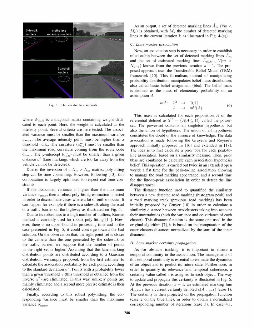
Fig. 5. Outliers due to a sidewalk
where Wm,k is a diagonal matrix containing weight dedi-
cated to each point. Here, the weight is calculated as the
intensity point. Several criteria are here tested. The associ-
ated variance must be smaller than the maximum variance
σmax. The average intensity point must be higher than a
threshold γmin. The curvature (amk,2) must be smaller than
the maximum road curvature coming from the route code
θmax. The y-intercept (amk,0) must be smaller than a given
distance d0 (lane markings which are too far away from the
vehicle cannot be detected).
Due to the inversion of a Nm × Nm matrix, poly-fitting
step can be time consuming. However, following [13], this
computation is largely optimized to respect real-time con-
straints.
If the associated variance is higher than the maximum
variance σmax, then a robust poly-fitting estimation is tested
in order to discriminate cases where a lot of outliers occur. It
can happen for example if there is a sidewalk along the road
or a traffic barrier on the highway as illustrated on Fig. 5.
Due to its robustness to a high number of outliers, Ransac
method is currently used for robust poly-fitting [14]. How-
ever, there is no upper bound in processing time and in the
case presented in Fig. 5, it could converge toward the bad
solution. On the observation that, the right point set is closer
to the camera than the one generated by the sidewalk or
the traffic barrier, we suppose that the number of points
in the right set is higher. Assuming that the lane marking
distribution points are distributed according to a Gaussian
distribution, we simply proposed, from the first estimate, to
calculate the association probability for each point, according
to the standard deviation σr. Points with a probability lower
than a given threshold γ (this threshold is obtained from the
inverse χ2) are eliminated. In this way, unlikely points are
mainly eliminated and a second more precise estimate is then
calculated.
Finally, according to this robust poly-fitting, the cor-
responding variance must be smaller than the maximum
variance σrmax.
As an output, a set of detected marking lines Am (∀m <
Mk) is obtained, with Mk the number of detected marking
lines at the current iteration k as illustrated in Fig. 4-(e)).
C. Lane marker association
Now, an association step is necessary in order to establish
relationship between the set of detected marking lines Am
and the set of estimated marking lines Am,k−1 ∀(m <
Nk−1) known from the previous iteration k − 1. The pro-
posed approach uses the Transferable Belief Model (TBM)
framework [15]. This formalism, instead of manipulating
probability distribution, manipulates belief mass distribution,
also called basic belief assignment (bba). The belief mass
is defined as the mass of elementary probability on an
assumption A:
mΩ : 2Ω → [0, 1]A → mΩ(A)
(6)
This mass is calculated for each proposition A of the
referential defined as 2Ω = A|A ⊆ Ω called the power-
set. The power-set contains all singleton hypothesis, but
also the union of hypotheses. The union of all hypotheses
constitutes the doubt or the absence of knowledge. The data
association is made following the Gruyer’s and Royere’s
approach initially proposed in [16] and extended in [17].
The idea is to first calculate a prior bba for each peak-to-
line association, based on a similarity measure. Then, prior
bbas are combined to calculate each association hypothesis
belief. This operation is carried out twice in an extended open
world: a fist time for the peak-to-line association allowing
to manage the road marking appearance, and a second time
for the line-to-peak association in order to detect the line
disappearance.
The distance function used to quantified the similarity
between a new detected road marking (histogram peak) and
a road marking track (previous road marking) has been
initially proposed by Gruyer [18] in order to calculate a
similarity distance between two clusters taking into account
their uncertainties (both the variance and co-variance of each
cluster). This distance function is the same one used in the
original algorithm [7], it is based on the computation of the
outer clusters distances normalized by the sum of the inner
distances.
D. Lane marker certainty propagation
As for obstacle tracking, it is important to ensure a
temporal continuity in the association. The management of
this temporal continuity is essential to estimate the dynamics
of an object and to predict its future state. Furthermore, in
order to quantify its relevance and temporal coherence, a
certainty value called c is assigned to each object. The way
to update and propagate this certainty is illustrated in Fig. 6.
At the previous iteration k − 1, an estimated marking line
Am,k−1 has a current certainty denoted c(Am,k−1) (case 1).
The certainty is then projected on the propagation function
(case 2 on the blue line), in order to obtain a normalized
corresponding number of iterations (case 3). In case 4.1,
786

Fig. 6. Certainty with n′ the normalized number of iterations
Fig. 7. Certainty propagation
the estimated object Am,k−1 is associated to a detected
object Am′ . In this case, the corresponding relative number
of iterations increases relatively to both the belief into this
association mΩ⋆
Mk
1...Mk
Am,k−1
(
Am′
)
and the quality of
the road marking detection. This corresponding normalized
number is yet reprojected following the same propagation
function to obtain the new increased certainty c(Am,k) at
iteration k (case 5.1). In the case where the estimated line
marking is not associated, then the corresponding normalized
number of iterations decreases by 1 (case 4.1) and the cor-
responding certainty c(Am,k) also decreases. Each detected
object is initialized with a certainty c0. In the current method,
this value is fixed to 0.5 but it will be clever to initialize this
value in function of the quality of the current road marking
detection.
In the Fig. 6, the certainty propagation is made with a
linear fonction (with a slope of 1). However, in a more
generic approach,this function is chosen depending on a co-
efficient α which is fixed relatively to the data reliability and
confidence. The ability to choose a specific function, in order
to propagate a certainty, is done to model both the optimistic
and pessimistic behaviors of the certainty propagation as
shown in Fig. 7. In the optimist case, the certainty increases
quicker than in the pessimist case. The propagation function
must be chosen symmetrical, continuously increasing and
derivable. In this application, the used propagation function
is a Bezier curve as proposed in [16].
When the certainty c(Am,k) decreases until 0, the object
is deleted.
E. Lane marker estimation
Assuming that each road marking (lane marker) m is now
detected with a certainty c(Am,k) and a set of labeled points
xi, yi∀i∈1,...,Nm converted into the vehicle coordinate
system, the goal is to provide an estimation Am,k of the
road marking shape as a second degree polynomial function
as described in eq. 2.
Lane markers are not strictly constant over time and
across successive images. They can be simply estimated
using a linear Kalman filter, whom assumptions are now
described. However, they change relatively slowly assuming
a constant vehicle speed and under flat road assumption
(required assumption for the point conversion into the vehicle
coordinate) following the state equation:
Am,k+1 = Fk ·Am,k + νm,k (7)
where Fk designates the evolution matrix, Ak,m the real road
marking state at iteration k and νm,k the model noise rep-
resenting the uncertainty in the road marking evolution over
time. If some authors like [19] uses elaborated and complex
evolution matrix, we assume that the change between two
successive image is negligible (matrix Fk is equal to the
identity matrix) and can be modeled thanks to the model
noise, which must be adequately chosen. The model noise
νm,k can be estimated by studying the maxium evolution of
parameters of a road marking between iteration k and k+1.
Measurement-to-state equation can be simply written as:
Xk,m ·Ak,m = Yk,m + wk,m (8)
where wk,m represents the measurement noise estimated at
each iteration as the error of one pixel shift in the vehicle
coordinate system.
Assuming that extracted features cannot be modeled as
Gaussian distribution, Ieng et al. estimates lane marker
states by using a Robust Kalman Filter [1]. We propose as
an alternative to use a gating computation [2] and to re-
estimate road marking shape Am,k. A gate is also designed
around the predicted position at iteration k of road marking
Ak|k−1,m, based on the maximum acceptable measurement
error according to the prediction error magnitude. Only
points that are within the track gate are considered for update
the lane marker at iteration k. As shown in Fig. 8, false points
are filtered and selected points can be modeled as a Gaussian
distribution.
At this stage, Am,k are so close to the reality that a
corrective step is unnecessary and Am,k = Am,k .
787

Fig. 8. Gating process illustration
Fig. 9. Road shape interpolation in case of high curvature. (a) originalimages and its extracted points. (b) Interpolated road shape for each interval(red lines: previous road shape estimates, dotted lines: interpolated roadshape). Points are colored accordingly to their interval.
F. Road shape update
As explained in Sec. III-B, extracted points are projected
according to the global road shape. One solution consists
in selecting the best road marking estimation (best to the
point of view of varying criteria such as the number of
extracted points, and the smallest error estimation) in order
to project the points (road marking primitives) for the next
iteration. However, in case of strong curvatures, we can note
that the inside road markings have a stronger curvature than
the outside ones as illustrated in Fig. 9-(a). The proposed
solution consists in selecting several lane markers as road
shape reference. Road markings are selected if they satisfy
strict criteria (more strict than detection criteria) on:
• the number of points forming the peak must be higher
than the minimum number of points Npmin (N
pmin >
Nmin),
• the variance of the peak must be smaller than the
maximum variance σpmax (σp
max < σmax).
If several road marking estimates are selected as road
shape reference, they are first tested to detect cross road
Fig. 10. Evaluation protocol
markings (cross lane markers). In fact, they are not supposed
to cross each other. If road marking crossing is detected,
only the lane marker with the minimum variance is selected.
They are then used to interpolate a second degree polynomial
function for each interval as illustrated in Fig.9-(b).
IV. EVALUATION PROTOCOL
To evaluate the quality of this algorithm and the impact
of each parameter, an evaluation tool and a protocol have
been developed. The evaluation protocol uses the estimates
from the lane detection algorithm and ground truth images
provided by SiVIC as illustrated in Fig.10. This protocol is
based on four criteria:
• Detection rate: Rate of good detection estimated ac-
cording to the ground truth for one lane. This rate
corresponds to the line ratio where distance between the
estimate and the ground truth is below a given threshold
dmin. For the l line of our image, this distance em,k,l
between the estimate Am,k,l and the the average points
of the line Tm,k,l is calculated as an Euclidian distance:
em,k,l = d(Am,k,l, Tm,k,l) (9)
where d(., .) the euclidian distance. This threshold dmin
was chosen after empirical testing of different ADAS
system.
• Precision: Accuracy in the case of correct detection for
one lane. This accuracy is calculated as the mean of
each d(l) for each line of the ground truth image.
• False alarm rate: Ratio between the number of false
detections and the real number of lanes.
• Global detection rate: Ratio between the number of
correct detections and the real number of lanes.
V. RESULTS
In this section, some results are presented according to
the dedicated performance protocol developped with the
SiVIC platform. This evaluation has been done on a Sivic
sequence of images combining several situation: straight
line, strong curvature, guardrails, sidewalks, fences, trees,
different conditions of shadows. . . . Detection rate (DR) and
false alarm rate (FAR) quantify the quality of the detection.
Detection rates per lane marking and their associated error
measure the quality of the estimation.
Numerous parameters are used in this multi-lane detection
method, which is determined before this evaluation step
788
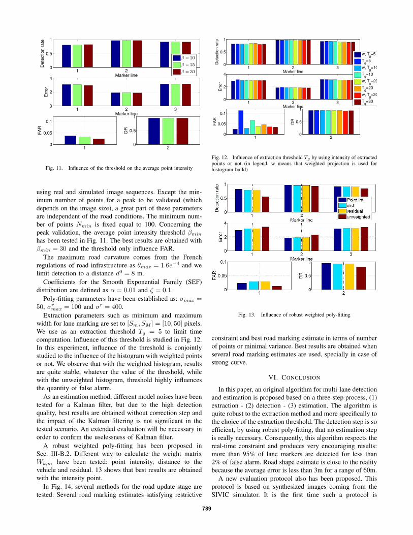
1 2 30
0.5
1
Marker line
Dete
ction r
ate
1 2 30
2
4
Marker line
Err
or
10
0.05
0.1
FA
R
20
0.5
1
DR
β = 20
β = 25
β = 30
Fig. 11. Influence of the threshold on the average point intensity
using real and simulated image sequences. Except the min-
imum number of points for a peak to be validated (which
depends on the image size), a great part of these parameters
are independent of the road conditions. The minimum num-
ber of points Nmin is fixed equal to 100. Concerning the
peak validation, the average point intensity threshold βmin
has been tested in Fig. 11. The best results are obtained with
βmin = 30 and the threshold only influence FAR.
The maximum road curvature comes from the French
regulations of road infrastructure as θmax = 1.6e−4 and we
limit detection to a distance d0 = 8 m.
Coefficients for the Smooth Exponential Family (SEF)
distribution are defined as α = 0.01 and ζ = 0.1.
Poly-fitting parameters have been established as: σmax =50, σr
max = 100 and σr = 400.
Extraction parameters such as minimum and maximum
width for lane marking are set to [Sm, SM ] = [10, 50] pixels.
We use as an extraction threshold Tg = 5 to limit time
computation. Influence of this threshold is studied in Fig. 12.
In this experiment, influence of the threshold is conjointly
studied to the influence of the histogram with weighted points
or not. We observe that with the weighted histogram, results
are quite stable, whatever the value of the threshold, while
with the unweighted histogram, threshold highly influences
the quantity of false alarm.
As an estimation method, different model noises have been
tested for a Kalman filter, but due to the high detection
quality, best results are obtained without correction step and
the impact of the Kalman filtering is not significant in the
tested scenario. An extended evaluation will be necessary in
order to confirm the uselessness of Kalman filter.
A robust weighted poly-fitting has been proposed in
Sec. III-B.2. Different way to calculate the weight matrix
Wk,m have been tested: point intensity, distance to the
vehicle and residual. 13 shows that best results are obtained
with the intensity point.
In Fig. 14, several methods for the road update stage are
tested: Several road marking estimates satisfying restrictive
1 2 30
0.5
1
Marker line
Dete
ction r
ate
1 2 30
2
4
Marker line
Err
or
10
0.05
0.1
FA
R
20
0.5
1
DR
w, Tg=5
Tg=5
w, Tg=10
Tg=10
w, Tg=20
Tg=20
w, Tg=30
Tg=30
Fig. 12. Influence of extraction threshold Tg by using intensity of extractedpoints or not (in legend, w means that weighted projection is used forhistogram build)
Fig. 13. Influence of robust weighted poly-fitting
constraint and best road marking estimate in terms of number
of points or minimal variance. Best results are obtained when
several road marking estimates are used, specially in case of
strong curve.
VI. CONCLUSION
In this paper, an original algorithm for multi-lane detection
and estimation is proposed based on a three-step process, (1)
extraction - (2) detection - (3) estimation. The algorithm is
quite robust to the extraction method and more specifically to
the choice of the extraction threshold. The detection step is so
efficient, by using robust poly-fitting, that no estimation step
is really necessary. Consequently, this algorithm respects the
real-time constraint and produces very encouraging results:
more than 95% of lane markers are detected for less than
2% of false alarm. Road shape estimate is close to the reality
because the average error is less than 3m for a range of 60m.
A new evaluation protocol also has been proposed. This
protocol is based on synthesized images coming from the
SIVIC simulator. It is the first time such a protocol is
789

Fig. 14. Result with different road shape update
implemented with virtual data in order to validate a road
marking detection method. The images provided by this
platform are quite enough realistic to effectively validate an
image processing application [8]. The evaluation protocol is
based on three criteria: the detection rate of road markings
(lane markers), the precision of their estimation and a false
alarm rate. Numerous tests on a set of parameters prove the
robustness of this approach. Finally, the proposed system has
been tested with success on several hours of data collected
on the real Satory’s test tracks under varying lighting and
curvature conditions. The real images recorded during these
trials correspond to the same one generated with the SiVIC
platform. The main goal was to obtain similar results and the
same behavior in both the real and the simulated scenarios
for autonomous driving applications. Unfortunatly, some
difficulties can appear in the road marking detection when
the vehicle is accelerating (due to the pitch) or when the flat
road assumption is not respected, but this should be solved by
integrating information on the pitch into the data conversion
stage (image space toward 1D space).
To improve the performances of this innovative approach,
numerous perspectives are possible. First, other evaluation
tests must be done to quantify the influence of moving
objects on the road. To filter primitives corresponding to
these objects, it is proposed to combine our approach with
obstacle detection algorithm (ie. from stereovision, laser, or
radar processing). Furthermore, to compensate vehicle pitch,
a new estimator will be added to apply a real time correction
in the projection module. Finally, this approach was origi-
nally made to identify the road lanes by using of a multi-
camera fusion architecture. It is therefore appropriate to
continue this multi-cameras study to quantitatively determine
the gain provided by the use of other cameras. In addition
it will be interesting to study the intrinsic and extrinsic best
configuration for this network of embedded optical sensor.
ACKNOWLEDGEMENT
This work is part of e-future, a 3-year European FP7
research project (project number: 258133) for electric car au-
tomation and of CooPerCom, a 3-year international research
project (Canada-France). The authors would like to thank the
European committee, the National Science and Engineering
Research Council (NSERC) of Canada and the National
Agency for Research (ANR) of France for supporting these
projects.
REFERENCES
[1] J.-P. Tarel, S.-S. Ieng, and P. Charbonnier, “Using Robust EstimationAlgorithms for Tracking Explicit Curves,” in ECCV 2002, ser. LectureNotes in Computer Science, A. Heyden, G. Sparr, M. Nielsen,and P. Johansen, Eds. Springer Berlin / Heidelberg, 2002, vol.2350, pp. 492–507, 10.1007 3-540-47969-4 33. [Online]. Available:http://dx.doi.org/10.1007/3-540-47969-4 33
[2] R. Sittler, “An optimal data association problem in surveillancetheory,” IEEE transactions on military electronics, vol. 8, no. 2, pp.125–139, 1964.
[3] M. Bertozzi and A. Broggi, “Gold: a parallel real-time stereo visionsystem for generic obstacle and lane detection,” IEEE Transactions on
Image Processing, vol. 7, no. 1, pp. 62 –81, Jan. 1998.[4] B. Vanholme, D. Gruyer, S. Glaser, and S. Mammar, “A legal safety
concept for highly automated driving on highways,” in Intelligent
Vehicles Symposium (IV), 2011 IEEE. IEEE, 2011, pp. 563–570.[5] E. Pollard, D. Gruyer, J. Tarel, S. Ieng, and A. Cord, “Lane marking
extraction with combination strategy and comparative evaluation onsynthetic and camera images,” in Intelligent Transportation Systems
(ITSC), 2011 14th International IEEE Conference on. IEEE, 2011,pp. 1741–1746.
[6] D. Gruyer, S. Glaser, and B. Monnier, “Sivic, a virtual platform foradas and padas prototyping, test and evaluation,” in FISITA 2010 World
Automotive Congress, Budapest, Hungary, 2010.[7] S. Ieng, J. Vrignon, D. Gruyer, and D. Aubert, “A new multi-lanes
detection using multi-camera for robust vehicle location,” in Proc. on
thee IEEE Intelligent Vehicles Symposium. IEEE, 2005, pp. 700–705.[8] D. Gruyer, M. Grapinet, and P. De Souza, “Modeling and validation of
a new generic virtual optical sensor for adas prototyping,” in Intelligent
Vehicles Symposium (IV), 2012 IEEE. IEEE, 2012, pp. 969–974.[9] T. Veit, J. Tarel, P. Nicolle, and P. Charbonnier, “Evaluation of road
marking feature extraction,” in IEEE 11th International Conference
on Intelligent Transportation Systems. IEEE, 2008, pp. 174–181.[10] E. Pollard, D. Gruyer, J.-P. Tarel, S.-S. Ieng, and A. Cord, “Lane
marking extraction with combination strategy and comparative evalu-ation on synthetic and camera images,” in Intelligence Transportation
System Conference, 2011.[11] B. Yu and A. Jain, “Lane boundary detection using a multiresolution
hough transform,” in Proceedings of the International Conference on
Image Processing, vol. 2. IEEE, 1997, pp. 748–751.[12] S. Ieng, J. Tarel, and P. Charbonnier, “Modeling non-gaussian noise
for robust image analysis,” in Proceedings of International Conference
on Computer Vision Theory and Applications. Citeseer, 2007, pp.175–182.
[13] B. Flannery, W. Press, S. Teukolsky, and W. Vetterling, “Numericalrecipes in c,” Press Syndicate of the University of Cambridge, New
York, 1992.[14] Z. Kim, “Robust lane detection and tracking in challenging scenarios,”
IEEE Transactions on Intelligent Transportation Systems, vol. 9, no. 1,pp. 16 –26, march 2008.
[15] P. Smets, “The combination of evidence in the transferable beliefmodel,” IEEE Transactions on Pattern Analysis and Machine Intel-
ligence, vol. 12, no. 5, pp. 447–458, 1990.[16] D. Gruyer, “Etude du traitement de donnees imparfaites pour le suivi
multi-objets: Application aux situations routieres,” Ph.D. dissertation,1999.
[17] C. Royere, D. Gruyer, and V. Cherfaoui, “Data association with believetheory,” in International Conference on Information Fusion, vol. 1,2000, pp. 2–3.
[18] D. Gruyer, C. Royere, and V. Cherfaoui, “Heterogeneous multi-criteriacombination with partial or full information,” Fusion03 29, p. 1,2003.
[19] B. Southall and C. Taylor, “Stochastic road shape estimation,” inComputer Vision, 2001. ICCV 2001. Proceedings. Eighth IEEE In-
ternational Conference on, vol. 1, 2001, pp. 205 –212 vol.1.
790

Weighted V-disparity Approach for Obstacles Localization in Highway
Environments
Nizar Fakhfakh1, Dominique Gruyer1 and Didier Aubert2
Abstract— The employment of embedded passive sensorsin order to perceive environment for reducing the accidentrisk level is a tendency of intelligent vehicles research. Fromsuch sensors, one can extract useful informations which canassist the driver to identify hazardous situations. While safetyimprovement is a substantial requirement for driving assistance,localizing and tracking obstacles in complex road environmentbecame an important task. One promising approach is touse the V-disparity based on the stereovision technique. It isa cumulative space estimated from the disparity image. Wepropose a sound framework and a complete system basedon a real-time stereovision for detection, 3D localization andtracking of dynamic obstacles in highway environment. Themain contribution we propose is the improvement of the V-disparity approach by extending the basic approach by mergingit with a confidence term. This consists on weighting eachpixel in the V-disparity space according to a confidence valuewhich measures the probability of associating a pair of pixels.Furthermore, we propose a tracking system which is based onthe belief theory. The tracking task is done on the image spacewhich takes into account uncertainties, handles conflicts, andautomatically dealt with targets appearance and disappearceas well as their spatial and temporal propogation. Extensiveexperiments on simulated and real dataset demonstrate theeffectiveness and the robustness of the weighted V-disparityapproach.
I. INTRODUCTION
Establishing vehicle-infrastructure-driver interactions de-
pends on the effectiveness of the perception task in a specific
road scenario. The outstanding development of hardware
have significantly improved the capabilities of embedded
algorithms for accidents avoidance and drivers’ safety im-
provement. One of the early researche works introducing
stereovision for road obstacles detection and road-line mark-
ings extraction is the one that is proposed in [1]. Unfortu-
nately, this previous work has proposed a sparse disparity
map and the detection of obstacles is not performed in real
time. The use of binocular stereopsis principle for collision
avoidance or mitigation has been first successfully demon-
strated by JPL’s planetary robotic vehicle [2] which presents
a trade-off between the computational time and the density
of the disparity map. The authors in [3] uses vision-based
detectors for estimating of the road profile. This is done by
detecting road-line markings and all of obstacles not lying on
the road plane are discarded. In [4] the authors have proposed
1N. Fakhfakh and D. Gruyer are with French Institute of Sci-ence and Technology for Transport, Development and Networks, LIVICunit. 14, route de la Miniere, Bat 824. -78000 Versailles - Satory.nizar.fakhfakh, [email protected]
2D. Aubert is with French Institute of Science and Technology for Trans-port, Development and Networks, LEPSIS unit. 58, boulevard Lefebvre,75732 Paris Cedex 15. [email protected]
an approach for the construction of occupancy grids using
stereo camera pair for obstacles detection implemented on
a GPU. Their method considers the geometrical visibility of
the different regions of the image and can deal with partially-
occluded objects. In [5] the regions so that a fixed-size
volume contains a sufficient number of points are considered
as potential obstacles.
In this paper, we propose a real-time video-based ob-
stacles localization and tracking system at daytime which
makes extensive use of stereovision principle. The proposed
system allows detecting, localizing and tracking obstacles
in highway environments in daytime. After a digitalization
and a pre-processing stage, a stereo algorithm based on a
local approach is then performed for dense disparity map
generation from which the U- and V-disparity maps are
built. The proposed work fits into earlier work initiated in
[6] which exploits the cumulative spaces termed U- and
V-disparity. The main contribution of this paper is in the
improvement of the V-disparity approach by extending the
basic approach by merging it with a confidence approach.
This consists on weighting each pixel in the V-disparity
space according to a confidence value which measures the
probability of associating a pair of pixels. The two maps, U
and V-disparity, are useful for estimating the 2D bounding
box for each potential obstacle. A set of targets is therefore
obtained with a state vector for each target. Each state vector
contains the lateral and longitudinal position, the bounding
box parameters and the uncertainty information. We have
introduced a tracking filter with an association step based on
belief theory and a filtering step using a linear Kalman filter.
The association step allows to provide a link between a target
and a track. The filter provide an update of the track state
vector given the target data. This allows decreasing false
positive rate and avoiding missed detections. The tracking
task is done on the image space and allows taking into
account uncertainties, handles conflicts, and automatically
dealt with the appearance and the disappearing of targets
as well as their spatial and temporal propogation. Then, the
objects which are not lying in the road plane and hence
non-potential obstacles are removed. The remaining potential
obstacles are kept and are subject for further treatment.
Section II provides a brief overview of the proposed
system. Section III gives the first contribution of this work
with the presentation of an improved dense disparity map
building with confidence approach applied to each pixel.
This confidence approach is used to improve the V-disparity
approach. Section IV explains the second contribution dedi-
cated to the tracking stage using probabilistic approach and
2013 IEEE Intelligent Vehicles Symposium (IV)June 23-26, 2013, Gold Coast, Australia
978-1-4673-2754-1/13/$31.00 ©2013 IEEE 1271
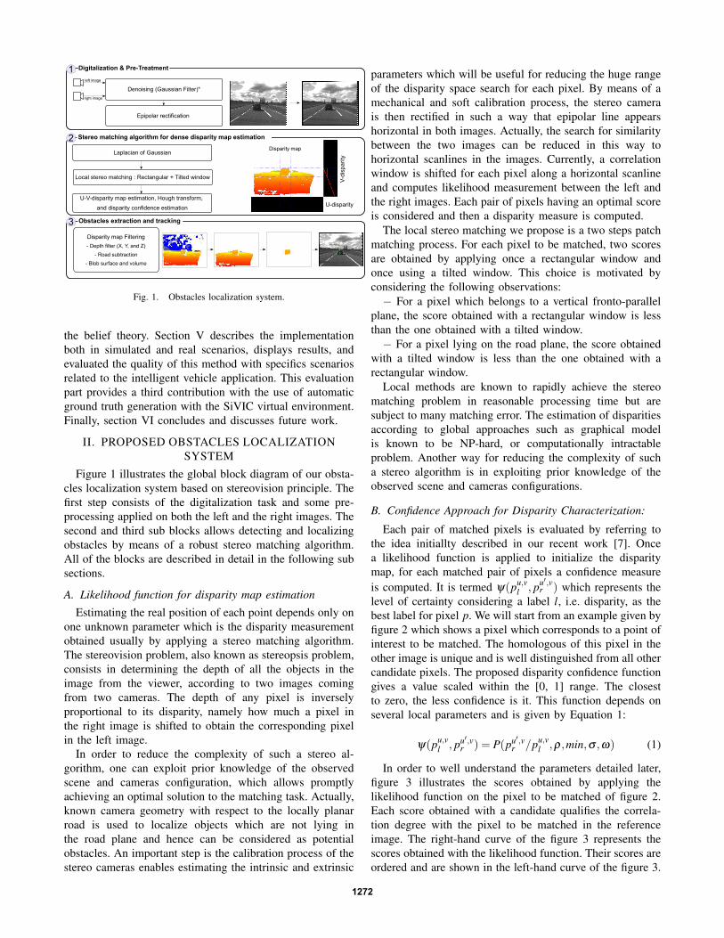
!∀#∀∃%&%
∃
∃
∀∋%(%)
∀∗
∀+∗,
−
.
/
#∀∃
!∀∃
∃
Fig. 1. Obstacles localization system.
the belief theory. Section V describes the implementation
both in simulated and real scenarios, displays results, and
evaluated the quality of this method with specifics scenarios
related to the intelligent vehicle application. This evaluation
part provides a third contribution with the use of automatic
ground truth generation with the SiVIC virtual environment.
Finally, section VI concludes and discusses future work.
II. PROPOSED OBSTACLES LOCALIZATION
SYSTEM
Figure 1 illustrates the global block diagram of our obsta-
cles localization system based on stereovision principle. The
first step consists of the digitalization task and some pre-
processing applied on both the left and the right images. The
second and third sub blocks allows detecting and localizing
obstacles by means of a robust stereo matching algorithm.
All of the blocks are described in detail in the following sub
sections.
A. Likelihood function for disparity map estimation
Estimating the real position of each point depends only on
one unknown parameter which is the disparity measurement
obtained usually by applying a stereo matching algorithm.
The stereovision problem, also known as stereopsis problem,
consists in determining the depth of all the objects in the
image from the viewer, according to two images coming
from two cameras. The depth of any pixel is inversely
proportional to its disparity, namely how much a pixel in
the right image is shifted to obtain the corresponding pixel
in the left image.
In order to reduce the complexity of such a stereo al-
gorithm, one can exploit prior knowledge of the observed
scene and cameras configuration, which allows promptly
achieving an optimal solution to the matching task. Actually,
known camera geometry with respect to the locally planar
road is used to localize objects which are not lying in
the road plane and hence can be considered as potential
obstacles. An important step is the calibration process of the
stereo cameras enables estimating the intrinsic and extrinsic
parameters which will be useful for reducing the huge range
of the disparity space search for each pixel. By means of a
mechanical and soft calibration process, the stereo camera
is then rectified in such a way that epipolar line appears
horizontal in both images. Actually, the search for similarity
between the two images can be reduced in this way to
horizontal scanlines in the images. Currently, a correlation
window is shifted for each pixel along a horizontal scanline
and computes likelihood measurement between the left and
the right images. Each pair of pixels having an optimal score
is considered and then a disparity measure is computed.
The local stereo matching we propose is a two steps patch
matching process. For each pixel to be matched, two scores
are obtained by applying once a rectangular window and
once using a tilted window. This choice is motivated by
considering the following observations:
− For a pixel which belongs to a vertical fronto-parallel
plane, the score obtained with a rectangular window is less
than the one obtained with a tilted window.
− For a pixel lying on the road plane, the score obtained
with a tilted window is less than the one obtained with a
rectangular window.
Local methods are known to rapidly achieve the stereo
matching problem in reasonable processing time but are
subject to many matching error. The estimation of disparities
according to global approaches such as graphical model
is known to be NP-hard, or computationally intractable
problem. Another way for reducing the complexity of such
a stereo algorithm is in exploiting prior knowledge of the
observed scene and cameras configurations.
B. Confidence Approach for Disparity Characterization:
Each pair of matched pixels is evaluated by referring to
the idea initiallty described in our recent work [7]. Once
a likelihood function is applied to initialize the disparity
map, for each matched pair of pixels a confidence measure
is computed. It is termed ψ(pu,vl , p
u′,vr ) which represents the
level of certainty considering a label l, i.e. disparity, as the
best label for pixel p. We will start from an example given by
figure 2 which shows a pixel which corresponds to a point of
interest to be matched. The homologous of this pixel in the
other image is unique and is well distinguished from all other
candidate pixels. The proposed disparity confidence function
gives a value scaled within the [0, 1] range. The closest
to zero, the less confidence is it. This function depends on
several local parameters and is given by Equation 1:
ψ(pu,vl , pu′,v
r ) = P(pu′,vr /p
u,vl ,ρ,min,σ ,ω) (1)
In order to well understand the parameters detailed later,
figure 3 illustrates the scores obtained by applying the
likelihood function on the pixel to be matched of figure 2.
Each score obtained with a candidate qualifies the correla-
tion degree with the pixel to be matched in the reference
image. The right-hand curve of the figure 3 represents the
scores obtained with the likelihood function. Their scores are
ordered and are shown in the left-hand curve of the figure 3.
1272

Fig. 2. An example of a point of interest to be matched from the rightimage which visibilly have one well identified correspondant in the leftimage.
(a) (b)
Fig. 3. Likelihood scores of the pixel of figure 2 obtained for each candidatepixels (a) non-ordered scores (b) ordered scores.
The confidence measurement function is given by Equa-
tion 2:
ψ(pu,vl , pu′,v
r ) =
(
1−min
ω
)τ2log(σ)
(2)
Where min is the Best Correlation Score, τ is the number
of potential candidate pixels among all of the candidates, σis the standard deviation of the disparity of the τ pixels, ωis the Gap between the τ th and (τ +1)th scores.
− Best Correlation Score (min): The output of the
likelihood function is a measure of the degree of similarity
between two pixels. Then, the candidate pixels are ranked
in increasing order according to their corresponding scores.
The couple of pixels that has the minimum score is
considered as the best-matched pixels. The lower the score,
the better the matching. The nearer the minimum score to
zero, the greater the chance of the candidate pixel to be the
actual correspondent.
− Number of Potential Candidate Pixels (τ): This parameter
represents the number of potential candidate pixels having
similar scores. τ has a big influence because it reflects
the behavior of the likelihood function. A high value of τmeans that the first candidate pixel is located either in a
uniform region or in a repetitive pattern of the image. The
lower the value of τ , the fewer the candidate pixels. If there
are few candidates, the chosen candidate pixel has a greater
chance of being the actual correspondent. Indeed, the pixel
to be matched belongs to a region with high variation of
gray component. A very small value of τ and a min score
close to zero, means that the pixel to be matched probably
belongs to a region of high gray variations.
− Disparity variation of the τ pixels (σ ): A disparity value
is obtained for each candidate pixel. For the τ potential
candidate pixels, we compute the standard deviation σof the τ disparity values. A small σ means that the τcandidate pixels are spatially neighbors. In this case, the
true candidate pixel should belong to a particular region of
the frame, such as an edge or a transition point. Therefore,
it increases the confidence measure. A large σ means that
the τ candidate pixels taken into account are situated in a
uniform gray region.
− Gap value (ω): This parameter represents the difference
between the τ th and (τ + 1)th scores given with the
dissimilarity function used. It is introduced to adjust the
impact of the minimum score.
For numerical purpose and to ensure that the function ψhas a value between 0 and 1, a few constraints are introduced.
The min parameter have not to be higher than ω . If so,
parameter ω is forced to min+1. Moreover, the log(σ) term
is used instead of σ , so as to reduce the impact of high value
of σ and obtain coherent confidence measures.
In the following, the way of estimating the parameter τis detailed. The number τ of potential candidate pixels is
deduced from all scores obtained with the local likelihood
function. The main idea is to detect major differences be-
tween successive scores. These major differences are called
main gaps. Let φ denote a discrete function which represents
all the scores given by the dissimilarity function in increasing
order. We introduced a second function denoted η , which
represents the average growth rate of the φ function. η can
be seen as the ratio of the difference between a given score
and the first score, and the difference between their ranks.
This function is defined in Equation 3:
η(φ u′,v) =φ u′,v(zm)−φ u′,v(z1)
zm − z1m ∈ L (3)
where L is the number of all candidates and φ u′,v(zm)is the mth dissimilarity cost among all scores obtained for
the pair of matched pixels (pu,v, pu′,v). zm is the rank of
the mth score. η(φ u′,v) is a discrete function that allows to
highlight the large gaps between scores. It is materialized
using Equation 4:
ξ (φ u′,v) =
∇ηu′,v
m2 if ∇ηu′,v > 0
−1 otherwise(4)
The previous function (Equation 4) is used to characterize
the major scores and is applied only in the case where the
gradient ∇ηu′,v has a positive sign. We have introduced
parameter m2 in order to penalize the candidate pixels
according to their rank. The number of candidate pixels is
given by Equation 5:
τ = argmaxm
ξ (φ u′,v) (5)
1273

Figure 4 illustrates an example of estimating the number
of potential candidate pixels τ by applying the ξ function on
the scores showed in figure 3. In this example there is only
one pixel which has a distinguished score among all scores.
This is visibly highlighted in figure 4 so that the τ parameter
corresponds to the rang of the higher value.
Fig. 4. The number of potential candidate pixels τ is given as the rank ofthe highest number obtained with the ξ function.
C. Weighted U- and V-disparity :
As detailed in section A, the likelihood function used for
estimating the disparity map is a two steps procedure. For
each step, a confidence map is obtained by applying the con-
fidence function, detailed in section B, in each matched pixel.
These confidence maps are termed the Obstacles Confidence
Map (OCM) and the Road Confidence Map (RCM). Recall
that the basic version of the so called V-disparity map is
basically obtained by cumulating all of disparity values along
lines and columns of the dense disparity map. Each point in
the V-disparity space corresponds to the sum of all disparities
along the same v image line. Figure 5 illustrates the two
cumulating spaces.
Fig. 5. (a) U- and V-disparity estimation from filtered dense disparity map(b) bounding box of an obstacle in the right image.
According to our knowledge, there is no improvement of
the V-disparity method since its inception. In our approach,
we propose a more general method which we term WV-
disparity. It is obtained starting from the dense disparity
map, the OCM and the RCM maps. Unlike the standard form
of the V-disparity, each pixel in the dense disparity map is
weighted by two confidence values as follow α×Co+β ×Cr.
The parameters Co and Cr correspond to the confidence
values given by the OCM and the RCM maps. In our
approach, a powerful tool is introduced in the formulation of
the V-disparity map by re-weighting the confidences values
with a non normalized parameters, α and β . Depending
on the application, one can give more importance to the
obstacles detection component or the road plane subtraction.
For obstacles detection, Co is more weighted than Cr by
assigning a hight value to α while a small one for β . This
allows highlighting frontal obstacles and ignore the road
plane. For road plane extraction, one can simply inverse the
weighting of α and β .
Empirically, the obtained weighted cumulative space, i.e.
WC-disparity, is more accurate than the original V-disparity.
The use of the WV-disparity and WU-disparity maps allows
to highlight obstacles lying on the road and best discriminat-
ing the most of unlikely obstacles more precisely than using
the standard version of the V-disparity method. However,
the localization of obstacles is done by exploiting the dense
disparity map and the cumulative spaces named Weignted
U- and V-disparity map. The pixels are clustered into two
classes, road and obstacles, after applying a Hough transform
on WV-disparity and WU-disparity in order to highlight
each principal line. The presence of vertical line means
the presence of a potential obstacle and the presence of
a sloped line illustrate the road profile. The v coordinate
of the intersection between the road profile and the v-axis
gives the horizon line. After the clustering step, the mean
weight obtained for all pixels representing each obstacle is
computed. This additional information is very useful for the
tracking module because of the attribution of an uncertainty
measure to each obstacle to be tracked. Figure 6 shows
the obtained WV-disparity map compared to the standard V-
disparity map.
(a) (b) (c)
Fig. 6. The basic V-disparity maps vs. the WV-disparity map. (a) densedisparity map (b) V-disparity map (c) WV-disparity map.
In order to identify the most of false alarms, we have
defined same filters such as the allowed volume depending
on the location of each obstacle. Each filter corresponds to
a condition which must be fulfilled and leading to eliminate,
1274

if possible, all of erroneous disparities and all of ambiguities
regions. A list of obstacles, i.e. target, is therefore obtained
on which a tracking procedure is applied.
III. TRACKING ALGORITHM
Once obstacles have been extracted from the two stereo
images, a multi-objects association algorithm is needed to
estimate the dynamic state of the targets and to monitor
appearances and disappearances of tracks. The position of
previously perceived objects is predicted at the current time
using Kalman Filtering. These predicted objects are already
known objects and will be denoted in what follows by Yj.
Perceived objects at the current time will be denoted by Xi.
In a general framework, the problem consists in identifying
an object designated by a generic variable X among a set
of hypotheses Yi. One of these hypotheses is supposed to
be the solution. The current problem consists in associating
perceived objects Xi to known objects Yj. Belief theory
allows assessing the veracity of Pi propositions representing
the matching of the different objects.
A basic belief allowing the characterization of a propo-
sition must be defined. This basic belief (mass mΘ(.)) is
defined in a [0,1] interval. This mass is very close to the one
used in probabilistic approach, except that it is distributed
on all the propositions of the referential of definition 2Ω =A/A ⊆ Ω= ∅,Y1,Y2, ...,Yn,Y1Y2, ...,Ω. This
referential is the power set of Ω = Y1,Y2, ...,Yn which
includes all the admissible hypotheses. These hypotheses
must also be exclusive (Yi∩Yj =∅,∀i 6= j). The masses thus
defined are called basic belief assignment and verify:
∑A⊆Ω
mΩ(A) = 1 A ∈ 2Ω, A 6=∅ (6)
The sum of these masses is equal to 1 and the mass
corresponding to the impossible case mΩ1..nXi(∅) must be
equal to 0. In order to succeed in generalizing the Demp-
ster combination rule and thus reducing its combinatorial
complexity, the reference frame of definition is limited with
the constraint that a perceived object can be connected with
one and only one known object. For example, for a detected
object, in order to associate among three known objects, the
frame of discernment is Ω = Y1,Y2,Y3,Y∗ where Yi means
that X and Yi are supposed to be the same object. In order to
ensure that the frame of discernment is really exhaustive, a
last hypothesis noted Y∗ is added. This one can be interpreted
as a target has no association with any of the tracks. In
fact each Yj represents a local view of the world and the Y∗represents the rest of the world. In this context, Y∗ means that
an object is associated with nothing in the local knowledge
set. The tracking module is designed to be a tool allowing a
temporal filtering of the set of detected targets. This allows a
spatial and temporal filtering of each obstacle. This tracking
stage also allows reducing both the false detections rate and
the missed detection rate. Previously, this approach has been
used in order to track obstacles with telemetric sensors in a
cartesian referential [8]. In this work, this approach has been
adapted to the image space.
IV. EVALUATION AND RESULTS
In this section we describe the quantitative and qual-
itative results of our proposed stereovision-based system
for detection and 3D localization of any kind of obstacles
in road environment in daytime. This evaluation stage has
been also done in both simulated and real environments.
We begin at the first time by evaluating the performances
of our algorithms by referring to a simulated dataset in
which all of disparity maps and obstacles ground truth
are available [9]. Figure 7 illustrates the Satory’s closed
loop tracks used for building images database on which the
proposed algorithm is evaluated. A lap around the Satory’s
track is 3.4 km with various geometrical configurations
such as straight segments, slight and sharp bends, and a
nonconstant road plane, i.e. with different slopes. The track
is also equipped with some guardrail. The guardrails are
considered as static obstacles are ignored for the detection
process. We considered only dynamic obstacles belonging
to the road plane. For qualitative evaluation purposes, we
need a ground truth at any time in order to get information
about the depth of any real point and the set of obstacles.
For experiments, the following parameters have been fixed:
the baseline, i.e. the distance between the two optical axis
of cameras, is 0.5 meter. The size of the optical sensor is
of 5.12×3.84 cm which corresponds to an image of size
640×480. For reducing processing time, only the quarter of
the image is processed. For the research of corresponding
pairs of pixels, the window size is fixed to 8×8. Knowing
that the sensors are positioned at 1.4 meter from the road
plane, the set of possible disparities values is up to 60. In
the following, the ability of the proposed system for detecting
obstacles in simulated and real database is demonstrated.
Fig. 7. Satory’s track used for evaluationg our algorithm on real en-vironment. A lap around the track is 3.4 km with different geometricalconfigurations.
A. Evaluation on simulated database
The performance of our algorithm is assessed by com-
paring the obtained detection results with a ground truth
generated by means of the SiVIC platform developed in
the LIVIC laboratory. This simulator allows modeling any
complex environment, sensors, and vehicles with realistic
rendering. However, it offers diverse and useful functionali-
ties such as adding gaussian or arbitrary noise or even rain or
fog on simulated images. The database we have generated is
obtained by simulating two cameras which gives left and
right images with their corresponding ground truth depth
maps and obstacles mask. Figure 8 illustrate a right image
with its corresponding disparity map and an image on which
real obstacles are identified.
1275
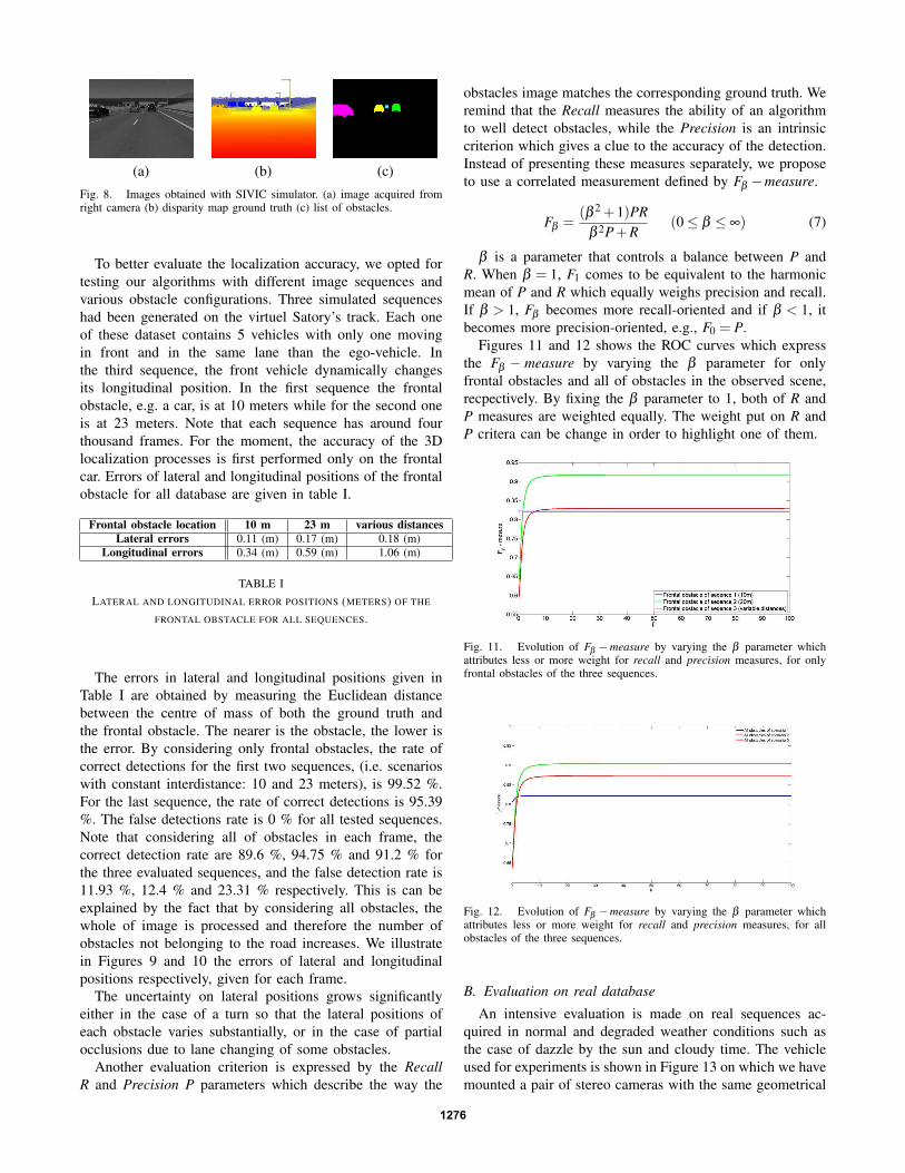
(a) (b) (c)
Fig. 8. Images obtained with SIVIC simulator. (a) image acquired fromright camera (b) disparity map ground truth (c) list of obstacles.
To better evaluate the localization accuracy, we opted for
testing our algorithms with different image sequences and
various obstacle configurations. Three simulated sequences
had been generated on the virtuel Satory’s track. Each one
of these dataset contains 5 vehicles with only one moving
in front and in the same lane than the ego-vehicle. In
the third sequence, the front vehicle dynamically changes
its longitudinal position. In the first sequence the frontal
obstacle, e.g. a car, is at 10 meters while for the second one
is at 23 meters. Note that each sequence has around four
thousand frames. For the moment, the accuracy of the 3D
localization processes is first performed only on the frontal
car. Errors of lateral and longitudinal positions of the frontal
obstacle for all database are given in table I.
Frontal obstacle location 10 m 23 m various distances
Lateral errors 0.11 (m) 0.17 (m) 0.18 (m)
Longitudinal errors 0.34 (m) 0.59 (m) 1.06 (m)
TABLE I
LATERAL AND LONGITUDINAL ERROR POSITIONS (METERS) OF THE
FRONTAL OBSTACLE FOR ALL SEQUENCES.
The errors in lateral and longitudinal positions given in
Table I are obtained by measuring the Euclidean distance
between the centre of mass of both the ground truth and
the frontal obstacle. The nearer is the obstacle, the lower is
the error. By considering only frontal obstacles, the rate of
correct detections for the first two sequences, (i.e. scenarios
with constant interdistance: 10 and 23 meters), is 99.52 %.
For the last sequence, the rate of correct detections is 95.39
%. The false detections rate is 0 % for all tested sequences.
Note that considering all of obstacles in each frame, the
correct detection rate are 89.6 %, 94.75 % and 91.2 % for
the three evaluated sequences, and the false detection rate is
11.93 %, 12.4 % and 23.31 % respectively. This is can be
explained by the fact that by considering all obstacles, the
whole of image is processed and therefore the number of
obstacles not belonging to the road increases. We illustrate
in Figures 9 and 10 the errors of lateral and longitudinal
positions respectively, given for each frame.
The uncertainty on lateral positions grows significantly
either in the case of a turn so that the lateral positions of
each obstacle varies substantially, or in the case of partial
occlusions due to lane changing of some obstacles.
Another evaluation criterion is expressed by the Recall
R and Precision P parameters which describe the way the
obstacles image matches the corresponding ground truth. We
remind that the Recall measures the ability of an algorithm
to well detect obstacles, while the Precision is an intrinsic
criterion which gives a clue to the accuracy of the detection.
Instead of presenting these measures separately, we propose
to use a correlated measurement defined by Fβ −measure.
Fβ =(β 2 +1)PR
β 2P+R(0 ≤ β ≤ ∞) (7)
β is a parameter that controls a balance between P and
R. When β = 1, F1 comes to be equivalent to the harmonic
mean of P and R which equally weighs precision and recall.
If β > 1, Fβ becomes more recall-oriented and if β < 1, it
becomes more precision-oriented, e.g., F0 = P.
Figures 11 and 12 shows the ROC curves which express
the Fβ − measure by varying the β parameter for only
frontal obstacles and all of obstacles in the observed scene,
recpectively. By fixing the β parameter to 1, both of R and
P measures are weighted equally. The weight put on R and
P critera can be change in order to highlight one of them.
Fig. 11. Evolution of Fβ −measure by varying the β parameter whichattributes less or more weight for recall and precision measures, for onlyfrontal obstacles of the three sequences.
Fig. 12. Evolution of Fβ −measure by varying the β parameter whichattributes less or more weight for recall and precision measures, for allobstacles of the three sequences.
B. Evaluation on real database
An intensive evaluation is made on real sequences ac-
quired in normal and degraded weather conditions such as
the case of dazzle by the sun and cloudy time. The vehicle
used for experiments is shown in Figure 13 on which we have
mounted a pair of stereo cameras with the same geometrical
1276

Fig. 9. The error of lateral positions (meter) for frontal obstacles: At 10m (green), 23m (blue) and variable distances (red).
Fig. 10. The error of longitudinal positions (meter) for frontal obstacles: At 10m (green), 20m (blue) and variable distances (red).
(a) (b)
Fig. 13. Overview of the proposed system (a) instrumented vehicle (b)stereovision configuration.
configuration described in the previous section. Some dozen
of sequences with four thousand images for each are used
for the evaluation.
In the database, the number of obstacles is limited to
three vehicles. We estimate that the number of obstacles
considered for the experiment is quite enough because the
road is only a two-line. Despite the use of only three
obstacles, several and various scenario are build to perform
the evaluation. The evaluated sequences are manually la-
beled while considering the correct detections, the missed
detection, and the false positives rates as a criterion for the
evaluation. For each frame, an obstacle is considered as well
detected if it is highlighted by the stereovision algorithm
relatively to the ground truth. The detection range is limited
to 5 m for the nearest obstacle and to 55 m for the farthest
one. By considering 30000 frames which are processed, the
results in terms of correct detections, missed detections, and
false detections are given in the following tables:
Correct detections Missed detections Fp
without tracking 96.49% 3.51% 2.74%
with tracking 99.04% 0.96% 0.85%
TABLE II
RATE OF CORRECT DETECTIONS, MISSED DETECTIONS AND FALSE
POSITIVES COMPUTED FOR ALL OBSTACLES.
Table II shows that the correct detections rate obtained
for the real dataset is more important that the one obtained
for simulated dataset. This can be explained by the fact that
we do not consider as obstacle both all of obstacles which
are partially overlapped by another ones and those which
1277

overtake the ego-vehicle on the left and on the right. Figure
14 shows some screenshots of the output of the stereovision
detection and tracking algorithm. The Z component of each
obstacle, i.e. how far is an obstacle from the ego-vehicle, is
displayed over each bounding box shown in green.
Fig. 14. Screenshot of some detection results obtained from real sequence.
C. Performances analysis
The proposed system has demonstrated the ability to
provide a set of relevant obstacles in daytime environment.
To be useful and in referring to the main requirement that
such a system must be embedded in a vehicle, any system
must reach the real-time performances. It is the case with
our proposed system which is first evaluated, in term of
processing time, on an Intel(R) Xeon 2.00 GHz quadruple
core processor. From all the 20 real and simulated videos
we have processed, the processing time varied between 30
and 40 ms. This time processing is lower than the sensor
sampling time (40 ms).
V. CONCLUSION
We presented comprehensive an efficient obstacle detec-
tions, 3D localization and tracking system based on stereovi-
sion principle. Results demonstrate the effectiveness of our
system in road environment. First, a dense disparity map is
estimated starting from two images. A confidence approach
is then applied for measuring the matching quality of each
pair of matched pixels. Second, a WU- and WV-disparity
maps are built which allows estimating the 2D bounding
box for each obstacle. A set of targets is then obtained
from which a tracking algorithm is applied. We note that
the main contribution of this paper is the extention and the
generalization of the V-disparity approach by weighting each
pixel in the dense disparity map for the estimation of the WV-
disparity map. Unlike the standard method, the ours offers
the possibility of highlighting either the obstacles or the road
plane. After the segmentation step, a confidence value is
attributed to each obstacle. This additional infomation is very
useful for the tracking module which makes it more robust.
The evaluation stage shows a high rate of correct de-
tections whereas a low rate of false detections and missed
detections. We have shown that most of false detections are
due mainly to the guardrail in front of the ego-vehicle in
case of sharp turn which is considered as a potential obstacle.
Missed detections mainly occurs in the case that the nearest
obstacle from the ego-vehicle is very far away (about 50m).
In this situation, the correlation window must be adapted
in order to be efficient and to allows a good enough stereo
matching. Another cause of failure in detection occurs also in
the case that two or more obstacles are at the same distance
from the ego-vehicle and are in different traffic lanes. This
leads to fuse these obstacles and the algorithm is unable to
discriminate objects really present in the disparity map. In
order to dealt with this failing, one can make dynamically
change the window size/shape for the stereo matching task.
However, the proposed approach can be applied to detect
other kind of obstacles such as pedestrian in urban scenes.
To do this, some parameters for the WU- and WV-disparity
must be adjusted.
In future work and in order to improve the current algo-
rithm, a cooperative fusion stage will be added in order to
enhance the accuracy of the obstacles localization. Reduc-
ing false negative rate and filtering out false positives can
effectively be done by merging the proposed system with a
lane markings detection module which allows identifying all
of real obstacles lying on the road. Currently, the integration
of this algorithm in a dedicated hardware architecture is in
progress.
ACKNOWLEDGMENT
The authors would like to thank the eFuture project for
funding this work. eFuture is an European IP project of the
Seventh Framework Programme (FP7).
REFERENCES
[1] D. Koller, T. Luong and J. Malik, Binocular stereopsis and lane markerflow for vehicle navigation Lateral and longitudinal control, Techni-cal Report UCB/CSD 94-804, University of California at Berkeley,Computer Science Division, 1994.
[2] L. Matthies, Stereo vision for planetary rovers : Stochastic modeling
to near real time implementation, In International Journal of ComputerVision, Vol. 8, pp. 71–91, 1992.
[3] R. Wang, Y. Xu and Y. Zhao, A vision-based road edge detection al-
gorithm, In Proceedings of the IEEE Intelligent Vehicles Symposium,Versailles, France, 2002.
[4] M. Perrolaz, J.D. Yoder, A. Negre, A. Spalanzani and C. Laugier, A
visibility-based approach for occupacy grid computation in disparity
space, In IEEE Trans. on Intelligent Transportation Systems, 2012.[5] K. Huh, J. Park and D. Hong, A stereo vision-based obstacle detection
system in vehicles, In Optics and Lasers in Engineering, Vol. 26, No.2, 2008.
[6] R. Labayrade and D. Aubert, Robust and fast stereovision based road
obstacles detection for driving safety assistance, In MVA, Nara, Japan,2002.
[7] N. Fakhfakh, L. Khoudour, J.L. Bruyelle and E. El-Koursi, Intelligent
Survellance System Based on Stereo Vision for Level Crossings Safety
Applications, In Chapter of book ’Recent Developments in VideoSurveillance’. ISBN 978-953-51-0468-1, pp. 75-100, 2012.
[8] D. Gruyer and V. Berge-Cherfaoui, Matching and decision for Vehicle
tracking in road situation, In IEEE/RSJ International Conferenceon Intelligent Robots and Systems, IROS99, Kyongju, Core, 17-21octobre 1999.
[9] D. Gruyer, S. Glaser and B. Monnier, SiVIC, a virtual platform for
ADAS and PADAS prototyping, test and evaluation, In proceeding ofFISITA10, Budapest, Hungary, 30 may-4 june 2010.
1278
The Compatibility of Energy Efficiency with Pleasure
of Driving in a Fully Electric Vehicle
Lena Rittger1 and Marcus Schmitz2
1University of Wuerzburg, Germany;
2Wuerzburg Institute for Traffic Sciences (WIVW),
Germany
Introduction
Over the past two decades there has been an increased effort in the development of
environmentally friendly mobility (Åhman, 2001; Chan, 2002; Chan & Chau, 1997; Kamal,
Mukai, Murata, & Kawabe, 2010; Neumann, Cocron, Franke, & Krems, 2010). Despite the clear
advantages of electric vehicles (e.g., higher efficiency through regenerative braking, no
emissions, more dynamic driving behaviour), the process of introducing electric vehicles to a
broad range of drivers is so far missing.
Pleasure in driving is a critical factor for the acceptance of, and attitude towards, vehicles.
The driver’s decision regarding the type of vehicle driven depends upon a number of factors,
including the positive experience and pleasure while driving (Engelbrecht, Engeln, & Arndt,
2009). The development of larger, faster, more dynamic and more comfortable vehicles for
everyday driving and to suit a broad range of buyers, supports this assumption (Dick, 2002).
The main focus of the present study was to expand research on environmentally friendly
driving and electric vehicles by applying the additional dimension of driving pleasure. The goal
was to identify driving behaviour which is energy efficient (i.e., consumes a low amounts of
energy) while at the same time is pleasant for the driver. A driver centred approach was chosen,
in which the focus of the driver as an energy optimiser who tries to improve his energy
efficiency was changed towards a view of the driver looking for pleasure and fun when driving.

Researchers have already tried to combine energy efficiency with driver acceptance (Schmitz,
Jagiellowicz, Maag, & Hanig, 2012), energy efficiency with safe driving (Fairchild et al., 2009),
and safe driving with pleasure in driving (Wedlin, Tillback, & Bane, 1992). However, this was
one of the first approaches to consider the compatibility of energy efficiency and pleasure in
driving.
Pleasure of driving
The concept of pleasure of driving has been defined in various ways in scientific and public
communication. For example, the positive emotions drivers experience when interacting with a
vehicle have, been described as physio-pleasure and psycho-pleasure (Tischler & Renner, 2007).
The former described the pleasure mediated through the sensory experience with the vehicle,
which might be comparable to a comfort component. The latter describes the pleasure arising
from the interaction with the machine and the driving action. On this background, Tischler and
Renner (2007) defined pleasure of driving as the “positive emotional state of a person, caused by
active action and determined by an actual sensory experience of the interaction of human,
vehicle, and environment” (p. 109). Using this definition, the dynamic features of the vehicle
become a crucial aspect in the examination of driving pleasure, since the dynamic operations the
driver intends to achieve directly depend on the dynamic conversion the vehicle is able to. This
means that behaviour can only be realised in between the borders of the according dynamic
values (e.g. acceleration) by which the vehicle is characterised. The vehicle offers the sense of
mastering the power and speed of the car (Hagman, 2010, p. 25), which releases the experience
of dynamic properties from the actual car.
Adding to the distinction of comfort and pleasure in driving, Engeln, Engelbrecht, and
Kieninger (2008) defined their model of joy and convenience in activities. Their framework was

based on the two axis of hedonic tone and intensity of action (i.e., arousal). Pleasant situations
can be reached when convenience and joy are high. Convenience refers to extrinsically
motivated actions and is improved by reducing the number of extrinsic acts. On the other hand,
joy is high, when an optimal level of intrinsically motivated activities is reached.
The present study focused on the pleasure of the driving experience as a result of the
experience of vehicle dynamics in longitudinal and lateral direction. As a research method, direct
questioning of non-professional drivers was chosen. This is because, in terms of the evaluation of
subjective feelings when engaged in driving a vehicle, every driver can be seen as an expert
regarding his or her own experience (Krüger, Neukum, & Schuller, 1999; Tischler & Renner,
2007).
Driving styles
In order to increase the range of dynamic experiences participants had with the electric vehicle
model, driving behaviour was defined according to different driving styles. Drivers have
different preferences, needs, motivations and safety estimations for everyday driving (Ayres, Li,
Schleuning, & Young, 2001; Hoedemaeker & Brookhuis, 1998), which result in different starts
and strengths of the dynamic reactions in various traffic situations. For example, different drivers
start decelerating in order to stop at a red traffic light at different points in time and with different
strengths of deceleration, which in consequence results in different speed profiles. Driving style
has been distinguished from driving skill. The former concerns the ability of the driver to control
the vehicle, the latter reflects the habitual mode of operating the vehicle (West, French, Kemp, &
Elander, 1993). For the classification of driving styles, various classification parameters have
been investigated, such as speed (e.g., Ebersbach, 2006), acceleration (e.g., Canale, Malan, &
Murdocco, 2002), deceleration (Tomaszewski, 2011), lateral accelerations (e.g., Neumerkel,
Rammelt, Reichardt, Stolzmann, & Vogler, 2002) and distance to the lead vehicle (Doshi &
Trivedi, 2010). These styles have been classified as part of a continuum (e.g., Ehrenpfordt, 2009)
and as distinct styles (De Vlieger, 1997). Amongst others, König, Weiß and Mayser (2002; cited
in Ebersbach, 2006) reported that the distinction of the three driving styles (i.e., sporty, normal
and relaxed) was most appropriate for the evaluation of driver assistance systems.
In the present approach, an efficient driving style was developed as an anchor for the two
driving styles of relaxed and sporty driving. It was assumed that stronger dynamic reactions (e.g.,
stronger deceleration and stronger acceleration) were associated with sporty driving behaviour,
whereas less strong dynamic reactions were associated with relaxed driving. The efficient
driving style contained components of both styles.
Method
Design
The experiment had a 3 (driving style) x 4 (driving situation) within-subject design. Every
participant experienced the three different driving styles of efficient, relaxed and sporty driving
when driving three different times on the same test track. The test track consisted of a number of
different combinations of the four main driving situations: (1) deceleration towards a lower
speed limit, (2) acceleration towards a higher speed limit, (3) curve driving and (4) car following.
The dependent variables were the energy efficiency and the pleasure drivers experienced in each
driving situation.
Apparatus
A driving simulator with a motion system based on a Steward platform with six degrees of
freedom was used in this research (Figure 1).
[insert Figure 1 here]

A vehicle and consumption model for a fully electric vehicle was implemented in the existing
simulation environment. The vehicle was equipped with an intelligent adaptive cruise control
(ACC) system. The system was able to conduct full longitudinal control, since it detects and
reacts to traffic signs, place-name signs, traffic lights, sharp corners and lead vehicles. This
ensured a consistent representation of vehicle dynamics for all participants.
Test track
The test track consisted of rural and urban areas and one inner city section. Overall the track was
24,760 metres long and included various speed changes of different velocities. The corners on
which the ACC regulated speed were always approached at a speed of 100 km/h. The two car
following situations were operated with a lead vehicle fluctuating between 60 to 80 km/h on a
rural road. Figure 2 depicts the speed profile of the track with the highlighted areas representing
inner city sections.
[insert Figure 2 here]
Parameterisation
For the realisation of dynamic behaviour, the ACC system was programmed with three sets of
parameters, representing the three different driving styles of efficient, relaxed and sporty driving.
The parameter combination of the efficient style was based on pre-tests. In the pre-tests, the
energy efficient driving style was defined according to the four types of driving situations:
deceleration, acceleration, lateral accelerations for cornering and distance to the lead vehicle.
After completing the definition of efficient driving, adaptations of the parameter combinations in
the four situations were made to simulate either a sporty or a relaxed driving style. The criteria
used were based on data from the literature and adjusted by trial and error. The final parameter
combinations for each simulated mode of driving are shown in Table 1. As can be seen, the
objective was to keep two of the three versions equal in the definition of the parameters for one

specific situation. Because of its high complexity and the interaction between the variables, this
goal could not be achieved in the car following situation, where the weighting factors for
approaching distance and the speed of the lead vehicle (kd and kv; for a more detailed
explanation see Ludmann & Weilkes, 1999), and the distance to the lead vehicle (TdistTarget)
differed between all three systems.
[insert Table 1 here]
Participants
Twenty four participants (50% female) from took part in the study. Their mean age was 36.58
years old (SD = 11.843) and they ranged in age from 25 to 59 years old. All drivers had
previously been trained for driving in the simulator, but they were not familiar with the new
electric vehicle model.
Procedure
After arriving in the laboratory, drivers completed a data privacy statement and received an
overview of the experimental structure. The ACC system and the instrument panel were
explained to the participants. After a test drive, in which participants familiarised themselves
with the dynamics of the electric vehicle and the handling of the ACC system, the simulated
ACC drives were conducted with all three driving styles in randomised order. Drivers were not
aware of the underlying parameter combinations, but were only instructed to evaluate three
versions of dynamic driving behaviour. During the drives, participants were asked two questions
in all of the relevant situations:
How strong was the driving behaviour (e.g., the deceleration)?
How pleasant was the driving behaviour (e.g., the deceleration)?
They replied on a scale from 0 (Not at all) to 15 (Very strong) and the experimenter recorded
their verbal evaluations. Drivers also had the chance to have a rest between each ACC trial. After

all the trials were completed, participants were thanked and received a compensation for
expenses.
Results
The results were analysed according to the objective energy efficiency of the drive as well as the
subjective pleasure experienced by the drivers. The ANOVAs were conducted in a repeated
measures design, and subsequent Bonferroni post-hoc tests for paired samples were reported
with adjusted alpha-levels. For the analyses, the start and the end of each single dynamic
manoeuvre were defined by the start and the end of the least dynamic system (i.e. the relaxed
ACC) for all three trials. This guaranteed that the length of the relevant sections (in which e.g. a
specific deceleration manoeuvre takes place) was the same for all systems, which is especially
crucial for the comparison of the energy efficiency.
Deceleration
In terms of energy efficiency, the three systems differ significantly (F(2,766) = 245.10, p =
.000). The relaxed system consumed less energy than both other ACC systems (relaxed vs.
efficient, p = .000; relaxed vs. sporty, p = .000), and the sporty ACC consumed less energy than
the efficient ACC (p = .000). Furthermore, the energy recuperation (i.e., the sum of all regained
energy) also differed significantly (F(2,766) = 80.793, p = .000), with all systems differing from
each other (efficient vs. relaxed, p = .000; efficient vs. sporty, p = .000; relaxed vs. sporty, p =
.000; Figure 3). This was the case, even though as intended, the efficient and the sporty versions
decelerated more strongly than the relaxed ACC (F(2,766) = 8269,1, p = .000; efficient vs.
relaxed, p = .000; efficient vs. sporty, p = .000; relaxed vs. sporty, p = .000; Figure 3).
[insert Figure 3 here]

A closer examination of the data revealed the reason for the unexpected better energy
consumption of the relaxed ACC, in comparison to the efficient system. As can be seen in Figure
4, the efficient ACC drives with a constant high speed for a longer period of time than is the case
for the relaxed ACC. Therefore, in the efficient ACC energy recuperation starts later and lasts a
shorter period of time than in the relaxed ACC. Hence, the longer recuperation period of the
relaxed ACC compensates for the fact that the maximum recuperation was not as strong
compared to the efficient ACC.
[insert Figure 4 here]
The pleasure drivers experienced in the deceleration situations differed most clearly between the
efficient and the relaxed ACC modes (F(2, 752) = 10.935, p = .000; efficient vs. relaxed, p =
.000; efficient vs. sporty, p = .021; relaxed vs. sporty, p = .022). Additionally, Figure 5 shows
that in general greater dynamic behaviour was associated with less pleasure (supported by a
significant negative correlation of r = -.349).
[insert Figure 5 here]
Acceleration
As intended, the sporty ACC version accelerated more strongly than the relaxed (p = .000) and
the efficient versions (p = .000; F(2,334) = 29554, p = .000; Figure 6). As a consequence, the
sporty ACC consumed significantly more energy than the efficient (p = .000) and the relaxed
ACC versions (p = .000; F(2,334) = 387.18, p = .000). However, when only considering the
amount of energy consumed in the acceleration manoeuvre itself, the sporty ACC consumed
significantly less energy than the other two versions (F(2,334) = 32.558, p = .000; sporty vs.
efficient, p = .000; sporty vs. relaxed, p = .000). One of the factors influencing the higher energy
consumption in the sporty version was reaching the maximum speed earlier in each situation, and
with that, a higher overall mean speed in each driving scenario. This means that in particular start

and relative speed combinations, the shorter duration of the manoeuvre compensates for the
stronger acceleration (i.e., the shorter time period leads to less energy consumption).
[insert Figure 6 here]
In the acceleration situations, no differences in pleasure were found, even though the
difference in the strength of acceleration were correctly identified by the drivers (F(2,332 =
555.05, p = .000). The sporty version of the ACC was reported to accelerate more strongly than
the efficient (p = .000) and the relaxed ACC modes (p = .000) (see Figure 7).
[insert Figure 7 here]
Cornering
Cornering was investigated as a composition of the deceleration when approaching the corner,
constant speed when driving through the corner and subsequent acceleration when exiting the
corner. The three ACC systems differ significantly in their dynamic behaviour in all three parts
of the corner (maximum deceleration F(2,190) = 867817, p = .000; minimum speed while
cornering F(2,190) = 270232, p = .000; maximum acceleration F(2,190) = 110378, p = .000;
Figure 7).
[insert Figure 8 here]
The different approaches to cornering resulted in an overall energy consumption that differed
significantly between the ACC versions (F(2,190) = 429.17, p = .000). The efficient ACC
consumed more energy than the relaxed (p = .000) and the sporty versions (p = .001), while the
relaxed mode consumed less energy than the sporty version of the ACC (p = .000). Therefore,
even during cornering the relaxed ACC had the best overall energy balance of all three ACC
modes.
Figure 8 shows the decomposed energy consumption for the three parts of a single right
hand corner. When decelerating in the approach phase of the corner, the relaxed version

regenerated more energy than the efficient (p = .000) and the sporty versions of ACC (p = .000;
F(2,46) = 16003, p = .000), which confirms the observations made during the deceleration phase
(longer deceleration compensated for the more gentle deceleration). In the steady driving phase,
higher speeds lead to higher energy consumption (F(2,46) = 11680, p = .000), meaning that the
relaxed ACC consumed less energy than the efficient (p = .000) and the sporty ACC (p = .000).
Finally, when exiting the corner the systems accelerate back to 100 km/h. Here, the relaxed
system consumed more energy than either the efficient (p = .000) or the sporty versions (p =
.000; F(2,46) = 124898, p = .000). Additionally, the sporty mode consumed more energy than
the efficient ACC (p = .000), which demonstrates that at certain relative speeds lower strength of
acceleration (and with that a longer acceleration period) is still more beneficial for energy
efficiency, compared to shorter, but stronger acceleration..
[insert Figure 9 here]
Figure 9 shows the drivers’ reported pleasure while decelerating when approaching a
corner and passing through it. The drivers’ evaluations of pleasure differed significantly between
the ACC systems (F(1,184) = 28.540, p = .000; efficient vs. relaxed, p = .000; relaxed vs. sporty,
p = .000; Figure 9).
[insert Figure 10 here]
Car following
The investigation of the dynamic driving behaviour in car following situations showed that the
intended maximum accelerations and decelerations were achieved. However, the distances to the
lead vehicle were not achieved as intended and there appeared to be inconsistencies between the
two car following situations.
The relaxed version consumed less energy than the efficient (p = .000) and the sporty
versions (p = .000), and the efficient version consumes less energy than the sporty ACC (p =

.000; F(2,94) = 1070.0, p = .000). In terms of energy recuperation, the lowest recuperation was
found in the efficient version, followed by the sporty (p = .000) and the relaxed ACC (p = .000;
F(2, 94) = 975.74, p = .000; Figure 10).
Even though drivers experienced the differences in dynamic behaviour (the relaxed version was
evaluated as decelerating and accelerating more gently than the efficient (p = .000) and the
sporty versions (p = .000), F(2,94) = 9.449, p = .000), but no differences in pleasure was found.
In general, many drivers expressed their preference for overtaking in this section of the drive,
where the speed limit was actually 100 km/h. Additionally, as the lead car fluctuated between 60
and 80 km/h closely following the speed profile of the lead vehicle was experienced as
unpleasant for drivers in all ACC versions, which was mentioned in the free comments of drivers
after the drive.
[insert Figure 11 here]
Discussion
Firstly, it can be concluded that with the described method of using an intelligent ACC system,
the goal of realising consistent driving behaviour between drivers was achieved. All drivers
experienced decelerations, accelerations and cornering in the exact same way. Additionally, the
manoeuvres were all operationalised as intended. This was important in order to guarantee a
controlled dynamic experience for drivers and to make the energy consumption values
comparable. The method of using the ACC system as a research tool was also found to be useful,
except in the car following situation, where the large number of parameters made the interactions
difficult to predict.
Secondly, the differences in the dynamic behaviour of the ACC systems were noticed by
the participants. For the large variety of dynamic experiences, drivers were able to perceive even

small differences between and within the systems. Additionally, the participants identified the
direction in which the differences had occurred. This was particularly important for the
investigation of pleasure, in that only when drivers notice differences in dynamic behaviour can
differences in pleasure can be interpreted in a meaningful way.
Thirdly, in terms of energy efficiency the hypotheses were only partially confirmed. The
relaxed ACC mode showed the most efficient driving behaviour and outperformed the efficient
and the sporty version of the ACC in terms of its energy consumption. One reason for this can be
seen in the approach of defining efficient driving behaviour on a manoeuvre level as in the pilot
research, the deceleration and acceleration manoeuvres were considered separately. However,
the sequence of manoeuvres has a major influence on efficiency. Various combinations of
dynamic behaviour and especially the consequences of present dynamic reactions for the
immediately following driving (e.g., stronger acceleration leads to reaching the target speed
earlier and driving for longer at a high speed) need to be considered in order to assure the most
energy efficient way of solving each particular situation. Also confirming this, the main reason
for the lower energy consumption in the relaxed mode was the lower mean speed the system
chose in comparison to the efficient and the sporty systems, which was caused by earlier speed
reductions and reaching the maximum speed later in each situation. Hence, the mean speed
(which was not systematically varied between systems in the present research) is one of the most
important influences on energy consumption.
Fourthly, lower vehicle dynamics resulted in higher ratings of pleasure evaluations, which
resulted in the driving behaviour of the relaxed ACC system being evaluated as the most
pleasant. In general, the pleasure evaluations were quite high, which leads to the conclusion that
none of the ACC modes were was dramatically lowering pleasure. However, differences were

observed which can be seen in relation to the differences in the experience of the vehicle
dynamics.
One factor influencing the high level of pleasure reported in the relaxed driving mode
might be the passive experience drivers had with the ACC systems. More dynamic behaviour (as
shown by the sporty and efficient system) might result in higher pleasure evaluations when
longitudinal control is actively chosen by the drivers. Regarding the definition of driving
pleasure (Tischler & Renner, 2007) the criterion of a sensory experience was reached using this
research method, whereas the criterion of applying active action did not apply for longitudinal
control. As an alternative approach, future research could try to instruct concrete driving
behaviour in order to achieve more active driving while still ensuring the comparability of the
dynamic experiences.
Finally, from the investigation of energy efficient driving and the pleasure evaluations,
driving behaviours could be identified which increased energy efficiency and driving pleasure
(Table 2). It can be concluded that energy efficiency and pleasure in driving are not contradictory
goals, but can both be achieved using the same dynamic behaviour.
[insert Table 2]
References
Åhman, M. (2001). Primary energy efficiency of alternative powertrains in vehicles. Energy,
26(11), 973-989.
Ayres, T., Li, L., Schleuning, D., & Young, D. (2001, August 25-29). Preferred time-headway of
highway drivers. Paper presented at the IEEE Intelligent Transportation Systems., Oakland
(CA) USA.

Canale, M., Malan, S., & Murdocco, V. (2002). Personalization of ACC Stop and Go task based
on human driver behaviour analysis. Paper presented at the 15th Triennial World Congress,
Barcelona, Spain.
Chan, C. (2002). The state of the art of electric and hybrid vehicles. Proceedings of the IEEE,
90(2), 247-275.
Chan, C., & Chau, K. (1997). An overview of power electronics in electric vehicles. Industrial
Electronics, IEEE Transactions on, 44(1), 3-13.
De Vlieger, I. (1997). On board emission and fuel consumption measurement campaign on
petrol-driven passenger cars. Atmospheric Environment, 31(22), 3753-3761.
Dick, M. (2002). Auf den Spuren der Motive, Auto zu fahren - Die Perspektive der Fahrenden
[Searching for the motifs of driving - the driver’s perspective]. Verkehrszeichen, 18(4), 9-16.
Doshi, A., & Trivedi, M. M. (2010). Examining the impact of driving style on the predictability
and responsiveness of the driver: Real-world and simulator analysis. Paper presented at the
Intelligent vehicle symposium (IV), IEEE.
Ebersbach, D. (2006). Entwurfstechnische Grundlagen für ein Fahrerassistenzsystem zur
Unterstützung des Fahrers bei der Wahl seiner Geschwindigkeit [Technical basis for a driver
assistance system to assist the driver in choosing the speed]. Doktorarbeit, Technische
Universität Dresden, 2006.
Ehrenpfordt, I. (2009). Zur belastungsoptimierten Routengenerierung im Straßenverkehr [Work
load optimised route generation in road traffic]: Dt. Zentrum für Luft-und Raumfahrt.
Engelbrecht, A., Engeln, A., & Arndt, S. (2009). Unterstützung von Fahrkomfort und Fahrspaß
durch Fahrerassistenzsysteme [Support for driving comfort and driving pleasure with
advanced driver assistance systems]. Paper presented at the Beiträge 8. Berliner Werkstatt
MMS, TU Berlin.

Engeln, A., Engelbrecht, A., & Kieninger, C. (2008). Joy and convenience of driving. Paper
presented at the 4th International Congress of Traffic and Transport Psychology (ICTTP),
Washington D.C.
Fairchild, R., Brake, J., Thorpe, N., Birrell, S., Young, M., Feldstead, T., & Fowkes, M. (2009).
Using on-board driver feedback systems to encourage safe, ecological and efficient
driving:The Foot-LITE Project. Paper presented at the AISB 2009 Convention: Adaptive and
Emergent Behaviour and Complex Systems, Aberdeen, Scotland.
Hagman, O. (2010). Driving Pleasure: A Key Concept in Swedish Car Culture. Mobilities, 5(1),
25-39.
Hoedemaeker, M., & Brookhuis, K. (1998). Behavioural adaptation to driving with an adaptive
cruise control (ACC). Transportation Research Part F: Traffic Psychology and Behaviour,
1(2), 95-106.
Kamal, M., Mukai, M., Murata, J., & Kawabe, T. (2010). Ecological driver assistance system
using model-based anticipation of vehicle-road-traffic information. Intelligent Transport
Systems, IET, 4(4), 244-251.
Krüger, H.P., Neukum, A., & Schuller, J. (1999). Bewertung von Fahrzeugeigenschaften – vom
Fahrgefühl zum Fahrergefühl [Assessment of vehicle characteristics - from the driving
experience to the drivers‘ experience]. VDI Bericht, 22.
Ludmann, J., & Weilkes, M. (1999). Fahrermodelle als Hilfsmittel fuer die Entwicklung von
ACC-Systemen [Driver models as a tool for the development of ACC systems]. ATZ.
Automobiltechnische Zeitschrift, 101(5).
Neumann, I., Cocron, P., Franke, T., & Krems, J. F. (2010). Electric vehicles as a solution for
green driving in the future? A field study examining the user acceptance of electric vehicles.

Paper presented at the European Conference on Human Interface Design for Intelligent
Transport Systems, Berlin, Germany.
Neumerkel, D., Rammelt, P., Reichardt, D., Stolzmann, W., & Vogler, A. (2002). Fahrermodelle
- Ein Schluessel fuer unfallfreies Fahren? [Driver models – A key for accident-free driving?]
KI, 16(3), 34-36.
Schmitz, M., Jagiellowicz, M., Maag, C., & Hanig, M. (2012). Drivers´ acceptance of limiting
vehicle dynamics in electric vehicles. 5th International Conference on Traffic and Transport
Psychology (ICTTP), Groningen, The Netherlands.
Tischler, M. A., & Renner, G. (2007). Ansatz zur Messung von positivem Fahrerleben - Die
Messung von Fahrspaß und Ableitungen für die Fahrzeuggestaltung [Approach for measuring
positive driving experience - The measurement of driving pleasure and outlets for the vehicle
design]. VDI Bericht Nr. 2015, 105-117.
Tomaszewski, M. (2011). Identifikation und Vorhersage des Fahrstils über Geschwindigkeits-
und Beschleunigungsverhalten des Fahrers [Identification and prediction of the driving style
regarding speed and acceleration behaviour of the driver]. Report. Julius-Maximilians-
Universität Würzburg. Würzburg.
Wedlin, J., Tillback, L. R., & Bane, O. (1992). Combining properties for driving pleasure and
driving safety: a challenge for the chassis engineer: Society of Automotive Engineers, 400
Commonwealth Dr, Warrendale, PA, 15096, USA.
West, R., French, D., Kemp, R., & Elander, J. (1993). Direct observation of driving, self reports
of driver behaviour, and accident involvement. Ergonomics, 36(5), 557-567.

Figure 1. Driving simulator with motion system
Figure 2. Speed profile of the test track.

Efficient Relaxed Sporty
ACC version
ど1.8
ど1.6
ど1.4
ど1.2
ど1.0
ど0.8
ど0.6
ど0.4
ど0.2
0.0Acceleration
[m/s²]
Efficient Relaxed Sporty
ACC version
ど90
ど80
ど70
ど60
ど50
ど40
ど30
ど20
ど10
0
Consumption
[Wh]
Energy consumption
Recuperated energy
Figure 3. Means (SD) of maximum deceleration (left) and energy consumption and energy
recuperation (right) in deceleration situations by ACC versions [n=24]
Figure 4. Scatterplots for speed and energy consumption while decelerating from 70 to 50
km/h for the three ACC versions [n=1]

Efficient Relaxed Sporty
ACC version
0
2
4
6
8
10
12
14
Score
[0ど15]
Dynamic score Pleasure
Figure 5. Means (SD) of scores for strength of the vehicle movements and pleasure in all
deceleration situations for the three ACC versions [n=24]
Efficient Relaxed Sporty
ACC version
0.0
0.2
0.4
0.6
0.8
1.0
1.2
1.4
1.6
1.8
Acceleration
[m/s²]
Efficient Relaxed Sporty
ACC version
0
40
80
120
160
200
240
280
Consumption
[Wh]
Overall situation Acceleration manoeuvre
Figure 6. Means (SD) for maximum acceleration (left), overall energy consumption and in
the acceleration process (right) for the three ACC versions [n=24]
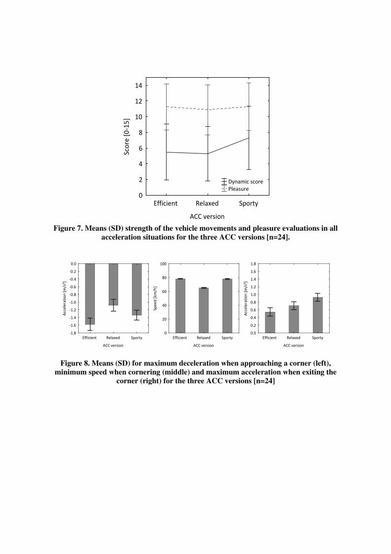
Efficient Relaxed Sporty
ACC version
0
2
4
6
8
10
12
14
Score
[0ど15]
Dynamic score Pleasure
Figure 7. Means (SD) strength of the vehicle movements and pleasure evaluations in all
acceleration situations for the three ACC versions [n=24].
Efficient Relaxed Sporty
ACC version
ど1.8
ど1.6
ど1.4
ど1.2
ど1.0
ど0.8
ど0.6
ど0.4
ど0.2
0.0
Acceleration
[m/s²]
Efficient Relaxed Sporty
ACC version
0
20
40
60
80
100
Speed
[km/h]
Efficient Relaxed Sporty
ACC version
0.0
0.2
0.4
0.6
0.8
1.0
1.2
1.4
1.6
1.8
Acceleration
[m/s²]
Figure 8. Means (SD) for maximum deceleration when approaching a corner (left),
minimum speed when cornering (middle) and maximum acceleration when exiting the
corner (right) for the three ACC versions [n=24]

Efficient Relaxed Sporty
ACC version
ど120
ど100
ど80
ど60
ど40
ど20
0
Consumption
[Wh]
Efficient Relaxed Sporty
ACC version
0
20
40
60
80
100
120
Consumption
[Wh]
Efficient Relaxed Sporty
ACC version
0
20
40
60
80
100
120
Consumption
[Wh]
Figure 9. Means (SD) of fuel consumption for approaching the corner (left), cornering
(middle) and leaving the corner (right) for the second sharp right corner [n=24]
Efficient Relaxed Sporty
ACC version
0
2
4
6
8
10
12
14
Score
[0ど15]
Dynamic score approach Pleasure approach Pleasure pass through
Figure 10. Means (SD) for the strength of the deceleration and pleasure when approaching
the four corners and cornering in the three ACC versions [n=24]

Efficient Relaxed Sporty
ACC version
0
20
40
60
80
100
120
140
160
Consumption
[Wh]
Efficient Relaxed Sporty
ACC version
ど160
ど140
ど120
ど100
ど80
ど60
ど40
ど20
0
Consumption
[Wh]
Figure 11. Means (SD) for overall energy consumption (left) and energy recuperation
(right) in the car following situations for the three ACC versions [n=24]

Table 1. Parameters for the three ACC versions in the four different driving situations
Situation Parameter
Efficient
ACC
Relaxed
ACC
Sporty
ACC
Deceleration Max. torque limit 1550 Nm 200 Nm 1550 Nm Max. power limit 25 kW 10 kW 25 kW
Acceleration Max. torque limit 700 Nm 700 Nm 1550 Nm Max. power limit 12.5 kW 12.5 kW 25 kW
Curves Max. lateral acceleration
3.2 m/s² 2.2 m/s² 3.2 m/s²
Car following kd 0.1 0.5 2.0 kv 0.1 0.1 0.8 TdistTarget 2.0 s 3.0 s 1.3 s
Table 2. Factors increasing energy efficiency and driving pleasure in the present electric
vehicle
Situation Increasing energy efficiency Increasing pleasure
Deceleration Earlier deceleration and longer recuperation times to compensate for more gentle deceleration
More gentle and early decelerations
Acceleration Lower acceleration and subsequently shorter times spent with high speed positively influence energy consumption.
Pleasure is not decreased by more gentle acceleration.
Curves More gentle and longer deceleration when approaching corners, lower speeds when cornering (but only if subsequent acceleration time is not substantially increased), more gentle acceleration when leaving the corner.
More gentle deceleration when approaching corners, lower speeds when cornering.
Car following More gentle acceleration and decelerations when adapting speed.
Possibility of overtaking; if not possible, longer following distances that do not closely imitate lead vehicle’s behaviour.
The impact of different pedal solutions for supporting efficient driving with electric vehicles
Marcus Schmitz, Monika Jagiellowicz, Christian Maag, Michael Hanig
Wuerzburg Institute for Traffic Sciences (WIVW)
Raiffeisenstraße 17, 97209 Veitshoechheim, Germany
ABSTRACT:
The functionality of an electric vehicle enables to regenerate energy into the battery by using the electric motors for electric braking. By integrating this electric brake into the accelerator pedal, drivers are expected to use more often the electric brake and less often the hydraulic brake. However, the pedal system of a car is a crucial connection between driver and car. Any modification of this part can lead to decreasing acceptance. A driving simulator study was conducted to investigate the impact of this combined pedal solution (CPS) on acceptance and energy consumption. 24 participants performed test drives in rural and urban environment with both, the CPS and a conventional pedal solution. With the CPS, drivers used less often the hydraulic brake. This behaviour led to less energy consumption. Additionally, using the CPS resulted in higher subjective ratings due to the comfort of managing most traffic situations with only one pedal.
1 Introduction
One key feature of an electric vehicle is the partitioning between the electric
and the hydraulic brake force. This fact makes it possible to combine
accelerating and electric braking on the accelerator pedal (combined pedal
solution (CPS)). Another more conventional solution is to implement the
electric brake into the hydraulic brake pedal and thus split up braking
completely from the accelerator (split pedal solution (SPS)). The CPS can be
understood as an “augmentation of existing in-car interfaces” [1], because
drivers can use it without the necessity of further changes of the pedal
system. The idea behind this solution is simple: by integrating the electric
brake into the accelerator pedal, drivers can use the regenerative brake force
to decelerate the car similar to the drag torque of a conventional combustion
engine. As regenerative brake forces can even be higher than the drag

torque, drivers are expected to manage most deceleration manoeuvres with
regenerative braking. Former research showed that such consequent usage
of the regenerative braking has a significant positive impact on the overall
energy consumption [2]. Thus, the CPS supports the driver in avoiding
energy losses by braking hydraulically. However, the pedal system of a car is
a crucial and safety-critical connection between driver and car. Any
modification of this part could negatively influence the driving performance in
terms of safety and usability. This paper describes a study that determined
the impact of the CPS in comparison to the SPS on both the driver’s
acceptance and the energy consumption. In addition, frequency and duration
of hydraulic brake pedal usage were recorded and examined.
2 Method
2.1 Pedal configurations
Figure 1 illustrates the pedal configurations of the CPS (left) and the SPS
(right). The braking pedal of the CPS remains reserved for the hydraulic
brake only. The electric brake is set on the first 20 % of the accelerator pedal
way; accelerating starts at 30 %. The sailing area (i.e. neither acceleration
nor braking) lies between electric braking and acceleration (i.e. between 20-
30 % of pedal way). The vehicle brakes with maximum electric brake forces
when neither the accelerator pedal nor the brake pedal is pressed.
0%
100%
Hydraulic
brake
0%
100%
20%
30%Sailing
Electric
brake
Acceleration
Combinedpedal solution
Split pedal solution
0%
100%
20%Electric
brake
Hydraulic
brake
0%
100%
Acceleration
Figure 1. Configuration of brake pressure and accelerator pedal way for
CPS (left) and SPS (right)
The SPS integrates the electric brake into the first 20 % of the brake pedal
pressure and the hydraulic brake between 80-100 %. The accelerator pedal
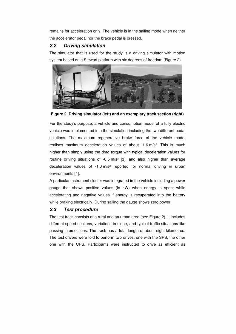
remains for acceleration only. The vehicle is in the sailing mode when neither
the accelerator pedal nor the brake pedal is pressed.
2.2 Driving simulation
The simulator that is used for the study is a driving simulator with motion
system based on a Stewart platform with six degrees of freedom (Figure 2).
Figure 2. Driving simulator (left) and an exemplary track section (right)
For the study’s purpose, a vehicle and consumption model of a fully electric
vehicle was implemented into the simulation including the two different pedal
solutions. The maximum regenerative brake force of the vehicle model
realises maximum deceleration values of about -1.6 m/s². This is much
higher than simply using the drag torque with typical deceleration values for
routine driving situations of -0.5 m/s² [3], and also higher than average
deceleration values of -1.0 m/s² reported for normal driving in urban
environments [4].
A particular instrument cluster was integrated in the vehicle including a power
gauge that shows positive values (in kW) when energy is spent while
accelerating and negative values if energy is recuperated into the battery
while braking electrically. During sailing the gauge shows zero power.
2.3 Test procedure
The test track consists of a rural and an urban area (see Figure 2). It includes
different speed sections, variations in slope, and typical traffic situations like
passing intersections. The track has a total length of about eight kilometres.
The test drivers were told to perform two drives, one with the SPS, the other
one with the CPS. Participants were instructed to drive as efficient as

possible by keeping to three advices: use the hydraulic brake as little as
possible, sail as often as possible and try not to enter the highest “red area”
of the power gauge when accelerating (i.e. >40 kW). After the first and the
second ride participants were asked two questions answered by means of a
15 point category subdivision scale:
What do you think, how successful have you been in driving energy
efficiently? (not at all – very successful)
How suitable is the pedal solution for driving energy efficiently? (not at all – very suitable)
At the end of the two drives participants were briefly interviewed. They had
the possibility to answer how they liked the two pedal solutions, which pedal
solution they would prefer and why.
2.4 Participants
24 Participants were recruited from the WIVW test driver panel. All drivers
had been trained for the simulator and had taken part in at least one driving
simulator study before. There were 14 men and 10 women. Mean age was
35 (sd=10) years. Mean driving experience was 15 (sd=9) years. Mean
kilometres driven per year were 16854 (sd=13700) kilometres.
3 Results
3.1 Pedal usage
The pedal solution clearly influences the way how subjects use the two
different braking modes. Driving with the CPS leads to hardly any usage of
the hydraulic brake. 10 out of 24 subjects even managed to drive the total
route without any hydraulic braking compared to none with SPS. In contrast,
driving with the SPS resulted on average in 15.3 times of braking with the
hydraulic brake (t(23)=8.77; p<.001; Figure 3 left). No effect could be found
in the mean frequency of the electric braking usage considering the total
route (t(23)=-1.96; p<.062; Figure 3 right). Having a look on the rural and
urban area separately, the electric brake is used more frequently in urban
areas in the CPS condition compared to the SPS condition (t(23)=-3.36;
p=.003). This is presumably due to more frequent changes between sailing
and electric braking during stopping manoeuvres.
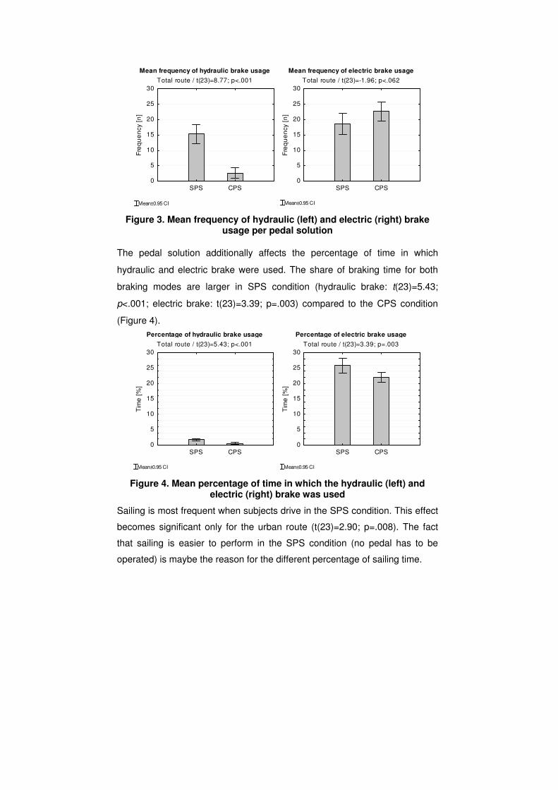
Mean frequency of hydraulic brake usage
Total route / t(23)=8.77; p<.001
SPS CPS
0
5
10
15
20
25
30
Fre
qu
en
cy [
n]
Mean±0.95 CI
Mean frequency of electric brake usage
Total route / t(23)=-1.96; p<.062
SPS CPS
0
5
10
15
20
25
30
Fre
qu
en
cy [
n]
Mean±0.95 CI Figure 3. Mean frequency of hydraulic (left) and electric (right) brake
usage per pedal solution
The pedal solution additionally affects the percentage of time in which
hydraulic and electric brake were used. The share of braking time for both
braking modes are larger in SPS condition (hydraulic brake: t(23)=5.43;
p<.001; electric brake: t(23)=3.39; p=.003) compared to the CPS condition
(Figure 4).
Percentage of hydraulic brake usage
Total route / t(23)=5.43; p<.001
SPS CPS
0
5
10
15
20
25
30
Tim
e [
%]
Mean±0.95 CI
Percentage of electric brake usage
Total route / t(23)=3.39; p=.003
SPS CPS
0
5
10
15
20
25
30
Tim
e [
%]
Mean±0.95 CI Figure 4. Mean percentage of time in which the hydraulic (left) and
electric (right) brake was used
Sailing is most frequent when subjects drive in the SPS condition. This effect
becomes significant only for the urban route (t(23)=2.90; p=.008). The fact
that sailing is easier to perform in the SPS condition (no pedal has to be
operated) is maybe the reason for the different percentage of sailing time.

3.2 Subjective ratings
There was a significant effect of pedal solution on the subjective rating on
how efficient drivers were during the drive (t(23)=6.59; p<.001). Driving with
the CPS made the drivers believe that they were driving more energy
efficiently compared to the SPS condition (Figure 5 left).
Self ev aluation of efficient driv ing
performance
t(23)=-6.59; p<.001
SPS CPS
0
2
4
6
8
10
12
14
Su
bje
ctive
ra
tin
g [
0..
.15
]
Mean±0.95 CI
Suitability of pedal solution for efficient
driv ing
t(23)=-9.04; p<.001
SPS CPS
0
2
4
6
8
10
12
14
Su
bje
ctiv r
atin
g [
0..
.15
]
Mean±0.95 CI Figure 5. Mean rating of own efficient driving performance (left) and of
adequacy of pedal solution for efficient driving (right)
Further, drivers rated the CPS as significantly more usable for driving energy
efficiently than the SPS (t(23)=9.04; p<.001, Figure 5 right).
When asking which pedal solution drivers would prefer 23 out of 24 replied
CPS. In the majority of cases the reasons were:
CPS more comfortable, since no usage of brake pedal is needed
anymore.
Easier to regenerate energy, since the power gauge delivers exact
information. The SPS lacks a gauge which delivers exact information
whether the car brakes electric or hydraulic.
Points of criticism of the CPS were:
Whilst driving with the SPS the area of sailing was much easier to
find (i.e. neither stepping on the brake nor on the accelerator pedal)
When driving with the CPS many glances to the gauge are needed in
order to obtain information whether the car is sailing, accelerating, or
regenerating energy.
3.3 Consumption measures
The subjective ratings were confirmed by the actual energy consumption.
Considering mean energy consumption, analysis revealed a significant effect

of pedal solution (t(23)=6.84; p<.001). Using the CPS results in about six per
cent less energy consumption compared to the SPS as depicted in Figure 6.
A significant effect of pedal solution can be found in the rural as well as in the
urban section.
Mean consumption per pedal solution
Total route / t(23)=6.84; p<0.001
SPS CPS
0
200
400
600
800
1000
1200
1400
En
erg
y [
Wh
]
Mean±0.95 CI Figure 6. Mean consumption (in sum) per pedal solution (total route)
This effect of the pedal solution on the overall consumption is a consequence
of significant more recuperation in the CPS condition (t(23)=7.34; p<.001). In
average, more than 100 Wh more are recuperated during the CPS mode
(Figure 7 right). This exceeds clearly the difference in the retrieved energy
from the battery that is slightly higher in CPS condition (Figure 7 left).
Spent energy per pedal solution
Total route / t(23)=1.96; p<0.062
SPS CPS
0
200
400
600
800
1000
1200
1400
1600
1800
En
erg
y [
Wh
]
Mean±0.95 CI
Recuperated energy per pedal solution
Total route / t(23)=7.34; p<0.001
SPS CPS
-500
-400
-300
-200
-100
0
En
erg
y [
Wh
]
Mean±0.95 CI Figure 7. Retrieved (left) and recuperated (right) energy (in sum) per
pedal solution (total route)

4 Discussion
The study compared the SPS with the CPS to obtain knowledge about
acceptance, vehicle dynamics and consumption issues. Drivers clearly prefer
the CPS over the SPS. Furthermore, drivers assume to drive more efficiently
when using the CPS compared to the SPS. This confirms the impression that
participants felt confident with the combined pedal solution and would even
like to use the system frequently. Similar results were found in the UC Davis
MINI E Consumer Study [5].
The CPS also changed drivers’ behaviour. By using the hydraulic brake less
often, less energy was needed. Accordingly, CPS led to a more efficient
driving behaviour compared to the SPS. However, while using CPS drivers
complained about the need to look quite often at the power gauge in order to
know whether the vehicle is accelerating, decelerating or sailing. As an
alternative feedback channel, an active accelerator pedal could be a
supporting feature providing continuous feedback about the current pedal
position.
Additional research should address the impact of the changed driving
behaviour on surrounding traffic (e.g. following vehicles). Another issue to be
investigated are long term effects of using the CPS as it has to be
guaranteed that the driver could still use the hydraulic brake quickly and
safely in non-routine (i.e. safety-critical) situations.
Acknowledgment: The study was conducted in the frame of the eFuture
project [6] that is partially funded by the European Commission under FP7.
References:
[1] Meschtscherjakov, A., Wilfinger, D., Scherndl, T. & Tscheligi, M.
Acceptance of future persuasive in-car interfaces towards a more economic
driving behaviour. AutomotiveUI 2009, Essen, Germany, Sep 2009, pp. 81–
88
[2] Walsh, C., Carroll, S., Eastlake, A. & Blythe, P. Electric Vehicle Driving
Style and Duty Variation Performance Study, 2010, Available from:
http://www.nichevehiclenetwork.co.uk/LinkClick.aspx?fileticket=WTmGSFXB
8qA%3d&tabid=531, accessed April 2012
[3] Watanabe, T. N., Kishimoto, N., Hayafune, K. & Yamada, K. Development
of an Intelligent Cruise Control System. Proceedings of the World Congress

on Intelligent Transport Systems, 1995, 3, pp. 1229-1235
[4] Hackenberg, U. & Heißing, B. Die fahrdynamischen Leistungen des
Fahrer-Fahrzeug-Systems im Straßenverkehr. ATZ Automobiltechnische
Zeitschrift, 1982, 84(7), pp. 341–344
[5] Turrentine, T., Garas, D., Lentz, A. & Woodjack, J. The UC Davis MINI E
Consumer Study. Research report UCD-ITS-RR-11-05, 2011
[6] http://www.efuture-eu.org, accessed February 2012

EVS27 International Battery, Hybrid and Fuel Cell Electric Vehicle Symposium 1
EVS27 Symposium
Barcelona, Spain, November 17-20, 2013
A safe Torque Vectoring function for an electric vehicle
Volker Scheuch, Gerd Kaiser, Matthias Korte, Peter Grabs, Fabian Kreft, Frédéric Holzmann
Corresponding author: Volker Scheuch ([email protected])
Intedis GmbH & Co.KG, Max-Mengeringhausen-Straße 5, D – 97084 Würzburg
Short Abstract
A safe Torque Vectoring function is applied to an electric vehicle with a two front motors drivetrain
concept. The function has been embedded in a lean and scalable functional architecture adaptable to
various drivetrain concepts. The Torque Vectoring function comprises an LPV control algorithm with good
performance even in extreme test cases. The controller can be parameterised for case specific performance.
The implementation of functional safety requirements is presented for one safety goal.
1 Introduction
The application of an advanced Torque Vectoring System (TorVec, TVS) to a two front motor electric
vehicle is presented. The choice of a two motor drivetrain is a reasonable compromise between a four
wheel motor approach which is complex and expensive and a conventional single motor drive with no
freedom of driving wheels individually. However, the advantages of an individual torque control on the
wheels (i.e. torque vectoring) must exceed the disadvantages by the extra costs and the extra effort for the
higher complexity (package space, weight, number of parts). This benefit for the driver first must be
carefully developed and then clearly communicated as a unique selling point for the car manufacturer to
enter the market with electric vehicles.
The results in this article will be presented for the two front motor drivetrain configuration but can be
extended to arbitrary multi wheel drives. An alternative to use two motors can be one central motor
combined with an active electric differential. This solution also suffers from extra costs and package and
compared to the use of two individual motors the dynamic range is limited by the maximum differential
ratio of torque transmission.
The advantages of a Torque Vectoring function are multiple. The first benefit arises by the mandatory need
to have a differential function for a two motor drive to compensate for different wheel speeds in cornering
situations. This principle can be used to support the steering request of the driver by a torque increase of the
outer and a torque decrease of the inner wheel. This results in a lower steering force and is equivalent to the
effect of a power steering system.
The option of automatic steering can also be used for supporting modern advanced driver assistances
systems (ADAS) functions like Lane Keeping Assistance Systems (LKAS). After identifying the lane
markings, these systems keep the vehicle in the track by controlling the yaw rate via an electric steering
system. For small road curvatures, like on highways, this could also be achieved by the asymmetrical
application of torque by a TVS.
Beside comfort applications like the above mentioned the largest benefit of TorVec is the safety aspect. In
contrast to stabilising assistance systems like electronic stability control (ESC) or antilock braking systems (ABS) which are effective by braking individual wheels, TorVec is able to support this functionality by
applying less positive or negative torque instead of using the hydraulic brakes. This benefit is experienced
by the driver in situations where an increasing wheel slip could lead to an unstable condition. Before ESC

EVS27 International Battery, Hybrid and Fuel Cell Electric Vehicle Symposium 2
would be engaged, TorVec is able to smooth out the wheel slip by reducing or increasing the torque
accordingly. Examples of these situations are laterally different friction coefficients (e.g. dry asphalt on the
left and ice on the right; “µ-split”) or oversteer / understeer. Here, TorVec extends the capability of ESC to
the very onset of these slip phenomena.
The different regimes of the assistance systems are shown in figure 1. The borders between the validity
regions are drawn sharp but will smooth out in the future when one master dynamics controller is capable
of stabilising the vehicle in both lateral and longitudinal direction. This controller must be able to drive the
hydraulics brakes, the individual electric motors, and the steering system to have maximum flexibility and
redundancy.
Figure 1: Regime of TorVec as the interfacing function between other stabilising functions. The borders could smooth
out in the future by merging the functions to a master dynamics controller. ESC = electric stability control, ABS =
antilock braking system, TCS = traction control system.
The TVS has been embedded into a new functional architecture as the link between the execution layer and
the command layer [1, 2]. This architecture approach aims at a safe and efficient operation of the EV. The
distinct separation of tasks is an important presumption for the scalability and flexibility of the concept.
One major goal in the eFuture project was to support the Functional Safety requirements with a clearly
arranged topology of the architecture and to ensure that all safety related functions – like TorVec – will
have an easy and transparent dependency from other functions which are also easy controllable.
The paper demonstrates a technical deployment of a safe drivetrain architecture for an electrical vehicle.
The implementation of the main safety requirements as prerequisites for the integration of dynamical
stability functions is shown. The approach of a LPV controller for Torque Vectoring is described and
examples for the performance of the assistance function are given.
The work is supported by the European Commission in the project eFuture [3] (grant no. 258133). The aim
is to demonstrate innovative functions embedded in a flexible and lean architecture to support safe and
efficient electric driving.
2 Functional architecture
The complexity of automotive architectures grew constantly through the last decades. The demand for safer
cars, driver assistances, and car multimedia led to new components and functions requiring an increased
number of interfaces, cables and control units with the corresponding software. This evolution, in turn,
results in a confusing system of interconnected devices and functions which hampers the introduction of
new features.
New vehicle generations offer the opportunity to think new ways for relieving this situation by modular
approaches to account for different markets and vehicle types, and to ease the integration of future
technology. The electro mobility age with its new use cases and new vehicle requirements enables the
development of innovative architectures with reduced complexity and higher sustainability.
By defining a modular and flexible architecture for a full electric vehicle (FEV), the project eFuture
translates this challenge into a demonstration car to examine the feasibility, the limits and the benefits of a
“revolution” in E/E architecture. The top level picture of the approach basically consists of four layers and
is shown in figure 2.

EVS27 International Battery, Hybrid and Fuel Cell Electric Vehicle Symposium 3
The perception layer collects all information of the vehicle’s environment via exteroceptive sensors and the sensor fusion extracts the relevant information for the guiding ADAS function on the command layer. The
driver with his senses is part of the perception layer but could also be attributed to the command layer as he
performs the transition of perception to driving commands.
The human machine interface (HMI) is split into the two directions “driver to vehicle” and “vehicle to driver” which is advantageous for the modular implementation of new driver actuators (control buttons,
pedals, etc.) and new driver feedback devices (displays, acoustic senders) and enables an easy adjustment
of the driver’s look-and-feel.
Both the HMI (driver-to-vehicle in this case) and the guiding ADAS (ACC, LKAS, EBS, etc.) are
calculating motion requests consisting of the longitudinal acceleration and the steering angle. The requests
are forwarded to a central control function, the Decision Unit 1 (DU1) which mitigates between the
potentially conflicting motion requests [1, 2]. The DU1 also receives information on the energy status of
the vehicle via the Energy Management function on the energy layer. According to the recommendation of
the Energy Management, the DU1 can choose a limitation for acceleration and/or velocity avoiding an
excessive current which could damage the high voltage battery.
The DU1 selects the best motion vector in terms of efficiency and safety and forwards this to the execution
layer, responsible for choosing the best way to realise the motion vector by the actuators present in the
vehicle (brakes, motors, active steering). The implementation of a Torque Vectoring function enables the
dynamical split of torque required for the requested acceleration to the drive wheels. Together with the
conventional stabilising ADAS (ESC, ABS, TCS), TorVec ensures safe and comfort driving in all
situations. This will be addressed in section 3.
An important part of the execution layer for the perception of the dynamical vehicle status is the Vehicle
Observer (VehObs). This function examines information of the various vehicle sensors (wheel speed
sensors, yaw rate sensor, steering wheel sensor and acceleration sensor), improves their signal quality by
the use of Extended Kalman filtering, and calculates immeasurable quantities out of the primary signals [4].
The VehObs is the source of information on dynamical vehicle stability and its limits for all functions in
this architecture.
The concept of the decision unit has also been applied to the execution layer by implementing a central
control function, the Decision Unit 2 (DU2), which decides, based on the inputs of the energy management
(recuperation en-/disabled, current limitation) and the VehObs (dynamical limits), which actuator shall
perform the requested action to achieve the requested trajectory. Here, the steering can be done by TorVec
or Power Steering, and deceleration can be performed by recuperation or hydraulic braking.
The philosophy of the novel functional architecture is to decouple the core functions from the hardware
(HW) and to create interfacing functions to the HW which can easily be adapted to different HW concepts
(e.g. drivetrain architectures, ADAS equipment, degree of autonomous driving). This concept also avoids
bypassing of functions by applying a hierarchic composition with the decision units being the final
instance.
In chapter 4 the use of this modularity for the implementation of important safety requirements from the
functional safety concept will be outlined. High ASIL ratings can be restricted to the core functions which
only carry simple calculations and thus, can easily be secured by redundancies.

EVS27 International Battery, Hybrid and Fuel Cell Electric Vehicle Symposium 4
Figure 2: Top level schematics of the functional architecture used in the eFuture project
3 Control strategy and performance of Torque Vectoring
To use a Torque Vectoring System (TVS) a special vehicle configuration must be given. In the project
eFuture the vehicle is equipped with two independent electric motors which drive the front wheels of a
compact car – as shown in figure 3.
Figure 3: eFuture propulsion system
With the two electric motors, the lateral dynamics of the vehicle can be influenced and the control of the
two motors is called torque vectoring. TVS is considered as a performance enhancement function which
also improves the vehicle stability and thus, the safety of the vehicle. In normal, every-day driving
conditions, the vehicle movement can be described with the nonlinear single track model [5]
Here the vehicle states are the longitudinal velocity 懸掴, the lateral velocity 懸槻 and the yaw rate 閤岌 . The
system inputs are the total longitudinal force デ繋掴, the front wheel steering angle 絞 and the yaw moment 警佃. Geometrical properties of the vehicle are included as distance 欠怠 which is the length between the front
axle and the centre of gravity (CoG) and the variable 欠態 which is the distance between the rear axle and the
CoG. The vehicle mass is given as 兼 and the vertical moment of inertia is given as 荊佃. The parameters 系底捗
and 系底追 represent the cornering stiffness of the front and rear axle, respectively.

EVS27 International Battery, Hybrid and Fuel Cell Electric Vehicle Symposium 5
In critical driving situations including icy road, vehicle spinning or wheel spin / blocking, the real vehicle
behaviour is different from the nonlinear single track model. With unknown and unpredictable vehicle
behaviour, most drivers are overstrained and cannot safely operate the vehicle. Torque Vectoring tries to
keep the real driving behaviour as close as possible to the normal driving behaviour reflected by the above
equations. Therefore the two electric motors at the front wheels are used to generate a total longitudinal
force デ繋掴, which accelerates and brakes the vehicle. Additionally, the motors are used to generate the yaw
moment 警佃 which controls the lateral movement of the vehicle.
The control of the vehicle dynamics can be realised with different controller types [6, 7]. For the
application in eFuture a linear parameter-varying (LPV) control design is chosen as Torque Vectoring
controller. In LPV control linear time invariant (LTI) design concepts are applied to a certain class of non-
linear systems [8]. The non-linear single track vehicle model fits perfectly the requirements of LPV control
because the non-linearity of the system can be included into the controller design. With LPV control, it is
possible to design a controller which guarantees stability over the complete operation range while
maintaining the vehicle performance [9] – which can only be guaranteed for PID controllers with an
unfavourable controller performance.
Besides the LPV controller, a torque and slip limiter (TSL) is included in the software which deals with the
physical limitations of the actuators. TSL is composed of two elements.
1. An anti-windup configuration which deals with the physical limitations of the electric drivetrain.
The power limitation introduced with the battery and the torque limitations related to the electric
motor decrease the performance of the controller as soon as the physical limitations are reached.
The anti-windup scheme [10] reduces the effects of the limitations and suppresses excessive
overshoots and vehicle instability due to actor limitations.
2. The anti-windup scheme is enhanced to TSL because it also limits the tyre slip. Excessive slip
values which represent spinning or blocking of the wheels have negative effects on the vehicle
performance and safety. To suppress these events, TSL monitors the wheel slip and keeps it in the
defined boundaries. In the actual configuration TSL does not perform any action until the tyre slip
leaves the interval [-0.1 ; +0.1]. If the tyre slip exceeds these limits the driving torque is reduced
towards zero to suppress spinning or blocking of the wheel.
The final control architecture is given in figure 4 with a desired value generator which uses the steering
angle and acceleration request of the driver to calculate a velocity request and a yaw rate request. A similar
scheme is used by [11] and shows satisfying results. The LPV controller controls the longitudinal velocity
and the yaw rate with the two electric motors. The TSL is idle if moderate requests are performed. If the
limits of the electric drivetrain or tyre slip are reached the TSL gets activated and reduces the torque
requests of the controller in order to stabilize the control-loop and thus, the vehicle.
Figure 4: Torque Vectoring control architecture
In eFuture the vehicle movement is simulated with a 14 degree of freedom model, including a linear
suspension model and a Pacejka tyre model [12]. This model is used to simulate the vehicle behaviour and
to tune the TorVec control parameters. In order to validate the controller the following test cases are
simulated:
• Straight line acceleration
• Straight line braking (ISO 21994)
• Constant radius turning (ISO 4138)
• Brake in bend (ISO 7975)

EVS27 International Battery, Hybrid and Fuel Cell Electric Vehicle Symposium 6
• Acceleration in a bend
• Step steer (ISO 7401)
• Lift off oversteer (ISO 9816)
• Sine with dwell (NHTSA [13], for ESC effectiveness)
In order to validate the lateral performance the National Highway Traffic Safety Administration (NHTSA)
advises to use a sine-with-dwell manoeuvre [13]. This test should be used to evaluate the lateral
performance of a vehicle and especially the functionality of an ESC system because an average vehicle gets
unstable in this test. Here the same test is applied to test the lateral performance of Torque Vectoring. In the
sine-with-dwell manoeuvre, the steering wheel is turned in a sinusoidal movement with a maximum angle
of 120° at the steering wheel. At the second maximum the steering wheel is kept constant for 0.5 seconds.
This manoeuvre is an open-loop manoeuvre which means that no real driver is necessary which makes the
test repeatable. However, for a real vehicle test, this scenario might be too complicated because no suitable
test track or steering robot is available. In this case a double lane change provides a similar test condition
and should be used with a real driver and a real vehicle.
In this paper, simulation results for the sine-with-dwell test case are presented. Figure 5 shows the
corresponding driver commands. The vehicle starts with 80 km/h, the road surface is in good condition and
no cross-wind exists. At the beginning the virtual driver does not step onto any pedal, which means that the
maximum recuperation torque for the specified velocity is requested. After 0.5 seconds the driver starts
with the steering manoeuvre and steps to the accelerator pedal in order to request zero acceleration
(‘sailing’ condition).
Figure 5: Driver commands for the sine-with-dwell test
case (initial velocity = 80 km/h, friction coefficient 0.9)
Figure 6: Vehicle velocity plot for the sine-with-dwell test
case of figure 5
Figure 7: Vehicle yaw rate plot for the sine-with-dwell
test case of figure 5.
Figure 8: Electric motor torque plot for the sine-with-
dwell test case of figure 5.
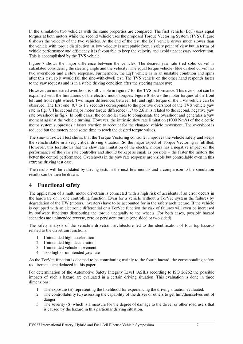
EVS27 International Battery, Hybrid and Fuel Cell Electric Vehicle Symposium 7
In the simulation two vehicles with the same properties are compared. The first vehicle (EqT) uses equal
torques at both motors while the second vehicle uses the proposed Torque Vectoring System (TVS). Figure
6 shows the velocity of the two vehicles. At the end of the test, the EqT vehicle drives much slower than
the vehicle with torque distribution. A low velocity is acceptable from a safety point of view but in terms of
vehicle performance and efficiency it is favourable to keep the velocity and avoid unnecessary acceleration.
This is accomplished by the TVS vehicle.
Figure 7 shows the major difference between the vehicles. The desired yaw rate (red solid curve) is
calculated considering the steering angle and the velocity. The equal torque vehicle (blue dashed curve) has
two overshoots and a slow response. Furthermore, the EqT vehicle is in an unstable condition and spins
after this test, so it would fail the sine-with-dwell test. The TVS vehicle on the other hand responds faster
to the yaw requests and is in a stable driving condition after the steering manoeuvre.
However, an undesired overshoot is still visible in figure 7 for the TVS performance. This overshoot can be
explained with the limitations of the electric motor torques. Figure 8 shows the motor torques at the front
left and front right wheel. Two major differences between left and right torque of the TVS vehicle can be
observed. The first one (0.7 to 1.7 seconds) corresponds to the positive overshoot of the TVS vehicle yaw
rate in fig. 7. The second major motor torque difference (1.7 to 2.6 s) is related to the second, negative yaw
rate overshoot in fig.7. In both cases, the controller tries to compensate the overshoot and generates a yaw
moment against the vehicle turning. However, the intrinsic slew rate limitation (1000 Nm/s) of the electric
motor system suppresses a faster reaction to account for the changed vehicle movement. The overshoot is
reduced but the motors need some time to reach the desired torque values.
The sine-with-dwell test shows that the Torque Vectoring controller improves the vehicle safety and keeps
the vehicle stable in a very critical driving situation. So the major aspect of Torque Vectoring is fulfilled.
However, this test shows that the slew rate limitation of the electric motors has a negative impact on the
performance of the yaw rate controller and should be kept as small as possible – the faster the motors the
better the control performance. Overshoots in the yaw rate response are visible but controllable even in this
extreme driving test case.
The results will be validated by driving tests in the next few months and a comparison to the simulation
results can be then be drawn.
4 Functional safety
The application of a multi motor drivetrain is connected with a high risk of accidents if an error occurs in
the hardware or in one controlling function. Even for a vehicle without a TorVec system the failures by
degradation of the HW (motors, inverters) have to be accounted for in the safety architecture. If the vehicle
is equipped with an electronic differential or a TorVec function the risk of failures will even be increased
by software functions distributing the torque unequally to the wheels. For both cases, possible hazard
scenarios are unintended reverse, zero or persistent torque (one sided or two sided).
The safety analysis of the vehicle’s drivetrain architecture led to the identification of four top hazards
related to the drivetrain functions:
1. Unintended high acceleration
2. Unintended high deceleration
3. Unintended vehicle movement
4. Too high or unintended yaw rate
As the TorVec function is deemed to be contributing mainly to the fourth hazard, the corresponding safety
requirements are deduced in this paper.
For determination of the Automotive Safety Integrity Level (ASIL) according to ISO 26262 the possible
impacts of such a hazard are evaluated in a certain driving situation. This evaluation is done in three
dimensions:
1. The exposure (E) representing the likelihood for experiencing the driving situation evaluated.
2. The controllability (C) assessing the capability of the driver or others to get him/themselves out of
danger.
3. The severity (S) which is a measure for the degree of damage to the driver or other road users that
is caused by the hazard in this particular driving situation.

EVS27 International Battery, Hybrid and Fuel Cell Electric Vehicle Symposium 8
Here we consider a drive on a country road with the typical speed of ~90 km/h. This is a very common
scenario occurring very frequently for the average driver. Therefore the highest rating E = 4 is assigned. In
this scenario an unintended yaw rate can lead to vehicle skidding and/or going off the lane. Most of the
drivers will not be able to master such a situation by keeping track with counter steering. Hence the highest
rating for the controllability C = 3 is chosen. By spontaneously applying an erroneous yaw rate it is very
likely that the vehicle will leave the road or hit other cars of the opposing traffic. Considering the high
speed of around 90 km/h life-threatening or fatal injuries have to be considered as very likely. This leads to
the highest rating for the severity S = 3. Following the rating scheme given in ISO 26262, these ratings lead
to an ASIL D overall rating for this hazard. This is the highest rating as per ISO 26262. The resulting safety
goal derived from this top hazard is: “Avoid too high or unintended yaw rate!” (SG4). The safe state for
this safety goal has been defined to “no torque application” because then the driver can keep control of the
vehicle by steering and braking. For failures with a lower severity or a better controllability the system will
turn in a degraded mode where both motors will receive equal torque requests (deactivation of TorVec). In
the degraded mode, the vehicle has a limited driving capability but the driver can continue his trip.
The safety concept for the safety goal 4 has been derived using the results of a fault tree analysis. Safety
requirements have been defined accordingly and attributed to the single vehicle functions. Here, the lean
and modular architecture was beneficial for the decomposition of the requirements to the functions since
the software blocks are small and well defined and the signal routes are simple, straight and non-branched.
The function chain contributing to the safety goal 4 (“Avoid too high or unintended yaw rate!”) is shown in figure 9. The ADAS functions do not contribute here as they cover only longitudinal functions. The
architecture allows for a clean separation between the different functional blocks. This makes it possible to
derive the safety concepts for these blocks rather independently. The safety concept for the vehicle status
acquisition in the Vehicle Observer relies on the model-based plausibility check of the observed values
from the sensors (steering angle, wheel speeds, yaw rate), thus leading to lower safety requirements for the
sensors. The TorVec function comprises several safety checks including
Compare actual yaw rate with driver request and counteract in case of discrepancies (for SG4).
Compare left and right torque request with overall acceleration request and limit torque request in
case of discrepancies.
Forward torque request if and only if the requests from the Decision Unit 1 are valid.
Finally, in the decision unit 2 (DU2) the proper application of the requested torques by the inverters /
motors is monitored and the safe state is enforced if critical failures occur.
Figure 9: Functions contributing to the requirements of safety goal 4.
All safety requirements have been included in the functions code and proven for effectiveness in various
tests. The same implementation strategy holds for the other safety goals, thus leading to a safe system
following the ISO 26262 requirements.
5 Conclusion
The implementation and performance of a Torque Vectoring function to and in a two front motor electric
drivetrain concept has been demonstrated. The TorVec function is part of a lean and scalable functional
architecture applicable to any kind of vehicle architecture by clear separation of core functions and
hardware interfaces and also allowing for an elegant consideration of functional safety. The safety
requirements for avoiding an unintended yaw rate have been explained for the functional chain including
EVS27 International Battery, Hybrid and Fuel Cell Electric Vehicle Symposium 9
TorVec. The TorVec algorithm follows an LPV control approach with encouraging results of good vehicle
stability for a sine-with-dwell test case. For fast controller performance the dynamics of the inverter-motor
system must be optimised. The validation and parameter adjustment will be performed in forthcoming
vehicle tests and will be presented in the conference talk.
References
[1] V. Scheuch, G. Kaiser, F. Holzmann, S. Glaser: Simplified architecture by the use of decision units; in:
Gereon Meyer (ed.): Advanced Microsystems for Automotive Applications 2012, Berlin, p. 121-130
[2] V. Scheuch, G. Kaiser, R. Straschill, F. Holzmann: A New Functional Architecture for the Improvement of
eCar Efficiency and Safety; 21st Aachen Colloquium Automobile and Engine Technology 2012, p. 1567-
1576
[3] www.efuture-eu.org
[4] M. Korte, F. Holzmann, V. Scheuch, and H. Roth: Development of an adaptive vehicle observer for an
electric vehicle; 2011 European Electric Vehicle Congress, Brussels
[5] Reza N. Jazar: Vehicle Dynamics: Theory and Applications; in: Springer 2009
[6] L. Chu, M. Xu, Y. Zhang, Y. Ou, Y. Shi: Vehicle Dynamics Based on Optimal Sliding Mode Control
Theory; in: International Conference on Computer, Mechatronics, Control and Electronic Engineering,
2010, p. 486 – 491
[7] M. Milehins, C. Cheng, T. Chu, R. Jones: Handling Behaviour of a TTR Hybrid Electric Vehicle with
Independent Rear Wheel Torque Control; in: International Symposium on Advanced Vehicle Control 2010,
p. 556 – 561
[8] J. Mohammadpour, C.W. Scherer: Control of Linear Parameter Varying Systems with Applications;
Springer, 2012
[9] G. Kaiser, Q. Liu, C. Hoffmann, M. Korte, H. Werner: Torque vectoring for an electric vehicle using an
LPV drive controller and a torque and slip limiter; Decision and Control (CDC), 2012 IEEE 51st Annual
Conference on , vol., no., pp.5016,5021, 10-13 Dec. 2012
[10] S. Tarbouriech, M. Turner: Anti-windup design: an overview of some recent advances and open problems;
in: IET Control Theory Appl., 2009, Vol. 3, No. 1, pp. 1–19
[11] C. Poussot-Vassal: Dissertation about “Commande Robuste LPV Multivariable de Châssis Automobile”; in: Grenoble Institut Polytechnique 2008
[12] H. Pacejka: Tyre and Vehicle Dynamics – Seccond Edition; in Elsevier 2006
[13] G. Forkenbrock, D. Elsasser, B. O’Harra: NHTSA’S Light Vehicle Handling and ESC Effectiveness Research Program, 2005
Authors
Volker Scheuch
Project leader for electro mobility at Intedis in Würzburg
Gerd Kaiser
PhD student at Intedis in Würzburg

EVS27 International Battery, Hybrid and Fuel Cell Electric Vehicle Symposium 10
Matthias Korte
PhD student at Intedis in Würzburg
Peter Grabs
Functional Safety Manager at Intedis in Würzburg
Fabian Kreft
System engineer at Intedis in Würzburg
Frédéric Holzmann
Manager of the Functional Architecture team at Intedis in Würzburg