d.4.5 wave setup, runup, and overtopping in the nearshore including wave setup, runup, and...

Guidelines and Specifications for Flood Hazard Mapping Partners [January 2005]

D.4.5-1 Section D.4.5

D.4.5 Wave Setup, Runup, and Overtopping

This section provides methodology for establishing the static and fluctuating water-level characteristics in the nearshore including wave setup, runup, and overtopping of sandy beaches and natural or constructed barriers. Additionally, procedures for calculating attenuation of waves propagating over flooded areas, including dissipative bottoms and through vegetation, are presented. D.4.5.1 Wave Setup and Runup

D.4.5.1.1 Introduction

The wave, meteorological, and bathymetric characteristics for the Pacific Coast are quite different from those on the Atlantic and Gulf coasts for which methodology to quantify the 1% chance water levels has been developed previously. The wave differences are due to the longer period waves and generally distant generation locations for the Pacific Coast whereas the meteorological differences are fewer hurricanes and thus lower winds. The major bathymetric differences are due to the relatively narrow Pacific Coast continental shelf widths. There are two major consequences of these differences for the 1% annual chance Pacific Coast hazards: (1) the wind surge component is relatively small due to the lower wind velocities coupled with the narrow shelf widths, and (2) the narrow spectra result in a substantial oscillating component of the wave setup with periods of tens to hundreds of seconds. Thus, the oscillating wave setup is a significant component of the total wave runup and a major contributor to coastal hazards on the Pacific Coast.

Wave setup and runup recommendations presented are based on a literature review, new developments, and comparison of available methods for quantifying these processes. Where possible, the most physics-based approaches have been identified and recommended.

D.4.5.1.2 Background, Definitions, and Approaches

Wave setup and runup contribute significantly to the damage potential of severe waves along the Pacific Coast. The total runup, R , includes three components: (1) static wave setup, η , (2)

dynamic wave setup, $η , and (3) incident wave runup, incR , i.e., conceptually:

$incR Rη η= + + (D.4.5-1)

in which η and $η are the magnitudes of the mean and oscillating wave setup components and Rinc the runup component due to the incident waves. In application, the two oscillating components ( $η and Rinc) are combined statistically to determine exceedance levels. Unless stated differently in this document, R refers to 2% runup conditions. The oscillating component of wave setup is a type of infragravity wave and is referred to here as dynamic wave setup. Each of the three components of total runup is defined and discussed below.

All policy and standards in this document have been superseded by the FEMA Policy for Flood Risk Analysis and Mapping. However, the document contains useful guidance to support implementation of the new standards.



Wave setup is the additional elevation of the water level due to the effects of transferring wave-related momentum to the surf zone. Momentum is transferred from winds to waves in the wave-generating area (usually in deep water for the Pacific Coast) and then is conveyed to shore by the waves similar to the manner that waves transport energy from the generating area to shore; see Figure D.4.5-1. A main difference between energy and momentum is that energy is dissipated in the surf zone whereas momentum is transferred to the water column. This transfer is equivalent to a shoreward-directed “push” on the water column that causes a tilt of the water surface; see Figure D.4.5-2. The wave setup is small and negative seaward of the surf zone (setdown) and begins to rise in the surf zone due to the transfer of momentum; see Figure D.4.5-3. If only one wave of a constant height and period were present, the wave setup would be steady.

Figure D.4.5-1. Schematic of Energy and Momentum Transfer from Winds to Waves within the Wave-generating Area, and to the Surf Zone and Related Processes




Figure D.4.5-2. Wave Setup Due to Transfer of Momentum

Figure D.4.5-3. Static Wave Setup Definitions at Still Water Level, oη ,

and Maximum Setup, maxη

For a single wave component, the static setup, η (h), at any water depth, h, can be expressed as:

2

2 2

(3 / 8) (3 / 8)( ) ( )16 1 (3 / 8) 1 (3 / 8)bh H hκ κ κη

κ κ= − + −

+ + (D.4.5-2)

where κ is the ratio (assumed a constant) of the breaking wave height to water depth within the surf zone and h is the still water depth, i.e., the depth in the absence of waves or wave effects. The wave setup at the still water line, oη , and the maximum wave setup, maxη , can be expressed from Equation D.4.5-2 in terms of the breaking wave height, bH :

Wind Direction

Wind Direction




2

(3 / 8)( )16 1 (3 / 8)o bHκ κη

κ= − +

+ (D.4.5-3)

The equivalent expression for the maximum wave setup, maxη , is:

2

max 2

2

(3 / 8)( )16 1 (3/ 8)

(3 / 8)(1 )1 (3 / 8)

bH

κ κκη

κκ

⎧ ⎫− +⎪ ⎪+⎪ ⎪= ⎨ ⎬

⎪ ⎪−⎪ ⎪+⎩ ⎭

(D.4.5-4)

For the usual value of κ = 0.78, the following relations result:

( ) 0.189 0.186bh H hη = − (D.4.5-5)

0.189o bHη = (D.4.5-6)

max 0.232 bHη = (D.4.5-7)

More realistic wave-breaking models that account for the actual profile will usually reduce the wave setup for the relatively mild profile slopes of the Pacific Coast. For a wave system consisting of more than one wave component (i.e., a wave spectrum), the breaking wave height in the above expressions is replaced by the root mean square breaking wave height, ( )b rms

H . Of significance on the Pacific Coast is that for wave systems consisting of more than one wave component, the setup is oscillating consisting of a steady and a so-called dynamic component; see Figure D.4.5-4. The dynamic wave setup component is larger for narrower wave spectra and is substantial on the Pacific Coast during extreme storms and thus will require quantification for

Figure D.4.5-4. Definitions of Static and Dynamic Wave Setup

and Incident Wave Runup




flood mapping purposes. In addition to contributing to the total wave runup and thus the shoreward reach of the waves, dynamic wave setup can carry floating debris such as logs at high velocities and thus increase the hazards and damage potential in coastal areas. Figure D.4.5-4 illustrates the three components that define the upper limit of wave effects.

Incident wave runup on natural beaches or barriers is usually expressed in a form originally due to Hunt (1959) in terms of the so-called Iribarren number, ξ , as follows:

mH L

ξ = (D.4.5-8)

in which m is a representative profile slope and is defined, depending on the application, as the beach slope or the slope of a barrier that could be either a dune or constructed element such as a breakwater or revetment. H and L are wave height and length, respectively. The wave characteristics in the Iribarren number can be expressed in terms of breaking or deep water characteristics. For purposes here, two wave characteristics in the Iribarren number are used including that based on the significant deep water wave height, oH , and peak or other wave period, T, of the deep water spectrum, and that based on the significant wave height at the toe of a barrier. The first definition for a sandy beach is as follows:

o

o o

mH L

ξ = (D.4.5-9)

where Lo is the deep water wave length:

2

2ogL Tπ

= (D.4.5-10)

and g is the gravitational constant. The beach profile slope is the average slope out to the breaking depth associated with the significant wave height. Other definitions of the Iribarren number are defined later in this section as needed.

The 2% incident wave runup on natural beaches, incR , is expressed in terms of the Iribarren number as:

0.6inc oo o

mR HH L

= (D.4.5-11)

Several definitions are relevant to the determination of runup and overtopping considered later in this section. The term still water level (SWL) has an accepted definition in coastal engineering as the water level in the absence of wind waves and their effects and thus would include the astronomical tide, El Niño, and surge due to wind effects, but would not include either of the wave setup components. However, the wave setup components are included in the base water level for calculating wave runup and overtopping. Thus, the term static water level (STWL) is




defined here as the sum of the SWL and the static wave setup, η . Terminology is also useful to describe the sum of the static water level and a X% dynamic wave setup component. For purposes here, this will be defined as the dynamic water level X% (DWLX%). For example, the elevation corresponding to a 2% Dynamic Water Level would be the sum of the SWL (including astronomical tide, El Niño, and wind surge if present), the static wave setup, and the 2% dynamic wave setup. The term reference water level (RWL) is used as general terminology to refer to the water level that is appropriate for the particular application being discussed. As defined in Section D.4.2, the total water level (TWL) is the sum of the SWL, the wave setup, and wave runup.

D.4.5.1.3 General Input Requirements

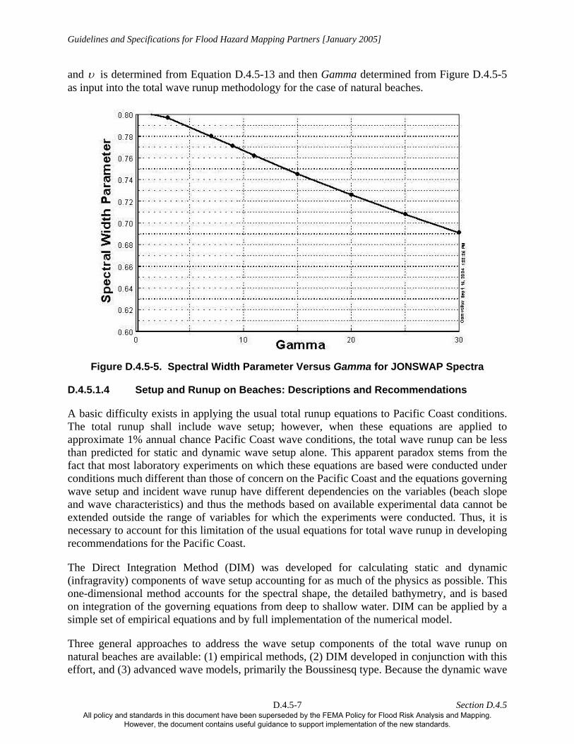
The wave transformation element of the Guidelines and Specifications (Section D.4.4) produces a nearshore shallow water wave spectrum outside the breaking zone and an equivalent deep water wave spectrum. The approaches detailed in the following subsections base the total wave runup on the equivalent deep water wave spectrum for the case of natural beaches or for the case of runup on a barrier, the significant wave height at the toe of the barrier. To apply some of these methods, a parameterized (Joint North Sea Wave Project [JONSWAP]) spectrum is developed. The following wave characteristics are quantified: (1) equivalent deep water significant wave height, (2) peak wave period, and (3) spectral width (here spelled out as Gamma to avoid confusion with the Greek letter γ used to denote other parameters in this subsection). Large values of Gamma are associated with narrow spectra. Additionally, in some of the methods, an approximate uniform nearshore slope of the profile, m, must be established.

The deep water significant wave height and the peak period can be determined using the information provided from the wave transformation output. The recommended basis for determination of the spectral peakedness parameter (Gamma) is described below.

A parameter defined by Longuet-Higgins to quantify the spectrum narrowness (or peakedness) is based on the moments of the frequency spectrum, mi, defined previously as Equation D.4.4-21 in Section D.4.4 and refined below as Equation D.4.5-12:

1

( )N

ii n n

nm f S f

=

=∑ (D.4.5-12)

where S(fn) is the wave energy at the discrete frequency, fn . The Longuet-Higgins definition of the spectral narrowness, υ , is expressed in terms of the spectral moments:

1/ 2

221

1om mm

υ⎡ ⎤

= −⎢ ⎥⎣ ⎦ (D.4.5-13)

such that for an infinitely narrow spectrum, υ = 0. For purposes here, the two spectral peakedness parameters, υ and Gamma, have been plotted for JONSWAP spectra and the results are presented in Figure D.4.5-5. The spectral moments, m0, m1, and m2, for the actual equivalent deep water spectrum are provided from the wave transformation analysis effort (Section D.4.4),




and υ is determined from Equation D.4.5-13 and then Gamma determined from Figure D.4.5-5 as input into the total wave runup methodology for the case of natural beaches.

Figure D.4.5-5. Spectral Width Parameter Versus Gamma for JONSWAP Spectra

D.4.5.1.4 Setup and Runup on Beaches: Descriptions and Recommendations

A basic difficulty exists in applying the usual total runup equations to Pacific Coast conditions. The total runup shall include wave setup; however, when these equations are applied to approximate 1% annual chance Pacific Coast wave conditions, the total wave runup can be less than predicted for static and dynamic wave setup alone. This apparent paradox stems from the fact that most laboratory experiments on which these equations are based were conducted under conditions much different than those of concern on the Pacific Coast and the equations governing wave setup and incident wave runup have different dependencies on the variables (beach slope and wave characteristics) and thus the methods based on available experimental data cannot be extended outside the range of variables for which the experiments were conducted. Thus, it is necessary to account for this limitation of the usual equations for total wave runup in developing recommendations for the Pacific Coast.

The Direct Integration Method (DIM) was developed for calculating static and dynamic (infragravity) components of wave setup accounting for as much of the physics as possible. This one-dimensional method accounts for the spectral shape, the detailed bathymetry, and is based on integration of the governing equations from deep to shallow water. DIM can be applied by a simple set of empirical equations and by full implementation of the numerical model.

Three general approaches to address the wave setup components of the total wave runup on natural beaches are available: (1) empirical methods, (2) DIM developed in conjunction with this effort, and (3) advanced wave models, primarily the Boussinesq type. Because the dynamic wave




setup is considered to be very significant on Pacific Coast shorelines and depends on the spectral width and DIM is the only method (other than the Boussinesq models) that can account for variable spectral width, DIM is the preferred method for application.

D.4.5.1.4.1 Direct Integration Method

Because the DIM approach does not include the effects of incident wave runup, it is recommended that the 2% incident runup be incorporated and added statistically as discussed in more detail later. The recommended formulation is:

inc R o oR F Hξ= (D.4.5-14)

The coefficient RF in the above equation will differ for sandy beaches and barriers as discussed in the following subsections. The DIM approach allows the wave and bathymetric characteristics to be taken into consideration. Specifically, the spectral shape and actual bathymetry can be represented. A detailed discussion of the DIM program is presented in a User’s Manual in the supporting documentation to these Guidelines and Specifications. Two applications of DIM are available to the Mapping Partner: the computer program and a set of equations. The equations available are based on parameterized spectra (the JONSWAP spectrum that allows various spectral widths to be considered) and uniform profile slopes. The program DIM calculates the total wave setup and provides as output the static (average) wave setup, η , and the root mean square (rms), rmsη , of the fluctuating wave setup around the average. Static and dynamic wave setup increase with wave period and the rms of the fluctuating setup component has been found to increase with the narrower spectra. The static setup component, η , and rms of the dynamic setup component, rmsη , can be determined using the DIM program or the following equations:

4.0 H T Gamma SlopeF F F Fη = (D.4.5-15)

and

2.7rms H T Gamma SlopeG G G Gη = (D.4.5-16)

where the units of η and rmsη are in feet and the factors are for wave height (FH and GH), wave period , (FT and GT), JONSWAP spectrum narrowness factor (FGamma and GGamma), and nearshore slope (FSlope and GSlope). These factors are defined in Table D.4.5-1. With the exception of the spectral narrowness factors, the F and G factors are the same. The nearshore slope is the average slope between the runup limit and twice the break point of the significant wave height with the depth, bh , at this point defined as hb = Hb / κ . For purposes here, κ can be taken as 0.78. Because the wave setup components vary with the 0.2 power of this effective slope, these values are not overly sensitive to the value of effective slope.




In applying the DIM method (whether from the program DIM or from the equations and Table D.4.5-1), it is necessary to develop the statistics of the oscillating wave setup and incident wave runup. This combination is based on the rms values (or standard deviations, σ ) of each component. The standard deviation of setup fluctuations, 1( )rmsσ η≡ , is determined from the program or from the guidance provided in Table D.4.5-1. The recommended standard deviation for the incident wave oscillations, 2σ , on natural beaches is given by:

2 0.3 o oHσ ξ= (D.4.5-17)

and the standard deviation associated with the relatively steep barriers is addressed later. With the two standard deviations ( 1σ and 2σ ) available, the total oscillating contribution to the 2%

total wave runup, $Tη , is determined as the combination of the two standard deviations of the fluctuating components, 1 2andσ σ :

$ 2 21 22.0Tη σ σ= + (D.4.5-18)

The results of the computations using DIM suggest that the fluctuating component of the wave setup is normally distributed and that the maxima of the fluctuating component of wave setup are Rayleigh-distributed, similar to the general behavior found by Hedges and Mase (2004) in laboratory experiments of wave setup and wave runup.

D.4.5.1.4.2 Advanced Wave Models

Wave models are becoming more sophisticated and able to account for the complexities of water waves. A rapidly developing class of these is the so-called Boussinesq models, which are both commercially and publicly available with the commercial models generally being the more user friendly. In addition to wave setup, Boussinesq models can calculate wave runup. In conjunction with the development of these Guidelines and Specifications, one-dimensional Boussinesq models have been applied to calculate total wave runup and the average and oscillating components were calculated separately. The comments below are based on an assessment of these Boussinesq results.

Based on comparison with other methods, Boussinesq models yield generally realistic results. The main concern with Boussinesq modeling is the “learning curve” required to carry out these types of computations with confidence. Additionally, it was difficult to carry out calculations for

Table D.4.5-1. Summary of Factors to Be Applied with DIM

Factor for

Variable Wave Height Wave Period Spectral

Narrowness Nearshore Profile

Slope η ( )0.826.2oH ( )0.420.0T 1.0 ( )0.20.01m

rmsη ( )0.826.2oH ( )0.420.0T ( )0.16Gamma ( )0.20.01m




deep water waves with a small directional dependency. The reason for this difficulty lies in the associated substantial longshore wave lengths and the need for them to be represented by a two-dimensional model. One possible Federal Emergency Management Agency (FEMA) application that would avoid the repeated learning curve requirement would be to carry out computations on a regional basis using Boussinesq models. The rate of improvement/development of Boussinesq models is moderate at present; however, it is likely that this type of model will be much more capable in 10 to 20 years than at present. Thus, at this stage, a Mapping Partner may elect to apply Boussinesq models; however, for application on a regional basis, it is preferable to wait for further developments and improvements. If a Boussinesq model is applied, the Mapping Partner shall obtain FEMA approval and it is suggested that calculations also be carried out using the DIM methodology for comparison of results.

D.4.5.1.5 Runup on Barriers

D.4.5.1.5.1 Special Considerations Due to Dynamic Wave Setup

Previous discussions have emphasized that a large wave runup event on the Pacific Coast is anticipated to have a more substantial dynamic wave setup than is present in the database on which available runup methods are based. Thus, special consideration is required in the calculation of wave runup and wave overtopping, which is the subject of a later subsection. The issues are to include the dynamic wave setup appropriately without double inclusion of the static and dynamic wave setup components that are inherent in the empirical database from which the runup and overtopping methodology were based. Table D.4.5-2 describes the recommended methodology for both open coast and sheltered water settings. This methodology is illustrated through example calculations and separate supporting documentation.

Table D.4.5-2. Recommended Procedure to Avoid Double Inclusion of Wave Setup Components

Case Procedure Open Coast, Sandy Beach Apply DIM for wave setup with statistically combined incident

runup, Equations D.4.5-17 and D.4.5-18 Open Coast, Coastal Barrier Present Apply DIM for wave setup and reduce dynamic wave setup by

amount considered to be most likely present in laboratory tests on which runup equations are based

Sheltered Waters, Sandy Beach Same as open coast, sandy beach Sheltered Waters, Coastal Barrier Present

Same as open coast, coastal barrier present

D.4.5.1.5.2 Methodology for Calculating Wave Runup on Barriers

In this subsection, barriers include steep dune features and coastal armoring structures such as revetments. Runup elevations on barriers depend not only on the height and steepness of the incident wave (and its interaction with the preceding wave), but also on the geometry (and construction) of the structure. Runup on structures can also be affected by antecedent conditions resulting from the previous waves and structure composition. Due to these complexities, runup on structures is best calculated using equations developed with tests on similar structures with




similar wave characteristics. Runup equations generally take the form of Equation D.4.5-14, with coefficients developed from laboratory or field experiments. Following Equation D.4.5-1, the incident wave runup (Rinc) for structures is added to the wave setup values (η and $η ) statistically based on application of DIM. Also, DIM is applied to estimate the setup water surface at the toe of the structure, as appropriate, in most cases where the structure toe will be within the surf zone.

The recommended approach to calculating wave runup on structures is based on the Iribarren number (ξ) and reduction factors developed by Battjes (1974), van der Meer (1988), de Waal & van der Meer (1992), and described in the Coastal Engineering Manual (CEM) (USACE, 2003). The approach is referred to as the TAW (Technical Advisory Committee for Water Retaining Structures) method and is clearly articulated in van der Meer (2002) and includes reduction factors for surface roughness, the influence of a berm, structure porosity, and oblique wave incidence. The TAW method is useful as it covers a wide range of wave conditions for calculating wave runup on both smooth and rough slopes. In addition to being well documented, the TAW method agrees well with both small- and large-scale experiments.

It is important to note that other runup methods and equations for structures of similar form may provide more accurate results for a particular structure. The Mapping Partner shall carefully evaluate the applicability of any runup method to verify its appropriateness. Figure D.4.5-6 shows a general cross-section of a coastal structure, a conceptual diagram of wave runup on a structure, and definitions of parameters.

Figure D.4.5-6. Runup on Coastal Structures, Definition Sketch

Most of the wave runup research and literature shows a clear relationship between the vertical runup elevation and the Iribarren number. Figure D.4.5-7 shows the relative runup (R/Hmo) plotted against the Iribarren number for two different methods: (1) van der Meer (2002), and (2) Hedges & Mase (2004). In Figure D.4.5-7, both runup equations are derived from laboratory experimental data and are plotted within their respective domains of applicability for the Iribarren number. Each equation shows a consistent linear relationship between the relative

SWL + $η η+ = DWL2% Total Runup

Still Water Level (SWL)

Total Water Level

Armor Layer




runup and ξom for values of ξom below approximately 2. For values of ξom above approximately 2, only the van der Meer method is applicable. Moreover, due to its long period of availability and wide international acceptance, the van der Meer relationship (also referred to as the TAW runup methodology) is recommended here. The Mapping Partner shall characterize the wave conditions in terms of ξom and be aware of the runup predictions provided by the various methods available in the general literature.

0 1 2 3 40

1

2

3

Iribarren Number, ξom

Non

Dim

ensi

onal

Tot

al R

unup

, R/H

mo

Hedge

s and

Mas

e (20

04)

TAW (van der Meer, 2002)

Figure D.4.5-7. Non-dimensional Total Runup vs. Iribarren Number

The general form of the wave runup equation recommended for use is (modified from van der Meer, 2002):

1.77 0.5 1.8

1.64.3 1.8

r b P om b om

mor b P b om

om

R Hβ

β

γ γ γ γ ξ γ ξ

γ γ γ γ γ ξξ

≤ <⎧ ⎫⎪ ⎪⎪ ⎪⎛ ⎞= ⎨ ⎬

− ≤⎜ ⎟⎪ ⎪⎜ ⎟⎪ ⎪⎝ ⎠⎩ ⎭

(D.4.5-19)

where:

R is the 2% runup = 2 2σ

moH = spectral significant wave height at the structure toe

rγ = reduction factor for influence of surface roughness

bγ = reduction factor for influence of berm γβ = reduction factor for influence of angled wave attack γP = reduction factor for influence of structure permeability




Equations for quantifying the γ parameters are presented in Table D.4.5-3. The reference water level at the toe of the barrier for runup calculations is DWL2%. Additionally, because some wave setup influence is present in the laboratory tests that led to Equation D.4.5-19, the following adjustments are made to the calculation procedure for cases of runup on barriers.

Table D.4.5-3. Summary of γ Runup Reduction Factors

Runup Reduction Factor Characteristic/Condition Value of γ for Runup

Smooth Concrete, Asphalt and Smooth Block

Revetment

rγ = 1.0

1 Layer of Rock With Diameter, D.

/sH D = 1 to 3.

rγ = 0.55 to 0.60

2 or More Layers of Rock. /sH D = 1.5 to 6.

rγ = 0.5 to 0.55

Roughness Reduction Factor,

rγ

Quadratic Blocks rγ = 0.70 to 0.95. See Table V-5-3

in CEM for greater detail

(D.4.5-20)

Berm Section in Breakwater,

bγ , B = Berm Width,

hdx

π⎛ ⎞⎜ ⎟⎝ ⎠

in radians

Berm Present in Structure Cross-section. See Figure D.4.5-8 for Definitions of

B, Lberm, and Other Parameters

1 1 cos , 0.6 1.02

hb B

berm

dBL x

πγ γ⎡ ⎤⎛ ⎞= − + < <⎜ ⎟⎢ ⎥⎝ ⎠⎣ ⎦

0

2 0 2

h

mo mo

hmo

mo

dRR ifH H

xdH if

H

−⎧ ≤ ≤⎪⎪= ⎨⎪ ≤ ≤⎪⎩

(D.4.5-21)

Minimum and maximum values of bγ = 0.6 and 1.0, respectively

Long-Crested Waves βγ

1.0, 0 10

cos( 10 ),10 63

0.63, 63

o

o o o

o

β

β β

β

⎧ < <⎪⎪= − < <⎨⎪ >⎪⎩

(D.4.5-22)

Wave Direction Factor, βγ ,

β is in degrees and = 0o for normally incident waves

Short-Crested Waves 1 0.0022 , 80

1 0.0022 80 , 80

o

o

β β

β

− ≤

− ≥ (D.4.5-23)

Porosity Factor, Pγ

Permeable Structure Core Pγ = 1.0, omξ < 3.3; Pγ = 0.46

2.01.17( )omξ

, omξ > 3.3

and porosity = 0.5. for smaller porosities, proportion Pγ according to porosity . See Figure D.4.5-9 for definition of porosity

(D.4.5-24)




Figure D.4.5-8. Berm Parameters for Wave Runup Calculations

Figure D.4.5-9. Structure Porosity Definition

The steps below are based on the consideration of laboratory tests conducted with a JONSWAP Gamma equal to 3.3, which is the average of the spectra entering into the development of the JONSWAP spectrum. Also, see Table D.4.5-2.

1. Calculate, using DIM methodology, $ rmsη (= 1σ ) for: (1) Gamma equal to 3.3, and (2) the Gamma value of interest for the 1% percent chance conditions.

2. Reduce the dynamic wave setup at the toe of the structure by the difference between the 2% dynamic wave setup values associated with the Gamma of interest and Gamma = 3.3, i.e., 1σ (Gamma > 3.3) = 1σ (Gamma of interest) - 1σ (Gamma = 3.3). For cases in which the Gamma of interest is less than 3.3, set the value of 1σ = 0 (Equations D.4.5-17 and D.4.5-18).

dh

Lberm

Hmo

Hmo B




For a smooth impermeable structure of uniform slope with normally incident waves, each of the γ runup reduction factors is 1.0.

In calculating the Iribarren number to apply in Equation D.4.5-19, the Mapping Partner shall use Equation D.4.5-9 and replace Ho with Hmo and replace T with Tm-1.0 (the spectral wave period) in Equation D.4.5-10. Hmo and Tm-1.0 are calculated as:

omo mH 0.4= (D.4.5-25)

1.10.1p

m

TT =− (D.4.5-26)

where Hmo is the spectral significant wave height at the toe of the structure and Tp is the peak wave period. In deep water, Hmo is approximately the same as Hs, but in shallow water, Hmo is 10-15% smaller than the Hs obtained by zero up crossings (van der Meer, 2002). In many cases, waves are depth-limited at the toe of the structure and Hb can be substituted for Hmo, with Hb calculated using a breaker index of 0.78 unless the Mapping Partner can justify a different value. The breaker index can be calculated based on the bottom slope and wave steepness by several methods, as discussed in the CEM (USACE, 2003). As noted, the water depth at the toe of the structure shall include the static wave setup and the 2% dynamic wave setup, calculated with DIM. In terms of the Iribarren number, the TAW method is valid in the range of 0.5 < ξom < 8-10, and in terms of structure slope, the TAW method is valid between values of 1:8 to 1:1. The Iribarren number as described above is denoted omξ as indicated in Equation D.4.5-19.

Runup on structures is very dependent on the characteristics of the nearshore and structure geometries. Hence, better runup estimates may be possible with other runup equations for particular conditions. The Mapping Partner may use other runup methods based on an assessment that the selected equations are derived from data that better represent the actual profile geometry or wave conditions. See CEM (USACE, 2003) for a list of presently available methods and their ranges of applicability.

D.4.5.1.5.3 Special Cases—Runup from Smaller Waves

In some special cases, neither of the previously described methods (Subsection D.4.5.1.4, Setup and Runup Beaches: Description and Recommendations, or Subsection D.4.5.1.5 Runup on Barriers) is applicable. These special cases include steep slopes in the nearshore with large Iribarren numbers or conditions otherwise outside the range of data used to develop the total runup for natural beach methods. Also, use of the TAW method is questionable where the toe of a structure, or naturally steep profile such as a rocky bluff, is high relative to the water levels, limiting the local wave height and calculated runups to small values. In these cases, it is necessary to calculate runup with equations of the form of Equation D.4.5.1-19 and to avoid double inclusion of the setup as discussed in Subsections D.4.5.1.5.1 and D.4.5.1.5.2 and Table D.4.5-2 and to carry out the calculations at several locations across the surf zone using the average slope in the Iribarren number. With this approach, it is possible that calculations with the largest waves in a given sea condition may not produce the highest runup, but that the highest runup will be the result of waves breaking at an intermediate location within the breaking zone.




The recommended procedure is to consider a range of (smaller) wave heights inside the surf zone in runup calculations. For this approach, for all depths considered, the dynamic setup is reduced if the Gamma of interest exceeds 3.3 as described in Subsections D.4.5.1.5.1 and D.4.5.1.5.2 and Table D.4.5-2. For each depth considered, the static setup is calculated with Equation D.4.5-5 with the water level including the 2% dynamic wave setup replacing the depth, h, in that equation. With the 2% dynamic water level available, methods of calculating wave runup on barriers is applied and are described in greater detail below.

The concept of a range of calculated runup values is depicted schematically in Figure D.4.5-10 where an example transect and setup water surface profile are shown. Figure D.4.5-10 also shows the corresponding range of depth-limited breaking wave heights calculated based on a breaker index and plotted by breaker location on the shore transect. The Iribarren number was also calculated and plotted by breaker location in Figure D.4.5-10. The calculation of ξ at each location uses the deshoaled deepwater wave height corresponding to the breaker height, the deepwater wave length and the average slope calculated from the breaker point to the approximate runup limit. Note that this average slope (also called composite slope, as defined in the CEM [USACE, 2003] and SPM [USACE, 1984] increases with smaller waves because the breaker location approaches the steeper part of the transect near the shoreline. This increases the numerator in the ξ equation. Also, the wave height decreases with shallower depths, reducing the wave steepness in the denominator of the ξ equation. Hence, as plotted in Figure D.4.5-10, ξ increases as smaller waves closer to shore are examined, increasing the relative runup (R/H). However, because the wave height decreases, the runup value, R, reaches a maximum and then decreases.

The following specific steps are used to determine the highest wave runup caused by a range of wave heights in the surf zone:

1. Calculate, using DIM, the reduced 2% dynamic wave setup based on the Gamma of interest and Subsections D.4.5.1.5.1 and D.4.5.1.5.2 and Table D.4.5-2. Calculate the static wave setup based on Equation D.4.5-5 for the cross-shore location considered. Replace h in that equation with the sum of the still water depth at the location and the 2% dynamic wave setup.

2. Calculate the runup using the methods described earlier for runup on a barrier. This requires iteration for this location to determine the average slope based on the differences between the runup elevation and the profile elevation at the location and the associated cross-shore locations. Iterate until the runup converges for this location.

3. Repeat the runup calculations at different cross-shore locations until a maximum runup is determined.




Figure D.4.5-10. Example Plot Showing the Variation of Surf Zone Parameters

y

Breaker Location Causing Maximum Runup

Cross-shore Distance, y

Wave Runup at Shoreline Resulting From Breaking at Cross-shore Location, y

Depth Limited Wave Height

Var

iabl

es a

s a F

unct

ion

of B

reak

er L

ocat

ion

Iribarren Number

2% Setup Level

Total Maximum Potential Runup




D.4.5.1.6 Example Computations of Total Runup

Four examples corresponding to the four settings in Table D.4.5-2 are examined and total runup values presented. The conditions for the four examples are presented in Table D.4.5-4. These examples have been selected to illustrate application of the methodology for several settings. The supporting documents provide a detailed step-by-step presentation of the calculations associated with these four examples and seven additional examples..

Table D.4.5-4. Example Characteristics

Example Water Level and Wave Conditions

Profile Conditions Barrier Characteristics

1. Open Coast, Sandy Beach

Astronomical tide = 3 feet above NAVD* and wind surge = 2 feet. moH = 26.2 feet; T = 20 sec; Gamma = 30 in JONSWAP spectrum

Slope = 1:60 No barrier

2. Open Coast With Structure Present

Same as Example 1 Slope = 1:60 Slope = 1:1.5, 1 layer rock of 3 feet diameter, toe depth = 2 feet below NAVD. porosity considered to be 0.2

3. Sheltered Water, Sandy Beach

Astronomical tide = 3 feet, above NAVD and wind surge = 1 foot. moH = 6.0 feet; T = 5 sec; Gamma = 1 in JONSWAP spectrum

Slope = 1:60 No barrier

4. Sheltered Water With Structure Present

Same as Example 3 Slope = 1:60 Same as Example 2

* NAVD = North American Vertical Datum Example 1: Open Coast, Sandy Beach

The actual bathymetry for this example is presented in Figure D.4.5-11 and is approximated here as a uniformly sloping profile with slope of 1:60 out to twice the approximate significant wave height breaking point. The deep water Iribarren number, oξ , for this case is calculated to be 0.147.

Table D.4.5-5 presents the 2% exceedance results based on the DIM program and coefficients in Table D.4.5-1 with a nearshore slope of 1:60 as well as the results from the Boussinesq model calculations. To illustrate the role of the spectral width, the results for a Gamma of unity based on the equations have been presented as a footnote to Table D.4.5-5.




Figure D.4.5-11. Offshore Profile for Example Problem

Table D.4.5-5. Comparison of Results from Various Methods of

Calculating 2% Total Runup for Examples

2% Total Runup (ft)

Example Method

Static Setup

(ft)

Combined Dynamic Setup and Incident Wave Runup

(ft)

Total Runup

(ft) 1 Boussinesq Equations 5.33 8.71 14.041 DIM Program 4.89 10.11 15.53*

1 Equations (Table D.4.5-1)

Based on DIM 4.43 10.58 15.01

2 Equations (Table D.4.5-1) Based on DIM and Equation D.4.5-19 4.43 23.44 27.87

3 Equations (Table D.4.5-1)

(Based on DIM) 0.78 1.10 1.88

4 Equations (Table D.4.5-1) Based on DIM and Equation D.4.5-19 0.78

9.20 (Incident Wave Runup) (Dynamic Setup = 0.0) 9.98

* Note: For a Gamma (JONSWAP spectral peakedness) value of 1.0, the 2% total runup by the DIM method is 10.85 feet. The total runup for all examples is above SWL.




Example 2: Open Coast with Structure Present

The runup reduction factors determined for this example from Table D.4.5-3 are: rγ = 0.6, bγ = 1.0, βγ = 1.0, and Pγ = 0.86. Values of the runup were based on the DIM methodology and Equation D.4.5-19 with adjustment for the dynamic setup considered to occur in the model tests that led to Equation D.4.5-19. The total 2% dynamic water depth at the toe of the structure was found to be 14.49 feet, which yielded an approximate significant wave height at the structure toe of 11.30 feet for use in Equation D-4.5-19. The value of omξ is 8.16. The total runup above SWL was determined to be 27.87 feet.

Example 3: Sheltered Waters, Natural Beach

The deep water Iribarren number based on the conditions in this example is: oξ = 0.077. The total 2% runup above SWL was determined to be 1.88 feet.

Example 4: Sheltered Waters with Structure Present

The runup reduction factors determined for this example were obtained from Table D.4.5-3 and are the same as for Example 2: rγ = 0.6, bγ = 1.0, βγ = 1.0, and Pγ = 0.86. The total runup value was based on the DIM methodology and Equation D.4.5-19 with adjustment for the dynamic setup considered to occur in the model tests that led to Equation D.4.5-19. This resulted in a dynamic setup, rmsη = 0. The total 2% dynamic water depth at the toe of the structure was found to be 6.78 feet resulting in moH =5.29 feet. The relevant Iribarren number at the breakwater toe is: omξ = 2.95. The total runup elevation above SWL was determined to be 9.98 feet.

D.4.5.1.7 Documentation

The Mapping Partner shall document the procedures and values of parameters employed to establish the 1% chance total wave runup on the various transects on natural beaches and barriers that could include steep dunes and structures. In particular, the basis for establishing the runup reduction factors and their values shall be documented. The documentation shall be especially detailed in case the methodology deviates from that described herein and/or in the recommendations in the supporting documentation. Any measurements and/or observations shall be recorded as well as documented or anecdotal information regarding previous major storm- induced runup. Any notable difficulties encountered and the approaches to addressing them shall be described clearly.

D.4.5.2 Overtopping

D.4.5.2.1 Overview

Wave overtopping occurs when the barrier crest height is lower than the potential runup level; waves running up the face of a barrier reach and pass over the barrier crest. If the total runup elevation (calculated in Subsection D.4.5.1) exceeds the crest elevation, zc, then the overtopping of the structure is potentially significant and requires evaluation to define hazard zones.




There are three physical forms of overtopping:

1. Green water overtopping occurs when waves break onto or over the barrier and the overtopping volume is relatively continuous.

2. Splash overtopping occurs when waves break seaward of the face of the structure, or where the barrier is high in relation to the wave height, and overtopping is a stream of droplets. Splash overtopping can be carried over the barrier under its own momentum or may be driven by onshore wind.

3. Spray overtopping is generated by the action of wind on the wave crests immediately offshore of the barrier. Without the influence of a strong onshore wind, this spray does not contribute to significant overtopping volume.

Mapping hazard zones due to green water and splash overtopping requires an estimate of the velocity or discharge of the water that is propelled over the crest, and the envelope of the water surface, defined by the water depth, landward of the crest. Ideally:

● Base Flood Elevations (BFEs) are determined based on the water surface envelope landward of the barrier crest.

● Hazard zones are determined based on the inland extent of greenwater and splash overtopping, and on the depth and force of flow in any sheet flow areas.

The calculation methods for the hazard zones landward of the barrier crest differ for green water overtopping and splash overtopping and depend on the ratio '/ 'cR z as illustrated in Figure D.4.5-12. For 1 < '/ 'cR z < 2, splash overtopping dominates and for '/ 'cR z > 2, bore propagation dominates. Each of these types results in the occurrence of a hazard zone, although the calculations quantifying the hazard zones differ as described later in this subsection. Note that 'R and 'cz are relative to the DWL2%.

Figure D.4.5-13 shows the parameters that may be available for use in mapping BFEs and flood hazard zones and are listed in Table D.4.5-6 (availability depends on the runup and overtopping methods employed). Again, the reference water level for overtopping calculations is the DWL2%. The remainder of this subsection is organized as follows. First the methodology for calculating overtopping rates is reviewed. Secondly, methods are presented for calculating the hazard zones landward of the crest of the barrier for the two types of overtopping discussed above and illustrated in Figure D.4.5-12.




a) Conditions for Splash Overtopping

b) Conditions for Bore Propagation Overtopping

Figure D.4.5-12. Definition Sketch for Two Types of Overtopping

'cz

Bore

DWL2%

'R

'/ 'cR z > 2 Propagating Bore Occurs

Potential Runup

Splash Over

DWL2%

'R'cz

1 < '/ 'cR z < 2 Splash Over Occurs

Potential Runup




Figure D.4.5-13. Parameters Available for Mapping BFEs and Flood Hazard Zones

Table D.4.5-6. Overtopping Parameters Used in Hazard Zone Mapping

Parameter Variable UnitsTotal potential runup elevation R ft Mean overtopping rate q cfs/ft Landward extent of green water and splash overtopping yG,Outer ft Depth of overtopping water at a distance y landward of crest h(y) ft

Due to the complexity of overtopping processes and the wide variety of structures over which overtopping can occur, wave overtopping is highly empirical and generally based on laboratory experimental results and on relatively few field investigations.

D.4.5.2.2 Background

Overtopping calculations are subject to more uncertainty than runup calculations. While runup models may replicate observed runup values with errors of about 20%, predicted overtopping rates are often in error by a factor of 2 or more (Kobayashi, 1999). Some overtopping predictions may be even less accurate, given the fact that subtle changes in wave conditions, water level, structure geometry and characteristics can have a very large effect on overtopping rates.

D.4.5.2.2.1 Empirical Equations

Wave overtopping may be predicted by a number of different methods, but chiefly by semi- empirical equations that have been fitted to hydraulic model tests using irregular waves for specific structure geometries. These empirical equations have the general form:

( )'bFQ a e−

= or '( ) bQ a F −= (D.4.5-27)

y

z

R∆




where Q is a dimensionless average discharge per unit length of structure and F’ is a dimensionless freeboard. It is noted that these two dimensionless quantities are defined differently depending on the researcher and the structure characteristics. Overtopping rates predicted by these formulae generally include green water and splash overtopping because both parameters are recorded during the model tests.

Section VI-5-2b of the CEM (USACE, 2003) describes several different methods that have been developed for particular geometries. The choice of method depends upon the form of wave behavior at or on the structure, and the nature of the structure.

D.4.5.2.2.2 Types of Wave Behavior

Any discussion on wave-structure interaction requires that the key wave processes be categorized, so these different processes may be separated. Four key terms, non-breaking or breaking on normally sloped structures and reflecting or impacting on steeper structures, are defined below to describe breaking and overtopping processes.

For beaches and normally sloping structures, the simplest division is to separate breaking conditions where waves break on the structure from non-breaking waves. These conditions can be identified using the surf similarity parameter (or Iribarren number) defined in terms of beach or structure slope (tan α), and wave steepness (Hmo/Lo):

tan tanop

mo op

o

H SL

α αξ = = (D.4.5-28)

where opS is wave steepness as defined above.Breaking on normally sloped (1:1.5 to 1:20) surfaces generally occurs where ξop ≤ 1.8, and non-breaking conditions when ξop > 1.8.

On very steep slopes or vertical walls, reflecting overtopping occurs when waves are relatively small in relation to the local water depth and of lower wave steepness. The structure toe or approach slope does not critically influence these waves. Waves run up and down the wall, giving rise to relatively smoothly varying loads. In contrast, impacting breaking on steep slopes occurs when waves are larger in relation to local water depths, perhaps shoaling up over the approach bathymetry or structure toe itself.

For simple vertical walls, the division between reflecting and impacting conditions is made using the parameter *h .

* 2

2

mo m

h hhH gT

π⎛ ⎞= ⎜ ⎟

⎝ ⎠ (D.4.5-29)

Reflecting conditions can generally be said to occur where *h ≥ 0.3, and impacting conditions when *h < 0.3.




D.4.5.2.2.3 Nature of the Structure

The relative freeboard, Fc/Hs, is a very important parameter for predicting overtopping. Increasing wave height or period increases overtopping discharges as does reducing the crest freeboard, either by lowering the crest or raising the water level.

For structures with small relative freeboards, various prediction methods of overtopping discharge converge, indicating that the slope of the structure no longer has much influence in controlling overtopping. Over the normal range of freeboards, the characteristics for slope of 1:1 to 1:2 are similar, but overtopping reduces significantly for slopes flatter than 1:2. Empirical methods for sloping structures are applicable over specific slope ranges – structures tested usually lie between 1:1 and 1:8 with occasional tests at 1:15 or lower. Vertical and very steep walls (1:1 or steeper) have different prediction tools due to their distinct physical overtopping regimes as noted in the preceding section.

Most empirical methods were developed initially for smooth slopes and have been subsequently extended and modified for rough slopes. This is often accomplished by the inclusion of a reduction factor for surface roughness, γr, and other features as discussed previously in Subsection D.4.5.1.5.2 and summarized in Table D.4.5-3.

Increasing permeability of the structure decreases runup and overtopping as a larger proportion of the flow takes place inside the structure. Increasing porosity also reduces runup and overtopping because a larger volume of water can be stored in the voids. These differences in response characteristics make it convenient to distinguish between impermeable and permeable structures through a porosity reduction factor, Pγ .

Berms can also have a considerable impact on the runup and overtopping. van der Meer (2002) defines a reduction factor for berms, γb, that takes into account both the depth of water over the berm and its width. Berms are most effective in reducing runup and overtopping if the horizontal surface is close to SWL. Their effectiveness decreases with depth and can be neglected when the depth of water over the berm is greater than 2Hmo.

D.4.5.2.2.4 Selection of Empirical Methods

The Mapping Partner is responsible for selecting and applying a suitable method to predict overtopping. Because the methods available for predicting overtopping are empirically based, the choice of method is substantially influenced by the characteristics of the transect that is being analyzed. Section VI-5-2b of the CEM (USACE, 2003) shall be reviewed to determine if a similar structure geometry has been tested. Care shall be taken to determine whether the transect being analyzed falls within the range of conditions for the model tests. Table D.4.5-7 presents overtopping relationships for various types of structures and conditions. The conditions associated with these different situations are discussed below.

If the structure to be analyzed has not been tested, generalized methods for predicting wave overtopping on sloping and vertical structures are available and can be applied.




• Normally sloping structures (slopes milder than 1:1.5 vertical to horizontal): For the majority of structures with impermeable smooth or rough slopes and with straight or bermed slopes, the formulation developed progressively by de Waal and van der Meer (1992), van der Meer and Janssen (1995), and van der Meer et al. (1998) is suitable. This is shown in Table VI-5-11 of the CEM (USACE, 2003) and the method is fully articulated in van der Meer (2002).

• Steep and vertical walls: For this case, the formulation developed by Besley et al. (1998), Besley (1999), Besley and Allsop (2000), as extended by Allsop et al. (2004) is suitable.

These general methods are described in more detail in the following subsections and the recommended equations are summarized in Table D.4.5-7.

Table D.4.5-7. Equations for Wave Overtopping

Quantity and General Conditions

Characteristic/ Condition Relationships

Breaking Waves 1.8opξ ≤

'3

4.7tan , 0.06 Fmo

op

gHq Q Q eS

α −= =

' 1tan

opc

mo r B P

SFFH βα γ γ γ γ

= (D.4.5-30)

Note: If the overtopping rate (q) from this equation exceeds that for non-breaking waves below, use the result for non-breaking waves below

Non-Dimensional (Q) and Dimensional (q)

Mean Overtopping Rates

Normally Sloping Structures

1:15 tan 1:1.5α< < Non-Breaking Waves

1.8opξ >

'3 2.3, 0.2 F

moq Q gH Q e−= =

' 1c

mo r

FFH βγ γ

= (D.4.5-31)

Non-Breaking Waves

(Reflecting) * 0.3h ≥

3moq Q gH=

2.78 /0.05 c moF HQ e−= (D.4.5-32)

*mo om

h hhH L

⎛ ⎞= ⎜ ⎟⎝ ⎠


Mean Overtopping Rates

Steeply Sloping or Vertical Structures (at or

steeper than 1:1.5). Some Approaching Waves Not Broken

Breaking Waves (Impacting)

* 0.3h <

3 2*

4 3.241.37 10 ( ')

q Q gh h

Q x F− −

=

=

'*

c

mo

FF hH

= (D.4.5-33)




Table D.4.5-7. Equations for Wave Overtopping (cont.)

Quantity and General Conditions

Characteristic/ Condition Relationships

Structure Toe Below DWL2% Water Level

*

3 2*

3.24( / )40.27 10 c moF H h

q Q gh h

Q x e−−

=

=

valid for *( / ) 0.03c moF H h ≤ (D.4.5-34)


Mean Overtopping Rates Steeply Sloping or Vertical Structures (at or steeper than 1:1.5). All Approaching Waves Broken

Structure Toe Above DWL2% Water Level

0.17

3 2*

4.70.06 c oPF S

q Q gh h

Q e−−

=

= (D.4.5-35)

Shallow Foreshore Slopes

Foreshore Slope < 1:2.5 7oPξ >

'

3 2*

30.21 Fmo

q Q gh h

Q gH e−

=

=

'

(0.33 0.022 )c

r mo oP

FFHβγ γ ξ

=+

(D.4.5-36)

Note: moH is the spectral significant wave height at the toe of the structure.

D.4.5.2.3 Data Requirements

Overtopping is a function of both hydraulic and structure parameters:

( ), , , , ,mo p c sq f H T F h geometryβ= (D.4.5-37)

where Hmo is the significant wave height at the toe of the structure, Tp is the peak period, β is the angle of wave attack, Fc is the freeboard as shown in Figure D.4.5-13, and hs is the 2% depth of water at the toe of the structure. The Mapping Partner shall take care to follow the specification for the hydraulic parameters as described in the chosen method. In most methods, the wave conditions is specified at the toe of the structure.

In addition to a description of the waves and water levels, a description of the structure geometry is required. Depending on the method used, the geometry of the structure, especially complex geometries such as berms, may be specified in particular ways. The Mapping Partner shall ensure that the specification for the structure geometry are followed as described in the chosen method.

D.4.5.2.4 Mean Overtopping Rate at the Crest

D.4.5.2.4.1 Sloping Structures (van der Meer, 2002)

The prediction method for simple smooth and armored slopes, as described in van der Meer (2002), distinguishes between breaking and non-breaking waves on the basis of ξop and use different definitions of dimensionless discharge and dimensionless freeboard. Influence factors, γb, γp, γf, γβ, have been described previously in Subsection D.4.5.1.5.2. There is one difference in




the definitions of the runup reduction factors (γ parameters), which is for the direction of wave approach β . For this case,

1.0 0.0033 , (0 80 )

1.0 0.0033 80 , ( 80 )

o

oβ

β βγ

β

⎧ − ≤ ≤⎪= ⎨− ≥⎪⎩

(D.4.5-38)

For breaking waves ξop ≤ 1.8, the overtopping rate, is calculated as defined in Table D.4.5-7, Equation D.4.5-30 in which Q is a dimensionless overtopping discharge for plunging breaking waves and F’ is the dimensionless freeboard for breaking waves (see Figure D.4.5-13).

Similar relationships are available for non-breaking waves when ξop > 1.8, using different dimensionless parameters as defined in Table D.4.5-7, Equation D.4.5-31.

D.4.5.2.4.2 Steep and Vertical Walls (Besley and Allsop, 2000)

The calculation procedure for steep and vertical walls described by Besley and Allsop (2000) distinguishes between plunging and surging waves on the basis of *h (see Equations D.4.5-32 and D.4.5-33) and use different definitions of dimensionless discharge and dimensionless freeboard.

For *h ≥ 0.3, reflecting waves predominate and a dimensionless discharge can be calculated with Equation D.4.5-32 in Table D.4.5-7.

For impacting conditions, *h < 0.3, mean overtopping is given by Equation D.4.5-33 in Table D.4.5-7.

For conditions under which waves reaching the wall are all broken, two formulae are suggested depending upon whether the toe of the structure is above or below the DWL2% level.

For structures with the toe below the DWL2% level, refer to Equation D.4.5-34 in Table D.4.5-7.

For structures with the toe above the DWL2%, refer to Equation D.4.5-35 in Table D.4.5-7.

D.4.5.2.4.3 Shallow Foreshore Slope

For a shallow foreshore slope (m<1:2.5), apply Equation D.4.5-36 in Table D.4.5-7.

D.4.5.2.5 Limits of Overtopping and Hazard Zones Landward of the Barrier Crest

As discussed previously and illustrated in Figure D.4.5-12, hazard zones landward of the barrier crest can be a result of splash overtopping, which occurs for 1< '/ 'cR z < 2, or for bore overtopping, which occurs for '/ 'cR z > 2. The methodologies to calculate the limits of the hazard zones for each of these cases is described below. These methodologies are approximate and both consider the Froude number to be 1.8 as found by Ramsden and Raichlen (1990).




D.4.5.2.5.1 Overtopping by Splash

Figure D.4.5-14 presents a detailed view of the associated variables for this type of overtopping.

Figure D.4.5-14. Definition Sketch for Wave Overtopping by Splash

First, the calculation steps are presented and then the associated calculations discussed in greater detail. The following steps define the approach to establishing the splashdown distance for the 1% annual event and the landward limit of the hazard zone defined as: 2 200hV = ft3/sec2.

1. Calculate the excess potential runup, cR R z∆ = − , coscV α and ch . 1.1cV g R= ∆ and 0.38ch R= ∆ . In the case of a vertical seawall, apply Equations D.4.5-9 and D.4.5-19

replacing the numerator: tanα by 1.0 for calculation of the excess runup, R∆ .

2. Estimate, based on data, the associated onshore wind component, yW . Use yW = 44 ft/sec as a minimum.

3. Calculate an enhanced onshore water velocity component (denoted by prime): ( cos ) ' cos 0.3( cos )c c y cV V W Vα α α= + − . In the case of a vertical seawall, this simplifies

to '( cos ) 0.3c yV Wα = .

4. Determine an effective angle, effα , where tan sin ( coseff c cV Vα α α= )’.

5. Apply Figure D.4.5-15 for the particular geometry to quantify the outer limit of the splash region, ,G Outery , where ' 2 2[( cos ) ] [ sin ]c c cV V Vα α= + .

,Gz Negative as Shown

cV

ch

,G Outery

,G Innery

cα

y

z

R∆

Potential Wave Runup




6. Calculate the total energy, E, of the splashdown: GE R z= ∆ − , where both variables are relative to the barrier crest elevation.

7. Calculate the initial splashdown Vo and ho according to: 1.1oV gE= and 0.19oh E=

8. Calculate the landward limit of 2hV = 200 ft3/sec2, where h is the water depth given by the Cox-Machemehl method (discussed below) and V is considered to be uniform, i.e.,

oV V= .

Splashdown Limits

The landward splashdown limit is based on consideration of the trajectory of the splash as shown schematically in Figure D.4.5-14. This landward splashdown limit is determined by use of Figure D.4.5-15 where the horizontal axis is 2 2( ) /[ sin / 2 ]G c c effz z V gα− , where cV includes the wind effect (Steps 3 and 4 above) and the vertical axis is the non-dimensional distance, ,G Outery . Note that in most cases, the horizontal axis is negative.

Figure D.4.5-15. Solution of Trajectory Equations for Splashdown Distances




The Cox-Machemehl Method

The Cox-Machemehl (C-M) method is applied to both the splash case and the bore propagation case of wave overtopping. The form recommended here is modified slightly from that developed by C-M. Given the initial depth, oh , the depth decays with distance as:

2

2

5( )( ) oo

y yh y hA gT

⎡ ⎤−= −⎢ ⎥⎢ ⎥⎣ ⎦ (D.4.5-39)

where oh is determined from Step 6 and for an initial approximation, the non-dimensional parameter A may be taken as unity. For non-zero slopes landward of the barrier, LWm , the A value in the denominator of the above equation shall be modified by (1 2.0 )m LWA A m= − , where

mA includes the effect of the landward slope and the value in the parentheses is limited to the range 0.5 to 2.0. Note that LWm is positive sloping upwards in the landward direction. If the maximum distance of bore propagation does not appear reasonable or match observations, the Mapping Partner shall carefully examine the results to determine if a factor A different than described above is warranted to increase or decrease inland wave transmission distance as appropriate.

D.4.5.2.5.2 Bore Propagation

For this case, the Mapping Partner shall apply the C-M method considering a Froude number = 1.8 as for the case shown in Figure D.4.5-12 and refined below as Figure D.4.5-16.

Figure D.4.5-16. Overtopping Resulting in Bore Propagation

'cz

ho Vo

Bore

DWL2%

'R

'/ 'cR z > 2

Potential Runup




The steps required to calculate the distance to 2 200hV = ft3/sec2are described below.

1. Calculate the initial velocity, oV , and initial depth, oh , as: 1.1oV g R= ∆ and 0.38oh R= ∆ .

2. Calculate the landward limit of 2hV = 200 ft3/sec2, where h is the water depth given by the C-M method, including the effect of landward slope, LWm , as appropriate and V is considered to be uniform, i.e., oV V= .


The methods and results obtained in quantifying the 1% annual chance overtopping values shall be described in detail. The following shall be provided for the overtopped transects: (1) profiles, (2) assumptions and considerations including runup reduction factors, (3) overtopping values associated with the 1% chance event, and (4) basis for establishing the 1% splash zones landward of the barrier including any assumptions made. Any measurements and/or observations and documented or anecdotal information from previous major storm-induced overtopping and damage shall be recorded. Any notable difficulties encountered and the approaches to addressing them shall be described clearly.

D.4.5.3 Wave Dissipation and Overland Wave Propagation

This subsection provides guidance for estimating wave dissipation over broad, shallow areas, and quantifying wave height decrease during overland propagation. Due to the relatively steep nearshore on most of the Pacific Coast, coastal flooding is typically governed by total runup and overtopping. Therefore, consideration of wave dissipation and overland propagation is usually not required. In the paragraphs below, enhanced wave dissipation refers to dissipation by the mechanisms discussed in this subsection.

Wave energy is dissipated when propagating over relatively broad, shallow areas due to increased bottom friction, percolation in sandy seabeds, movement of cohesive seabeds, and drag induced by vegetation; see Figure D.4.5-17 for a conceptual definition sketch. Dissipation mechanisms can result in smaller wave heights than predicted by typical shoaling and depth-induced breaking relationships. Available analysis methods rely on parameters that have a wide range of values that can be difficult to quantify reliably. Therefore, the overall approach required to quantify dissipation may entail use of empirical data, possibly collected by the Mapping Partner at the study site or available from a similar site. In most situations, the amount of dissipation is small when compared to the effort required to analyze the dissipation processes. In addition, the risk of overestimating wave dissipation with available tools, resulting in an underestimation of flood risk, can be significant.

On the Pacific Coast, enhanced wave dissipation in excess of depth-induced breaking is most likely to occur when high tidal waters cause overland wave propagation in low-lying coastal areas. The Wave Height Analysis for Flood Insurance Studies (WHAFIS) computer program has




Figure D.4.5-17. Schematic of Wave Attenuation Processes

been developed to address overland wave propagation and is recommended for use on the Pacific Coast. Because WHAFIS was developed for the Atlantic and Gulf coasts, minor modifications are required for use on the Pacific Coast, hence the Mapping Partner shall obtain approval from FEMA.

D.4.5.3.1 Assessment of Enhanced Wave Dissipation

Damping of waves occurs due to the effects of bottom friction, percolation in sandy seabeds, viscous damping by cohesive bed movements, and drag imparted on the wave motions by vegetation. These processes are influenced by water depth, the distance waves travel over a sandflat, mudflat or through vegetation. Other important factors include vegetation type and whether wave regeneration occurs due to winds.

The Mapping Partner shall consider the attenuation of wave height and energy. Initial considerations shall be based on whether the wave attenuation is of sufficient magnitude to warrant including in a Flood Insurance Study (FIS). In general, enhanced wave dissipation shall not be considered unless calculations indicate wave heights are attenuated by more than 20% and/or the reduction in wave heights has a significant effect on total runup or the wave input to the overland propagation analysis.

If waves are propagating in the presence of an onshore wind field, enhanced dissipation shall be considered only within a scheme that allows additional wind-wave generation. This can be accomplished with wind-wave generation and transformation models (see Section D.4.4) and WHAFIS (Subsection D.4.5.3.3). However, if the site is sheltered and wave height regeneration is unlikely, wave attenuation by sandflats, mudflats, or vegetation can be considered in an independent calculation. Initial considerations for the Mapping Partner are:

• What are the physical site characteristics? • Is the area within the prevailing wind field? • Are there sheltered areas where wind regeneration does not occur? • Will the effect of the sandflat, mudflat, or vegetation be significant?




At this time, available information on the Pacific Coast is insufficient to provide site-specific data and results for the Mapping Partner. Therefore, calculations involving a range of relevant parameters are required. If the attenuation is deemed to be potentially significant, site-specific data, calibration, and verification may be necessary for FIS applications.

D.4.5.3.2 Wave Attenuation by Bottom and Vegetation Interactions

If attenuation is significant, the following methodology can be employed to perform an initial assessment to determine if more detailed calculations are necessary. Bottom dissipation mechanisms can be mathematically expressed as a negative forcing term in the conservation of wave energy equation for steady-state, longshore uniform conditions as follows:

GdEC

dyε= −

(D.4.5-40)

where E is the wave energy density, CG is the wave group velocity, ε is the energy dissipation rate per unit bottom area, and y is the direction of wave propagation. Dissipation can occur at the surface, the bottom of the water column, and within the water column due to wave breaking. One may consider ε as the sum of energy dissipations due to wave breaking and bottom and internal effects. Dissipation due to bottom and internal effects dominates in areas of non-breaking waves whereas dissipation due to breaking dominates within the breaking zone. Equations discussed in Subsections D.4.5.3.2.1 and D.4.5.3.2.2 and summarized in Table D.4.5-8 can be used to develop an initial assessment of the magnitude of enhanced wave dissipation due to bottom effects and vegetation. If this dissipation is considered significant, the Mapping Partner may elect to use equations within these subsections to calibrate a method. Calibration could be based on pairs of measured wave heights and distances over approximately uniform depth conditions, and collected at a location similar to the study site, i.e., similar site geometry and similar wave conditions. Data used to calibrate the method shall be collected along the direction of wave propagation showing changes in wave height and period across the site. The following subsections present methodology for calculating wave dissipation resulting from various mechanisms. Table D.4.5-8 summarizes the equations governing wave attenuation by various processes and recommends ranges of required parameters to calculate attenuation.

D.4.5.3.2.1 Wave Attenuation by Bottom Interactions

Wave Attenuation Due to Bottom Friction

For a rough bottom, Dean and Dalrymple (1991) express energy dissipation due to bottom friction as shown in Table D.4.5-8, Equation D.4.5-41. In addition to the equation for ε , this table presents the approximate range of the unknown friction factor, f, the equation governing attenuation, and the expression for the unknown friction factor if the wave heights at two locations are known. The variables appearing in the expressions are defined as a table footnote.

Wave Attenuation Due to Percolation

For a porous bottom, Dean and Dalrymple (1991) express energy dissipation due to bottom percolation as shown in Table D.4.5-8, Equation D.4.5-42.



Guidelines and Specifications for Flood Hazard Mapping Partners[January 2005]

Ta

ble

D.4

.5-8

. Su

mm

ary

of E

quat

ions

for O

verla

nd P

ropa

gatio

n (O

ver U

nifo

rm D

epth

)

Wav

e D

ampi

ng

By

ε

Unk

now

ns a

nd

App

roxi

mat

e R

ange

s

Solu

tion

for W

ave

Hei

ghts

, H1

and

H2,

for W

aves

Pro

paga

ting

Ove

r Dis

tanc

e y 2

– y

1

Valu

e of

Unk

now

n Fo

r Mea

sure

d W

ave

Hei

ghts

, H1 a

nd H

2 O

ver D

ista

nce

y 2 –

y1

Bot

tom

Fr

ictio

n 3

3 348

sinh

fHkh

ρσ

π

0.04

0.16

f<

<

23

12

11

3

1 ()

112

sinh

G

Hf

Hy

yH

Ckh

σπ

=−

+

31

23

21

21

12si

nh(

)(

)GC

gkh

HH

fH

Hy

yπ

σ−

=−

(D.4

.5-4

1)

Perc

olat

ion

22

28

cosh

gK

kHkh

ρ ν

10%

3.3

30%

KD

=±

,

10%

D =

Dia

met

er fo

r W

hich

10%

is S

mal

ler i

n cm

22

1(

)2

1

22

,

2co

sh

Ay

y

G

HH

egK

kA

Ckh

ν−−

= =

21

21

2

cosh

()

GCkh

HK

ny

ygk

Hν

⎛⎞

=⎜

⎟−

⎝⎠

l

(D.4

.5-4

2)

Mud

dy

Bot

tom

2

22

22

22

()

16kh

He

gkρ

σνσ

σ−

32

34.

5/

slug

sft

ρ<

<

22

0.1

1/s

ecft

ν<

<

32

1(

)2

1 22

22

23

2

,

()

4

Ay

y

kh

G

HH

e

gKk

Ae

gkC

gρ

σνσ

ρσ

−−

= =−

3/2

12

22

22

21

2

2(

)(

)G

kh

Cg

Hn

yy

egk

Hσ

ρρ

νσ

⎛⎞

=⎜

⎟−

−⎝

⎠l

(D

.4.5

-43)

Veg

etat

ion

3/2

3

21/

212

Dp

gC

CD

HS

hρ

π

2<

Dp

CC

<6

2

12

11

2

1(

)1

3D

p

HC

CD

Hy

yH

Sh

π

=−

+

21

2

21

21

3(

)(

)p

DH

HS

hC

CH

HD

yy

π−

=−

(D.4

.5-4

4)

Def

initi

ons:

f =

Bot

tom

fric

tion

coef

ficie

nt; σ

and

k =

Wav

e an

gula

r fre

quen

cy a

nd w

ave

num

ber,

resp

ectiv

ely;

ν a

nd

2ν =

Wat

er a

nd m

ud k

inem

atic

vis

cosi

ty, r

espe

ctiv

ely;

ρ a

nd

2ρ =

Wat

er a

nd m

ud m

ass d

ensi

ty, r

espe

ctiv

ely;

D

C a

nd

PC

= S

tem

and

pla

nt d

rag

coef

ficie

nts,

resp

ectiv

ely;

S is

pla

nt st

em sp

acin

g.




Wave Attenuation Due to a Viscous Bottom

Mudflats are common Pacific Coast features within lagoons and bays. Waves are damped when traveling across mudflats, due to the movement of sediment-rich water column and bed. The viscous, plastic nature of mud-rich sediments allows the soft bottom to deform in response to wave forces, resulting in the absorption of some of the wave energy. There are several methods for developing a preliminary estimate of wave dissipation due to viscous damping.

Dean and Dalrymple (1991) and Lee (1995) express energy dissipation due to a viscous bottom as shown in Table D.4.5-8, Equation D.4.5-43. If the Mapping Partner determines that wave attenuation over mudflats is important, additional methods are provided in Massel (1996); however, any method to determine wave attenuation by mudflats shall be used with care. Ranges of values of 2ρ are 3 to 4.5 slugs/ft3 and 2ν ranges from 0.1 to 1.0 ft2/s.

D.4.5.3.2.2 Wave Attenuation by Vegetation

Investigators have shown that vegetation damps wave energy, e.g., Dean (1978, 1979), Knutson (1982, 1988), Moeller et al. (1996, 1999, 2002), and Hansen (2002). Vegetation reduces incoming wave heights by imparting resistance (drag) on incoming waves, thereby causing a reduction in wave height and steepness, which results in a decrease in wave height and energy.

Mapping Partners working in areas where extensive marsh vegetation exists shall determine if the reduction in wave height by vegetation is significant. Applying Equation D.4.5-44 in Table D.4.5-8 by Knutson (1988) provides a method to determine whether further quantification of wave attenuation by vegetation is required.

Methods for calculating wave damping by vegetation that are included within the Guidelines and Specifications Appendix D (2003) may be employed in the Pacific Coast region. Important variables include drag coefficient, plant drag coefficient, stem diameter, spacing, water depth, stand width, and bottom slope.

It shall be noted that marsh vegetation differs from region to region and with salinity levels. Cordgrass (shown in Figures D.4.5-18 and D.4.5-19), although present on both coasts, varies in stature, with Pacific cordgrass (Spartina foliosa) being less substantial than Atlantic cordgrass (Spartina alterniflora).

However, the effects of these differing vegetation types on attenuating incoming wave energy for site-specific cases requires verification.

To account for wave attenuation by vegetation, the following is required:

• Determine the initial wave height seaward of vegetation; • Determine the distance waves will travel through marsh vegetation; • Quantify plant characteristics, i.e., stem diameter and spacing;




Figure D.4.5-18. Native Pacific Cordgrass Meadow at Blackie’s Pasture, Marin County

Figure D.4.5-19. Tall Stand of Atlantic Smooth Cordgrass Hybrids Invading a Native Patch

of Pacific Cordgrass Meadow near Tiburon, California

• Apply plant drag coefficients (CD = original drag coefficient approximately 1.0, CP = plant drag coefficient approximately 5.0); and

• Calculate wave attenuation for the site in question (Equation D.4.5-44).

The Mapping Partner may choose to perform a field study to determine the amount of wave attenuation by vegetation. Relatively simple survey and data acquisition techniques can be performed to measure wave attenuation by vegetation. Using pressure sensors and/or current meters, wave characteristics in the study area can be determined. Surveying instruments can be




used to characterize the site. The procedures include: installing instrumentation to measure wave heights offshore of the area with vegetation, using survey techniques to measure the distance that the waves will travel through the vegetation and site characteristics (i.e., water depth, bed slope, etc.), and measurement of plant characteristics (i.e., stem diameter, height, spacing, density). Application of field results obtained to Equation D.4.5-44 will provide guidance on the significance of wave dissipation for a particular site.

If calculations predict greater than 20% reduction, the Mapping Partner shall include the effects in the FIS. If results are not significant, the Mapping Partner may ignore attenuation by vegetation.

D.4.5.3.3 Overland Wave Propagation (WHAFIS)

The Guidelines and Specifications, Appendix D (2003) consider water wave transformations by marsh vegetation (pages D-67 to D-87). The fundamental analysis of wave effects for a flood map project is conducted with the WHAFIS computer program, which estimates the changes in wave height due to interactions with vegetation. WHAFIS simulates the vegetation effects on wave height and energy dissipation by both rigid and flexible vegetation. Consistent with other coastal analyses, the WHAFIS model considers the study area by representative transects. For WHAFIS, transects are selected with consideration given to major topographic, vegetative, and cultural features. The ground profile is defined by elevations referenced to an appropriate vertical datum (typically National Geodetic Vertical Datum [NGVD] or NAVD). The profile usually begins at elevation 0.0 and proceeds landward until either the wave crest elevation remains less than 0.5 feet above the mean water elevation for the 1% annual chance flood or another flooding source is encountered. Currently, WHAFIS in its entirety is only approved for use on the Atlantic and Gulf coasts.

Use of the model is explained in detail in the Guidelines and Specifications Appendix D. Mapping Partners wishing to use the WHAFIS model to estimate wave attenuation by Pacific Coast marshes must use care with preparation and input of required site data.

Several factors must be addressed before application of the WHAFIS model to the Pacific Coast. First, local marsh vegetation must be characterized. Default values within the model are coded for Atlantic and Gulf coast vegetations only. To use the model with Pacific Coast vegetation, vegetation parameters must be input manually into the model. Second, wind velocity parameters within the currently approved model are based on Atlantic and Gulf coast storms associated with hurricane conditions. These wind speeds are too high for most Pacific Coast conditions.

D.4.5.3.3.1 Characterization of Pacific Coast Vegetation

Application of WHAFIS to Pacific Coast vegetation has been partially confirmed. Certain types of vegetation are common to the Atlantic Coast, Gulf Coast, and Pacific Coast regions and described in more detail in Table D.4.5-9. WHAFIS can be used for limited Pacific Coast vegetation types that are the same or similar to those already represented in WHAFIS, but test cases are needed to verify the validity of the model for use with most Pacific Coast vegetation types.




Table D.4.5-9. Common Vegetation Types on Atlantic, Gulf, and Pacific Coasts

Species Common Name New

England SoutheastGulf

CoastSouthern California

Northern California

Pacific Northwest

Batis maritime Saltwort x x Distichlis spicata Salt Grass x x x x Scirpus americanus Olney's Bulrush x x Scirpus olneyi Olney Three square x x Scirpus robustus Salt Marsh Bulrush x x x Scirpus validus Soft Stemmed Bulrush x x x Spartina alterniflora Smooth Cord Grass x x x x D.4.5.3.3.2 Use of WHAFIS for Dissipation Only

Although WHAFIS is not approved for use in Pacific Coast regions, certain features are appropriate. The program can be used to determine whether a vegetation type in a specific area will attenuate wave heights regardless of wind speed. This is taken into account in the model by using the Vegetation Elevation card (using equivalent rigid vertical cylinders) only. For this case, there is only damping; no energy input from wind is included even though the wind might be strong and the vegetation might be sparse. The Mapping Partner shall choose vegetation values for stem diameter, height, spacing, and a drag coefficient. The wind speed, implicitly, will be zero.

D.4.5.3.3.3 Use of WHAFIS for Dissipation and Wind Wave Generation

The Marsh Grass card provides more flexibility with the vegetation parameters. This is the only WHAFIS card type that considers both energy input and energy dissipation. This card accounts for energy input by wind over the free surface, which is especially important if the vegetation is fully submerged and damping by the vegetation occurs; however, this card will impose a wind speed of 60 mph. Care must be taken with use of the Marsh Grass card because wind speeds are based on Atlantic and Gulf Coast (hurricane) conditions.

A modified version, P-WHAFIS, has been written that allows for variation of wind speed and therefore can be used in a generation wind field. This recently modified version has been tested but has not been approved by FEMA for unrestricted use. If the Mapping Partner chooses to use P-WHAFIS, prior approval from FEMA is required.


Areas where wave attenuation was examined and the results obtained shall be described. The characteristics of these areas that led to the consideration of wave attenuation and the values of the attenuation parameters used in the analysis shall be quantified. Results of interest include the potential effect of wave attenuation on the hazard zones and the decisions reached as to whether to further include wave attenuation in the analysis leading to hazard zone delineation. Any field measurements and/or observations shall be recorded as well as documented or anecdotal information regarding previous overland damping during major storms, perhaps by runup events less than expected in the lee of attenuation features as discussed in this subsection. Any notable difficulties encountered and the approaches to addressing them shall be clearly described.


d.4.5 wave setup, runup, and overtopping in the nearshore including wave setup, runup, and...

Documents