damping of torsional interaction effects in power...
TRANSCRIPT

TECHNISCHE UNIVERSITAT MUNCHEN
Lehrstuhl fur Energiewirtschaft und Anwendungstechnik
Damping of Torsional Interaction
Effects in Power Systems
Simon Schramm
Vollstandiger Abdruck der von der Fakultat fur Elektrotechnik und Informations-
technik der Technischen Universitat Munchen zur Erlangung des akademischen
Grades eines
Doktor-Ingenieurs
genehmigten Dissertation.
Vorsitzender: Univ.-Prof. Dr.-Ing. Josef Kindersberger
Prufer der Dissertation:
1. Univ.-Prof. Dr.-Ing. Ulrich Wagner
2. Univ.-Prof. Dr.-Ing. Rolf Witzmann
3. Prof. Dr.-Ing. Gerd Becker (Hochschule Munchen)
Die Dissertation wurde am 21.01.2010 bei der Technischen Universitat Munchen einge-
reicht und durch die Fakultat fur Elektrotechnik und Informationstechnik am 23.06.2010
angenommen.

Danksagung
Die vorliegende Dissertation entstand wahrend meiner Tatigkeit als wissenschaftlicher
Mitarbeiter im Bereich Hochleistungselektronik und Energiesysteme am Europaischen
Forschungszentrum der Firma General Electric. Wahrend dieser Zeit bin ich so vielen
Menschen begegnet, die mir ihr Wissen und ihre Unterstutzung zuteil werden ließen, dass
es mir unmoglich erscheint, alle hier namentlich zu erwahnen.
Mein besonderer Dank gilt Herrn Professor Dr.-Ing. Ulrich Wagner, Leiter des Lehrstuhl
fur Energiewirtschaft und Anwendungstechnik der Technischen Universitat Munchen fur
die stete Unterstutzung meiner Arbeit, die Anregungen und das kritischen Hinterfragen
der angewandten Methodik und Ergebnisse.
Mein Dank gilt auch Herrn Professor Dr.-Ing. Rolf Witzmann fur die Ubernahme des
Korreferats, und Herrn Professor Dr.-Ing. Josef Kindersberger fur die Ubernahme des
Prufungsvorsitzes.
Besonders mochte ich mich bei Herrn Professor Dr.-Ing. Gerd Becker und bei Herrn Profes-
sor Dr.-Ing. Oliver Mayer bedanken fur die stetige, wertvolle Unterstutzung in technischen
und”anderen“ Fragen.
Ganz besonders mochte ich mich auch bei Herrn Dr.-Ing. Christof Sihler fur die hervor-
ragende Zusammenarbeit und Unterstutzung wahrend meiner ganzen Zeit bei General
Electric bedanken. Er hat es immer sehr gut verstanden, mich vor anderen Aufgaben im
Forschungszentrum zu bewahren, sodass ich mich auf diese Arbeit konzentrieren konnte.
Allen Mitarbeiterinnen und Mitarbeitern des Forschungszentrums und des Lehrstuhls fur
Energiewirtschaft und Anwendungstechnik mochte ich fur die kollegiale Zusammenarbeit
und Unterstutzung danken.
Ganz herzlich mochte ich mich bei meiner Familie bedanken, die mich wahrend dieser
nicht immer einfachen Zeit durch ihre Unterstutzung und Liebe getragen hat.
Munchen, 03. Mai 2010
Simon Schramm
iii


To My Family


Zusammenfassung
Drehzahlveranderliche Antriebe ermoglichen einen energieeffizienten Anlagenbetrieb. Die
dazu erforderliche Leistungselektronik erzeugt Stromkomponenten mit (inter)harmonischen
Frequenzanteilen. Große Antriebsstrange konnen geringe mechanische Dampfungseigen-
schaften im Bereich ihrer Eigenfrequenzen aufweisen. Ein Ubereinstimmen von interhar-
monischen Stromkomponenten mit mechanischen Eigenfrequenzen kann zur Anregung
von Drehmomentschwingungen und damit zur Lebensdauerverkurzung des mechanischen
Systems fuhren.
Schwerpunkt der Arbeit ist die Untersuchung einer Methode zur aktiven Dampfung von
periodisch angeregten Drehmomentschwingungen in Energiesystemen. Die entwickelte
Methode erlaubt eine elektronisch einstellbare Erhohung der Dampfung eines elektrisch
gekoppelten Systems, ohne dass Anderungen am mechanischen Design notwendig sind.
Die entwickelte Methode wurde numerisch untersucht und an großen Antriebssystemen
erfolgreich validiert.
vii
Abstract
Variable speed-driven electric motor trains enable more energy efficient modes of oper-
ation. The variable speed operation is typically achieved by means of power electronic
converters, which create harmonics and interharmonics. Mechanical drive trains for high
power application have typically low inherent damping at their natural frequencies. Tor-
sional interaction, a coincidence of electrically generated harmonics with (one or more)
natural frequencies of a generator or motor train, can cause torsional oscillation issues,
which may have a negative impact on the lifetime of a drive train.
Main focus of this thesis is the investigation of new countermeasures against torsional
interactions. The developed approach is capable of increasing the overall damping behav-
ior of mechanical drive trains at their sensitive natural frequencies, without modification
of the mechanical train or power system. Thus, the applied damping becomes electroni-
cally adjustable. The approach has been numerically investigated by detailed simulation
models and validated in test setups with large electric motor driven trains.
viii
Contents
1 Introduction 1
1.1 Thesis Objective . . . . . . . . . . . . . . . . . . . . . . . . . . . . . . . . 4
1.2 Thesis Structure . . . . . . . . . . . . . . . . . . . . . . . . . . . . . . . . . 5
2 Modeling and Component Aspects 7
2.1 Mechanical Model . . . . . . . . . . . . . . . . . . . . . . . . . . . . . . . . 7
2.1.1 Single Mass System . . . . . . . . . . . . . . . . . . . . . . . . . . . 7
2.1.2 Forced Oscillation . . . . . . . . . . . . . . . . . . . . . . . . . . . . 9
2.1.3 Q-Factor Determination . . . . . . . . . . . . . . . . . . . . . . . . 12
2.1.4 Multi-Mass System . . . . . . . . . . . . . . . . . . . . . . . . . . . 15
2.1.5 Modal Analysis . . . . . . . . . . . . . . . . . . . . . . . . . . . . . 18
2.1.6 Model Reduction . . . . . . . . . . . . . . . . . . . . . . . . . . . . 20
2.2 Electrical Machine . . . . . . . . . . . . . . . . . . . . . . . . . . . . . . . 21
2.2.1 Induction Machine . . . . . . . . . . . . . . . . . . . . . . . . . . . 21
2.2.2 Synchronous Machine . . . . . . . . . . . . . . . . . . . . . . . . . . 23
2.2.3 Torque Modulation . . . . . . . . . . . . . . . . . . . . . . . . . . . 24
2.3 Power Electronic Devices . . . . . . . . . . . . . . . . . . . . . . . . . . . . 26
2.3.1 Line-Commutated Inverter (LCI) . . . . . . . . . . . . . . . . . . . 28
2.3.2 Self-Commutated Inverter . . . . . . . . . . . . . . . . . . . . . . . 35
2.4 Summary - Modeling and Component Aspects . . . . . . . . . . . . . . . . 37
3 Torsional Interaction Analysis 39
3.1 Sources of Excitation for Torsional Oscillations . . . . . . . . . . . . . . . . 39
3.1.1 Grid Events . . . . . . . . . . . . . . . . . . . . . . . . . . . . . . . 40
3.1.2 Torsional Interaction with Large Power System Unit Controls . . . 40
3.1.3 Harmonics Produced Due to Power Conversion . . . . . . . . . . . 41
3.1.4 Subsynchronous Resonance . . . . . . . . . . . . . . . . . . . . . . . 43
3.1.5 Excitation Due to Load Variation . . . . . . . . . . . . . . . . . . . 43
ix
x Contents
3.1.6 Torsional Interaction Between Closed Coupled Units . . . . . . . . 44
3.2 Impact of Torsional Interaction . . . . . . . . . . . . . . . . . . . . . . . . 46
3.2.1 Lifetime Reduction . . . . . . . . . . . . . . . . . . . . . . . . . . . 46
3.2.2 Loss of Production . . . . . . . . . . . . . . . . . . . . . . . . . . . 47
3.2.3 Vibration - Noise . . . . . . . . . . . . . . . . . . . . . . . . . . . . 47
3.3 Summary - Torsional Interaction Analysis . . . . . . . . . . . . . . . . . . 48
4 Damping of Torsional Interaction Effects in Power Systems 49
4.1 State of the Art - Countermeasures against TI . . . . . . . . . . . . . . . . 49
4.1.1 Passive Countermeasures . . . . . . . . . . . . . . . . . . . . . . . . 50
4.1.2 Active Countermeasures . . . . . . . . . . . . . . . . . . . . . . . . 51
4.2 New Damping Approach . . . . . . . . . . . . . . . . . . . . . . . . . . . . 54
4.2.1 Active Damping Topology . . . . . . . . . . . . . . . . . . . . . . . 56
4.2.2 Implementation of the Active Damping Method . . . . . . . . . . . 59
4.2.3 Tuning of the Active Damping Method . . . . . . . . . . . . . . . . 60
4.2.4 Sensitivity and Gain Margin Analysis . . . . . . . . . . . . . . . . . 62
4.3 Summary - Damping of Torsional Interaction Effects in Power Systems . . 64
5 Fields of Application for the Active Damping Approach 65
5.1 Monitoring of Torsional Oscillations . . . . . . . . . . . . . . . . . . . . . . 67
5.2 Separate Active Damping Device . . . . . . . . . . . . . . . . . . . . . . . 68
5.3 Integrated Active Damping Device . . . . . . . . . . . . . . . . . . . . . . 71
5.3.1 Self-Commutated Converter Implementation . . . . . . . . . . . . . 72
5.3.2 Line-Commutated Converter Implementation . . . . . . . . . . . . . 74
5.4 Independent Protection . . . . . . . . . . . . . . . . . . . . . . . . . . . . 86
5.5 Application Examples . . . . . . . . . . . . . . . . . . . . . . . . . . . . . 87
5.5.1 Damping Results for Variable Speed Drives . . . . . . . . . . . . . . 88
5.5.2 Active Damping in Island Power Systems . . . . . . . . . . . . . . . 94
5.5.3 Damping of Multiple Modes . . . . . . . . . . . . . . . . . . . . . . 98
5.5.4 Wind Turbine Emergency Stop . . . . . . . . . . . . . . . . . . . . 101
5.6 Economic Aspects of Torsional Mode Damping . . . . . . . . . . . . . . . . 105
5.7 Summary - Field of Application . . . . . . . . . . . . . . . . . . . . . . . . 107
6 Summary 109
Bibliography 117

1Introduction
Electric motor systems are by far the most important type of load in industry, e.g. in
the EU they account for about 70% of the consumed electricity [1]. It is their wide use
that makes motors particularly attractive for the application of efficiency improvements,
especially those using power electronic devices to allow variable speed operation. Variable
speed operation enables the largest energy savings in process industry applications, e.g.
compressor applications with variable flow requirements, fluid-handling applications or in
fan applications with variable cooling requirements. Driven by the high cost of electricity
and the power handling capability of modern power electronic devices, mechanical drives
and direct grid connected motors are increasingly being replaced by variable speed drives
(VSDs). This trend started many years ago and it has now reached multi-megawatt drives.
In these drive applications, VSDs were originally only applied as starter or helper motors
for other prime movers, such as gas turbines. Higher efficiency, operational flexibility,
speed controllability, lower annual maintenance costs, zero site air emissions or reduced
noise levels are benefits of replacing a mechanical prime mover by power electronics-driven
electrical machinery. But all power electronic designs produce harmonics with multiples
of the fundamental frequency, multiples of the switching frequency, a combination of both
frequencies and interharmonics. All these harmonics can produce pulsating torque com-
ponents and possibly interact with rotor-shaft systems.
Torsional interaction due to harmonic excitation is a frequent topic in today’s litera-
ture [2–5]. New developments in power electronic designs for large rotating machinery
reduce the effect of pulsating torques with complex, multi-level arrangements or new con-
trol strategies. But torsional oscillations with significant impact on the lifetime of the
1

2 Introduction
mechanical equipment can already be caused by electrical torque components with an
amplitude of less than one percent of the nominal torque, if their frequency corresponds
to one of the natural frequencies of the mechanical system.
Large drive trains typically have high moments of inertia, high torsional stiffness and low
natural damping of torsional modes. The low mechanical damping in high power trains is
one of the main reasons for torsional interaction between power system components and
the mechanical drive train. If one of the natural frequencies of the mechanical drive train
is excited to a torsional resonance, the resulting alternating mechanical torque can reach
values that cause damage or fatigue in components of the rotor shaft system. Larger
drive trains have multiple natural frequencies; therefore, a coincidence with significant
electrical harmonics is more likely, e.g. while running up the train.
Torsional interaction can occur for power generation and motor units. Problems of and
solutions for torsional interaction with large synchronous generator trains in utility ap-
plications have been discussed since the 1970’s. The first natural frequencies (modes) are
typically found at subsynchronous frequencies. Torsional oscillation can be excited by
single events, e.g. faults in the power system, but also continuously by pulsating torque
components, e.g. by subsynchronous resonance (SSR) phenomena in power systems [6].
The increasing trend of using large motors driven by power electronics has caused a new
generation of torsional interaction phenomena. Issues can occur in the mechanical system
driven by an electrical motor or in the power system supplying the electrical drive (VSD),
especially in cases where the nominal power of the VSD is in the same order of magnitude
as the nominal power of single synchronous generators in the power system. Some typical
effects of uncontrolled torsional oscillation in large drive trains are failed couplings, broken
shafts, and worn or fractured gear teeth in trains with gearboxes.
Examples for New Torsional Interaction Phenomena
Power generation trains installed close to power electronic devices with relevant nominal
power can be found in many areas, especially in remote power systems with island-like
structures, e.g. wind-farms or oil & gas industry power systems. Often, there are many
power electronic loads from different manufacturers connected in direct proximity to each
other. In such cases it is extremely difficult to link harmonic excitation of conventional
units to dedicated VSDs, especially if they are all operated at different speeds, thus caus-
ing different pulsating torque components that vary with time.
3
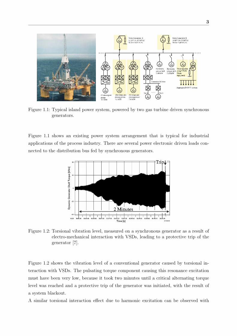
Figure 1.1: Typical island power system, powered by two gas turbine driven synchronousgenerators.
Figure 1.1 shows an existing power system arrangement that is typical for industrial
applications of the process industry. There are several power electronic driven loads con-
nected to the distribution bus fed by synchronous generators.
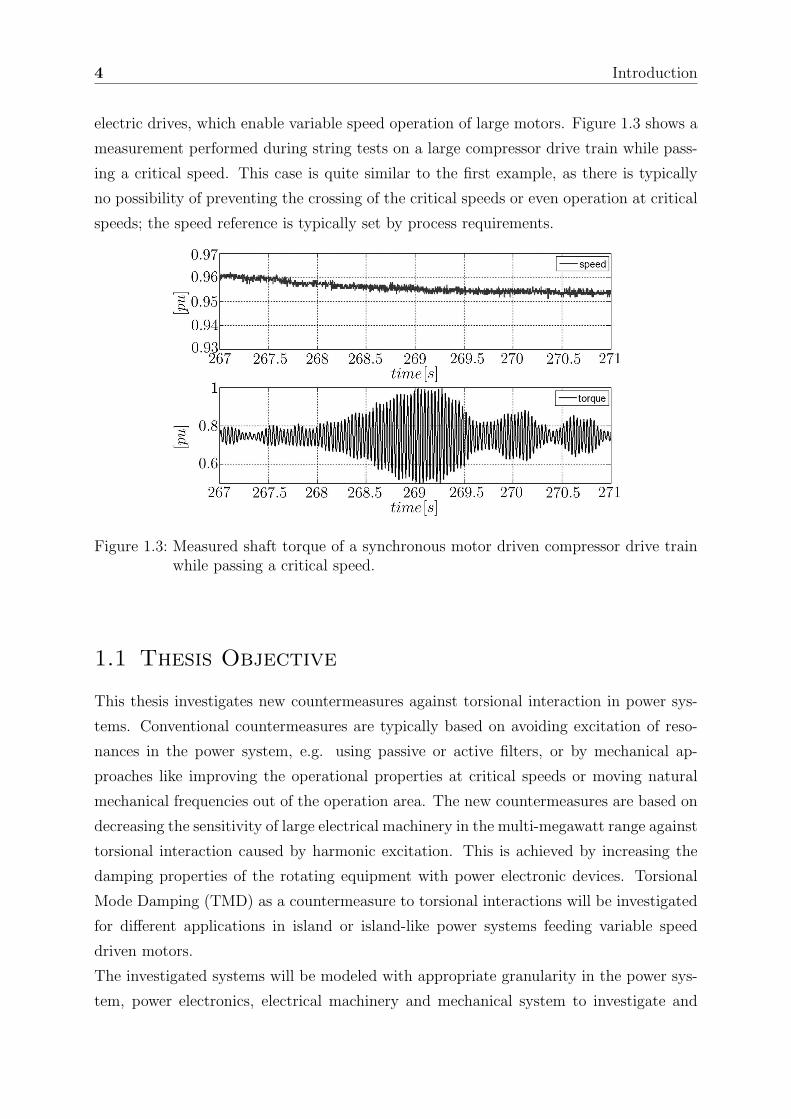
Figure 1.2: Torsional vibration level, measured on a synchronous generator as a result ofelectro-mechanical interaction with VSDs, leading to a protective trip of thegenerator [7].
Figure 1.2 shows the vibration level of a conventional generator caused by torsional in-
teraction with VSDs. The pulsating torque component causing this resonance excitation
must have been very low, because it took two minutes until a critical alternating torque
level was reached and a protective trip of the generator was initiated, with the result of
a system blackout.
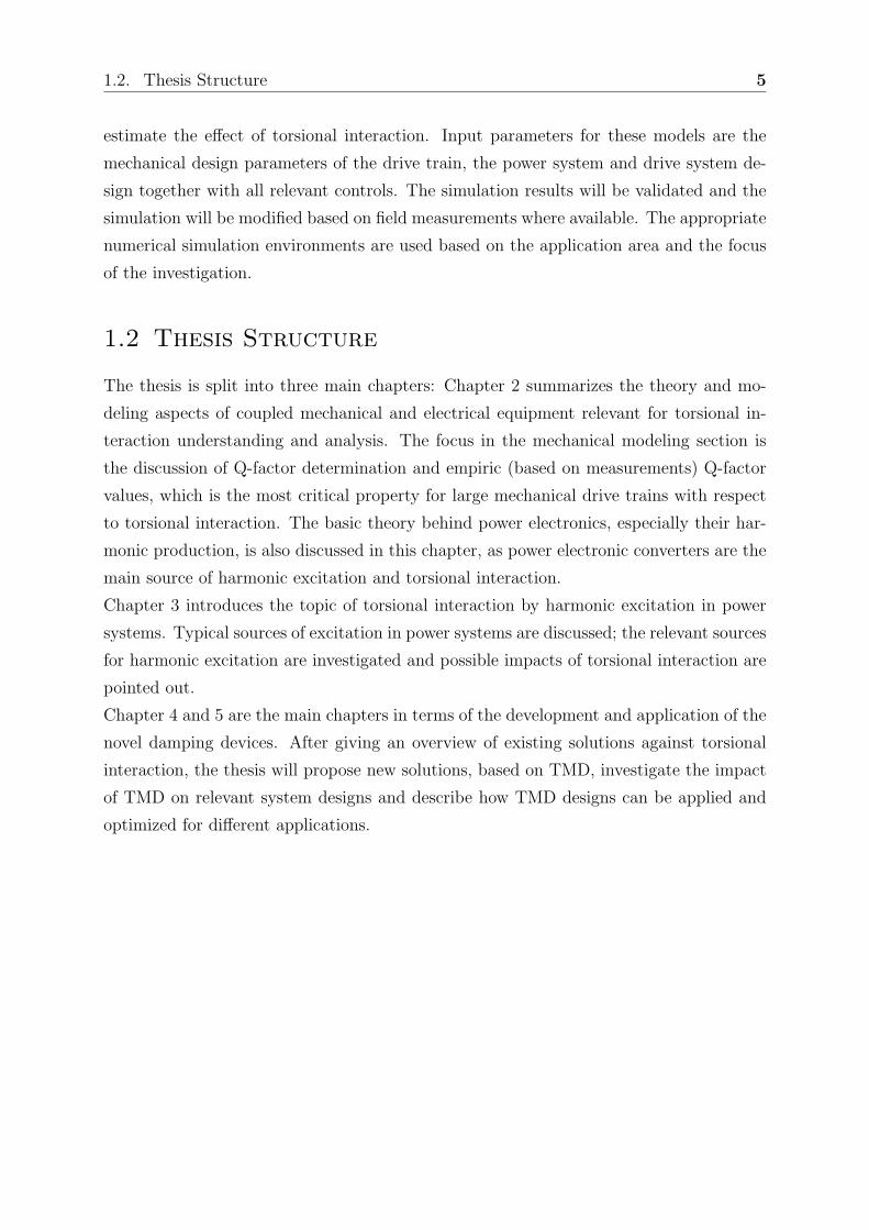
A similar torsional interaction effect due to harmonic excitation can be observed with
4 Introduction
electric drives, which enable variable speed operation of large motors. Figure 1.3 shows a
measurement performed during string tests on a large compressor drive train while pass-
ing a critical speed. This case is quite similar to the first example, as there is typically
no possibility of preventing the crossing of the critical speeds or even operation at critical
speeds; the speed reference is typically set by process requirements.
Figure 1.3: Measured shaft torque of a synchronous motor driven compressor drive trainwhile passing a critical speed.
1.1 Thesis Objective
This thesis investigates new countermeasures against torsional interaction in power sys-
tems. Conventional countermeasures are typically based on avoiding excitation of reso-
nances in the power system, e.g. using passive or active filters, or by mechanical ap-
proaches like improving the operational properties at critical speeds or moving natural
mechanical frequencies out of the operation area. The new countermeasures are based on
decreasing the sensitivity of large electrical machinery in the multi-megawatt range against
torsional interaction caused by harmonic excitation. This is achieved by increasing the
damping properties of the rotating equipment with power electronic devices. Torsional
Mode Damping (TMD) as a countermeasure to torsional interactions will be investigated
for different applications in island or island-like power systems feeding variable speed
driven motors.
The investigated systems will be modeled with appropriate granularity in the power sys-
tem, power electronics, electrical machinery and mechanical system to investigate and
1.2. Thesis Structure 5
estimate the effect of torsional interaction. Input parameters for these models are the
mechanical design parameters of the drive train, the power system and drive system de-
sign together with all relevant controls. The simulation results will be validated and the
simulation will be modified based on field measurements where available. The appropriate
numerical simulation environments are used based on the application area and the focus
of the investigation.
1.2 Thesis Structure
The thesis is split into three main chapters: Chapter 2 summarizes the theory and mo-
deling aspects of coupled mechanical and electrical equipment relevant for torsional in-
teraction understanding and analysis. The focus in the mechanical modeling section is
the discussion of Q-factor determination and empiric (based on measurements) Q-factor
values, which is the most critical property for large mechanical drive trains with respect
to torsional interaction. The basic theory behind power electronics, especially their har-
monic production, is also discussed in this chapter, as power electronic converters are the
main source of harmonic excitation and torsional interaction.
Chapter 3 introduces the topic of torsional interaction by harmonic excitation in power
systems. Typical sources of excitation in power systems are discussed; the relevant sources
for harmonic excitation are investigated and possible impacts of torsional interaction are
pointed out.
Chapter 4 and 5 are the main chapters in terms of the development and application of the
novel damping devices. After giving an overview of existing solutions against torsional
interaction, the thesis will propose new solutions, based on TMD, investigate the impact
of TMD on relevant system designs and describe how TMD designs can be applied and
optimized for different applications.


2Modeling and Component Aspects
Numerical simulation is an important tool in science and engineering. A model must
be sufficiently detailed but simple to understand and easy to manipulate. A model is
typically defined by what is considered relevant. The modeling basis relevant for torsional
interaction is described in the following chapter.
2.1 Mechanical Model
Torsional interaction (TI) is an interdisciplinary topic that involves mechanical and elec-
trical engineering, as it occurs often in mechanical systems, but for electrical reasons.
TI can occur in all drive train arrangements, but it is mainly critical for large rotating
machinery with low inherent damping properties. The mechanical damping at a natural
frequency is the critical parameter for the impact of TI. The determination of damping
parameters mainly based on empiric knowledge will be discussed.
The analysis of the torsional behavior is mandatory for large drive trains, e.g. [8]. The
basic theory and important tools will be discussed in this section. The main focus is on
understanding and evaluating the torsional interaction of large drive trains.
2.1.1 Single Mass System
A typical way to represent a mechanical system is to use discrete elements for mass (m),
spring (k) and damping (d). The masses of the system are concentrated on n masses,
7
8 Modeling and Component Aspects
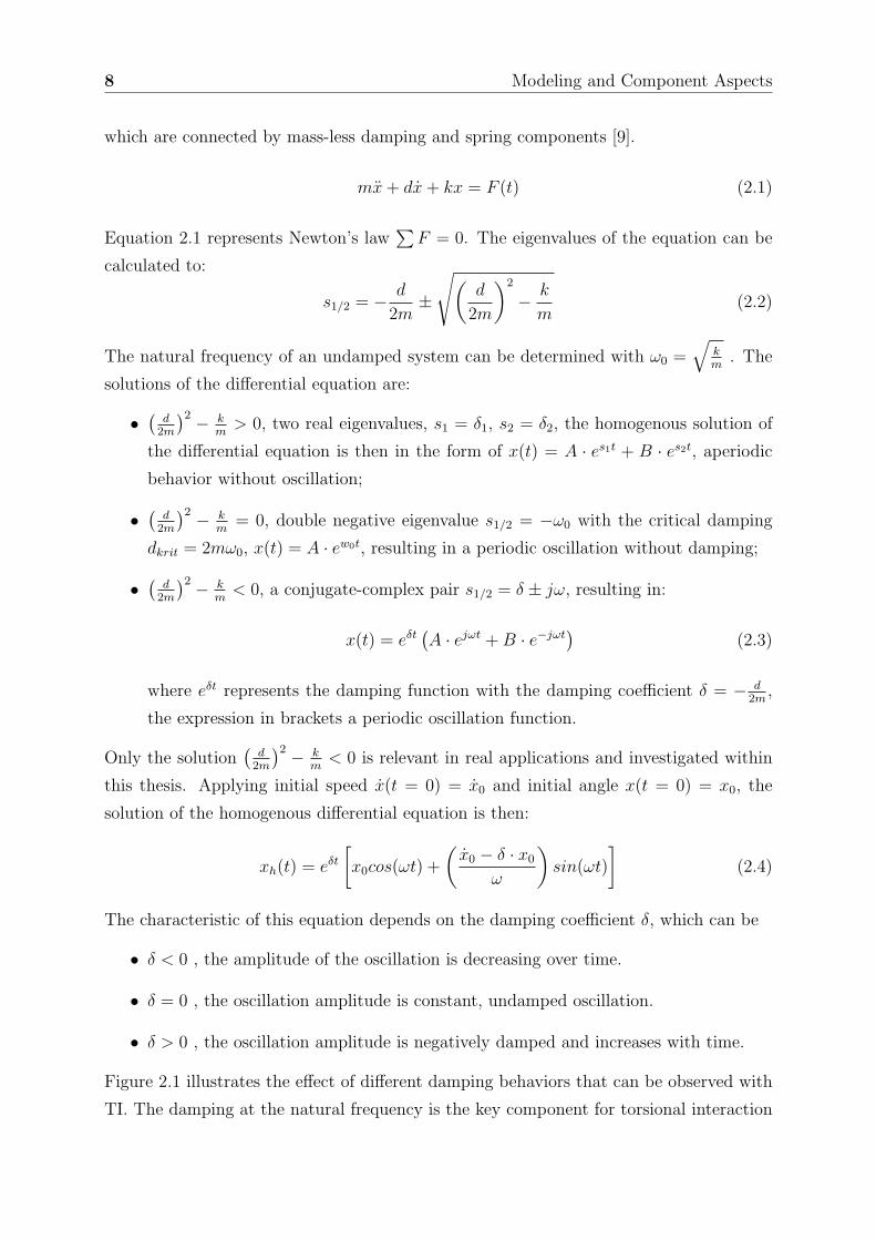
which are connected by mass-less damping and spring components [9].
mx + dx + kx = F (t) (2.1)
Equation 2.1 represents Newton’s law∑
F = 0. The eigenvalues of the equation can be
calculated to:
s1/2 = − d
2m±
√
(
d
2m
)2
− k
m(2.2)
The natural frequency of an undamped system can be determined with ω0 =√
km
. The
solutions of the differential equation are:
•(
d2m
)2 − km
> 0, two real eigenvalues, s1 = δ1, s2 = δ2, the homogenous solution of
the differential equation is then in the form of x(t) = A · es1t + B · es2t, aperiodic
behavior without oscillation;
•(
d2m
)2 − km
= 0, double negative eigenvalue s1/2 = −ω0 with the critical damping
dkrit = 2mω0, x(t) = A · ew0t, resulting in a periodic oscillation without damping;
•(
d2m
)2 − km
< 0, a conjugate-complex pair s1/2 = δ ± jω, resulting in:
x(t) = eδt(
A · ejωt + B · e−jωt)
(2.3)
where eδt represents the damping function with the damping coefficient δ = − d2m
,
the expression in brackets a periodic oscillation function.
Only the solution(
d2m
)2 − km
< 0 is relevant in real applications and investigated within
this thesis. Applying initial speed x(t = 0) = x0 and initial angle x(t = 0) = x0, the
solution of the homogenous differential equation is then:
xh(t) = eδt
[
x0cos(ωt) +
(
x0 − δ · x0
ω
)
sin(ωt)
]
(2.4)
The characteristic of this equation depends on the damping coefficient δ, which can be
• δ < 0 , the amplitude of the oscillation is decreasing over time.
• δ = 0 , the oscillation amplitude is constant, undamped oscillation.
• δ > 0 , the oscillation amplitude is negatively damped and increases with time.
Figure 2.1 illustrates the effect of different damping behaviors that can be observed with
TI. The damping at the natural frequency is the key component for torsional interaction

2.1. Mechanical Model 9
Figure 2.1: Impact of different damping coefficients on the resulting amplitude of oscilla-tion. Case 3 (δ > 0) is called negative damping (d < 0 ).
with large drive trains, as the mechanical inherent damping is very low at these frequen-
cies, and potentially negatively influenced by non-linearity in the power system, as will
be discussed in Chapter 2.1.3, 2.3 and 3.
2.1.2 Forced Oscillation
The partial solution of the differential equation depends on the type of external force F (t).
Distinguishing between non-periodic and periodic excitation will be made in the following
section. These are the main types of excitation for torsional interaction (Chapter 3).
NON-PERIODIC EXCITATION
Step function-like behavior as non-periodic excitation can be observed with TI, e.g. with
the torque response of a rotating drive train after an electrically close grid fault. A general
step function F (t) can be formulated with:
F (t) =
0 for t < 0
F for t ≥ 0(2.5)
10 Modeling and Component Aspects
The solution for the differential equation mx + dx + kx = F (t) can be formulated with
x(t = 0) = x0 and x(t = 0) = x0 and ζ = Fmω2
0to:
x(t) = eδt
(
(x0 − ζ)cos(ωt) +x − δ(x0 − ζ)
ωsin(ωt)
)
+ ζ (2.6)
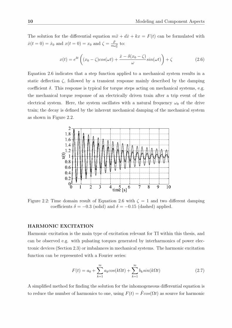
Equation 2.6 indicates that a step function applied to a mechanical system results in a
static deflection ζ, followed by a transient response mainly described by the damping
coefficient δ. This response is typical for torque steps acting on mechanical systems, e.g.
the mechanical torque response of an electrically driven train after a trip event of the
electrical system. Here, the system oscillates with a natural frequency ω0 of the drive
train; the decay is defined by the inherent mechanical damping of the mechanical system
as shown in Figure 2.2.
Figure 2.2: Time domain result of Equation 2.6 with ζ = 1 and two different dampingcoefficients δ = −0.3 (solid) and δ = −0.15 (dashed) applied.
HARMONIC EXCITATION
Harmonic excitation is the main type of excitation relevant for TI within this thesis, and
can be observed e.g. with pulsating torques generated by interharmonics of power elec-
tronic devices (Section 2.3) or imbalances in mechanical systems. The harmonic excitation
function can be represented with a Fourier series:
F (t) = a0 +∞∑
k=1
akcos(kΩt) +∞∑
k=1
bksin(kΩt) (2.7)
A simplified method for finding the solution for the inhomogeneous differential equation is
to reduce the number of harmonics to one, using F (t) = F cos(Ωt) as source for harmonic
2.1. Mechanical Model 11
excitation. The particular solution can be written for (ω0 6= Ω) as:
xp(t) =F
m
[
(Ω2 − ω20)[
cos(Ωt) − eδt(
δωsin(ωt) + cos(ωt)
)]
+ 2δ(
ω20
ωeδtsin(ωt) − Ωsin(Ωt)
)]
4δ2Ω2 + (ω20 − Ω2)
2
(2.8)
with x(t) = xh(t) + xp(t) (xh(t) - Equation 2.4). A second simplification is to neglect
the damping behavior of the mechanical system, which can be appropriate for large drive
trains; the differential equation is then reduced to mx + kx = F cos(Ωt). The solution for
ω0 = Ω can be written as:
x(t) = x0cos(ω0t) +x0
ω0
sin(ω0t) +F
2mω0
· t · sin(ω0t) (2.9)
Harmonic excitation at the natural frequency results in an increasing deflection, propor-
tional with time, dependent on amplitude of excitation F , inertia m and exposure time t.
Even small harmonic magnitudes e.g. interharmonics in the power system, can result in
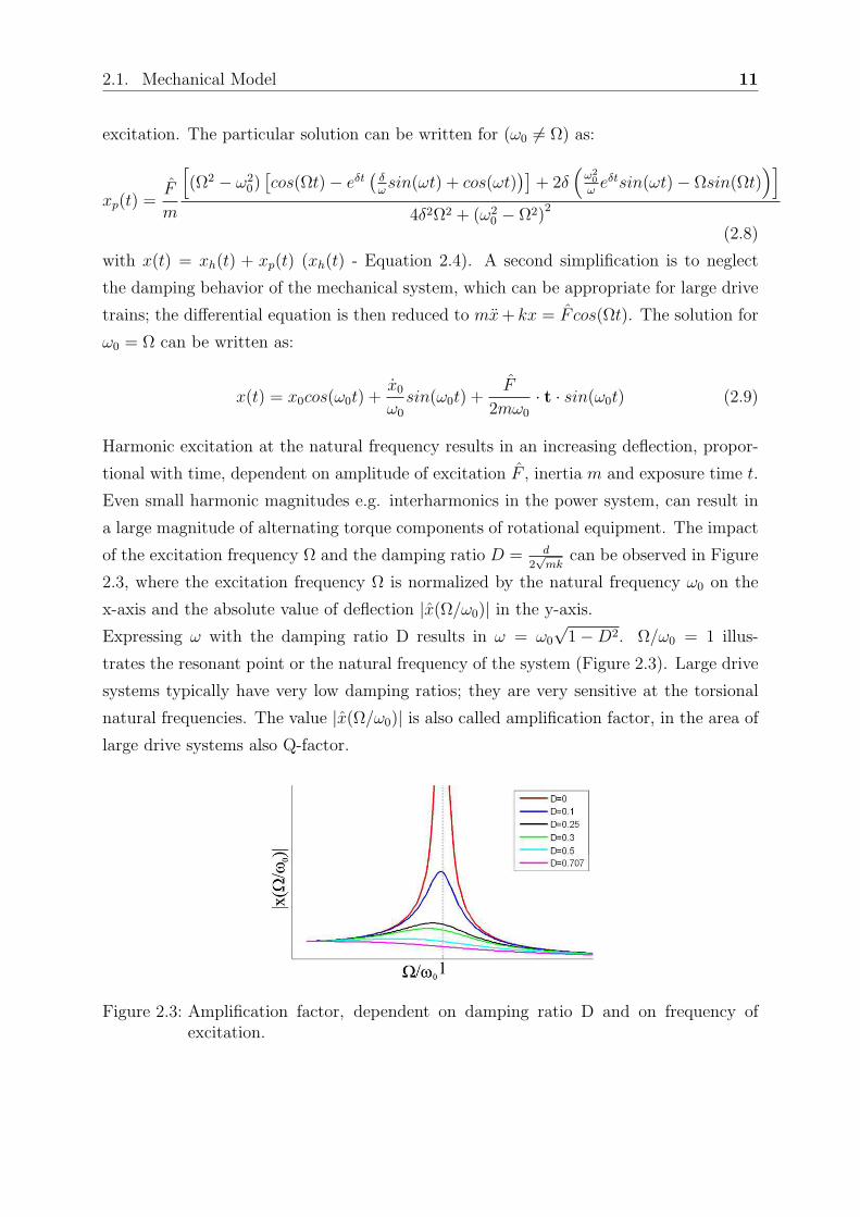
a large magnitude of alternating torque components of rotational equipment. The impact
of the excitation frequency Ω and the damping ratio D = d2√
mkcan be observed in Figure
2.3, where the excitation frequency Ω is normalized by the natural frequency ω0 on the
x-axis and the absolute value of deflection |x(Ω/ω0)| in the y-axis.
Expressing ω with the damping ratio D results in ω = ω0
√1 − D2. Ω/ω0 = 1 illus-
trates the resonant point or the natural frequency of the system (Figure 2.3). Large drive
systems typically have very low damping ratios; they are very sensitive at the torsional
natural frequencies. The value |x(Ω/ω0)| is also called amplification factor, in the area of
large drive systems also Q-factor.
Figure 2.3: Amplification factor, dependent on damping ratio D and on frequency ofexcitation.
12 Modeling and Component Aspects
2.1.3 Q-Factor Determination
The mechanical damping is the most critical parameter for torsional interaction with
large drive trains. The term ”damping” denotes the combined effect of influences due to
material damping, damping from windage, damping in bearings and electrical damping.
A quantitative assessment of the magnitude of damping has been possible only on the
basis of extensive measurements and tests [5]. The amplification factor caused by TI is
mainly critical close to the natural frequency. Figure 2.3 shows that the dynamic response
of mechanical systems is typically uncritical in frequency regions away from the resonance
point. Mechanical engineers prefer the expression amplification factor or Q-factor instead
of using, e.g., the damping ratio D, with Q = 12D
.
The Q-factor determination requires empiric knowledge; shaft material as well as shaft
shear stress have significant impact on this value, which makes it difficult to calculate the
effective Q-factor.
A convenient way to determine the amount of damping present in a system is to measure
the rate of decay of a free oscillation, e.g. after a trip of a mechanical system, where
the basic response of a mechanical system in the time domain is similar to Figure 2.2.
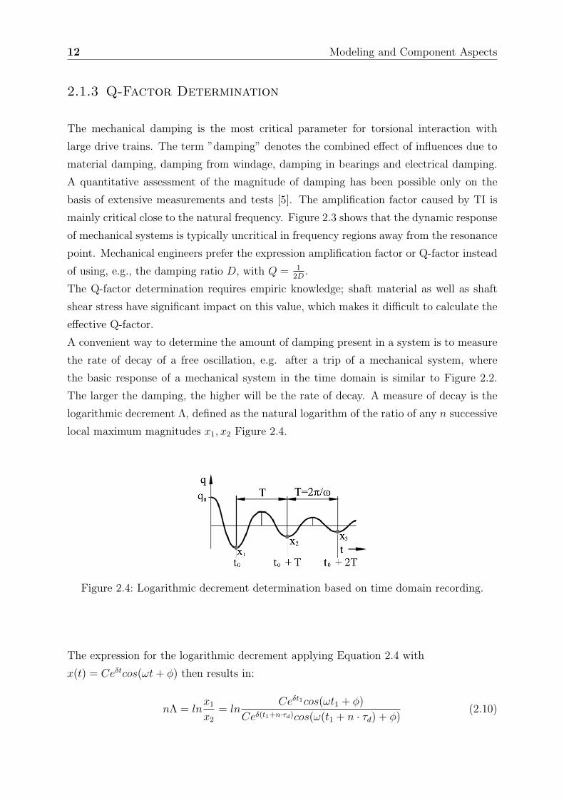
The larger the damping, the higher will be the rate of decay. A measure of decay is the
logarithmic decrement Λ, defined as the natural logarithm of the ratio of any n successive
local maximum magnitudes x1, x2 Figure 2.4.
Figure 2.4: Logarithmic decrement determination based on time domain recording.
The expression for the logarithmic decrement applying Equation 2.4 with
x(t) = Ceδtcos(ωt + φ) then results in:
nΛ = lnx1
x2
= lnCeδt1cos(ωt1 + φ)
Ceδ(t1+n·τd)cos(ω(t1 + n · τd) + φ)(2.10)
2.1. Mechanical Model 13
Using periodicity of the cos-function and the relation δ = −Dω0 and ω = ω0
√1 − D2
results in the logarithmic decrement equal to:
Λ =1
nln
x1
x2=
2πD√1 − D2
(2.11)
The Q-factor can be calculated to:
Q = 1/
(
2
√
Λ2
Λ2 + 4π2
)
(2.12)
Large drive trains typically have small damping values, Equation 2.11 can be simplified
to:
Λ = 2πD =π
Q=
1
nln
x1
x2
(2.13)
The Q-factor can therefore be calculated to:
Q =n · πlnx1
x2
(2.14)
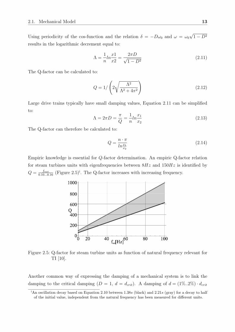
Empiric knowledge is essential for Q-factor determination. An empiric Q-factor relation
for steam turbines units with eigenfrequencies between 8Hz and 150Hz is identified by
Q = fnat
0.10...0.16(Figure 2.5)i. The Q-factor increases with increasing frequency.
Figure 2.5: Q-factor for steam turbine units as function of natural frequency relevant forTI [10].
Another common way of expressing the damping of a mechanical system is to link the
damping to the critical damping (D = 1, d = dcrit). A damping of d = (1%..2%) · dcrit
iAn oscillation decay based on Equation 2.10 between 1.38s (black) and 2.21s (gray) for a decay to halfof the initial value, independent from the natural frequency has been measured for different units.
14 Modeling and Component Aspects
results in a Q-factor value between 25 and 50 for synchronous motor-driven turbomachinery
(D = ddcrit
and Q = dcrit
2d), reported in [11]. Measurements (e.g. Figure 2.6) have shown
Q-factors between 100 and 1000 for large drive trains, which is more in line with Figure
2.5 and own experience during several measurements on large drive trains.
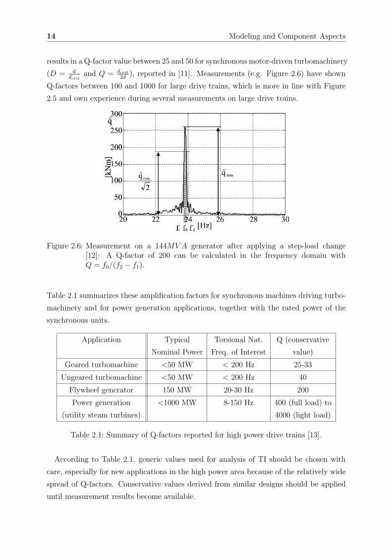
Figure 2.6: Measurement on a 144MV A generator after applying a step-load change[12]: A Q-factor of 200 can be calculated in the frequency domain withQ = f0/(f2 − f1).
Table 2.1 summarizes these amplification factors for synchronous machines driving turbo-
machinery and for power generation applications, together with the rated power of the
synchronous units.
Application Typical Torsional Nat. Q (conservative
Nominal Power Freq. of Interest value)
Geared turbomachine <50 MW < 200 Hz 25-33
Ungeared turbomachine <50 MW < 200 Hz 40
Flywheel generator 150 MW 20-30 Hz 200
Power generation <1000 MW 8-150 Hz 400 (full load) to
(utility steam turbines) 4000 (light load)
Table 2.1: Summary of Q-factors reported for high power drive trains [13].
According to Table 2.1, generic values used for analysis of TI should be chosen with
care, especially for new applications in the high power area because of the relatively wide
spread of Q-factors. Conservative values derived from similar designs should be applied
until measurement results become available.
2.1. Mechanical Model 15
The damping of a mechanical system can also be influenced by non-linear elements, e.g.
gearboxes. The Q-factor of geared drive trains is typically lower than ungeared systems;
a factor of two is mentioned in literature [11].
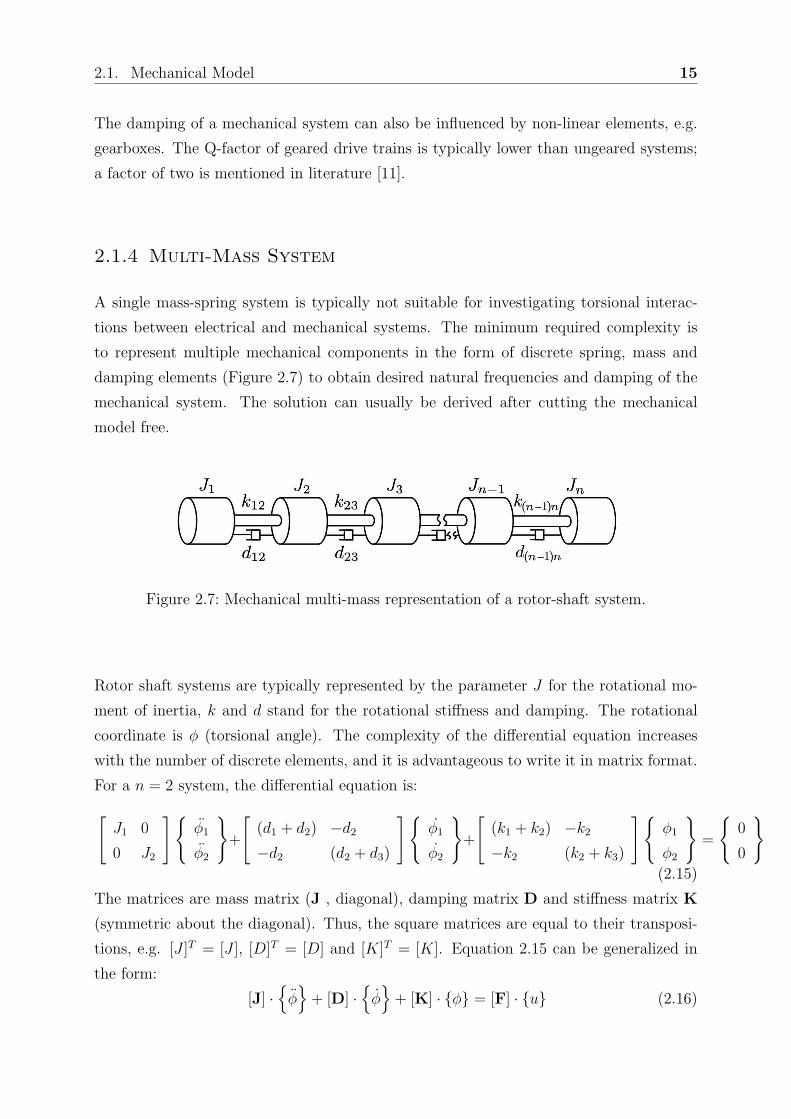
2.1.4 Multi-Mass System
A single mass-spring system is typically not suitable for investigating torsional interac-
tions between electrical and mechanical systems. The minimum required complexity is
to represent multiple mechanical components in the form of discrete spring, mass and
damping elements (Figure 2.7) to obtain desired natural frequencies and damping of the
mechanical system. The solution can usually be derived after cutting the mechanical
model free.
Figure 2.7: Mechanical multi-mass representation of a rotor-shaft system.
Rotor shaft systems are typically represented by the parameter J for the rotational mo-
ment of inertia, k and d stand for the rotational stiffness and damping. The rotational
coordinate is φ (torsional angle). The complexity of the differential equation increases
with the number of discrete elements, and it is advantageous to write it in matrix format.
For a n = 2 system, the differential equation is:
[
J1 0
0 J2
]
φ1
φ2
+
[
(d1 + d2) −d2
−d2 (d2 + d3)
]
φ1
φ2
+
[
(k1 + k2) −k2
−k2 (k2 + k3)
]
φ1
φ2
=
0
0
(2.15)
The matrices are mass matrix (J , diagonal), damping matrix D and stiffness matrix K
(symmetric about the diagonal). Thus, the square matrices are equal to their transposi-
tions, e.g. [J ]T = [J ], [D]T = [D] and [K]T = [K]. Equation 2.15 can be generalized in
the form:
[J] ·
φ
+ [D] ·
φ
+ [K] · φ = [F] · u (2.16)
16 Modeling and Component Aspects
where J can be written as:
J =
J1 0 . . . 0
0 J2 . . . 0...
.... . .
...
0 0 0 Jn
(2.17)
The Γ matrix (Equation 2.18) can be transformed into the damping matrix D in replacing
γx by dx, and into the stiffness matrix K in replacing γx by kx:
Γ =
(γ1 + γ2) −γ2 0 . . . 0 0
−γ2 (γ2 + γ3) −γ3 . . . 0 0...
......
.... . .
...
0 0 0 0 −γn−1 (γn−1 + γn)
(2.18)
The left side of Equation 2.16 is the second order differential equation representing the
mechanical system, and is given by the mechanical design of the system (see Chapter
2.1.1). Matrix F represents the external forces acting on the mechanical system, u repre-
sents the input vector of the system.
Equation 2.15 transformed into the well-known state space representation results in:
φ
φ
=
[
−D/J −K/J
I 0
]
·
φ
φ
+
[
I/J
0
]
·
0
y
=[
0 I]
·
φ
φ
(2.19)
with identity matrix I, rotational angle matrix φ =
[
φ1
φ2
]
, φ =
[
φ1
φ2
]
and φ =
[
φ1
φ2
]
. The
homogenous Equation 2.15 results in an input vector u of zero, which is not the general
case. The eigenvalues of a matrix are given by the values of the scalar parameter λ for
which there exist non-trivial solutions.
AΦ = λΦ (2.20)
The determinant (Equation 2.21) gives the characteristic equation with n solutions λ =
λ1, λ2, ..., λn, the eigenvalues of state matrix A.
Det(A − λI) = 0 (2.21)
2.1. Mechanical Model 17
The determination of the eigenvalues of the system is important for the modal analysis
(Chapter 2.1.5), as it represents the natural frequencies of the mechanical system. For
any eigenvalue λi the n-column vector Φi, which satisfies Equation 2.20, is called the right
eigenvector of A associated with the eigenvalue λi. The eigenvector has the form:
Φi =
Φ1,i
Φ2,i
...
Φn,i
It gives the ”mode shape” which is the relative activity of a state variable in a given mode
of the mechanical system (see Figure 2.8).
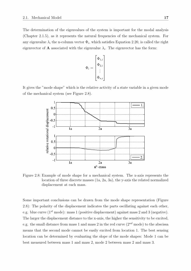
Figure 2.8: Example of mode shape for a mechanical system. The x-axis represents thelocation of three discrete masses (1a, 2a, 3a), the y-axis the related normalizeddisplacement at each mass.
Some important conclusions can be drawn from the mode shape representation (Figure
2.8): The polarity of the displacement indicates the parts oscillating against each other,
e.g. blue curve (1st mode): mass 1 (positive displacement) against mass 2 and 3 (negative).
The larger the displacement distance to the x-axis, the higher the sensitivity to be excited,
e.g. the small distance from mass 1 and mass 2 in the red curve (2nd mode) to the abscissa
means that the second mode cannot be easily excited from location 1. The best sensing
location can be determined by evaluating the slope of the mode shapes: Mode 1 can be
best measured between mass 1 and mass 2, mode 2 between mass 2 and mass 3.
18 Modeling and Component Aspects
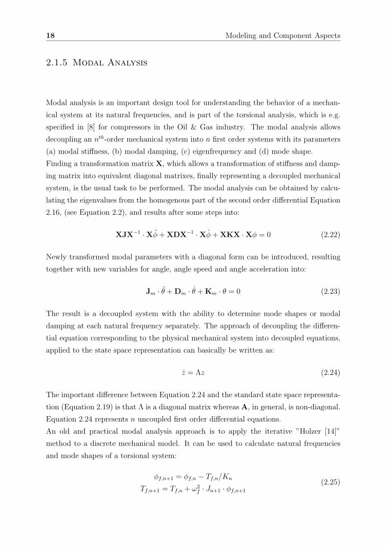
2.1.5 Modal Analysis
Modal analysis is an important design tool for understanding the behavior of a mechan-
ical system at its natural frequencies, and is part of the torsional analysis, which is e.g.
specified in [8] for compressors in the Oil & Gas industry. The modal analysis allows
decoupling an nth-order mechanical system into n first order systems with its parameters
(a) modal stiffness, (b) modal damping, (c) eigenfrequency and (d) mode shape.
Finding a transformation matrix X, which allows a transformation of stiffness and damp-
ing matrix into equivalent diagonal matrixes, finally representing a decoupled mechanical
system, is the usual task to be performed. The modal analysis can be obtained by calcu-
lating the eigenvalues from the homogenous part of the second order differential Equation
2.16, (see Equation 2.2), and results after some steps into:
XJX−1 · Xφ + XDX−1 · Xφ + XKX · Xφ = 0 (2.22)
Newly transformed modal parameters with a diagonal form can be introduced, resulting
together with new variables for angle, angle speed and angle acceleration into:
Jm · θ + Dm · θ + Km · θ = 0 (2.23)
The result is a decoupled system with the ability to determine mode shapes or modal
damping at each natural frequency separately. The approach of decoupling the differen-
tial equation corresponding to the physical mechanical system into decoupled equations,
applied to the state space representation can basically be written as:
z = Λz (2.24)
The important difference between Equation 2.24 and the standard state space representa-
tion (Equation 2.19) is that Λ is a diagonal matrix whereas A, in general, is non-diagonal.
Equation 2.24 represents n uncoupled first order differential equations.
An old and practical modal analysis approach is to apply the iterative ”Holzer [14]”
method to a discrete mechanical model. It can be used to calculate natural frequencies
and mode shapes of a torsional system:
φf,n+1 = φf,n − Tf,n/Kn
Tf,n+1 = Tf,n + ω2f · Jn+1 · φf,n+1
(2.25)
2.1. Mechanical Model 19
The starting condition of this algorithm is a unity amplitude at one end of the system,
φf,1 = 1 and progressively calculated speed and angular displacement at the other end.
The initial torque is calculated with Tf,1 = ω2f · J1. The quantities of concern are the
torsional displacement φ of each mass considered, the torque T carried by each shaft, in-
dex n represents the mass position Jn along the structure and ω = 2πf for the frequency
applied. Scanning with incremental frequencies f in the described iterative concept iden-
tifies the natural frequencies of the system:
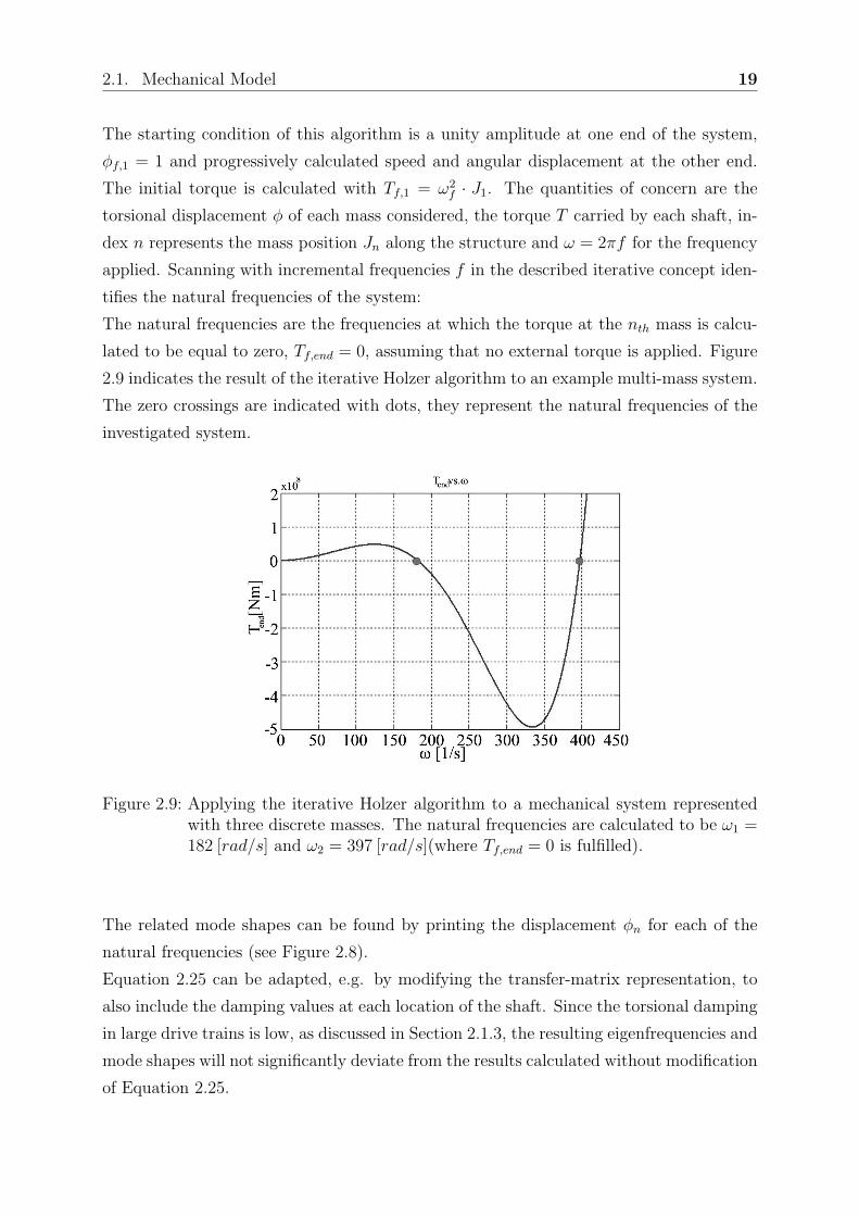
The natural frequencies are the frequencies at which the torque at the nth mass is calcu-
lated to be equal to zero, Tf,end = 0, assuming that no external torque is applied. Figure
2.9 indicates the result of the iterative Holzer algorithm to an example multi-mass system.
The zero crossings are indicated with dots, they represent the natural frequencies of the
investigated system.
Figure 2.9: Applying the iterative Holzer algorithm to a mechanical system representedwith three discrete masses. The natural frequencies are calculated to be ω1 =182 [rad/s] and ω2 = 397 [rad/s](where Tf,end = 0 is fulfilled).
The related mode shapes can be found by printing the displacement φn for each of the
natural frequencies (see Figure 2.8).
Equation 2.25 can be adapted, e.g. by modifying the transfer-matrix representation, to
also include the damping values at each location of the shaft. Since the torsional damping
in large drive trains is low, as discussed in Section 2.1.3, the resulting eigenfrequencies and
mode shapes will not significantly deviate from the results calculated without modification
of Equation 2.25.

20 Modeling and Component Aspects
2.1.6 Model Reduction
Simulation lives from simplification. It is not necessary to use a finite element represen-
tation of the mechanical model for the analysis of TI, as the frequencies of interest are
typically up to or around the synchronous frequency. It is therefore recommended to re-
duce complex mechanical systems, so as to be suitable for application in combined electro-
mechanical simulation environments, to limit the computational effort required with an
appropriate granularity of the mechanical representation. There are several methods avail-
able for a degree-of-freedom reduction for torsional systems. An iterative method is the
reduction approach introduced by RIVIN [15] and DI [16]. A torsional model with a high
degree of freedom can be subdivided into subsystems with one of the two representations
indicated in Figure 2.10: either a subsystem including two torsional springs associated
with one rotational inertia Jk (type a) or two inertias connected by one torsional spring
kTk (type b). A nth order torsional system can than be split into n subsystems of type a
and (n − 1) subsystems of type b.
Figure 2.10: Two different types of subsystem of a reduced torsional model.
The eigenfrequencies for all subsystems k = 1, 2, ..., n − 1 and kT0 = kT (n+1) = 0 can be
calculated based on Equation 2.2 with:
ω2ak =
kT (k−1)+kTk
Jk; ω2
bk = kTk(Jk+Jk+1)
JkJk+1; (2.26)
Equation 2.26 results in 2n−1 different natural frequencies for the subsystems. The max-
imum of all identified subsystem natural frequencies represents the most rigid subsystem:
ω2k−max = MAXk=1..n
[
ω2ak, ω
2bk
]
(2.27)
A partial model reduction will be applied to the subsystem identified in Equation 2.27;
it will be split to the closest connected subsystems. Therefore, after each reduction step
the degree of freedom of the torsional system will decrease, until the desired degree of
freedom or maximum remaining eigenfrequency is reached.
2.2. Electrical Machine 21
2.2 Electrical Machine
The electrical machine is the interface between the electrical power system and the me-
chanical drive train. The two most important ways of applying torque with electrical
machinery in the high power area are: (a) asynchronous, stator and rotor have different
”rotational” speeds, a field is induced from stator to rotor or from rotor to stator; and (b)
synchronous, flux linkage between stator and rotor, generated from independent sources
in stator and rotor, e.g. by current sources. The electrical machine models used in this
thesis are represented as quasi-stationary; the electromagnetic transients are typically
much faster than the mechanical time constants involved with torsional dynamics.
2.2.1 Induction Machine
The most commonly used small to medium sized motor is the induction or asynchronous
machine because of the clear advantages: simple and robust machine design, self start-
ability, and comparably low initial cost. Induction machines in the high power range are
rare, but they exist [17]. More reactive power consumption and higher losses compared
to synchronous machines limit applications in the multi-megawatt range.
One special example of an induction machine in large drive trains is the doubly fed induc-
tion machine (DFIM) used with variable speed wind turbines. The design varies slightly
from the standard induction machine in that it has access to the rotor windings to ma-
nipulate the effective rotor current frequency. The dynamic behavior of a field-oriented,
controlled, doubly fed induction machine is close to that of a synchronous machine as
long as the frequency of interest is within the bandwidth of the current control, which is
at least around 50Hz.
A conventional induction machine acts on pulsating torque components in the lower fre-
quency range with a nearly proportional torque-slip characteristic, providing additional
damping of non-fundamental frequency components to the mechanical drive train. The
dynamic characteristic of an induction machine derived in [18] results in:
M +
(
2sk +φ
2Ω2
)
MΩ +
(
(s2k + s2)Ω2 +
φsk
2
)
M = 2MksksΩ2 (2.28)
The variables are torque M , synchronous speed Ω, angular motor speed φ, slip s and the
two parameters defining the torque-slip characteristic are the stall torque Mk and stall
slip sk.

22 Modeling and Component Aspects
Equation 2.28 linearized and reduced to the static case (φ = 0, M = 0, M = 0) results
in:
M = 2Mksks
s2k + s2
(2.29)
the well-known Kloss equation.
Figure 2.11: Damping effect of the slip of an induction machine, dependent on the fre-quency of the pulsating torque components. The different colors indicatedifferent modulation amplitudes, ’*’,’o’ and ’+’ different inertia values.
Figure 2.11 illustrates the effect of the pulsating torque frequency on the damping effect
introduced by the slip of an induction machine based on Equation 2.28. The damping
effect of the slip reduces with higher pulsating torque frequency. The amplitude of the
pulsating torque has limited effect on the damping, as long as the stall torque is not
reached. This curve was derived as an electrical torque response to a change in machine
speed (Figure 2.12):
De(f) =∆T (f)
∆ω(f)(2.30)
The frequency axis (Figure 2.11) is related to the rotational frame of the electrical ma-
chine, the effective pulsating torque components have to be calculated as sideband of the
nominal electrical frequency. The slip value is equivalent to the losses of the induction ma-
chine; large drive trains have comparably low slip values, resulting in a large torque/slip
ratio, representing a relatively stiff electro-mechanical connection with limited damping
property.
2.2. Electrical Machine 23
2.2.2 Synchronous Machine
The synchronous machine is the most important electrical machine for power generation,
but also for motoring of high power loads. The conventional synchronous design allows
the control of reactive power by adjustment of the excitation voltage, and more impor-
tant for high power applications, a higher efficiency compared to the induction design
[19]. (a) Slip-ring or (b) brushless and (c) permanent magnet excitation systems are the
main solutions for the exciter system. Disadvantages are lower reliability, especially for
higher operational speeds with slip rings (a) or a more complex motor construction due
to the presence of two windings on the stator and for the rotating diodes (b) [17]. The
permanent magnet synchronous machine (c) is the main driver for the utilization of the
synchronous machinery in the lower multi-megawatt power range, e.g. in wind turbines,
with higher complexity for the control of this type of machine. The rotor always rotates
with synchronous speed, resulting in a start-up challenge, which can be mitigated by using
a starting inverter or a starting (induction) machine or winding. Using induction-windings
results in well-known torsional interaction during start-up, caused by a match between
pulsating torques and natural frequencies of the drive train because of the typical asym-
metrical rotor design, salient poles generating torque output as a function of the rotor
position. The frequency of the torque pulsation is the difference in frequency between the
stator and the rotor, known as slip speed for induction type machines. The net result of
this is a torque pulsation that occurs at twice the slip frequency, which is defined as:
fslip = f1ns − n
ns
(2.31)
to be:
Tpuls(n) = 2fslip = 2f1ns − n
ns
(2.32)
The pulsating torque (Equation 2.32) can be eliminated with using a starting inverter,
which is an elegant but rather expensive means of reducing the motor torques only during
start-up, e.g. as described in Chapter 2.3. This type of torsional interaction will not be
discussed further in this document. A direct startup of a synchronous machine in the
described way is relatively seldom.
The torque of a synchronous machine is nearly sinusoidal. The rotor lags behind the
rotating field with the (electrical) angle Θ.
T = Tmaxsin(Θ) (2.33)
24 Modeling and Component Aspects
The relation torque/angle is the same as a spring characteristic of the air-gap torque.
Some design modifications allow uncritical operation by adding damping elements to the
characteristics of the synchronous machine [20]:
1. Asynchronous damping moment, similar to the induction machine where the rotor
slips to the stator winding. The asynchronous damping moment provides the major
contribution for the damping torque, mainly for higher load levels; but it is very
low for no-load operation.
2. The synchronous damping moment, caused by pulsating currents in the armature
because of angular oscillation; this term is always negative, relevant for low load
operation, where a continuous oscillation can be observed for large synchronous
generators.
3. Alternating damping moment, because of interaction between armature and (elec-
trical) angle, positive for generation, negative for motoring.
The positive damping of the asynchronous damping (1) has the highest influence on
the damping of the synchronous machine, and is typically amplified by the mechanical
damping provided by the load characteristic, typically higher damping for higher load
operation. The resistance in the damping winding is usually higher compared to that in
the induction machine design, resulting in a smaller overall damping effect; a factor 10
times smaller has been reported in [4].
2.2.3 Torque Modulation
Electrical machinery converts electrical into mechanical, typically rotational, energy or
vice versa. Rotating quantities like torque can be expressed in terms of stationary, but
also in terms of rotational frame. The Park coordinate transformation can be used to link
harmonic currents e.g. produced in power converters to pulsating torque components.
The impact of the non-fundamental frequency components on the mechanical drive train
depends on the dynamic performance of the electrical and mechanical design. The rel-
evant electrical dynamics have already been discussed in Sections 2.2.1 and 2.2.2. The
mechanical dynamics are influenced by the drive train inertia J , which is accelerated by
the imbalance between the applied air-gap and mechanical torque:
Tm − Te = Jdωm
dt(2.34)
2.2. Electrical Machine 25
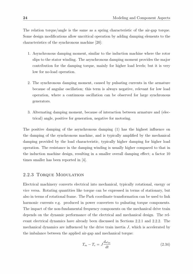
The full electromechanical relationship can be identified in Figure 2.12.
Figure 2.12: Equation of motion for an electromechanical system: Tm applies to the me-chanical torque, K12 represents the mechanical stiffness coefficient, D the me-chanical damping coefficient, and Ks the synchronization torque coefficient.
The equation of motion can be written to:
∆ω =1
J(K12∆δ − D∆ω − Te) (2.35)
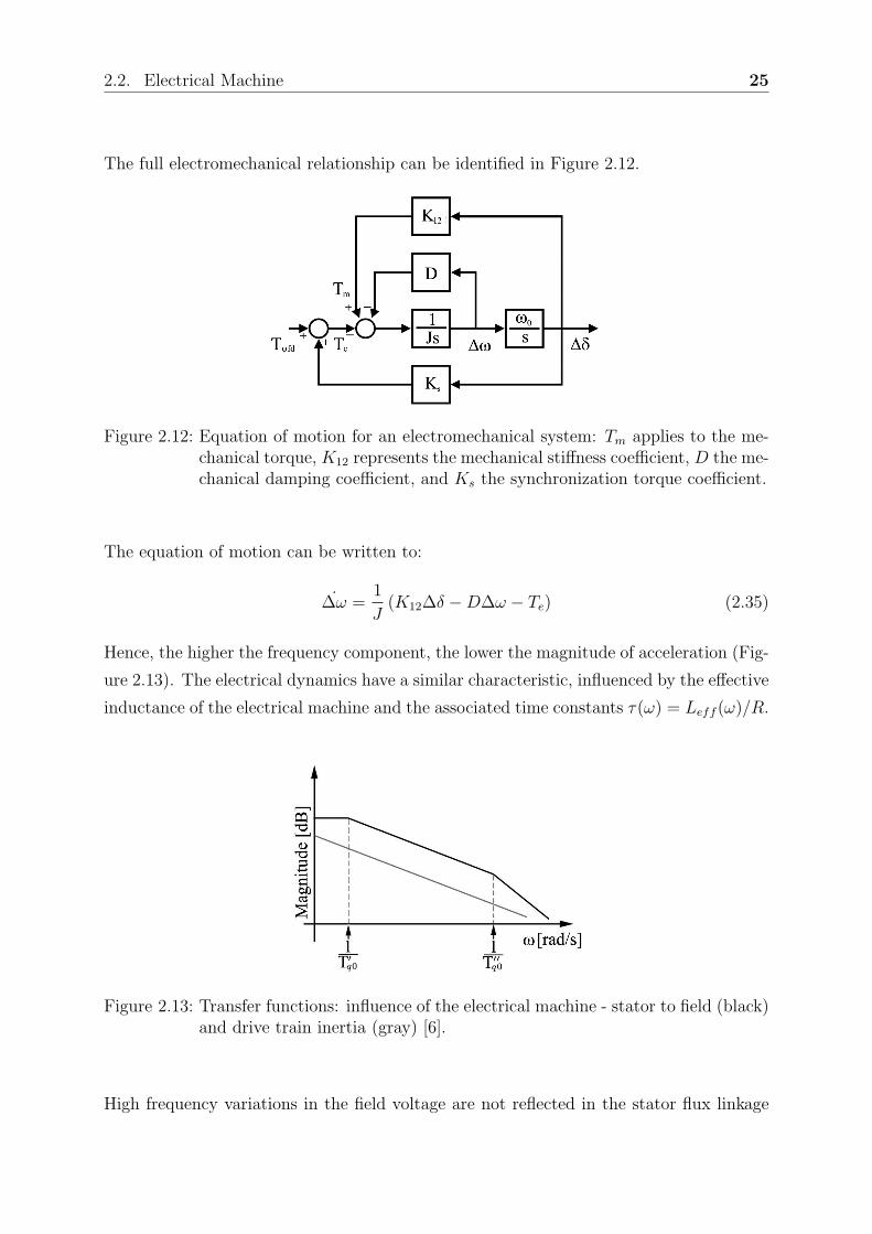
Hence, the higher the frequency component, the lower the magnitude of acceleration (Fig-
ure 2.13). The electrical dynamics have a similar characteristic, influenced by the effective
inductance of the electrical machine and the associated time constants τ(ω) = Leff (ω)/R.
Figure 2.13: Transfer functions: influence of the electrical machine - stator to field (black)and drive train inertia (gray) [6].
High frequency variations in the field voltage are not reflected in the stator flux linkage

26 Modeling and Component Aspects
and hence other stator quantities, they do not result in considerable pulsating torque
components [6].
2.3 Power Electronic Devices
Power electronic devices play an increasing role in modern electrification scenarios. They
allow higher flexibility and higher efficiency, e.g. with variable speed operation in drive
train applications replacing conventional fixed speed electrical and non-electrical drives
(e.g. gas-turbines). The Electric Power Research Institute (EPRI) estimates, that 60%
to 65% of generated electrical energy in the US are consumed in motor drives. Most of
the machines operate at light load most of the time. Motor efficiency can be improved
by as much as 30% by reduced flux operation instead of operating with rated flux [21].
Power electronics is also widely used in transmission, e.g. for High Voltage DC (HVDC)-
Transmission or Flexible AC Transmission (FACTS). The focus in this document is (a)
the impact of power electronic designs used in high power applications with respect to TI,
and (b) the use of different designs for the active damping approach (Chapter 5). Two
principle converter designs are relevant in applications of high power electronics:
1. Voltage source converters, operating with a DC-voltage always with one polarity
and supported by a DC-capacitor. The power reversal takes place through reversal
of the DC-current polarity.
2. Current source converters, operating with a DC-current always at one polarity and
supported by a DC-reactor. The power reversal takes place through reversal of the
DC-voltage polarity.
Figure 2.14 summarizes the two principle design options and indicates fundamental differ-
ences in the capability of the design. A second way of distinguishing the power electronic
devices used in the high power area is to distinguish at the semiconductor level between
a self-commutated and line-commutated inverter type. The valves of Line-Commutated
Inverter (LCI) have only turn-on control capability; turn-off depends on the current zero
crossing as per circuit and system conditions. The valves of a self-commutated converter
have turn-on and turn-off capability. Devices such as Gate Turn-Off Thyristor (GTO),
Integrated Gate Bipolar Transistor (IGBT) and Integrated Gate-Commutated Thyristor
(IGCT) and similar devices have turn-on and turn-off capability. A property comparison
of the main types of power electronic converters, relevant for high power applications, is
summarized in Table 2.2. It explains why line commutated converters are still attractive

2.3. Power Electronic Devices 27
Figure 2.14: (a) Voltage source converter design, (b) Current source converter design [22].
Characteristic Line-Commutated Self-CommutatedDesign Options Current Source Voltage- or Current Source
Dynamic Performance Medium HighRating 1-80 MW Up to 8 MW per Module
Efficiency High MediumReliability High Medium
System Cost Low HighComplexity Low High
Reactive Power Consumption Consumption or ProductionPower Quality Low-Medium Medium-High
Torsional Interaction High MediumFootprint Low Medium
Table 2.2: Relative comparison between line-commutated and self-commutated invertertype [23–25].
for high power applications. Switching devices always produce harmonics, which can ex-
cite torsional natural frequencies, independent from the power electronics design, if the
generated harmonics are in coincidence with one of the torsional natural frequencies of
the mechanical drive train. It is essential to know the frequency and amplitude of the
generated harmonics to estimate the impact on the torsional behavior of the system.
Conventional countermeasures to the torsional interaction with power electronic devices
are based on increasing the frequency of low order torque harmonics (e.g. by increasing the
converter switching frequency) or decreasing their amplitude (e.g. by multi-level converter
topologies or by increasing the effective commutation inductance of load-commutated
converter). The fundamentals for harmonics production are discussed in the following
chapters.
28 Modeling and Component Aspects
2.3.1 Line-Commutated Inverter (LCI)
Line-commutated inverters are well known in the high power area because of their simplicity,
proven reliability and practically unlimited output power, but also because of limited dy-
namic performance. Typical LCIs in the high power range are based on a 6 or 12-pulse
design. It will be shown in the following subsections, that the pulse number significantly
influences the location and amplitude of the produced harmonics and interharmonics.
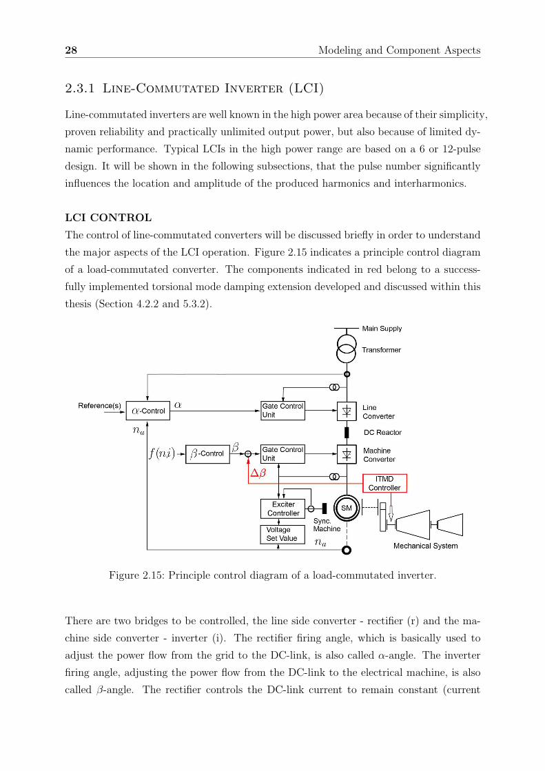
LCI CONTROL
The control of line-commutated converters will be discussed briefly in order to understand
the major aspects of the LCI operation. Figure 2.15 indicates a principle control diagram
of a load-commutated converter. The components indicated in red belong to a success-
fully implemented torsional mode damping extension developed and discussed within this
thesis (Section 4.2.2 and 5.3.2).
Figure 2.15: Principle control diagram of a load-commutated inverter.
There are two bridges to be controlled, the line side converter - rectifier (r) and the ma-
chine side converter - inverter (i). The rectifier firing angle, which is basically used to
adjust the power flow from the grid to the DC-link, is also called α-angle. The inverter
firing angle, adjusting the power flow from the DC-link to the electrical machine, is also
called β-angle. The rectifier controls the DC-link current to remain constant (current
2.3. Power Electronic Devices 29
source converter type). Its value depends on the desired torque level of the connected
electrical machine; a superior speed control sets the current reference. The steady state
and dynamic behavior of the converter is highly nonlinear [26]. A change in the firing an-
gle command becomes delayed before becoming effective in the power circuit; the delay is
between 0ms..206ms for a 6-pulse system with 50Hz grid frequency. A typical approach is
to approximate the delay with TT = 1.67ms for the given control design example (Figure
2.16). The control dynamics are influenced by the time constant given by the commuta-
tion inductance, τ =∑ Lk
Rand by the period firing delay between 0...Tpulse, higher pulse
numbers allow faster controllability. The focus in this section is mainly on the current
control loop controlling the α-angle. This loop can influence the operation of the damping
loop, which will be discussed in Section 5.3.2.
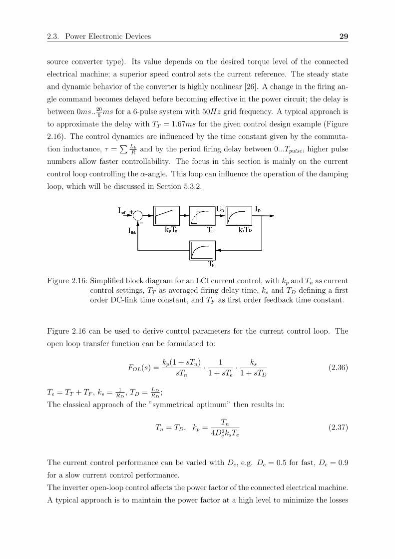
Figure 2.16: Simplified block diagram for an LCI current control, with kp and Tn as currentcontrol settings, TT as averaged firing delay time, ks and TD defining a firstorder DC-link time constant, and TF as first order feedback time constant.
Figure 2.16 can be used to derive control parameters for the current control loop. The
open loop transfer function can be formulated to:
FOL(s) =kp(1 + sTn)
sTn
· 1
1 + sTe
· ks
1 + sTD
(2.36)
Te = TT + TF , ks = 1RD
, TD = LD
RD;
The classical approach of the ”symmetrical optimum” then results in:
Tn = TD, kp =Tn
4D2cksTe
(2.37)
The current control performance can be varied with Dc, e.g. Dc = 0.5 for fast, Dc = 0.9
for a slow current control performance.
The inverter open-loop control affects the power factor of the connected electrical machine.
A typical approach is to maintain the power factor at a high level to minimize the losses
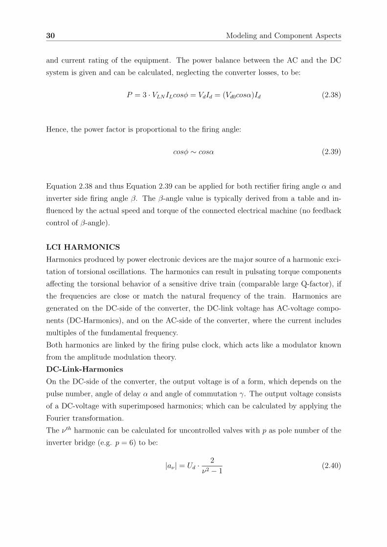
30 Modeling and Component Aspects
and current rating of the equipment. The power balance between the AC and the DC
system is given and can be calculated, neglecting the converter losses, to be:
P = 3 · VLNILcosφ = VdId = (Vd0cosα)Id (2.38)
Hence, the power factor is proportional to the firing angle:
cosφ ∼ cosα (2.39)
Equation 2.38 and thus Equation 2.39 can be applied for both rectifier firing angle α and
inverter side firing angle β. The β-angle value is typically derived from a table and in-
fluenced by the actual speed and torque of the connected electrical machine (no feedback
control of β-angle).
LCI HARMONICS
Harmonics produced by power electronic devices are the major source of a harmonic exci-
tation of torsional oscillations. The harmonics can result in pulsating torque components
affecting the torsional behavior of a sensitive drive train (comparable large Q-factor), if
the frequencies are close or match the natural frequency of the train. Harmonics are
generated on the DC-side of the converter, the DC-link voltage has AC-voltage compo-
nents (DC-Harmonics), and on the AC-side of the converter, where the current includes
multiples of the fundamental frequency.
Both harmonics are linked by the firing pulse clock, which acts like a modulator known
from the amplitude modulation theory.
DC-Link-Harmonics
On the DC-side of the converter, the output voltage is of a form, which depends on the
pulse number, angle of delay α and angle of commutation γ. The output voltage consists
of a DC-voltage with superimposed harmonics; which can be calculated by applying the
Fourier transformation.
The νth harmonic can be calculated for uncontrolled valves with p as pole number of the
inverter bridge (e.g. p = 6) to be:
|aν | = Ud ·2
ν2 − 1(2.40)
2.3. Power Electronic Devices 31
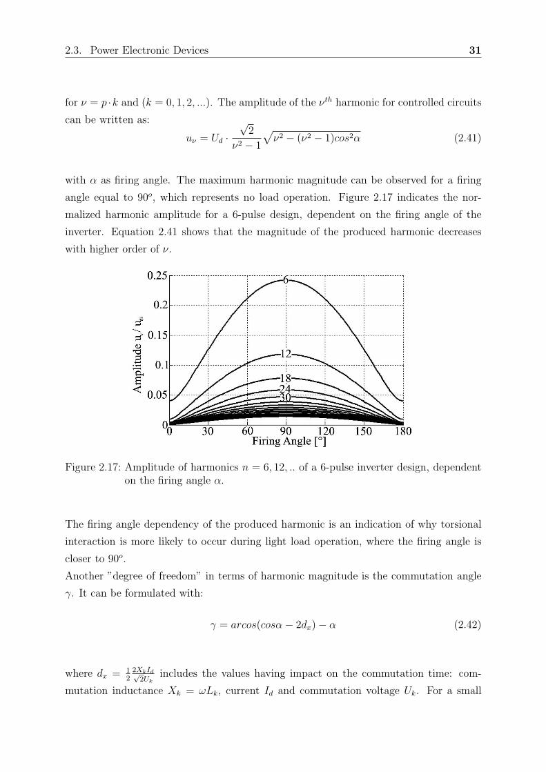
for ν = p ·k and (k = 0, 1, 2, ...). The amplitude of the νth harmonic for controlled circuits
can be written as:
uν = Ud ·√
2
ν2 − 1
√
ν2 − (ν2 − 1)cos2α (2.41)
with α as firing angle. The maximum harmonic magnitude can be observed for a firing
angle equal to 90o, which represents no load operation. Figure 2.17 indicates the nor-
malized harmonic amplitude for a 6-pulse design, dependent on the firing angle of the
inverter. Equation 2.41 shows that the magnitude of the produced harmonic decreases
with higher order of ν.
Figure 2.17: Amplitude of harmonics n = 6, 12, .. of a 6-pulse inverter design, dependenton the firing angle α.
The firing angle dependency of the produced harmonic is an indication of why torsional
interaction is more likely to occur during light load operation, where the firing angle is
closer to 90o.
Another ”degree of freedom” in terms of harmonic magnitude is the commutation angle
γ. It can be formulated with:
γ = arcos(cosα − 2dx) − α (2.42)
where dx = 12
2XkId√2Uk
includes the values having impact on the commutation time: com-
mutation inductance Xk = ωLk, current Id and commutation voltage Uk. For a small
32 Modeling and Component Aspects
commutation angle γ, the harmonic magnitude increases with increasing firing angle α
until α >= 90o, see Figure 2.17. For a constant angle α, the harmonics decrease with
increasing commutation angle γ and reach a first minimum at, approximately γ = π/ν,
e.g. for a 6-pulse design at γ = 30o.
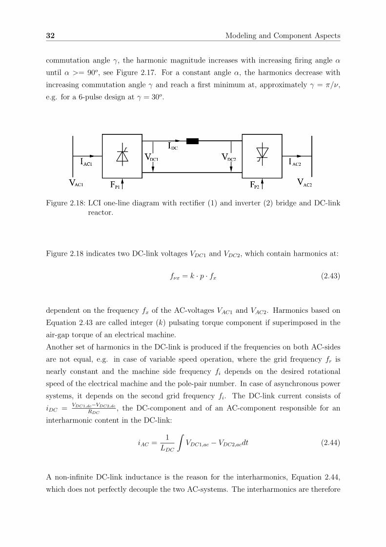
Figure 2.18: LCI one-line diagram with rectifier (1) and inverter (2) bridge and DC-linkreactor.
Figure 2.18 indicates two DC-link voltages VDC1 and VDC2, which contain harmonics at:
fνx = k · p · fx (2.43)
dependent on the frequency fx of the AC-voltages VAC1 and VAC2. Harmonics based on
Equation 2.43 are called integer (k) pulsating torque component if superimposed in the
air-gap torque of an electrical machine.
Another set of harmonics in the DC-link is produced if the frequencies on both AC-sides
are not equal, e.g. in case of variable speed operation, where the grid frequency fr is
nearly constant and the machine side frequency fi depends on the desired rotational
speed of the electrical machine and the pole-pair number. In case of asynchronous power
systems, it depends on the second grid frequency fi. The DC-link current consists of
iDC =VDC1,dc−VDC2,dc
RDC, the DC-component and of an AC-component responsible for an
interharmonic content in the DC-link:
iAC =1
LDC
∫
VDC1,ac − VDC2,acdt (2.44)
A non-infinite DC-link inductance is the reason for the interharmonics, Equation 2.44,
which does not perfectly decouple the two AC-systems. The interharmonics are therefore

2.3. Power Electronic Devices 33
present in both AC-systems. The resulting interharmonics are in the form:
fν 12 = |k · p · f1 ± m · p · f2| (2.45)
The frequencies f1,f2 of both AC-systems are multiplied with the independent integer
variables k,m = 1, 2, 3, ... and the effective pulse number of the utilized converter bridge
p. The harmonics, also called non-integer harmonics, are the main reason for TI between
power electronics-driven systems and conventional rotating machinery, which transform
them into pulsating torque components. Some of them are in the lower frequency range,
and they vary with varying frequency, so that a large number of frequencies can be
excited by this set of harmonics (see also Figure 2.19). Equation 2.45 will be derived
in the next subchapter. A design criterion for modern LCIs in high power applications
is the production of interharmonics with magnitudes as low as possible, less than one
percent of the nominal power can be achieved. But this can still cause relevant torsional
excitation [27]. This low level of pulsating torque production has also been observed in
air-gap torque measurements during tests performed on a 30MW O&G train driven by
an LCI.
AC-Side Harmonics
Current harmonics produced on the AC-side of the converter can be derived from the
typically rectangular like current shape, as shown in [22]. The generated harmonics are
in the order of:
n = p · k ± 1 (2.46)
where n is the harmonic order, k = 1, 2, 3, ... and p the pulse number of the inverter
bridge. Higher harmonics and higher pulse numbers result in lower magnitudes; the nth
harmonic has an amplitude of:
In =I1
n(2.47)
The commutation process mainly influences the higher frequency harmonics to be smaller,
as the wave shape is slightly closer to a sine wave.
Equation 2.40 indicates DC-harmonics for ν = k · p and k = 0, 1, 2, ..., and for the same
converter on the AC-side (Equation 2.46) AC-harmonics with n = p·k±1. The bridge acts
as a modulator, with the firing pulse clock as modulator. The interharmonics discussed in
Equation 2.44 can be derived on the AC-current side. Figure 2.18 gives the nomenclature:
34 Modeling and Component Aspects
Inverter 1 is not fully decoupled from inverter 2 by the DC-link inductor, and can therefore
see the harmonics produced by inverter 2. The total current on inverter 1 can therefore
be written as:
iAC = 2√
3π
(
cos(ω1t) − 15cos(5ω1t) + 1
7cos(7ω1t) − 1
11cos(11ω1t) + ...
)
·Id + A6sin(6ω2t + φ6) + A12sin(12ω2t + φ12) + A18sin(18ω2t + φ18) + ...
(2.48)
with Aν = aν
ZDCfrom Equation 2.40 and ZDC as DC-link impedance. Using the trigono-
metric identity cos(A)sin(B) = 12[sin(A + B) − sin(A − B)], Equation 2.48 can also be
written as:
iAC = iph +√
3π
A6 [sin(ω1t + 6ω2t + φ6) − sin(ω1t − 6ω2t − φ6)] (a)
−√
3π
A6
5[sin(5ω1t + 6ω2t + φ6) − sin(5ω1t − 6ω2t − φ6)] (b)
+√
3π
A6
7[sin(7ω1t + 6ω2t + φ6) − sin(7ω1t − 6ω2t − φ6)] (c)
+√
3π
A12 [sin(ω1t + 12ω2t + φ12) − sin(ω1t − 12ω2t − φ12)] (d)
−√
3π
A12
5[sin(5ω1t + 12ω2t + φ12) − sin(5ω1t − 12ω2t − φ12)] (e)
+√
3π
A12
7[sin(7ω1t + 12ω2t + φ12) − sin(7ω1t − 12ω2t − φ12)] (f)
...etc.
(2.49)
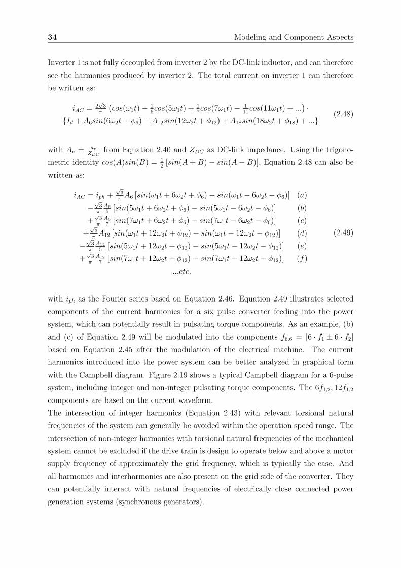
with iph as the Fourier series based on Equation 2.46. Equation 2.49 illustrates selected
components of the current harmonics for a six pulse converter feeding into the power
system, which can potentially result in pulsating torque components. As an example, (b)
and (c) of Equation 2.49 will be modulated into the components f6.6 = |6 · f1 ± 6 · f2|based on Equation 2.45 after the modulation of the electrical machine. The current
harmonics introduced into the power system can be better analyzed in graphical form
with the Campbell diagram. Figure 2.19 shows a typical Campbell diagram for a 6-pulse
system, including integer and non-integer pulsating torque components. The 6f1,2, 12f1,2
components are based on the current waveform.
The intersection of integer harmonics (Equation 2.43) with relevant torsional natural
frequencies of the system can generally be avoided within the operation speed range. The
intersection of non-integer harmonics with torsional natural frequencies of the mechanical
system cannot be excluded if the drive train is design to operate below and above a motor
supply frequency of approximately the grid frequency, which is typically the case. And
all harmonics and interharmonics are also present on the grid side of the converter. They
can potentially interact with natural frequencies of electrically close connected power
generation systems (synchronous generators).

2.3. Power Electronic Devices 35
Figure 2.19: Campbell Diagram of pulsating torque components generated from inter-harmonics and harmonics (Equation 2.49). The two gray lines indicate thecurrent harmonic |6f1 − 5f2| and |6f1 − 7f2|, which are transformed into apulsating torque component of |6f1 − 6f2|.
2.3.2 Self-Commutated Inverter
Self-Commutated Inverters have some significant advantages over line-commutated in-
verter types, as summarized in Table 2.2.
They are known to produce significantly less torque ripple than line-commutated inverters,
which is one critical item for TI in addition to others such as exposure time of excita-
tion and proximity between a generated harmonic and a natural frequency of the drive
train. Self-commutated inverters are still reported as one source of torsional excitation,
e.g. in [28]. Conventional countermeasures to the TI with power electronic devices are
based on increasing the frequency of low order torque harmonics (e.g. by increasing the
converter switching frequency) or by utilizing different control schemes e.g. using Pulse-
Width Modulation (PWM) or hysteresis control instead of square wave. Converter losses
are typically the limitation, which are very critical in high power electronic applications.
The amplitude of low-order torque harmonics can also be reduced by multi-level converter
topologies, where the resulting wave shape is closer to the desired sine wave compared to,
e.g., two level designs. The control complexity as well as the reliability decreases with an
increasing number of devices.
36 Modeling and Component Aspects
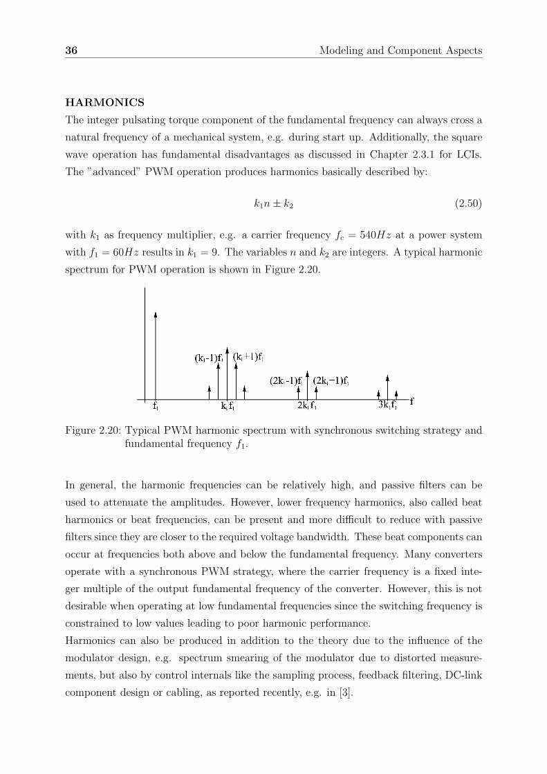
HARMONICS
The integer pulsating torque component of the fundamental frequency can always cross a
natural frequency of a mechanical system, e.g. during start up. Additionally, the square
wave operation has fundamental disadvantages as discussed in Chapter 2.3.1 for LCIs.
The ”advanced” PWM operation produces harmonics basically described by:
k1n ± k2 (2.50)
with k1 as frequency multiplier, e.g. a carrier frequency fc = 540Hz at a power system
with f1 = 60Hz results in k1 = 9. The variables n and k2 are integers. A typical harmonic
spectrum for PWM operation is shown in Figure 2.20.
Figure 2.20: Typical PWM harmonic spectrum with synchronous switching strategy andfundamental frequency f1.
In general, the harmonic frequencies can be relatively high, and passive filters can be
used to attenuate the amplitudes. However, lower frequency harmonics, also called beat
harmonics or beat frequencies, can be present and more difficult to reduce with passive
filters since they are closer to the required voltage bandwidth. These beat components can
occur at frequencies both above and below the fundamental frequency. Many converters
operate with a synchronous PWM strategy, where the carrier frequency is a fixed inte-
ger multiple of the output fundamental frequency of the converter. However, this is not
desirable when operating at low fundamental frequencies since the switching frequency is
constrained to low values leading to poor harmonic performance.
Harmonics can also be produced in addition to the theory due to the influence of the
modulator design, e.g. spectrum smearing of the modulator due to distorted measure-
ments, but also by control internals like the sampling process, feedback filtering, DC-link
component design or cabling, as reported recently, e.g. in [3].
2.4. Summary - Modeling and Component Aspects 37
2.4 Summary - Modeling and Component Aspects
The critical parameter for multi-megawatt drive trains coupled to or electrically close to
power electronic converter is the damping of the mechanical system at its natural fre-
quencies. Low torsional damping parameters (large Q-factors) result into a very sensitive
response to harmonic excitation (Section 2.1.3). Such excitation can easily be caused by
harmonics and interharmonics produced from power conversion units.
A coincidence of electrically generated harmonics with a natural frequency of a large drive
train can result in significant torsional excitation. The most relevant parameter of the
electrical excitation source is its frequency (proximity to critical natural frequencies) and
the exposure time of excitation, not its magnitude. Therefore, a greater electrical excita-
tion source, if not located close to a mechanical resonant frequency, will have less impact
on the shaft than a smaller excitation localized at or near that resonant frequency. None
of the existing converter topologies available for high power applications, voltage source
and current source converter, can generally be excluded from producing harmonics and
interharmonics. Both are potential sources for torsional interaction.


3Torsional Interaction Analysis
Definition of the Torsional Interaction (TI) phenomenon with turbine generators:
”Torsional interaction occurs when the electrically induced subsynchronous torque in the
generator is close to one of the torsional natural modes of the turbine generator shaft.
When this happens, generator rotor oscillations build up and this motion induces armature
voltage components at both subsynchronous and super synchronous frequencies” [29].
3.1 Sources of Excitation for Torsional Oscilla-
tions
Excitation of torsional oscillation always follows the same principle, a disturbance in
the torque-balance between the mechanical system, e.g. compressor load or gas turbine,
and the electrical machine, e.g. motor or generator. These disturbances can be in the
form of step functions but also discrete frequencies, exciting the natural frequency of
the drive train. The magnitude of a resonant vibration depends on the proximity of the
stimulating frequency and a natural frequency, on the magnitude and duration of the
excitation, and on the damping of the excited natural mode [30]. The impact of non-
local ”excitation sources” on large rotational equipment depends on the effective electric
impedance between the source of disturbance and the rotating machinery.
The main disturbances responsible for TI in rotating equipment are grid events [31],
harmonics produced by power conversion, interaction between electrical and mechanical
resonances (subsynchronous resonances which are out of the scope of this thesis) and
improper operation of equipment. TI can lead to increased material fatigue, system
39
40 Torsional Interaction Analysis
outages due to trip, or instantaneous damage of the drive train (see Section 3.2).
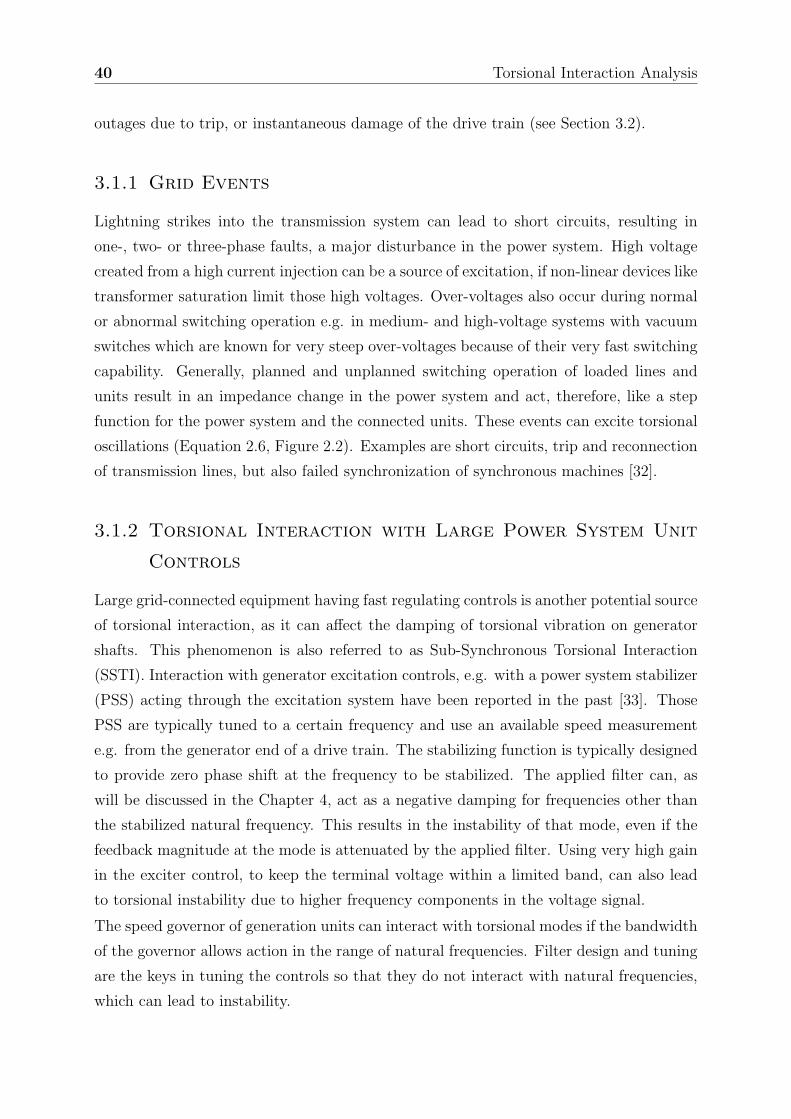
3.1.1 Grid Events
Lightning strikes into the transmission system can lead to short circuits, resulting in
one-, two- or three-phase faults, a major disturbance in the power system. High voltage
created from a high current injection can be a source of excitation, if non-linear devices like
transformer saturation limit those high voltages. Over-voltages also occur during normal
or abnormal switching operation e.g. in medium- and high-voltage systems with vacuum
switches which are known for very steep over-voltages because of their very fast switching
capability. Generally, planned and unplanned switching operation of loaded lines and
units result in an impedance change in the power system and act, therefore, like a step
function for the power system and the connected units. These events can excite torsional
oscillations (Equation 2.6, Figure 2.2). Examples are short circuits, trip and reconnection
of transmission lines, but also failed synchronization of synchronous machines [32].
3.1.2 Torsional Interaction with Large Power System Unit
Controls
Large grid-connected equipment having fast regulating controls is another potential source
of torsional interaction, as it can affect the damping of torsional vibration on generator
shafts. This phenomenon is also referred to as Sub-Synchronous Torsional Interaction
(SSTI). Interaction with generator excitation controls, e.g. with a power system stabilizer
(PSS) acting through the excitation system have been reported in the past [33]. Those
PSS are typically tuned to a certain frequency and use an available speed measurement
e.g. from the generator end of a drive train. The stabilizing function is typically designed
to provide zero phase shift at the frequency to be stabilized. The applied filter can, as
will be discussed in the Chapter 4, act as a negative damping for frequencies other than
the stabilized natural frequency. This results in the instability of that mode, even if the
feedback magnitude at the mode is attenuated by the applied filter. Using very high gain
in the exciter control, to keep the terminal voltage within a limited band, can also lead
to torsional instability due to higher frequency components in the voltage signal.
The speed governor of generation units can interact with torsional modes if the bandwidth
of the governor allows action in the range of natural frequencies. Filter design and tuning
are the keys in tuning the controls so that they do not interact with natural frequencies,
which can lead to instability.

3.1. Sources of Excitation for Torsional Oscillations 41
Power conversion devices, with e.g. constant power control as in HVDC transmission, have
been reported to be a source of torsional excitation: Turbine-generator rotor motion, in
addition to the constant rotational speed, causes variation in both magnitude and phase
angle of the AC-voltage. A line-commutated HVDC system connected and therefore
locked to this AC-voltage modifies the apparent firing angle away from the steady state
phase shift because of equidistant firing angle control. This affects both direct current and
voltage, and thereby the transferred DC-power transferred. The closed loop controls on
direct current, direct voltage or firing angle react to correct for these changes, impacting
magnitude and phase in the DC-transferred power, with the frequency of the initial rotor
motion. The ultimate effect of the change in DC-power is a change in generator air-
gap torque. The impact of the interaction depends on the strength of the AC-system
compared to the DC-system, and on the electric distance between the turbine-generator
and the HVDC system [34], [35].
The Unified Interaction Factor (UIF) [36] has been established as an important design
factor used in preliminary studies to identify potential SSTI based on large-scale interac-
tion studies. The UIF value allows one to decide whether more detailed studies of SSTI
are needed.
3.1.3 Harmonics Produced Due to Power Conversion
Harmonics are produced with all kind of power electronic devices, as already discussed
in Section 2.3. These harmonics are distributed through the connected power system,
dependent on the impedance distribution to connected units like electrical machinery.
They can transform the harmonics with non-fundamental frequency through the air-gap
torque (Section 2.2) and, in case of coincidence of the pulsating torque components with
eigenfrequencies of the mechanical system; they can excite these natural frequencies.
Figure 3.1 represents a Campbell diagram for a 12-pulse LCI, including electrical fre-
quencies (solid), which are mostly dependent on the rotational speed of the drive train;
and mechanical frequencies (dashed) representing the eigenfrequencies of the drive train,
which are typically fixed over the whole operational speed range. The intersection of elec-
trical and mechanical frequencies are called critical speeds; they can result in torsional
interaction, dependent on the amplitude of the pulsating torque (electrical), the mode
shape at this frequency and the effective modal damping.
This effect occurs especially in island-like power systems as shown in Figure 3.2, where
several power electronic loads are connected close to similar sized generation units. In
this case, the magnitude of the harmonics produced can be large enough to significantly
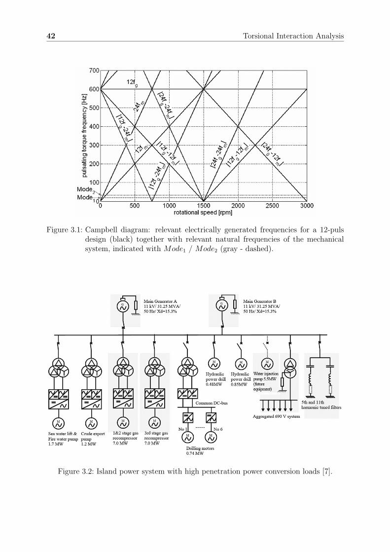
42 Torsional Interaction Analysis
Figure 3.1: Campbell diagram: relevant electrically generated frequencies for a 12-pulsdesign (black) together with relevant natural frequencies of the mechanicalsystem, indicated with Mode1 / Mode2 (gray - dashed).
Figure 3.2: Island power system with high penetration power conversion loads [7].
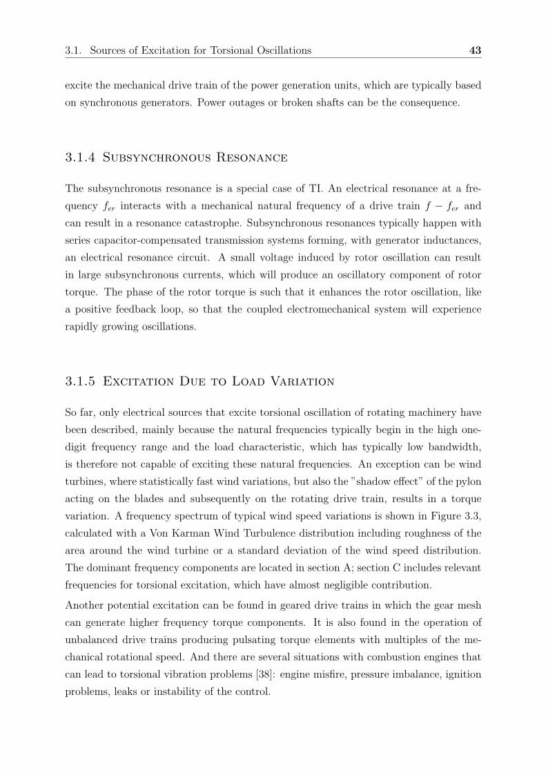
3.1. Sources of Excitation for Torsional Oscillations 43
excite the mechanical drive train of the power generation units, which are typically based
on synchronous generators. Power outages or broken shafts can be the consequence.
3.1.4 Subsynchronous Resonance
The subsynchronous resonance is a special case of TI. An electrical resonance at a fre-
quency fer interacts with a mechanical natural frequency of a drive train f − fer and
can result in a resonance catastrophe. Subsynchronous resonances typically happen with
series capacitor-compensated transmission systems forming, with generator inductances,
an electrical resonance circuit. A small voltage induced by rotor oscillation can result
in large subsynchronous currents, which will produce an oscillatory component of rotor
torque. The phase of the rotor torque is such that it enhances the rotor oscillation, like
a positive feedback loop, so that the coupled electromechanical system will experience
rapidly growing oscillations.
3.1.5 Excitation Due to Load Variation
So far, only electrical sources that excite torsional oscillation of rotating machinery have
been described, mainly because the natural frequencies typically begin in the high one-
digit frequency range and the load characteristic, which has typically low bandwidth,
is therefore not capable of exciting these natural frequencies. An exception can be wind
turbines, where statistically fast wind variations, but also the ”shadow effect” of the pylon
acting on the blades and subsequently on the rotating drive train, results in a torque
variation. A frequency spectrum of typical wind speed variations is shown in Figure 3.3,
calculated with a Von Karman Wind Turbulence distribution including roughness of the
area around the wind turbine or a standard deviation of the wind speed distribution.
The dominant frequency components are located in section A; section C includes relevant
frequencies for torsional excitation, which have almost negligible contribution.
Another potential excitation can be found in geared drive trains in which the gear mesh
can generate higher frequency torque components. It is also found in the operation of
unbalanced drive trains producing pulsating torque elements with multiples of the me-
chanical rotational speed. And there are several situations with combustion engines that
can lead to torsional vibration problems [38]: engine misfire, pressure imbalance, ignition
problems, leaks or instability of the control.
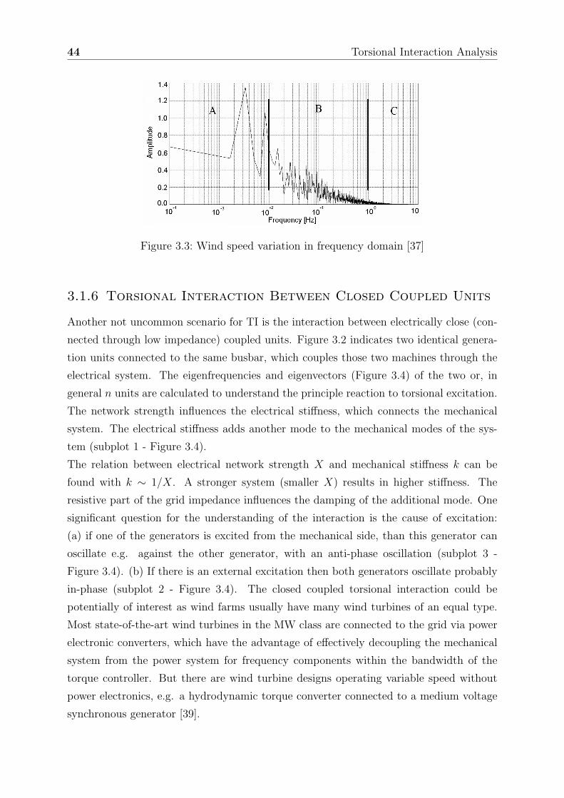
44 Torsional Interaction Analysis
Figure 3.3: Wind speed variation in frequency domain [37]
3.1.6 Torsional Interaction Between Closed Coupled Units
Another not uncommon scenario for TI is the interaction between electrically close (con-
nected through low impedance) coupled units. Figure 3.2 indicates two identical genera-
tion units connected to the same busbar, which couples those two machines through the
electrical system. The eigenfrequencies and eigenvectors (Figure 3.4) of the two or, in
general n units are calculated to understand the principle reaction to torsional excitation.
The network strength influences the electrical stiffness, which connects the mechanical
system. The electrical stiffness adds another mode to the mechanical modes of the sys-
tem (subplot 1 - Figure 3.4).
The relation between electrical network strength X and mechanical stiffness k can be
found with k ∼ 1/X. A stronger system (smaller X) results in higher stiffness. The
resistive part of the grid impedance influences the damping of the additional mode. One
significant question for the understanding of the interaction is the cause of excitation:
(a) if one of the generators is excited from the mechanical side, than this generator can
oscillate e.g. against the other generator, with an anti-phase oscillation (subplot 3 -
Figure 3.4). (b) If there is an external excitation then both generators oscillate probably
in-phase (subplot 2 - Figure 3.4). The closed coupled torsional interaction could be
potentially of interest as wind farms usually have many wind turbines of an equal type.
Most state-of-the-art wind turbines in the MW class are connected to the grid via power
electronic converters, which have the advantage of effectively decoupling the mechanical
system from the power system for frequency components within the bandwidth of the
torque controller. But there are wind turbine designs operating variable speed without
power electronics, e.g. a hydrodynamic torque converter connected to a medium voltage
synchronous generator [39].

3.1. Sources of Excitation for Torsional Oscillations 45
Figure 3.4: Combined mode shape of two (a, b) electrically close coupled units of typeFigure 2.8. Both units have three main masses (1, 2, 3). The original 2nd
natural frequency (subplots(4,5)) is not significantly influenced from the net-work parameter, as there is no strong coupling of this mode to the electricalmachine (distance between mode shape and x-axis for 1a and 1b).
46 Torsional Interaction Analysis
Figure 3.5: Mode frequency dependent on system strength, represented in a power systemequivalent. Mode 1 is the system mode, where both units oscillate against eachother (black).
Figure 3.5 indicates the dependency of the eigenmodes of two electrically close generators
on the electrical coupling between the generators. A low coupling (low stiffness) results in
equal eigenfrequency of the in-phase and anti-phase modes. The difference between the
modes increases with increased stiffness of the electrical coupling of the system.
3.2 Impact of Torsional Interaction
Lifetime reduction is one major impact of TI, as alternating load cycles can have significant
influence on the remaining lifetime of the mechanical system. But there are other factors
to be considered with TI. For instance, expensive equipment is protected against TI, and
may have to be tripped at a certain level of vibration, with the possible consequence of
system outages, as reported in [7].
3.2.1 Lifetime Reduction
A broken turbo generator shaft was the first incident in which the impact of subsyn-
chronous resonances, a kind of TI, was recognized [40]. Broken shafts as a result of TI
represent worst-case lifetime reduction, and can hardly be found in literature. But it is
quite common in industry not to publish severe damages.
The majority of known TI’s impact the lifetime of a system because of the increased stress

3.2. Impact of Torsional Interaction 47
at shaft sections and couplings of rotating machinery. Components usually fail because of
fatigue. Fatigue is defined as failure at relatively low stress levels caused by repeated load
cycling [41]. The alternating torque amplitude, the average value of the cycles and the
number of load cycles, influences the lifetime consumption of mechanical shafts. Typical
alternating torque limits for drive trains in the multi-megawatt range are below 20% to
30% of the static torque rating. Fatigue damage from torsional vibration is cumulative
over many events. TI can frequently induce relatively small torsional vibration in addi-
tion to the static (nominal) torque, so that high generator shaft lifetime expenditure can
quickly be accumulated.
The assessment of the impact is mainly based on empiric knowledge and numerous mate-
rial tests. There are several monitoring systems which estimate the shaft fatigue damage
including loss-of-life per event and cumulative loss-of-life for planning maintenance or in-
spection while damage is minimal, to prevent more costly repairs [42]. Those systems are
only utilized with very expensive generator units in power plants, e.g. with ratings above
100MW .
A common approach in industry to guarantee a certain lifetime with alternating torques
during operation is to over-dimension the shaft to sustain higher alternating torques. But
there are economical limits for over-engineering large rotor shaft systems, especially at
high rated power levels.
3.2.2 Loss of Production
Large generation units with comparably high Q-factor are typically equipped with moni-
toring and protection mechanism, to disconnect the electrical machine as a consequence
of uncontrolled excitation of torsional oscillations, to prevent mechanical damage, such
as failed couplings or broken shafts. Examples for protective devices are torsional motion
relay, armature current relay or unit tripping logic schemes [5].
Protection schemes mainly based on vibration measurements are applied for synchronous
motor driven compressor trains in the multi-megawatt range. They trip the total com-
pression system after certain level of alternating torque is reached (Figure 1.2). The
protection algorithm can be quite complex, as many criteria have to be considered to
prevent unwanted system trips.
3.2.3 Vibration - Noise
Torsional interaction can cause torsional vibration, which can be transferred via a gearbox
into lateral vibrations. These vibrations can potentially cause high sound pressure levels,
48 Torsional Interaction Analysis
which can exceed stringent environmental requirements, e.g. for systems installed in
densely populated areas with low-noise requirements. Problems are known e.g. for wind
turbines, where gear-mesh excitation could potentially excite acoustic resonances resulting
in high noise pressure levels.
3.3 Summary - Torsional Interaction Analysis
The consideration of torsional interaction is important for high power systems, in indus-
trial as well as in power generation applications. Torsional interaction directly affects the
operation of the system only in a minority of cases, e.g. in cases with subsynchronous
resonances, where the system can be damaged within seconds or with system blackouts
due to a protective shut down of generation units.
More frequent are effects that are identified after months or years because of broken shafts
or damaged gearboxes. The reason is mainly the unknown stress in the mechanical shaft
due to torsional interaction because of lack of appropriate sensors connected to the shaft
(Section 5.1). Some industries, like Oil & Gas, require a torsional analysis in the design
phase e.g. for centrifugal compressor systems.
But it is not always possible to prevent excitation of torsional interaction during opera-
tion, especially with growing complexity in industrial power systems due to an increased
percentage of power electronic loads.
4Damping of Torsional Interaction
Effects in Power Systems
Torsional interaction resulting in excitation of torsional oscillation can be observed mainly
in large rotating machinery. Countermeasures have been discussed for decades [43] because
of fatigue and subsequent structural failure of the equipment, but also because of noise
generation (Section 3.2). The focus of this chapter is on damping of torsional oscillations
in large drive trains for industrial or utility applications, since large drive trains have
typically low damping properties and low natural frequencies.
In case of large drive trains with low damping properties, it is impossible to design an
overall system, which operates in all conditions without experiencing any of the discussed
effects at the natural frequency of the drive train. This makes it necessary to apply coun-
termeasures against TI to the system, to prevent fatigue effects and to stay operational
over the specified lifetime of the system.
4.1 State of the Art - Countermeasures against TI
Large drive trains have unique properties compared to other mechanical systems:
1. Low inherent damping, high Q-values, as discussed in previous sections
2. Natural frequencies in the subsynchronous range
3. High initial and operational costs
49
50 Damping of Torsional Interaction Effects in Power Systems
It is very challenging to apply new damping strategies because of the technical properties
mentioned and a conservative operational attitude of the drive train owners. Hence the
existing solutions for active damping in the area of large drive trains are quite limited.
4.1.1 Passive Countermeasures
Passive countermeasures have advantages in reliability terms, but are limited in possi-
ble application, are less flexible and have typically higher initial costs. They have to be
considered in the design process to be applied, retrofit solutions are quire rare. One can
distinguish between mechanical and electrical counter-measures:
A very common countermeasure against TI is to Shift Resonant Frequencies by modi-
fying the drive train stiffness and/or inertia, e.g. by changing the shaft material, diameter
or overall length, mainly during the design phase. This can be done when the expected
frequency spectrum of pulsating torques is known, e.g. with known electrical resonance
frequencies in the power system, which is fixed as long as there are no changes in the
system. [38] reported several cases where adding a flywheel to the main shaft resolved the
problem of torsional interaction, at the expense of changing the mechanical design of the
drive train. This approach works only for relevant harmonics with fixed frequency com-
ponent. Viscous dampers are often used in reciprocating engines to help limit torsional
vibration and crankshaft stresses. A viscous damper consists of a flywheel that rotates
inside the housing, which contains a viscous fluid such as silicon oil that provides a shear
motion of the fluid between the internal flywheel and damper housing. The damping
characteristics can be adjusted by changing the internal clearances between the housing
and flywheel. Adding Soft Couplings with damping components, usually rubber, can
achieve an increase in the overall system damping of a mechanical drive train [38] plus
detuning the torsional natural frequency of the shaft. The coupling is termed ”soft” be-
cause it typically has a lower torsional stiffness than the shafts it is connected to. Soft
couplings are not preferred because of increased maintenance, and they are not available
for drive trains in the multi-megawatt range [41].
Another mechanical approach is a Passive Absorber with inertia Ja, stiffness ka and
damping da, attached to a primary mechanical system. It is tuned to absorb the energy
of an undesired critical frequency with ωc =√
ka/Ja, which cannot fully be achieved
because of the presence of the damping value da. The mechanical properties of a pas-
sive damping device cannot be adjusted, resulting in a very narrow and fixed interval of
operating frequency to be damped. The passive damping device coupled to the original
mechanical design adds another degree of freedom to the primary structure, with an addi-
4.1. State of the Art - Countermeasures against TI 51
tional natural frequency of the overall system. A theoretical elimination of the undesired
critical frequency ωc results therefore in two new natural frequencies, appearing typically
as sidebands of the undesired natural frequency. The distance to the ”old” natural fre-
quency depends on the physical dimensions of the passive damping device. Numerous
variations and improvements to the passive absorber structure can be found in the liter-
ature, e.g. in [44], [45]. They deal with ideal resonators by active elimination of da, but
also with actively tuned absorber devices with superimposed angle dependent reactions
(varying effective ka) or acceleration-dependent reactions (varying effective Ja), for a wide
frequency operation up to damping all frequencies in a certain band. All partially passive
methods need additional components attached to the primary mechanical system, which
is typically undesirable for high power rotational drive trains.
A Static Blocking Filter made up of LC-tank circuits inserted in series with the device
to be protected can be tuned to contribute positive resistance with frequencies, which are
coincident with the complement of the torsional natural frequencies. In essence, the filter
isolates the machine from the system at the critical natural frequency. This hardware is
expensive, and can’t be applied e.g. to power electronics-driven electrical machinery [43].
A similar approach is a Line Filter, which can protect a conventional unit from torsional
interaction when the source of the problem is a single line, but it loses its effectiveness
with changes in the power system.
A Bypass Damping Filter based on a resistor in series with a parallel combination of
a reactor and a capacitor are tuned to have very high impedance at system frequency,
and relatively low impedance at the complement of the torsional natural frequency of the
conventional unit to be protected.
All filters have the drawback that this kind of equipment is limited in flexibility, requires
design changes to the existing power system, and becomes expensive at high voltages
levels.
4.1.2 Active Countermeasures
The active countermeasures can also be divided into mechanical and electrical counter-
measures. The active electrical countermeasures typically try to avoid the coincidence
between complementary electrical and torsional natural frequencies in the system, or
they try to eliminate the complementary electrical frequency components, e.g. by means
of control or a specific switching algorithm for power electronic devices, especially with
voltage source converters. Active mechanical countermeasures improve the mechanical
system at the natural frequency to be less sensitive at those points.
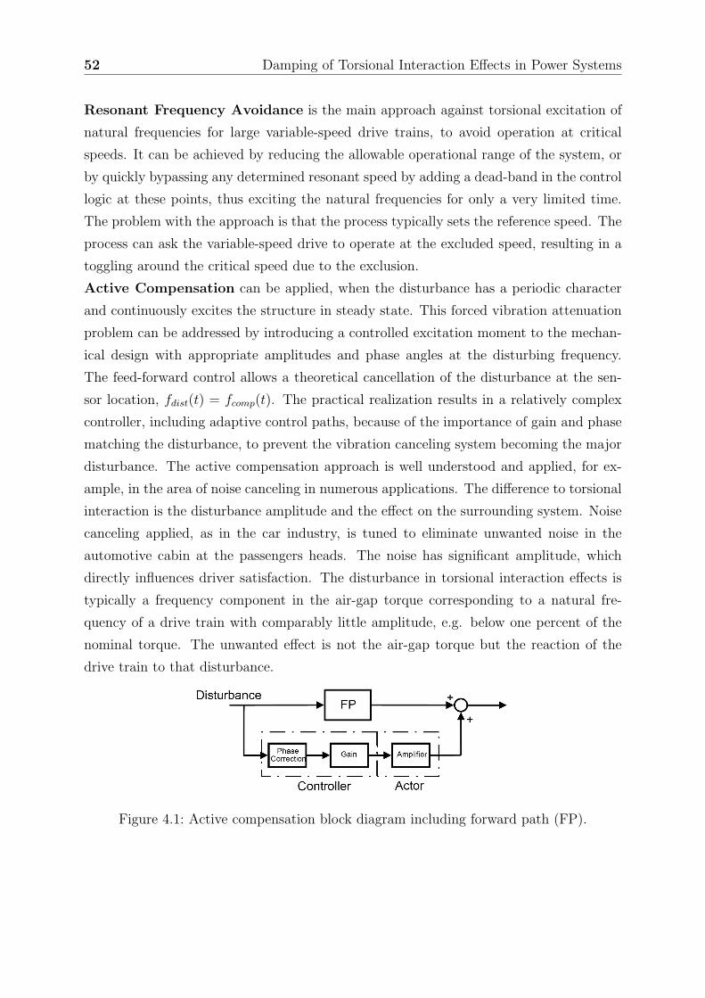
52 Damping of Torsional Interaction Effects in Power Systems
Resonant Frequency Avoidance is the main approach against torsional excitation of
natural frequencies for large variable-speed drive trains, to avoid operation at critical
speeds. It can be achieved by reducing the allowable operational range of the system, or
by quickly bypassing any determined resonant speed by adding a dead-band in the control
logic at these points, thus exciting the natural frequencies for only a very limited time.
The problem with the approach is that the process typically sets the reference speed. The
process can ask the variable-speed drive to operate at the excluded speed, resulting in a
toggling around the critical speed due to the exclusion.
Active Compensation can be applied, when the disturbance has a periodic character
and continuously excites the structure in steady state. This forced vibration attenuation
problem can be addressed by introducing a controlled excitation moment to the mechan-
ical design with appropriate amplitudes and phase angles at the disturbing frequency.
The feed-forward control allows a theoretical cancellation of the disturbance at the sen-
sor location, fdist(t) = fcomp(t). The practical realization results in a relatively complex
controller, including adaptive control paths, because of the importance of gain and phase
matching the disturbance, to prevent the vibration canceling system becoming the major
disturbance. The active compensation approach is well understood and applied, for ex-
ample, in the area of noise canceling in numerous applications. The difference to torsional
interaction is the disturbance amplitude and the effect on the surrounding system. Noise
canceling applied, as in the car industry, is tuned to eliminate unwanted noise in the
automotive cabin at the passengers heads. The noise has significant amplitude, which
directly influences driver satisfaction. The disturbance in torsional interaction effects is
typically a frequency component in the air-gap torque corresponding to a natural fre-
quency of a drive train with comparably little amplitude, e.g. below one percent of the
nominal torque. The unwanted effect is not the air-gap torque but the reaction of the
drive train to that disturbance.
Figure 4.1: Active compensation block diagram including forward path (FP).
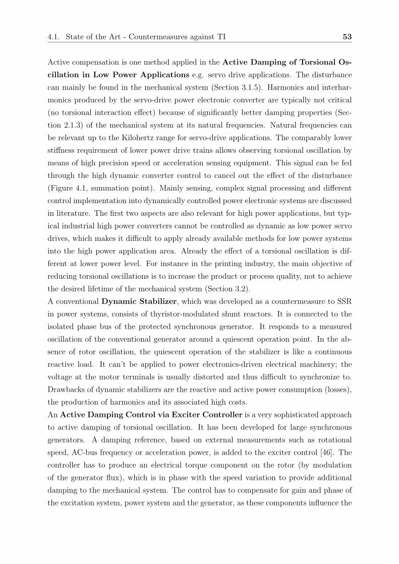
4.1. State of the Art - Countermeasures against TI 53
Active compensation is one method applied in the Active Damping of Torsional Os-
cillation in Low Power Applications e.g. servo drive applications. The disturbance
can mainly be found in the mechanical system (Section 3.1.5). Harmonics and interhar-
monics produced by the servo-drive power electronic converter are typically not critical
(no torsional interaction effect) because of significantly better damping properties (Sec-
tion 2.1.3) of the mechanical system at its natural frequencies. Natural frequencies can
be relevant up to the Kilohertz range for servo-drive applications. The comparably lower
stiffness requirement of lower power drive trains allows observing torsional oscillation by
means of high precision speed or acceleration sensing equipment. This signal can be fed
through the high dynamic converter control to cancel out the effect of the disturbance
(Figure 4.1, summation point). Mainly sensing, complex signal processing and different
control implementation into dynamically controlled power electronic systems are discussed
in literature. The first two aspects are also relevant for high power applications, but typ-
ical industrial high power converters cannot be controlled as dynamic as low power servo
drives, which makes it difficult to apply already available methods for low power systems
into the high power application area. Already the effect of a torsional oscillation is dif-
ferent at lower power level. For instance in the printing industry, the main objective of
reducing torsional oscillations is to increase the product or process quality, not to achieve
the desired lifetime of the mechanical system (Section 3.2).
A conventional Dynamic Stabilizer, which was developed as a countermeasure to SSR
in power systems, consists of thyristor-modulated shunt reactors. It is connected to the
isolated phase bus of the protected synchronous generator. It responds to a measured
oscillation of the conventional generator around a quiescent operation point. In the ab-
sence of rotor oscillation, the quiescent operation of the stabilizer is like a continuous
reactive load. It can’t be applied to power electronics-driven electrical machinery; the
voltage at the motor terminals is usually distorted and thus difficult to synchronize to.
Drawbacks of dynamic stabilizers are the reactive and active power consumption (losses),
the production of harmonics and its associated high costs.
An Active Damping Control via Exciter Controller is a very sophisticated approach
to active damping of torsional oscillation. It has been developed for large synchronous
generators. A damping reference, based on external measurements such as rotational
speed, AC-bus frequency or acceleration power, is added to the exciter control [46]. The
controller has to produce an electrical torque component on the rotor (by modulation
of the generator flux), which is in phase with the speed variation to provide additional
damping to the mechanical system. The control has to compensate for gain and phase of
the excitation system, power system and the generator, as these components influence the

54 Damping of Torsional Interaction Effects in Power Systems
effect of the generator flux on the resulting torque [47]. The typical frequencies of applica-
tion are in the range of approximately 0.2Hz to 2.5Hz, sufficient for very large generation
units. Higher natural frequencies can hardly be addressed because of time constraints of
the exciter converter and the exciter implementation, especially for rotating exciter.
4.2 New Damping Approach
None of the available approaches (Section 4.1) is capable of enabling electrically driven
multi-megawatt trains and power generation units to operate in their designed way with-
out being possibly affected by torsional interactions. Large drive trains have very limited
damping properties (Section 2.1.3). This makes them very sensitive to torsional interac-
tion. The approach introduced and developed within this section decreases the inherent
sensitivity of the mechanical system and thus allows operation of such multi-megawatt
drive trains without the negative effects discussed in Section 3.2.
The damping method chosen for application with large drive trains can be derived from
Newton’s equation of motion:
[J] ·
φ
+ [D] ·
φ
+ [K] · φ = [B] · u (4.1)
where J represents the systems matrix of inertia, D the damping matrix and K the stiff-
ness matrix. The part of the equation to the left of the equal sign describes the mechanical
system with its properties, as described in the Chapter 2. The matrix B, on the right side
of the equation, represents all input components acting on the mechanical system, includ-
ing pulsating torque components. The basic approach of the developed active damping
method is to modify B in such a way that it behaves like an increased damping matrix
D on the mechanical system, but only at the natural frequencies of the system, where an
increased damping is required. This is achieved by basically modulating active power at
the natural frequency of the sensitive drive train.
The developed method is a mechatronic control approach. It utilizes a mechanical feed-
back signal to introduce limited damping power, and it has the capability to compensate
for dead times typically existing in large converters without significant loss of damping
performance. It provides a very robust design for slight natural frequency variation and
mistuning although it modulates active power exactly at the resonant frequencies of the
mechanical system. It operates only at the natural frequency of the sensitive drive train,
and allows high damping performance with very limited power. More than one mode
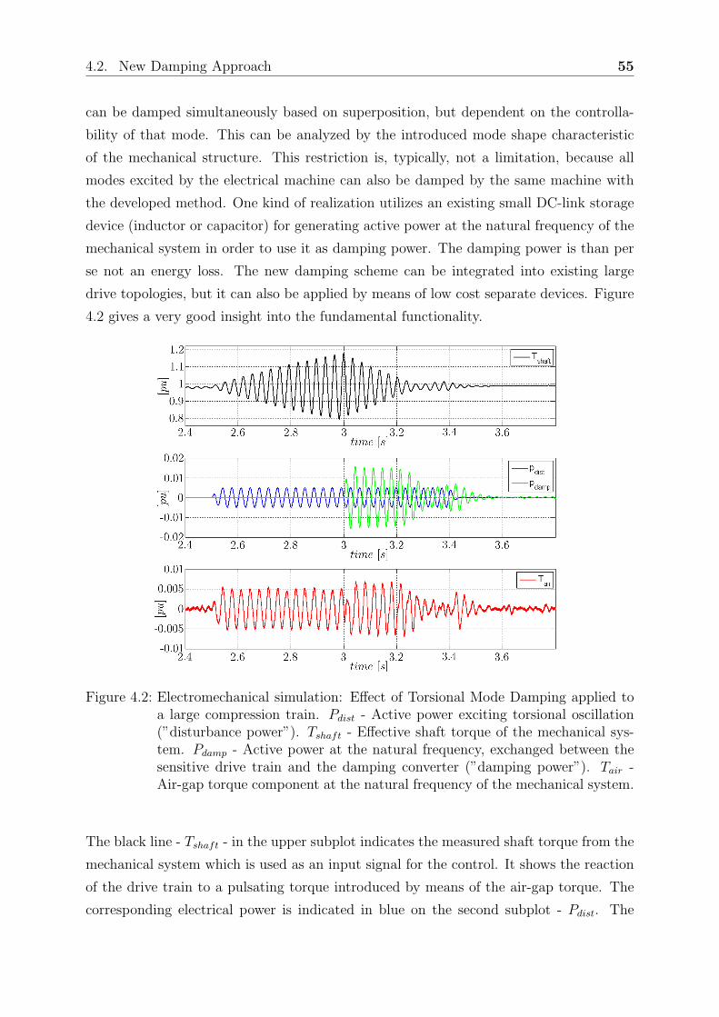
4.2. New Damping Approach 55
can be damped simultaneously based on superposition, but dependent on the controlla-
bility of that mode. This can be analyzed by the introduced mode shape characteristic
of the mechanical structure. This restriction is, typically, not a limitation, because all
modes excited by the electrical machine can also be damped by the same machine with
the developed method. One kind of realization utilizes an existing small DC-link storage
device (inductor or capacitor) for generating active power at the natural frequency of the
mechanical system in order to use it as damping power. The damping power is than per
se not an energy loss. The new damping scheme can be integrated into existing large
drive topologies, but it can also be applied by means of low cost separate devices. Figure
4.2 gives a very good insight into the fundamental functionality.
Figure 4.2: Electromechanical simulation: Effect of Torsional Mode Damping applied toa large compression train. Pdist - Active power exciting torsional oscillation(”disturbance power”). Tshaft - Effective shaft torque of the mechanical sys-tem. Pdamp - Active power at the natural frequency, exchanged between thesensitive drive train and the damping converter (”damping power”). Tair -Air-gap torque component at the natural frequency of the mechanical system.
The black line - Tshaft - in the upper subplot indicates the measured shaft torque from the
mechanical system which is used as an input signal for the control. It shows the reaction
of the drive train to a pulsating torque introduced by means of the air-gap torque. The
corresponding electrical power is indicated in blue on the second subplot - Pdist. The
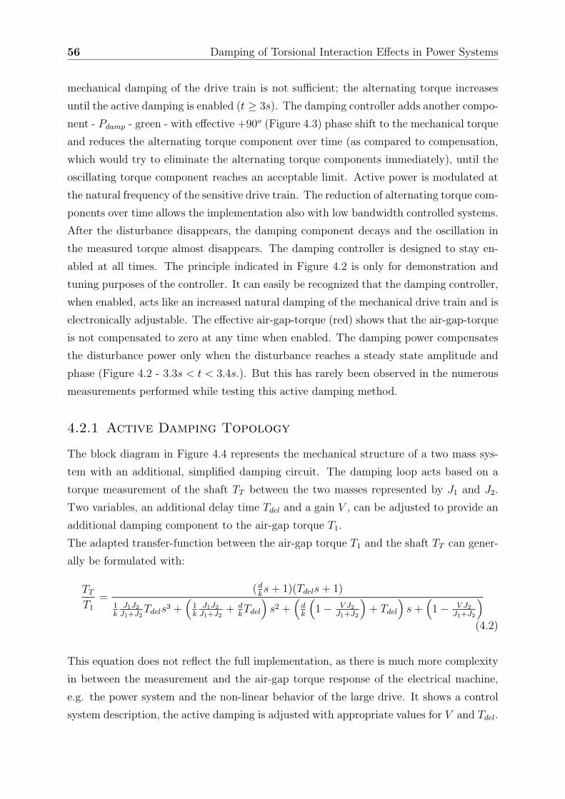
56 Damping of Torsional Interaction Effects in Power Systems
mechanical damping of the drive train is not sufficient; the alternating torque increases
until the active damping is enabled (t ≥ 3s). The damping controller adds another compo-
nent - Pdamp - green - with effective +90o (Figure 4.3) phase shift to the mechanical torque
and reduces the alternating torque component over time (as compared to compensation,
which would try to eliminate the alternating torque components immediately), until the
oscillating torque component reaches an acceptable limit. Active power is modulated at
the natural frequency of the sensitive drive train. The reduction of alternating torque com-
ponents over time allows the implementation also with low bandwidth controlled systems.
After the disturbance disappears, the damping component decays and the oscillation in
the measured torque almost disappears. The damping controller is designed to stay en-
abled at all times. The principle indicated in Figure 4.2 is only for demonstration and
tuning purposes of the controller. It can easily be recognized that the damping controller,
when enabled, acts like an increased natural damping of the mechanical drive train and is
electronically adjustable. The effective air-gap-torque (red) shows that the air-gap-torque
is not compensated to zero at any time when enabled. The damping power compensates
the disturbance power only when the disturbance reaches a steady state amplitude and
phase (Figure 4.2 - 3.3s < t < 3.4s.). But this has rarely been observed in the numerous
measurements performed while testing this active damping method.
4.2.1 Active Damping Topology
The block diagram in Figure 4.4 represents the mechanical structure of a two mass sys-
tem with an additional, simplified damping circuit. The damping loop acts based on a
torque measurement of the shaft TT between the two masses represented by J1 and J2.
Two variables, an additional delay time Tdel and a gain V , can be adjusted to provide an
additional damping component to the air-gap torque T1.
The adapted transfer-function between the air-gap torque T1 and the shaft TT can gener-
ally be formulated with:
TT
T1
=( d
ks + 1)(Tdels + 1)
1k
J1J2
J1+J2Tdels3 +
(
1k
J1J2
J1+J2+ d
kTdel
)
s2 +(
dk
(
1 − V J2
J1+J2
)
+ Tdel
)
s +(
1 − V J2
J1+J2
)
(4.2)
This equation does not reflect the full implementation, as there is much more complexity
in between the measurement and the air-gap torque response of the electrical machine,
e.g. the power system and the non-linear behavior of the large drive. It shows a control
system description, the active damping is adjusted with appropriate values for V and Tdel.
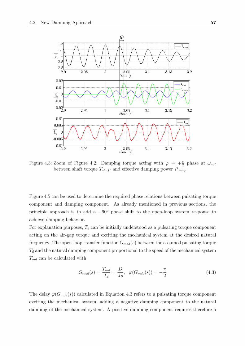
4.2. New Damping Approach 57
Figure 4.3: Zoom of Figure 4.2: Damping torque acting with ϕ = +π2
phase at ωnat
between shaft torque Tshaft and effective damping power Pdamp.
Figure 4.5 can be used to determine the required phase relations between pulsating torque
component and damping component. As already mentioned in previous sections, the
principle approach is to add a +90o phase shift to the open-loop system response to
achieve damping behavior.
For explanation purposes, Td can be initially understood as a pulsating torque component
acting on the air-gap torque and exciting the mechanical system at the desired natural
frequency. The open-loop transfer-function Gmdd(s) between the assumed pulsating torque
Td and the natural damping component proportional to the speed of the mechanical system
Tmd can be calculated with:
Gmdd(s) =Tmd
Td
=D
Js, ϕ(Gmdd(s)) = −π
2(4.3)
The delay ϕ(Gmdd(s)) calculated in Equation 4.3 refers to a pulsating torque component
exciting the mechanical system, adding a negative damping component to the natural
damping of the mechanical system. A positive damping component requires therefore a

58 Damping of Torsional Interaction Effects in Power Systems
Figure 4.4: Mechanical model representation with theoretical active damping loop
Figure 4.5: Active damping component Td acting through the air-gap torque on the me-chanical system.
phase shift between the introduced pulsating damping torque and the natural damping
of:
ϕ(Gmdd(s))!= +
π
2(4.4)
These relations can also be observed in the demonstration plot (Figure 4.3). The single
sine periodicity of the oscillating torque component allows the utilization of the damping
structure also with topologies including delay or dead-time behavior; the positive damping
torque can also be achieved with a delay of:
ϕ(Gmdd(s))!=
π
2+ n · 2π (4.5)
with n = 0, 1, 2, .... The influence of the delayed damping on the damping performance
depends mainly on the natural damping of the mechanical system, and can be almost
neglected for large systems because of their low natural damping. When applying a
delayed damping power, it is not possible to completely eliminate torsional oscillations.

4.2. New Damping Approach 59
But this is not needed in high power drive trains where small torsional oscillations are
well within the specification limits.
4.2.2 Implementation of the Active Damping Method
Two main designs have been identified to be suitable as a platform for the implementation
of the damping structure:
• Integrated into a power conversion system utilizing the available hardware to provide
damping to the variable speed driven electrical machine, on the machine side of the
converter.
• Integrated into a power conversion system, but acting on the grid side of the con-
verter. This implementation requires care that it does not impact the connected
variable speed drive train by the damping power modulated with the grid.
• A separate power conversion device dedicated to generate active damping power, to
produce air-gap torque harmonics acting as increased natural damping.
More details to the hardware implementation aspects will be given in Chapter 5. The
implementation of the damping structure itself can be divided into three parts:
1. Measurement in the mechanical system providing an analog input signal (”In”)
2. Data processing
3. Analog output and interface to converter control (”Out”)
Figure 4.6: Block diagram of the principle damping circuit implementation, e.g. for damp-ing of two natural frequencies.
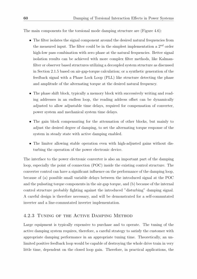
60 Damping of Torsional Interaction Effects in Power Systems
The main components for the torsional mode damping structure are (Figure 4.6):
• The filter isolates the signal component around the desired natural frequencies from
the measured input. The filter could be in the simplest implementation a 2nd order
high-low pass combination with zero phase at the natural frequencies. Better signal
isolation results can be achieved with more complex filter methods, like Kalman-
filter or observer based structures utilizing a decoupled system structure as discussed
in Section 2.1.5 based on air-gap-torque calculation; or a synthetic generation of the
feedback signal with a Phase Lock Loop (PLL) like structure detecting the phase
and amplitude of the alternating torque at the desired natural frequency.
• The phase shift block, typically a memory block with successively writing and read-
ing addresses in an endless loop, the reading address offset can be dynamically
adjusted to allow adjustable time delays, required for compensation of converter,
power system and mechanical system time delays.
• The gain block compensating for the attenuation of other blocks, but mainly to
adjust the desired degree of damping, to set the alternating torque response of the
system in steady state with active damping enabled.
• The limiter allowing stable operation even with high-adjusted gains without dis-
turbing the operation of the power electronic device.
The interface to the power electronic converter is also an important part of the damping
loop, especially the point of connection (POC) inside the existing control structure. The
converter control can have a significant influence on the performance of the damping loop,
because of (a) possible small variable delays between the introduced signal at the POC
and the pulsating torque components in the air-gap torque, and (b) because of the internal
control structure probably fighting against the introduced ”disturbing” damping signal.
A careful design is therefore necessary, and will be demonstrated for a self-commutated
inverter and a line-commutated inverter implementation.
4.2.3 Tuning of the Active Damping Method
Large equipment is typically expensive to purchase and to operate. The tuning of the
active damping system requires, therefore, a careful strategy to satisfy the customer with
appropriate damping performance in an appropriate tuning time. Theoretically, an un-
limited positive feedback loop would be capable of destroying the whole drive train in very
little time, dependent on the closed loop gain. Therefore, in practical applications, the
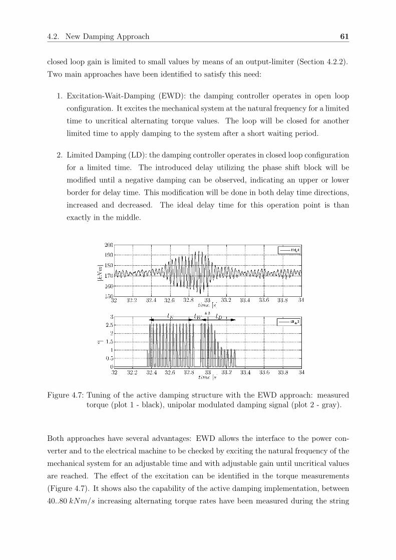
4.2. New Damping Approach 61
closed loop gain is limited to small values by means of an output-limiter (Section 4.2.2).
Two main approaches have been identified to satisfy this need:
1. Excitation-Wait-Damping (EWD): the damping controller operates in open loop
configuration. It excites the mechanical system at the natural frequency for a limited
time to uncritical alternating torque values. The loop will be closed for another
limited time to apply damping to the system after a short waiting period.
2. Limited Damping (LD): the damping controller operates in closed loop configuration
for a limited time. The introduced delay utilizing the phase shift block will be
modified until a negative damping can be observed, indicating an upper or lower
border for delay time. This modification will be done in both delay time directions,
increased and decreased. The ideal delay time for this operation point is than
exactly in the middle.
Figure 4.7: Tuning of the active damping structure with the EWD approach: measuredtorque (plot 1 - black), unipolar modulated damping signal (plot 2 - gray).
Both approaches have several advantages: EWD allows the interface to the power con-
verter and to the electrical machine to be checked by exciting the natural frequency of the
mechanical system for an adjustable time and with adjustable gain until uncritical values
are reached. The effect of the excitation can be identified in the torque measurements
(Figure 4.7). It shows also the capability of the active damping implementation, between
40..80 kNm/s increasing alternating torque rates have been measured during the string
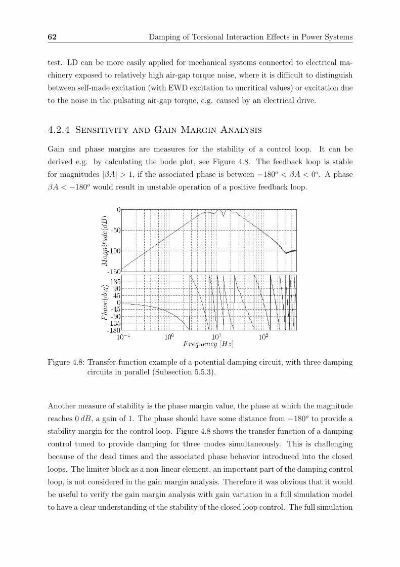
62 Damping of Torsional Interaction Effects in Power Systems
test. LD can be more easily applied for mechanical systems connected to electrical ma-
chinery exposed to relatively high air-gap torque noise, where it is difficult to distinguish
between self-made excitation (with EWD excitation to uncritical values) or excitation due
to the noise in the pulsating air-gap torque, e.g. caused by an electrical drive.
4.2.4 Sensitivity and Gain Margin Analysis
Gain and phase margins are measures for the stability of a control loop. It can be
derived e.g. by calculating the bode plot, see Figure 4.8. The feedback loop is stable
for magnitudes |βA| > 1, if the associated phase is between −180o < βA < 0o. A phase
βA < −180o would result in unstable operation of a positive feedback loop.
Figure 4.8: Transfer-function example of a potential damping circuit, with three dampingcircuits in parallel (Subsection 5.5.3).
Another measure of stability is the phase margin value, the phase at which the magnitude
reaches 0 dB, a gain of 1. The phase should have some distance from −180o to provide a
stability margin for the control loop. Figure 4.8 shows the transfer function of a damping
control tuned to provide damping for three modes simultaneously. This is challenging
because of the dead times and the associated phase behavior introduced into the closed
loops. The limiter block as a non-linear element, an important part of the damping control
loop, is not considered in the gain margin analysis. Therefore it was obvious that it would
be useful to verify the gain margin analysis with gain variation in a full simulation model
to have a clear understanding of the stability of the closed loop control. The full simulation
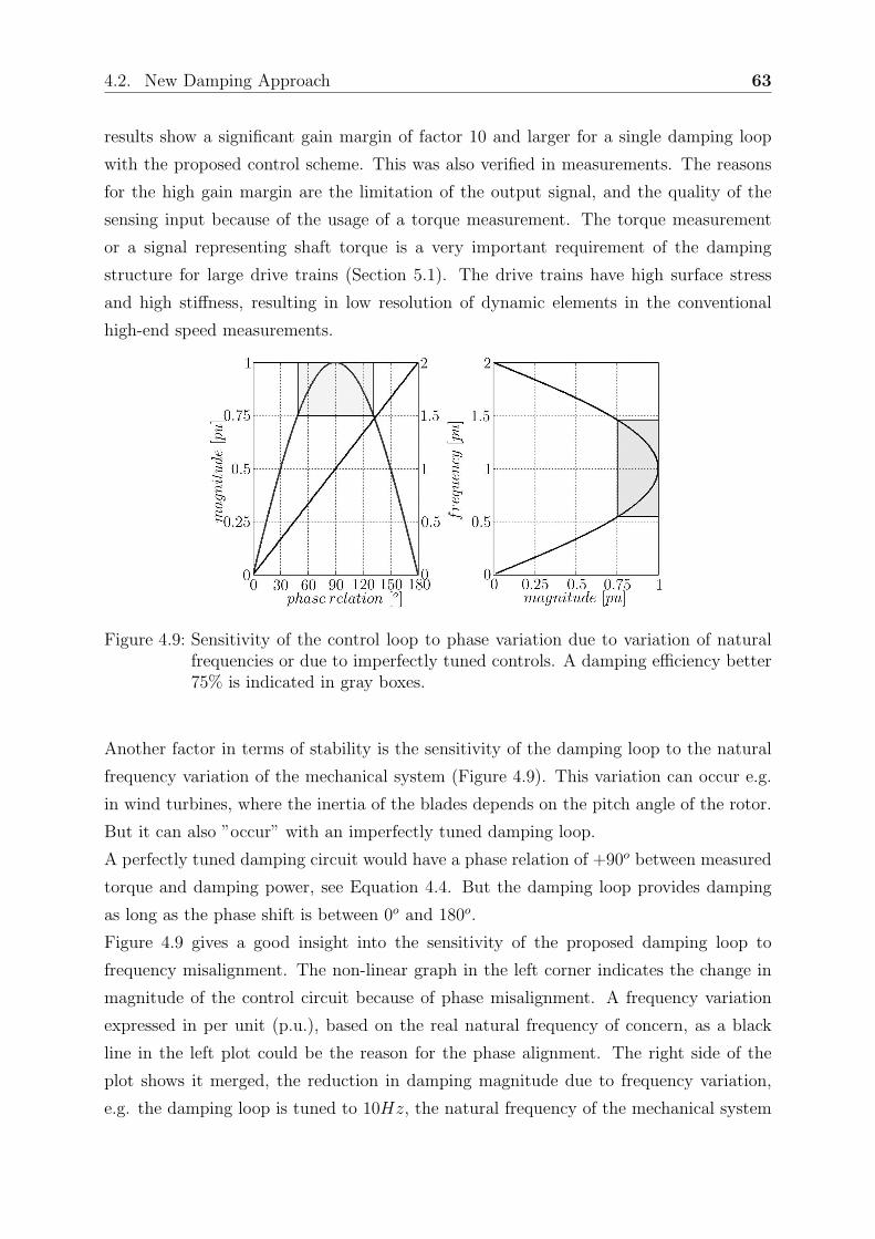
4.2. New Damping Approach 63
results show a significant gain margin of factor 10 and larger for a single damping loop
with the proposed control scheme. This was also verified in measurements. The reasons
for the high gain margin are the limitation of the output signal, and the quality of the
sensing input because of the usage of a torque measurement. The torque measurement
or a signal representing shaft torque is a very important requirement of the damping
structure for large drive trains (Section 5.1). The drive trains have high surface stress
and high stiffness, resulting in low resolution of dynamic elements in the conventional
high-end speed measurements.
Figure 4.9: Sensitivity of the control loop to phase variation due to variation of naturalfrequencies or due to imperfectly tuned controls. A damping efficiency better75% is indicated in gray boxes.
Another factor in terms of stability is the sensitivity of the damping loop to the natural
frequency variation of the mechanical system (Figure 4.9). This variation can occur e.g.
in wind turbines, where the inertia of the blades depends on the pitch angle of the rotor.
But it can also ”occur” with an imperfectly tuned damping loop.
A perfectly tuned damping circuit would have a phase relation of +90o between measured
torque and damping power, see Equation 4.4. But the damping loop provides damping
as long as the phase shift is between 0o and 180o.
Figure 4.9 gives a good insight into the sensitivity of the proposed damping loop to
frequency misalignment. The non-linear graph in the left corner indicates the change in
magnitude of the control circuit because of phase misalignment. A frequency variation
expressed in per unit (p.u.), based on the real natural frequency of concern, as a black
line in the left plot could be the reason for the phase alignment. The right side of the
plot shows it merged, the reduction in damping magnitude due to frequency variation,
e.g. the damping loop is tuned to 10Hz, the natural frequency of the mechanical system
64 Damping of Torsional Interaction Effects in Power Systems
11Hz (1.1p.u.), effecting the damping gain with 0.988p.u., a negligible gain reduction of
1.2%. The damping loop would be unstable for frequencies with fnat ≥ 2 · ftun. Although
the control system has low sensitivity to parameter changes, the mechanical system is
very sensitive to the frequency of the modulated power (system with high amplification
factor Q, see Figure 2.6). The mechanical sensitivity is critical for a synthetic calculated
signal representing the shaft torque, e.g. by utilizing imperfectly tuned observer models,
and uncritical when acting based on a direct measurement from the mechanical system.
4.3 Summary - Damping of Torsional Interaction
Effects in Power Systems
Several approaches as state of the art countermeasures against torsional interaction have
been discussed within this chapter. Most of the passive countermeasures can only be
applied where fixed harmonics cause torsional oscillations, not for variable speed opera-
tion, and are typically difficult to be applied in high power drive trains. The discussed
active countermeasures can usually be found for different power levels: dynamic stabilizer
and exciter control modification in very large generation units, with significantly lower
bandwidth and higher costs due to required modification in the electrical system. Active
compensation as well as other complex control approaches are typically available for low
power applications in the kW range and usually require a sufficient dynamic control and
corresponding power electronic hardware, which is not applied to industrial high power
drive systems.
A new method to increase the damping property of mechanical systems has been intro-
duced in this chapter. It utilizes power electronic devices to exchange active power at the
measured and isolated natural frequency of a drive train with sensitivity to torsional ex-
citations. The method is implemented in such a way that the mechanical system behaves
like with an increased mechanical damping. The damping property is thus electronically
adjustable by modifying control loop settings. The principle implementation of the devel-
oped damping loop is illustrated, and the relevant blocks are discussed. Tuning approaches
are introduced, which are very important for the implementation into real systems. The
proposed damping circuit operates with a measured natural frequency of the mechanical
system but without risks for the mechanical system because the applied damping power
is always limited to small values, by means of a limiter at the interface to the converter
control. The developed method has shown very low sensitivity to parameter changes and
provides a very high gain margin, larger than 10 was verified in field measurements.

5Fields of Application for the Active
Damping Approach
The active damping system acts as an increased natural damping for the mechanical drive
train, and can be applied in different ways. A power electronic device is always needed to
modulate active power through the winding of an electrical machine. There are in general
two options:
1. There is no power electronic device available electrically close to the drive train that
includes an electrical machine.
2. There is already a power electronic device available, which can be used for the
modulation of active power. The requirements for this power electronic device will
be discussed in the second part of this chapter.
The potential hardware implementation with two independent options is indicated in
Figure 5.1. The sensors measuring the mechanical torque of the desired drive train are
located based on the mode shapes of the drive train, and are connected to the ”TMD” box
including, among others, the damping circuit (Figure 4.6). Only one out of two indicated
solutions is needed to provide additional damping to the conventional generation units:
(1) the separate device controlled with the gray line or (2) the integrated solution, utiliz-
ing available converter(s), indicated with numbered dots. There is only a single separate
unit shown, but two potential converters for integrating the damping functionality into
existing units, marked with numbered dots. The number of required units depends on
the necessary damping power level (which is typically less than 1% of the nominal power)
65

66 Fields of Application for the Active Damping Approach
and on the redundancy requirements for the damping solution. Both damping options
will be discussed in this section.
Figure 5.1: Island power system (introduced in Section 3), equipped with a torsional modedamping option to increase the damping properties of both generator drivetrains. One of the available power converters (1) or (2), or a separate dampingconverter can be utilized for this purpose.
The availability of a power electronic system for an active damping implementation de-
pends on (a) the feasibility and effort for modifying this system, (b) the hourly availability,
and also (c) the reliability of the desired active damping solution. The electrically close
requirement implies low impedance between the damping device and the mechanical drive
train compared to the other impedances connected to the same node, to conduct most of
the modulated active power to the desired mechanical system. A weak grid connection
results in relatively high impedance values, one reason why the active damping solution
is perfectly suited for island like power system structures.
Reliability is an important aspect in the active damping approach. Relying on an actively
damping system that is unavailable can lead to severe outages (see Section 3.2). Being
able to observe the availability of the active damping device could be a requirement. Dif-
ferent levels of reliability can be imagined: A watch dog controlling the availability of the
damping control; or a redundant measurement detecting the vibration of the mechanical
system, can set an alarm with abnormal values. A stronger reliability requirement might

5.1. Monitoring of Torsional Oscillations 67
be necessary: a redundant damping solution. A n−1 reliability requires at least n devices
online to provide active damping on demand. The effort for the implementation into ex-
isting systems then depends on the availability of suitable designs. The separate device
(Chapter 5.2) solution can be built relatively easily as a redundant design.
5.1 Monitoring of Torsional Oscillations
Sensing of a torsional oscillation is a critical requirement for the implementation of the
developed damping method. Standard equipment used for analyzing lateral vibrations,
such as accelerometers and proximity probes, are not able to measure torsional vibrations.
Depending on the shape of the torsional mode and the stiffness of the motor coupling,
even high-resolution motor speed measurements may not be able to accurately measure
such vibrations, also due to the comparably small torsion angle at a certain level of
alternating torque. In string tests, torsional oscillation measurements are typically based
on measuring the shaft torque, e.g., by a full-bridge strain gage system with telemetry. If
the shaft torque has to be monitored over long time periods or if the torque signal is used
in a control system, long-term stable measurement methods have to be applied.
Examples for suitable sensing systems are continuous duty (CD) torque-meters for per-
manent installation, which are offered by a variety of vendors. The most widespread CD
sensing technology is based on measuring the twist over a coupling spool, and there are
more than 800 installations worldwide using this approach with many millions of operating
hours accumulated.
To achieve absolute accuracy of the torque measurement in the order of one percent full
scale, such torque-meters must be integrated into the mechanical system design, typically
during the design stage. Therefore it can be costly to apply this type of torque-meter as
a retrofit.
However, for torsional mode damping applications, an absolute accuracy of one percent
full scale is not needed. The most important measured signals in this type of feedback
control system are the frequency and phase of a measured oscillation. An accuracy of ∼ 5%
is sufficient for torsional mode damping, based on own experience. Therefore, alternative
non-contact sensing methods with high long-term stability may be more attractive. As
an example, toothed-wheel based monitoring systems sensing the speed on both ends
of a drive train have a long history of measuring torsional vibrations continuously on
utility-class generating machines.
Proper transduction of the pulses from the sensors, plus knowledge of the torsional mode
shapes, is adequate for detecting torsional vibrations sufficient for both protection and

68 Fields of Application for the Active Damping Approach
damping [48]. This type of sensing and monitoring system has been used in several
dozens of applications with synchronous generators over the last 30 years. Recently, in
another power system application, a magnetostrictive torque sensing system was installed
to monitor the shaft torque at the couplings of two large flywheel generators [49]. The
absolute accuracy of the torque sensors in this application is only in the lower percent
range, but still suited for retrofit applications because it does not require attachment to
the rotating shaft or modification of the existing train.
It is an ongoing effort to improve existing torsional vibration sensor systems with both,
improved sensing devices, but also with model based approaches to better detect the
phase and amplitude of the torsional oscillation.
5.2 Separate Active Damping Device
A separate active damping device can be utilized when there are no or no suitable existing
power electronic devices available electrically close to the mechanical system. Many dif-
ferent design options are feasible for exchanging active power at the natural frequency of
the mechanical drive train between the mechanical system and the separate device. The
separate device always consists of three parts: a separate power conversion module, a load
and a control system including the damping control structure. The vibration sensing in
the mechanical system is assumed to be solved.
A general overview about power electronic converter has already been given in Section
2.3. Both designs (self- and line-commutated converter types) are principally applicable,
dependent on rating, dynamic performance or reliability requirements. Only one conver-
sion from AC to DC is typically necessary to be able to modulate the desired active power
as needed for the active damping (Figure 4.2).
Figure 5.2: Design options for the separate active damping device. Options a and b in-dicate line-commutated converter types, option c and d self commutated con-verter types.
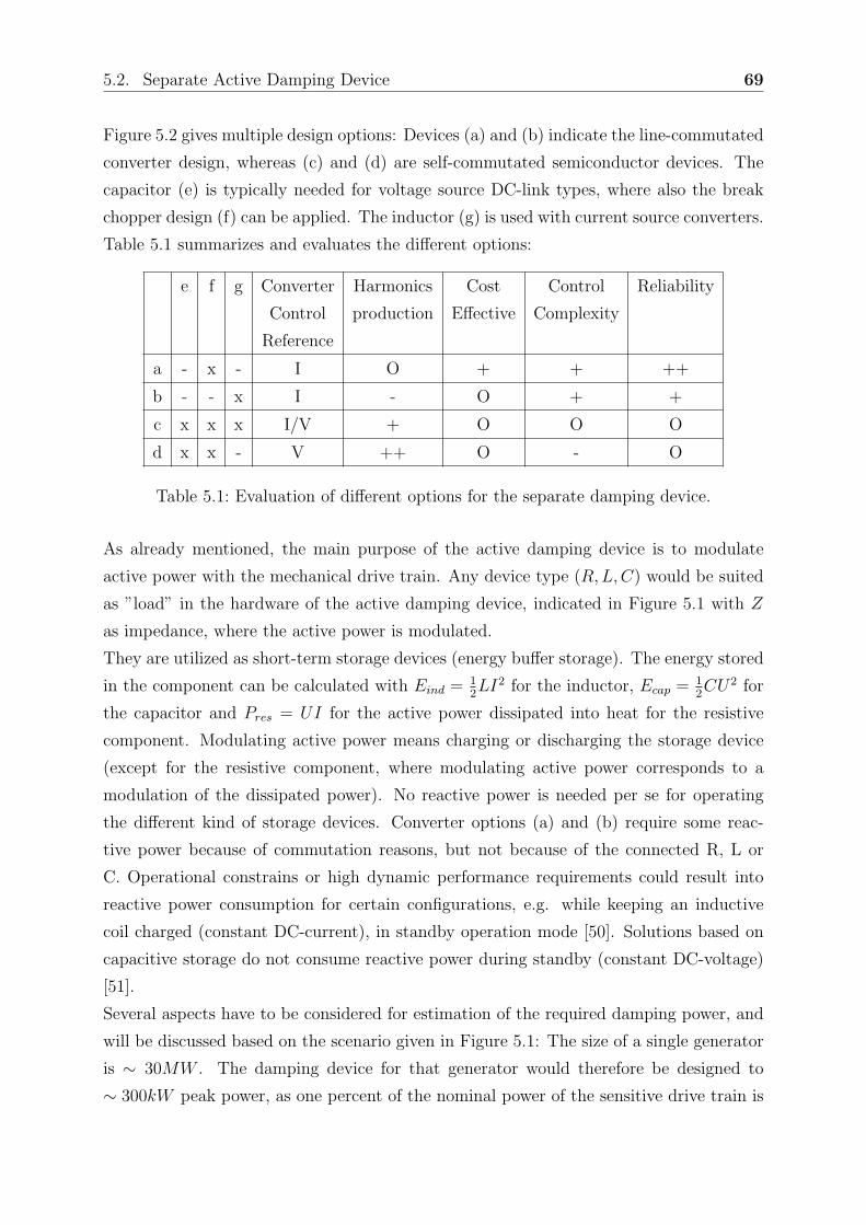
5.2. Separate Active Damping Device 69
Figure 5.2 gives multiple design options: Devices (a) and (b) indicate the line-commutated
converter design, whereas (c) and (d) are self-commutated semiconductor devices. The
capacitor (e) is typically needed for voltage source DC-link types, where also the break
chopper design (f) can be applied. The inductor (g) is used with current source converters.
Table 5.1 summarizes and evaluates the different options:
e f g Converter Harmonics Cost Control Reliability
Control production Effective Complexity
Reference
a - x - I O + + ++
b - - x I - O + +
c x x x I/V + O O O
d x x - V ++ O - O
Table 5.1: Evaluation of different options for the separate damping device.
As already mentioned, the main purpose of the active damping device is to modulate
active power with the mechanical drive train. Any device type (R,L,C) would be suited
as ”load” in the hardware of the active damping device, indicated in Figure 5.1 with Z
as impedance, where the active power is modulated.
They are utilized as short-term storage devices (energy buffer storage). The energy stored
in the component can be calculated with Eind = 12LI2 for the inductor, Ecap = 1
2CU2 for
the capacitor and Pres = UI for the active power dissipated into heat for the resistive
component. Modulating active power means charging or discharging the storage device
(except for the resistive component, where modulating active power corresponds to a
modulation of the dissipated power). No reactive power is needed per se for operating
the different kind of storage devices. Converter options (a) and (b) require some reac-
tive power because of commutation reasons, but not because of the connected R, L or
C. Operational constrains or high dynamic performance requirements could result into
reactive power consumption for certain configurations, e.g. while keeping an inductive
coil charged (constant DC-current), in standby operation mode [50]. Solutions based on
capacitive storage do not consume reactive power during standby (constant DC-voltage)
[51].
Several aspects have to be considered for estimation of the required damping power, and
will be discussed based on the scenario given in Figure 5.1: The size of a single generator
is ∼ 30MW . The damping device for that generator would therefore be designed to
∼ 300kW peak power, as one percent of the nominal power of the sensitive drive train is
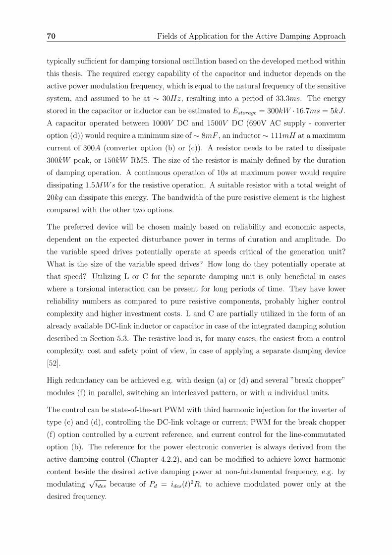
70 Fields of Application for the Active Damping Approach
typically sufficient for damping torsional oscillation based on the developed method within
this thesis. The required energy capability of the capacitor and inductor depends on the
active power modulation frequency, which is equal to the natural frequency of the sensitive
system, and assumed to be at ∼ 30Hz, resulting into a period of 33.3ms. The energy
stored in the capacitor or inductor can be estimated to Estorage = 300kW · 16.7ms = 5kJ .
A capacitor operated between 1000V DC and 1500V DC (690V AC supply - converter
option (d)) would require a minimum size of ∼ 8mF , an inductor ∼ 111mH at a maximum
current of 300A (converter option (b) or (c)). A resistor needs to be rated to dissipate
300kW peak, or 150kW RMS. The size of the resistor is mainly defined by the duration
of damping operation. A continuous operation of 10s at maximum power would require
dissipating 1.5MWs for the resistive operation. A suitable resistor with a total weight of
20kg can dissipate this energy. The bandwidth of the pure resistive element is the highest
compared with the other two options.
The preferred device will be chosen mainly based on reliability and economic aspects,
dependent on the expected disturbance power in terms of duration and amplitude. Do
the variable speed drives potentially operate at speeds critical of the generation unit?
What is the size of the variable speed drives? How long do they potentially operate at
that speed? Utilizing L or C for the separate damping unit is only beneficial in cases
where a torsional interaction can be present for long periods of time. They have lower
reliability numbers as compared to pure resistive components, probably higher control
complexity and higher investment costs. L and C are partially utilized in the form of an
already available DC-link inductor or capacitor in case of the integrated damping solution
described in Section 5.3. The resistive load is, for many cases, the easiest from a control
complexity, cost and safety point of view, in case of applying a separate damping device
[52].
High redundancy can be achieved e.g. with design (a) or (d) and several ”break chopper”
modules (f) in parallel, switching an interleaved pattern, or with n individual units.
The control can be state-of-the-art PWM with third harmonic injection for the inverter of
type (c) and (d), controlling the DC-link voltage or current; PWM for the break chopper
(f) option controlled by a current reference, and current control for the line-commutated
option (b). The reference for the power electronic converter is always derived from the
active damping control (Chapter 4.2.2), and can be modified to achieve lower harmonic
content beside the desired active damping power at non-fundamental frequency, e.g. by
modulating√
ides because of Pd = ides(t)2R, to achieve modulated power only at the
desired frequency.
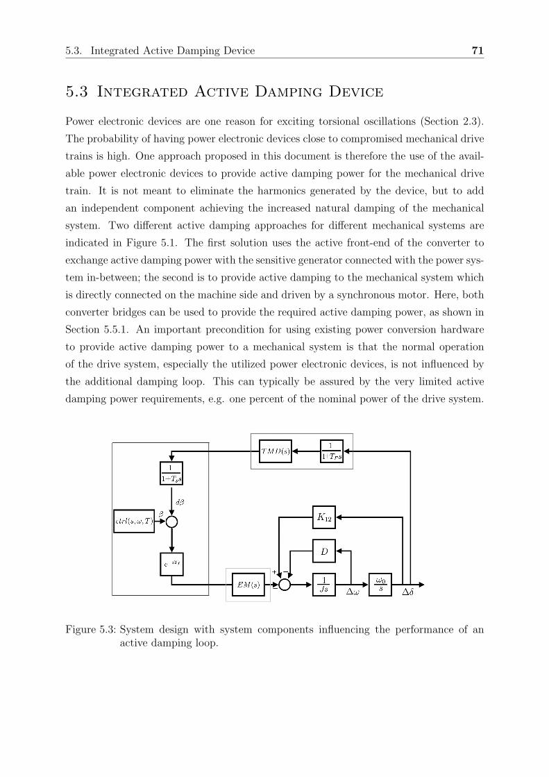
5.3. Integrated Active Damping Device 71
5.3 Integrated Active Damping Device
Power electronic devices are one reason for exciting torsional oscillations (Section 2.3).
The probability of having power electronic devices close to compromised mechanical drive
trains is high. One approach proposed in this document is therefore the use of the avail-
able power electronic devices to provide active damping power for the mechanical drive
train. It is not meant to eliminate the harmonics generated by the device, but to add
an independent component achieving the increased natural damping of the mechanical
system. Two different active damping approaches for different mechanical systems are
indicated in Figure 5.1. The first solution uses the active front-end of the converter to
exchange active damping power with the sensitive generator connected with the power sys-
tem in-between; the second is to provide active damping to the mechanical system which
is directly connected on the machine side and driven by a synchronous motor. Here, both
converter bridges can be used to provide the required active damping power, as shown in
Section 5.5.1. An important precondition for using existing power conversion hardware
to provide active damping power to a mechanical system is that the normal operation
of the drive system, especially the utilized power electronic devices, is not influenced by
the additional damping loop. This can typically be assured by the very limited active
damping power requirements, e.g. one percent of the nominal power of the drive system.
Figure 5.3: System design with system components influencing the performance of anactive damping loop.
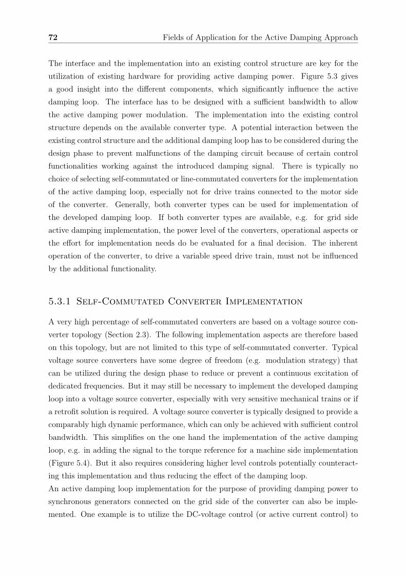
72 Fields of Application for the Active Damping Approach
The interface and the implementation into an existing control structure are key for the
utilization of existing hardware for providing active damping power. Figure 5.3 gives
a good insight into the different components, which significantly influence the active
damping loop. The interface has to be designed with a sufficient bandwidth to allow
the active damping power modulation. The implementation into the existing control
structure depends on the available converter type. A potential interaction between the
existing control structure and the additional damping loop has to be considered during the
design phase to prevent malfunctions of the damping circuit because of certain control
functionalities working against the introduced damping signal. There is typically no
choice of selecting self-commutated or line-commutated converters for the implementation
of the active damping loop, especially not for drive trains connected to the motor side
of the converter. Generally, both converter types can be used for implementation of
the developed damping loop. If both converter types are available, e.g. for grid side
active damping implementation, the power level of the converters, operational aspects or
the effort for implementation needs do be evaluated for a final decision. The inherent
operation of the converter, to drive a variable speed drive train, must not be influenced
by the additional functionality.
5.3.1 Self-Commutated Converter Implementation
A very high percentage of self-commutated converters are based on a voltage source con-
verter topology (Section 2.3). The following implementation aspects are therefore based
on this topology, but are not limited to this type of self-commutated converter. Typical
voltage source converters have some degree of freedom (e.g. modulation strategy) that
can be utilized during the design phase to reduce or prevent a continuous excitation of
dedicated frequencies. But it may still be necessary to implement the developed damping
loop into a voltage source converter, especially with very sensitive mechanical trains or if
a retrofit solution is required. A voltage source converter is typically designed to provide a
comparably high dynamic performance, which can only be achieved with sufficient control
bandwidth. This simplifies on the one hand the implementation of the active damping
loop, e.g. in adding the signal to the torque reference for a machine side implementation
(Figure 5.4). But it also requires considering higher level controls potentially counteract-
ing this implementation and thus reducing the effect of the damping loop.
An active damping loop implementation for the purpose of providing damping power to
synchronous generators connected on the grid side of the converter can also be imple-
mented. One example is to utilize the DC-voltage control (or active current control) to
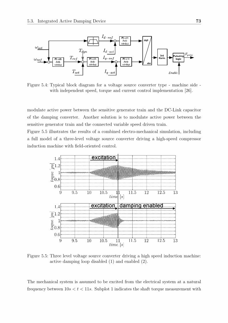
5.3. Integrated Active Damping Device 73
Figure 5.4: Typical block diagram for a voltage source converter type - machine side -with independent speed, torque and current control implementation [26].
modulate active power between the sensitive generator train and the DC-Link capacitor
of the damping converter. Another solution is to modulate active power between the
sensitive generator train and the connected variable speed driven train.
Figure 5.5 illustrates the results of a combined electro-mechanical simulation, including
a full model of a three-level voltage source converter driving a high-speed compressor
induction machine with field-oriented control.
Figure 5.5: Three level voltage source converter driving a high speed induction machine:active damping loop disabled (1) and enabled (2).
The mechanical system is assumed to be excited from the electrical system at a natural
frequency between 10s < t < 11s. Subplot 1 indicates the shaft torque measurement with
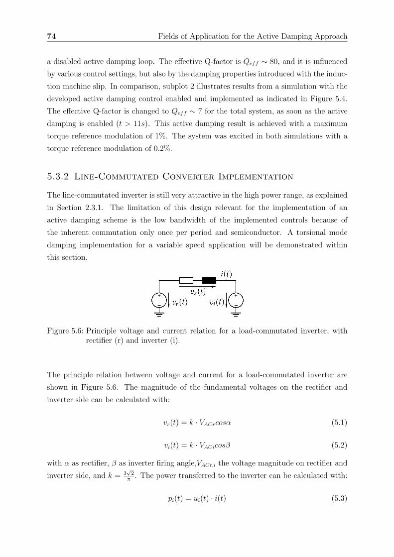
74 Fields of Application for the Active Damping Approach
a disabled active damping loop. The effective Q-factor is Qeff ∼ 80, and it is influenced
by various control settings, but also by the damping properties introduced with the induc-
tion machine slip. In comparison, subplot 2 illustrates results from a simulation with the
developed active damping control enabled and implemented as indicated in Figure 5.4.
The effective Q-factor is changed to Qeff ∼ 7 for the total system, as soon as the active
damping is enabled (t > 11s). This active damping result is achieved with a maximum
torque reference modulation of 1%. The system was excited in both simulations with a
torque reference modulation of 0.2%.
5.3.2 Line-Commutated Converter Implementation
The line-commutated inverter is still very attractive in the high power range, as explained
in Section 2.3.1. The limitation of this design relevant for the implementation of an
active damping scheme is the low bandwidth of the implemented controls because of
the inherent commutation only once per period and semiconductor. A torsional mode
damping implementation for a variable speed application will be demonstrated within
this section.
Figure 5.6: Principle voltage and current relation for a load-commutated inverter, withrectifier (r) and inverter (i).
The principle relation between voltage and current for a load-commutated inverter are
shown in Figure 5.6. The magnitude of the fundamental voltages on the rectifier and
inverter side can be calculated with:
vr(t) = k · VACrcosα (5.1)
vi(t) = k · VACicosβ (5.2)
with α as rectifier, β as inverter firing angle,VACr,i the voltage magnitude on rectifier and
inverter side, and k = 3√
2π
. The power transferred to the inverter can be calculated with:
pi(t) = ui(t) · i(t) (5.3)
5.3. Integrated Active Damping Device 75
Based on Equation 5.3, an active damping power component with natural frequency Ω can
therefore be achieved by modifying the inverter voltage vi(t) or the DC-link current i(t).
The available current control loop would therefore be the preferred point of connection for
the active damping loop, but the control bandwidth of the current control loop typically
only allows effective frequency modulation in the lower frequency range, up to 5..10 Hz,
too low for a general implementation scheme for frequencies in the sub-harmonic range,
but easily applicable and therefore preferred for active damping of natural frequencies
below these limits.
dβ-Modulation
The inverter voltage can be influenced with the firing angle β, which is typically not
derived from a closed loop control, only adapted by looking it up on a table based on the
DC-link current magnitude to achieve power factor values which are as high as possible
(Section 2.3.1). The dynamic required for the equidistant firing angle control is than
realized in hardware. One approach of implementing the active damping loop into a load-
commutated inverter control design therefore modifies the β-angle by exchanging a dβ
signal between damping control loop and load-commutated inverter hardware (see Figure
2.15). The dβ signal is modified based on a signal derived from measurements. The
measurement is filtered to contain just the relevant natural frequency Ω of the connected
mechanical drive train. Equation 5.3 modified by the dβ = β0cos(Ωt) signal can be written
as:
pi(t) = k · VACicos(β + dβ) · i(t) (5.4)
Equation 5.4 is only true with a DC-link current i(t) not influenced by the dβ modulation
for an ideal closed loop current control implementation. A more appropriate implemen-
tation of Equation 5.3 when applying dβ-modulation can therefore be formulated as:
pi(t) = ui(t) · i(t) = (Vdc + vΩcos(Ωt)) · (Idc + iΩcos(Ωt + φ)) (5.5)
uΩ is calculated with:
uΩ = Vdc
∣
∣
∣cos(β + β0) − cos(β − β0)
∣
∣
∣
iΩ is influenced by the size of the smoothing inductor, but also by the current control
performance and can’t be written in simple equations. It will be evaluated for different
control settings in a subsequent section. The current control performance also influences
the source of the modulated power: Two extremes can be derived: (I) ideal current control,
constant DC-link current, no energy at the modulation frequency drawn from the ”energy
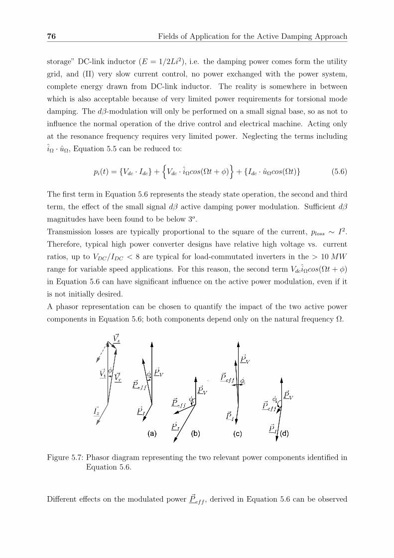
76 Fields of Application for the Active Damping Approach
storage” DC-link inductor (E = 1/2Li2), i.e. the damping power comes form the utility
grid, and (II) very slow current control, no power exchanged with the power system,
complete energy drawn from DC-link inductor. The reality is somewhere in between
which is also acceptable because of very limited power requirements for torsional mode
damping. The dβ-modulation will only be performed on a small signal base, so as not to
influence the normal operation of the drive control and electrical machine. Acting only
at the resonance frequency requires very limited power. Neglecting the terms including
iΩ · uΩ, Equation 5.5 can be reduced to:
pi(t) = Vdc · Idc +
Vdc · iΩcos(Ωt + φ)
+ Idc · uΩcos(Ωt) (5.6)
The first term in Equation 5.6 represents the steady state operation, the second and third
term, the effect of the small signal dβ active damping power modulation. Sufficient dβ
magnitudes have been found to be below 3o.
Transmission losses are typically proportional to the square of the current, ploss ∼ I2.
Therefore, typical high power converter designs have relative high voltage vs. current
ratios, up to VDC/IDC < 8 are typical for load-commutated inverters in the > 10 MW
range for variable speed applications. For this reason, the second term VdciΩcos(Ωt + φ)
in Equation 5.6 can have significant influence on the active power modulation, even if it
is not initially desired.
A phasor representation can be chosen to quantify the impact of the two active power
components in Equation 5.6; both components depend only on the natural frequency Ω.
Figure 5.7: Phasor diagram representing the two relevant power components identified inEquation 5.6.
Different effects on the modulated power ~P eff , derived in Equation 5.6 can be observed
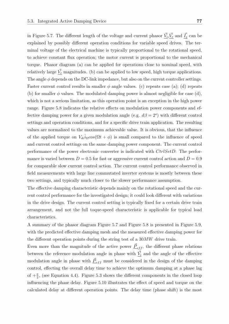
5.3. Integrated Active Damping Device 77
in Figure 5.7. The different length of the voltage and current phasor ~Vi, ~Vr and ~Iz can be
explained by possibly different operation conditions for variable speed drives. The ter-
minal voltage of the electrical machine is typically proportional to the rotational speed,
to achieve constant flux operation; the motor current is proportional to the mechanical
torque. Phasor diagram (a) can be applied for operations close to nominal speed, with
relatively large ~Vr magnitudes. (b) can be applied to low speed, high torque applications.
The angle φ depends on the DC-link impedance, but also on the current controller settings.
Faster current control results in smaller φ angle values. (c) repeats case (a); (d) repeats
(b) for smaller φ values. The modulated damping power is almost negligible for case (d),
which is not a serious limitation, as this operation point is an exception in the high power
range. Figure 5.8 indicates the relative effects on modulation power components and ef-
fective damping power for a given modulation angle (e.g. dβ = 2o) with different control
settings and operation conditions, and for a specific drive train application. The resulting
values are normalized to the maximum achievable value. It is obvious, that the influence
of the applied torque on VdciΩcos(Ωt + φ) is small compared to the influence of speed
and current control settings on the same damping power component. The current control
performance of the power electronic converter is indicated with CtrlSetD: The perfor-
mance is varied between D = 0.5 for fast or aggressive current control action and D = 0.9
for comparable slow current control action. The current control performance observed in
field measurements with large line commutated inverter systems is mostly between these
two settings, and typically much closer to the slower performance assumption.
The effective damping characteristic depends mainly on the rotational speed and the cur-
rent control performance for the investigated design; it could look different with variations
in the drive design. The current control setting is typically fixed for a certain drive train
arrangement, and not the full toque-speed characteristic is applicable for typical load
characteristics.
A summary of the phasor diagram Figure 5.7 and Figure 5.8 is presented in Figure 5.9,
with the predicted effective damping mesh and the measured effective damping power for
the different operation points during the string test of a 30MW drive train.
Even more than the magnitude of the active power ~P eff , the different phase relations
between the reference modulation angle in phase with ~Vi and the angle of the effective
modulation angle in phase with ~P eff must be considered in the design of the damping
control, effecting the overall delay time to achieve the optimum damping at a phase lag
of +π2, (see Equation 4.4). Figure 5.3 shows the different components in the closed loop
influencing the phase delay. Figure 5.10 illustrates the effect of speed and torque on the
calculated delay at different operation points. The delay time (phase shift) is the most
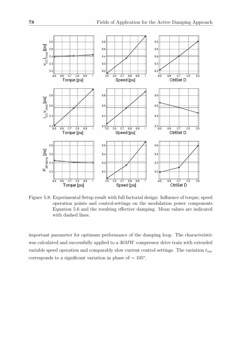
78 Fields of Application for the Active Damping Approach
Figure 5.8: Experimental Setup result with full factorial design: Influence of torque, speedoperation points and control-settings on the modulation power componentsEquation 5.6 and the resulting effective damping. Mean values are indicatedwith dashed lines.
important parameter for optimum performance of the damping loop. The characteristic
was calculated and successfully applied to a 30MW compressor drive train with extended
variable speed operation and comparably slow current control settings. The variation tvar
corresponds to a significant variation in phase of ∼ 105o.
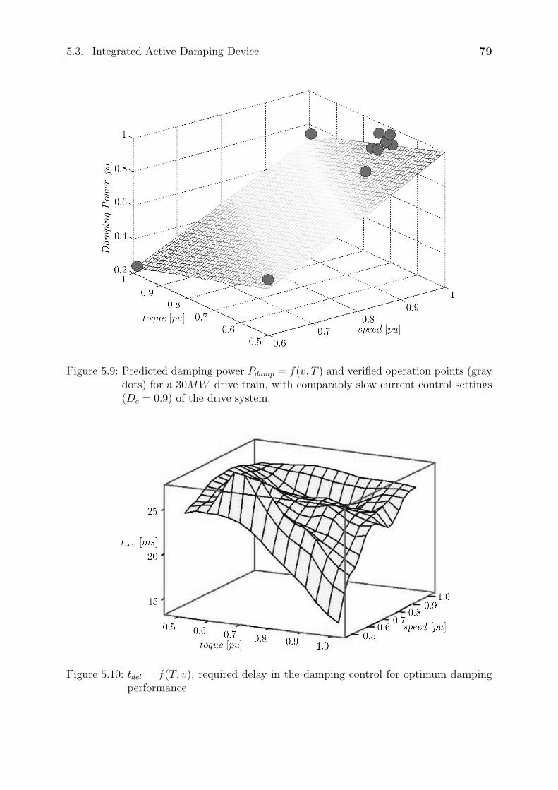
5.3. Integrated Active Damping Device 79
Figure 5.9: Predicted damping power Pdamp = f(v, T ) and verified operation points (graydots) for a 30MW drive train, with comparably slow current control settings(Dc = 0.9) of the drive system.
Figure 5.10: tdel = f(T, v), required delay in the damping control for optimum dampingperformance
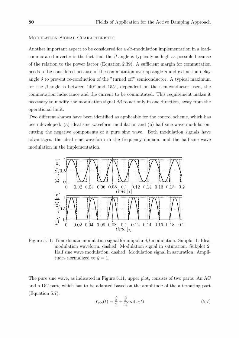
80 Fields of Application for the Active Damping Approach
Modulation Signal Characteristic
Another important aspect to be considered for a dβ-modulation implementation in a load-
commutated inverter is the fact that the β-angle is typically as high as possible because
of the relation to the power factor (Equation 2.39). A sufficient margin for commutation
needs to be considered because of the commutation overlap angle µ and extinction delay
angle δ to prevent re-conduction of the ”turned off” semiconductor. A typical maximum
for the β-angle is between 140o and 155o, dependent on the semiconductor used, the
commutation inductance and the current to be commutated. This requirement makes it
necessary to modify the modulation signal dβ to act only in one direction, away from the
operational limit.
Two different shapes have been identified as applicable for the control scheme, which has
been developed: (a) ideal sine waveform modulation and (b) half sine wave modulation,
cutting the negative components of a pure sine wave. Both modulation signals have
advantages, the ideal sine waveform in the frequency domain, and the half-sine wave
modulation in the implementation.
Figure 5.11: Time domain modulation signal for unipolar dβ-modulation. Subplot 1: Idealmodulation waveform, dashed: Modulation signal in saturation. Subplot 2:Half sine wave modulation, dashed: Modulation signal in saturation. Ampli-tudes normalized to y = 1.
The pure sine wave, as indicated in Figure 5.11, upper plot, consists of two parts: An AC
and a DC-part, which has to be adapted based on the amplitude of the alternating part
(Equation 5.7).
Ysin(t) =y
2+
y
2sin(ω0t) (5.7)

5.3. Integrated Active Damping Device 81
The frequency domain for this plot can be identified in Figure 5.13, upper left plot. The
DC-offset is responsible for a very limited modification of the power angle, dependent on
the required damping power Figure 5.12.
Figure 5.12: Influence of DC-offset on effective power factor, maximum damping powerwith an allowed modulation angle of 2o assumed.
The second, easier to implement, alternative can be seen in Figure 5.11, lower plot, which
can be analyzed by calculating the Fourier series, resulting in:
Yhalf−sin(t) =y
π+
y
2sin(ω0t) −
2y
π
∞∑
k=1
cos(2kω0t)
(2k − 1)(2k + 1)(5.8)
The DC-component in the modulation signal is reduced, but there are additional, even
harmonics produced, e.g. the 2nd, 4th..., see also Figure 5.13, lower left characteristic.
This can be a clear disadvantage, e.g. in case that the second natural frequency is ex-
actly two times the first natural frequency. The signals shown in Figure 5.11 demonstrate
only a snapshot of the modulation signal. The real modulation signal changes the mag-
nitude dynamically, dependent on the alternating torque magnitude in the mechanical
shaft. They can reach lower, but also higher magnitudes, which then result in a saturated
signal waveform unless an anti-windup is implemented. Figure 5.11 gives an idea of satu-
rated signal waveforms (dashed lines). The saturated waveform results for both proposed
shapes, in case of an infinitely high gain, into a pure rectangular shape with its Fourier
series:
Ysat(t) =y
π+
2y
π
∞∑
k=1
sin((2k − 1)ω0t)
2k − 1(5.9)
This waveform includes only odd harmonics, e.g. 3rd, 5th.... Figure 5.13, upper and lower
right, shows the resulting harmonics for the two proposed waveforms in saturation.
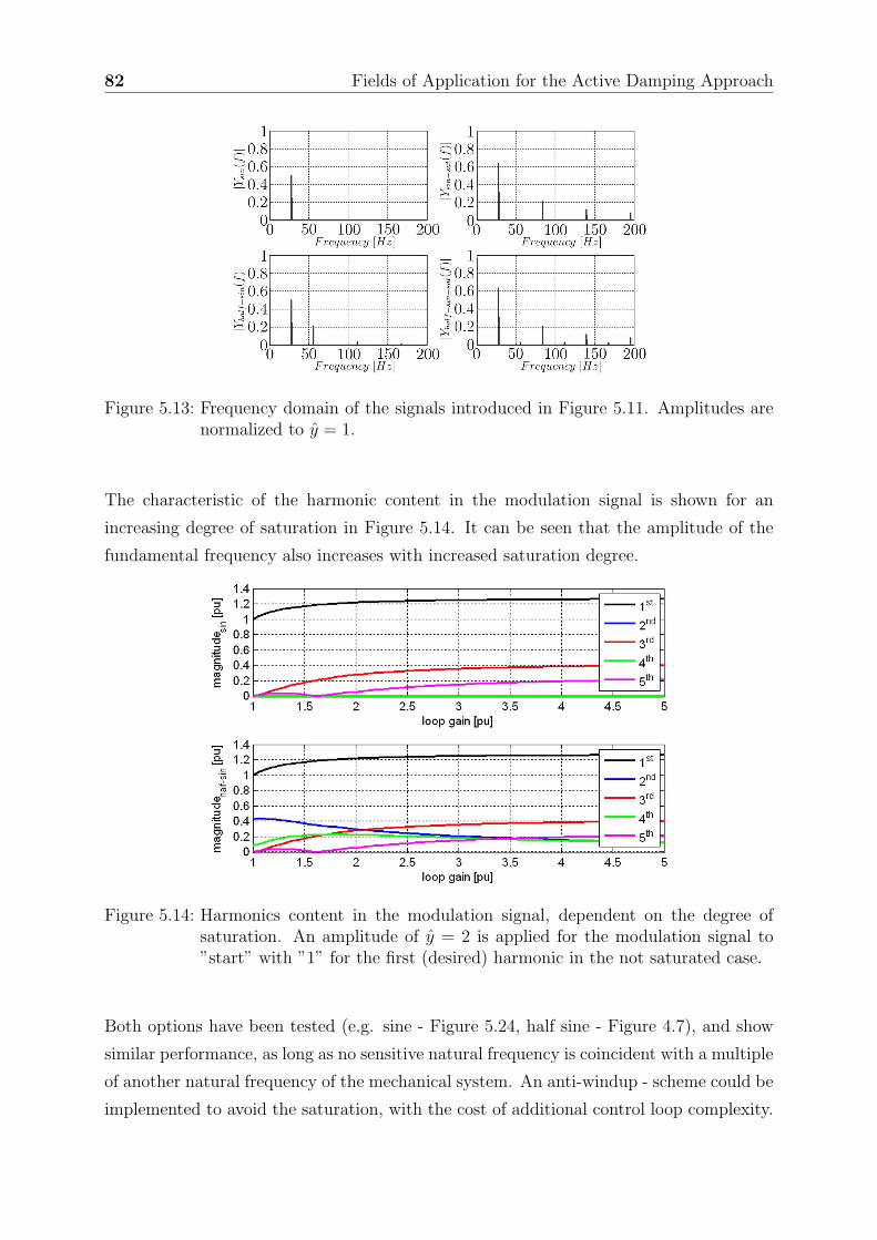
82 Fields of Application for the Active Damping Approach
Figure 5.13: Frequency domain of the signals introduced in Figure 5.11. Amplitudes arenormalized to y = 1.
The characteristic of the harmonic content in the modulation signal is shown for an
increasing degree of saturation in Figure 5.14. It can be seen that the amplitude of the
fundamental frequency also increases with increased saturation degree.
Figure 5.14: Harmonics content in the modulation signal, dependent on the degree ofsaturation. An amplitude of y = 2 is applied for the modulation signal to”start” with ”1” for the first (desired) harmonic in the not saturated case.
Both options have been tested (e.g. sine - Figure 5.24, half sine - Figure 4.7), and show
similar performance, as long as no sensitive natural frequency is coincident with a multiple
of another natural frequency of the mechanical system. An anti-windup - scheme could be
implemented to avoid the saturation, with the cost of additional control loop complexity.
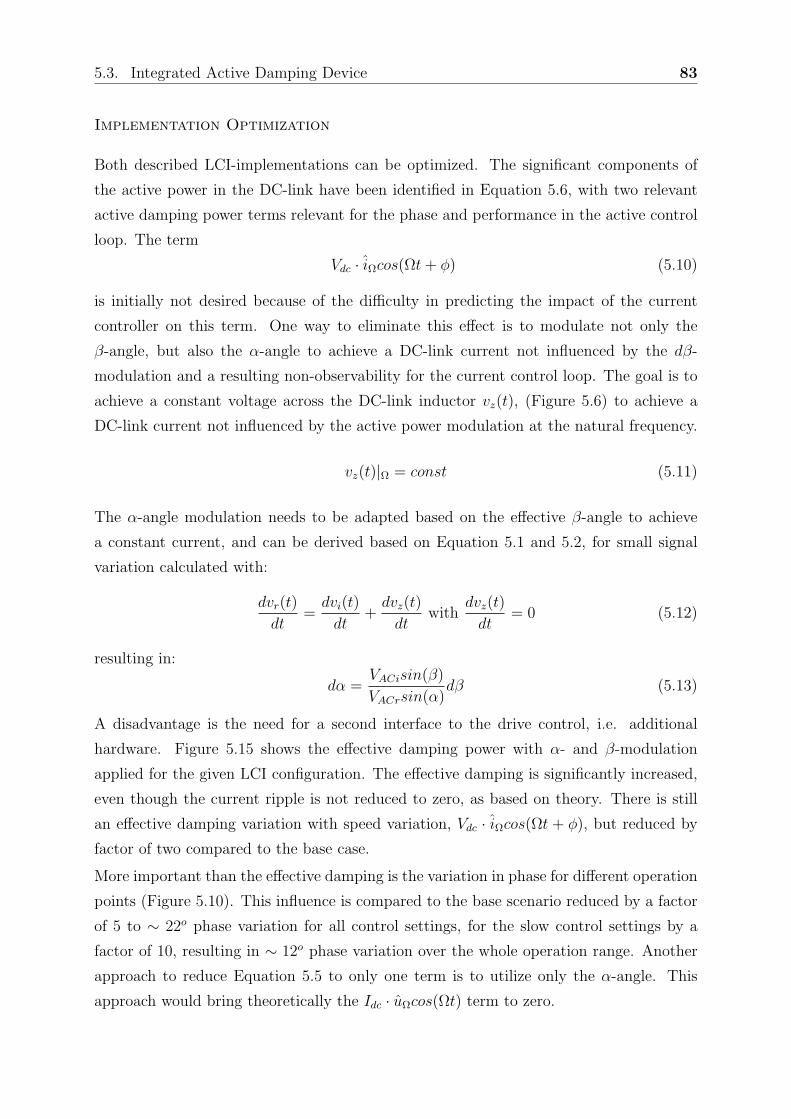
5.3. Integrated Active Damping Device 83
Implementation Optimization
Both described LCI-implementations can be optimized. The significant components of
the active power in the DC-link have been identified in Equation 5.6, with two relevant
active damping power terms relevant for the phase and performance in the active control
loop. The term
Vdc · iΩcos(Ωt + φ) (5.10)
is initially not desired because of the difficulty in predicting the impact of the current
controller on this term. One way to eliminate this effect is to modulate not only the
β-angle, but also the α-angle to achieve a DC-link current not influenced by the dβ-
modulation and a resulting non-observability for the current control loop. The goal is to
achieve a constant voltage across the DC-link inductor vz(t), (Figure 5.6) to achieve a
DC-link current not influenced by the active power modulation at the natural frequency.
vz(t)|Ω = const (5.11)
The α-angle modulation needs to be adapted based on the effective β-angle to achieve
a constant current, and can be derived based on Equation 5.1 and 5.2, for small signal
variation calculated with:
dvr(t)
dt=
dvi(t)
dt+
dvz(t)
dtwith
dvz(t)
dt= 0 (5.12)
resulting in:
dα =VACisin(β)
VACrsin(α)dβ (5.13)
A disadvantage is the need for a second interface to the drive control, i.e. additional
hardware. Figure 5.15 shows the effective damping power with α- and β-modulation
applied for the given LCI configuration. The effective damping is significantly increased,
even though the current ripple is not reduced to zero, as based on theory. There is still
an effective damping variation with speed variation, Vdc · iΩcos(Ωt + φ), but reduced by
factor of two compared to the base case.
More important than the effective damping is the variation in phase for different operation
points (Figure 5.10). This influence is compared to the base scenario reduced by a factor
of 5 to ∼ 22o phase variation for all control settings, for the slow control settings by a
factor of 10, resulting in ∼ 12o phase variation over the whole operation range. Another
approach to reduce Equation 5.5 to only one term is to utilize only the α-angle. This
approach would bring theoretically the Idc · uΩcos(Ωt) term to zero.
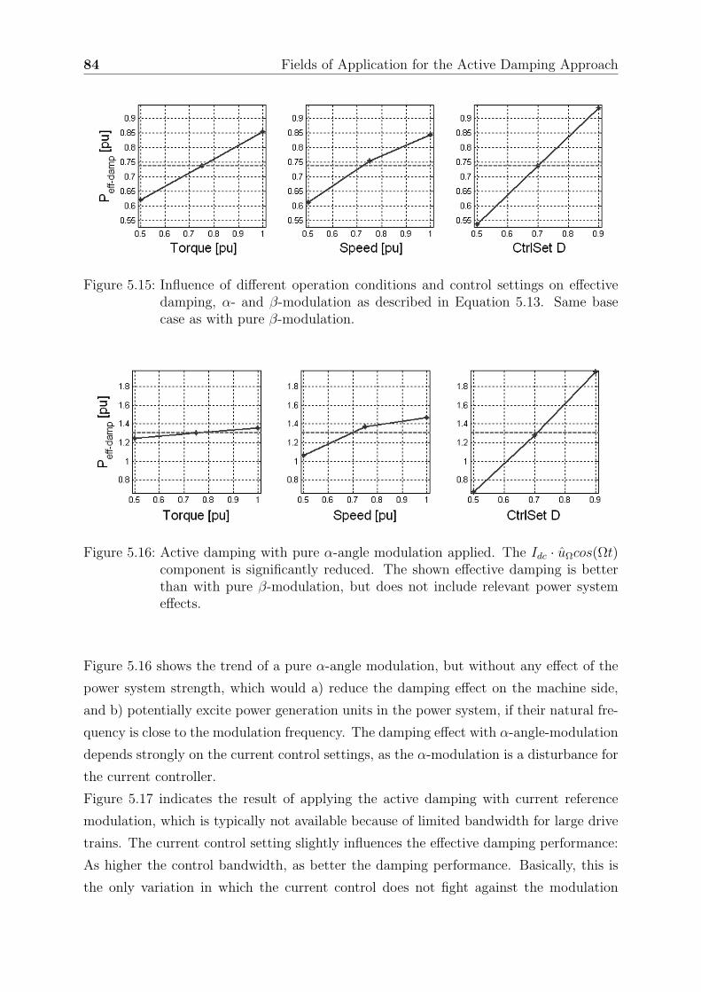
84 Fields of Application for the Active Damping Approach
Figure 5.15: Influence of different operation conditions and control settings on effectivedamping, α- and β-modulation as described in Equation 5.13. Same basecase as with pure β-modulation.
Figure 5.16: Active damping with pure α-angle modulation applied. The Idc · uΩcos(Ωt)component is significantly reduced. The shown effective damping is betterthan with pure β-modulation, but does not include relevant power systemeffects.
Figure 5.16 shows the trend of a pure α-angle modulation, but without any effect of the
power system strength, which would a) reduce the damping effect on the machine side,
and b) potentially excite power generation units in the power system, if their natural fre-
quency is close to the modulation frequency. The damping effect with α-angle-modulation
depends strongly on the current control settings, as the α-modulation is a disturbance for
the current controller.
Figure 5.17 indicates the result of applying the active damping with current reference
modulation, which is typically not available because of limited bandwidth for large drive
trains. The current control setting slightly influences the effective damping performance:
As higher the control bandwidth, as better the damping performance. Basically, this is
the only variation in which the current control does not fight against the modulation
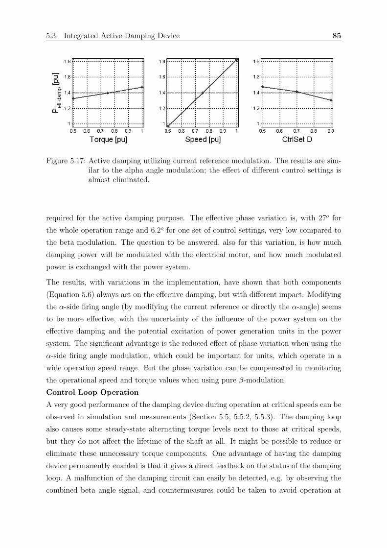
5.3. Integrated Active Damping Device 85
Figure 5.17: Active damping utilizing current reference modulation. The results are sim-ilar to the alpha angle modulation; the effect of different control settings isalmost eliminated.
required for the active damping purpose. The effective phase variation is, with 27o for
the whole operation range and 6.2o for one set of control settings, very low compared to
the beta modulation. The question to be answered, also for this variation, is how much
damping power will be modulated with the electrical motor, and how much modulated
power is exchanged with the power system.
The results, with variations in the implementation, have shown that both components
(Equation 5.6) always act on the effective damping, but with different impact. Modifying
the α-side firing angle (by modifying the current reference or directly the α-angle) seems
to be more effective, with the uncertainty of the influence of the power system on the
effective damping and the potential excitation of power generation units in the power
system. The significant advantage is the reduced effect of phase variation when using the
α-side firing angle modulation, which could be important for units, which operate in a
wide operation speed range. But the phase variation can be compensated in monitoring
the operational speed and torque values when using pure β-modulation.
Control Loop Operation
A very good performance of the damping device during operation at critical speeds can be
observed in simulation and measurements (Section 5.5, 5.5.2, 5.5.3). The damping loop
also causes some steady-state alternating torque levels next to those at critical speeds,
but they do not affect the lifetime of the shaft at all. It might be possible to reduce or
eliminate these unnecessary torque components. One advantage of having the damping
device permanently enabled is that it gives a direct feedback on the status of the damping
loop. A malfunction of the damping circuit can easily be detected, e.g. by observing the
combined beta angle signal, and countermeasures could be taken to avoid operation at
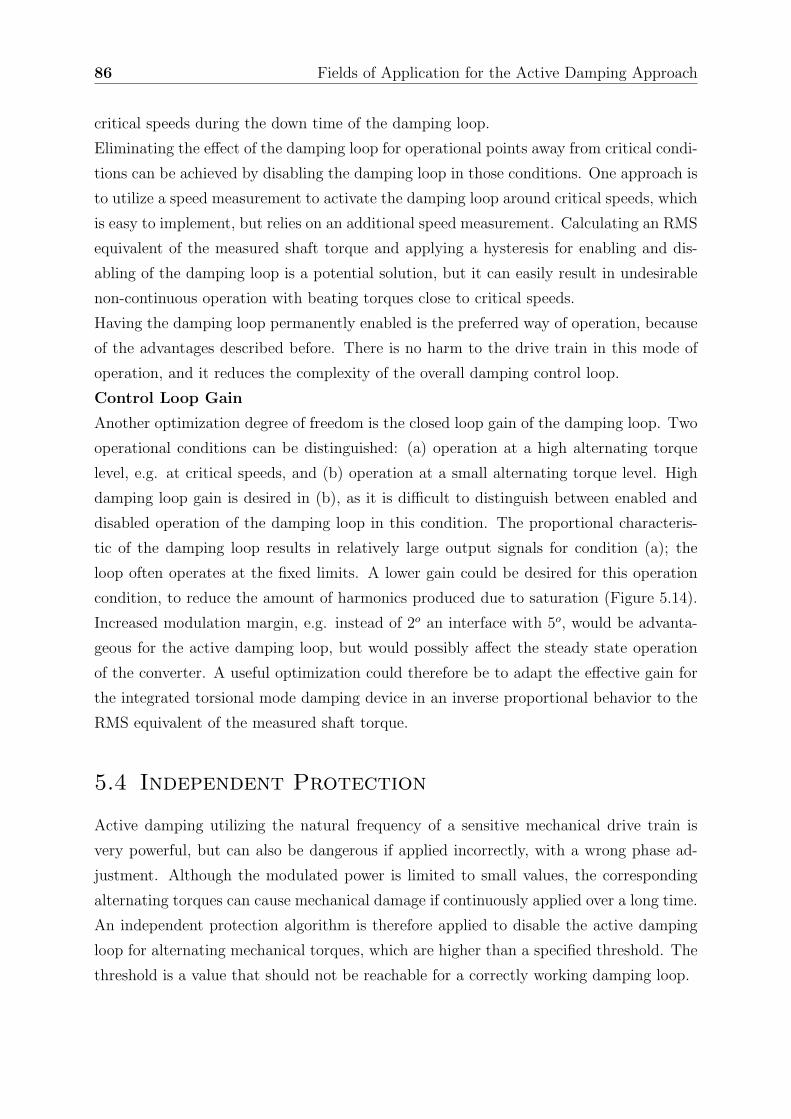
86 Fields of Application for the Active Damping Approach
critical speeds during the down time of the damping loop.
Eliminating the effect of the damping loop for operational points away from critical condi-
tions can be achieved by disabling the damping loop in those conditions. One approach is
to utilize a speed measurement to activate the damping loop around critical speeds, which
is easy to implement, but relies on an additional speed measurement. Calculating an RMS
equivalent of the measured shaft torque and applying a hysteresis for enabling and dis-
abling of the damping loop is a potential solution, but it can easily result in undesirable
non-continuous operation with beating torques close to critical speeds.
Having the damping loop permanently enabled is the preferred way of operation, because
of the advantages described before. There is no harm to the drive train in this mode of
operation, and it reduces the complexity of the overall damping control loop.
Control Loop Gain
Another optimization degree of freedom is the closed loop gain of the damping loop. Two
operational conditions can be distinguished: (a) operation at a high alternating torque
level, e.g. at critical speeds, and (b) operation at a small alternating torque level. High
damping loop gain is desired in (b), as it is difficult to distinguish between enabled and
disabled operation of the damping loop in this condition. The proportional characteris-
tic of the damping loop results in relatively large output signals for condition (a); the
loop often operates at the fixed limits. A lower gain could be desired for this operation
condition, to reduce the amount of harmonics produced due to saturation (Figure 5.14).
Increased modulation margin, e.g. instead of 2o an interface with 5o, would be advanta-
geous for the active damping loop, but would possibly affect the steady state operation
of the converter. A useful optimization could therefore be to adapt the effective gain for
the integrated torsional mode damping device in an inverse proportional behavior to the
RMS equivalent of the measured shaft torque.
5.4 Independent Protection
Active damping utilizing the natural frequency of a sensitive mechanical drive train is
very powerful, but can also be dangerous if applied incorrectly, with a wrong phase ad-
justment. Although the modulated power is limited to small values, the corresponding
alternating torques can cause mechanical damage if continuously applied over a long time.
An independent protection algorithm is therefore applied to disable the active damping
loop for alternating mechanical torques, which are higher than a specified threshold. The
threshold is a value that should not be reachable for a correctly working damping loop.
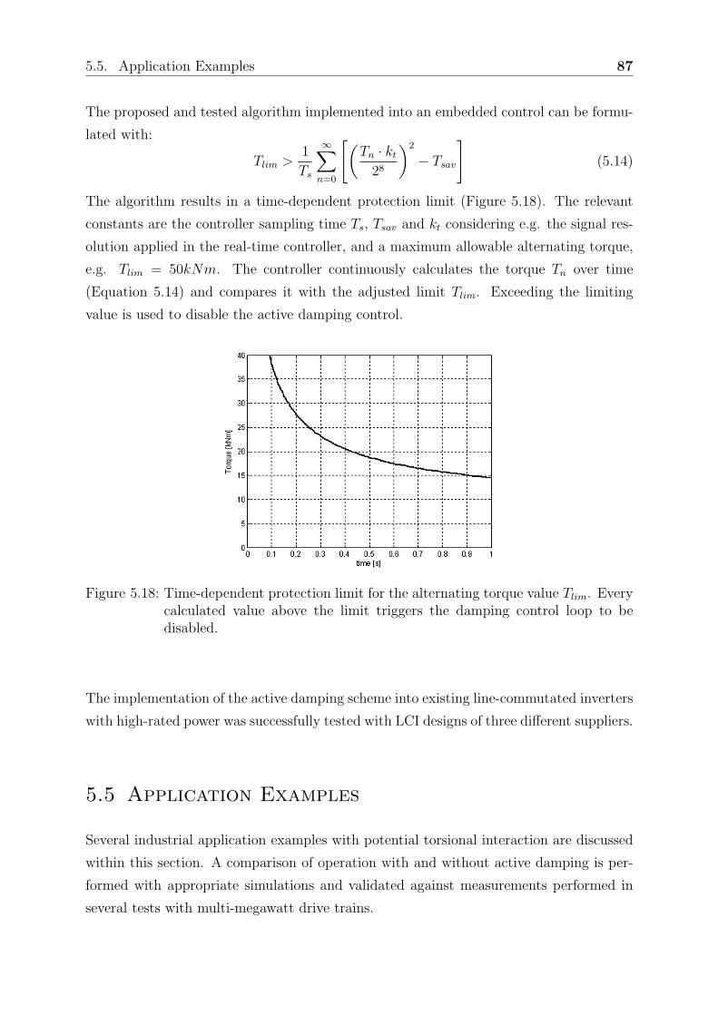
5.5. Application Examples 87
The proposed and tested algorithm implemented into an embedded control can be formu-
lated with:
Tlim >1
Ts
∞∑
n=0
[
(
Tn · kt
28
)2
− Tsav
]
(5.14)
The algorithm results in a time-dependent protection limit (Figure 5.18). The relevant
constants are the controller sampling time Ts, Tsav and kt considering e.g. the signal res-
olution applied in the real-time controller, and a maximum allowable alternating torque,
e.g. Tlim = 50kNm. The controller continuously calculates the torque Tn over time
(Equation 5.14) and compares it with the adjusted limit Tlim. Exceeding the limiting
value is used to disable the active damping control.
Figure 5.18: Time-dependent protection limit for the alternating torque value Tlim. Everycalculated value above the limit triggers the damping control loop to bedisabled.
The implementation of the active damping scheme into existing line-commutated inverters
with high-rated power was successfully tested with LCI designs of three different suppliers.
5.5 Application Examples
Several industrial application examples with potential torsional interaction are discussed
within this section. A comparison of operation with and without active damping is per-
formed with appropriate simulations and validated against measurements performed in
several tests with multi-megawatt drive trains.

88 Fields of Application for the Active Damping Approach
5.5.1 Damping Results for Variable Speed Drives
The successful application of the developed damping method for large industrial drive
trains is an important achievement within the thesis. The various implementation steps
have been discussed in previous sections. Simulation results for a 30MW drive train will
now be discussed and compared to measurements. An LCI produces variable pulsating
torque components in variable speed operation, based on Figure 2.19. The effect on the
mechanical drive train will be shown in the following simulation and measurement results.
Figure 5.19: 12/12-Pulse LCI design feeding a 6-phase synchronous motor
A single line diagram of the electrical system investigated within this subsection is given
in Figure 5.19. A 12-pulse LCI is utilized to allow operation in a wide speed range of
50% to 105% of nominal speed at nominal torque. Several critical speeds are within this
operation range.
Figure 5.20 illustrates the reaction of the mechanical system to a constant speed ramp with
2.5 rpm/s when running through a critical speed (speed = 0.952p.u.). The alternating
torque amplitude increases before and after the resonance point, as the quality of the
resonance is not infinite. The magnitude of the alternating torque and therefore the
stress level depends on the speed ramp applied. A lower speed ramp results in more
periods of excitation at the natural frequency; higher magnitudes can be observed. In
the given arrangement, the magnitude already exceeds the allowed continuous alternating
torque level of the coupling. The speed reference is usually set by the process, e.g. by
the required operational temperature and pressure of a Liquid Natural Gas compression
train. Running through critical speeds or even operation at critical speed can therefore
not always be prevented for variable speed operation (Campbell Diagram - Figure 3.1),
with potential negative effects for the mechanical drive train. The alternating torque

5.5. Application Examples 89
does not continuously decrease after passing the natural frequency, which is caused by
the interharmonic content with increasing frequency: A beating effect excites and damps
the torsional oscillation depending on the phase relation between the harmonic, which
increases in frequency, and the present torsional oscillation at the mechanical natural
frequency. The effective alternating torque decreases with increasing distance between
the interharmonic frequency and the natural frequency of the mechanical system.
Figure 5.20: Simulation result: Variable speed operation of an electrically driven drivetrain. An increased level of dynamic torques can be detected while passinga critical speed.
A waterfall calculation applied to the mechanical torque enables the identification of the
interharmonics responsible for the torsional interaction - Figure 5.21. The abscissa axis
represents the time measured in seconds, the ordinate axis the frequency content and the
color in the diagram represents the amplitude of the frequency components, with larger
amplitude for colors with larger wavelength. It can clearly be seen, that the electrical
frequency component with |12fg − 12fm| crosses the natural frequency at 29Hz, resulting
in high alternating torque components at that frequency around t = 12s. Running through
a critical speed with the same ramp as before, but with torsional damping device enabled
after t = 12.5s, is investigated in Figure 5.22 and Figure 5.23. The damping device would
typically always be enabled during operation; this run is only for demonstration of the
damping performance. The alternating torque at natural frequency is almost gone after
activation of the damping device. A kind of ”white noise” around the critical speed can
be identified in the frequency plot.
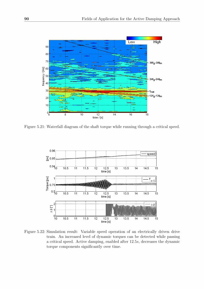
90 Fields of Application for the Active Damping Approach
Figure 5.21: Waterfall diagram of the shaft torque while running through a critical speed.
Figure 5.22: Simulation result: Variable speed operation of an electrically driven drivetrain. An increased level of dynamic torques can be detected while passinga critical speed. Active damping, enabled after 12.5s, decreases the dynamictorque components significantly over time.
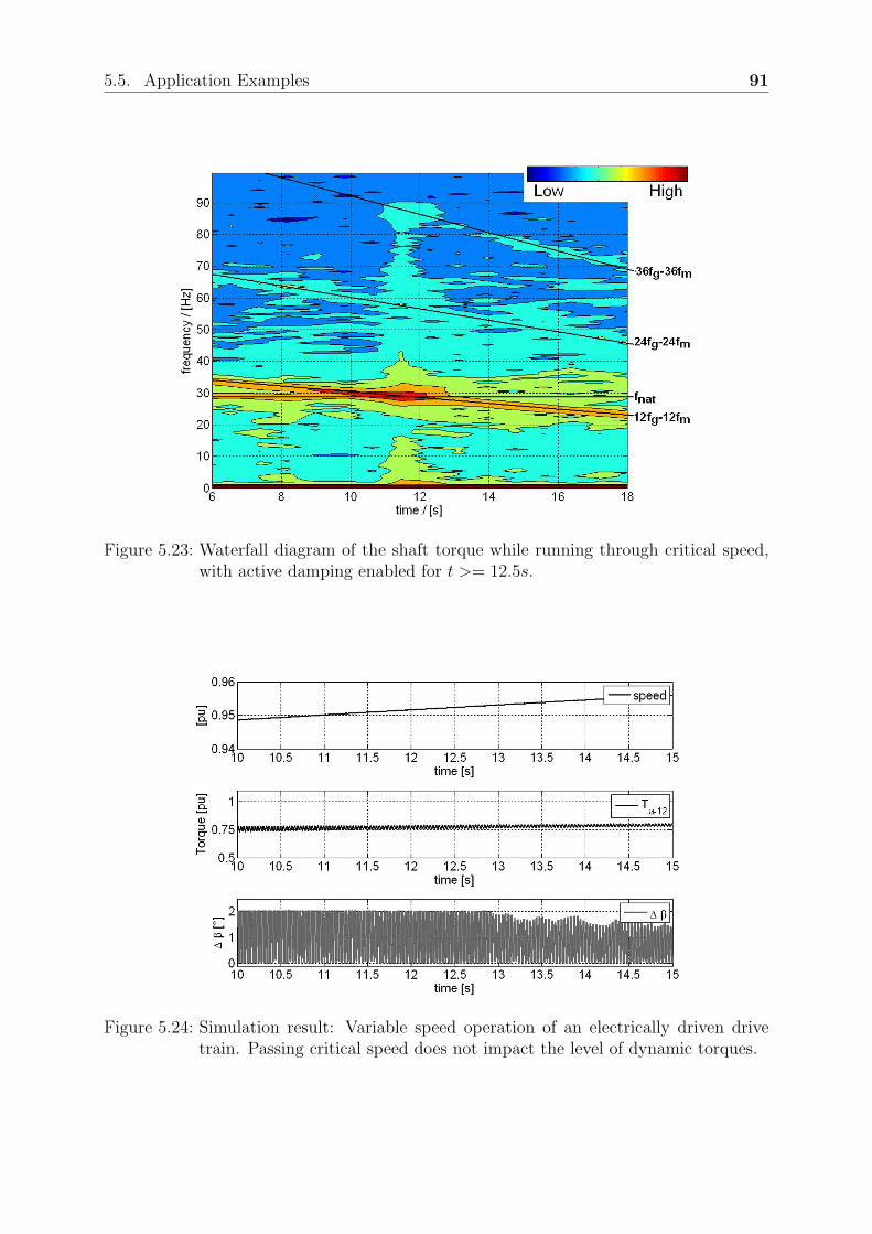
5.5. Application Examples 91
Figure 5.23: Waterfall diagram of the shaft torque while running through critical speed,with active damping enabled for t >= 12.5s.
Figure 5.24: Simulation result: Variable speed operation of an electrically driven drivetrain. Passing critical speed does not impact the level of dynamic torques.

92 Fields of Application for the Active Damping Approach
The run through critical speed with damping fully enabled is shown in Figure 5.24. The
alternating torque is limited to a value well within the limits set for permanent operation.
The same series of runs has been performed with a real 30MW synchronous motor driven
compressor train during a string test. The effective alternating torque corresponds well
to the simulated result shown in Figure 5.20.
Figure 5.25: Measurement result: Variable speed operation through critical speed (be-low nominal speed): The dynamic torque level is increasing to unacceptablevalues.
Figure 5.25 illustrates the run through a critical speed with the damping device disabled.
The alternating torque is increasing to unacceptable values within a second. The same
run performed with active damping enabled is shown in Figure 5.26. The alternating
torque is significantly reduced. The reduction is lower than in the simulation because a
lower gain has been applied in the tests. Such strong damping effects are not required
in real systems. The damping device is meant to provide additional damping at critical
speeds to be able to run through, or even at critical speed while staying well below the
alternating torque limit of the drive train, and not reducing the alternating torque to
zero. The difference between simulation and reality can be found with different gains in
the damping control loop, but is also due to the existence of additional ”converter torque
noise” in the real system, e.g. due to switching effects, which have been measured in all
operation conditions. Lower alternating torque could be achieved with higher damping
power and higher gain in the damping loop. The string tests performed with a 30MW
compression train with ITMD control also included fault analyses for the damping control.
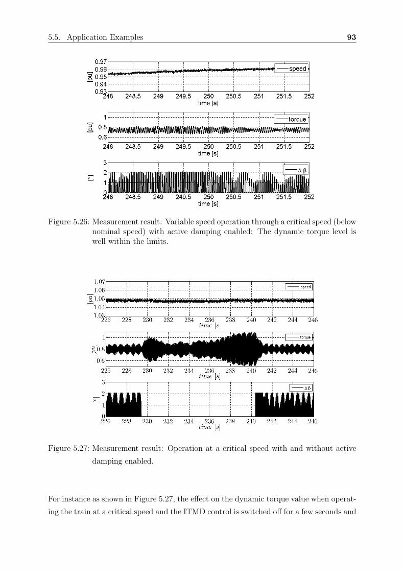
5.5. Application Examples 93
Figure 5.26: Measurement result: Variable speed operation through a critical speed (belownominal speed) with active damping enabled: The dynamic torque level iswell within the limits.
Figure 5.27: Measurement result: Operation at a critical speed with and without active
damping enabled.
For instance as shown in Figure 5.27, the effect on the dynamic torque value when operat-
ing the train at a critical speed and the ITMD control is switched off for a few seconds and
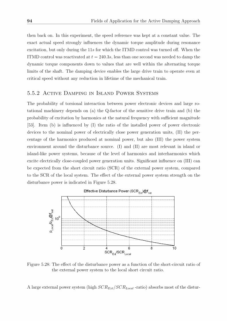
94 Fields of Application for the Active Damping Approach
then back on. In this experiment, the speed reference was kept at a constant value. The
exact actual speed strongly influences the dynamic torque amplitude during resonance
excitation, but only during the 11s for which the ITMD control was turned off. When the
ITMD control was reactivated at t = 240.3s, less than one second was needed to damp the
dynamic torque components down to values that are well within the alternating torque
limits of the shaft. The damping device enables the large drive train to operate even at
critical speed without any reduction in lifetime of the mechanical train.
5.5.2 Active Damping in Island Power Systems
The probability of torsional interaction between power electronic devices and large ro-
tational machinery depends on (a) the Q-factor of the sensitive drive train and (b) the
probability of excitation by harmonics at the natural frequency with sufficient magnitude
[53]. Item (b) is influenced by (I) the ratio of the installed power of power electronic
devices to the nominal power of electrically close power generation units, (II) the per-
centage of the harmonics produced at nominal power, but also (III) the power system
environment around the disturbance source. (I) and (II) are most relevant in island or
island-like power systems, because of the level of harmonics and interharmonics which
excite electrically close-coupled power generation units. Significant influence on (III) can
be expected from the short circuit ratio (SCR) of the external power system, compared
to the SCR of the local system. The effect of the external power system strength on the
disturbance power is indicated in Figure 5.28.
Figure 5.28: The effect of the disturbance power as a function of the short-circuit ratio ofthe external power system to the local short circuit ratio.
A large external power system (high SCRExt/SCRLocal -ratio) absorbs most of the distur-
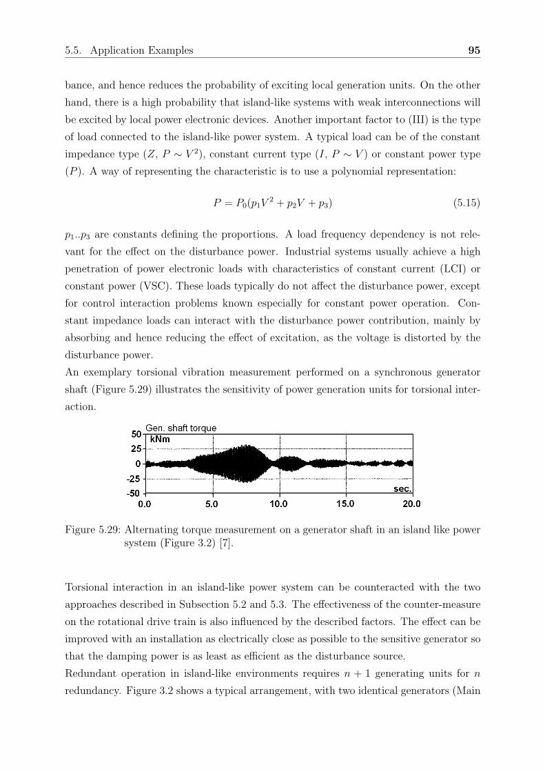
5.5. Application Examples 95
bance, and hence reduces the probability of exciting local generation units. On the other
hand, there is a high probability that island-like systems with weak interconnections will
be excited by local power electronic devices. Another important factor to (III) is the type
of load connected to the island-like power system. A typical load can be of the constant
impedance type (Z, P ∼ V 2), constant current type (I, P ∼ V ) or constant power type
(P ). A way of representing the characteristic is to use a polynomial representation:
P = P0(p1V2 + p2V + p3) (5.15)
p1..p3 are constants defining the proportions. A load frequency dependency is not rele-
vant for the effect on the disturbance power. Industrial systems usually achieve a high
penetration of power electronic loads with characteristics of constant current (LCI) or
constant power (VSC). These loads typically do not affect the disturbance power, except
for control interaction problems known especially for constant power operation. Con-
stant impedance loads can interact with the disturbance power contribution, mainly by
absorbing and hence reducing the effect of excitation, as the voltage is distorted by the
disturbance power.
An exemplary torsional vibration measurement performed on a synchronous generator
shaft (Figure 5.29) illustrates the sensitivity of power generation units for torsional inter-
action.
Figure 5.29: Alternating torque measurement on a generator shaft in an island like powersystem (Figure 3.2) [7].
Torsional interaction in an island-like power system can be counteracted with the two
approaches described in Subsection 5.2 and 5.3. The effectiveness of the counter-measure
on the rotational drive train is also influenced by the described factors. The effect can be
improved with an installation as electrically close as possible to the sensitive generator so
that the damping power is as least as efficient as the disturbance source.
Redundant operation in island-like environments requires n + 1 generating units for n
redundancy. Figure 3.2 shows a typical arrangement, with two identical generators (Main
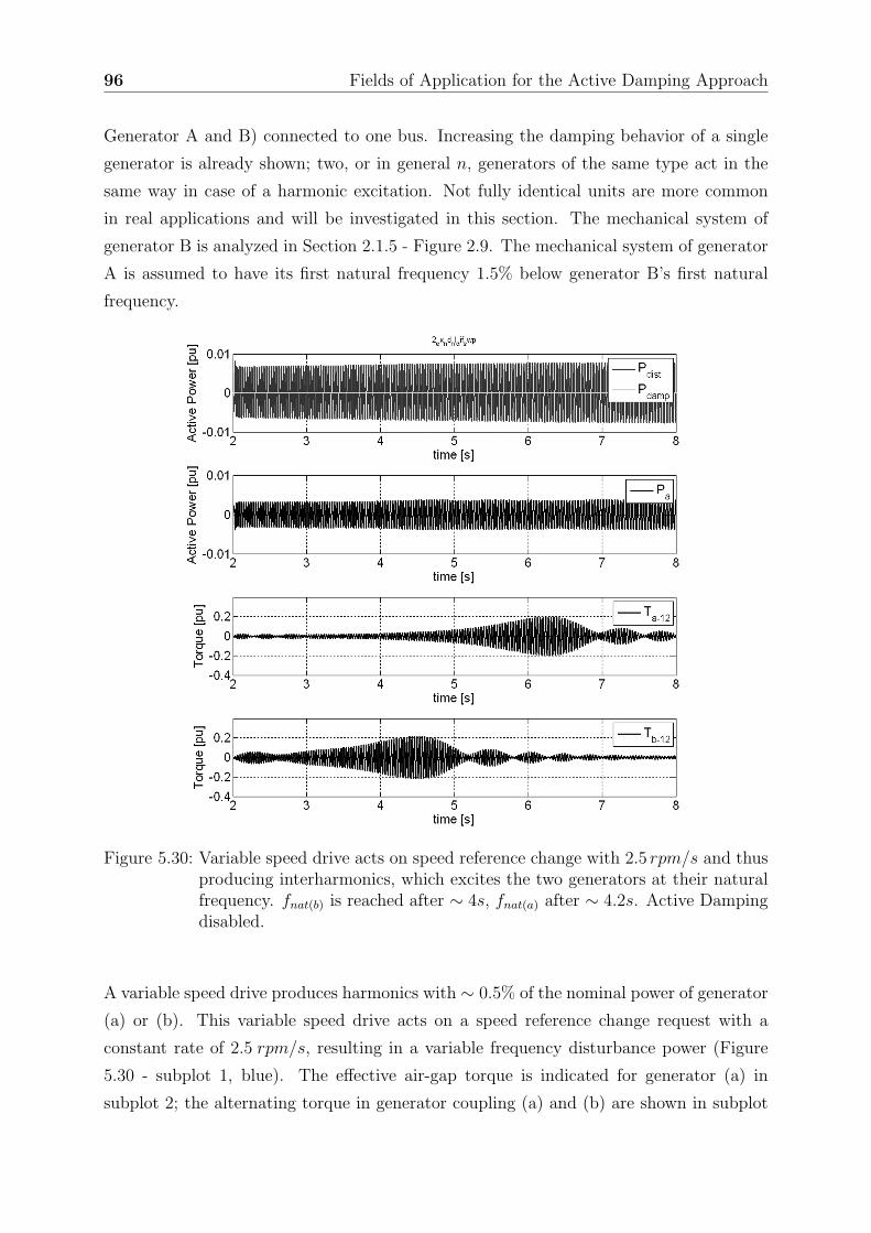
96 Fields of Application for the Active Damping Approach
Generator A and B) connected to one bus. Increasing the damping behavior of a single
generator is already shown; two, or in general n, generators of the same type act in the
same way in case of a harmonic excitation. Not fully identical units are more common
in real applications and will be investigated in this section. The mechanical system of
generator B is analyzed in Section 2.1.5 - Figure 2.9. The mechanical system of generator
A is assumed to have its first natural frequency 1.5% below generator B’s first natural
frequency.
Figure 5.30: Variable speed drive acts on speed reference change with 2.5 rpm/s and thusproducing interharmonics, which excites the two generators at their naturalfrequency. fnat(b) is reached after ∼ 4s, fnat(a) after ∼ 4.2s. Active Dampingdisabled.
A variable speed drive produces harmonics with ∼ 0.5% of the nominal power of generator
(a) or (b). This variable speed drive acts on a speed reference change request with a
constant rate of 2.5 rpm/s, resulting in a variable frequency disturbance power (Figure
5.30 - subplot 1, blue). The effective air-gap torque is indicated for generator (a) in
subplot 2; the alternating torque in generator coupling (a) and (b) are shown in subplot
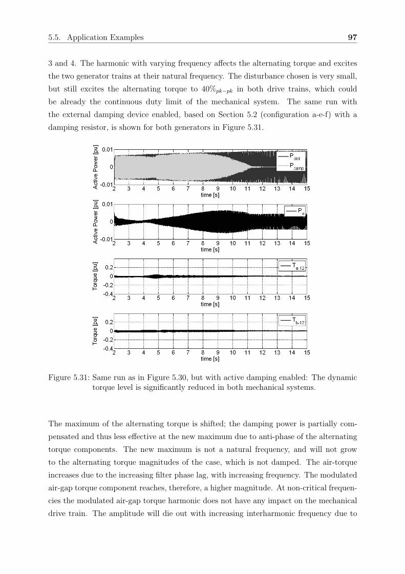
5.5. Application Examples 97
3 and 4. The harmonic with varying frequency affects the alternating torque and excites
the two generator trains at their natural frequency. The disturbance chosen is very small,
but still excites the alternating torque to 40%pk−pk in both drive trains, which could
be already the continuous duty limit of the mechanical system. The same run with
the external damping device enabled, based on Section 5.2 (configuration a-e-f) with a
damping resistor, is shown for both generators in Figure 5.31.
Figure 5.31: Same run as in Figure 5.30, but with active damping enabled: The dynamictorque level is significantly reduced in both mechanical systems.
The maximum of the alternating torque is shifted; the damping power is partially com-
pensated and thus less effective at the new maximum due to anti-phase of the alternating
torque components. The new maximum is not a natural frequency, and will not grow
to the alternating torque magnitudes of the case, which is not damped. The air-torque
increases due to the increasing filter phase lag, with increasing frequency. The modulated
air-gap torque component reaches, therefore, a higher magnitude. At non-critical frequen-
cies the modulated air-gap torque harmonic does not have any impact on the mechanical
drive train. The amplitude will die out with increasing interharmonic frequency due to
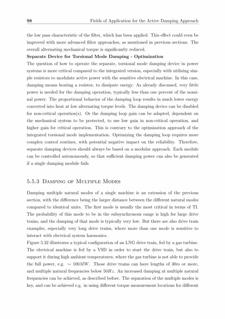
98 Fields of Application for the Active Damping Approach
the low pass characteristic of the filter, which has been applied. This effect could even be
improved with more advanced filter approaches, as mentioned in previous sections. The
overall alternating mechanical torque is significantly reduced.
Separate Device for Torsional Mode Damping - Optimization
The question of how to operate the separate, torsional mode damping device in power
systems is more critical compared to the integrated version, especially with utilizing sim-
ple resistors to modulate active power with the sensitive electrical machine. In this case,
damping means heating a resistor, to dissipate energy. As already discussed, very little
power is needed for the damping operation, typically less than one percent of the nomi-
nal power. The proportional behavior of the damping loop results in much lower energy
converted into heat at low alternating torque levels. The damping device can be disabled
for non-critical operation(s). Or the damping loop gain can be adapted, dependent on
the mechanical system to be protected, to use low gain in non-critical operation, and
higher gain for critical operation. This is contrary to the optimization approach of the
integrated torsional mode implementation. Optimizing the damping loop requires more
complex control routines, with potential negative impact on the reliability. Therefore,
separate damping devices should always be based on a modular approach. Each module
can be controlled autonomously, so that sufficient damping power can also be generated
if a single damping module fails.
5.5.3 Damping of Multiple Modes
Damping multiple natural modes of a single machine is an extension of the previous
section, with the difference being the larger distance between the different natural modes
compared to identical units. The first mode is usually the most critical in terms of TI.
The probability of this mode to be in the subsynchronous range is high for large drive
trains, and the damping of that mode is typically very low. But there are also drive train
examples, especially very long drive trains, where more than one mode is sensitive to
interact with electrical system harmonics.
Figure 5.32 illustrates a typical configuration of an LNG drive train, fed by a gas turbine.
The electrical machine is fed by a VSD in order to start the drive train, but also to
support it during high ambient temperatures, where the gas turbine is not able to provide
the full power, e.g. ∼ 100MW . Those drive trains can have lengths of 30m or more,
and multiple natural frequencies below 50Hz. An increased damping at multiple natural
frequencies can be achieved, as described before. The separation of the multiple modes is
key, and can be achieved e.g. in using different torque measurement locations for different
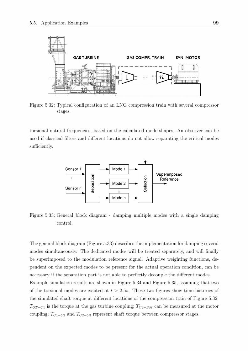
5.5. Application Examples 99
Figure 5.32: Typical configuration of an LNG compression train with several compressorstages.
torsional natural frequencies, based on the calculated mode shapes. An observer can be
used if classical filters and different locations do not allow separating the critical modes
sufficiently.
Figure 5.33: General block diagram - damping multiple modes with a single damping
control.
The general block diagram (Figure 5.33) describes the implementation for damping several
modes simultaneously. The dedicated modes will be treated separately, and will finally
be superimposed to the modulation reference signal. Adaptive weighting functions, de-
pendent on the expected modes to be present for the actual operation condition, can be
necessary if the separation part is not able to perfectly decouple the different modes.
Example simulation results are shown in Figure 5.34 and Figure 5.35, assuming that two
of the torsional modes are excited at t > 2.5s. These two figures show time histories of
the simulated shaft torque at different locations of the compression train of Figure 5.32:
TGT−C1 is the torque at the gas turbine coupling; TC3−EM can be measured at the motor
coupling; TC1−C2 and TC2−C3 represent shaft torque between compressor stages.
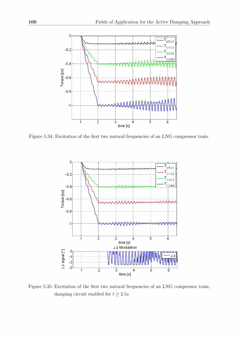
100 Fields of Application for the Active Damping Approach
Figure 5.34: Excitation of the first two natural frequencies of an LNG compressor train.
Figure 5.35: Excitation of the first two natural frequencies of an LNG compressor train,
damping circuit enabled for t ≥ 2.5s.
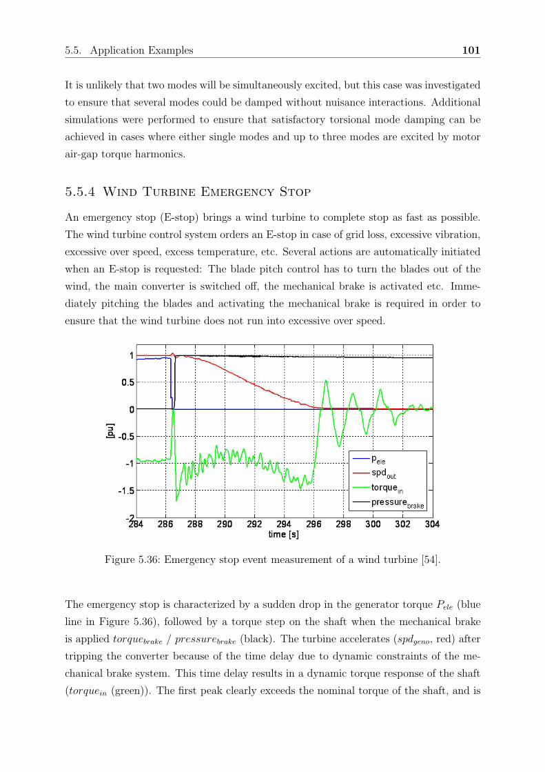
5.5. Application Examples 101
It is unlikely that two modes will be simultaneously excited, but this case was investigated
to ensure that several modes could be damped without nuisance interactions. Additional
simulations were performed to ensure that satisfactory torsional mode damping can be
achieved in cases where either single modes and up to three modes are excited by motor
air-gap torque harmonics.
5.5.4 Wind Turbine Emergency Stop
An emergency stop (E-stop) brings a wind turbine to complete stop as fast as possible.
The wind turbine control system orders an E-stop in case of grid loss, excessive vibration,
excessive over speed, excess temperature, etc. Several actions are automatically initiated
when an E-stop is requested: The blade pitch control has to turn the blades out of the
wind, the main converter is switched off, the mechanical brake is activated etc. Imme-
diately pitching the blades and activating the mechanical brake is required in order to
ensure that the wind turbine does not run into excessive over speed.
Figure 5.36: Emergency stop event measurement of a wind turbine [54].
The emergency stop is characterized by a sudden drop in the generator torque Pele (blue
line in Figure 5.36), followed by a torque step on the shaft when the mechanical brake
is applied torquebrake / pressurebrake (black). The turbine accelerates (spdgeno, red) after
tripping the converter because of the time delay due to dynamic constraints of the me-
chanical brake system. This time delay results in a dynamic torque response of the shaft
(torquein (green)). The first peak clearly exceeds the nominal torque of the shaft, and is
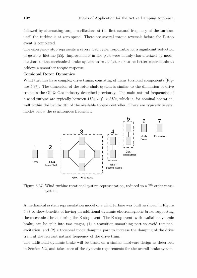
102 Fields of Application for the Active Damping Approach
followed by alternating torque oscillations at the first natural frequency of the turbine,
until the turbine is at zero speed. There are several torque reversals before the E-stop
event is completed.
The emergency stop represents a severe load cycle, responsible for a significant reduction
of gearbox lifetime [55]. Improvements in the past were mainly characterized by modi-
fications to the mechanical brake system to react faster or to be better controllable to
achieve a smoother torque response.
Torsional Rotor Dynamics
Wind turbines have complex drive trains, consisting of many torsional components (Fig-
ure 5.37). The dimension of the rotor shaft system is similar to the dimension of drive
trains in the Oil & Gas industry described previously. The main natural frequencies of
a wind turbine are typically between 1Hz < f1 < 3Hz, which is, for nominal operation,
well within the bandwidth of the available torque controller. There are typically several
modes below the synchronous frequency.
Figure 5.37: Wind turbine rotational system representation, reduced to a 7th order mass-system.
A mechanical system representation model of a wind turbine was built as shown in Figure
5.37 to show benefits of having an additional dynamic electromagnetic brake supporting
the mechanical brake during the E-stop event. The E-stop event, with available dynamic
brake, can be split into two stages, (1) a transition smoothing part to avoid torsional
excitation, and (2) a torsional mode damping part to increase the damping of the drive
train at the relevant natural frequency of the drive train.
The additional dynamic brake will be based on a similar hardware design as described
in Section 5.2, and takes care of the dynamic requirements for the overall brake system.
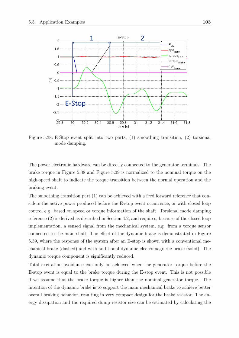
5.5. Application Examples 103
Figure 5.38: E-Stop event split into two parts, (1) smoothing transition, (2) torsionalmode damping.
The power electronic hardware can be directly connected to the generator terminals. The
brake torque in Figure 5.38 and Figure 5.39 is normalized to the nominal torque on the
high-speed shaft to indicate the torque transition between the normal operation and the
braking event.
The smoothing transition part (1) can be achieved with a feed forward reference that con-
siders the active power produced before the E-stop event occurrence, or with closed loop
control e.g. based on speed or torque information of the shaft. Torsional mode damping
reference (2) is derived as described in Section 4.2, and requires, because of the closed loop
implementation, a sensed signal from the mechanical system, e.g. from a torque sensor
connected to the main shaft. The effect of the dynamic brake is demonstrated in Figure
5.39, where the response of the system after an E-stop is shown with a conventional me-
chanical brake (dashed) and with additional dynamic electromagnetic brake (solid). The
dynamic torque component is significantly reduced.
Total excitation avoidance can only be achieved when the generator torque before the
E-stop event is equal to the brake torque during the E-stop event. This is not possible
if we assume that the brake torque is higher than the nominal generator torque. The
intention of the dynamic brake is to support the main mechanical brake to achieve better
overall braking behavior, resulting in very compact design for the brake resistor. The en-
ergy dissipation and the required dump resistor size can be estimated by calculating the

104 Fields of Application for the Active Damping Approach
Figure 5.39: Simulation of the resulting torque during an E-Stop event with and withoutdynamic brake.
surface below the magenta dynamic brake line. The major energy needs to be dissipated
during the initial smoothing transition phase, where the dynamic brake power can reach
the nominal power. The smoothing phase typically lasts less than 500ms. The power
electronic and the dump resistor can be designed with a certain overload capability, to
withstand the peak power without rating it to nominal power. The torsional mode damp-
ing has much lower power requirements, as it operates at natural frequency of the modes
to be damped. Using a different shape, e.g. applying a reference to try to smooth the
mechanical brake’s torque step, does not change the overall system response; the torque
step, while effectively activating the brake, can’t be reduced significantly.
An even better brake system response during an emergency event can only be achieved
by a modified mechanical brake, or by introducing a different dynamic brake design, e.g.
by using energy storage, which is, at this time, very costly with respect to the required
size and therefore has not been considered further.

5.6. Economic Aspects of Torsional Mode Damping 105
5.6 Economic Aspects of Torsional Mode Damping
An economic decision whether or not to implement the developed torsional mode damp-
ing system requires comparing (a) the effort and effectiveness of conventional counter-
measures, as discussed in Section 4.1 and/or the cost of potential outages of the drive
train during operation with (b) the effort to implement one of the developed torsional
mode damping approaches (Section 5.2 or 5.3). Several aspects have to be considered for
the economic evaluation:
• Implementation: Is the counter-measure considered in the design phase, or is a
retrofit-implementation needed? Is the sensitive drive train a prototype (true for
most large drive trains) or an off the shelf product?
• Sensing: How difficult is it to sense the torsional oscillation, how does the mode
shape distribution look like? Which sensors are available?
• Control: Is appropriate control hardware available to add the functionality as dis-
cussed in Section 4.2.2? What type of signal processing is needed (based on available
sensing opportunities)?
• Active Power Modulation: Can the damping converter be based on available hard-
ware? Do owner and manufacturer of the available hardware support the implemen-
tation?
• Mechanical Drive Train: Is the rating of drive train components done based on
dynamic loads caused by torsional oscillations (and thus sufficiently overrated)?
• Operation of the Mechanical Drive Train: Is continuous operation at critical speeds
expected?
The pure costs associated with the implementation of the developed and discussed meth-
ods differ significantly depending on the answers given to the questions above. Conser-
vative cost estimations for torsional mode damping will be performed within this section
based on the discussed application examples:
1. Variable Speed Drive Application (Section 5.5.1)
2. Damping in Power Systems (Section 5.5.2)
3. Wind Turbine Emergency Stop (Section 5.5.4)
106 Fields of Application for the Active Damping Approach
The main components needed for the implementation are a sensor measuring a signal
representative of shaft torque, control hardware and a power converter unit to exchange
a controlled amount of active power with the drive train.
The integrated torsional mode damping implementation (1.) can be built based on com-
mercially available torque sensors (e.g. ∼ 6k$ [49]). The controller used for that ap-
plication is based on a Real-time Processor / FPGA Hardware, including software for
torsional mode damping operation, -tuning and -protection. The cost for the controller
can be assumed with ∼ 5k$ [56]. The interface to the available converter is assumed to
be prepared within one day. The associated costs are estimated at 2k$. The total cost of
the hardware for an integrated torsional mode damping solution can therefore be assumed
to be below 15k$. Redundancy requirements could increase this cost assumption; using
available control hardware would reduce it. Using a different type of converter to poten-
tially mitigate the effect of torsional interaction instead would increase the total cost by
several million Dollars.
The implementation of damping torsional oscillation in power systems (2.) would poten-
tially result into additional requirements, mainly the need of a damping converter. The
converter discussed in Section 5.2 with a nominal power rating of 300kW peak power can
be assumed with ∼ 15k$, the required transformer would add ∼ 10k$. The total cost
of the torsional damping solution would than be ∼ 50k$ (including auxiliary equipment)
for a generator with a nominal power of ∼ 30MW . A 24h power outage of that gener-
ator caused by torsional interaction would result in significant loss of energy production
exceeding the costs associated with the torsional mode damping implementation.
The hybrid braking solution proposed for wind turbine implementation requires basically
a converter specified for pulse mode operation. Typical converters can be overloaded by
factor of five for short time operation up to 5 seconds. The required converter for a
2MW wind turbine can be estimated with ∼ 15k$, the available speed sensor and control
hardware limits the costs for such implementation. The replacement of a damaged gearbox
can be estimated to be at least 100k$.
Mechanical systems are typically overrated based on empiric knowledge to withstand
certain amount of alternating torque. A more lightweight design is possible with consid-
ering the developed damping method already during the design stage of the drive train.
The costs associated with the implementation of the developed torsional mode damping
method are comparably low, also for a retrofit implementation.
5.7. Summary - Field of Application 107
5.7 Summary - Field of Application
The number of applications proposed for the developed active damping method has shown
clear benefits of this method. Some of these applications have already been implemented
and tested in the field. Two main categories of implementation have been discussed: Uti-
lizing existing power electronic devices for modulating active power with the mechanical
drive trains, and adding dedicated converters for the same purpose. Both implementations
benefit from the comparably low power requirement with this active damping method, one
percent of the drive trains nominal power has been identified to be sufficient in many cases.
Both implementations allow retrofit applications, many issues with torsional interaction
are detected only during commissioning or operation.
The possibility to access already existing power electronic device for an integration of
torsional mode damping serves as a risk mitigation, and can be specified already during
the design phase of the power electronic converter. The damping control does not influence
the inherent operation of the converter, because of the very limited power requirement for
this active damping method. The additional costs for the implementation are typically
low compared to the total cost of the system. It has been shown with LCIs from different
manufacturers that it is possible to successfully include this interface into their systems.
Using a dedicated damping converter to support sensitive mechanical drive trains has
been discussed for power system applications. It is beneficial to use separate devices in
cases, where suitable power electronic converters are not available, or where reliability
and redundancy requires dedicated and potentially distributed damping converters.
A single power electronic converter can be used for several drive trains with potential
torsional issues, or to increase the damping of several natural frequencies of a single
drive train. The main task is to measure and to isolate the relevant natural frequencies,
which can be achieved with available sensing and signal processing methods. The power
electronic design of a dedicated converter or the interface to an available converter is not
influenced by this extension of functionality.
The developed method enables the design of even larger mechanical systems, or even
more complex power systems, e.g. full electric plants, without having the operational
constraints of torsional interaction. All this functionality can be provided at comparably
low cost.


6Summary
This thesis seeks to increase the reader’s sensitivity to new torsional interaction phenom-
ena caused by an increased number of large variable-speed drives, especially in weakly
connected power systems. Large mechanical drive trains have some unique properties that
make them very sensitive to torsional interaction, e.g. low inherent mechanical damping
properties at their natural frequencies. The natural frequencies can already be found
below the synchronous frequency because of the dimensions and torsional stiffness of the
large systems. A calculation of the mode shapes, the modal distribution of the torsion
angle along the mechanical system, can be used to identify natural frequencies sensitive to
torsional interaction. Power electronic converters, used to operate electric motor driven
trains at variable speed, contribute significantly to torsional interactions due to their pro-
duction of harmonics and interharmonics that potentially excite critical torsional modes
in case of coincidence with these frequencies. The variable speed driven motors, but also
power generation units that are installed in proximity to the variable speed drives, can be
affected by harmonic excitation. The resulting dynamic torque levels can have significant
impact on the lifetime of the mechanical system.
A variety of methods for reducing torsional oscillations are described in literature. Differ-
ent power levels require a diversity of methods, because of different technical properties
and requirements in low and high power systems. Solutions applied in low power applica-
tions, e.g. for servo-drives, cannot be applied with multi-megawatt systems, as explained
in more detail in Section 4.1.2. The sensing of torsional oscillations is already a challenge
in high power applications because of the high torsional stiffness of the rotor shaft sys-
tem. Even high precision speed encoders used in very dynamic servo-drive applications
109
110 Summary
are not sensitive enough for monitoring torsional oscillation in high power applications.
They require observer based speed sensing or direct torque sensing methods, e.g. based
on measuring the shaft stress or strain.
High power electronic converters can be designed to generate air-gap torque harmonics
with amplitudes that stay below one percent of the nominal torque at critical frequencies,
which is very low, but still sufficient to excite natural frequencies of multi-megawatt drive
trains. Avoiding critical speeds is a suitable approach for some variable speed drive (VSD)
applications, but leads to limitations in the operating range and it cannot be applied to
avoid torsional interactions with multiple VSDs and nearby generators.
Therefore, new methods of solving torsional interaction issues for large drive trains have
been developed, analyzed, and verified by numerical simulations and tests. The torsional
mode damping methods are based on increasing the damping property of a mechanical
drive train at its natural frequencies without modifying the mechanical design. The
developed method exchanges active power at the natural frequency of the mechanical
system in-between a power electronic converter and the sensitive mechanical drive train,
based on a feedback signal from the mechanical system. The active power modulation
is done in such a way that the effect is the same as an increased mechanical damping.
The requirements for the power electronic converter are comparably low, as the required
power is typically less than one percent of the nominal power of the critical drive train.
The developed method can cope with dead-times, e.g. due to the control implementation
into an existing power electronic hardware, without significant effect on the achieved
damping performance. This enables implementation of this damping solution as a retrofit
to existing drive systems. The developed solution is very robust, so that any minor changes
to the drive train’s mechanical system do not affect the effectiveness of the damping device.
Several applications for this damping control approach have been proposed in this thesis.
Generally, the proposed method allows the design and production of even larger drive
trains based on low cost power electronics, e.g. line commutated converters. Without
active damping control, self-commutated converters with a significantly higher number of
active devices would be required, in order to minimize critical air-gap torque harmonics,
because of decreasing torsional damping parameters with increasing size of the mechanical
trains.
One potential field of further research is the improvement of the implementation of the
torsional mode damping topology, especially the sensing part and the filter. The developed
torsional mode damping system was successfully tested in several string tests with multi-
megawatt drive trains.
List of Figures
1.1 Typical island power system, powered by two gas turbine driven syn-
chronous generators. . . . . . . . . . . . . . . . . . . . . . . . . . . . . . . 3
1.2 Torsional vibration level, measured on a synchronous generator as a result
of electro-mechanical interaction with VSDs, leading to a protective trip of
the generator [7]. . . . . . . . . . . . . . . . . . . . . . . . . . . . . . . . . 3
1.3 Measured shaft torque of a synchronous motor driven compressor drive
train while passing a critical speed. . . . . . . . . . . . . . . . . . . . . . . 4
2.1 Impact of different damping coefficients on the resulting amplitude of os-
cillation. Case 3 (δ > 0) is called negative damping (d < 0 ). . . . . . . . . 9
2.2 Time domain result of Equation 2.6 with ζ = 1 and two different damping
coefficients δ = −0.3 (solid) and δ = −0.15 (dashed) applied. . . . . . . . . 10
2.3 Amplification factor, dependent on damping ratio D and on frequency of
excitation. . . . . . . . . . . . . . . . . . . . . . . . . . . . . . . . . . . . . 11
2.4 Logarithmic decrement determination based on time domain recording. . . 12
2.5 Q-factor for steam turbine units as function of natural frequency relevant
for TI [10]. . . . . . . . . . . . . . . . . . . . . . . . . . . . . . . . . . . . . 13
2.6 Measurement on a 144MV A generator after applying a step-load change
[12]: A Q-factor of 200 can be calculated in the frequency domain with
Q = f0/(f2 − f1). . . . . . . . . . . . . . . . . . . . . . . . . . . . . . . . . 14
2.7 Mechanical multi-mass representation of a rotor-shaft system. . . . . . . . 15
2.8 Example of mode shape for a mechanical system. The x-axis represents
the location of three discrete masses (1a, 2a, 3a), the y-axis the related
normalized displacement at each mass. . . . . . . . . . . . . . . . . . . . . 17
2.9 Applying the iterative Holzer algorithm to a mechanical system represented
with three discrete masses. The natural frequencies are calculated to be
ω1 = 182 [rad/s] and ω2 = 397 [rad/s](where Tf,end = 0 is fulfilled). . . . . 19
2.10 Two different types of subsystem of a reduced torsional model. . . . . . . 20
111

112 List of Figures
2.11 Damping effect of the slip of an induction machine, dependent on the fre-
quency of the pulsating torque components. The different colors indicate
different modulation amplitudes, ’*’,’o’ and ’+’ different inertia values. . . 22
2.12 Equation of motion for an electromechanical system: Tm applies to the
mechanical torque, K12 represents the mechanical stiffness coefficient, D
the mechanical damping coefficient, and Ks the synchronization torque
coefficient. . . . . . . . . . . . . . . . . . . . . . . . . . . . . . . . . . . . . 25
2.13 Transfer functions: influence of the electrical machine - stator to field
(black) and drive train inertia (gray) [6]. . . . . . . . . . . . . . . . . . . . 25
2.14 (a) Voltage source converter design, (b) Current source converter design [22]. 27
2.15 Principle control diagram of a load-commutated inverter. . . . . . . . . . . 28
2.16 Simplified block diagram for an LCI current control, with kp and Tn as
current control settings, TT as averaged firing delay time, ks and TD defining
a first order DC-link time constant, and TF as first order feedback time
constant. . . . . . . . . . . . . . . . . . . . . . . . . . . . . . . . . . . . . 29
2.17 Amplitude of harmonics n = 6, 12, .. of a 6-pulse inverter design, dependent
on the firing angle α. . . . . . . . . . . . . . . . . . . . . . . . . . . . . . . 31
2.18 LCI one-line diagram with rectifier (1) and inverter (2) bridge and DC-link
reactor. . . . . . . . . . . . . . . . . . . . . . . . . . . . . . . . . . . . . . 32
2.19 Campbell Diagram of pulsating torque components generated from inter-
harmonics and harmonics (Equation 2.49). The two gray lines indicate the
current harmonic |6f1 − 5f2| and |6f1 − 7f2|, which are transformed into a
pulsating torque component of |6f1 − 6f2|. . . . . . . . . . . . . . . . . . . 35
2.20 Typical PWM harmonic spectrum with synchronous switching strategy and
fundamental frequency f1. . . . . . . . . . . . . . . . . . . . . . . . . . . . 36
3.1 Campbell diagram: relevant electrically generated frequencies for a 12-puls
design (black) together with relevant natural frequencies of the mechanical
system, indicated with Mode1 / Mode2 (gray - dashed). . . . . . . . . . . . 42
3.2 Island power system with high penetration power conversion loads [7]. . . . 42
3.3 Wind speed variation in frequency domain [37] . . . . . . . . . . . . . . . . 44
3.4 Combined mode shape of two (a, b) electrically close coupled units of type
Figure 2.8. Both units have three main masses (1, 2, 3). The original
2nd natural frequency (subplots(4,5)) is not significantly influenced from
the network parameter, as there is no strong coupling of this mode to the
electrical machine (distance between mode shape and x-axis for 1a and 1b). 45
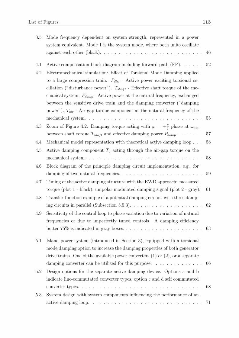
List of Figures 113
3.5 Mode frequency dependent on system strength, represented in a power
system equivalent. Mode 1 is the system mode, where both units oscillate
against each other (black). . . . . . . . . . . . . . . . . . . . . . . . . . . . 46
4.1 Active compensation block diagram including forward path (FP). . . . . . 52
4.2 Electromechanical simulation: Effect of Torsional Mode Damping applied
to a large compression train. Pdist - Active power exciting torsional os-
cillation (”disturbance power”). Tshaft - Effective shaft torque of the me-
chanical system. Pdamp - Active power at the natural frequency, exchanged
between the sensitive drive train and the damping converter (”damping
power”). Tair - Air-gap torque component at the natural frequency of the
mechanical system. . . . . . . . . . . . . . . . . . . . . . . . . . . . . . . . 55
4.3 Zoom of Figure 4.2: Damping torque acting with ϕ = +π2
phase at ωnat
between shaft torque Tshaft and effective damping power Pdamp. . . . . . . 57
4.4 Mechanical model representation with theoretical active damping loop . . . 58
4.5 Active damping component Td acting through the air-gap torque on the
mechanical system. . . . . . . . . . . . . . . . . . . . . . . . . . . . . . . . 58
4.6 Block diagram of the principle damping circuit implementation, e.g. for
damping of two natural frequencies. . . . . . . . . . . . . . . . . . . . . . . 59
4.7 Tuning of the active damping structure with the EWD approach: measured
torque (plot 1 - black), unipolar modulated damping signal (plot 2 - gray). 61
4.8 Transfer-function example of a potential damping circuit, with three damp-
ing circuits in parallel (Subsection 5.5.3). . . . . . . . . . . . . . . . . . . . 62
4.9 Sensitivity of the control loop to phase variation due to variation of natural
frequencies or due to imperfectly tuned controls. A damping efficiency
better 75% is indicated in gray boxes. . . . . . . . . . . . . . . . . . . . . . 63
5.1 Island power system (introduced in Section 3), equipped with a torsional
mode damping option to increase the damping properties of both generator
drive trains. One of the available power converters (1) or (2), or a separate
damping converter can be utilized for this purpose. . . . . . . . . . . . . . 66
5.2 Design options for the separate active damping device. Options a and b
indicate line-commutated converter types, option c and d self commutated
converter types. . . . . . . . . . . . . . . . . . . . . . . . . . . . . . . . . . 68
5.3 System design with system components influencing the performance of an
active damping loop. . . . . . . . . . . . . . . . . . . . . . . . . . . . . . . 71
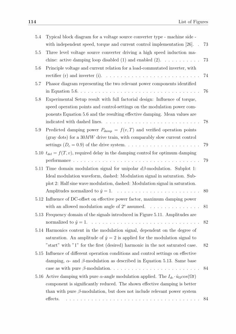
114 List of Figures
5.4 Typical block diagram for a voltage source converter type - machine side -
with independent speed, torque and current control implementation [26]. . 73
5.5 Three level voltage source converter driving a high speed induction ma-
chine: active damping loop disabled (1) and enabled (2). . . . . . . . . . . 73
5.6 Principle voltage and current relation for a load-commutated inverter, with
rectifier (r) and inverter (i). . . . . . . . . . . . . . . . . . . . . . . . . . . 74
5.7 Phasor diagram representing the two relevant power components identified
in Equation 5.6. . . . . . . . . . . . . . . . . . . . . . . . . . . . . . . . . . 76
5.8 Experimental Setup result with full factorial design: Influence of torque,
speed operation points and control-settings on the modulation power com-
ponents Equation 5.6 and the resulting effective damping. Mean values are
indicated with dashed lines. . . . . . . . . . . . . . . . . . . . . . . . . . . 78
5.9 Predicted damping power Pdamp = f(v, T ) and verified operation points
(gray dots) for a 30MW drive train, with comparably slow current control
settings (Dc = 0.9) of the drive system. . . . . . . . . . . . . . . . . . . . . 79
5.10 tdel = f(T, v), required delay in the damping control for optimum damping
performance . . . . . . . . . . . . . . . . . . . . . . . . . . . . . . . . . . . 79
5.11 Time domain modulation signal for unipolar dβ-modulation. Subplot 1:
Ideal modulation waveform, dashed: Modulation signal in saturation. Sub-
plot 2: Half sine wave modulation, dashed: Modulation signal in saturation.
Amplitudes normalized to y = 1. . . . . . . . . . . . . . . . . . . . . . . . 80
5.12 Influence of DC-offset on effective power factor, maximum damping power
with an allowed modulation angle of 2o assumed. . . . . . . . . . . . . . . 81
5.13 Frequency domain of the signals introduced in Figure 5.11. Amplitudes are
normalized to y = 1. . . . . . . . . . . . . . . . . . . . . . . . . . . . . . . 82
5.14 Harmonics content in the modulation signal, dependent on the degree of
saturation. An amplitude of y = 2 is applied for the modulation signal to
”start” with ”1” for the first (desired) harmonic in the not saturated case. 82
5.15 Influence of different operation conditions and control settings on effective
damping, α- and β-modulation as described in Equation 5.13. Same base
case as with pure β-modulation. . . . . . . . . . . . . . . . . . . . . . . . . 84
5.16 Active damping with pure α-angle modulation applied. The Idc · uΩcos(Ωt)
component is significantly reduced. The shown effective damping is better
than with pure β-modulation, but does not include relevant power system
effects. . . . . . . . . . . . . . . . . . . . . . . . . . . . . . . . . . . . . . 84
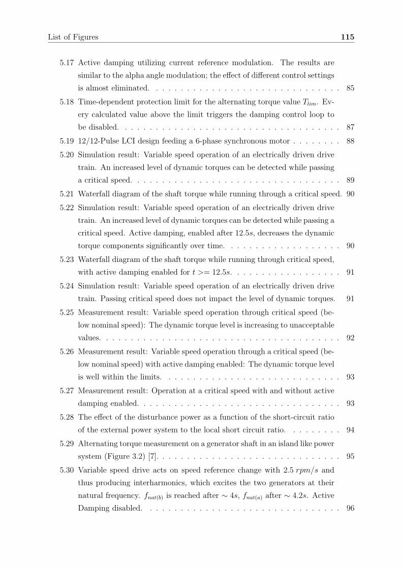
List of Figures 115
5.17 Active damping utilizing current reference modulation. The results are
similar to the alpha angle modulation; the effect of different control settings
is almost eliminated. . . . . . . . . . . . . . . . . . . . . . . . . . . . . . . 85
5.18 Time-dependent protection limit for the alternating torque value Tlim. Ev-
ery calculated value above the limit triggers the damping control loop to
be disabled. . . . . . . . . . . . . . . . . . . . . . . . . . . . . . . . . . . . 87
5.19 12/12-Pulse LCI design feeding a 6-phase synchronous motor . . . . . . . . 88
5.20 Simulation result: Variable speed operation of an electrically driven drive
train. An increased level of dynamic torques can be detected while passing
a critical speed. . . . . . . . . . . . . . . . . . . . . . . . . . . . . . . . . . 89
5.21 Waterfall diagram of the shaft torque while running through a critical speed. 90
5.22 Simulation result: Variable speed operation of an electrically driven drive
train. An increased level of dynamic torques can be detected while passing a
critical speed. Active damping, enabled after 12.5s, decreases the dynamic
torque components significantly over time. . . . . . . . . . . . . . . . . . . 90
5.23 Waterfall diagram of the shaft torque while running through critical speed,
with active damping enabled for t >= 12.5s. . . . . . . . . . . . . . . . . . 91
5.24 Simulation result: Variable speed operation of an electrically driven drive
train. Passing critical speed does not impact the level of dynamic torques. 91
5.25 Measurement result: Variable speed operation through critical speed (be-
low nominal speed): The dynamic torque level is increasing to unacceptable
values. . . . . . . . . . . . . . . . . . . . . . . . . . . . . . . . . . . . . . . 92
5.26 Measurement result: Variable speed operation through a critical speed (be-
low nominal speed) with active damping enabled: The dynamic torque level
is well within the limits. . . . . . . . . . . . . . . . . . . . . . . . . . . . . 93
5.27 Measurement result: Operation at a critical speed with and without active
damping enabled. . . . . . . . . . . . . . . . . . . . . . . . . . . . . . . . . 93
5.28 The effect of the disturbance power as a function of the short-circuit ratio
of the external power system to the local short circuit ratio. . . . . . . . . 94
5.29 Alternating torque measurement on a generator shaft in an island like power
system (Figure 3.2) [7]. . . . . . . . . . . . . . . . . . . . . . . . . . . . . . 95
5.30 Variable speed drive acts on speed reference change with 2.5 rpm/s and
thus producing interharmonics, which excites the two generators at their
natural frequency. fnat(b) is reached after ∼ 4s, fnat(a) after ∼ 4.2s. Active
Damping disabled. . . . . . . . . . . . . . . . . . . . . . . . . . . . . . . . 96
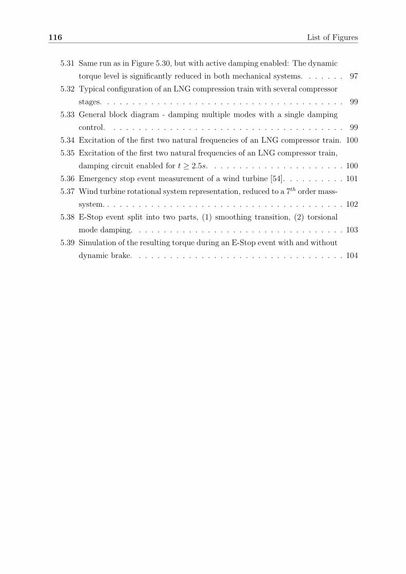
116 List of Figures
5.31 Same run as in Figure 5.30, but with active damping enabled: The dynamic
torque level is significantly reduced in both mechanical systems. . . . . . . 97
5.32 Typical configuration of an LNG compression train with several compressor
stages. . . . . . . . . . . . . . . . . . . . . . . . . . . . . . . . . . . . . . . 99
5.33 General block diagram - damping multiple modes with a single damping
control. . . . . . . . . . . . . . . . . . . . . . . . . . . . . . . . . . . . . . 99
5.34 Excitation of the first two natural frequencies of an LNG compressor train. 100
5.35 Excitation of the first two natural frequencies of an LNG compressor train,
damping circuit enabled for t ≥ 2.5s. . . . . . . . . . . . . . . . . . . . . . 100
5.36 Emergency stop event measurement of a wind turbine [54]. . . . . . . . . . 101
5.37 Wind turbine rotational system representation, reduced to a 7th order mass-
system. . . . . . . . . . . . . . . . . . . . . . . . . . . . . . . . . . . . . . . 102
5.38 E-Stop event split into two parts, (1) smoothing transition, (2) torsional
mode damping. . . . . . . . . . . . . . . . . . . . . . . . . . . . . . . . . . 103
5.39 Simulation of the resulting torque during an E-Stop event with and without
dynamic brake. . . . . . . . . . . . . . . . . . . . . . . . . . . . . . . . . . 104
Bibliography
[1] A. T. D. Almeida, F. J. T. E. Ferreira, and P. Fonseca, “VSDs for Electric Motor
Systems,” 2000.
[2] V. Hutten, R. M. Zurowski, and M. Hilscher, “Torsional Interharmonic Interaction
Study of 75MW Direct Driven VSDS Motor Compressor Train for LNG Duty,”
No. 37, (Turbomachinery Laboratory, Texas A&M University, College Station,
Texas), Turbomachinery Symposium, 2008.
[3] T. Feese and R. Maxfiedl, “Torsional Vibration Problem with Motor/ID Fan Sys-
tem Due to PWM Variable Frequency Drive,” No. 37, (Turbomachinery Laboratory,
Texas A&M University, College Station, Texas), Turbomachinery Symposium, 2008.
[4] K. T. Andersen, “Torsional Oscillation in Drive Systems,” 2005.
[5] F. Joswig and S. Kulig, “Perception about new kinds of subsynchronous resonances,”
(Rio de Janeiro), IPST, 2001.
[6] P. Kundur, Power System Stability and Control. No. 978-0070359581, New York:
McGraw-Hill, 1994.
[7] M. Hernes, “Risk for interaction between components in power grids containing a
high percentage of converter loads,” 2002.
[8] “API Standard 617 - Axial and Centrifugal Compressors and Expander-Compressors
for Petroleum, Chemical and Gas Industry Services,” 2002.
[9] H. Dresig and F. Holzweißig, Maschinendynamik. No. 978-3540876939 in 7, Berlin:
Springer Verlag, 2006.
[10] J. Huster and A. Ziegler, “Simulation der Beanspruchungen der Wellen und lan-
gen Niederdruck Schaufeln grosser Dampfturbinensatze mit geschweissten ND-
Trommelrotoren in thermischen Kraftwerken bei elektrischen Stoerfallen,” vol. 1749,
2003.
117
118 Bibliography
[11] M. A. Corbo, “Torsional Vibration Analysis of Synchronous Motor-Driven Turbo-
machinery,” No. 29, (Turbomachinery Laboratory, Texas A&M University, College
Station, Texas), Turbomachinery Symposium, 2000.
[12] C. Sihler, “A novel torsional exciter for modal vibration testing of large rotating
machinery,” vol. 20, pp. 1725–1740, Mechanical Systems and Signal Processing, 2006.
[13] C. Sihler, S. Schramm, J. Song-Manguelle, P. Rotondo, S. D. Puglia, and E. Larsen,
“Torsional Mode Damping For Electrically Driven Gas Compression Trains In Ex-
tended Variable Speed Operation,” No. 38, (Turbomachinery Laboratory, Texas
A&M University, College Station, Texas), pp. 81–92, Turbomachinery Symposium,
2009.
[14] H. Holzer, Die Berechnung der Drehschwingungen. No. 978-1161070880, Berlin:
Springer Verlag, 1912.
[15] E. I. Rivin, “Methode zur Verminderung der Freiheitsgrade in Berechungsmodellen
verketteter und verzweigter Systeme,” pp. 38–41, Vestnik Masinostronenija, 1966.
[16] P. N. Di, Beitrag zur Reduktion diskreter Schwingunsketten auf ein Minimalmodell.
PhD thesis, TU Dresden, 1973.
[17] M. Bressani, A. Odorico, and M. Sica, “High-Speed, Large-Power Induction Mo-
tors for Direct Coupling to Variable Speed Gas Compressors,” vol. Fifth European
Conference on Power Electronics and Applications, 1993.
[18] W. Wenzke, “Zur Ableitung der dynamischen Kennlinie des Asynchronmotors im
Hinblick auf die Berechnung von Schwingungserscheinungen in Antriebsanlagen,”
pp. 517–523, Wiss. Zeitschrift der TU Magdeburg, 1970.
[19] C. M. Ong, Dynamic Simulation of Electric Machinery using Matlab/ Simulink.
No. 978-0137237852, Prentice Hall, 1999.
[20] T. Bodefeld, Elektrische Maschinen. No. B0000BGNS8, Springer Verlag, 1949.
[21] B. K. Bose, Power Electronics and Motor Drives Advances and Trends. No. 978-
0120884056, Academic Press, 2006.
[22] N. G. Hingorani and L. Gyugyi, Understanding Facts. No. 978-0780334557, IEEE
press, 2000.

Bibliography 119
[23] E. Morris, “A Guide to Standard Medium Voltage Variable Speed Drives,” ABB
Industrie AG, 2008.
[24] R. Klug and A. Mertens, “Reliability of Megawatt Drive Concepts,” vol. 2, pp. 636–
641, IEEE International Conference on Industrial Technology, 2003.
[25] A. Siebert, A. Troedson, and S. Ebner, “AC to DC Power Conversion Now and in
the Future,” vol. 38, IEEE Transactions on Industry Applications, 2002.
[26] W. Leonhard, Control of Electrical Drives. No. 978-3540418207, Berlin: Springer
Verlag, 1997.
[27] J. J. Simond, A. Sapin, M. T. Xuan, R. Wetter, and P. Burmeister, “12-Pulse LCI
Synchronous Drive for a 20 MW Compressor - Modeling, Simulation and Measure-
ments,” pp. 2302–2308, IEEE Transactions On Industry Applications, 2005.
[28] A. Adachi, K. Tanaka, and Y. Fukushima, “Torsional Lateral Coupled Vibration
of Centrifugal Compressor System at Interharmonic Frequencies Related to Control
Loop Frequencies in Voltage Source PWM Inverter,” No. 38, (Turbomachinery Labo-
ratory, Texas A&M University, College Station, Texas), Turbomachinery Symposium,
2009.
[29] P. M. Anderson, B. L. Agrawal, and J. E. V. Ness, Subsynchronous Resonance in
Power Systems. No. 978-0780353503, Technology & Engineering, 1999.
[30] S. Kulig and D. Lambrecht, “Resonant Excitation of Turbine Generator Shaft,”
(Stuttgart), The Road-Vehicle-System and Related Mathematics Workshop, 1985.
[31] S. Kulig, Uber die Auswirkungen von Storfallen in elektrischen Energieubertra-
gungsnetzen auf Kraftwerksturbosatze. PhD thesis, FU Hagen, 1987.
[32] M. Humer, Erfassung und Bewertung von Torsionsschwingungen in Wellenstrangen
von Kraftwerksturbosatzen. PhD thesis, Universitat Dortmund, 2004.
[33] D. Lee and P. Kundur, “Advanced Excitation Controls for Power System Stability
Enhancement,” vol. 38-01, (Paris), CIGRE, 1986.
[34] “Std 1204-1997 - Guide for Planning DC Links Terminating at AC Locations Having
Low Short-Circuit Capacities, PartI: AC/DC Interaction Phenomena,” 1997.
120 Bibliography
[35] K. Mortensen, E. V. Larsen, and R. J. Piwko, “Field Tests and Analysis of Torsional
Interaction Between the Coal Creek Turbine-Generators and the CU HVDC System,”
IEEE transaction on power apparatus and systems, 1981.
[36] R. J. Piwko and E. V. Larsen, “HVDC System Control For Damping Subsynchronous
Oscillation,” vol. PAS-101, IEEE transaction on power apparatus and systems, 1982.
[37] A. Abedini, G. Mandic, and A. Nasiri, “Wind power smoothing using rotor inertia
aimed at reducing grid susceptibility,” No. 34th, pp. 1445–1451, 2008,.
[38] T. Feese and C. Hill, “Prevention of Torsional Vibration Problems in Reciprocating
Machinery,” No. 38, (Turbomachinery Laboratory, Texas A&M University, College
Station, Texas), pp. 213–239, Turbomachinery Symposium, 2009.
[39] H. Muller, M. Poller, A. Basteck, M. Tilscher, and J. Pfister, “Grid Compatibil-
ity of Variable Speed Wind Turbines with Directly Coupled Synchronous Generator
and Hydro-Dynamically Controlled Gearbox,” vol. 6, (Delft, NL), Workshop on In-
ternational Large Scale Integration of Wind Power and Transmission Networks for
Offshore Wind Farms, 2006.
[40] D. E. Walker, C. Bowler, R. Jackson, and D. Hodges, “Results of SSR Tests at
Mohave,” vol. PAS-94, pp. 1878–1889, IEEE Transactions, 1975.
[41] M. Perrin, G. Kohn, S. Mugford, and G. Seggewiss, “Induction motors, reciprocating
compressors and variable frequency drives,” vol. 44, (Banff, Alta.), The Institute of
Electrical and Electronics Engineers Incorporated Industry Applications Society -
Petroleum and Chemical Industry Conference, 1997.
[42] GEEnergy, Turbine-Generator Torsional Stress Analyzer (TSA).
http://www.gepower.com/.../downloads/10088.pdf, 2004.
[43] “Countermeasures to Subsynchronous Resonance Problems,” 1980.
[44] N. Olgac, “Delayed Resonator as active absorber,” 1995.
[45] D. Schroder, Elektrische Antriebe-Regelung von Antriebssystemen. No. 978-
3540419945, Springer Verlag, 2001.
[46] T. Kakinoki, R. Yokoyama, G. Fujita, K. Koyanagi, and T. Funabashi, “Evaluation
technique of turbine shaft fatigue in private-generation systems using consumption
rate of shaft life cycle,” pp. 779–783, IEEE International Conference on Power System
Technology, 2002.
Bibliography 121
[47] E. V. Larsen, “Applying Power System Stabilizers, Part I-III,” vol. PAS-100, IEEE
Transaction on Power Apparatus and Systems, 1981.
[48] R. J. Piwko, C. A. Wegner, S. J. Kinney, and J. D. Eden, “Subsynchronous Reso-
nance Performance Tests of the Slatt Thyristor-Controlled Series Capacitor,” vol. 11,
pp. 1112–1119, IEEE Transactions on Power Delivery, 1996.
[49] A. Wirsen and S. Kulig, “A Contact-Less Torque Sensor for Online Monitoring of
Torsional Oscillations,” 2007.
[50] C. Sihler and A. M. Miri, “A Stabilizer for Oscillating Torques in Synchronous Ma-
chines,” vol. 41, IEEE Transaction on Industry Applications, 2005.
[51] T. Zoller, A. M. Miri, and T. Leibfried, “Power Electronic Devices for Damping
Torsional Vibrations,” No. 7, International Conference on Power Electronics and
Drive Systems, 2007.
[52] S. Schramm, “Torsional Mode Damping in Island Power Systems,” Master’s thesis,
Munich University of Applied Sciences, 2006.
[53] S. Schramm, C. Sihler, J. Song-Manguelle, and P. Rotondo, “Damping Torsional
Interaction Effects of Large Drives,” vol. 25, pp. 1090–1098, IEEE Transactions on
Power Electronics, 2010.
[54] J. Hemmelmann, “Latest Results On Transmission and Conversion,” (Brussels),
2008.
[55] A. Heege, “Computation of Dynamic Loads of Wind Turbine Power Trains,”
vol. XXVI, (Cordoba, Argentina), pp. 2985–3004, Mecanica Computational, 2007.
[56] “CompactRIO-PAC-Hardware,” (www.ni.com/pac/d/crio.htm), National Instru-
ments, 2009.
