declarative datalog debugging for mere mortals · pdf filedeclarative datalog debugging for...
TRANSCRIPT
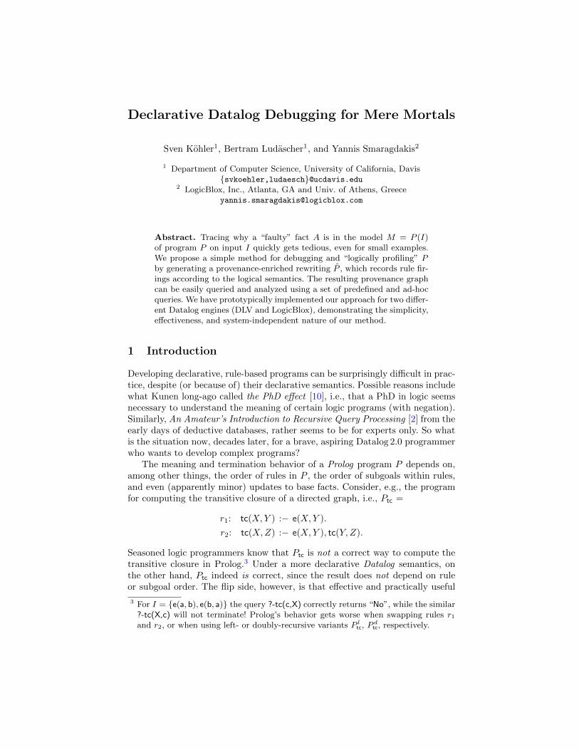
Declarative Datalog Debugging for Mere Mortals
Sven Kohler1, Bertram Ludascher1, and Yannis Smaragdakis2
1 Department of Computer Science, University of California, Davis{svkoehler,ludaesch}@ucdavis.edu
2 LogicBlox, Inc., Atlanta, GA and Univ. of Athens, [email protected]
Abstract. Tracing why a “faulty” fact A is in the model M = P (I)of program P on input I quickly gets tedious, even for small examples.We propose a simple method for debugging and “logically profiling” Pby generating a provenance-enriched rewriting P , which records rule fir-ings according to the logical semantics. The resulting provenance graphcan be easily queried and analyzed using a set of predefined and ad-hocqueries. We have prototypically implemented our approach for two differ-ent Datalog engines (DLV and LogicBlox), demonstrating the simplicity,effectiveness, and system-independent nature of our method.
1 Introduction
Developing declarative, rule-based programs can be surprisingly difficult in prac-tice, despite (or because of) their declarative semantics. Possible reasons includewhat Kunen long-ago called the PhD effect [10], i.e., that a PhD in logic seemsnecessary to understand the meaning of certain logic programs (with negation).Similarly, An Amateur’s Introduction to Recursive Query Processing [2] from theearly days of deductive databases, rather seems to be for experts only. So whatis the situation now, decades later, for a brave, aspiring Datalog 2.0 programmerwho wants to develop complex programs?
The meaning and termination behavior of a Prolog program P depends on,among other things, the order of rules in P , the order of subgoals within rules,and even (apparently minor) updates to base facts. Consider, e.g., the programfor computing the transitive closure of a directed graph, i.e., Ptc =
r1: tc(X,Y ) :− e(X,Y ).
r2: tc(X,Z) :− e(X,Y ), tc(Y,Z).
Seasoned logic programmers know that Ptc is not a correct way to compute thetransitive closure in Prolog.3 Under a more declarative Datalog semantics, onthe other hand, Ptc indeed is correct, since the result does not depend on ruleor subgoal order. The flip side, however, is that effective and practically useful
3 For I = {e(a, b), e(b, a)} the query ?-tc(c,X) correctly returns “No”, while the similar?-tc(X,c) will not terminate! Prolog’s behavior gets worse when swapping rules r1and r2, or when using left- or doubly-recursive variants P l
tc, Pdtc, respectively.
procedural debugging techniques for Prolog, based on the box model [19], arenot available in Datalog. Instead, new debugging techniques are needed that aresolely based on the declarative reading of rules. In this paper, we develop sucha framework for declarative debugging and logic profiling.
Let M=P (I) be the model of P on input I. Bugs in P (or I) manifestthemselves through unexpected answers (ground atoms) A ∈M , or expected butmissing A /∈M . The key idea of our approach is to rewrite P into a provenance-enriched program P , which records the derivation history of M=P (I) in anextended model M=P (I). A provenance graph G is then extracted from M ,which the user can explore further via predefined views and ad-hoc queries.
Use Cases Overview. Given an IDB atom A, our approach allows to answerquestions such as the following: What is the data lineage of A, i.e., the set ofEDB facts that were used in a derivation of A, and what is the rule lineage, i.e.,the set of rules used to derive A? When chasing a bug or trying to locate a sourceof inefficiency, a user can explore further details: What is the graph structureGA of all derivations of A? What is the length of A, i.e., of shortest derivations,and what is the weight, i.e., number of simple derivations (proof trees) of A?
For another example, assume the user encounters two “suspicous” atoms Aand B. It is easy to compute the common lineage GAB = GA ∩ GB sharedby A and B, or the lowest common ancestors of A and B, i.e., the rule firingsand ground atoms that occur “closest” to A and B in GAB , thus triangulatingpossible sources of error, somewhat similar to ideas used in delta debugging [22].
Since nodes in GA are associated with relation symbols and rules, a usermight also want to compute other aggregates, i.e., not only at the level of GA
(ground atoms and firings), but at the level of (non-ground) rules and relationsymbols, respectively. Through this schema-level profiling, a user can quickly findthe hot (cold) spots in P , e.g., rules having the most (least) number of firings.
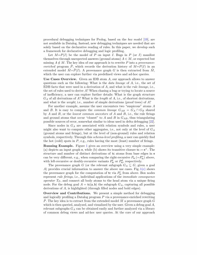
Running Example. Figure 1 gives an overview using a very simple example:(a) depicts an input graph e, while (b) shows its transitive closure tc := e+. Thestructure and number of distinct derivations of tc atoms from base edges in ecan be very different, e.g., when comparing the right-recursive Ptc (=P r
tc) above,with left-recursive or doubly-recursive variants P l
tc or P dtc, respectively.
The provenance graph G (or the relevant subgraph GA ⊆ G, given a goalA) provides crucial information to answer the above use cases. Fig. 1(c) showsthe provenance graph for the computation of tc via P r
tc from above. Box nodesrepresent rule firings, i.e., individual applications of the immediate consequenceoperator TP , and connect all body atoms to the head atom via a unique firingnode. For the debug goal A = tc(a, b) the subgraph GA, capturing all possiblederivations of A, is highlighted (through filled nodes and bold edges).
Overview and Contributions. We present a simple method for debuggingand logically profiling a Datalog program P via a provenance-enriched rewritingP . The key idea is to extract from the extended model M a provenance graph Gwhich is then queried, analyzed, and visualized by the user. Given a debug goal A,relevant subgraphs GA can be obtained easily and further analyzed via a libraryof common debug views and ad-hoc user queries. At the core of our approach
a b c d(a) Input graph: edge relation e
a bc
d
(b) Output: transitive closure tc = e+
e(a,b)
r1
r2
r2
r2
tc(a,b)
tc(a,c)
tc(a,d)
e(b,c) r1
r2
r2
r2
tc(b,c)
tc(b,b)
tc(b,d)
e(c,b)
r1
r2
r2
r2
tc(c,b)
tc(c,c)
tc(c,d)e(c,d) r1
(c) Provenance graph G; highlighted subgraph Gtc(a,b); firing nodes r (boxes),
atom nodes A (ovals); edge types Ain→ r and r
out_A (edge labels not shown)
Fig. 1. P rtc-provenance graph for input e, with derivations of tc(a,b) highlighted in (c).
are rewritings that (i) capture rule firings, then (ii) reify them, i.e., turn theminto nodes in G (via Skolem functions), while (iii) keeping track of derivationlengths using Statelog [11], a Datalog variant with states.4 The rewritten Statelogprogram P is state-stratified [13] and has ptime data complexity. We view thesimplicity and system-independence as an important benefit of our approach. Wehave rapidly prototyped this approach for rather different Datalog engines, i.e.,DLV [12] and LogicBlox [14], and are currently developing improved versions.We also note a close relationship of our provenance graphs with provenancesemirings [8] (a detailed account is beyond the scope of this paper). Here ourfocus is on presenting a simple, effective method for debugging and profilingdeclarative rules for “mere mortals”.
2 Provenance Rewritings for Datalog
In this section, we present three Datalog rewritings PF · G · S P for capturing
rule firings, graph generation, and Statelog evaluation, respectively. We assumethe reader is familiar with Datalog (e.g., see [1, 17]); the resulting Statelogprogram P has ptime data complexity and involves a limited (i.e., safe) form ofSkolem functions and state terms [13]. In the sequel, X = X1, . . . , Xn denotes avariable vector; lower case terms a, b, . . . denote constants.
4 Other state-oriented Datalog extensions include DatalognS [6] and XY-Datalog [21].
e(a,b)fire1(a,b)(*)
fire2(a,b,b)
(*) tc(a,b)(+)
(+)
tc(b,b)
(*)
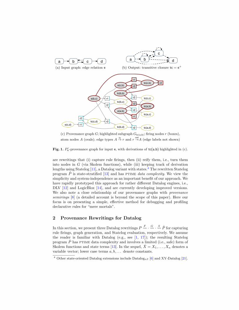
Fig. 2. Subgraph with two rule firings fire1(a, b) and fire2(a, b, b), both deriving tc(a,b).
2.1 Recording Rule Firings: PF P F
The first rewriting (cf. Green et al. [9]), captures the provenance of rule firings.Let r be a unique identifier of a rule in P . We assume r to be safe, i.e., everyvariable in r must also occur positively in the body:
r : H(Y ) :− B1(X1), . . . , Bn(Xn)
Let X :=⋃
i Xi include all variables in r, ordered, e.g., by occurrence in the body.Since r is safe, Y ⊆ X, i.e., the head variables are among the X. The rule r isnow replaced by two new rules in the rewritten program PF :
rin : firer(X) :− B1(X1), . . . , Bn(Xn)
rout : H(Y ) :− firer(X)
Thus PF records, for each r-satisfying instance x of X, a unique fact: firer(x).
2.2 Graph Reification of Firings: P F G PG
To facilitate querying the results of the previous step, we reify ground atoms andfirings as nodes in a labeled provenance graph G. For each pair of rules rin, routabove, we add n rules (i = 1, . . ., n) to generate the in-labeled edges in G:
g( Bi(Xi), in, firer(X) ) :− firer(X)
and one more rule for generating out-labeled edges in G as well:
g( firer(X), out, H(Y ) ) :− firer(X)
Note the safe use of atoms as Skolem terms in the rule heads: for finitely manyrule firings firer(x), we obtain a finite number of in- and out-edges in G.
Example. After applying both transformations · F · G · to Ptc from above, the
rewritten program PGtc can be executed, yielding a directed graph with labeled
edges g(v1, `, v2) in the enriched model M . Figure 2 shows a subgraph with tworule firings, both deriving the atom tc(a,b). Oval (yellow) nodes represent atomsA and boxed (blue) nodes represent firings F . Arrows with solid heads and label(*) are in-edges, while those with empty heads and label (+), represent out-edges. Note that according to the declarative semantics, in (out) edges, modellogical conjunction “∧” (logical disjunction “∨”), respectively. Thus, w.r.t. theirincoming edges, boxed nodes are AND-nodes, while oval nodes are OR-nodes.5
5 In semiring parlance, they are product “⊗” and sum “⊕” nodes, respectively.
2.3 Statelog Rewriting: PG S PS
Statelog [11, 13] is a state-oriented Datalog variant for expressing active updaterules and declarative rules in a unified framework. The next rewriting simulatesa Statelog derivation in Datalog via a limited (safe) form of “state-generation”.The key idea is to keep track of the firing rounds In+1 := TP (In) of the TP
operator (I0 := I is the input database). This provides a simple yet powerfulmeans to detect tuple rederivations, to identify unfounded derivations, etc.
First, replace all rules rin, rout above with their state-oriented counterparts:
rin : firer(S1, X) :− B1(S, X1), . . . , Bn(S, Xn), next(S,S1).
rout : H(S, Y ) :− firer(S, X).
The goal next(S,S1) is used for the safe generation of new states: The next states+1 is generated only if at least one atom A was new in state s :
next(0, 1) :− true.
next(S,S1) :− next( ,S), new(S, A), S1 := S + 1.
An atom A is newly derived if it is true in s+1, but not in the previous state s:
newAtom(S1, A) :− next(S,S1), g(S1, , out, A), ¬ g(S, , out, A).
Similarly, rule firing F is new if it is true in s+1, but not previously in s:
newFiring(S1, F ) :− next(S,S1), g(S1, F, out, ), ¬ g(S, F, out, ).
The n rules for generating in-edges are replaced with state-oriented versions:
g( S, Bi(Xi), in, firer(X) ) :− firer(S, X)
and similarly, for the out-edge generating rules:
g( S, firer(X), out, H(Y ) ) :− firer(S, X).
It is not difficult to see that the above rules are state-stratified (a form of lo-cal stratification) and that the resulting program terminates after polynomiallymany steps [13]: When no more new atoms (or firings) are derived in a state,then the above rules for next can no longer generate new states, thus in turnpreventing rules of type rin from generating new firer(S1, X) atoms.
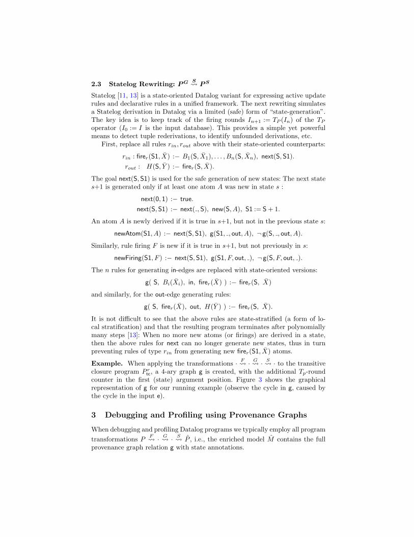
Example. When applying the transformations · F · G · S · to the transitive
closure program P rtc, a 4-ary graph g is created, with the additional Tp-round
counter in the first (state) argument position. Figure 3 shows the graphicalrepresentation of g for our running example (observe the cycle in g, caused bythe cycle in the input e).
3 Debugging and Profiling using Provenance Graphs
When debugging and profiling Datalog programs we typically employ all program
transformations PF · G
· S P , i.e., the enriched model M contains the full
provenance graph relation g with state annotations.
e(a,b) r1 [1]
r2 [3]
tc(a,b)[1]e(b,c)
r2 [2] tc(b,b)[2]
e(c,b)r1 [1]
r2 [3]
tc(c,b)[1]
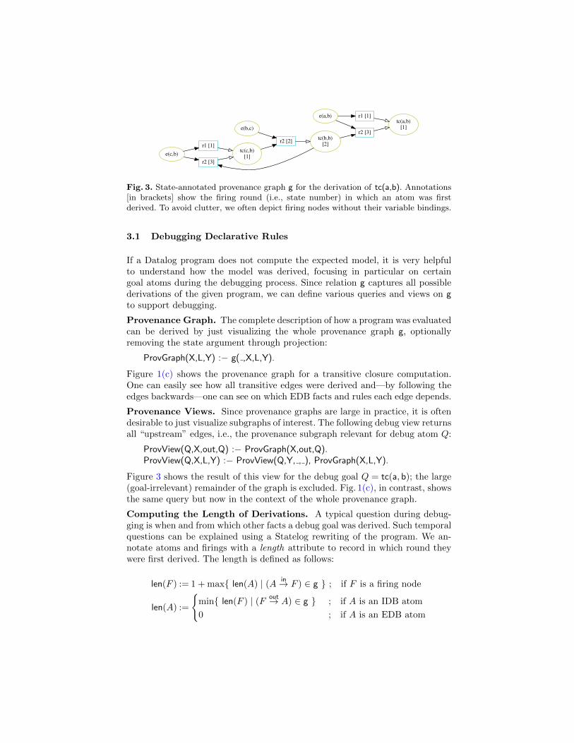
Fig. 3. State-annotated provenance graph g for the derivation of tc(a,b). Annotations[in brackets] show the firing round (i.e., state number) in which an atom was firstderived. To avoid clutter, we often depict firing nodes without their variable bindings.
3.1 Debugging Declarative Rules
If a Datalog program does not compute the expected model, it is very helpfulto understand how the model was derived, focusing in particular on certaingoal atoms during the debugging process. Since relation g captures all possiblederivations of the given program, we can define various queries and views on gto support debugging.
Provenance Graph. The complete description of how a program was evaluatedcan be derived by just visualizing the whole provenance graph g, optionallyremoving the state argument through projection:
ProvGraph(X,L,Y) :− g( ,X,L,Y).
Figure 1(c) shows the provenance graph for a transitive closure computation.One can easily see how all transitive edges were derived and—by following theedges backwards—one can see on which EDB facts and rules each edge depends.
Provenance Views. Since provenance graphs are large in practice, it is oftendesirable to just visualize subgraphs of interest. The following debug view returnsall “upstream” edges, i.e., the provenance subgraph relevant for debug atom Q:
ProvView(Q,X,out,Q) :− ProvGraph(X,out,Q).ProvView(Q,X,L,Y) :− ProvView(Q,Y, , ), ProvGraph(X,L,Y).
Figure 3 shows the result of this view for the debug goal Q = tc(a, b); the large(goal-irrelevant) remainder of the graph is excluded. Fig. 1(c), in contrast, showsthe same query but now in the context of the whole provenance graph.
Computing the Length of Derivations. A typical question during debug-ging is when and from which other facts a debug goal was derived. Such temporalquestions can be explained using a Statelog rewriting of the program. We an-notate atoms and firings with a length attribute to record in which round theywere first derived. The length is defined as follows:
len(F ) := 1 + max{ len(A) | (A in→ F ) ∈ g } ; if F is a firing node
len(A) :=
{min{ len(F ) | (F out→ A) ∈ g } ; if A is an IDB atom
0 ; if A is an EDB atom
A rule firing F can only succeed one round after the last body atom (i.e., hav-ing maximal length) has been derived. Conversely, the length of an atom A isdetermined by its first derivation (i.e., having minimal length). The Statelogrewriting captures evaluation rounds, so the state associated with a new firingdetermines the length of the firing:
len(F,LenF) :− newFiring(S,F), LenF=S.
Similarly, the length of an atom is equal to the first round it was derived:
len(A,LenA) :− newAtom(S,A), LenA=S.
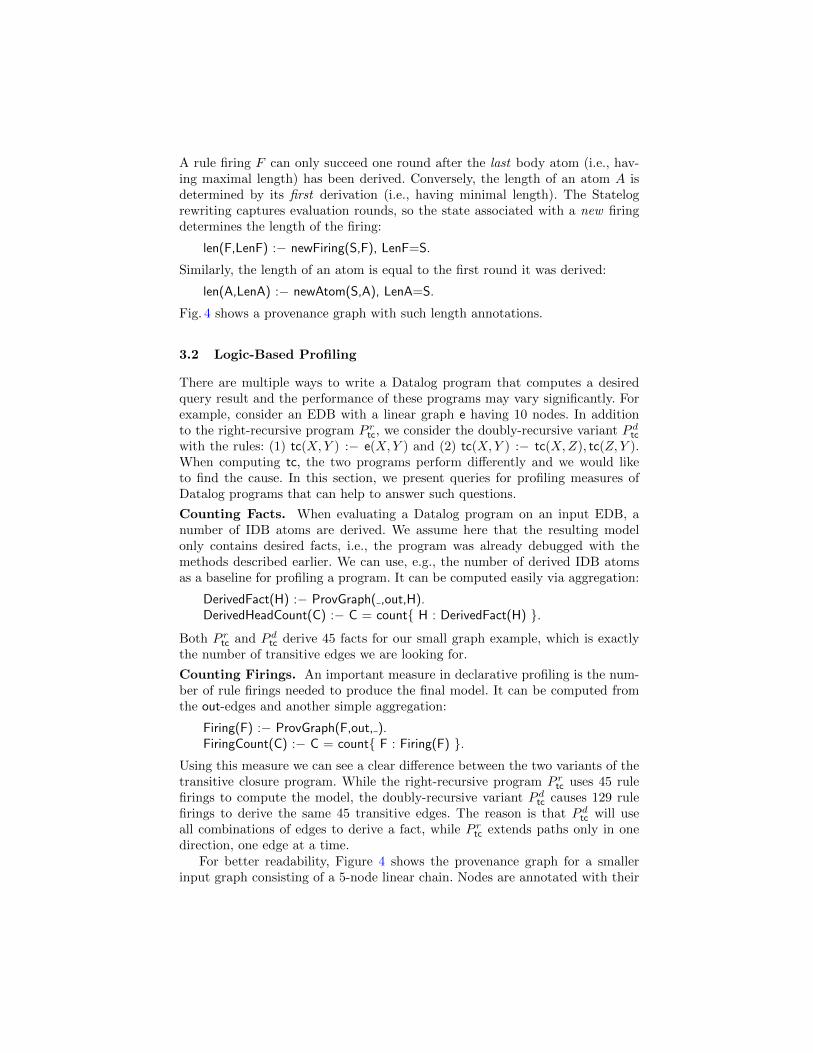
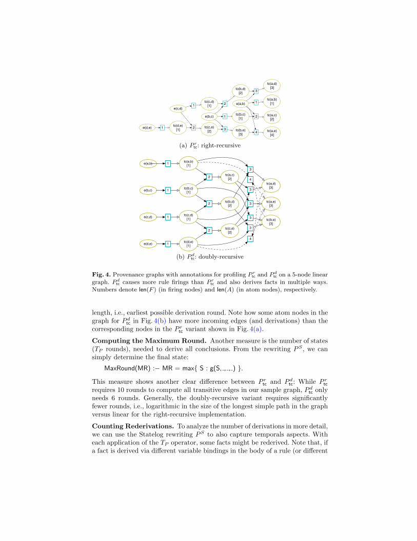
Fig. 4 shows a provenance graph with such length annotations.
3.2 Logic-Based Profiling
There are multiple ways to write a Datalog program that computes a desiredquery result and the performance of these programs may vary significantly. Forexample, consider an EDB with a linear graph e having 10 nodes. In additionto the right-recursive program P r
tc, we consider the doubly-recursive variant P dtc
with the rules: (1) tc(X,Y ) :− e(X,Y ) and (2) tc(X,Y ) :− tc(X,Z), tc(Z, Y ).When computing tc, the two programs perform differently and we would liketo find the cause. In this section, we present queries for profiling measures ofDatalog programs that can help to answer such questions.
Counting Facts. When evaluating a Datalog program on an input EDB, anumber of IDB atoms are derived. We assume here that the resulting modelonly contains desired facts, i.e., the program was already debugged with themethods described earlier. We can use, e.g., the number of derived IDB atomsas a baseline for profiling a program. It can be computed easily via aggregation:
DerivedFact(H) :− ProvGraph( ,out,H).DerivedHeadCount(C) :− C = count{ H : DerivedFact(H) }.
Both P rtc and P d
tc derive 45 facts for our small graph example, which is exactlythe number of transitive edges we are looking for.
Counting Firings. An important measure in declarative profiling is the num-ber of rule firings needed to produce the final model. It can be computed fromthe out-edges and another simple aggregation:
Firing(F) :− ProvGraph(F,out, ).FiringCount(C) :− C = count{ F : Firing(F) }.
Using this measure we can see a clear difference between the two variants of thetransitive closure program. While the right-recursive program P r
tc uses 45 rulefirings to compute the model, the doubly-recursive variant P d
tc causes 129 rulefirings to derive the same 45 transitive edges. The reason is that P d
tc will useall combinations of edges to derive a fact, while P r
tc extends paths only in onedirection, one edge at a time.
For better readability, Figure 4 shows the provenance graph for a smallerinput graph consisting of a 5-node linear chain. Nodes are annotated with their
e(a,b) 1
2
3
4
tc(a,b)[1]
tc(a,c)[2]
tc(a,d)[3]
tc(a,e)[4]
e(b,c) 1
2
3
tc(b,c)[1]
tc(b,d)[2]
tc(b,e)[3]
e(c,d)1
2
tc(c,d)[1]
tc(c,e)[2]
e(d,e) 1 tc(d,e)[1]
(a) P rtc: right-recursive
3
tc(a,d)[3]3
3 tc(a,e)[3]
3 tc(b,e)[3]
3
4
4
e(a,b) 1 tc(a,b)[1]
e(b,c) 1 tc(b,c)[1]
e(c,d) 1 tc(c,d)[1]
e(d,e) 1 tc(d,e)[1]
2
2
2
tc(a,c)[2]
tc(b,d)[2]
tc(c,e)[2]
(b) P dtc: doubly-recursive
Fig. 4. Provenance graphs with annotations for profiling P rtc and P d
tc on a 5-node lineargraph. P d
tc causes more rule firings than P rtc and also derives facts in multiple ways.
Numbers denote len(F ) (in firing nodes) and len(A) (in atom nodes), respectively.
length, i.e., earliest possible derivation round. Note how some atom nodes in thegraph for P d
tc in Fig. 4(b) have more incoming edges (and derivations) than thecorresponding nodes in the P r
tc variant shown in Fig. 4(a).
Computing the Maximum Round. Another measure is the number of states(TP rounds), needed to derive all conclusions. From the rewriting PS , we cansimply determine the final state:
MaxRound(MR) :− MR = max{ S : g(S, , , ) }.
This measure shows another clear difference between P rtc and P d
tc: While P rtc
requires 10 rounds to compute all transitive edges in our sample graph, P dtc only
needs 6 rounds. Generally, the doubly-recursive variant requires significantlyfewer rounds, i.e., logarithmic in the size of the longest simple path in the graphversus linear for the right-recursive implementation.
Counting Rederivations. To analyze the number of derivations in more detail,we can use the Statelog rewriting PS to also capture temporals aspects. Witheach application of the TP operator, some facts might be rederived. Note that, ifa fact is derived via different variable bindings in the body of a rule (or different
rules), the rederivation is captured already in firings. Rederivations occurringduring the fixpoint computation can be captured using the Statelog rewriting:
ReDerivation(S,F) :− g(S,F,out,A), len(A,LenA), LenA < S.ReDerivationCount(S,C) :− C = count{ F : ReDerivation(S,F) }.ReDerivationTotal(T) :− T = sum{ C : ReDerivationCount(S,C) }.
When comparing the rederivation counts, the difference between the Ptc variantsis illuminated further. P r
tc rederives facts 285 times until the fixpoint is reached.The double-recursive program P d
tc causes 325 rederivations.
Schema-Level Profiling. We can easily determine how many new facts perrelation are used in each round to derive new facts:
FactsInRound(S,R,A) :− g(S,A,in, ), RelationName(A,R).FactsInRound(S1,R,A) :− g(S, ,out,A), next(S,S1), RelationName(A,R).NewFacts(S,R,A) :− g(S, ,out,A), ¬FactsInRound(S,R,A), RelationName(A,R).NewFactsCount(S,R,C) :− C = count{ A : NewFacts(S,R,A) }.
This allows us to “plot” the temporal evolution for our result relation R(= tc):For P r
tc and S = 1, . . . , 9 the counts are C = 9, 8, 7, 6, 5, 4, 3, 2, 1, while for P rtc and
S = 1, . . . , 5 we have C = 9, 8, 13, 14, 1. Although P dtc requires fewer rounds than
P rtc, its new fact count mostly increases over time, while for P r
tc, it decreases.
Confronting the Real-World. In practical implementations, the doubly-recursive version P d
tc has horrible performance. For a representative, realisticgraph6 with 1710 nodes and 3936 edges, the right-recursive P r
tc runs in 2.6 sec,while the doubly-recursive P d
tc takes 15.4 sec. Our metrics can easily explainthe discrepancy. The tc-fact count for both versions is 304,000, but the rulefiring count varies widely. Using our program rewriting and the profiling viewFiringCount(C), we discover that P d
tc has over 64 million different rule firings,while P r
tc has under 566 thousand. One reason is that the doubly-recursiverule tc(X,Y ) :− tc(X,Z), tc(Z, Y ) derives the same tc(X,Y ) fact many timesover. This practical example also illustrates the burden of declarative debugging:Adding the profiling calculation to the right-recursive version, P r
tc only growsthe running time slightly, to 3 sec. Adding it to the doubly-recursive P d
tc how-ever, yields a running time of 51.3 sec. This is due to the cost of storing morethan 64 million combinations of variables for rule firings.
4 GPAD Prototype Implementations
By design, our method of provenance-based debugging and profiling only relies onthe declarative reading of rules, i.e., is agnostic about implementation details or
6 The specifics are secondary to our argument, but we list them for completeness. Thegraph is the application-level call-graph and edges indicating whether a method cancall another) for the pmd program from the DaCapo benchmark suite, as producedby a precise low-level program analysis. Timings are on a quad-core Xeon E55302.4GHz 64-bit machine (only one thread was active at a time) with plentiful RAM(24GB) for the analysis, using LogicBlox Datalog ver. 3.7.10.
evaluation techniques specific to the underlying Datalog engine. Indeed, parallelwith the development of the method, we have implemented two incarnations ofa Graph-based Provenance Analyzer and Debugger, i.e., prototypes Gpad/dlvand Gpad/lb, for declarative debugging with the DLV [12] and LogicBlox [14]engines, respectively. Both prototypes “wrap” the underlying Datalog engine,and outsource some processing aspects to a host language.
For example, Gpad/dlv uses Swi-Prolog [20] as a “glue” to automate (1)rule rewritings, (2) invocation of DLV, followed by (3) result post-processing,and (4) result visualization using Graphviz. We are actively developing Gpadfurther and plan a public release in the near future.
5 Related Work
Work on declarative debugging, in particular in the form of algorithmic debugginggoes as far back as the 1980’s [18, 7]. Algorithmic debugging is an interactiveprocess where the user is asked to differentiate between the actual model ofthe (presumeably buggy) program and the user’s intended model. Based on theuser’s input, the system then tries to locate the faulty rules in an interactive ses-sion. Our approach differs in a number of aspects. First, algorithmic debuggingis usually based on a specific operational semantics, i.e., SLDNF resolution, atop-down, left-to-right strategy with backtracking and negation-as-failure, whichdiffers significantly from the declarative Datalog semantics (cf. Section 1). More-over, while our approach is applicable, in principle, in an interactive way, thissuggests a tighter coupling between the debugger and the underlying rule en-gine. In contrast, our approach and its Gpad implementations do not requiresuch tight coupling, but instead treat the rule engine as a black box. In this way,debugging becomes a post-mortem analysis of the provenance-enriched modelM = P (I) via simple yet powerful graph queries and aggregations.
Another approach, more closely related to ours, is the Datalog debugger [3],developed for the DES system. Unlike prior work, and similar to ours, they donot view derivations as SLD proof trees, but rather use a computation graph,similar to our labeled provenance graph. Our approach differs in a number ofways, e.g., our reification of derivations in a labeled graph allows us to use regularpath queries to navigate the provenance graph, locate (least) common ancestorsof buggy atoms, etc. Another difference is our use of Statelog for keeping track ofderivation rounds, which facilitates profiling of the model computation over time(per firing round, identify the rules fired, the number of (re-)derivations per atomor relation, etc.) Recent related work also includes work on trace visualizationfor ASP [4], step-by-step execution of ASP programs [15], and an integrateddebugging environment for DLV [16].
Debugging and Provenance. Chiticariu et al. [5] present a tool for debuggingdatabase schema mappings. They focus on the computation of derivation routesfrom source facts to a target. The method includes the computation of minimalroutes, similar to shortest derivations in our graph. However, their approach
seems less conducive to profiling since, e.g., provenance information on firingrounds is not available in their approach.
There is an intruigingly close relationship between provenance semirings, i.e.,provenance polynomials and formal power series [8], and our labeled provenancegraphs G. The semiring provenance of atom A is represented in the structure ofGA. Consider, e.g., Figure 2: the in-edges of rule firings correspond to a logicalconjunction “∧”, or more abstractly, the product operator “⊗” of the semiring.Similarly, out-edges represent a disjunction “∨”, i.e., an abstract sum operator“⊕”, mirroring the fact that atoms in general have multiple derivations. It is easyto see that a fact A has an infinite number of derivations (proof trees) iff there is acycle in GA: e.g., the derivation of A = tc(a, b) in Figures 1 and 2 involves a cyclethrough tc(b,b), tc(c,b), via two firings of r2. This also explains Prolog’s non-termination (Section 1), which “nicely” mirrors the fact that there are infinitelymany proof trees. On the other hand, such cycles are not problematic in theoriginal Datalog evaluation of M = P (I) or in our extended provenance modelM = P (I), both of which can be shown to converge in polynomial time.
6 Conclusions
We have presented a framework for declarative debugging and profiling of Data-log programs. The key idea is to rewrite a program P into P , which records thederivation history of M = P (I) in an extended model M = P (I). P is obtainedfrom three simple rewritings for (1) recording rule firings, (2) reifying thoseinto a labeled graph, while (3) keeping track of derivation rounds in the styleof Statelog. After the rewritten program is evaluated, the resulting provenancegraph can be queried and visualized for debugging and profiling purposes.
We have illustrated the declarative profiling approach by analyzing different,logically equivalent versions of the transitive closure program Ptc. The measuresobtained through logic profiling correlate with runtime measures for a large, real-world example. Two prototypical systems Gpad/dlv and Gpad/lb have beenimplemented, for DLV and LogicBlox, respectively; a public release is plannedfor the near future. While we have presented our approach for positive Datalogonly, it is not difficult to see how it can be extended, e.g., for well-foundedDatalog. Indeed, the Gpad prototypes already support the handling of well-founded negation through a simple Statelog encoding [11, 13].
Acknowledgments. Work supported in part by NSF awards OCI-0722079, IIS-1118088, and a gift from LogicBlox, Inc.
References
[1] Abiteboul, S., Hull, R., Vianu, V.: Foundations of Databases. Addison-Wesley(1995)
[2] Bancilhon, F., Ramakrishnan, R.: An Amateur’s Introduction to Recursive QueryProcessing Strategies. In: Readings in Database Systems. pp. 507–555 (1988)
[3] Caballero, R., Garcıa-Ruiz, Y., Saenz-Perez, F.: A theoretical framework for thedeclarative debugging of Datalog programs. Semantics in Data and KnowledgeBases pp. 143–159 (2008)
[4] Calimeri, F., Leone, N., Ricca, F., Veltri, P.: A visual tracer for DLV. In: Workshopon Software Engineering for Answer Set Programming (SEA) (2009)
[5] Chiticariu, L., Tan, W.C.: Debugging Schema Mappings with Routes. In: VLDB.pp. 79–90 (2006)
[6] Chomicki, J., Imielinski, T.: Finite representation of infinite query answers. ACMTransactions on Database Systems (TODS) 18(2), 181–223 (1993)
[7] Drabent, L., Nadjm-Tehrani, S.: Algorithmic Debugging with Assertions. In:Meta-programming in Logic Programming (1989)
[8] Green, T.J., Karvounarakis, G., Tannen, V.: Provenance semirings. In: PODS(2007)
[9] Green, T.J., Karvounarakis, G., Ives, Z.G., Tannen, V.: Update Exchange withMappings and Provenance. In: VLDB. pp. 675–686 (2007)
[10] Kunen, K.: Declarative Semantics of Logic Programming. Bulletin of the EATCS44, 147–167 (1991)
[11] Lausen, G., Ludascher, B., May, W.: Transactions and Change in Logic Databases,chap. On Active Deductive Databases: The Statelog Approach, pp. 69–106. LNCS1472 (1998)
[12] Leone, N., Pfeifer, G., Faber, W., Eiter, T., Gottlob, G., Perri, S., Scarcello, F.:The DLV system for knowledge representation and reasoning. ACM Transactionson Computational Logic (TOCL) 7(3), 499–562 (2006)
[13] Ludascher, B.: Integration of Active and Deductive Database Rules. Ph.D. thesis,Albert-Ludwigs Universitat, Freiburg, Germany (1998)
[14] Marczak, W.R., Huang, S.S., Bravenboer, M., Sherr, M., Loo, B.T., Aref, M.: Se-cureBlox: Customizable Secure Distributed Data Processing. In: SIGMOD (2010)
[15] Oetsch, J., Puhrer, J., Tompits, H.: Stepping through an answer-set program.Logic Programming and Nonmonotonic Reasoning pp. 134–147 (2011)
[16] Perri, S., Ricca, F., Terracina, G., Cianni, D., Veltri, P.: An integrated graphic toolfor developing and testing DLV programs. In: Workshop on Software Engineeringfor Answer Set Programming (SEA) (2007)
[17] Ramakrishnan, R., Ullman, J.: A Survey of Deductive Database Systems. Journalof Logic Programming 23(2), 125–149 (1995)
[18] Shapiro, E.: Algorithmic program debugging. Dissertation Abstracts InternationalPart B: Science and Engineering, 43(5) (1982)
[19] Tobermann, G., Beckstein, C.: What’s in a trace: The box model revisited. In:Automated and Algorithmic Debugging, LNCS, vol. 749, pp. 171–187 (1993)
[20] Wielemaker, J., Schrijvers, T., Triska, M., Lager, T.: SWI-Prolog. CoRRabs/1011.5332 (2010)
[21] Zaniolo, C., Arni, N., Ong, K.: Negation and Aggregates in Recursive rules: theLDL++ Aprrpach. Deductive and Object-Oriented Databases pp. 204–221 (1993)
[22] Zeller, A.: Isolating cause-effect chains from computer programs. In: SIGSOFTSymposium on Foundations of Software Engineering (2002)