design and implementation of the cinf programming...
TRANSCRIPT

Design and Implementation of the Cinf Programming Language
by
Adam Glasgall
A Thesis submitted to the Faculty
in partial fulfillment
of the requirements for the
BACHELOR OF ARTS
Accepted
Paul Shields, Thesis Advisor
William Dunbar, Second Reader
Robert McGrail, Third Reader
Mary B. Marcy, Provost
Simon’s Rock College of BardGreat Barrington, Massachusetts
2006

Abstract
Design and Implementation of the Cinf Programming Language
by
Adam Glasgall
The many modern languages available for programming computers can be roughly
divided into imperative and functional languages. Programs in imperative languages
are a sequence of commands for the computer to carry out, whereas programs in
functional languages consist of expressions to be evaluated, not necessarily in order.
Functional languages are generally not widely used outside of academia, but often
contain many advanced features that imperative languages lack. In recent years,
however, these features have been slowly trickling into imperative languages.
One particular area in which functional languages are by and large far ahead of
their imperative counterparts is that of type systems - that is, the language’s rules
for handling different kinds of data such as numbers, text, and so on. As a proof
of concept that advanced type systems can be applied to imperative languages, the
author created Cinf. The Cinf programming language is an imperative programming
language similar to the popular C language with a type system inspired by functional
languages like ML and Haskell. The Cinf type system is advanced enough that the
compiler can infer the types of variables in the program without the programmer
having to provide explicit type annotations. This thesis describes the Cinf language
and the implementation of the Cinf compiler in detail.

This work is dedicated to the memory of David Katz, my grandfather.
ii

Acknowledgements
I thank my thesis committee members, Paul Shields, William Dunbar, and Robert
McGrail, for guiding me through the thesis process, offering invaluable corrections
and advice, and generally making this work possible. My parents, Laura and William
Glasgall, deserve recognition for their constant support and encouragement, even
when I didn’t want to hear it.
Sara Smollett adapted the University of California LATEXdocument class to pro-
duce output fitting the Simon’s Rock thesis guidelines, which made the process of
writing the thesis much less painful than it otherwise might have. Bertram Bourdrez
and Paul Collins helped me wrap my head around Yacc and offered advice when I
was struggling with writing the Cinf grammar. Mike Haskell, Austin Jennings and
Matthew Saffer let me bounce ideas off them and offered many helpful suggestions.
Chris Callanan went out of his way to be there when I needed to talk to someone
who wasn’t quite as involved in my thesis as I was, and was as understanding as
he always is. Daphne Mazuz, Dragan Gill, and Adrienne Masler put up with the
mysterious beast who would occasionally emerge from his lair muttering things about
shift-reduce conflicts and syntax trees and treated him as if he were still their friend
Adam, for which I can not thank them enough. Susannah Larrabee put up with
late-night screams of frustration and was never less than sympathetic and thoughtful.
Finally, I thank David Reed who, though not directly involved in the thesis, made
the whole thing possible by encouraging my interest in computer science in the years
that he was my advisor.
iii

Contents
List of Figures vi
List of Tables vii
1 Introduction 11.1 History . . . . . . . . . . . . . . . . . . . . . . . . . . . . . . . . . . . 11.2 The Functional-Imperative Divide . . . . . . . . . . . . . . . . . . . . 41.3 Types and Type Systems . . . . . . . . . . . . . . . . . . . . . . . . . 71.4 Cinf . . . . . . . . . . . . . . . . . . . . . . . . . . . . . . . . . . . . 8
2 The Cinf Programming Language 102.1 A Whirlwind Tour of Cinf . . . . . . . . . . . . . . . . . . . . . . . . 10
2.1.1 Getting Started . . . . . . . . . . . . . . . . . . . . . . . . . . 102.1.2 A Second Example . . . . . . . . . . . . . . . . . . . . . . . . 11
2.2 Variables, Types, and Expressions . . . . . . . . . . . . . . . . . . . . 142.2.1 Data and Types . . . . . . . . . . . . . . . . . . . . . . . . . . 142.2.2 Expressions . . . . . . . . . . . . . . . . . . . . . . . . . . . . 16
2.3 Statements and Control Structures . . . . . . . . . . . . . . . . . . . 192.3.1 Assignments . . . . . . . . . . . . . . . . . . . . . . . . . . . . 192.3.2 Function Calls . . . . . . . . . . . . . . . . . . . . . . . . . . . 192.3.3 Blocks . . . . . . . . . . . . . . . . . . . . . . . . . . . . . . . 192.3.4 Conditional Statements . . . . . . . . . . . . . . . . . . . . . . 202.3.5 Looping Statements . . . . . . . . . . . . . . . . . . . . . . . . 20
2.4 Functions and Scope . . . . . . . . . . . . . . . . . . . . . . . . . . . 212.4.1 Functions . . . . . . . . . . . . . . . . . . . . . . . . . . . . . 212.4.2 Scope . . . . . . . . . . . . . . . . . . . . . . . . . . . . . . . 22
3 Implementation 243.1 The Driver Program . . . . . . . . . . . . . . . . . . . . . . . . . . . 253.2 Lexer and Parser . . . . . . . . . . . . . . . . . . . . . . . . . . . . . 29
3.2.1 Lexer . . . . . . . . . . . . . . . . . . . . . . . . . . . . . . . . 293.2.2 Parser . . . . . . . . . . . . . . . . . . . . . . . . . . . . . . . 31
iv

3.3 Semantic Analyzer . . . . . . . . . . . . . . . . . . . . . . . . . . . . 393.3.1 Syntax Tree Construction . . . . . . . . . . . . . . . . . . . . 403.3.2 Typechecking . . . . . . . . . . . . . . . . . . . . . . . . . . . 49
3.4 Intermediate Representation Generation . . . . . . . . . . . . . . . . 543.4.1 Linearizing Common Node Classes . . . . . . . . . . . . . . . 553.4.2 Linearizing Statements and Toplevel Declarations . . . . . . . 573.4.3 Linearizing Expressions . . . . . . . . . . . . . . . . . . . . . . 593.4.4 Linearizing Functions . . . . . . . . . . . . . . . . . . . . . . . 60
3.5 Code Generation . . . . . . . . . . . . . . . . . . . . . . . . . . . . . 613.5.1 Toplevel Code Generation . . . . . . . . . . . . . . . . . . . . 633.5.2 Variable Access . . . . . . . . . . . . . . . . . . . . . . . . . . 643.5.3 Arithmetic Instructions . . . . . . . . . . . . . . . . . . . . . . 683.5.4 Logical Instructions . . . . . . . . . . . . . . . . . . . . . . . . 703.5.5 Control Flow Instructions . . . . . . . . . . . . . . . . . . . . 713.5.6 The Standard Library . . . . . . . . . . . . . . . . . . . . . . 75
4 Conclusion 814.1 Summary . . . . . . . . . . . . . . . . . . . . . . . . . . . . . . . . . 814.2 Possible Improvements . . . . . . . . . . . . . . . . . . . . . . . . . . 82
4.2.1 Language Improvements . . . . . . . . . . . . . . . . . . . . . 824.2.2 Implementation Improvements . . . . . . . . . . . . . . . . . . 84
4.3 Lessons . . . . . . . . . . . . . . . . . . . . . . . . . . . . . . . . . . 864.4 Looking Forward . . . . . . . . . . . . . . . . . . . . . . . . . . . . . 88
Bibliography 89
A Sample Code 91
B The Implementation 104
v

List of Figures
2.1 Hello World in Cinf . . . . . . . . . . . . . . . . . . . . . . . . . . . . 112.2 Fahrenheit to Celsius conversion in Cinf . . . . . . . . . . . . . . . . 122.3 Code that will cause a type error . . . . . . . . . . . . . . . . . . . . 142.4 Ambiguity in nested if statements . . . . . . . . . . . . . . . . . . . . 202.5 Chained conditions . . . . . . . . . . . . . . . . . . . . . . . . . . . . 212.6 A program with ambiguous types. . . . . . . . . . . . . . . . . . . . . 22
3.1 Stages of the Cinf compiler . . . . . . . . . . . . . . . . . . . . . . . . 263.2 Parsing the string 1 + 3 . . . . . . . . . . . . . . . . . . . . . . . . . 333.3 “Naive” 3ac for a = -b . . . . . . . . . . . . . . . . . . . . . . . . . . 553.4 A Cinf stack frame. . . . . . . . . . . . . . . . . . . . . . . . . . . . . 73
vi

List of Tables
2.1 Cinf data types . . . . . . . . . . . . . . . . . . . . . . . . . . . . . . 152.2 Escape sequences in Cinf strings . . . . . . . . . . . . . . . . . . . . . 162.3 Cinf arithmetic and logical operators . . . . . . . . . . . . . . . . . . 172.4 Built-in functions . . . . . . . . . . . . . . . . . . . . . . . . . . . . . 18
3.1 Organization of the Cinf distribution . . . . . . . . . . . . . . . . . . 253.2 Organization of syntax tree classes . . . . . . . . . . . . . . . . . . . 403.3 Three-address code instructions . . . . . . . . . . . . . . . . . . . . . 623.4 MIPS registers used in code generated by the Cinf compiler. . . . . . 633.5 MIPS integer instructions used by compiled Cinf code . . . . . . . . . 773.6 MIPS control and integer data movement instructions . . . . . . . . . 783.7 MIPS floating point instructions. . . . . . . . . . . . . . . . . . . . . 793.8 SPIM system calls used by the Cinf standard library . . . . . . . . . 80
vii
Chapter 1
Introduction
It has been said that the history of programming languages is the history of
modern computer science, for programming computers is the computer scientist’s
most powerful means of exploring the field, and programming languages are the means
by which he or she does so. As such, the exploration of programming languages is a
virtuous activity, one that has borne valuable fruit; computer science as we know it
today - indeed, the world as we know it today - would not exist were programmers
still forced to use assembly or machine language. Sadly, the fruits of that research
have, by and large, been confined to the realm of academia, only slowly trickling down
to tools used by the average working programmer. This thesis is about an attempt to
bring one particularly juicy fruit of research, implicitly parametrized polymorphism,
to that programmer in a familiar form.
1.1 History
John von Neumann was one of the first scientists to design and build a com-
puter that was not hardwired to solve any one specific problem, as computers of his
time were, but could be reprogrammed through software. He invented not only our
modern concept of the computer, but the machine architecture that even today, all
1

of our computers resemble1. The original programmable computers could only be
programmed in machine language, raw numerical instructions that the computer’s
processor would execute directly. Assembly language was invented shortly thereafter,
and even though assembly language is merely machine language restated in a more
human-readable fashion, it helped to advance the field by making it easier for pro-
grammers to try out new algorithms and ideas. John Backus developed FORTRAN,
the first “high-level” language in the mid-1950s, bringing such now-common features
as variables and looping constructs[9].
However, shortly afterwards, John McCarthy introduced in [10] the LISP pro-
gramming language, which he presented not as a programming language, but as a
convenient notation for studying recursive functions. McCarthy’s language was (and
continues to be) based on a radically different paradigm of computing than von Neu-
mann’s machines, namely, Alonzo Church’s λ-calculus. The λ-calculus is based on
evaluating functions rather than sequentially performing arithmetic and logical op-
erations2. This was the first great split in the history of programming languages,
between imperative (FORTRAN and its descendants) and functional languages (Lisp
and its descendants.). Later imperative languages like ALGOL borrowed major fea-
tures like recursive functions, and conditional expressions from the functional world,
but the ensuing descendants of ALGOL, such as Pascal and C, more or less stuck to
that set.
During the 1970s, the functional world developed Lisp dialects such as Scheme
that more accurately modeled the behavior of λ-functions. Researchers exploring
the burgeoning field of type theory developed an advanced family of functional lan-
guages collectively referred to as the “MLs”, or “meta-languages”, featuring very
advanced type systems. Computer scientists studying mathematical logic invented
Prolog, which was based on a highly sophisticated deduction and inference engine.
The idea behind the logic programming movement, of which Prolog was a product,
1Charles Babbage envisioned a programmable computer in the 1840s, 100 years before von Neu-mann, but his Analytical Engine was never built, and from what is known of it, it would have bornlittle resemblance to modern machines
2In fact, the pure λ-calculus does not even have numbers as primitive objects. [3] is a wealth ofinformation about the λ-calculus.
2

was that instead of specifying exactly how to solve a problem, one would feed the
system a set of data and relations among the data, and the system would deduce the
solution to the problem. Garbage collection, or automatic memory management was
invented as both a way of easing the burden on programmers and making languages
like Scheme possible. Lisp and Prolog enjoyed a brief period of fame - Prolog for a
while was the recipient of a great deal of funding from the Japanese government as
part of its “fifth generation” project[9], and Lisp was popular among people working
on artificial intelligence (which DARPA, the Department of Defense Advanced Re-
search Project Agency, was funding heavily at the time3), but neither achieved really
widespread and long-lasting use outside of academia, although Lisp persists in niches
such as the Emacs text editor and the AutoCAD computer aided design environment.
In the 1980s, imperative languages added to their repertoire of features4object-
orientation, a new paradigm of programming wherein instead of writing code that
operates on data, the programmer builds intelligent behavior into data objects. Some
of the new object-oriented languages like Smalltalk even adopted garbage collection.
However, Smalltalk never became widely used outside of Xerox’s now-famous Palo
Alto Research Center and Intel’s facilities in Portland, Oregon, where it was used for
verification of integrated circuit designs. Outside of Portland, it has mostly faded
away[9], although it has enjoyed a revival in interest recently due to free implemen-
tations such as Apple’s Squeak becoming available. In the functional world, work on
type theory continued, with languages like Miranda advancing type systems to the
point where they were practically full programming languages in and of themselves.
The 1990s and 2000s have seen continued steady, but slow, advances in the state
of the art of mainstream imperative programming languages. Sun’s Java language
took the object-oriented and mainstream C++ and added garbage collection and
other minor improvements. Scripting languages like PHP and Perl, made popular by
the rise of the Internet and World-Wide Web, contain primitive garbage collection
and simple object systems. Meanwhile, functional languages like Haskell, a relative
3The end of this period, after DARPA cut off funds, has become known as the “AI Winter.”4It should be noted, though, that the Common Lisp object system, CLOS is more flexible and
powerful than those of even today’s common imperative languages
3

of Miranda and the MLs, remain fairly far ahead of popular imperative languages in
terms of expressive power5.
1.2 The Functional-Imperative Divide
Designers of popular imperative languages such as C and C++ have been reluctant
to borrow features from functional languages for a number of reasons. Firstly, it is a
widely held belief that advanced features like garbage collection and closures carry an
unacceptable runtime performance or memory consumption penalty. This was cer-
tainly once the case, but the combination of development of better implementation
techniques, exponentially faster hardware, and cheaper memory has rendered this
objection largely irrelevant[9]. The myth persists, though. Secondly, implementing
features like a sophisticated type system is, frankly, difficult. Designers and imple-
menters may feel that the gains of these features do not outweigh the implementation
effort. As a result, functional languages remain more technically advanced than the
most popular of their imperative brethren, and the vast majority of programmers in
the world make do with languages that are less helpful than they could be.
Programmers pay a high price for this. Studies have shown6 that the number of
lines of code per day programmers can produce remains roughly constant across dif-
ferent languages used, with the clear implication that in a more expressive language
that accomplishes more per line of code, programmers can write code that accom-
plishes more in the same amount of time. Unfortunately, modern popular imperative
languages have in some ways gone in the opposite direction; for example, in extreme
cases, Java programs have been known to be as much as 50% typecasts, declarations,
and other things that do little except satisfy the compiler’s semantic analysis rules
without actually translating to code that performs actions. This situation exists for
two main reasons: firstly, the type systems used by popular imperative languages
like C++ and Java are relatively unsophisticated, requiring the programmer to pro-
5Expressive power can be roughly defined as “how much the programmer can accomplish perreadable line of code.” It is a qualitative measure of language power.
6E.g., the study cited on page 9 of Appendix A of [11].
4

vide most of the program’s type information and secondly, there exists a school of
thought in language design that holds that verbose type declarations are a good thing,
that they force the programmer to think about the data that will be manipulated.
Features from functional languages like type inference bring the amount of annota-
tions required down drastically, but as explained above, developers have been slow
to implement them in mainstream imperative languages. The increasing number of
database-driven applications being written has brought the decidedly non-imperative
language SQL to the mainstream, but its position in application programming is still
usually subordinate to an imperative language like Java, with only the parts of the
application that actually access the database being written in SQL.
Functional languages have other tangible benefits as well. The nature of the
functional world, in which objects never change, makes it easy to do things like
prove that a particular piece of functional code is correct without having to run
it and debug through trial and error. Furthermore, for the same reason, functional
languages lend themselves very well to networked and distributed systems, because the
usual overhead of locking and other synchronization methods that are the bread and
butter of the imperative programmer in a parallel environment is simply unnecessary.
Ericcsson’s telecommunications hardware, devices such as phone switches that handle
millions of calls every day, use software written in a functional language called Erlang,
and have reliability ratings that most embedded programmers can only dream of.
The idea of a process, or independent subprogram, is as fundamental to an Erlang
program as the idea of a variable is to a program in another language, and the language
provides functionality for communicating between and synchronizing processes that is
as fundamental as addition of numbers is in a standard language. In addition, Erlang
supports replacing code in a running program without having to restart it. Both of
these features are made possible by Erlang’s functional nature7. However, Erlang has
not seen much use outside Ericsson, although the fact that it is used so ubiquitously
there bodes well for the future of non-imperative languages.
With such advantages, it is reasonable to ask why functional languages are not
7The Open Source Erlang website, http://www.erlang.org, is an excellent source of informationabout Erlang for the interested reader
5

more widely used than they are. Firstly, introductory programming is usually taught
in a highly imperative style; programmers then go on to prefer languages that are
like what they know, and create new languages that are like what they know, a cycle
which perpetuates itself. Secondly, the bugaboo of poor performance, no matter how
untrue, continues to hang onto the “functional” name. Functional does not have
to imply slow; for example, Objective Caml, a member of the ML family, generates
code that runs at speeds comparable to, and sometimes even better than, C++ code
written to solve the same problem8. Thirdly, the mental adjustment it takes to go
from programming imperatively to programming functionally is difficult, as it requires
thinking in a completely different paradigm. Finally, because of the long dominance
of imperative languages in the mainstream programming world, imperative languages
have much greater library support; that is, there simply exists more code written to
solve problems that can be reused by programmers for imperative languages than
functional ones, largely because functional languages are so rarely used.
Recently, a number of language designers have recognized that it is desirable to
bring the state of the art of imperative languages to a higher level, and have started
bringing features like first-class functions9(Perl, Ruby, C#), coroutines10 (Lua), and
list comprehensions11(Python). The technically inclined reader may have observed
that all of these languages except C# are “scripting languages” - lighter-weight lan-
guages previously only used for automating simple tasks that are now growing more
and more popular for writing Web applications. This is not a coincidence; these lan-
guages grew out of programmers wanting to make their lives easier, and that means
writing languages that support expressive constructs. As welcome as it is to begin
seeing these features being added to imperative languages, it should be noted that
the vast majority of code being written today is still done in languages that do not
8The Debian project’s “Great Programming Language Shoot-Out” is a collection of benchmarkscomparing the speed and memory requirements of programs written in various languages to solvecommon problems. The programs and benchmark data can be found on the project website athttp://shootout.alioth.debian.org/.
9An object in a programming language is first-class if it can be stored in a variable, passed toand returned from functions, and otherwise manipulated like any other piece of data
10Coroutines are an extremely elegant control flow method introduced by Knuth in [8]11List comprehensions are a clean way of building a list from another list by filtering based on
some criteria
6

support them; while the base of code written in these languages is growing, it is still
tiny compared to the vast body of C, C++, and Java code in existence.
These are wonderful features, and their (however slow) adoption in mainstream
imperative languages is encouraging; however, mainstream imperative languages still
lag far behind their functional counterparts in the area of data types.
1.3 Types and Type Systems
All nontrivial programs manipulate data; that is what they exist to do. The
different kinds of data that a language encounter - integers, rational numbers, real
numbers, arrays of values, and so on plus the sets of operations that the language
provides for manipulating values of these kinds are called the language’s data types12.
The combination of the set of a language’s data types and its rules for ensuring that
values are only manipulated in ways allowed by their types is called a program’s
type system. A language may be statically typed, in which these rules are checked at
compile time (when the program is translated from source code into machine code),
dynamically typed, wherein the rules are checked when the program is actually run, or
some mix of the two; mainstream languages like C, C++, and Java are either the first
or the third13. Static typing is popular because it means that many common bugs can
be found early, at compile time; conversely, dynamic typing allows more flexibility, at
the cost of performance and correctness. A major conceptual advantage on the side
of dynamic typing is that it allows code to be generic, capable of operating on values
of multiple types without having to duplicate the code for each type; of course, this
comes at the cost of losing the safety guarantees of static typing. Language developers
on both the functional and imperative sides have sought to find a way of extending
static type systems to allow for generalized code without losing safety.
In imperative languages, templates, also known as “explicitly parametrized poly-
12The mathematically inclined reader may note that the definition of a data type as being a setof values plus a set of operations is strikingly similar to that of an algebraic structure. In fact, thealgebra of types is an extremely active area of research.
13In particular, most object-oriented languages demand some degree of dynamism in type checking,to allow polymorphism.
7

morphism,” have been the mechanism of choice. In a language using templates, the
programmer marks certain routines as being generic, and leaves the types of the data
they operate on unspecified; later, the compiler infers what these types must be from
how the routines are used and checks the code accordingly. This mechanism has the
advantage of being an extension of existing languages rather than a radical change.
However, the degree of safety and flexibility that templates provide comes at the cost
of ugly and verbose14 code, which, making matters worse, is even more difficult to de-
bug, as anyone who has worked with C++ code which makes heavy use of templates
can testify. The fact alone that blocks of code must be explicitly marked as generic
in order to reap its benefits handcuffs the power of this approach to typing, but at
the same time suggests a better alternative.
That better alternative is implicitly parametric polymorphism, in which all code
is generic by default and the compiler infers the types of things from how they are
used. The most well-known type system that does this is the Hindley-Milner type
system, which is used in all the MLs, and extended by languages like Miranda and
Haskell. It has all the advantages of traditional static typing, while adding much of
the flexibility that dynamically typed languages provide. Furthermore, it means that
much less of a program needs to consist of type declarations, since the compiler can
infer the types of values and variables from how they are used. And, even better, the
addition of extra syntax such as looping constructs to support an imperative style
of programming to recent ML-family languages like OCaml[5] proves that it can be
applied successfully to even very imperative code15.
1.4 Cinf
Cinf, a contraction of either “C with inference” or “C’s inferior,” is an imperative
language with a type system that, while not as capable as Hindley-Milner, is capable
of inferring types in most cases without the programmer having to specify type infor-
14Recall the studies about the number of lines of code per day a programmer can produce remainingconstant
15For the reader curious about the details of how the full H-M type system works, [4] is an excellentand clear description
8

mation. It was developed not as a language intended for general use but as a proof of
concept that familiar imperative syntax and semantics could happily coincide with an
advanced functionally-derived type system, a goal which it has fulfilled completely.
As one might expect from the name, Cinf is similar in both syntax and seman-
tics to the venerable, but still popular imperative language C. It is designed to be
simultaneously easy for a C programmer to learn while still providing the power of
an advanced type system. It does not support all of the features of C, but is intended
to serve as an example and inspiration for language designers.
The remainder of this work discusses the Cinf language and its implementation.
The chapter “The Cinf Programming Language” describes Cinf from a programmer’s
perspective, including sample code and a description of the standard library of built-
in functionality. The chapter “Implementation” discusses the technical details of the
Cinf compiler. Finally, the “Conclusion” chapter discusses some lessons learned from
the design and implementation process and suggests steps forward, both in terms of
extending Cinf and creating new languages
The source code for the implementation itself is included in the appendix, along
with a list of required software and instructions for building and running the compiler
and the SPIM simulator. The compiler and standard library are provided under the
terms of the MIT/X11 License, a copy of which is also in the appendix.
9

Chapter 2
The Cinf Programming Language
2.1 A Whirlwind Tour of Cinf
Cinf is a programming language inspired by the idea that work that can be done
by the compiler should be done by the compiler. In particular, the Cinf compiler can
infer the types of variables and the return types of functions, saving the programmer
the effort of declaring these by hand, and keeping the declarations up to date as
the program being written evolves. It aims to bring some of the convenience of
conceptually elegant but rarely used functional languages such as ML and Haskell to
the ordinary programmer.
2.1.1 Getting Started
The traditional first program in most introductions to a programming language is
the famous Hello World, and this one is no different. Figure 2.1 (on the next page)
is Hello World in Cinf.
As one might expect, this program, when compiled and executed, will print the
words “Hello, World!” to the screen. We will now break it down into its component
parts and examine the program piece by piece.
The first line begins the definition of the function main. A Cinf program is com-
posed of one or more functions, each of which consists of statements describing op-
10
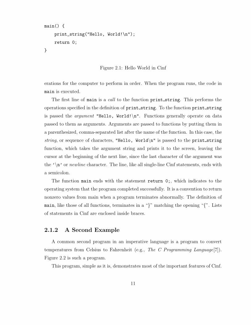
main() {
print_string("Hello, World!\n");
return 0;
}
Figure 2.1: Hello World in Cinf
erations for the computer to perform in order. When the program runs, the code in
main is executed.
The first line of main is a call to the function print string. This performs the
operations specified in the definition of print string. To the function print string
is passed the argument "Hello, World!\n". Functions generally operate on data
passed to them as arguments. Arguments are passed to functions by putting them in
a parenthesized, comma-separated list after the name of the function. In this case, the
string, or sequence of characters, "Hello, World\n" is passed to the print string
function, which takes the argument string and prints it to the screen, leaving the
cursor at the beginning of the next line, since the last character of the argument was
the ’\n’ or newline character. The line, like all single-line Cinf statements, ends with
a semicolon.
The function main ends with the statement return 0;, which indicates to the
operating system that the program completed successfully. It is a convention to return
nonzero values from main when a program terminates abnormally. The definition of
main, like those of all functions, terminates in a “}” matching the opening “{”. Lists
of statements in Cinf are enclosed inside braces.
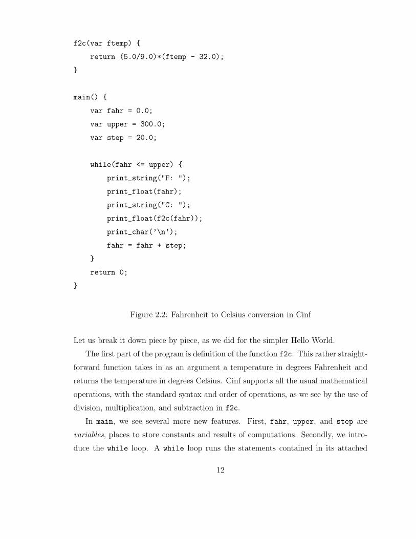
2.1.2 A Second Example
A common second program in an imperative language is a program to convert
temperatures from Celsius to Fahrenheit (e.g., The C Programming Language[7]).
Figure 2.2 is such a program.
This program, simple as it is, demonstrates most of the important features of Cinf.
11
f2c(var ftemp) {
return (5.0/9.0)*(ftemp - 32.0);
}
main() {
var fahr = 0.0;
var upper = 300.0;
var step = 20.0;
while(fahr <= upper) {
print_string("F: ");
print_float(fahr);
print_string("C: ");
print_float(f2c(fahr));
print_char(’\n’);
fahr = fahr + step;
}
return 0;
}
Figure 2.2: Fahrenheit to Celsius conversion in Cinf
Let us break it down piece by piece, as we did for the simpler Hello World.
The first part of the program is definition of the function f2c. This rather straight-
forward function takes in as an argument a temperature in degrees Fahrenheit and
returns the temperature in degrees Celsius. Cinf supports all the usual mathematical
operations, with the standard syntax and order of operations, as we see by the use of
division, multiplication, and subtraction in f2c.
In main, we see several more new features. First, fahr, upper, and step are
variables, places to store constants and results of computations. Secondly, we intro-
duce the while loop. A while loop runs the statements contained in its attached
12

block (the statements between the “{“ and “}”) as long as the attached condition
(the expression inside parentheses) holds true. In this case, the block will be exe-
cuted while the value of the variable fahr is less than or equal to the value of the
variable upper. The contents of the block are mostly familiar: we have calls to the
built-in functions print string and print float, respectively, which print to the
screen strings and floating-point numbers and a call to the user-defined function f2c,
which converts a Fahrenheit temperature to Celsius. The only new statement type
introduced is the last line of the block, which updates the value of fahr to be the
sum of the current value plus the value of step. So, with each time through the loop,
fahr increases by twenty. Finally, main ends with the familiar return 0;, signalling
successful completion.
Readers familiar with programming languages such as C may notice something
missing from this program: type declarations. Had this program in fact been written
in C, it would have been necessary to specify manually that fahr, upper, and step
are all variables holding floating-point numbers. It would also have been necessary to
declare that f2c returns a float, that its argument ftemp is also a float, and that
main returns an integer. The novelty of Cinf is that its type system can infer the types
of variables and the return types of functions from how they are used, rather than
having to explicitly state them. One can still choose to specify types for variables and
functions if one feels it enhances the clarity of a section of code; for example, if one
is writing a library of functions for others to use , it might be wise to declare return
and parameter types, so that others know how to use them.
Note that this does not mean that Cinf is “loosely typed” or “dynamically typed”!
A dynamically typed language is one in which variables themselves do not have types
(only the values stored them in them do) and typechecking is performed at runtime.
The Cinf compiler deduces the types of every variable and function at compile time,
and will fail with an error if, say, an attempt is made to use the same variable as a
float in one place and an int in another. Cinf provides the user with the brevity and
convenience of the syntax of loosely typed languages, while maintaining the safety of
a strongly typed language. Consider, for example, the code in Figure 2.3.
The code in Figure 2.3 will not compile. After reading the first call to add, the
13
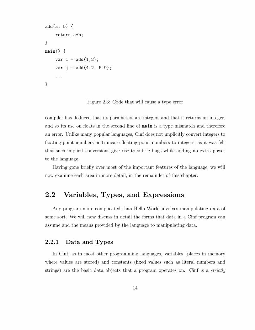
add(a, b) {
return a+b;
}
main() {
var i = add(1,2);
var j = add(4.2, 5.9);
...
}
Figure 2.3: Code that will cause a type error
compiler has deduced that its parameters are integers and that it returns an integer,
and so its use on floats in the second line of main is a type mismatch and therefore
an error. Unlike many popular languages, Cinf does not implicitly convert integers to
floating-point numbers or truncate floating-point numbers to integers, as it was felt
that such implicit conversions give rise to subtle bugs while adding no extra power
to the language.
Having gone briefly over most of the important features of the language, we will
now examine each area in more detail, in the remainder of this chapter.
2.2 Variables, Types, and Expressions
Any program more complicated than Hello World involves manipulating data of
some sort. We will now discuss in detail the forms that data in a Cinf program can
assume and the means provided by the language to manipulating data.
2.2.1 Data and Types
In Cinf, as in most other programming languages, variables (places in memory
where values are stored) and constants (fixed values such as literal numbers and
strings) are the basic data objects that a program operates on. Cinf is a strictly
14
typed language, meaning that every variable has a type, or set of values that it may
hold, and it is a compile-time error to attempt to store a data object of one type in
a variable of another.
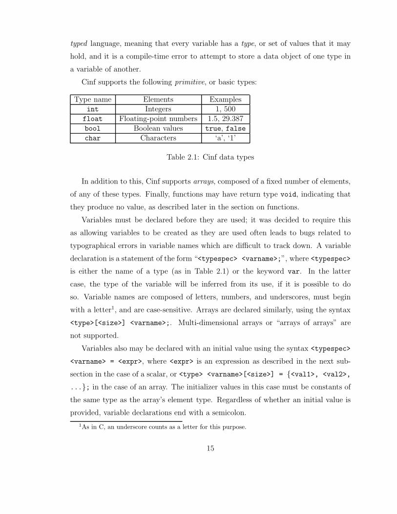
Cinf supports the following primitive, or basic types:
Type name Elements Examplesint Integers 1, 500
float Floating-point numbers 1.5, 29.387bool Boolean values true, falsechar Characters ‘a’, ‘1’
Table 2.1: Cinf data types
In addition to this, Cinf supports arrays, composed of a fixed number of elements,
of any of these types. Finally, functions may have return type void, indicating that
they produce no value, as described later in the section on functions.
Variables must be declared before they are used; it was decided to require this
as allowing variables to be created as they are used often leads to bugs related to
typographical errors in variable names which are difficult to track down. A variable
declaration is a statement of the form “<typespec> <varname>;”, where <typespec>
is either the name of a type (as in Table 2.1) or the keyword var. In the latter
case, the type of the variable will be inferred from its use, if it is possible to do
so. Variable names are composed of letters, numbers, and underscores, must begin
with a letter1, and are case-sensitive. Arrays are declared similarly, using the syntax
<type>[<size>] <varname>;. Multi-dimensional arrays or “arrays of arrays” are
not supported.
Variables also may be declared with an initial value using the syntax <typespec>
<varname> = <expr>, where <expr> is an expression as described in the next sub-
section in the case of a scalar, or <type> <varname>[<size>] = {<val1>, <val2>,
...}; in the case of an array. The initializer values in this case must be constants of
the same type as the array’s element type. Regardless of whether an initial value is
provided, variable declarations end with a semicolon.
1As in C, an underscore counts as a letter for this purpose.
15

2.2.2 Expressions
An expression is something which can be evaluated to produce a value of some
type, which may be stored in a variable (of the appropriate type), used as a condition
in an if or while statement, or used as part of a larger expression. Expressions may
be loosely divided into two categories: constants and compound expressions.
Constants
A constant expression is a literal value of some type. The syntax for constants
for all of the types Cinf support is described in Table 2.1. Note that single-character
literals use single quotes (’), not double(”) Array literals are of the form {<val1>,<val2>, ...}; however, they may only be used to initialize arrays, not anywhere
an array is expected. The only exceptions to this rule are string literals (arrays of
characters), which, using the alternate syntax "string" instead of {’s’, ’t’, ’r’,
’i’, ’n’, ’g’} may be used anywhere an array of characters is expected.
In string and character literals, certain escape sequences, representations of special
characters, are allowed. Table 2.2 is a list of the possible escape sequences in Cinf
character and string literals. Note that each of the two-character escape sequences
corresponds to a single one-character value.
Escape sequence Character\0 NUL character (end of string marker)\n Newline\t Tab\\ Literal backslash\" Literal double-quote character\’ Literal single-quote character
Table 2.2: Escape sequences in Cinf strings
Compound Expressions
A compound expression is composed of either an operator and one or more
operands, where the operator is an arithmetic or logical operator and the operands
16

(if any) are all (arbitrary) expressions, or the name of a function and a list of zero or
more argument expressions. The arithmetic and logical operators are listed in Table
2.3.
Operators with one operandOperator Evaluates to
− Arithmetic negation of operand! Logical negation of operand
Operators with two operandsOperator Evaluates to
+ Sum of operands− Difference of operands∗ Product of operands/ Quotient of operands% Remainder of first operand divided by second
== true if operands are equal, else false
! = true if operands are unequal, else false
> true if first operand is greater than second, else false
< true if first operand is less than second, else false
<= true if first operand is greater than or equal to second, else false
>= true if first operand is less than or equal to second, else false
Table 2.3: Cinf arithmetic and logical operators
An expression in one of these operators takes the form OP exp if OP operates on
one operand, and exp1 OP exp2 if it operates on two. The usual order of operations
applies to these operators: negation is performed first, followed by multiplication and
division; finally, addition and subtraction are done. The comparison operators have
the lowest precedence.
The arithmetic operators may only be applied to integers or floating- point num-
bers, and both operands must be of the same type - mixing types will cause a compile-
time error2. They will produce a value of the same type as their operands. Note that
this implies that integer division is performed on integers, and that the result is not
automatically “promoted” to a floating-point value. MIPS does not support applying
the remainder operator to two floating-point values and so this construction is an
2Values may be converted from one type to another by using the built-in conversion functions;see Table 2.4.
17

error. Furthermore, if one or both of the integer operands to the remainder operator
is negative, the result is undefined by the MIPS specification and as such depends
on the behavior of the machine that SPIM is running on[11]. As such, it is safest to
simply avoid taking the remainder of negative numbers, and care should be taken to
ensure that an expression is positive before taking its remainder.
The comparison operators may be applied to values of any non-array type, as long
as both operands are of the same type - again, this is enforced at compile-time. All
of the comparison operators produce a Boolean value. Finally, the logical negation
operator can only be applied to Boolean expressions. It produces a Boolean value.
A function call expression takes the form name (exp1, exp2, ..., expn), where name
is the name of a function, either built-in or user-defined, and the expi are arbitrary
expressions. When the function call expression is evaluated, the code associated with
the function of that particular name is executed. The built-in functions are listed in
Table 2.4. Note that the first argument to print string, buf must be a character
array capable of holding at least size characters.
Function DescriptionFunctions to read in dataread int() Reads an integer from the console and returns itread float() Reads a character from the console and returns itread char() Reads a character from the console and returns itread string(buf,size) Reads size characters from the console and stores them in buf
Functions to print dataprint int(i) Prints the integer i to the consoleprint float(f) Prints the floating-point number f to the consoleprint char(c) Prints the character c to the consoleprint string(s) Prints the string s to the consoleFunctions to convert data from one format to anotherinttofloat(i) Convert the integer i to a float and return this valuefloattoint(f) Round the float value f to the nearest integer and
return this value
Table 2.4: Built-in functions
The allowed types of parameters for a function (and the type of the returned value,
18

if any), depend on the function3
2.3 Statements and Control Structures
A Cinf program is built out of functions, and a function is composed of a sequence
of statements. Cinf statements are of five categories: assignments, function calls,
blocks, conditional (if) statements, and looping (while and break) statements.
2.3.1 Assignments
An assignment statement takes the form <var> = <val>;, where <var> is a vari-
able that has already been declared in the current scope, and <val> is an expression
that evaluates to a value of the same type as the variable. If the type of the variable
was not provided at declaration time and an initial value was not provided, the vari-
able’s type will be deduced to be the type of the first value assigned to it. Assignment
statements terminate with a semicolon (;).
2.3.2 Function Calls
Function calls, in addition to being expressions, may also be statements in their
own right. The same description and rules provided earlier apply, with the proviso
that the return value is thrown away. Function call statements also terminate with a
semicolon.
2.3.3 Blocks
A block is a sequence of statements enclosed between curly braces({ and }). A
block may be used anywhere a single statement is expected. Blocks exist primarily
to make the code to handle if and while statements cleaner, but there is no rule
against just inserting a block anywhere a statement is expected; it will have no special
effect, beyond executing the statements inside the block in order.
3See the “Functions” section for details of how the compiler figures out these types for user-definedfunctions.
19

2.3.4 Conditional Statements
The if statement is the means provided for conditionally executing code. An
if statement takes either the form if (<expr>) <stmt> or if (<expr>) <stmt>
else <elsestmt>. <expr> must be an expression that evaluates to a Boolean value.
if behaves as would be expected: if <expr> evaluates to true, <stmt> is executed;
otherwise, <elsestmt> is executed (if present), or control continues on to the next
statement. if statements may, of course, be nested; if this is the case, there exists
the possibility for ambiguity. Consider the sequence of statements in Figure 2.4. The
question here is: which if should the else be associated with? Cinf follows the most
common convention and associates a else clause with the lexically closest if; that
is, the if the shortest distance before the else. In Figure 2.4, if expr1 and expr1 are
both true, stmt1 will be executed. If expr1 is true and expr2 is false, stmt2 will be
executed. Finally, if both conditions are false, neither statement will be executed.
if (expr1)
if (expr2)
stmt1
else stmt2
Figure 2.4: Ambiguity in nested if statements
if statements are themselves statements, so conditions can be chained, as in
Figure 2.5.
Finally, in order to have more than one statement in the body of an if or else,
use a block.
2.3.5 Looping Statements
The while statement is the only means, short of recursion, provided for looping
(repetitively executing the same body of code) in Cinf. It takes the form while
(<expr>) <stmt>, where <expr> is an expression that evaluates to a Boolean value.
<stmt> will be executed until expr evaluates to false, or until a break statement is
20

if (expr1)
stmt1
else if (expr2)
stmt2
...
else
stmtn
Figure 2.5: Chained conditions
executed. A break statement is simply the word break followed by a semicolon; when
it is executed, control will immediately pass to the statement immediately following
the while structure. A similar ambiguity to the if/else problem described above
here occurs when while loops are nested: which loop should a break in an inner loop
break out of? The natural answer is that it should break out of the innermost loop,
and that is what Cinf does.
As before, to put multiple statements in the body of a while loop, use a block.
2.4 Functions and Scope
Functions are the building blocks of a Cinf program. Control in a Cinf program
starts with a call to the function main; this function may call other programmer-
defined functions.
2.4.1 Functions
A function declaration consists of a name, a list of parameters, and a block (the
body) of code. In addition, a return type may be specified. A Cinf program consists of
a sequence of function declarations, exactly one of which must be called main. When
a compiled Cinf program is run, main is called and its contents executed.
If types are not specified for any of the parameters, or for the function as a whole
(the return type), then the compiler will attempt to deduce them. Deduction will fail
21

(and terminate the compilation process) if a variable is used in two inconsistent ways
(e.g., first adding an integer to it and then adding a float), or if there exist multiple
return statements from a function with each one returning an expression of a different
type, or if there is simply not enough information. Figure 2.6 is an example of such
an ambiguous program.
f(a) {
return a;
}
main() {
var b;
f(b);
return 0;
}
Figure 2.6: A program with ambiguous types.
If the type of a variable or function is ambiguous, it may be disambiguated by
providing a explicit type declarations. For example, annotating any of f, a, or b
would be enough to make the types ambiguous. One may freely specify the types of
parameters, and functions explicitly; this is an especially good idea if one is writing
code for a library that other people will use.
Function parameters may be of any type (int, float, bool, char or arrays of any
of the above). However, if a function returns an array, it must either be global or one
of its parameters.The results of returning an array from the function where it was
declared are undefined, but likely to be unpleasant4.
2.4.2 Scope
The body of a function is a block, as described in the previous section. Unlike
the blocks associated with if and while statements (or just plain blocks), variables
4For the curious, local variables are allocated on the stack, and so if a local array is returnedfrom a function, the returned value will point to stack garbage.
22

declared inside a function’s body are local to that function; that is, they exist only
when that function is being executed, and can not be accessed from outside the
function. If a local variable has the same name as a variable declared at the program’s
top level (a global variable), it “shadows” the global variable - that is, references to the
variable of that name will yield the local variable, not the global. Variables declared
in a function are usable everywhere in the function from the point of declaration
downwards; even if a variable is declared inside the body of a loop or if statement,
the variable is still introduced into the function’s scope. Cinf does not allow functions
to be defined inside other functions, or functions to be returned from functions, so
this simple two-level scoping rule suffices5.
5The machinery necessary to support a more elaborate scoping scheme exists in the Cinf compiler,but is not exploited in full yet.
23

Chapter 3
Implementation
In the previous section, we described the Cinf programming language from a
user’s perspective. Now, we look at it from the other side of the command line and
examine the details of how exactly a Cinf program is translated to MIPS assembly
code. Before we start, though, we should note that the Cinf compiler is written in
the Ruby programming language. If the reader is unfamiliar with Ruby, an excellent
introduction to and reference for the language is [14].
Like any other compiler, the Cinf compiler is divided into a series of stages, as
illustrated in Figure 3.1. The first stage, the lexer, translates a stream of characters
(the input source file) into a stream of tokens : literals (e.g. numbers, strings, Boolean
values), keywords (e.g. if, while), operators (the various arithmetic and relational
operators), identifiers (variables and function names), and the other units from which
statements, functions, and programs are formed, such as periods, braces, parentheses,
and semicolons. The process is analogous to taking an English sentence as a string of
characters and turning it into a list of words. The parser then takes in this stream of
tokens and outputs a syntax tree - a structured representation of the program shorn
of such details as punctuation. Continuing our English sentence analogy, this may
be considered analogous to turning an ordered list of the words in a sentence into a
sentence diagram1. This syntax tree is then passed off to the semantic analyzer, which
1A sentence is actually more analogous to a parse tree, a data structure that only occurs implicitlyin this compiler, but will be discussed later in the section describing the parser.
24
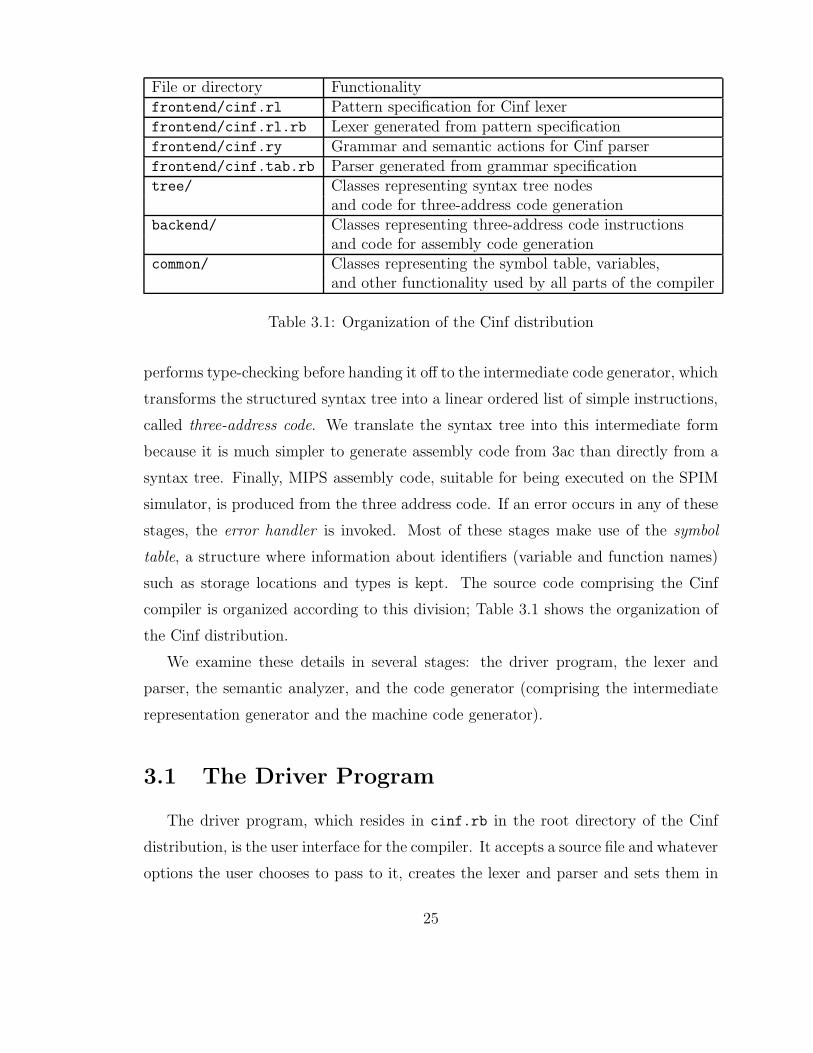
File or directory Functionalityfrontend/cinf.rl Pattern specification for Cinf lexerfrontend/cinf.rl.rb Lexer generated from pattern specificationfrontend/cinf.ry Grammar and semantic actions for Cinf parserfrontend/cinf.tab.rb Parser generated from grammar specificationtree/ Classes representing syntax tree nodes
and code for three-address code generationbackend/ Classes representing three-address code instructions
and code for assembly code generationcommon/ Classes representing the symbol table, variables,
and other functionality used by all parts of the compiler
Table 3.1: Organization of the Cinf distribution
performs type-checking before handing it off to the intermediate code generator, which
transforms the structured syntax tree into a linear ordered list of simple instructions,
called three-address code. We translate the syntax tree into this intermediate form
because it is much simpler to generate assembly code from 3ac than directly from a
syntax tree. Finally, MIPS assembly code, suitable for being executed on the SPIM
simulator, is produced from the three address code. If an error occurs in any of these
stages, the error handler is invoked. Most of these stages make use of the symbol
table, a structure where information about identifiers (variable and function names)
such as storage locations and types is kept. The source code comprising the Cinf
compiler is organized according to this division; Table 3.1 shows the organization of
the Cinf distribution.
We examine these details in several stages: the driver program, the lexer and
parser, the semantic analyzer, and the code generator (comprising the intermediate
representation generator and the machine code generator).
3.1 The Driver Program
The driver program, which resides in cinf.rb in the root directory of the Cinf
distribution, is the user interface for the compiler. It accepts a source file and whatever
options the user chooses to pass to it, creates the lexer and parser and sets them in
25

Lexer
Input source code
Stream of characters
Parser
Stream of tokens
Semantic analyzer
Syntax tree
Intermediate representation
generator
Syntax tree
Machine code generator
Three-address code
Output file
MIPS assembly code
Symbol table
Error handler
Unrecognized token
Syntax error
Semantic error
Allocation error
Figure 3.1: Stages of the Cinf compiler
26
motion, invokes the intermediate representation and code generators, and writes the
output. If the user has specified options for debugging, it will print internal details
of the compilation processs.
The program starts by including the various components that are required for
the compilation process. The first such component is the getoptlong library for
command-line option parsing. It then brings in the lexer and parser, which are
contained in the files frontend/cinf.rl.rb and frontend/cinf.tab.rb. Note that
these files are not actually part of the Cinf distribution; they are generated during the
Cinf install process by running the Rex lexical analyzer generator on frontend/cinf.rl
and the Racc parser generator on frontend/cinf.ry, respectively. Finally, it includes
the code for representing syntax tree nodes by loading the file tree/tree.rb, which
in turn includes all of the files that the syntax tree code is spread over, and the
code that pre-populates the symbol table with the functions in the standard library
(frontend/stdlib.rb). It does not need to explicitly include the file that contains
the code-generation routines, as this is loaded as a prerequisite by frontend/tree.rb.
The driver program then sets default values for the three debugging options that
the compiler accepts; by default, no debugging information is printed, so all three
variables that control printing of debugging information are set to false. Next, the
usage method, which simply prints a help message and exits is defined; this is called
if the compiler is called with not enough or unrecognized arguments. It then creates
an option parser, collects the results of option parsing, and sets debugging flags (or
prints a help message and exits) accordingly. If, after option parsing (which removes
options from the list of arguments), there is not at least one argument to the program,
the program prints the usage message and exits.
If there is an argument (the source file to be compiled), the driver starts the
compilation process. It loads the standard library information into the symbol table
by calling import stdlib (defined in frontend/stdlib.rb), creates a CinfLexer
object, and starts the tokenizing process by passing the supplied argument to the
lexer object’s load file method. If an error occurs during this process, load file
will raise a ScanError exception, which is caught in the main program. The exception
handler extracts the unrecognized string from the exception object’s message field,
27

prints an error message with the string and line number that occurred on, and exits.
If tokenizing succeeded, the driver program creates a CinfParser object, passing
it the lexer object and the parser debugging flag. It then starts the parsing process
by calling the parse method on the parser object; if the debugging flag is set, this
will produce output showing every move the parser makes during the parsing process.
If parsing succeeds, the root of the syntax tree (an object of class ProgramNode)
is obtained by calling the tree method on the parser object, and the second-stage
typechecking process is performed by calling the typecheck method on the tree root.
Finally, if typechecking succeeds, the syntax tree is translated into three-address code
by the method emit 3ac.
Errors that occur during the above process can be one of three types. If the parser
encounters a syntax error, it will raise a ParseError exception; if a type mismatch
or expression with types that cannot be inferred is encountered, a TypeError will be
raised, and finally, if a semantic error such as a reference to an undefined variable or
function is encountered, the syntax-tree construction code will raise a RuntimeError.
The handlers for these exceptions simply print the appropriate error message and exit
the compiler.
If debugging is enabled, the compiler prints the syntax tree in both raw and
more human-readable form by using the inspect and pp methods; both are printed
as the raw form contains more information than the human-readable form. Next,
the contents of the symbol table and the generated three-address code program are
printed to the standard output stream. Finally, if the option to write the intermediate
representation of the program was passed, the compiler opens a file of the same name
as the input file with any extension replaced by .3ac and writes the three-address
code program to it.
The last step in the compilation process is to generate MIPS assembly code from
the intermediate representation, which is performed by the emit mips method. The
compiler then either creates a name for the output file if none was supplied by replac-
ing the input file’s extension with .s, opens the output file, and writes the generated
assembly code to it. If the special file name - was specified as the output file, the
output is written to standard output.
28
3.2 Lexer and Parser
The lexer and the parser together form the front end of the compiler - they take
in source text (an input file) and produce an internal representation of it that is more
easily manipulated. Along the way, they verify that the input at least “looks like” a
valid Cinf program - that is, that it can be produced by the Cinf grammar.
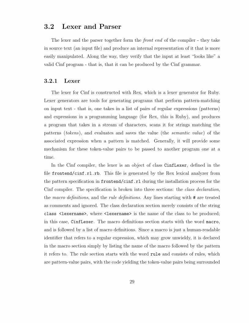
3.2.1 Lexer
The lexer for Cinf is constructed with Rex, which is a lexer generator for Ruby.
Lexer generators are tools for generating programs that perform pattern-matching
on input text - that is, one takes in a list of pairs of regular expressions (patterns)
and expressions in a programming language (for Rex, this is Ruby), and produces
a program that takes in a stream of characters, scans it for strings matching the
patterns (tokens), and evaluates and saves the value (the semantic value) of the
associated expression when a pattern is matched. Generally, it will provide some
mechanism for these token-value pairs to be passed to another program one at a
time.
In the Cinf compiler, the lexer is an object of class CinfLexer, defined in the
file frontend/cinf.rl.rb. This file is generated by the Rex lexical analyzer from
the pattern specification in frontend/cinf.rl during the installation process for the
Cinf compiler. The specification is broken into three sections: the class declaration,
the macro definitions, and the rule definitions. Any lines starting with # are treated
as comments and ignored. The class declaration section merely consists of the string
class <lexername>, where <lexername> is the name of the class to be produced;
in this case, CinfLexer. The macro definitions section starts with the word macro,
and is followed by a list of macro definitions. Since a macro is just a human-readable
identifier that refers to a regular expression, which may grow unwieldy, it is declared
in the macro section simply by listing the name of the macro followed by the pattern
it refers to. The rule section starts with the word rule and consists of rules, which
are pattern-value pairs, with the code yielding the token-value pairs being surrounded
29

by braces after the pattern specification. Inside this code, the value text refers to the
literal string which led to the pattern being matched. The only unusual aspects of the
rules of the Cinf lexer is that rules are provided for all elements of the language, even
punctuation. Unfortunately, due to bugs in Racc, it was necessary to specify these as
token types in the lexer specification rather than just simply letting the parser handle
them in order for the parser to behave correctly. Similarly, only one macro is used,
the BLANK macro matching all whitespace, as the support for macros in Rex did not
work as documented; in particular, it was found that the Rex tool would simply not
expand macros for no apparent reason.
The scan file method on the lexer object loads the file, after which the next token
method may be called to return token-value pairs one at a time. These take the form
of two-element lists [:TOKEN, value], where the first element is a Ruby symbol rep-
resenting the token type and the second is the calculated value of the token. If the
token is an operator, keyword, or punctuation (e.g., {, if,+), the semantic value is
merely the literal text of the token, but as this is subsequently ignored, it hardly
matters - since each of these tokens correspond to exactly one string of characters,
the token type provides enough information. If the token is an identifier (i.e. the
name of a function or variable), the semantic value of the token is also the token’s
literal text, but since there are many character strings that will yield an identifier
token, the semantic value has meaning.
Finally, in the case where the token is an literal scalar value (not an array), the
semantic value will be that value - an integer for a int constant, a floating-point num-
ber for a float constant, the numbers 1 or 0 for a bool constant, and a character
code (in this implementation, an ASCII code) for a char constant. Escape sequences
(single-characters preceded by a backslash representing newlines, the end of string
character (NUL), and other non-printing characters) are converted to the characters
they represent in the process escapes method. String literals have their value (the
actual quoted string) passed on verbatim, whereas non-string array literals are han-
dled in the parser. All whitespace occurring outside of a string literal is ignored, as
is all text occurring after a literal // (comments). The lexer itself is instantiated in
cinf.rb, loaded with the supplied source file, and passed to the instantiated parser,
30

to be used as a state machine that supplies tokens one at a time by means of the
next token method. If at any point, the lexer is unable to match the input stream
against one of its patterns, it will terminate the compilation process with an error
indicating where in the source file the problem occurred. The line number of a given
token is recorded when the token is scanned out of the input file and yielded back up
when next token is called.
3.2.2 Parser
The parser is constructed with the aid of Racc, an LR parser generator for Ruby.
Parser generators take in a description of a context-free language2, called a grammar,
and a set of semantic actions associated with the rules of the grammar, and output
a program that takes in a stream of tokens and attempts to parse it according to
the grammar[1] - that is, it verifies that the string of tokens can be generated by the
grammar3, evaluating the semantic action associated with each rule whenever it can
apply the rule to consume tokens from the input stream. We will discuss the rules
and the semantic actions of the Cinf parser separately, after a brief foreword on how
the generated parser works.
The generated parser parses an input file using the provided lexer object and two
pushdown stacks, the state stack and the value stack. Tokens from the input stream
(the lexer) are pushed onto the state stack (“shifted”) (with their corresponding
semantic values going on the value stack) until the ordered list of tokens on top of
the stack matches some rule of the grammar. At this point, the tokens on the stack
are reduced, or popped off, and replaced with a special symbol representing that rule.
After the semantic action is run, the values of the rule’s components are popped off
the value stack and replaced by the semantic value of the rule application[1]. Symbols
representing rules count as tokens for the purposes of reduction, as a rule may have
other rules as components.
2In this case, the language being parsed must be a LR(1) language; see [1] for an excellentdiscussion for the various classes of context-free languages
3If the reader is unfamiliar with parsing techniques, or context-free languages, [1] is the standardwork on this topic.
31
We will illustrate the parsing process with a brief example. Let the input stream
be the tokens NUM with value 1, PLUS, and NUM with value 3, in that order. The parser
starts by shifting NUM onto the state stack and 1 onto the value stack. It then matches
this against the constant rule and reduces by this rule, popping the NUM symbol off
the stack and pushing on a symbol for the constant rule. The 1 on the value stack is
popped off and replaced with the value that result is set to in the semantic action
for the constant rule; in this case, a new ConstantNode. The state stack now has
one element on it, a constant. The parser notices that it can reduce this again by
applying the expr rule, and does so, popping the constant off the state stack and
replacing it with a symbol representing expr. The contents of the value stack are
left unchanged, as the semantic action for this rule merely passes on the value of the
constant. At this point, the parser can reduce no further, so it shifts the PLUS token
waiting in the input stream onto the state stack and its semantic value, the string
+, onto the value stack. Again, the parser is unable to reduce the state stack, so it
shifts the remaining NUM onto it and pushes the value 3 onto the value stack. It goes
through the same series of reductions as above for this new element; after reduction,
the contents of the state stack are, from top to bottom, expr, PLUS, expr and those
of the value stack are, again from top to bottom, a ConstantNode for the number 3,
the string +, and a ConstantNode for the number 1. The parser matches the contents
of the state stack against the expr rule again and reduces, popping all three of the
elements off the state stack and replacing them with a symbol representing expr. The
application of this rule pops all three values off the value stack and replaces them
with a new AddNode representing this addition expression, completing the parsing of
this string. Figure 3.2 illustrates this process.
Grammar
The Cinf grammar, located in cinf.ry, is heavily inspired by the ANSI C gram-
mar, a formal specification for which can be found online at [6]. It can be broken up,
approximately, into toplevel declarations(function definitions and global variables),
statements (instructions to perform some action with side effects, like assigning an
32

1 + 3
State stack Value stack
Start
+ 3
NUM 1
Shift 1
+ 3
constant ConstantNode(1)
Reduce by constant
+ 3
expr ConstantNode(1)
Reduce by expr
3exprPLUS
ConstantNode(1)+
Shift +
exprPLUSNUM
ConstantNode(1)+3
Shift 2
exprPLUSexpr
ConstantNode(1)+
ConstantNode(3)
Reduce by constantand expr as above
expr AddNode(ConstantNode(1),ConstantNode(3))
Reduce by expr
Input
Figure 3.2: Parsing the string 1 + 3
33
expression to a variable, calling a function with no return value, or repeating a state-
ment while an expression evaluates to true), and expressions (things that produce a
value, such as mathematical operations and logical comparisons). The start symbol
for the grammar is program, which is yielded by toplevel list, as a Cinf program
is composed of a sequence of toplevel declarations.
A toplevel declaration is either a global variable declaration (handled by the
global decl rule), or a function (rule func). In either case, a global declaration
consists of a type, a name, and (optionally, in the case of a global variable declara-
tion), a value (in the case of a function, the function argument list and body, in the
case of a global variable, the token SET and an expression). The type is a decl type
for a function and a defn type for a function, as a variable declaration must have
space reserved for it, whereas a function does not need to have space allocated for its
return value. The defn type and decl type rules both consist of either a basetype
(primitive type name) or a basetype followed by an array specifier, which is a literal
matched pair of brackets (LBR RBR) for a decl type) and a pair of brackets surround-
ing an integer (the array size).This is the source of the one reduce-reduce conflict in
the Cinf grammar, as, given just a basetype, it is ambiguous whether to reduce by
decl type on the spot or reduce by defn type on the spot. Racc resolves the con-
flict by reducing by decl type; since the semantic value is the same for both rules in
this case, this default resolution works4. Function definitions may omit a return type
specifier; in this case, the function’s return type is taken to be auto.
The rule for a function declaration is broken down into three parts: the prototype,
the parameter list, and the block, handled by the rules proto, param list, and block,
respectively. The proto part of a function declaration exists to get the function name
and representative object (more on this later) into the symbol table before the function
itself is fully parsed, so as to allow recursion. The parameter list consists of zero or
more parameter declarations (handled by rule param), surrounded by parentheses
(LP and RP). Parameter declarations consist of a type and a name; they are unique
among the three kinds of variable declarations in that the type is a decl type, not
4There is no way to tell Racc to expect a certain number of reduce-reduce conflicts, so compilingthe grammar will still produce a warning about one reduce-reduce conflict.
34

a defn type. Finally, the block associated with a function is merely a list of one or
more statements surrounded by braces (LB and RB).
Statements (grammar rule stmt) are the blocks that Cinf programs are built
out of; each statement corresponds roughly to an instruction to “do something”.
Statements are either simple or compound, which roughly corresponds to whether
they fit on one line or not; simple statements are terminated with a semicolon (token
SC). Assignments (rule assign stmt), breaks (break stmt), function calls (fcall),
returns (return stmt), and local variable declarations (local decl stmt) are simple,
while conditionals (if), loops (while) and blocks are compound. The rules for break
and return are more or less trivial (a token followed by zero or one expressions,
followed by a semicolon), so we will examine the remaining ones.
An assignment statement is composed of a target, the token SET, and an expres-
sion; a target is either a variable or a reference to an array element. The rule for the
former is trivial; the rule for the latter is a name (ID) and an expression surrounded
by left and right brackets. Unlike in C, assignments are not expressions. The ratio-
nale for this is that allowing assignments as expressions adds no extra functionality
and, more importantly, not allowing expressions as assignments makes it an error to
make the common mistake of writing a = b instead of a == b in the condition of an
if or while statement. A function call statement consists of an identifier followed by
a parentheses-enclosed, comma-delimited list of expressions. Local variable declara-
tions have the same syntax as global declarations. As these are all simple statements,
they terminate with a semicolon.
A conditional statement consists of the token IF, an expression enclosed by paren-
theses, a statement, and optionally the keyword else and another block of statements.
Note that, as written, the rule for conditional statements is prone to the famous “dan-
gling else” problem. - that is, given this code:
if(a == b)
if(b = c)
do_something();
else
35

do_something_else();
it is ambiguous whether the else should be associated with the first or second if.
This manifests as a shift-reduce conflict in the parser, as the parser does not know,
upon encountering the second else, whether to reduce the stack by the if stmt rule
or keep shifting tokens. The default resolution is to keep shifting, which associates
the else with the closest if, which is exactly the desired behavior. A loop is, gram-
matically, more or less the same as a conditional, albeit without the optional else
block and its attendant problems.
The final part of the Cinf grammar is the set of rules for expressions (rule expr).
This is the usual recursive grammar for mathematical and logical operations; an
expression is a constant, a variable, a function call (consisting, as before, of a name
and a list of arbitrary expressions; function calls are legal as both expressions and
statements), an array element, a unary operator (- or !) followed by an expression, a
binary operator between two expressions, or a parenthesized expression. These are all
straightforward, with the possible exception of the rule for negation expressions; since
the same token is used for a subtraction binary expression and we wish for negation
to have a higher priority, we define a “fake” UMINUS operator at the highest priority
level at the top of the file and then later indicate that the unary minus rule has the
precedence of UMINUS by appending the string =UMINUS to the rule text.
The breakdown of the expr rule into constant and cond rules for the various
kinds of constants and conditional expressions is for convenience’s sake only, neither
adding nor detracting from the grammar. The precedences and associativities for
the mathematical and logical operators are listed in order at the top of the file (the
standard C-like order of first the unary operators, then multiplication and division
and modulus, then addition and subtraction, and finally logical operators); as usual,
all the binary operands are left-associative (that is, a op b op c is read as ((a op
b) op c). This approach was chosen over the grammatically unambiguous approach
of breaking the rule for expressions down into rules for expressions, factors, and
terms for simple reasons of clarity and brevity. The grammar has four levels of
precedence, so making it unambiguous without adding precedence information would
36

involve rewriting the expr rule as four different rules.
Semantic Actions
The purpose of the semantic actions associated with the grammar rules are to
build an abstract syntax tree representing the structure of the program, shorn of
the details of punctuation and other incidental syntax. The nodes of the AST are
instances of classes defined in the tree/ subdirectory of the Cinf source tree; there
is one class for each nontrivial rule, with the exceptions of type-related rules, which
will be discussed later. The output of the parser is a tree of these objects, rooted in
the @tree instance variable of the CinfParser object parser.
The semantic actions are standard blocks of Ruby code. In any Racc semantic
action for a given rule, the special variable result corresponds to the semantic value of
the rule application (which will replace the values of the rule components on the value
stack); the variable val is an array containing the semantic values of the components
of the rule (the top n values on the value stack); val[n] is the value of the nth
component. Each nontrivial semantic action (i.e., one that does not just pass on the
semantic value of one of its components) builds the subtree of the abstract syntax
tree corresponding to that rule application by creating a node object (usually based
on the values of the components of the rule) and assigning it to result. Most of the
nontrivial actions, in addition, use the line number that the token that caused the
reduction appeared on; this is accessed through the lineno method on the CinfLexer
object in the instance variable @lexer and is used for error reporting. The fact
that the recorded line number is the token that caused the reduction rather than
the first token of the component is an unfortunate side effect of the way that the
parser functions; it is not a problem in most cases, but can cause confusion when
syntax errors occur on multiline constructs (e.g. leaving off the closing brace of an
if statement with multiple statements in the body.).
The actions are, roughly, of four kinds: trivial actions, list actions, node-creation
actions, and variable-declaration actions. Trivial actions - like the action for block -
do nothing in of themselves; they exist to either drop unnecessary punctuation from
37

the input (e.g. the fact that a block is surrounded by braces is irrelevant to what a
block actually is; a parenthesized expression has the parentheses only for grouping,
they are not actually part of the expression; a defn type or decl type that is not an
array type needs no information beyond the basetype’s value) or to propagate the
value of a rule that was broken off from the main rule for reasons of clarity (e.g. the
separation between expr and cond.) List actions (toplevel decls, param list,
stmt list, arg list, const list) accumulate a list of semantic values through
recursive applications of the rule (and executions of the semantic action); their cor-
responding classes have different behavior in other contexts, but may be treated
identically as far as syntax tree construction goes. Node-creation actions create a
node in the syntax tree corresponding to the rule that caused the reduction; in most
cases, this is an instance of a class defined under tree/ with the appropriate compo-
nent values passed to the constructor, but, as each of the language’s primitive types
is a completely static entity, primitive types are represented by the classes them-
selves, since classes are first-class entities in Ruby. Array types are not static - an
array type is composed of a base type and a size - and, as such, do have objects
instantiated for them; however, because Ruby does not check types of objects but
only requires that they be able to perform all the methods that the programmer calls
on them5, and ArrayType has as instance methods all the methods that the various
type classes have as class methods, this works out well. Finally, variable declara-
tion actions (global decl stmt, local decl stmt), in addition to creating a node
in the syntax tree, also create a Variable object of the appropriate kind and insert
that into the symbol table; this could be done in either the node class constructor
or in the semantic action - in fact, ProtoNode and ConstantNode both insert objects
into the symbol table. Its occurance in semantic actions causes the various kinds of
declarations to have more code in common, which can be factored out into a common
superclass.
With the above in mind, the semantic actions are straightforward to read. A
trivial action just passes on the value of one of the rule’s components, a list rule
5There is irony inherent in using a highly dynamically typed language to build a compiler for astrictly statically typed language.
38

accumulates values in a list, which becomes the action’s value, a node-construction
rule, unless it’s an action for a primitive type, creates a new node, passing it the
values of relevant rule components, and a variable declaration action inserts a variable
into the symbol table and then builds a node. The only action that does anything
fancier than this is the action to create a node in the syntax tree representing a
string literal. The STRING token’s semantic value is a string of characters between
double quotes, with the quotes included. If we just passed this, without modification,
to the ConstantNode constructor, the compiler would end up reserving two more
characters worth of storage in the compiled output than the string actually needs;
on the other hand, Ruby strings are not null-terminated, whereas the strings that
the SPIM simulator (the compiler’s target platform)’s syscalls understand are, so we
have to allocate an extra character for the NUL terminator. The net result is that
when the ArrayType object for the ConstantNode representing the string is created,
we subtract 1 (−2 + 1 = −1) from the string literal’s value’s length, which keeps
everything in order.6
In summary, the parser takes the tokenized input program and produces a tree of
objects representing the program’s structure. The previous two sections have been
wholly concerned with Cinf’s syntax - that is, what valid Cinf programs look like.
In the next section, we examine the details of how the nodes are constructed and
how typechecking is performed, thereby entering into the realm of semantics - what
exactly a Cinf program does when executed.
3.3 Semantic Analyzer
Semantic analysis of Cinf code is done in two separate passes; one from the bottom
up when the syntax tree is built and once from the top down when the second phase
of typechecking is performed. We will examine what happens in each of these passes
on a class-by-class basis
6We do not modify the string itself because it is handy to have it already quoted when the timecomes to allocate space for it in the compiled output, as we can just use the .asciiz directive forallocating storage.
39

3.3.1 Syntax Tree Construction
The syntax tree is built from the bottom up, from the leaves (tokens) to the root
(the entire program); this order is forced on us by the bottom-up nature of the parser.
However, it gives us an excellent opportunity to set up the tree for typechecking and
to perform optimizations like constant folding.
The syntax tree nodes are organized into five files in the tree/ directory of the
Cinf source code, as shown in Table 3.2.
File name Classes containedcommon-nodes.rb Classes inherited from by other nodesexpr-nodes.rb Classes representing expressionsfunction-nodes.rb Classes representing function definitions, calls, and returnsstmt-nodes.rb Classes representing statementstoplevel-nodes.rb Classes representing toplevel declarations and entire programs
Table 3.2: Organization of syntax tree classes
In addition, classes from common/globals.rb, common/symtab.rb and common/types.rb
are used and will be explained as needed. We will examine the classes in these files
in order.
Base classes
Class Node, in tree/common-nodes.rb is the root of the syntax node hierarchy.
It is never instantiated in of itself, but provides functionality that many of the node
classes require. The first of these is the attribute reader th, used by almost every
expression class in the compiler. The th instance variable in nearly every expression
class holds a TypeHolder, defined in common/types.rb, which provides a layer of
indirection for an object’s type. This is done because, as the syntax tree is built, it
is usually often that nodes representing expressions will have the type of one of their
children. Setting the parent’s th variable to one of its children’s ths means that if
the parent or child’s type is ever updated, the change will propagate to the other one,
since they share a typeholder.
40

Node also provides an empty default implementation of the typecheck method so
that typechecking can pass over the entire tree, even over nodes for which it would
otherwise be meaningless, without having to special-case. Finally, Node provides
the unify exprs method, which is the heart of the Cinf type system. unify exprs
and unify prims form a unifier, which compares the types of two expressions and
attempts to make them compatible. The other methods on Node - atom? and
constant? are used in performing constant folding, an optimization that cal-
culates the values of constant expressions such as 3 − 1 or (14 ∗ 2)/7 at compile
time.
The next class in common-nodes.rb is UnaryOpNode, which, as the name sug-
gests, is subclassed by operations that take one operand. Its constructor takes in the
expression the operator acts on, the pretty-printable name of the expression, and a
line number and assigns these to the appropriate instance variables. It also sets the
typeholder of the expression to be the type of the expression it operates on, as noted
above. As this is actually the base class for both the unary expressions and the return
expression, the expr argument may actually be nonexistent, so the assignment of @th
is contingent on expr not being nil, or “empty.”
BinOpNode is one of the most complicated node classes in the compiler. It’s
another base class, so it’s not instantiated directly; nonetheless, there’s a nontrivial
amount of code that two-operand operators have in common and this is where it
all lives. The constructor takes in the left and right operands, plus the printable
name of the operation and the line number and assigns all of these to the appropriate
instance variables. It then tries to unify the types of the left and right operands; if
this fails outright, it catches the exception raised by unify exprs and reraises it with
a little more information. Finally, if the left and right operands are both constant
expressions, it performs the appropriate operation on them (via the do op method
implemented in subclasses) and stores it in the instance variable @val and sets the
@constant flag; this is most of the work involved in the constant folding, described
above. It explicitly does not set the type of the expression itself, as this will vary on
the particular binary operation.
ScalarOpNode is a subclass of BinOpNode that ensures that both its arguments
41

are scalar values (not arrays). All of the binary operations except assignment subclass
this. Its constructor simply checks that both arguments are scalars (and raises an
error if they’re not) before passing control to the BinOpNode constructor.
DeclNode is the superclass of the node classes representing local and global vari-
able declarations. The constructor takes in the name of the variable being declared, a
default value (which may be nil, as variables may be declared without an initializer
expression), a type name (which may, of course, be AutoType), and a line number.
It stores the line number in an instance variable and looks up the variable name in
the symbol table (where it’s guaranteed to be, as it was inserted in the appropriate
semantic action). If a initializing value (defval) was given, it tries to unify the types
of the variable and the value; if not, it creates a new TypeHolder to hold the supplied
type. Either way, it stores the initializer in @defval.
Expression classes
ConstantNode, the first class in tree/expr-nodes.rb is one of the simplest non-
trivial class in the file; as such, it is a good place to start explaining the structure
of Cinf expressions. It’s especially simple because a constant by definition always
has its type known. As such, the ConstantNode constructor starts out by storing
the constant value in the instance variable @var and creating a new TypeHolder for
the provided type and storing it in the usual place (instance variable @th). The rest
of the constructor deals with how the constant is actually stored. If the value is an
integer and is between MIN IMM and MAX IMM; that is, if it fits in a 16-bit signed value
(the size of the immediate field in a MIPS-32 instruction), then it can be stored as
an immediate value without having to allocate memory for it in the compiled output.
If not, the constructor generates a name for the constant based on its type and value
and looks it up in the symbol table. If there’s already an entry for it, then it reuses
that; otherwise, it creates a new global variable with that name, the appropriate type,
and the constant value as initializer and stores it in the symbol table.
The next class in expr-nodes.rb, ConstListNode is a special-cased class for non-
string array literals, as it was impossible to scan array literals as array literals in the
42

lexer. A new array literal is empty; the first element in it sets the type of the array,
and any elements that do not match that type cause type errors (raised from the
push method); there is no inference logic needed because array literals are required
to consist only of constants.
A VariableNode, as the name suggests, represents a reference to a variable in
a program, either as something being assigned to in an assignment statement or as
something yielding a value in an expression. The constructor for a VariableNode
doesn’t do much; it looks up the given variable name in the symbol table, raises an
error if it’s not there, and sets the node’s typeholder to the that of the variable.
An object of class ArrayAccessNode can appear anywhere a VariableNode can,
and so there are some major similarities between their implementations. That being
said, the differences are great enough that it was not worth making them descendants
of a common superclass. The constructor starts off by saving the line number the
array element was referenced on and looking up the array variable in the symbol table,
raising an error if it isn’t there. It then starts from the knowledge that the indexing
expression must be an integer and propagates that information onto the index’s type
holder if it is still of an unknown type; if, after this, it’s still not an integral expression,
a type error is raised. The index expression subtree is stored in the @index instance
variable.
The ArrayAccessNode constructor then moves on to consider the type of the
array itself. If it is of unknown type (that is, if @arr.th.type is AutoType, we can
now change that to a new ArrayType of AutoTypes, as we are indexing it. This
code handles the case where an array is passed to a function, but doesn’t have type
information declared for it in the parameter declaration. If after this process, the
array’s type is still scalar, then an error is raised, as it is meaningless to index a
scalar value.
As the ArrayType object in the array’s @th variable itself has a type method and a
type= method, and the only requirement on the contents of a node’s @th variable are
that it support type and type= methods, we use the array type itself as a type-holder
for ArrayElements. This has the major advantage that if we are able to infer the
type of any element of an array, we automatically infer the element type of the entire
43

array, and since typeholders themselves are never overwritten, this works perfectly.
Finally, an ArrayElement is created based on the array and index to provide the
low-level implementation of an array access.
UnaryMinusNode objects represent negation expressions. The class is a subclass of
UnaryOpNode, so the constructor starts off by calling the constructor for UnaryOpNode.
It then ensures that the passed-in expression is either numeric or of unknown type
and raises an error if this is not the case. Note, however, that it cannot infer the
type of the expression here as, while it must be numeric, it cannot immediately be
determined whether the type should be integral or floating-point. It does the usual
typeholder setup and then, if the expression is constant, calculates the negation of
its value, stores it, and sets the constant flag; again, this is the constant folding
optimization.
LogicalNegateNode, like UnaryMinusNode is a subclass of UnaryOpNode, and the
constructor starts off by calling its constructor. The major difference after this is
that since we know that the operand must be Boolean, we can infer its type then and
there, which the code does. If the operand is still not Boolean after type inference,
it raises a type error. Finally, after storing the typeholder, it calculates the logical
negation of its value and stores it, setting the constant flag as usual. True and false are
represented in Cinf internally by the numbers 1 and 0, so bitwise XORing a Boolean
value with 1 will flip the low bit, which is exactly what we want here.
Class NumericBinOpNode is a further refinement of ScalarBinOpNode that merely
ensures that both its arguments are numeric, on top of the guarantees already pro-
vided by ScalarBinOpNode and BinOpNode. It raises an error if this is not the case,
but otherwise does nothing different from its parents.
ArithmeticBinOpNode is the parent class of all the mathematical operations. In
addition to calling the constructor of NumericBinOpNode, it sets the expression’s type-
holder to the typeholder of the left operand (chosen arbitrarily, since both most have
the same type by the end of the typechecking process.). All of the binary mathemat-
ical operators (DivNode, MulNode, ModNode, AddNode, SubNode are trivial sub-
classes of ArithmeticBinOpNode; they call the constructor passing in a name for
the operator (’+’, ’*’, etc) and implement a do op method that performs the specific
44

operation and is used in constant folding.
EqNode and NeqNode are subclasses of ScalarBinOpNode rather than ArithmeticBinOpNode
as any two scalar values can be compared for equality. They fix their expression types
as BoolType, but are otherwise identical to the above arithmetic operations.
LogicalBinOpNode is a subclass of ArithmeticBinOpNode that just sets the ex-
pression’s typeholder to a new one wrapping BoolType after running the super-
class constructor. All of the non-equality relational operators (LtNode, GtNode,
LeqNode, GreqNode) subclass it; they are, in every way, like the arithmetic node
classes.
Statement classes
AssignmentNode, the first class in tree/stmt-nodes.rb represents one of the
most important statement types in an imperative language; as such, we will begin
our overview of how syntax subtrees for statements are built here. AssignmentNode is
a subclass of BinOpInstr, and its constructor is not very different; it merely ensures
that only scalar values and strings are being assigned to variables and raises an error
if this is not the case before calling the superclass constructor. Normally, this would
only allow the assignment of scalar values, but C has a peculiarity of syntax and
semantics that allows string literals to be assigned to variables, and it was decided
to faithfully emulate this quirk in the name of making the language more familiar to
programmers used to C. Furthermore, passing a constant string to a function is such
a very common case that it could be considered a good idea to support it, regardless
of whether C did it or not. Finally, it sets the statement’s type to void, as statements
do not return a value.
Class IfNode represents a conditional statement. Its constructor is very simple;
it just takes in the line number and objects representing the condition, body, and
else statements (if any) and stores them in instance variables. Like many of the
classes in this file, the real functionality for this class happens in the intermediate
code generation stage. The constructor for WhileNode is similar, except that a while
loop only has one block of statements associated with it.
45

The NullaryOpNode class is a vestigial hold-over from a previous version of the
language that became Cinf; the only class implementing it is BreakNode. However,
the constructors for both classes are short, so we will cover them here. The BreakNode
constructor stores the line number and passes control to the NullaryOpNode construc-
tor, which stores the node’s printable name. Again, most of this class’s functionality
is in the intermediate code generation stage.
LocalDeclNode objects represent declarations of local variables. The local variable
of the given name and type has already been created by the time the constructor
is entered, so the constructor simply calls DeclNode’s constructor, passing it the
appropriate arguments. The only thing left to do is to save the variable on the list
of the current function’s local variables; this information is used later in allocating
stack space for a function invocation.
The final class defined in tree/stmt-nodes.rb is StmtNodeList, which is another
accumulator class like ConstNodeList and works in almost exactly the same fashion;
the differences are not worth mentioning at this point.
Function Classes
The source file tree/function-nodes.rb contains the most complicated classes
in the compiler - those dealing with function definitions, calls, and returns. The
first class in the file, FuncCallArgListNode is another “list node” class, as seen
earlier. The major difference is that here it is useful for the class to behave more
like an Array; that is, it is useful for it to be indexable and iterable. In order to not
have to duplicate a great deal of code with methods wrapping the array @args, we
instead implement the special method method missing. If a a method is called on a
FuncCallArgListNode object and it does not match the name of any of the methods
explicitly defined in the class, Ruby will call the method method missing, passing
it the name of the method called and any arguments collected in an array. The
implementation of method missing simply passes on the method call to the array
@args that the class wraps; in short, the object behaves as a proxy for the internal
array, in addition to its other functionality. This means that in addition to having
46

all the functionality of a Node, the class also effectively has all the functionality of an
Array - a useful thing to be able to do, considering that Ruby doesn’t allow multiple
inheritance.
An instance of FunctionCallNode represents a function call. Its constructor takes
in the name of the function being called, the list of arguments to the function (the
class for which was defined above) and a line number. Like most of the node class
constructors, it begins by storing these in instance variables. It then looks up the
Function object for the function being called in the symbol table, raising an error if it
has not been defined. The number of calls made to the function so far is incremented
(this information is useful in typechecking later), the argument list is checked to make
sure that the right number of parameters are passed to being passed to the function,
and finally, the typeholder (and type) of the node is set to the function’s return type.
Class ReturnNode represents a return statement in a function. The logic in its
constructor (and later, typechecker) are slightly contorted by the fact that the type
of the expression being returned, if any, is inexorably bound up with the return type
of the function, which is dealt with elsewhere in the tree. The constructor starts
off by saving the line number, like most other interesting node classes. If there is no
return expression provided, the instance variable @eth, which contains the typeholder
of the type of the value being returned from the function, is set to a new TypeHolder
holding VoidType; if not, it is initialized to the typeholder of the expression being
returned. Next, it grabs the current function (which will be the function the return
is associated with), stores it in an instance variable, and tries to unify the type of
the expression being returned with the known return type of the function. As usual,
if unification fails, a type error is raised; if unification is inconclusive (if both types
are still unknown), this is dealt with later. Finally, the superclass (UnaryOpNode)’s
constructor is called, the typeholder for the return itself is set to that of the function,
and the return is stored in the function’s list of returns; this list is used later for
typechecking.
ParamListNode is yet another list-node class; the major difference here is that
a function is allowed to take zero parameters, so the constructor checks for a nil
argument before storing it in an instance variable (or storing a fresh array, if it is
47

nil). This class uses the same “proxy” technique as ArgListNode to provide Array-
like behavior.
The ParamNode class, like the various DeclNode classes, represents a variable
declaration (in this case, the the declaration of a formal parameter for a function).
As is the case with the other declaration nodes, the relevant variable has already
been inserted into the syntax table by a semantic action by the time a ParamNode is
created, and so all the constructor does is ensure that the given type in the declaration
is a reasonable (i.e. non-void) type, looks up the variable in the symbol table and
saves it in an instance variable, and set the object’s typeholder appropriately.
A ProtoNode represents a function’s prototype, containing its name, return type,
and formal parameter list. The constructor for ProtoNode stores the line number,
name of the function, and parameter list in instance variables. It then creates a new
Function object representing the function being defined with this information and
inserts it into the symbol table under this name; this is done in order to get name
and type information into the symbol table before the function definition is finished,
so as to enable recursion and inference of type information about the function from
recursive calls. Finally, it sets the current function to this function; this is used by
return statements to find the function to attach themselves to.
The final, and most complicated class in function-nodes.rb is FunctionNode,
which actually builds a node representing a function definition from prototype in-
formation and the lists of local variables, and returns. The constructor starts off
by extracting the parameter list, name, function object, and list of returns from the
prototype and the passed-in block of code from its arguments and storing them in
instance variables. It then checks to see if the list of returns is empty; if this is the
case and the function was declared as returning a non-void type, a type error is raised;
otherwise, the function’s return type is inferred to be void and has a return type set up
properly. Conversely, if the function is declared as void, the constructor ensures that
if there are any returns, none of them return an actual value. The FunctionNode’s
return type(holder) is then set to that of the Function.
Next, the current function variable on the Function class is cleared, as the function
declaration is over at this point. For the same reasons, the locals and parameters are
48

removed from the symbol table; all references to them have been resolved and we
wish to clear the way for other functions to reuse those names. Finally, in a block of
code that perhaps should have been left to a later stage of the compilation process,
memory or register addresses are allocated for parameters. Locals cannot be allocated
at this time because the number of temporary variables that will be necessary is not
known.
Toplevel Classes
The classes in tree/toplevel-nodes.rb are even simpler than those in the State-
ment Classes section, so we shall spend even less time on them. TopLevelListNode
is another list class, with nothing to distinguish it from any of the other list classes
insofar as how it is built. GlobalDeclNode needs no special constructor code over
what is already in DeclNode - the variable was already inserted into the symbol table
by the semantic action for the rule - so it has none. Finally, a ProgramNode is more
or less a wrapper around a list of toplevel declarations.
3.3.2 Typechecking
The compiler makes two passes on the syntax tree in which type-checking and
propagation of type information are performed. The first, bottom-up, pass, in which
the syntax tree and its associated type relations are built was discussed in the previous
section; in this section we once again go over the syntax tree classes and go over how
the second, top-down typechecking pass is performed. Before doing so, though, we
examine the manner in which types in Cinf are actually implemented
Cinf Types
Types in Cinf are represented by the classes in common/types.rb. The primitive
types - int, char, float, and bool - are represented by the classes of the appropriate
names. That is, they are actually represented by the classes themselves; since classes
are first-class objects in Ruby, they can be passed around, have methods called on
them, and so on like any other object. The rationale for this is that the information
49
about any given primitive type is completely static - all integers have identical type
information, as do all floats, and so on.
All the primitive type classes, including AutoType which represents a currently
unknown type inherit from class Type, which defines default implementations of the
standard type methods. The methods are generally self-explanatory; they express
properties of the type like being numeric or being a scalar. The defval method
returns the default value for variables of the type in question; global variables of that
type will be initialized to this value if no initializer is given. For all of the types except
FloatType, this is merely 0, as Booleans, integers, and characters are all implemented
as integers. The mkconst method takes in a value and generates a name for the global
variable for a constant of the appropriate type; for all of the scalar types, this is based
on the value of the constant. This has the advantage of reusing constants instead of
generating duplicates. The same type? method, as the name suggests, tests to see
if two types are the same. The size method returns the number of bytes a variable
of the given type takes up in memory; this is 4, or the size of a MIPS word for all
of the scalar types. However, for compatibility with SPIM system calls, characters
must be “packed” into arrays when they appear in them; that is, arrays of characters
must be arrays of bytes rather than arrays of words. The psize method returns the
packed size of the type; CharType is the only type class that overrides this. Finally,
the constdir method returns the assembler directive that is used for reserving space
in the compiled output.
Unlike primitive types, array types have non-static information associated with
them: the element type and the size. As such, array types are instances of class
ArrayType instead of just being static classes; because Ruby is dynamically typed
and only cares about what methods an object implements, and ArrayType methods
implement all the important methods that Type classes do, this works out well. The
constructor for an ArrayType takes in a type and size (both of which may be unknown,
as they may not have been inferred yet), stores them in the appropriate place, and,
if it doesn’t already exist, creates an entry in the @@constctrs hash. This variable
is used in generating names for constants, as the name would suggest; since arrays
may be of arbitrary length (and since character arrays can contain spaces), there isn’t
50

really any good way of generating a name for an array based on its value.
The calc size method, as the name suggests, calculates the size an array of the
given type and size will take up in memory; it multiplies the type’s packed size by
the number of elements; as this is a size in bytes, it rounds the entire thing up to
the nearest multiple of four (one word) for neatness. The constdir method works
as described above, generating a constant name based on the array element type
and the value of the appropriate slot of @@constctr. reserve global provides the
assembler directive to reserve enough space for the array in the compiled output,
while same type? checks that the type being compared against is both an array and
of the same element type (size is not part of an object’s formal type). The final class
in types.rb is the simple TypeHolder, which we have already introduced.
Now, having explained how types are actually implemented in Cinf, we will go on
to examine how the second typechecking pass through the syntax tree works.
Typechecking in the Common Classes
The default implementation of typecheck in Node does nothing; it is merely there
to make it possible to iterate over nodes and call the method without the need for
special cases for each node type. The typecheck method for UnaryOpNode simply
dispatches typechecking to the expression, since the unary operations are so varied in
type behavior as to make further generalization impossible.
In BinaryOpNode, the default typecheck method typechecks each of the operands
before trying to unify their types as before. The second call of unify exprs is useful
because new type information will have been added since the first pass through -
that is the entire point of the typechecking process. ScalarOpBinNode#typecheck
calls its parent class’s implementation of typecheck, then checks to ensure that both
operands are scalar, raising an error if they’re not. Finally, in DeclNode, we typecheck
the default value (if any), then try to unify the variable type with the default value
type, raising a (more informative than default) error if the types don’t match.
51
Typechecking at the Toplevel and in Statements
The typechecking process is a top-down traversal of the syntax tree, so we will
begin at the root, by looking at ProgramNode. The typecheck method here is triv-
ially simple; it passes the request on to the StatementListNode in @decls. In
StatementListNode, the action performed is almost as trivial; it loops over the list
of toplevel declarations and asks each to typecheck itself. GlobalDeclNode needs no
special typechecking behavior; it is handled in DeclNode as discussed above.
Typechecking assignments is trivial; BinOpNode and ScalarOpNode do all the
heavy lifting. Likewise, as before, typechecking for LocalDeclNode is handled in
DeclNode.
Typechecking if statements is almost as simple; the class’s typecheck method
calls typecheck on the condition expression, the body of the if, and the else block
if there is one. If after all of this, the conditional is still not Boolean-typed, it will
raise a type error. As before, the typechecking pass for a while statement is the same
as that for an if, without the extra step for an else block. The statement blocks
in both of these are StmtListNodes, the typecheck for each of which simply iterates
over the statements in the list, calling typecheck as it goes.
Typechecking Expressions
The first two expression classes, ConstantNode and ConstListNode, both deal
with constants, the types of which are always known; as such, they use the default
do-nothing typecheck method. A VariableNode, likewise, can only have its type
inferred in more complex expressions, so it too uses the default implementation.
Likewise for ArrayAccessNode; the only typechecking that could have been performed
here at this stage would be to ensure that the index was an integral expression, and
we already did this when the node was constructed.
UnaryMinusNode, in its typecheck method, simply typechecks the expression
and ensures that the value is numeric, raising an error if it is not. In contrast,
as might be expected, LogicalNegateNode passes off responsibility for typechecking
to UnaryOpNode. This comes down to just typechecking the expression that is being
52

negated, as the type of the overall expression is forced to be Boolean since it is a
logical operation, which is not the case with UnaryMinusNode.
NumericBinOpNode calls its superclass’s typecheck method and then, if that suc-
ceeded, ensures that both operands are numeric. ArithmeticBinOpNode (and its
subclasses, all the arithmetic expression nodes), can just rely on this implementation,
as the typeholder for the expression was set appropriately in the constructor. The
same is true for the various relational operator nodes and their superclasses.
Typechecking Functions
The final set of typechecking code to examine is, as before, that dealing with
function calls and returns. We begin with FuncCallArgListNode which, fortunately,
requires no special typechecking logic of its own, as checking arguments against formal
parameters is performed in FunctionCallNode, which we will proceed to examine.
Before we examine the typecheck method itself, though, we need to examine the
specialized unifier that it uses. There are two main differences; firstly, the unifier
(unify exps and unify pt) takes an extra parameter that is the index of the param-
eter/argument pair in their respective lists and secondly, if all calls to the function
have been checked and there are still indeterminate types, an error is raised. The ra-
tionale for this is clear; if, by the last call, we have not gathered enough information
to infer the type of a parameter, we will never have enough, and so raising an error is
the only sensible response. The index parameter is just used to provide a more useful
error message.
Now we can look at the typecheck method itself. First, we iterate over the list
of arguments to the function and typecheck each expression. After this, we iterate
from 0 to the largest index of the parameters list (size − 1), and try to unify each
(parameter,argument) pair. If this succeeds, we increment the number of checked
calls to the function by one.
The typecheck method of class ReturnNode, if there is an expression being re-
turned, first typechecks the expression. Then, it tries to unify the type of the expres-
sion with the type of the return statement (which is by now the same as the return
53

type of the function it is returning from). If this succeeds, typechecking completes
successfully; otherwise, an error is raised.
ParamListNode, ParamNode, and ProtoNode are not typechecked in and of them-
selves, but are used in FunctionCallNode and FunctionNode. Having already gone
though the former, we now proceed to examine the latter, which is trivial, as all it
does is typecheck the block of statements. Typechecking of returns and parameters
has already been done in other classes.
3.4 Intermediate Representation Generation
After syntax tree construction and second-phase typechecking has been performed,
the net result is an abstract syntax tree with all relevant semantic information filled in.
In theory, it would be possible to translate this tree directly into assembly language
for the target machine; in practice, the conversion process can be made much easier
if we first convert the syntax tree into another intermediate representation. The
intermediate representation used in the Cinf compiler is called three-address code,
or 3ac. A 3ac program is a sequence of statements of the form tgt := src1 op
src2, where tgt, src1 and src2 are variables and op is a mathematical or logical
operation[1]. The effect of the statement is to assign the result of performing op on
src1 and src2. Of course, not all 3ac instructions fit this pattern; some, like negation
or logical negation only take one source operand, and some like the instructions
necessary for control flow do not perform any assignments at all, but the majority of
the 3ac instructions follow this rough pattern.
Three-address code is generated from the syntax tree - in which, recall, operands to
expressions may be expressions in their own right - through a process called lineariza-
tion. The linearization process is, essentially, a post-order traversal of the syntax tree
- to generate the 3ac for a node, we first generate the 3ac for its operands (saving the
temporary variables that they will put their results in), and then generate the code
for the node itself, using those operands. Of course, non-expression statements like
if and while require slightly more work, but this is the general idea.
The 3ac instructions are defined in backend/3ac.rb, but as all of them have
54
essentially trivial constructors, we will discuss any necessary details as they come up
in the linearization process. Table 3.3 is a list of all three-address code instructions.
Operators with trailing periods in Table 3.3 operate on floating-point values; all others
act on integral (including character and Boolean) values.
3.4.1 Linearizing Common Node Classes
Node obviously contains no code to perform linearization; the different node classes
are just too different for there to be enough commonality to factor out. We therefore
move on to UnaryOpNode, for which there is code that has been factored out.
The method on UnaryOpNode that performs linearization, as is the case for all
nodes that emit 3ac, is called emit 3ac. It takes in an optional parameter called
out, which, if given, holds the place to put the value of the entire expression. This is
for an optimization called unnecessary temporary elimination. Consider the following
Cinf statement : a = -b, where a and b are variables. A “naive” 3ac generator might
produce the code in Figure 3.3, where T1 is a generated temporary. Clearly, this can
T1 := -b
a := T1
Figure 3.3: “Naive” 3ac for a = -b
be reduced to just the instruction a := -b. This is accomplished by, whenever an
assignment is encountered, passing the variable being assigned to as the out param-
eter to the expression on the left, if this is possible. For more information, see the
description of how assignment is linearized.
Returning to the description of linearization of UnaryOpNode, the method first
generates 3ac for the expression being operated on, if one exists; recall that return
statements are UnaryOpNodes, but do not necessarily have an operand. The expres-
sion’s emit 3ac returns a variable in which its output is stored; this will usually be
a generated temporary variable. Finally, this temporary (called operand) and the
out variable are passed to emit spec, which is implemented by all the subclasses of
55

UnaryOpNode. emit spec handles the node-specific details of linearizing that partic-
ular kind of expression and returns the variable in which the result of that expression
will be stored, so the entire emit 3ac method returns the correct variable.
BinOpNode is able to factor more functionality out into its emit 3ac method than
UnaryOpNode. Like all the other emit 3ac methods, it takes in the same optional out
parameter for the same optimization. It begins by testing to see if the operation’s
type is void; if so, then it must be an assignment and rather a lot of code can be
skipped over. We will examine the non-assignment (binary-operation expression) case
first.
Earlier when we looked at how nodes representing expressions are built, we saw
that constant expressions have their values calculated when the syntax tree is built.
Here, we actually use that value that was precalculated before. As in ConstantNode’s
constructor, if the constant value is an integer requiring no more than 16 binary
digits (including a sign bit) to represent, then we can (eventually) represent it in the
generated assembly code as an immediate value in a load instruction and create and
return a IntegerConstant accordingly. If the value is too large to fit in an immediate
field or is a float, we instead must allocate a global variable for it, if one has not already
been allocated; the code here is more or less the same as the corresponding code in
ConstantNode. Regardless of whether we had to create the variable or looked up
an existing one, we return this variable as the place where the value of the constant
expression will live.
If the expression is not a constant, then more work is necessary. First, if no
out parameter was supplied, we generate a new temporary local variable (using
SymbolGenerator.gensym to supply a new guaranteed-unique name) and allocate
space for it. Then, we generate 3ac for the left and right operands of the instruction.
Finally, if one of the operands is a floating-point type (remember, both operands are
guaranteed to have the same type by now), we call the emit specf method, passing it
the place to store its result (out) and the places where the values of the left and right
operands may be found (lvar and rvar). Otherwise, the operands are integral and
we call the emit spec method. Because the MIPS processor that Cinf targets, like
most CPUs, treats integers and floating point numbers very differently, it is cleaner
56

to separate integer and floating point instructions at this stage rather than during
assembly code generation. Finally, the method returns the out variable.
ScalarBinOpNode adds no functionality to the BinOpNode linearizer (it exists
solely for the typechecking functions it provides), so we proceed to DeclNode. DeclNode’s
emit 3ac method is very simple: if there is a default value, it generates code for the
default value, passing it the variable being declared as the place to put its value,
and returns the result of emitting this code. Both of the subclasses of DeclNode
(LocalDeclNode and GlobalDeclNode) override this with methods that have more
complex behavior.
3.4.2 Linearizing Statements and Toplevel Declarations
Since most of the toplevel classes exist purely for structuring the parse tree, we
will go over them briefly and then proceed to statements. Class TopLevelListNode’s
emit 3ac method, as one might expect, just iterates over its list of declarations,
emitting 3ac for each one. Class ProgramNode actually creates an object to hold
the generated 3ac instructions before generating code for its toplevel declarations.
To linearize a GlobalDeclNode, after first calling the superclass constructor, is also
simple. Here is where the other half of the unnecessary temporary removal elimination
is performed: if a compound expression was being assigned to the variable, then no
further code needs to be emitted, since when we generated the 3ac for the expression,
we passed it the variable as the place to store its value. However, if the default value
was a variable, constant, or array access (referred to as atoms, because their 3ac
value is something that acts as a variable rather than one or more statements of 3ac
being appended to the growing program), then we have to generate an assignment
instruction to store the value in the variable (if there is a default value).
To linearize an AssignmentNode, first we get the underlying variable (or array
element) by calling emit 3ac. We then get the output value of the right side by
linearizing it, passing it the variable on the left as the place to store its output. We
then go through the same process we did with DeclNode, generating an assignment
instruction only if it was necessary.
57

Linearizing a if is the first really nontrivial case we have encountered. We be-
gin by generating the 3ac for the condition (and storing the output variable) and
a name for a label that will go after the if block. If there exists a block of else
statements, we also generate a label that will go before that block. We then generate
a BranchFalseInstr, which will, if its first argument is false (equal to 0), branch to
the label that is its second argument. We then emit the 3ac for the statements in the
body of the if, followed by a JumpInstr targeting the label after the if block, as we
wish to skip over the else block. Finally, we emit a LabelInstr instruction for the
label for the else statements and the 3ac for the else block itself.
If there are no else statements, the code generation is similar. We emit a
BranchFalseInstr examining the value of the conditional and targeting the label
after the if statement, and emit the 3ac for the body of the if. Either way, we end
by emitting the label for after the end of the if.
The linearization process for WhileNode bears some resemblance to that to IfNode,
but has some major differences. Firstly, since while loops may be nested, we need a
way for a given break statement to find the place it should jump to; this is imple-
mented through class BreakStack, which is just a stack. emit 3ac starts by gener-
ating labels for before and after the loop; it then emits the label for the beginning
of the loop and pushes the label for the end of the loop onto the BreakStack. We
emit the code for the loop conditional, emit an instruction to jump out of the loop
if it is false, emit the 3ac for the body of the block, emit a jump going back to the
beginning of the loop, emit a label for after the loop, and finally pop the end-of-loop
label off the BreakStack.
We will, as usual, skip over the vestigial NullaryOpNode and proceed directly to
BreakNode. To emit 3ac for a break, the method first checks to see that the statement
actually occurs inside a while loop; if not, an error is raised. Finally, it simply emits
a jump to the label at the top of the BreakStack.
The emit 3ac method of LocalDeclNode starts off by allocating space for the
variable. It then emits a LocalInstr signifying that a local variable was declared
at this point. Finally, does the same trick for elimination of unnecessary temporary
variables we saw in GlobalDeclNode and emits an AssignInstr assigning an atom’s
58

value to the variable being declared if necessary.
Finally, as one might expect, to emit 3ac for a StmtListNode, we just iterate over
the list of statements and emit 3ac for each one.
3.4.3 Linearizing Expressions
The simplest expression, a ConstantNode also has simple 3ac: emit 3ac returns
the underlying variable (or variable-like object; if it’s small enough and of the right
type, it will be an IntegerConstant, as mentioned earlier. VariableNodes trans-
late to 3ac in the same manner. ArrayAccessNodes have to emit 3ac for the index
expression (the output variable for which gets stored in the index variable of the
underlying ArrayElement, but the emit 3ac method returns said ArrayElement.
ConstListNodes exist solely as conveniences to the syntax tree, so there is no need
to generate 3ac for them.
As mentioned earlier, the classes that inherit from UnaryOpNode implement emit spec,
which is called from the parent’s emit 3ac. In UnaryMinusNode, the method starts
with the same constant folding code that we’ve seen in several classes now; if it was
determined that the expression is a constant, we either create an IntegerConstant
with that value and return it or, if it won’t fit in one, create a global variable to
hold the precalculated constant value and return it. If it’s not constant, we create
an output variable and allocate space for it if one wasn’t passed in and emit either a
NegateInstr or a NegateFInstr operating on the operand and putting its value in
the output variable, depending on whether the operand is an integer or a float. The
method returns out, the output variable,since a UnaryMinusNode is an expression
and therefore produces a value.
Since a LogicalNegateNode operates exclusively on Boolean values, the code to
emit 3ac for one can be, and is, much simpler. If it’s a constant expression, we can
immediately return a IntegerConstant holding the value (since Booleans will by
definition fit in one). Otherwise, we either use the passed-in output variable or create
a new one and allocate space for it, and finally emit a NotInstr operating on the
operand and putting its value in the output variable. For the same reasaon as above,
59

it returns the output variable.
NumericBinOpNode and ArithmeticBinOpNode do not add any functionality on
top of that provided by BinOpNode as far as 3ac generation goes, so we will proceed
to the actual arithmetic and logical operation classes. These all have more or less
identical emit spec and emit specf methods; one emits the integer version of an
instruction on the given operands with the given target and the other emits the
floating point version. The only exception is ModNode, which raises an error if an
attempt is made to generate floating-point code, as it does not make sense to take
the remainder of a floating point division
3.4.4 Linearizing Functions
As usual, the code for handling functions is the most complex in the entire com-
piler. The first function-related class, FuncCallArgListNode, is has a deceptively
simple emit 3ac method: it generates 3ac for the arguments, collecting their output
variables and then emits a ArgListPushInstr with those as operands. The code that
is actually required to emit assembly from this is complex; we will look at it in the
next section.
The FunctionCall emit 3ac method has more complexity up front - it emits
3ac for its arguments, allocates a variable for storing the output value if necessary,
and emits a CallInstr with the output variable, name of function, and number of
arguments. Like ArgListPushNode, this emits much more actual code than meets
the eye.
In contrast, a ReturnNode linearizes in a refreshingly simple way: it emits a single
ReturnInstr with the variable holding the value of the returned expression, if any,
as an argument.
ParamListNodes, ParamNodes, and ProtoNodes do not generate 3ac; all of this is
handled in Function, so it is to Function that we now turn our attention. First, the
emit 3ac method sets the current function to the Function object it contains; this is
saved by some 3ac instructions and used later in generating assembly code. Next, it
emits a GlobalLabelInstr with the name of the function; this makes it possible to
60

set a breakpoint at the function when debugging output code in the SPIM simulator.
It emits the function prolog (a PrologInstr), which sets up the environment for the
function to execute in before emitting code for the statements composing the function.
After this, it resets the local variable allocator, sets the prolog instruction’s nlocals
variable to the number of local variables the function needs (including temporary
values), clears that, and finally clears the current function.
3.5 Code Generation
Before describing how MIPS assembly code is generated from 3ac instructions, for
clarity, we will give a brief overview of the MIPS architecture itself. The MIPS R2000
simulated by SPIM is a 32-bit RISC CPU with 32 general-purpose registers. It is a
load-store architecture; that is, access to memory is performed solely through load and
store instructions and all the arithmetic and logical instructions operate solely on reg-
isters7, as opposed to a memory-register architecture, in which arithmetic and logical
instructions may also take the addresses of words in memory as operands. In addition
to the integer registers mentioned above, the CPU also contains a separate floating-
point processing unit with 32 registers each capable of holding a single-precision IEEE
754 floating-point number. Instructions are provided for moving data to and from
the FP registers and converting between integers and floating-point numbers. Table
3.4 lists the MIPS registers used by the Cinf compiler8 and their functions[11].
MIPS instructions are of three types: R-format, I-format, and J-format. R-format
instructions operate on (at most) two registers and place the result of the operation
in the third; almost all the arithmetic and logical instructions are R-format. I-format
instructions operate on (again, at most) two registers and a 16-bit immediate value
encoded into the instruction; the load, store, conditional branch, and a small handful
of arithmetic instructions are all I-format. Finally, J-format instructions operate
solely on a large (26-bit) immediate value; the jump instructions are J-format. In
7The multiply and divide instructions use a separate arithmetic unit with its own registers;instructions exist for moving data to and from these special registers.
8The $at, $k0, and $k1 registers (registers 1, 26, and 27) are reserved for the assembler andoperating system. The $gp register (register 28) is not used.
61

Instruction FunctionNotInstr <tgt> := !<op>
NegateInstr <tgt> := -<op>
NegateFInstr <tgt> := -.<op>
DivInstr <tgt> := <op1> / <op2>
DivFInstr <tgt> := <op1> /. <op2>
MulInstr <tgt> := <op1> * <op2>
MulFInstr <tgt> := <op1> *. <op2>
ModInstr <tgt> := <op1> % <op2>
AddInstr <tgt> := <op1> + <op2>
AddFInstr <tgt> := <op1> +. <op2>
SubInstr <tgt> := <op1> - <op2>
SubFInstr <tgt> := <op1> -. <op2>
TestEqInstr <tgt> := <op1> = <op2>
TestEqFInstr <tgt> := <op1> =. <op2>
TestNeqInstr <tgt> := <op1> != <op2>
TestNeqFInstr <tgt> := <op1> !=. <op2>
TestLtInstr <tgt> := <op1> < <op2>
TestLtFInstr <tgt> := <op1> <. <op2>
TestLeqInstr <tgt> := <op1> <= <op2>
TestLeqFInstr <tgt> := <op1> <=. <op2>
TestGtInstr <tgt> := <op1> > <op2>
TestGtFInstr <tgt> := <op1> >. <op2>
TestGeqInstr <tgt> := <op1> >= <op2>
TestGeqFInstr <tgt> := <op1> >=. <op2>
AssignInstr <tgt> := <op>
JumpInstr JUMP <label> (Jump to the code after the label label.)BranchFalseInstr BFALSE <op>, <label> (If op is false, jump to label.)LabelInstr LABEL <label> (Create a label that may be the target of jumps.)GlobalLabelInstr LABEL <label> (Create a global label that may be
the target of jumps.)ReturnInstr RETURN <op> (Return the value of op, if present, from a function)PrologInstr PROLOG <n> (Reserve n words of space for local variables.)LocalInstr LOCAL <var> (Mark the creation of a local variable)CallInstr CALL <f>, <n> (Call the function f with n arguments.)ArgListPushInstr PARAM <op1>
PARAM <op2>
...PARAM <opN> (Push the arguments op1 through opN onto the stack.)
Table 3.3: Three-address code instructions
62
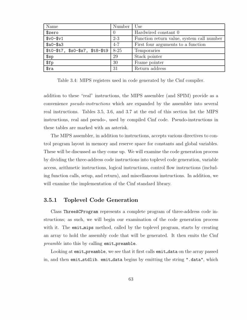
Name Number Use$zero 0 Hardwired constant 0$v0-$v1 2-3 Function return value, system call number$a0-$a3 4-7 First four arguments to a function$t0-$t7, $s0-$s7, $t8-$t9 8-25 Temporaries$sp 29 Stack pointer$fp 30 Frame pointer$ra 31 Return address
Table 3.4: MIPS registers used in code generated by the Cinf compiler.
addition to these “real” instructions, the MIPS assembler (and SPIM) provide as a
convenience pseudo-instructions which are expanded by the assembler into several
real instructions. Tables 3.5, 3.6, and 3.7 at the end of this section list the MIPS
instructions, real and pseudo-, used by compiled Cinf code. Pseudo-instructions in
these tables are marked with an asterisk.
The MIPS assembler, in addition to instructions, accepts various directives to con-
trol program layout in memory and reserve space for constants and global variables.
These will be discussed as they come up. We will examine the code generation process
by dividing the three-address code instructions into toplevel code generation, variable
access, arithmetic instructions, logical instructions, control flow instructions (includ-
ing function calls, setup, and return), and miscellaneous instructions. In addition, we
will examine the implementation of the Cinf standard library.
3.5.1 Toplevel Code Generation
Class ThreeACProgram represents a complete program of three-address code in-
structions; as such, we will begin our examination of the code generation process
with it. The emit mips method, called by the toplevel program, starts by creating
an array to hold the assembly code that will be generated. It then emits the Cinf
preamble into this by calling emit preamble.
Looking at emit preamble, we see that it first calls emit data on the array passed
in, and then emit stdlib. emit data begins by emitting the string ".data", which
63

signifies the start of the data segment to the assembler. The data segment in a
Cinf program holds global variables and constants. At this point in the compilation,
the only things remaining in the symbol table are global variables9, so the method
iterates over the list of variables in the symbol table and emits, for each, a label
(the name of the variable followed by a colon), a storage directive (the type of the
variable, and the variable’s value (the constant value for a constant, the type-defined
default value for real global variables. Since the MIPS assembler has special support
for strings, character arrays provided as string literals (between double quotes) are
emitted as string literals with the .asciiz directive. Floating-point values and arrays
of floating-point values use the .float directive; all other data uses .word. Since
small integer constants are special-cased during syntax tree construction and encoded
into immediate instructions, they require no data space.
After emitting the static data (constants and global variables) emit preamble
calls emit stdlib, which begins by emitting the string ".text", signifying the start
of the text, or code, segment, where the program itself will go. It then opens the file
backend/stdlib.s, which contains the Cinf standard library and appends it to the
array of assembly code after stripping comments (lines starting with ##). We will
examine the standard library code after discussing the rest of the code generation
process.
Finally, each 3ac instruction in the program is asked to emit code for itself into the
code array and the array is flattened, turned into a large string with lines separated
by newlines, and returned.
3.5.2 Variable Access
Cinf variables are represented as subclasses of Variable, except for small con-
stants. Since variables are (mostly) stored in memory and all of the MIPS arithmetic
and logical instructions operate on registers, there clearly needs to be some means of
uniformly loading data from and storing data back to variables, regardless of the kind
of variable. All of the Variable subclasses (and IntegerConstant, which behaves
9since each function removes its local variables and parameters from the symbol table after use.
64

like a variable) provide this interface through the load loc and store loc methods,
which take in the name of a register and generate code to load the value of the variable
into that register or store the value of that register in the variable. In addition, the
load addr method, which loads the address of a variable into a register, is provided
for indexing arrays and passing them by reference to functions. We will look at how
global variables, local variables, parameter variables, array elements, and integer con-
stants are accessed separately; for the reader wishing to follow the descriptions along
with the code, all of these classes are in the file common/symtab.rb. We have not cov-
ered these classes in detail earlier, but as they all have essentially trivial constructors
and support methods, we will look only at the load and store methods.
Global variables
Global variables and large constants reside at fixed addresses in the data segment,
each of which is labeled with the name of the variable or generated label for the
constant. As such, loading or storing data to and from a global variable is a simple
matter of adding the variable’s address (which the label provides) to the zero register
and loading the contents of memory at that address into a register with lw or storing
the contents of a register into memory at that address with sw10, which is exactly
what the load loc and store loc methods of class GlobalVariable do; the label is
stored in the instance variable @loc. Likewise, in load addr, obtaining the address of
a global variable is done by simply using the pseudo-instruction la to load the label’s
address into a register.
Local variables
Since local variables do not (and cannot, by definition) exist at fixed addresses
in memory, another mechanism besides labels is necessary to find their addresses.
That method is to store offsets into the stack frame; when space for local variables
is allocated as part of the function linearization process, each variable’s offset from
the frame pointer is stored. The frame pointer (register $fp) points to the address
10Since small values are not packed, we do not need to use load- or store-byte instructions
65
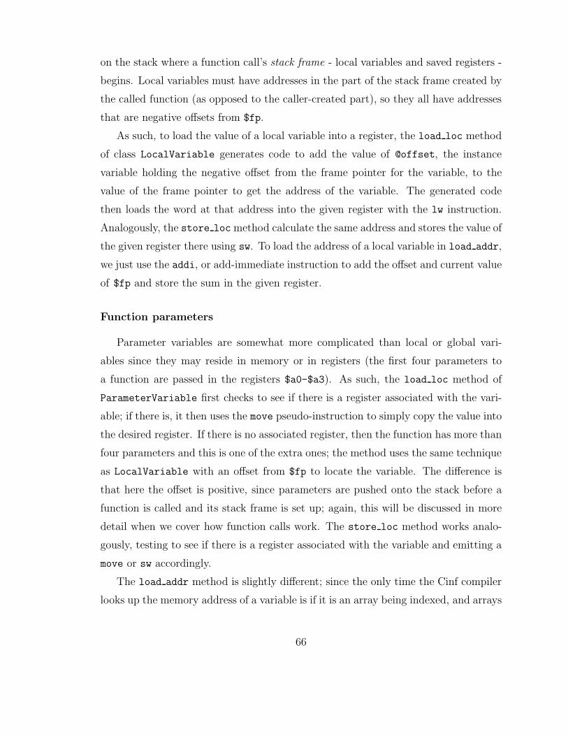
on the stack where a function call’s stack frame - local variables and saved registers -
begins. Local variables must have addresses in the part of the stack frame created by
the called function (as opposed to the caller-created part), so they all have addresses
that are negative offsets from $fp.
As such, to load the value of a local variable into a register, the load loc method
of class LocalVariable generates code to add the value of @offset, the instance
variable holding the negative offset from the frame pointer for the variable, to the
value of the frame pointer to get the address of the variable. The generated code
then loads the word at that address into the given register with the lw instruction.
Analogously, the store loc method calculate the same address and stores the value of
the given register there using sw. To load the address of a local variable in load addr,
we just use the addi, or add-immediate instruction to add the offset and current value
of $fp and store the sum in the given register.
Function parameters
Parameter variables are somewhat more complicated than local or global vari-
ables since they may reside in memory or in registers (the first four parameters to
a function are passed in the registers $a0-$a3). As such, the load loc method of
ParameterVariable first checks to see if there is a register associated with the vari-
able; if there is, it then uses the move pseudo-instruction to simply copy the value into
the desired register. If there is no associated register, then the function has more than
four parameters and this is one of the extra ones; the method uses the same technique
as LocalVariable with an offset from $fp to locate the variable. The difference is
that here the offset is positive, since parameters are pushed onto the stack before a
function is called and its stack frame is set up; again, this will be discussed in more
detail when we cover how function calls work. The store loc method works analo-
gously, testing to see if there is a register associated with the variable and emitting a
move or sw accordingly.
The load addr method is slightly different; since the only time the Cinf compiler
looks up the memory address of a variable is if it is an array being indexed, and arrays
66

are passed by reference rather than by value, if it is necessary to find the address of
a parameter variable (to index the array it points to or pass it to another function),
the necessary address is already the value of the variable. So, the method just passes
control to load loc.
Array elements
Array elements are, of course, not variables; they are part of larger variables.
They behave like variables, though, and as such it is convenient to treat them as such
in code generation. Before we proceed into the details of array element access, we
briefly note that in the constructor, we use the same type-holder trick that we did
in ArrayAccessNode for typechecking purposes; that being said, let us examine how
the class works.
The load loc method of ArrayElement begins by creating a temporary array to
append assembly code to, since indexing an array is a nontrivial operation. It then
gets the base address of the array being accessed and stores it in $s0. If the index
is a small integer constant, the method takes the value, shifts it left by two places to
multiply it by four unless the array is packed (since MIPS words are four bytes long),
and adds the resulting value to the base address of the array in $s0 with the addi
add-immediate instruction. If the index is not a small constant, the method emits
code to load its value into $s1, shifts it left by two if necessary, and uses the add
instruction to add this offset to $s0.
At this point, the address of the array element resides in $s0. If the array is
packed (i.e., a string), we use the lb load-byte instruction to load the element into
the given register; otherwise, we use the lw load-word instruction. Finally, we join the
array of generated assembly together and return the resulting string to be appended
to the greater program.
The store loc method calculates element addresses using identical logic and sim-
ply stores instead of loading, so it does not merit further attention. There is no
load addr method, as array elements can only be scalar values, not other arrays.
67
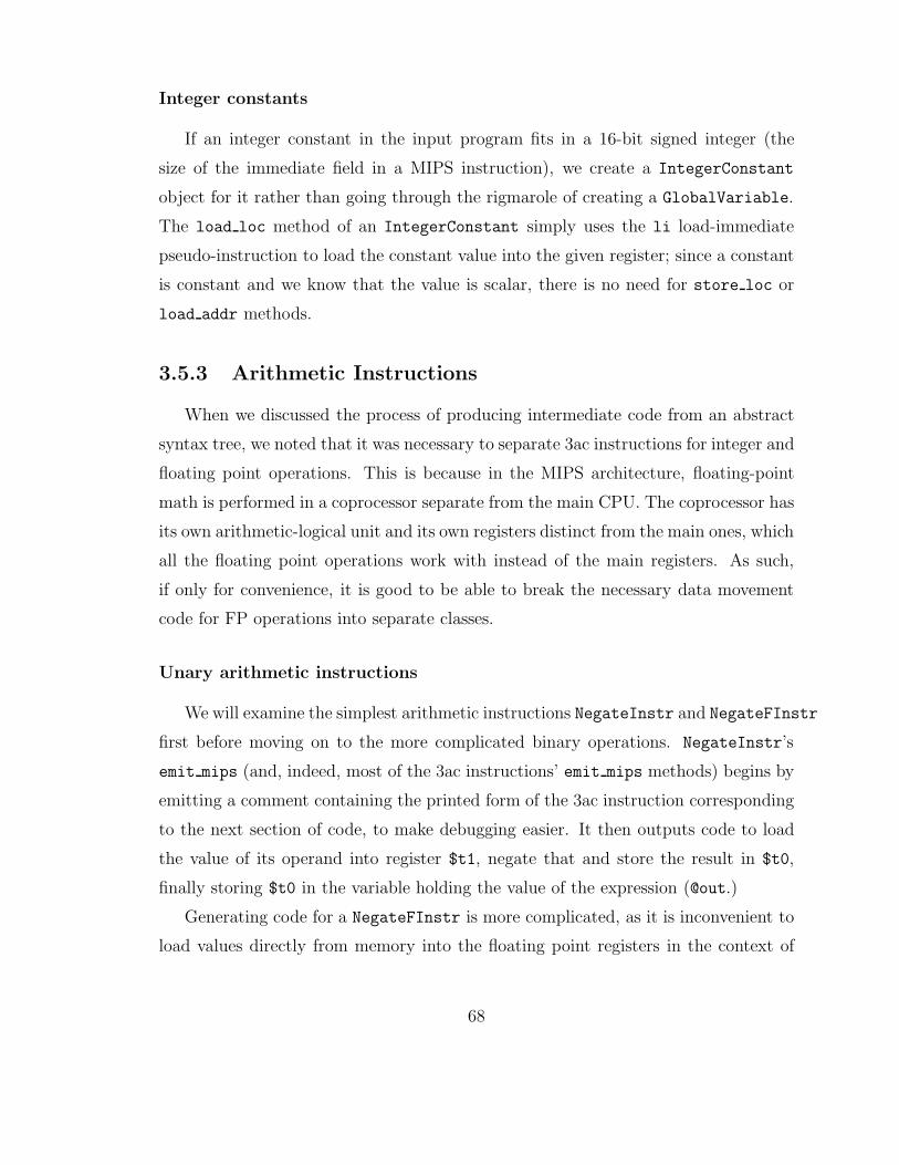
Integer constants
If an integer constant in the input program fits in a 16-bit signed integer (the
size of the immediate field in a MIPS instruction), we create a IntegerConstant
object for it rather than going through the rigmarole of creating a GlobalVariable.
The load loc method of an IntegerConstant simply uses the li load-immediate
pseudo-instruction to load the constant value into the given register; since a constant
is constant and we know that the value is scalar, there is no need for store loc or
load addr methods.
3.5.3 Arithmetic Instructions
When we discussed the process of producing intermediate code from an abstract
syntax tree, we noted that it was necessary to separate 3ac instructions for integer and
floating point operations. This is because in the MIPS architecture, floating-point
math is performed in a coprocessor separate from the main CPU. The coprocessor has
its own arithmetic-logical unit and its own registers distinct from the main ones, which
all the floating point operations work with instead of the main registers. As such,
if only for convenience, it is good to be able to break the necessary data movement
code for FP operations into separate classes.
Unary arithmetic instructions
We will examine the simplest arithmetic instructions NegateInstr and NegateFInstr
first before moving on to the more complicated binary operations. NegateInstr’s
emit mips (and, indeed, most of the 3ac instructions’ emit mips methods) begins by
emitting a comment containing the printed form of the 3ac instruction corresponding
to the next section of code, to make debugging easier. It then outputs code to load
the value of its operand into register $t1, negate that and store the result in $t0,
finally storing $t0 in the variable holding the value of the expression (@out.)
Generating code for a NegateFInstr is more complicated, as it is inconvenient to
load values directly from memory into the floating point registers in the context of
68
the mechanism that the Cinf compiler uses for variable access in generated code. As
such, the method emits code to load the variable to negate into register $t1 and move
the contents of that to floating-point register $f1. The generated code then negates
the value, putting the result in $f0, which is then moved back to $t0 and stored to
@out.
Binary arithmetic instructions
All of the 3ac instructions for binary arithmetic and logical operations are sub-
classes of BinOpNode. The emit mips method for it loads the values of the left and
right operands into $t0 and $t1 respectively before calling emit mips spec, which
is overloaded by each subclass. The code emit mips spec emits is expected to leave
its result value in $t3, the value in which is then stored into @out.
If the instruction that code is being generated for is operating on floating-point
data, a little more preparation is needed, as the floating-point instructions cannot
operate directly on the values that BinOpInstr#emit mips’s generated code left in
$t0 and $t1. As such, all the floating-point 3ac instruction classes inherit from
FloatBinOpInstr, whose emit spec method emits code to load the values in $t0 and
$t1, where the operand values are, into $f0 and $f1. It then calls emit mips fspec,
which, like emit mips spec, is overridden by every floating-point 3ac instruction to
emit code appropriate for the operation the object represents; this method is expected
to leave its result in $f3. Finally, it emits code to move the result back into integer
register $t3.
Nearly all of the integer arithmetic 3ac instructions have a simple emit mips spec
method that simply executes the appropriate instruction on $t0 and $t1, storing the
result in $t3, since addition, multiplication, subtraction, division, and remainder are
all performed by single MIPS instructions. Likewise, floating point instruction classes
all implement a one-line emit mips fspec that performs the appropriate operation
on $f0 and $f1, storing the result in $f3.
The only exceptions to this pattern are AddInstr and SubInstr. Since MIPS has
an add-immediate instruction, we can take advantage of this to generate better code
69

for the very common case of adding a small integer constant to a variable. AddInstr
and SubInstr both override emit mips to do this. If either operand is a (small
integer) constant, the generated code loads the address of the other operand and
then adds the constant to it with the addi add-immediate instruction, putting the
result in $t3 as usual; otherwise, it calls the parent class implementation, which goes
through the process described above. In the case of subtraction instead of addition,
it simply negates the constant first.
3.5.4 Logical Instructions
As with the arithmetic operations, most of the logical operations have separate
integer and floating-point flavors, for the same reason. The only exception is logical
negation, which only operates on Boolean (and therefore integer) values. The common
code between operations is factored out into a base class, as before.
Unary operators
NotInstr is the only unary logical operator. It generates code very similar to the
other unary operators: the generated code loads the value to be logically negated,
uses seq to flip it (if the value is zero, then the result will be 1; otherwise the result
will be zero), storing the result in $t3, and stores the result in @out.
Binary integer operations
All of the integer logical comparison operations use the same implementation
technique as the integer arithmetic operations: the BinOpInstr emit mips method
loads the operands into registers before calling into a specialized method on the
object. In this case, the method that eventually gets called is emit mips cond;
CondInstr, the parent class of all the binary integer logical instruction classes im-
plements emit mips spec. The implementation of emit mips spec in CondInstr is
effectively a no-op, as it just calls the appropriate emit mips cond method11. The
11In a previous iteration of the implementation of the Cinf compiler, setup code for the comparisonto be performed was emitted here. However, in the present version, no such preamble is necessary.
70

various emit mips cond methods are trivial: they use the conditional set instructions
to set $t3 to 1 if the appropriate condition is true and 0 if it is false.
Binary floating-point operations
The floating-point comparison instructions are more complicated than their inte-
ger counterparts, both for the usual reason and because the floating point comparison
instructions set a bit in the floating-point coprocessor status flags instead of operat-
ing on a register. The status flags are not accessible directly as a register, but it is
possible to either branch conditionally based on their status or, more interestingly,
move data conditionally.
All of the floating point instructions are subclasses of FloatCondInstr, whose
emit mips cond does all the heavy lifting - the subclass constructors merely pass the
mnemonic for the instruction to its constructor, and it performs the code generation.
The emit mips cond method starts in the usual FP instruction fashion, emitting the
code to load the values in $t0 and $t1 into $f0 and $f1. The generated code then
performs the appropriate comparison and loads the literal value 1 into $t3. If the
comparison was true, then 1 (true) will be the result of the expression; otherwise, the
conditional move instruction movf will set $t3 to 0 (false).
3.5.5 Control Flow Instructions
The control flow instructions can be roughly divided into jumps (conditional and
unconditional) and function call, setup, and return code. We will examine the two
classes separately.
Jump instructions
There are two kinds of jump instructions in the three-address code used by the
Cinf compiler: conditional and unconditional. Both jumps target labels, so we will
discuss labels first, and then the two kinds of jump.
Emitting code for a LabelInstr is trivial: the assembly for a label is just the
name of the label followed by a colon; as such, the emit mips method for this class is
71
trivial. A GlobalLabelInstr adds a .globl declaration for the label to the emitted
label; global labels are used for the names of functions so that breakpoints may be
set at them when debugging.
A JumpInstr is a simple unconditional jump, so one might expect the emitted
assembly code to be simple, and one would be correct. The emit mips method simply
emits a MIPS unconditional jump instruction (j) targeting the given label.
Finally, the code generated for a BranchFalseInstr will simply load the value of
the given operand and compare it against the zero register (recall that the integer
zero is false in Cinf). If they are equal, it will branch to the given label.
Function call and return instructions
The code generation process for function call, setup, and return instructions is
probably the most subtle and complicated part of the entire compiler backend. We
will examine it in three parts: the function call code, the function prologue, and the
return instruction.
The process of generating code for a function call begins with the emit mips
method of class ArgListPushInstr. As one might guess from the name of the class,
this method pushes any arguments for the function onto the stack and sets up the
caller part of the stack frame, as seen in 3.4. It begins by calculating the amount
that the stack pointer will have to be adjusted by. First, obviously, space needs to be
reserved for the frame pointer, as the called function requires its own frame, that is
one word, or four bytes. Next, space must be reserved for each of the arguments being
passed to the function, so we multiply the size of the list of arguments by four; this
works because all the primitive types are stored in words and arrays are passed by
reference. Finally, we calculate the number of words on the stack that will be needed
to save the current contents of the argument registers, since the current function or
a function farther up the call stack may be using them; this will be anywhere from
0 to 4 depending on how many arguments the function takes. So, the total amount
of space needed on the stack will be number of words for parameters (amt) plus the
number of words for saved registers (saveregs) plus one word for the frame pointer.
72
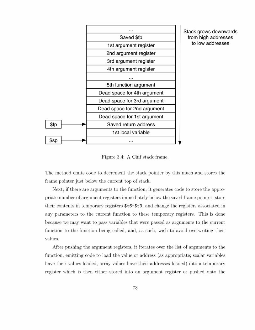
4th argument register
...
5th function argument
Dead space for 4th argument
Dead space for 3rd argument
Dead space for 2nd argument
Dead space for 1st argument
Saved return address
1st local variable
...
$fp
$sp
3rd argument register
1st argument register
Saved $fp
2nd argument register
... Stack grows downwardsfrom high addresses
to low addresses
Figure 3.4: A Cinf stack frame.
The method emits code to decrement the stack pointer by this much and stores the
frame pointer just below the current top of stack.
Next, if there are arguments to the function, it generates code to store the appro-
priate number of argument registers immediately below the saved frame pointer, store
their contents in temporary registers $t6-$t9, and change the registers associated in
any parameters to the current function to these temporary registers. This is done
because we may want to pass variables that were passed as arguments to the current
function to the function being called, and, as such, wish to avoid overwriting their
values.
After pushing the argument registers, it iterates over the list of arguments to the
function, emitting code to load the value or address (as appropriate; scalar variables
have their values loaded, array values have their addresses loaded) into a temporary
register which is then either stored into an argument register or pushed onto the
73
stack. Note that four “dead slots” are left on the stack for the first four arguments;
this makes accessing the fifth, sixth, etc. parameters easier. At this point, the job
is finished in terms of setting up the stack frame, and we will proceed to look at
the beginning of the code emitted for a CallInstr. The first code emitted from
emit mips in CallInstr is a jal or jump-and-link instruction; this jumps to the
code at the given label and stores the address of the next instruction in register $ra.
We will temporarily leave CallInstr to look at stack frame setup from the callee’s
side.
The first 3ac instruction in a Cinf function is the PrologInstr, which is the
function prologue. which sets up the callee part of the stack frame. The emitted code
for this instruction sets up the initial frame pointer as being one word below the old
top of stack, moves the stack pointer @nlocals words below the frame pointer, and
stores the old return address at the address pointed to by the frame pointer. The
advantage of having the frame pointer be set up like this is that now, assuming for now
that all local variables are scalar, the first local variable is at $fp-4, the second is at
$fp-8, and so on, which makes the math involved in calculating addresses somewhat
simpler. Likewise, the fifth (since the first four parameters are passed in registers)
parameter is $fp+20, the sixth is $fp+24, and so on. Non-scalar parameters are, of
course, handled properly; @nlocals is the total number of bytes needed to be reserved
on the stack for the function’s local variables, scalar or otherwise. It was calculated
during intermediate code generation.
After the stack frame for a function has been set up, the function goes about its
normal execution until it hits a ReturnInstr instruction. The generated code for this
first loads the value of the expression being returned, if any, into $v0 which is, by
convention, where return values are placed. It then pops all of the local variables off
the stack by bringing $sp up to $fp, loads the return address from the word pointed
to by $fp, and pops the word that held that off the stack; at this point, the stack is
exactly as the code generated in ArgListPushInstr left it. Finally, it uses the jr, or
jump-register instruction to jump to the return address.
We return to CallInstr#emit mips at this point, as the code emitted after the
jal is code to clean up after the function. First, it again calculates the amount
74

of stack space that was used in setting up the caller part of the stack frame in
ArgListPushInstr. It then emits code to restore any argument registers that were
saved, setting the associated registers of any parameters of the current function back
to the appropriate registers. Finally, the generated code restores the frame pointer
from where it had been saved on the stack, restores the stack pointer by popping the
caller part of the stack frame off, and saves the return value in $v0 into out as usual,
unless the function was void.
3.5.6 The Standard Library
The Cinf standard library functions are mostly wrappers around the SPIM system
calls listed in table 3.8[11]. A system call is performed by putting the system call
number in $v0 and any arguments in the registers appropriate to that call; the result,
if any, is placed in $v0. The two that are not, the integer-float and float-integer
conversion functions, are simple wrappers around single MIPS instructions.
We will look briefly at the standard library functions in the order which they
are defined in backend/stdlib.s. The first five functions, print int, read int,
print string, print float, and read float are trivial, since the Cinf calling con-
vention coincides with the system call convention. The print syscalls take their
arguments in $a0, where the function call setup code put them as described above,
and the read calls put the read value in $v0, where the post-function call cleanup
code expects to find it.
The next function, read string, is unfortunately more complicated, not for rea-
sons related to calling convention, but because the semantics of the SPIM read string
system call are undesirable; it takes in a buffer holding up to n characters and reads
at most n-1 characters and a trailing newline into it. We do not desire all of our
user-provided strings to have a trailing newline, so we loop through the string and
strip it off if it exists.
SPIM system calls for reading and printing characters exist, and so we use them
to implement reading and displaying characters. read char loads the appropriate
system call number into $v0, performs the system call, and returns; since the read
75
character is left in $v0, which is where the Cinf calling convention expects return
values to be left, no further code is necessary. print char is equally simple, since it
expects the character to be printed to be in $a0, which is where the calling function
places the first argument to a function under the Cinf calling convention.
Likewise in print char, we get a word of scratch space, store the character to be
printed in that word, and null-terminate it. We then load $a0 with the address of the
buffer, load $v0 with the appropriate system call number, and perform the syscall.
Finally, we pop the scratch space and return.
Finally, we look at the nearly-identical inttofloat and floattoint functions.
Both load a passed-in value into a floating-point register, operate on it, store the
result back into $v0, and return; the former uses the cvt.s.w instruction, which
converts an integer to a floating-point number, and the latter uses cvt.w.s, which
rounds a floating-point number to an integer.
76
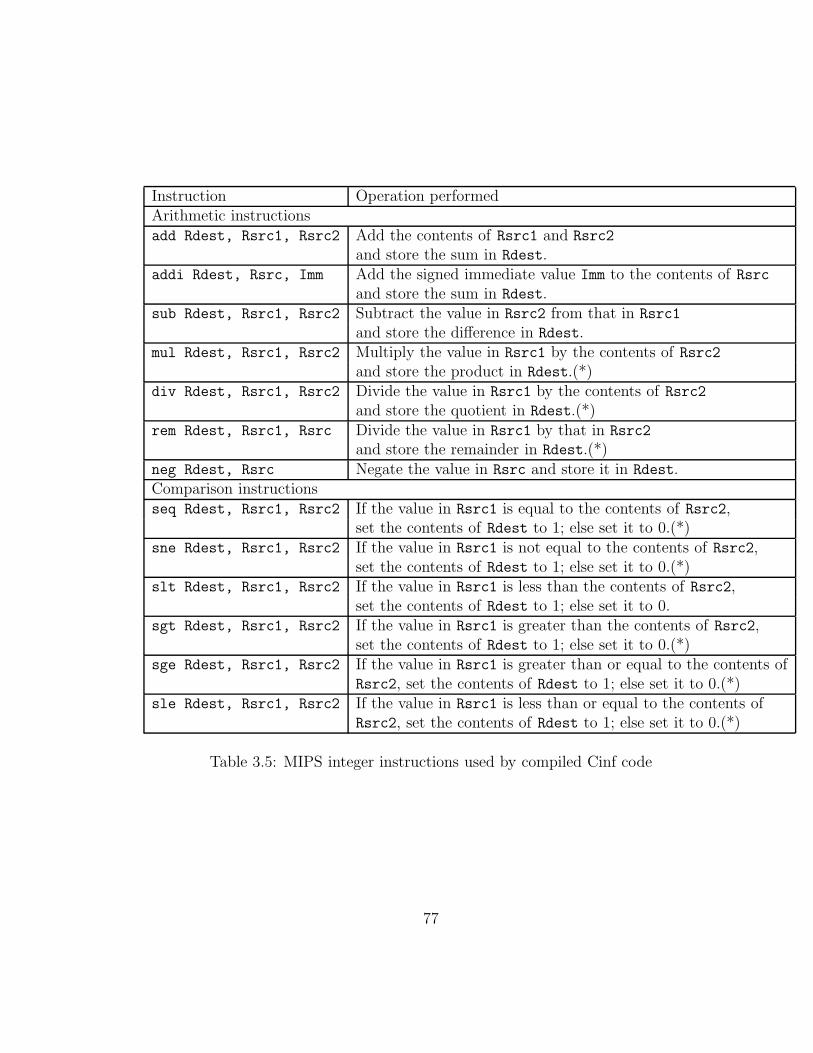
Instruction Operation performedArithmetic instructionsadd Rdest, Rsrc1, Rsrc2 Add the contents of Rsrc1 and Rsrc2
and store the sum in Rdest.addi Rdest, Rsrc, Imm Add the signed immediate value Imm to the contents of Rsrc
and store the sum in Rdest.sub Rdest, Rsrc1, Rsrc2 Subtract the value in Rsrc2 from that in Rsrc1
and store the difference in Rdest.mul Rdest, Rsrc1, Rsrc2 Multiply the value in Rsrc1 by the contents of Rsrc2
and store the product in Rdest.(*)div Rdest, Rsrc1, Rsrc2 Divide the value in Rsrc1 by the contents of Rsrc2
and store the quotient in Rdest.(*)rem Rdest, Rsrc1, Rsrc Divide the value in Rsrc1 by that in Rsrc2
and store the remainder in Rdest.(*)neg Rdest, Rsrc Negate the value in Rsrc and store it in Rdest.Comparison instructionsseq Rdest, Rsrc1, Rsrc2 If the value in Rsrc1 is equal to the contents of Rsrc2,
set the contents of Rdest to 1; else set it to 0.(*)sne Rdest, Rsrc1, Rsrc2 If the value in Rsrc1 is not equal to the contents of Rsrc2,
set the contents of Rdest to 1; else set it to 0.(*)slt Rdest, Rsrc1, Rsrc2 If the value in Rsrc1 is less than the contents of Rsrc2,
set the contents of Rdest to 1; else set it to 0.sgt Rdest, Rsrc1, Rsrc2 If the value in Rsrc1 is greater than the contents of Rsrc2,
set the contents of Rdest to 1; else set it to 0.(*)sge Rdest, Rsrc1, Rsrc2 If the value in Rsrc1 is greater than or equal to the contents of
Rsrc2, set the contents of Rdest to 1; else set it to 0.(*)sle Rdest, Rsrc1, Rsrc2 If the value in Rsrc1 is less than or equal to the contents of
Rsrc2, set the contents of Rdest to 1; else set it to 0.(*)
Table 3.5: MIPS integer instructions used by compiled Cinf code
77

Instruction Operation performedJump and branch instructionsbeq Rsrc1, Rsrc2, lbl If the value in Rsrc1 is equal to the contents of Rsrc2,
jump to the code at label lbl.j lbl Unconditionally jump to the code at label lbl.jr Rsrc Unconditionally jump to the code at the address in Rsrc.jal lbl Unconditionally jump to the code at label lbl.
Store the address of the next instruction in $ra.syscall Call into the operating system to perform a privileged operation.Data movement instructionslw Rdest, Imm(Rsrc) Add the immediate value Imm to the contents of Rsrc to
obtain an address; load the contents of the word in memoryat that address into Rdest.
sw Rdest, Imm(Rsrc) Add the immediate value Imm to the contents of Rsrc toobtain an address; store the contents of Rdest intothe word in memory at that address.
lb Rdest, Imm(Rsrc) Add the immediate value Imm to the contents of Rsrc toobtain an address; load the zero-extended value of the bytein memory at that address into Rdest.
sw Rdest, Imm(Rsrc) Add the immediate value Imm to the contents of Rsrc toobtain an address; store the contents of the low byte of Rdestinto the byte in memory at that address.
la Rdest, lbl Load the memory address that lbl refers to into Rdest.li Rdest, Imm Load the immediate value Imm into Rdest.move Rdest, Rsrc Store the contents of Rsrc in Rdest. (*)
Table 3.6: MIPS control and integer data movement instructions
78

Instruction Operation performedArithmetic instructionsadd.s FRdest, FRsrc1, FRsrc2 Add the contents of FRsrc1 and FRsrc2
and store the sum in FRdest.sub.s FRdest, FRsrc1, FRsrc2 Add the contents of FRsrc1 and FRsrc2
and store the difference in FRdest.mul.s FRdest, FRsrc1, FRsrc2 Multiply the contents of FRsrc1 and FRsrc2
and store the product in FRdest.div.s FRdest, FRsrc1, FRsrc2 Divide the contents of FRsrc1 and FRsrc2
and store the result in FRdest.neg.s FRdest, FRsrc Negate the value in FRsrc and store it in FRdest.Comparison instructionsc.eq.s FRsrc1, FRsrc2 Set the FP condition flag if the value in FRsrc1
equals that in FRsrc2.c.ne.s FRsrc1, FRsrc2 Set the FP condition flag if the value in FRsrc1
does not equal that in FRsrc2.c.lt.s FRsrc1, FRsrc2 Set the FP condition flag if the value in FRsrc1
is less than that in FRsrc2.c.gt.s FRsrc1, FRsrc2 Set the FP condition flag if the value in FRsrc1
is greater than that in FRsrc2.c.le.s FRsrc1, FRsrc2 Set the FP condition flag if the value in FRsrc1
is greater than or equal to that in FRsrc2.c.le.s FRsrc1, FRsrc2 Set the FP condition flag if the value in FRsrc1
is less than or equal to that in FRsrc2.Data conversion instructionscvt.s.w FRdest, FRsrc Convert the integer value in FRsrc to
a floating-point value and store the result in FRdest.cvt.w.s FRdest, FRsrc Convert the floating-point value in FRsrc to
an integer value and store the result in FRdest.Data movement instructionsmtc1 Rsrc, FRdest Move the contents of general-purpose register Rsrc to
FP register FRdest.mfc1 Rdest, FRsrc Move the contents of FP register FRsrc to
general-purpose register Rdest.movf Rdest, Rsrc, Imm Move the contents of GPR Rsrc to Rdest
if bit Imm of the FP condition word is unset
Table 3.7: MIPS floating point instructions.
79

Service Number Arguments Resultprint int 1 $a0 = an integerprint float 2 $f12 = a floatprint string 4 $a0 = a stringread int 5 an integer in $v0
read float 6 a float in $f0
read string 8 $a0 = address of a buffer$a1 = length of buffer
Table 3.8: SPIM system calls used by the Cinf standard library
80
Chapter 4
Conclusion
4.1 Summary
The object of this work was to demonstrate that modern advances in theoretical
computer science can be married to traditional mainstream programming languages
to produce tools that make programming easier without requiring programmers to
become familiar with a fundamentally different paradigm of computing. This goal
has definitely been achieved; the result of a year’s effort was a fully functioning
compiler for a language very similar those in the popular C family with a type system
inspired by those of functional languages that fundamentally reduces the number of
type declarations and other such annotations required in a program while retaining
the safety of static typing. The language, as it stands, is perfectly usable for writing
programs that perform real tasks. However, it was deliberately limited in both design
and implementation in order to make it possible to complete in the allotted time and
is missing a number of features, both in terms of the design of the language and
the implementation, that a working programmer would desire. In this last and final
section we will discuss some of these limitations and suggest extensions to make the
language more usable, as well as discussing some of the lessons learned in the process
of completing the work.
81
4.2 Possible Improvements
4.2.1 Language Improvements
Polymorphic functions
Cinf frees the programmer from the burden of type declarations like Hindley-
Milner typed languages do, but it is in many ways as limited as C, the language it most
closely resembles. As discussed in the introduction to this work, one of the biggest
advantage of Hindley-Milner typing is not the lack of reliance on type annotations
but on its ability to make code generic through polymorphism. Programs in HM-
typed languages can be generic, capable of operating on data of many types, without
requiring the cumbersome annotations of templates or generics as seen in C++ and
Java. Cinf or a language like it could be extended to have this capability through the
addition of a much more advanced type inference engine and type checker.
User-defined types
One of the biggest shortcomings of Cinf is that it does not allow the program-
mer to define types besides arrays of primitive types. Most imperative languages
allow the programmer to define structures, which are collections of data of different
types. Languages in the ML family have highly sophisticated type definition mech-
anisms. Both imperative and functional languages allow these types to be recursive,
or containing values which are themselves of the type being defined; for example,
linked lists and trees. The ability to create and manipulate recursive data is essential
to solving many common problems, and as such, the addition of a type definition
mechanism supporting recursive types would be a great improvement to Cinf. In ad-
dition to the implementation details associated with representing and manipulating
more complex data, the type inference engine and type checker would have to be
extended to be much more powerful, because the ability to define recursive types (es-
pecially when combined with polymorphic functions) complicates the type inference
and checking code in a compiler greatly (though it does not affect the generated code
and has no penalty at run-time). It would be necessary to essentially re-implement
82
the Hindley-Milner system and possibly extend it to be more friendly towards imper-
ative languages; the interested reader is invited to look at [12] and [13] for a much
more thorough and detailed explanation of type theory than that provided in these
pages.
References
It is often desirable to be able to pass a reference to a variable to a function instead
of its value so that changing the value of the argument variable in the called function
changes the value of the variable in the calling function. In addition, references are
essential for using data structures whose size cannot be determined at compile time,
such as complex data structures. However, the implementation of advanced type
systems in languages with mutable references is still an active area of research1 with
open problems; it seems, therefore, that it would be a very difficult problem to extend
Cinf’s type system to make mutable references safe. In addition, adding support for
references to the Cinf compiler would not be an easy task.
First-class functions
Having functions be first-class entities that can be passed as arguments to other
functions, stored, and called indirectly is a feature of immense power, one which
all major functional languages provide and some imperative languages implement
in some form. In addition to the ability to pass around references to already de-
fined functions present in most imperative languages, functional languages (and a
few newer imperative ones) add the ability to create functions on the fly, as needed.
These “anonymous functions”, called closures2, are powerful and useful, and would
be a desirable addition to the mainstream programmer’s toolkit; moreover, they are
handily covered by Hindley-Milner-style typing. The work required to add support
for first-class functions to Cinf’s type system, while again complex, would be within
the realm of possibility. However, the work to add support for creating and manip-
1Some of this work can be seen in [13].2Closures are named as such because they “close over” the scope that they are defined in - that
is, they hold onto the variables present in that scope, even after that scope has been exited.
83

ulating closures would be difficult, as it would entail substantially changing the Cinf
runtime model and adding garbage collection.
Object-Orientation
Many popular imperative languages today support object-orientation, a model of
programming which is based around the idea of, instead of having functions that
operate on data, inverting the relation and giving data behavior.The object-oriented
model has been a runaway success since it became mainstream with C++, and shows
no signs of going away, so it might well be a good idea to add support for object
orientation to Cinf or a Cinf-like language. The technical challenges in adapting a
procedural language like Cinf to be object oriented, just in terms of representation
and access details, are far beyond the scope of this work, and are quite difficult;
however, as with first-class functions, the necessary changes would largely be limited
to the type inference and checking code and would again have no run-time penalty.
In addition, the interaction of object-orientation (which traditionally has been a very
dynamic model of programming) with advanced static typing is still a wide-open area
of research3, and many details of the semantics of such a synthesis remain unknown.
Of the possible language extensions listed here, this is far and away the least feasible.
4.2.2 Implementation Improvements
The language improvements discussed in the previous section would require deep
and far-reaching changes to the language and implementation, possibly to the point
where it would not resemble its current state closely, if at all. In this section, we will
set our sights considerably lower and examine more incremental improvements to the
existing implementation of the language.
Register allocation
The biggest improvement that could be made to the existing Cinf compiler would
be to add register allocation to the code generation stage. Register allocation is
3Again, [13] is an excellent survey of recent developments in type theory.
84

the process of assigning CPU registers to local variables so that they are easily and
quickly accessible without having to refer to memory every time a variable is used.
MIPS has 32 registers, but the Cinf compiler only makes use of a handful of them
for temporaries in expression evaluation and argument-passing. Register allocation
is a difficult problem; in fact, according to [1], it is NP-complete in the worst case.
However, there is a well-known algorithm4 that works in reasonable time for the vast
majority of programs. This change would immensely improve the quality and speed
of the generated code.
Separate compilation
As it stands, a Cinf program must be one file. This obviously limits the maximum
size of programs in the language, as very large source files are unwieldy. Adding
support for compiling multiple source files and linking them together to form a com-
plete program would be relatively straightforward, with the major subtleties arising
in ensuring that global variable and function names do not conflict. In addition to
this, it would be very desirable to add support for putting declarations of functions
and global variables in files which could be included by other files; this, when com-
bined with separate compilation, would make it possible to put together libraries of
common routines in Cinf. It would also remove the current necessity of editing the
file tree/stdlib.rb whenever the standard library is modified.
Alternate immediate representations
The intermediate representation that the Cinf compiler uses, three-address code, is
a very old style of intermediate code. In recent years, newer intermediate representa-
tions, such as static single-assignment form, have become prominent, becoming used
in popular compilers like GCC, the GNU Compiler Collection. SSA form is a variation
of three-address code in which each variable in the generated code is assigned to only
once. The discrepancies which arise from variables being assigned to conditionally
(e.g. set one way in the body of an if statement and another in its else clause) are
4The algorithm is discussed in [1]
85

resolved using objects called φ-functions[2]. SSA form is popular because it is much
easier to optimize than 3ac; furthermore, it is only moderately harder to generate
SSA-form code from syntax trees and assembly code from SSA-form code. Adapting
the Cinf compiler to use SSA form instead of 3ac for the intermediate representation
of a program would be a nontrivial, but definitely achievable, project.
Optimization
The Cinf compiler as presented in this work does very little in the way of opti-
mization; folding of constant expressions and small integer expressions is essentially
the only thing the compiler does to improve input code. A full discussion of code
optimization is far beyond the scope of this section; the interested reader is, as usual,
referred to [1]. Depending on the scope and number of desired optimizations, extend-
ing the Cinf compiler to optimize code could be a project of difficulty ranging from
moderate to very hard.
Porting the compiler
Currently, the output of the Cinf compiler is MIPS assembly code that runs on
the SPIM simulator. It might be desirable to port the compiler to generate assembly
code for a real machine, so that its output could be run without requiring a simulator.
Depending on the target architecture, the difficulty for this would range from nearly
trivial (if we wish to make the output code run on a real MIPS machine, it would only
be necessary to fix up the standard library functions to use that platform’s system
call convention) to difficult (porting the compiler to the Intel IA32 architecture used
in today’s PCs, which is fundamentally different from MIPS in many ways, would be
a serious project).
4.3 Lessons
Designing a new programming language and building a fully functional compiler
for it that produces assembly language is one of the most complicated and broad tasks
86

in practical computer science, spanning the fields of programming languages, ma-
chine architecture, formal language theory, algorithms, and software engineering[1].
It would be strange if no lessons were learned from such an undertaking, and, indeed,
the process has proved to be quite a learning experience.
The most important lesson learned in the process of the work was undoubtedly
the importance of scheduling. The plan that was made early on in the process was,
unfortunately, not adhered to remotely as well as it should have been, leading to a
storm of last-minute work. Furthermore, had many of the deadlines on the original
plan not been missed, the final implementation of the compiler would have been
considerably easier, as many of the milestones on the schedule were programs related
to the compiler, such as the planned Cinf interpreter that was never written. Should
the author undertake such a work again, he would endeavor to hew much more closely
to the schedule, and to keep the schedule constantly updated to match reality.
A second lesson learned was the importance of planning and design. A specifica-
tion for the language (Chapter 1) existed relatively early in the process; implemen-
tations of the language could be compared for features and behavior against those
documented in the spec. However, no such detailed plan existed for the various inter-
nal details of the compiler. If time had been taken to actually work out the details of
what syntax trees should look like, what the intermediate representation should look
like, and what the type inference algorithm should be, the implementation process
would have gone much more smoothly.
Finally, in addition the “soft” lessons listed above, two invaluable “hard,” or
technical lessons came out of this project. The first is that many difficult problems
can be solved by adding sufficient layers of indirection - that is, by manipulating
references to data instead of the data objects themselves. Solving problems through
appropriate indirection was a constant theme in the construction of the Cinf compiler
- the most obvious example is the use of TypeHolders to enable propagation of type
information across the syntax tree. The second is that laziness is a virtue; that is, not
laziness as in letting the project fall behind schedule, but laziness in code, putting
off actually performing an action as long as possible. The obvious example in the
compiler was deferring allocation of local variables until after it was determined how
87

many temporaries would be needed, but there are other instances.
4.4 Looking Forward
Cinf is now a finished project, as far as the author is concerned. The implemen-
tation of the language is provided under a liberal license that allows curious readers
to experiment with, modify, and redistribute it. It is hoped that it will provide in-
spiration, if not hard code, to language designers working to bring advanced features
to mainstream languages and thereby make the lives of working programmers that
much easier.
Mainstream languages must progress. We are entering an era of computing in
which the old paradigm, in which the speed of processors doubles every eighteen
months[11], no longer applies and in which programmers must instead turn to more
clever algorithms and parallel processing to increase performance. More elaborate
algorithms are generally easier to implement with more expressive languages, and
threads or other means of achieving parallelism are exceedingly difficult to deal with
without language support. The demand for new software and new kinds of software is
not going away, and so mainstream languages must progress to tackle these new prob-
lems. To paraphrase David Hilbert’s famous words, as programmers and language
designers, we can advance, and we must advance.
88

Bibliography
1. Alfred V. Aho, Ravi Sethi, and Jeffrey D. Ullman. Compilers: Principles, Tech-
niques, and Tools. Addison-Wesley, 1986.
2. Andrew W. Appel. Modern Compiler Implementation in Java. Cambridge Uni-
versity Press, 2002.
3. Henk Barendregt. The lambda calculus, its syntax and semantics. North-Holland,
1984.
4. Luca Cardelli. Basic polymorphic typechecking. Science of Computer Program-
ming, 8(2), 1987.
5. Pascal Manoury Chailloux, Emmanuel and Bruno Pagano. Developing Applica-
tions with Objective Caml. O’Reilly France, 2000.
6. Jutta Degener. ANSI C Yacc Grammar.
http://www.lysator.liu.se/c/ANSI-C-grammar-y.html, 1995.
7. Brian W. Kernighan and Dennis M. Ritchie. The C Programming Language.
Prentice Hall, 1988.
8. Donald Knuth. The Art of Computer Programming, Volume 1: Fundamental
Algorithms. Addison-Wesley, 1997.
9. Kenenth C. Louden. Programming Languages: Principles and Practice.
Brooks/Cole-Thomson Learning, 2003.
89
10. John McCarthy. Recursive functions of symbolic expressions and their computa-
tion by machine. Communications of the ACM, 3(4):26–60, 1960.
11. David A. Patterson and John L. Hennessy. Computer Organization and Design:
The Hardware/Software Interface. Elsevier, 2005.
12. Benjamin C. Pierce. Types and Programming Languages. MIT Press, 2002.
13. Benjamin C. Pierce. Advanced Topics in Types and Programming Languages.
MIT Press, 2004.
14. Dave Thomas, Chad Fowler, and Andy Hunt. Programming Ruby: The Pragmatic
Programmers’ Guide, Second Edition. The Pragmatic Bookshelf, 2005.
90
Appendix A
Sample Code
The following pages show two simple Cinf programs in source and compiled forms.
The program exp.cinf takes in two numbers and prints the result of computing
the first raised to the second recursively. The compiler output is in exp.s.
The program f2c.cinf prompts the user for a temperature in degrees Fahrenheit,
prints the result of converting the supplied temperature to degrees Celsius, and asks
if the user wishes to convert more temperatures. If so, it loops back to the beginning;
otherwise, it exits. The compiler output is in f2c.s.
The compiled output is interspersed with comments showing what three-address
code instruction was translated to the MIPS assembly code immediately following it.
Both files are prefaced by the standard library functions.
91

Appendix B
The Implementation
This appendix contains the complete source code for the Cinf compiler along with
instructions for building and using it. The entire distribution may also be found
online at http://www.simons-rock.edu/∼adam/cinf.tar; this includes both the
contents of this appendix and the two sample Cinf programs in the previous one.
The Cinf compiler and sample programs are provided under the terms of the
MIT/X11 license, the terms of which may be found in the file LICENSE.TXT in the
source distribution.
104