diplomarbeit - infoscience · diplomarbeit zum thema simulation of the welding process of steel...
TRANSCRIPT

Diplomarbeit
zum Thema
Simulation of the welding process of steel tube joints made of S355
and S690
vorgelegt von: cand. ing.
Janna Krummenacker
Erstprüfer: Univ.-Prof. Dr.-Ing. T. Ummenhofer
Zweitprüfer: Univ.-Prof. Dr.-Ing. H. Blass
April 2011

Preface
This diploma thesis has been carried out during an Erasmus exchange at the Steel StructuresLaboratory (ICOM) at the École Polytechnique Fédérale de Lausanne (EPFL).
First, I would like to thank my supervisor Professor Thomas Ummenhofer who supportedthe idea of an exchange and initiated the contact with Professor Alain Nussbaumer, whomI would like to thank for his continuos and highly qualified support. The regular meetingsand his questions always helped me very much to progress with my work. I would also like toexpress my sincere gratitude to Farshid Zamiri for his dedicated mentoring and competendassistance with all my questions. Thank you very much to Claire Acevedo, whose experiencein the field of welding simulation and advice was very helpful and simplified the start of mywork a lot. I also would like to thank the entire ICOM staff for their cordial welcome.
Thank you to Professor Andreas Mortensen and the Laboratory of Mechanical Metallurgy(LMM) for the provision of the tensile testing machine. I also would like to thank WillyDufour and Gilles Guignet for their assistance and help during the set-up of the machine andthe experiments.
Lastly, I would like to thank my friend Mariette Martin for the great and time-consumingediting of my work.

Abstract
Welding is an important joining method for the work with metals. During the welding process,the material is heated and deforms plastically which leads a change in microstructure in theheat affected zone, to complex residual stress distributions, and distorsions. The residualstresses can have a major impact, among other phenomena, on the fatigue resistance of awelded structure. The aim of this work was to develop a model with the finite element softwareAbaqus for the simulation of a welding process for butt welded tubes and the calculation ofthe resulting welding residual stress field.
The residual stress field depends on several input parameters, like the geometry, the heatinput, the welding speed, the material data, and the number of weld passes. The chosendimensions of the tubes are realistic for tubular steel bridge constructions. Since, no exper-imental welding procedures were conducted, the welding parameters like the heat input andthe welding speed were estimated in order to obtain a realistic temperature distribution in theweld and the heat affected zone. The assignment asked to place a main focus on the influenceof the material data and the number of weld passes.
Within the framework of this work, tensile tests at three different temperatures wereconducted in order to find the deformational behavior of the two different steel grades S355and S690. The results show generally good agreement with the data given by the EuropeanStandard for the structural fire design of steel structures [11], that is noted Eurocode 3(EC3) in the course of this work. According to the test results, the yield strength at roomtemperature are underestimated by the Eurocode 3.
Based on the experiments and the data given in the Eurocode 3, the influence of themechanical properties were studied in several Abaqus models. For the description of thetemperature dependent material behavior, a bilinear stress-strain curve was implemented.The resulting stress distributions show a similar trend, but the offset values between thestress curves of two models are dependent on the position in circumferential direction and thedistance in axial direction. During the literature study, different welding simulation programswere compared. With specific welding simulation programs, mostly two-dimensional modelscan be realised. A major advantage of these programs is, that phase transformations can easilybe considered and therefore a more realistic material model can be implemented provided thatthe temperature dependant behavior of the different microstructural phases are known.
The influence of the number of weld passes was studied by comparing a single- and a multi-pass model with the material data from the Eurocode 3. The total heat input and the weldingspeed was the same for all the models. The tendency of the resulting stress distributions variedgreatly and therefore implies that a multi-pass model cannot be approximated by a singlepassmodel.
Contents
1 Introduction 8
2 State of knowledge 102.1 Welding temperature field . . . . . . . . . . . . . . . . . . . . . . . . . . . . . 102.2 Residual stresses . . . . . . . . . . . . . . . . . . . . . . . . . . . . . . . . . . 11
2.2.1 Welding residual stresses . . . . . . . . . . . . . . . . . . . . . . . . . . 122.3 Material properties . . . . . . . . . . . . . . . . . . . . . . . . . . . . . . . . . 122.4 Numerical simulation . . . . . . . . . . . . . . . . . . . . . . . . . . . . . . . . 13
2.4.1 Thermal modeling and simulation . . . . . . . . . . . . . . . . . . . . . 142.4.2 Simulation programs . . . . . . . . . . . . . . . . . . . . . . . . . . . . 15
3 Experiments 163.1 Specimen geometry . . . . . . . . . . . . . . . . . . . . . . . . . . . . . . . . . 163.2 Performance of the tests . . . . . . . . . . . . . . . . . . . . . . . . . . . . . . 173.3 Results . . . . . . . . . . . . . . . . . . . . . . . . . . . . . . . . . . . . . . . . 19
3.3.1 Steel type S355 . . . . . . . . . . . . . . . . . . . . . . . . . . . . . . . 193.3.2 Steel type S690 . . . . . . . . . . . . . . . . . . . . . . . . . . . . . . . 21
4 Numerical simulation 254.1 Thermal analysis . . . . . . . . . . . . . . . . . . . . . . . . . . . . . . . . . . 25
4.1.1 Theory . . . . . . . . . . . . . . . . . . . . . . . . . . . . . . . . . . . . 254.1.2 Finite Element solution . . . . . . . . . . . . . . . . . . . . . . . . . . 274.1.3 Heat source . . . . . . . . . . . . . . . . . . . . . . . . . . . . . . . . . 294.1.4 Thermal material properties . . . . . . . . . . . . . . . . . . . . . . . . 304.1.5 Boundary conditions . . . . . . . . . . . . . . . . . . . . . . . . . . . . 31
4.2 Mechanical analysis . . . . . . . . . . . . . . . . . . . . . . . . . . . . . . . . . 334.2.1 Theory . . . . . . . . . . . . . . . . . . . . . . . . . . . . . . . . . . . . 334.2.2 Mechanical material properties . . . . . . . . . . . . . . . . . . . . . . 354.2.3 Boundary conditions . . . . . . . . . . . . . . . . . . . . . . . . . . . . 35
5 Finite Element Models 385.1 Verification of the modelling technique . . . . . . . . . . . . . . . . . . . . . . 385.2 Comparison of the different models . . . . . . . . . . . . . . . . . . . . . . . . 42
5.2.1 Influence of the material data . . . . . . . . . . . . . . . . . . . . . . . 485.2.2 Influence of the weld-pass number . . . . . . . . . . . . . . . . . . . . 52
6 Conclusion 55
3

A Stress distributions 62A.1 Singlepass model S355 (M1) . . . . . . . . . . . . . . . . . . . . . . . . . . . . 62A.2 Multipass model S355 (M2) . . . . . . . . . . . . . . . . . . . . . . . . . . . . 64A.3 Singlepass model S690 (M3) . . . . . . . . . . . . . . . . . . . . . . . . . . . . 65A.4 Multipass model S690 (M4) . . . . . . . . . . . . . . . . . . . . . . . . . . . . 67A.5 Single- and multipass model of S690 . . . . . . . . . . . . . . . . . . . . . . . 68
B Singlepass models with test data 70
C Fortran Code for the Dflux subroutine 73

List of Figures
2.1 Iron-carbon phase diagram . . . . . . . . . . . . . . . . . . . . . . . . . . . . . 112.2 Stress definition in cylindrical coordinates . . . . . . . . . . . . . . . . . . . . 132.3 Decoupling and mutual coupling effects during welding . . . . . . . . . . . . . 14
3.1 Specimen geometry according to the ASTM E8M-09 . . . . . . . . . . . . . . 173.2 Mechanical Test Set-up . . . . . . . . . . . . . . . . . . . . . . . . . . . . . . 183.3 Speciment with thermocouple and extensometer . . . . . . . . . . . . . . . . . 193.4 Stress-Strain curves of tests with S355 . . . . . . . . . . . . . . . . . . . . . . 203.5 Comparison of Young’s modulus for S355 . . . . . . . . . . . . . . . . . . . . 213.6 Comparison of yield strength for S355 . . . . . . . . . . . . . . . . . . . . . . 223.7 Stress-Strain curves of tests with S690 . . . . . . . . . . . . . . . . . . . . . . 223.8 Comparison of Young’s modulus for S690 . . . . . . . . . . . . . . . . . . . . 233.9 Comparison of Yield strength for S690 . . . . . . . . . . . . . . . . . . . . . . 24
4.1 Heat fluxes on a volume element . . . . . . . . . . . . . . . . . . . . . . . . . 264.2 Representation of welding heat sources . . . . . . . . . . . . . . . . . . . . . . 304.3 Thermal conductivity λ according to various authors . . . . . . . . . . . . . . 304.4 Specific heat c according to various authors . . . . . . . . . . . . . . . . . . . 314.5 Density ρ according to various authors . . . . . . . . . . . . . . . . . . . . . . 324.6 Film coefficient due to convection and radiation . . . . . . . . . . . . . . . . . 324.7 Young’s modulus and Yield strength according to EC3 . . . . . . . . . . . . . 354.8 Thermal expansion coefficient according to various authors . . . . . . . . . . . 364.9 Mechanical boundary conditions for complete tube . . . . . . . . . . . . . . . 364.10 Mechanical boundary conditions for half tube . . . . . . . . . . . . . . . . . . 37
5.1 Weld geometry and heat source in literature . . . . . . . . . . . . . . . . . . . 385.2 Thermal material data for the base metal . . . . . . . . . . . . . . . . . . . . 395.3 Mechanical material data for the base metal . . . . . . . . . . . . . . . . . . . 395.4 Convection coefficient . . . . . . . . . . . . . . . . . . . . . . . . . . . . . . . 405.5 Application of convection boundary conditions . . . . . . . . . . . . . . . . . 405.6 Temperature distribution during the welding process . . . . . . . . . . . . . . 415.7 Temperature distribution of the verification model . . . . . . . . . . . . . . . 415.8 Hoop and axial stress distribution on the outer surface . . . . . . . . . . . . . 425.9 Axial stress distribution on the outer and inner surface . . . . . . . . . . . . . 425.10 Dimensions of the welded tube and welding direction . . . . . . . . . . . . . . 445.11 Assumed weld geometry for the different models . . . . . . . . . . . . . . . . . 445.12 Heat source shape for the single-pass and multi-pass weld . . . . . . . . . . . 445.13 Temperature distribution in radial direction, single-pass . . . . . . . . . . . . 45
5

5.14 Temperature distribution in radial direction, multi-pass . . . . . . . . . . . . 455.15 Comparison of temperature distribution in radial direction, multi-pass . . . . 465.16 Temperature development in four points . . . . . . . . . . . . . . . . . . . . . 475.17 Zones in a weld . . . . . . . . . . . . . . . . . . . . . . . . . . . . . . . . . . . 485.18 Residual stresses in circumferential direction (M1 and M3) . . . . . . . . . . . 485.19 Residual stresses at the start-end position (M1 and M3) . . . . . . . . . . . . 495.20 Residual stresses at 90° (M1 and M3) . . . . . . . . . . . . . . . . . . . . . . . 495.21 Residual stresses in circumferential direction (multi-pass) . . . . . . . . . . . . 505.22 Residual stresses at the start-end position (multi-pass) . . . . . . . . . . . . . 505.23 Residual stresses at 90° (multi-pass) . . . . . . . . . . . . . . . . . . . . . . . 515.24 Residual stresses in circumferential direction (M1, M5, M6 and M7) . . . . . . 515.25 Residual stresses in circumferential direction (M3, M8, M9 and M10) . . . . . 525.26 Residual stresses in circumferential direction (S355) . . . . . . . . . . . . . . . 535.27 Residual stresses at the start-end position (S355) . . . . . . . . . . . . . . . . 535.28 Residual stresses at the start-end position (S355) . . . . . . . . . . . . . . . . 54
A.1 Residual stresses in circumferential direction of M1 . . . . . . . . . . . . . . . 62A.2 Residual stresses of M1 (outer surface) . . . . . . . . . . . . . . . . . . . . . . 62A.3 Residual stresses of M1 (inner surface) . . . . . . . . . . . . . . . . . . . . . . 63A.4 Residual stresses in circumferential direction of M2 . . . . . . . . . . . . . . . 64A.5 Residual stresses of M2 (outer surface) . . . . . . . . . . . . . . . . . . . . . . 64A.6 Residual stresses of M2 (inner surface) . . . . . . . . . . . . . . . . . . . . . . 65A.7 Residual stresses in circumferential direction of M3 . . . . . . . . . . . . . . . 65A.8 Residual stresses of M3 (outer surface) . . . . . . . . . . . . . . . . . . . . . . 66A.9 Residual stresses of M3 (inner surface) . . . . . . . . . . . . . . . . . . . . . . 66A.10 Residual stresses in circumferential direction of M4 . . . . . . . . . . . . . . . 67A.11 Residual stresses of M4 (outer surface) . . . . . . . . . . . . . . . . . . . . . . 67A.12 Residual stresses of M4 (inner surface) . . . . . . . . . . . . . . . . . . . . . . 68A.13 Residual stresses in circumferential direction (S690) . . . . . . . . . . . . . . . 68A.14 Residual stresses at the start-end position (S690) . . . . . . . . . . . . . . . . 69
B.1 Residual stresses in circumferential direction (S355 Tests) . . . . . . . . . . . 70B.2 Residual stresses at start-end position (S355 Tests) . . . . . . . . . . . . . . . 71B.3 Residual stresses at 90° in circumferential direction (S355 Tests) . . . . . . . . 71B.4 Residual stresses in circumferential direction (S690 Tests) . . . . . . . . . . . 71B.5 Residual stresses at start-end position (S690 Tests) . . . . . . . . . . . . . . . 72B.6 Residual stresses at 90° in circumferential direction (S690 Tests) . . . . . . . . 72
List of Tables
3.1 Test matrix for S355 . . . . . . . . . . . . . . . . . . . . . . . . . . . . . . . . 193.2 Test matrix for S690 . . . . . . . . . . . . . . . . . . . . . . . . . . . . . . . . 193.3 Summary of the results for the tests with S355 . . . . . . . . . . . . . . . . . 203.4 Summary of the results for the tests with S690 . . . . . . . . . . . . . . . . . 23
5.1 Parametric study . . . . . . . . . . . . . . . . . . . . . . . . . . . . . . . . . . 43

Chapter 1
Introduction
Steel is one of the most common construction materials and widely used for the design of tallerbuildings, bridges, cranes, and hydraulic steelworks as well as industrial buildings. Comparedto other construction materials it has very good properties regarding its ductility, strengthas well as its homogeneous and isotropic microstructure. A significant advantage of steel isits small ratio of volumetric weight to strength, which is especially true for high strengthsteels. From a materialistic point of view, it is an alloy of iron and carbon with a maximumcarbon content of 2.06 % [3]. With increasing carbon content the steel becomes harder andstronger, but also its ductility decreases, which is why this carbon limit has been established.Furthermore, an increased carbon content leads to a degradation of the weldability. Bythe use of other alloy elements as silicon, manganese, chromium, vanadium, and tungsten,the material properties can be influenced, in order to obtain various steel types for a widerapplication area. Structural steels are low alloy steels with a carbon content below 0.7 %.
In this work, two structural steels are used with different yield strengths. The steel typeS355 is a common steel grade and used for wide applications fields, whereas grade S690 isdefined as high strength steel and has recently started to play an increasingly important rolein the field of steel construction. The fatigue proof for steel structures in the Eurocode 3 [12]is only dependent on the notch type and therefore not on the steel type. This is the reasonhigh strength structural steels are only advantageous when the proof of fatigue strength isnot governing.
For the dimensioning of steel structures, a main focus is placed on the connections betweenthe individual steel parts. Along with bolted connections, welding is one of the most importantconnection type. During the welding process, the material is heated to temperatures abovethe melting point. The molten material forms a weld pool, sometimes with the use of fillermaterial resulting in a joint after the cooling of the material. The main advantages of awelded connection as oposed to other fastening methods is the use of less material, thusweight savings, and effective load transmission. Additionally, repairs can easily be realizedwith the use of welding. A major disadvantage is, that welds often contain defects, that arehard to detect and therefore welding requires expertise and trained specialists. The extremeand localized heat input results in microstructural transformation in the heat affected zoneas well as heat distorsion. Another unfavorable condition of welded joints is the creation of apermanent joint, that cannot be replaced later.
During the welding process, the material is heated and thus plastically deformed. Thisprovokes residual stresses, that depending upon their sign, magnitude, and distribution caneither be detrimental or beneficial. When the residual stresses act in the same direction as theload stresses they can significantly reduce the maximum capacity load, whereas when they act
8

CHAPTER 1. INTRODUCTION 9
in the opposite direction plastic deformation generally occurs later and the maximum load istherefore increased. The residual stress distribution is also of special interest for constructionsunder dynamic load. This is the reason for the high impact of reliable residual stress predictionon accurate fatigue assessment. By adjusting the welding parameters and the use of post-weldheat treatments, the weld quality should be optimized to avoid residual stresses, distorsionsand weld defects.
The experimental study of the impact of the numerous welding parameters is an expensiveand time-consuming effort, whereas numerical simulations present an alternative. In this work,the prediction of residual stress distributions in butt-welded tubes is studied by the use ofnumerical simulation. The models are created and analysed with the finite element softwareAbaqus. The main disadvantage of numerical simulation is the limitation of computationalpower and calculation time. Therefore, numerical models require the implementation of manysimplifications that can falsify the results of the analysis. The finite element model requiresa spatial and time discretization, which also influences the accuracy of the results.
For the residual stress determination it is not only fundamental to use realistic weldingparameters, but also to employ material models that are realsitic for the behavior at elevatedtemperatures. The needed properties are often not available in the literature. For the commonsteel types used in constructions (like S235 and S355) investigations of the material behavior athigh temperatures and numerical welding simulations have been published by Loose [27] andWichers [47]. For high strength steel, even less publications regarding the material propertiesat elevated temperatures have been made and the only experimental determination of themechanical properties of S690 known to the author, were conducted by Outinen [29]. This iswhy, in this work, tensile tests with specimens made of S355 and S690 are conducted in orderto find the stress-strain curves at elevated temperatures.
The welding simulation and residual stress determination for welded tubes mostly focuseson pipe systems or the tubular structures of offshore platforms. But tubular steel trussesare also used for bridge design, where different dimensions and steel types are employed aspreviously mentioned. This is the reason why it is difficult to draw conclusions from weldedpiping systems for the residual stress distributions in other structural applications. Combinedwith high strength structural steel, tubular steel trusses allow a slim bridge design combinedwith high load capacity as e.g. in the construction of the Millau Viaduct, 12000 tonnes of thehigh strength steel S460 were used [43]. Since the implementation of the Eurocode 3, Part1-12 [13] in 2007, the Eurocode 3 is extended to steel grades S700 which has simplified a widerapplication of high strength steel in construction.
Chapter 2 presents the state of knowledge for residual stresses and the material propertiesused during the thermal and mechanical simulation for the steel grades discussed in this work.Also, the general approach for welding simulation is explained with reference to the literature.Furthermore, some well-established simulation programs are listed and compared.
The experimental data is presented in Chapter 3. First the test set-up, the specimen type,and the test matrix are described followed by the discussion of the results.
In Chapter 4 the theory of a finite element welding simulation and a subsequent residualstress calculation is presented. The thermal and mechanical material properties used for thenumerical simulations are presented as well as the applied thermal and mechanical boundaryconditions.
The different Abaqus models are described in Chapter 5. First the implementation ofa verification model and the resulting residual stress field is described. Secondly, the resultsof four models are presented and compared, with a main focus on the influence of the yieldstrength and the influence of the number of weld passes on the residual stress distribution.
Chapter 2
State of knowledge
2.1 Welding temperature field
The concentrated and transient heat input of the welding source combined with the thermalmaterial properties creates a temperature field with temperatures in the range of the ambienttemperature to 3000°C, the evaporation temperature of steel. In this temperature range, thematerial is experiencing various microstructural transformations and thus different zones canbe distinguished depending on the isothermal lines occuring around the heat source:
• the weld pool, where the base metal and the filler material are fused
• the heat affected zone (HAZ), where the material is not molten but due to the heatinput micostructural transformations occur and change the material properties
• the base metal, that is not influenced by the elevated temperatures
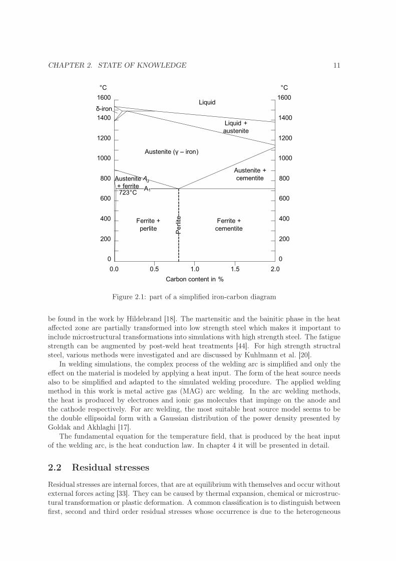
The iron-carbon phase diagram depicts the phase compositions of steel at different temper-atures depending on the carbon content. The diagram is fundamental for understanding thephase transformations of iron-carbon alloys during heating and cooling. Fig. 2.1 illustratesthe relevant part for structural steel of the simplified iron carbon diagram. The microstruc-ture of the heat affected zone (HAZ) of welded plates made of S355 was analysed by Wichers[47]. The feritic-perlitic microstructure of the base metal is transformed to austenite for tem-peratures above the upper transformation point A3. Between the lower A1 and the uppertransformation point the structure is partially austenitic. This transformation results in acoarser microstructure which leads to diminished toughness properties in the HAZ. This iswhy alterations in the mechanical behavior have an impact on the fatigue life of a structure.Therefore it is also important to analyse the temperature field and not only the residual stressfield.
For high strength structural steel like the steel type S690, little research concerning weldingsimulation has been published so far. Hildebrand [18] states that it is very important toinclude microstructural transformations in the welding simulation with high strength steel.In his work, the material properties are modeled as a compound of different microstructuresthat react individually under temperature changes. The initial microstructure of S690QLis composed of bainite and martensite which is completely transformed into austenite attemperatures above the Ac3-temperature. The microstructural transformations depend ontemperature as well as on time. Thus, the finally formed phases can be predicted by theuse of a Time-Temperature-Transformation diagram (TTT). A TTT diagram for S690 can
10
CHAPTER 2. STATE OF KNOWLEDGE 11
0
200
400
600
800
1000
1200
1400
1600
0
200
400
600
800
1000
1200
1400
1600
°C °C
0.5 1.0 1.5 2.00.0
Carbon content in %
Pe
rlite
A3
A1723°C
Ferrite +
perlite
Ferrite +
cementite
Austenite + ferrite
Austenite (γ – iron)
Liquid
Liquid +
austenite
δ-iron
Austenite +
cementite
Figure 2.1: part of a simplified iron-carbon diagram
be found in the work by Hildebrand [18]. The martensitic and the bainitic phase in the heataffected zone are partially transformed into low strength steel which makes it important toinclude microstructural transformations into simulations with high strength steel. The fatiguestrength can be augmented by post-weld heat treatments [44]. For high strength structralsteel, various methods were investigated and are discussed by Kuhlmann et al. [20].
In welding simulations, the complex process of the welding arc is simplified and only theeffect on the material is modeled by applying a heat input. The form of the heat source needsalso to be simplified and adapted to the simulated welding procedure. The applied weldingmethod in this work is metal active gas (MAG) arc welding. In the arc welding methods,the heat is produced by electrones and ionic gas molecules that impinge on the anode andthe cathode respectively. For arc welding, the most suitable heat source model seems to bethe double ellipsoidal form with a Gaussian distribution of the power density presented byGoldak and Akhlaghi [17].
The fundamental equation for the temperature field, that is produced by the heat inputof the welding arc, is the heat conduction law. In chapter 4 it will be presented in detail.
2.2 Residual stresses
Residual stresses are internal forces, that are at equilibrium with themselves and occur withoutexternal forces acting [33]. They can be caused by thermal expansion, chemical or microstruc-tural transformation or plastic deformation. A common classification is to distinguish betweenfirst, second and third order residual stresses whose occurrence is due to the heterogeneous

CHAPTER 2. STATE OF KNOWLEDGE 12
structure of materials. First order residual stresses (σI) are also called macroscopic residualstresses, because they are averaged over several crystallites. Second order residual stresses(σII) act on a smaller area, approximately between 0.01 - 1 mm. Third order residual stresses(σIII) are called microscopic residual stresses because they act between atomic areas of thesize between 10−6
− 10−2 mm. For the analysis of welding residual stress distributions, it issufficient to examine only macroscopic or first order residual stresses.
2.2.1 Welding residual stresses
The weld zone experiences high temperature differences compared to the surrounding areaduring the welding process. Under the thermal load, the material expands and is restrained bythe cooler surrounding material, which provokes stresses. Since the yield strength decreasesas the temperature increases, these stresses often exceed the yield limit and provoke plasticstrains. When plasticity occurs, existing residual stresses are relieved. This is the reason why,the initial residual stresses near the weld zone do not have any influence on the final residualstresses. On the contrary, the initial residual stresses in the parts located further away areusually not affected by welding.
The distribution of welding residual stress is very complex as it depends on several factors:
• structural dimensions
• material properties
• heat input
• number of weld passes
• welding sequence
• restraint conditions
Hence, it is difficult to predict the distribution of residual stress due to the welding op-eration. In this work, the influence of the mechanical material properties and the number ofweld passes on the resulting residual stresses are studied.
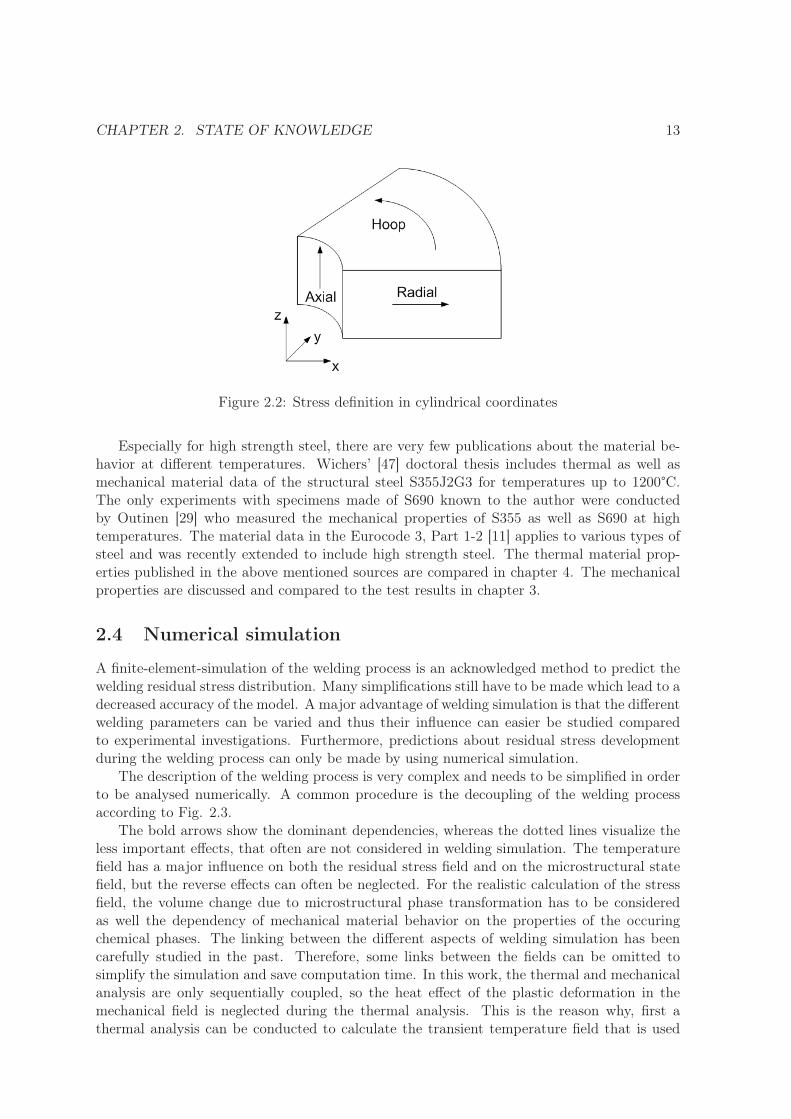
For butt-welded tubes, a cylindrical coordinate system is applied to distinguish betweenradial, hoop and axial stresses, compare Fig. 2.2. During the cooling process, the weld zoneand its vicinities shrink, hence the tube’s diameter in this zone becomes smaller and a bendingmoment is generated. This generally leads to tensile stress on the weld toe and compressiveaxial stress on the outside surface. The stress components in thickness direction are verysmall and therefore not studied in this work.
2.3 Material properties
For a realistic welding simulation it is important to properly describe the temperature de-pendent material behavior. In this work, a bilinear elastic-plastic material model was chosenand therefore the Young’s modulus and the yield strength as functions of the temperatureare required to define the stress-strain curves. Richter [37] conducted tests for different steeltypes, but only for temperatures below 600°C. Furthermore, these results can only serve toshow tendencies in the high temperature behavior. They cannot be adapted for the today’ssteel types.
CHAPTER 2. STATE OF KNOWLEDGE 13
Figure 2.2: Stress definition in cylindrical coordinates
Especially for high strength steel, there are very few publications about the material be-havior at different temperatures. Wichers’ [47] doctoral thesis includes thermal as well asmechanical material data of the structural steel S355J2G3 for temperatures up to 1200°C.The only experiments with specimens made of S690 known to the author were conductedby Outinen [29] who measured the mechanical properties of S355 as well as S690 at hightemperatures. The material data in the Eurocode 3, Part 1-2 [11] applies to various types ofsteel and was recently extended to include high strength steel. The thermal material prop-erties published in the above mentioned sources are compared in chapter 4. The mechanicalproperties are discussed and compared to the test results in chapter 3.
2.4 Numerical simulation
A finite-element-simulation of the welding process is an acknowledged method to predict thewelding residual stress distribution. Many simplifications still have to be made which lead to adecreased accuracy of the model. A major advantage of welding simulation is that the differentwelding parameters can be varied and thus their influence can easier be studied comparedto experimental investigations. Furthermore, predictions about residual stress developmentduring the welding process can only be made by using numerical simulation.
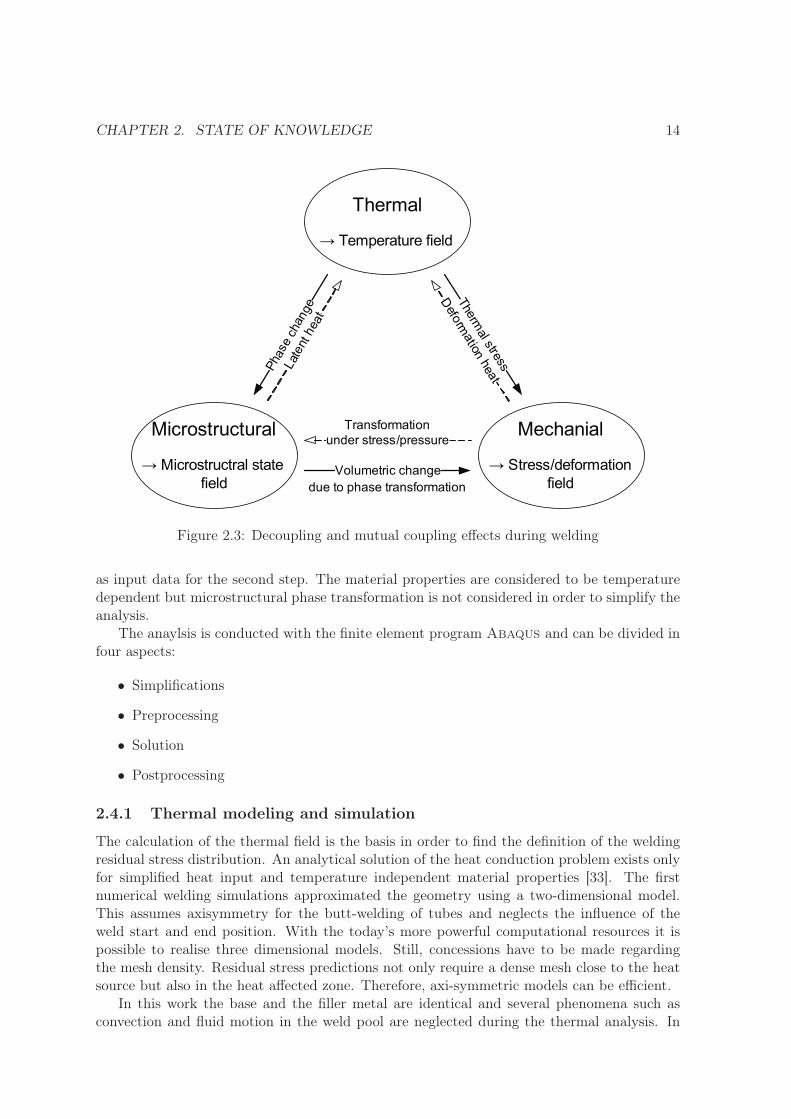
The description of the welding process is very complex and needs to be simplified in orderto be analysed numerically. A common procedure is the decoupling of the welding processaccording to Fig. 2.3.
The bold arrows show the dominant dependencies, whereas the dotted lines visualize theless important effects, that often are not considered in welding simulation. The temperaturefield has a major influence on both the residual stress field and on the microstructural statefield, but the reverse effects can often be neglected. For the realistic calculation of the stressfield, the volume change due to microstructural phase transformation has to be consideredas well the dependency of mechanical material behavior on the properties of the occuringchemical phases. The linking between the different aspects of welding simulation has beencarefully studied in the past. Therefore, some links between the fields can be omitted tosimplify the simulation and save computation time. In this work, the thermal and mechanicalanalysis are only sequentially coupled, so the heat effect of the plastic deformation in themechanical field is neglected during the thermal analysis. This is the reason why, first athermal analysis can be conducted to calculate the transient temperature field that is used
CHAPTER 2. STATE OF KNOWLEDGE 14
Thermal
→ Temperature field
Microstructural
→ Microstructral state
field
Mechanial
→ Stress/deformation
field
Phase change
Thermal stress
under stress/pressure
Latent heat
Deformation heat
Volumetric change
due to phase transformation
Transformation
Figure 2.3: Decoupling and mutual coupling effects during welding
as input data for the second step. The material properties are considered to be temperaturedependent but microstructural phase transformation is not considered in order to simplify theanalysis.
The anaylsis is conducted with the finite element program Abaqus and can be divided infour aspects:
• Simplifications
• Preprocessing
• Solution
• Postprocessing
2.4.1 Thermal modeling and simulation
The calculation of the thermal field is the basis in order to find the definition of the weldingresidual stress distribution. An analytical solution of the heat conduction problem exists onlyfor simplified heat input and temperature independent material properties [33]. The firstnumerical welding simulations approximated the geometry using a two-dimensional model.This assumes axisymmetry for the butt-welding of tubes and neglects the influence of theweld start and end position. With the today’s more powerful computational resources it ispossible to realise three dimensional models. Still, concessions have to be made regardingthe mesh density. Residual stress predictions not only require a dense mesh close to the heatsource but also in the heat affected zone. Therefore, axi-symmetric models can be efficient.
In this work the base and the filler metal are identical and several phenomena such asconvection and fluid motion in the weld pool are neglected during the thermal analysis. In
CHAPTER 2. STATE OF KNOWLEDGE 15
the single-pass models, the weld geometry is determined by the isothermal curves that exceedthe melting temperature of the material and thus the weld is not directly modeled.
For the multi-pass models, the model change option in Abaqus is used to simulate thedeposition of the filler material. Lindgren [23] called this approach, the quiet element tech-nique. With the model change option, the elements of the next weld pass are activated all atonce after the completion of the previous weld pass. To activate the elements means to assignthem realistic material properties. Deactivated elements are not actually removed from themodel, but assigned zero valued material properties. In the heat flow model, the conductiv-ity is therefore set to zero whereas in the mechanical analysis the stiffness is assumed to bezero. When activating the elements for the models in this work, they are added as strain freeelements. The technique, that does not activate the elements of an entire weld pass, but thatactivates the elements when the filler material is actually deposited, is the so called elementbirth technique. This approach is more realistic, but it also complicates the analysis and ismore time consuming.
2.4.2 Simulation programs
In this work, the finite element program Abaqus was used to simulate the welding procedureand calculate the residual stress field. Abaqus/cae provides a coherent graphical interface,that is very helpful to create the geometry and the mesh. For more specific changes on themodel, an input file can be created and afterwards modified. The heat input is modeledby the user subroutine Dflux that is written as Fortran code. Temperature dependentmaterial behavior can be realised without programming a user subroutine and a user-specifiedmaterial model can be implemented with the subroutine Umath. It is possible to model thewelding analysis with Abaqus as a coupled thermal-stress analysis. Abaqus also provides aninterface to model two-dimensional welding simulations that faciliates the setup of the model.
Another software that is used in many other works to model a welding procedure isAnsys. A major advantage compared to Abaqus is the Ansys element birth and deathprocedure to simulate the filler material deposition. Volz [46] developed a macro to simulatethe temperature dependent material behavior of structural steel. Together with other researchinstitutions, Cadfem designed the welding simulation tool Sst that can be used in combina-tion with Ansys to faciliate the modeling of the complicated processes during welding suchas microstructural transformations and the heat source.
Furthermore, welding can be simulated with the software Sysweld, that is also basedon the finite element method. The analysis is divided into a thermo-microstructural and amechanical part. Sysweld allows a more realistic simulation of the material behavior bymodelling it as a composition of different microstructures. Therefore, transformation effectsas strains and plasticity can be taken into consideration. The downside of this software isthat a large number of material data are needed. To avoid the costly and time consumingdetermination of these data sets, values are often extrapolated which decreases the accuracyof the material model and therefore the advantage of Sysweld . Secondly, high computationtimes are required that restrict the density of the mesh [42]. The geometry and the mesh caneither be generated with Sysweld or be imported.

Chapter 3
Experiments
In numerical welding simulations not only input data of the geometry, the heat source, and theboundary conditions must be known but also the temperature dependent material behavior.In order to model the welding process as realistically as possible, it is fundamental to useaccurate values for the thermal and mechanical material model. The experiments in thiswork aimed to verify the temperature dependent reduction factors for the yield stress andthe Young’s modulus given in the Eurocode 3 [11]. The yield stress and Young’s modulusare used to define an ideal elastic-plastic material model and they can be deduced from thestress-strain curve. In order to find the deformational behavior and hence the stress-straincurves, a tensile testing is conducted. Therefore, specimens made of two different structuralsteels, S355 and S690, were tested at three different temperatures in a tensile test.
3.1 Specimen geometry
To faciliate the comparability to earlier test results, the following relation is used to definethe proportion between the initial gage length L0 and the initial cross section S0:
L0 = k ·
√
S0 (3.1)
The international default value for k is 5.65, which results from the conversion of a round spec-imen to a rectangular form. For round specimens with the initial diameter d0, the simplifiedrelation 3.2 can be used [14].
L0 = 5 · d0 (3.2)
The tests in this work where conducted with round specimens made of two different structuralsteels, S355 and S690, with the geometry shown in Fig. 3.1. A round form was chosen inorder to obtain a uniform temperature distribution. The aim was also to use the smallestdiameter as possible so that the specimen heats up fast to save energy. Even though thecode proposes also smaller specimen it is also noted that it is not advised to experiment withsmaller specimen because it requires greater skill in testing.
The gage section has to be the smallest section, to provoke the failure to occur in thisarea. The outer part of the specimen is the so called shoulder, where the specimen is grippedby the machine. The specimens were taken out of the tubes that were used for the numericalmodels in chapter 5.
16

CHAPTER 3. EXPERIMENTS 17
Figure 3.1: Specimen geometry according to the ASTM E8M-09 [40]
3.2 Performance of the tests
The tests were conducted at three different temperatures, namely room temperature, 250°Cand 800°C. The temperatures 250°C and 800°C were chosen according to the above mentionedthesis by Wichers [47]. Using his results for specimens made of S355J2G3 to trace the Young’smodulus as a function of temperature, one can observe a transition of behavior at the abovementioned temperatures. Furthermore, choosing 800°C as the highest testing temperatureseems to be sufficient. It was stated in the doctoral thesis by Barsoum [2] on residual stressanalysis for welded steel structures that this temperature is used as a cut-off-temperaturein the finite element model, because the yield limit is disappearing in the high temperaturerange, so that no residual stresses are developed. Therefore the material properties in thehigh temperature range are assumed to be the same as at a fixed cut-off temperature. Ingeneral, the cut-off temperature is chosen to be half of the melting temperature:
Tcut−off = 0.5 · Tmelt (∼= 700◦C) (3.3)
It was chosen to conduct the tests at 800°C instead of 700°C because at around 700°C a phasetransformation takes place, that was not desired for the study to be captured.
The deformational behavior of steel at elevated temperatures is dependent on the defor-mation rate. The American code for elevated temperature tensile tests, the ASTM E21-09[39], indicates a strain rate of 0.005 min−1. The corresponding European code EN 10002-5[14] suggests a strain rate in the range of 0.001 and 0.005 min−1 for the yield stress deter-mination. After having exited the elastic zone the strain rate can be augmented. In orderto use values, that are realistic for a welding procedure, the strain rates were derived froma cooling curve after welding. Therefore, a significant point within the weld in a model of awelded tubular K-joint was chosen and the temperature development during cooling analyzed[1]. The strain rate was then calculated by multiplying the thermal expansion factor α withthe first derivative with respect to the time:
v = αdT
dt(3.4)
The values for the thermal expansion coefficient were taken from Wichers [47]. Becauseof the big impact of the strain rate on the test results, it was chosen to raise the strain rateduring the experiments on the one hand to capture the effect on the stress-strain curve and,on the other hand, to save energy.

CHAPTER 3. EXPERIMENTS 18
In order to minimize the influence of scatter due to the material properties or geometricdefaults, for each temperature either two or three tests were chosen to be conducted with thesame strain rate. For the tests at room temperature the strain rates were chosen accordingto the codes, because the deformational behavior is not strain rate dependent. It was decidedto only conduct two tests at room temperature, because there are many other test resultsavailable. By using the relation 3.4 a strain rate of 0.002 min−1 was calculated for the testsat 250°C. Since this strain rate is within the range that the European code indicates, it waschosen to conduct three tests with this strain rate and to augment the strain rate by a factorof ten after the elastic zone has been captured. For the tests at 800°C, the cooling occursfaster than for the lower temperatures which is why a faster strain rate of 0.05 min−1 wascalculated. As this is out of the range of the strain rates given by the codes, it was decided toconduct four tests at 800°C, whereof two tests use the strain rate of the code for the elasticzone and a strain rate ten times faster for the plastic zone. The second pair of tests uses thefaster strain rate during the entire tests. As a conclusion, the four stress-strain curves shouldmatch in the plastic zone, where they were all conducted with the same strain rate.
Figure 3.2: Test set-up
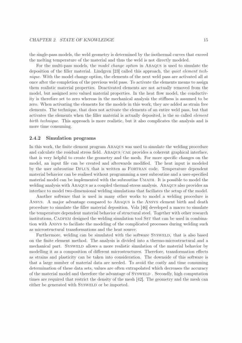
The tensile tests were conducted on a machine produced by Mohr & Federhaff AG (MFL)(Fig. 3.2). Before the specimen was installed into the machine, all the grips had to be carefullygreased with a high temperature resistant grease. After the placement of the specimen,the thermocouple was inserted into a nut around the specimen (Fig. 3.3, to measure thetemperature during the test. This temperature measurement set-up, was calibrated prior tothe tests using a drilled specimen to compare the temperatures within the gage length to thetemperature measured in the nut. With a stabilisation time of 5 minutes before the test it wasassured, that the temperature would vary no more than 3°C within the gauge length duringthe test.
The deformation was evaluated with an extensometer (Fig. 3.3) that measured the rotationof two arms that were placed on the specimen. The initial distance between the two armswere 15 mm. After the oven was closed and insulated, the specimen was heated by radiation,which can result in a very fast heating process. Therefore, it had to be taken care that thetemperature did not overshoot for the tests at 250°C. During the heating process, the machinehad to work on load control. Otherwise, the specimen would have been under compressionand possibly have buckled. After the temperature distribution was stable, the test was startedon deformation control. It was not possible to control the test and measure the deformation
CHAPTER 3. EXPERIMENTS 19
Figure 3.3: Specimen with thermocouple and extensometer
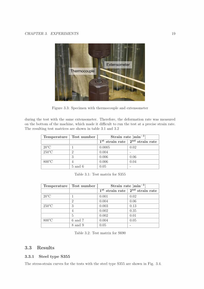
during the test with the same extensometer. Therefore, the deformation rate was measuredon the bottom of the machine, which made it difficult to run the test at a precise strain rate.The resulting test matrices are shown in table 3.1 and 3.2
Temperature Test number Strain rate [min−1]
1st strain rate 2nd strain rate
20°C 1 0.0005 0.02250°C 2 0.004 -
3 0.006 0.06800°C 4 0.006 0.04
5 and 6 0.05 -
Table 3.1: Test matrix for S355
Temperature Test number Strain rate [min−1]
1st strain rate 2nd strain rate
20°C 1 0.001 0.022 0.004 0.06
250°C 3 0.003 0.134 0.002 0.355 0.002 0.01
800°C 6 and 7 0.004 0.058 and 9 0.05 -
Table 3.2: Test matrix for S690
3.3 Results
3.3.1 Steel type S355
The stress-strain curves for the tests with the steel type S355 are shown in Fig. 3.4.

CHAPTER 3. EXPERIMENTS 20
0 1 2 3 4 5 6 7 8 9 100
100
200
300
400
500
600
Strain [%]
Str
ess
[M
Pa
]
20°C
250°C
800°C
Figure 3.4: Stress-Strain curves of tests with S355
Test 2 at 250°C ended before the strain rate could have been augmented, because theextensometer slipped on the specimen. However, the test was sufficiently long to capture theyield stress. For the tests at 800°C, two different strain rates were used in principle. Forthe test 4, the elastic zone was captured by using approximately the strain rate given by theASTM E21-09 [39]. At about 3%-strain, the strain rate was augmented to the value calculatedwith 3.4. During tests 5 and 6 the strain rate was maintained at the same value as for thesecond part in test 4. As it can be seen, the three curves are in very good agreement in theplastic zone, where the tests were run with approximately the same strain rate.
Temperature Test number Young’s modulus [GPa] RP0.2 [MPa] RP2.0 [MPa]
20°C 1 205.2 428.9250°C 2 171.3 378.4 -
3 182.2 381.5 476.6800°C 4 41.3 47.7 52.9
5 33.8 60.27 69.76 44.8 58.73 69.9
Table 3.3: Summary of the results for the tests with S355
The Young’s modulus was evaluated as tangent modulus in the elastic zone. The yieldstrength was determined at an offset of 0.2 % as described in the ASTM E21-09 [39]. For theelevated temperatures it was also evaluated at an offset of 2 %. The obtained values for theYoung’s modulus and the yield stress are listed in Table 3.3.
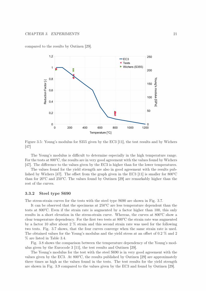
The values obtained by the tests were compared to the reduction factors given by theEurocode 3 for fire design of steel structures [11] as well as the values found by Wichers [47].Fig. 3.5 shows this comparison for the Young’s modulus. In Fig. 3.6, the reduction factors forthe yield strength were calculated with the values at an offset of 0.2 % strain and additionally
CHAPTER 3. EXPERIMENTS 21
compared to the results by Outinen [29].
Figure 3.5: Young’s modulus for S355 given by the EC3 [11], the test results and by Wichers[47]
The Young’s modulus is difficult to determine especially in the high temperature range.For the tests at 800°C, the results are in very good agreement with the values found by Wichers[47]. The difference to the values given by the EC3 is higher than for the lower temperatures.
The values found for the yield strength are also in good agreement with the results pub-lished by Wichers [47]. The offset from the graph given in the EC3 [11] is smaller for 800°Cthan for 20°C and 250°C. The values found by Outinen [29] are remarkably higher than therest of the curves.
3.3.2 Steel type S690
The stress-strain curves for the tests with the steel type S690 are shown in Fig. 3.7.It can be observed that the specimens at 250°C are less temperature dependent than the
tests at 800°C. Even if the strain rate is augmented by a factor higher than 100, this onlyresults in a short elevation in the stress-strain curve. Whereas, the curves at 800°C show aclear temperature dependency. For the first two tests at 800°C the strain rate was augmentedby a factor 10 after about 2 % strain and this second strain rate was used for the followingtwo tests. Fig. 3.7 shows, that the four curves converge when the same strain rate is used.The obtained values for the Young’s modulus and the yield stress at an offset of 0.2 % and 2% are listed in Table 3.4.
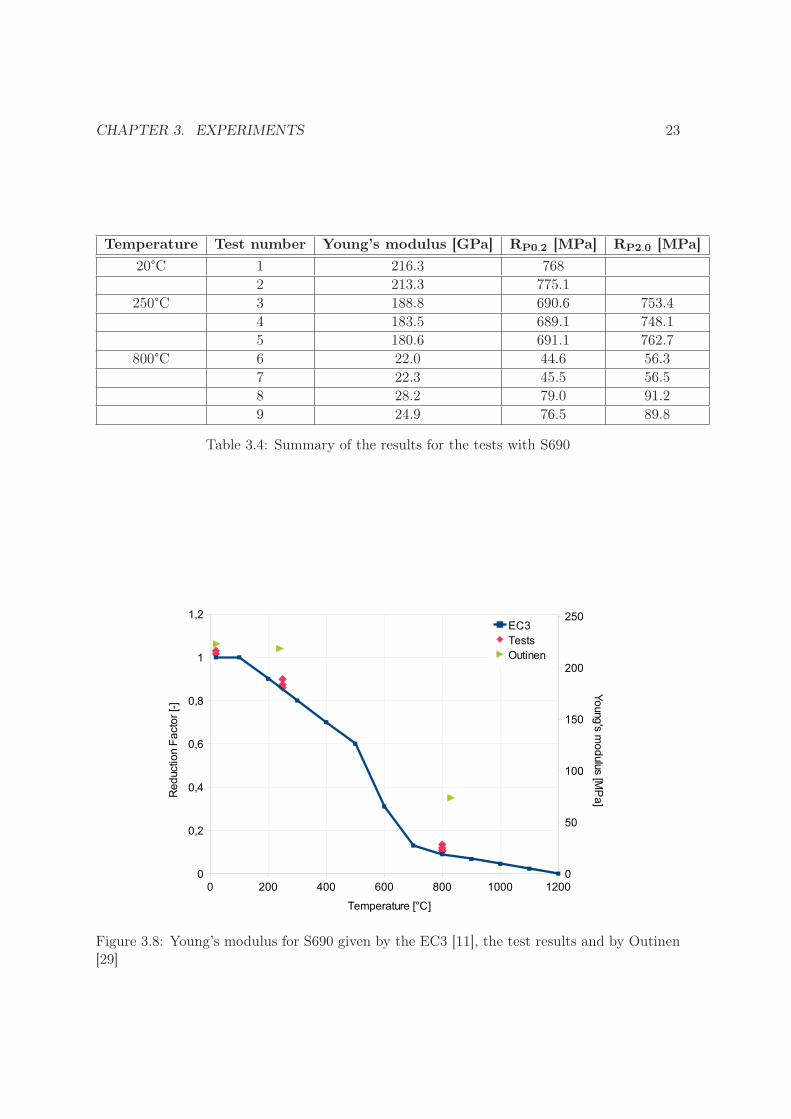
Fig. 3.8 shows the comparison between the temperature dependency of the Young’s mod-ulus given by the Eurocode 3 [11], the test results and Outinen [29].
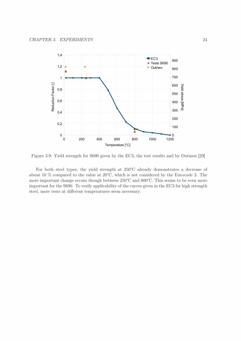
The Young’s modulus for the test with the steel S690 is in very good agreement with thevalues given by the EC3. At 800°C, the results published by Outinen [29] are approximatelythree times as high as the values found in the tests. The test results for the yield strengthare shown in Fig. 3.9 compared to the values given by the EC3 and found by Outinen [29].

CHAPTER 3. EXPERIMENTS 22
Figure 3.6: Yield strength for S355 given by the EC3, the test results, by Wichers [47] andby Outinen [29]
0 1 2 3 4 5 6 7 80
100
200
300
400
500
600
700
800
900
Strain [%]
Str
ess
[M
Pa
]
20°C
250°C
800°C
Figure 3.7: Stress-Strain curves of tests with S690
CHAPTER 3. EXPERIMENTS 23
Temperature Test number Young’s modulus [GPa] RP0.2 [MPa] RP2.0 [MPa]
20°C 1 216.3 7682 213.3 775.1
250°C 3 188.8 690.6 753.44 183.5 689.1 748.15 180.6 691.1 762.7
800°C 6 22.0 44.6 56.37 22.3 45.5 56.58 28.2 79.0 91.29 24.9 76.5 89.8
Table 3.4: Summary of the results for the tests with S690
Figure 3.8: Young’s modulus for S690 given by the EC3 [11], the test results and by Outinen[29]
CHAPTER 3. EXPERIMENTS 24
Figure 3.9: Yield strength for S690 given by the EC3, the test results and by Outinen [29]
For both steel types, the yield strength at 250°C already demonstrates a decrease ofabout 10 % compared to the value at 20°C, which is not considered by the Eurocode 3. Themore important change occurs though between 250°C and 800°C. This seems to be even moreimportant for the S690. To verify applicability of the curves given in the EC3 for high strengthsteel, more tests at different temperatures seem necessary.
Chapter 4
Numerical simulation
4.1 Thermal analysis
4.1.1 Theory
The fundamental principles for the field equation of heat conduction are the Conservation ofEnergy and the Fourier’s law. By definition temperature is a time dependent scalar field:
T = T (x, y, z, t) (4.1)
The conjugate thermodynamic quantity is the heat flux density q, which defines the heat fluxper area.
q = [qx, qy, qz]T (4.2)
Fouriers law of heat conduction states that the heat flow q is proportional to the negativetemperature gradient generated by a temperature difference (heat flows from high to lowtemperature zones). With the assumption that steel is a homogenous and isotropic materialthis can be written as follows:
q = −λ grad (T ) (4.3)
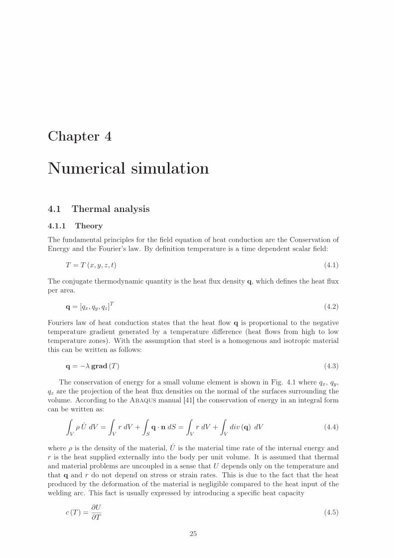
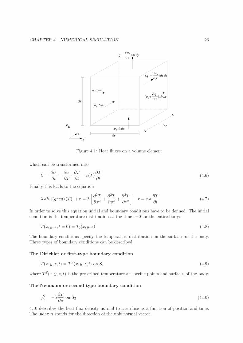
The conservation of energy for a small volume element is shown in Fig. 4.1 where qx, qy,qz are the projection of the heat flux densities on the normal of the surfaces surrounding thevolume. According to the Abaqus manual [41] the conservation of energy in an integral formcan be written as:
∫
Vρ U dV =
∫
Vr dV +
∫
Sq · n dS =
∫
Vr dV +
∫
Vdiv (q) dV (4.4)
where ρ is the density of the material, U is the material time rate of the internal energy andr is the heat supplied externally into the body per unit volume. It is assumed that thermaland material problems are uncoupled in a sense that U depends only on the temperature andthat q and r do not depend on stress or strain rates. This is due to the fact that the heatproduced by the deformation of the material is negligible compared to the heat input of thewelding arc. This fact is usually expressed by introducing a specific heat capacity
c (T ) =∂U
∂T(4.5)
25
CHAPTER 4. NUMERICAL SIMULATION 26
Figure 4.1: Heat fluxes on a volume element
which can be transformed into
U =∂U
∂t=
∂U
∂T·
∂T
∂t= c(T )
∂T
∂t(4.6)
Finally this leads to the equation
λ div [(grad) (T )] + r = λ
[
∂2T
∂x2+
∂2T
∂y2+
∂2T
∂z2
]
+ r = c ρ∂T
∂t(4.7)
In order to solve this equation initial and boundary conditions have to be defined. The initialcondition is the temperature distribution at the time t=0 for the entire body:
T (x, y, z, t = 0) = T0(x, y, z) (4.8)
The boundary conditions specify the temperature distribution on the surfaces of the body.Three types of boundary conditions can be described.
The Dirichlet or first-type boundary condition
T (x, y, z, t) = TS(x, y, z, t) on S1 (4.9)
where TS(x, y, z, t) is the prescribed temperature at specific points and surfaces of the body.
The Neumann or second-type boundary condition
qSn = −λ∂T
∂non S2 (4.10)
4.10 describes the heat flux density normal to a surface as a function of position and time.The index n stands for the direction of the unit normal vector.

CHAPTER 4. NUMERICAL SIMULATION 27
The Robin or third-type boundary condition The Robin boundary conditions de-scribes the heat transfer to the surrounding medium by
qSn = h (T − T0) on S3 (4.11)
where h is the heat transfer coefficient and T0 is the gas or liquid temperature of the surround-ing medium. In this boundary condition, the heat transfer is proportional to the temperaturedifference between the surface and the ambiance and includes convection and radiation. Theheat transfer coefficient h can be temperature dependent.
Heat transfer by convection Heat transfer by convection occurs in liquids or gases causedby movement of molecules. It can be distinguished between natural and forced convection.Natural convection can only occur in a gravity field because the movement is due to thedifferences in density caused by temperature gradients. Forced convection is the result whenexternal forces maintain the movement (e.g. a fan or the blow effect of the welding arc). TheNewton’s law describes convection with
qc = hc (T − T0) (4.12)
where hc is the heat transfer coefficient due to convection. The heat transfer coefficientis dependent on the flow conditions, the surface and temperature differences between thematerial and the surroundings.
Heat transfer by radiation According to the Stephan-Boltzmann’s law the heat flow den-sity of a gray body caused by radiation is proportional to the forth power of the temperaturedifferences to its surroundings:
qr = ǫσ0(
T 4− T 4
0
)
(4.13)
where ǫ is the emissivity and σ0 is the Stefan-Boltzmann constant (= 5.670 · 10−8W/m2K4).The emissivity can be temperature dependent in the high temperature range. By linearizingequation 4.13 the heat flow density caused by radiation can be expressed in the same form asthe heat flow density due to convection, so that both boundary conditions can be combined.
4.1.2 Finite Element solution
The analytical solution of equation 4.7 can only be obtained for simple geometries, boundaryconditions and temperature independent material properties. That is why the use of a finiteelement procedure can be necessary. We start with what is called the Galerkin formulation bymultiplying equation 4.7 with a virtual weighting function δT and integrating over the entirevolume:
∫
S
δT λgrad (T ) ·ndS−
∫
V
grad (T ) ·λ ·grad (δT ) dV +
∫
V
r δT dV =
∫
V
cρ∂T
∂tdV (4.14)
Introducing the boundary conditions into equation 4.14 and using the Gauss theorem we get:∫
V
grad (δT ) · λ grad (T ) dV +
∫
V
δTρc∂T
∂tdV =
∫
V
δT r dV +
∫
S
δT q dS (4.15)
CHAPTER 4. NUMERICAL SIMULATION 28
where the Qi are concentrated heat flow inputs. The principle of virtual temperatures isused in the same way as the more common principle of virtual displacements, that is, inorder to determine the unknown temperature field at its nodes. One major difference here incomparison to elastostatics is the presence of the time variable, which in general is treatedseparately. So the next step is to define the temperature field by separating the time andspace dependency:
T = T (x, y, z, t) = N (x, y, z) ·T (t) (4.16)
The same can be done for the virtual temperature field δT. Here already the next stepis included, which is to discretize the body and assume it to be a batch of so called finiteelements. So the vector T (t) contains the temperature evolution at the nodes of the finiteelements. In the matrix N the so called shape or interpolation functions are stored. Thenext step would be now to define properly the shape functions Ne at an element level, whichwill be omitted here (for the case of continuum elements it is referred here to the Abaqusmanual [41]). If the preceding formulations are inserted into 4.15 and the virtual energy isassembled over the whole body, the principle finite element equations in heat transfer analysisare obtained:
CT+(
Kλ +Kconv +Krad)
T = Qinp +Qconv +Qrad (4.17)
where C is the heat capacity matrix,
C =∑
e
∫
Ve
NTe ρcNe dV (4.18)
Kλ is the conductivity matrix,
Kλ =∑
e
∫
Ve
BTe λBe dV (4.19)
Kconv is the convection matrix,
Kconv =∑
e
∫
Sconv
hconv NTe Ne dS (4.20)
and Krad is the radiation matrix
Krad =∑
e
∫
Srad
hrad NTe NedS (4.21)
The vector of the heat flow input Qinp is given by:
Qinp = QB + QS (4.22)
where QB is a volumetric heat flow input
QB =∑
e
∫
Ve
NTe r dV (4.23)

CHAPTER 4. NUMERICAL SIMULATION 29
and QS is a surface heat flow input
QS =∑
e
∫
Se
NT qSdS (4.24)
The heat flows Qconv and Qrad in equation 4.17 are due to convection and radiationboundary conditions. For the temperature distribution of the surrounding medium the sameinterpolations as for the surface temperatures are used and for the radiation boundary condi-tion the linearized form is used, which leads to:
Qconv =∑
e
∫
Sconv
hconv NTe ·Ne ·T0 dS (4.25)
Qrad =∑
e
∫
Srad
hrad NTe ·Ne ·T0 dS (4.26)
By combining the conductivity, the convection, and the radiation matrix as well as the heatsupply vectors 4.17 can be written as
C T+KT = Q (4.27)
In order to numerically solve the semidiscrete heat equation, the time interval for the solutionhas to be divided into different increments. The equation system is therefore only evaluatedat every discrete time n ·∆t. The most common algorithms to solve a parabolic problem asthe heat transfer are the generalized trapezoidal methods.
4.1.3 Heat source
The complex process in the weld pool is simplified by neglecting material movement in themolten zone including heat transfer by convection and radiation. Therefore, the heat sourcemodel only describes the effect of the heat source. The principle parameter used in the heatsource model is the heat quantity Q [J] in momentarily acting sources. The heat losses duringthe complex processes of welding are considered by the heat efficiency ηh and combine thelosses by radiation of the weld arc, heat dissipation by convection and spray losses. The heatflow q [J/s] for continuously acting sources is the product of voltage U [V], amperage I [A]and heat efficiency:
q = η UI (4.28)
The heat efficiency for gas metal arc welding is estimated in the range of 0.65 and 0.90.Another parameter, that has an important influence on the temperature field, is the weldingspeed that for gas metal arc welding usually lies below 15 mm/s [33]. The spatial distributionof the welding source can either be a point, a surface or a volume source. In general, surfaceand volume sources are preferred for the finite element model because they seem to be morerealistic. Also, a surface and a volume source can be combined [21], where the surface heatinput models the heat by the welding arc and the volumetric heat source simulates the heatinput of the melt drops.
The most common heat source models use Gaussian normal distributions over a circularsurface or a hemisphere (figure 4.2). Another approach to simulate the welding source isby prescribing temperatures as boundary conditions. For the models in this work either ahemispherical or a spherical volumetric heat source with uniform heat flux density is used.

CHAPTER 4. NUMERICAL SIMULATION 30
Figure 4.2: Welding heat sources with Gaussian distribution of the surface heat flux densityqsurf and the volume heat flux density qvol [35]
4.1.4 Thermal material properties
For the heat transfer analysis, temperature dependent curves for the thermal conductivity λ,the specific heat capacity c and the density ρ are needed. Richter [37] conducted many teststo obtain these material characteristics for different steel types, but only for temperatures upto 600°C. For the structural steel grade S355, values at high temperatures can be found ina work by Wichers [47]. There are no tests for structural high strength steel as S690 knownto the author. The Eurocode 3 [11] provides temperature dependent values for the thermalconductivity and the specific heat capacity but without distinguishing between different steeltypes. The same material properties were used for the filler and the base metal.
Figure 4.3: Thermal conductivity λ according to EC3 and Wichers [47]
Thermal conductivity Fig. 4.3 presents the thermal conductivity given in the Eurocodecompared to the values found by Wichers [47]. For the Abaqus models in this work the data

CHAPTER 4. NUMERICAL SIMULATION 31
from the EC 3 is used. For temperatures above the melting temperature, the conductivityis multiplied by three to account for heat transfer by convection in the weld pool. Wichers[47] calculated the thermal conductivity from the values obtained for the electric resistanceby using the Wiedemann Franz law.
Specific heat capacity During phase transformations, the material loses or accumulatesenergy without changing its temperature. To capture this so called latent heat in a numericalsimulation, either the specific heat can show a significant maximum at phase transformationtemperatures or a latent heat has to be considered. Therefore, the Eurocode uses a significantmaximum for the α-γ-transformation at 735°C. To account for the solid-liquid phase change,a latent heat of 247000 J/kg is used in the Abaqus models in this work refering to Raymondand Chipman [36]. Fig. 4.4 shows that Wichers [47] considered a lower maximum for thespecific heat than the Eurocode.
Figure 4.4: Specific heat c according to EC3 and Wichers [47]
Density The density can be calculated by using the relation with the coefficient of thermalexpansion, that is given in Chapter 4.2.2. This is the reason why, Wichers [47] finds adiscontinuity point at the temperature where phase transformation occurs. The Eurocodespecifies a constant density. Richter [37] proposes to use a linear approach for the densitybetween termperatures from 0 to 1000°C, which is in good agreement with the values foundby Wichers [47]. For the thermal analysis in the abaqus models, the constant density fromthe Eurocode was considered.
4.1.5 Boundary conditions
Convection and radiation are considered for modeling boundary heat transfer. The valueswere taken from Brown and Song [5] who assumed that the film coefficient for convective heattransfer is dependent on temperature and orientation of the boundary. By using the linearized

CHAPTER 4. NUMERICAL SIMULATION 32
Figure 4.5: Density ρ according to EC3 and Wichers [47]
form for radiation, both boundary conditions were combined:
htotal = hconv + hrad
hrad = ǫσ(
T 3 + T 2T0 + TT 20+ T 3
0
)(4.29)
where σ is the Stefan-Boltzmann constant and T0 is the reference sink temperature value. Itwas assumed that radiation occurs only from the surface to the ambient air and not betweensurfaces. So, no radiation on the inside of the tubes was considered.
At low temperatures, the heat flow by convection and radiation is small compared to theheat transfer by conduction. This is why, the thermal boundary conditions were only appliedon the outer surface of the tubes close to the weld in order to save computation time.
Figure 4.6: Film coefficient due to convection hconv and due to radiation hrad according toBrown and Song [5]
CHAPTER 4. NUMERICAL SIMULATION 33
4.2 Mechanical analysis
4.2.1 Theory
As was mentioned above, the thermal and mechanical processes in this work were consideredto be only sequentially coupled. Therefore, the thermal analysis is followed by a mechanicalanalysis where the nodal temperature histories calculated in the thermal analysis are used asinput data to calculate the resulting strains during welding. The same finite element mesh isused as for the thermal analysis and linear brick elements with reduced integration are usedwith three degrees of freedom at each node.
The basis for classic finite elements in mechanics is the equilibrium formulation writtenas principle of virtual work:
∫
Vσσσ : δεεε dV =
∫
SδnT
· σσσ · δu dS +
∫
Vf · δu dV (4.30)
where
εεε =1
2
[
grad (u) + gradT (u)]
(4.31)
is the linearised strain tensor derived from the displacement field, defining a linear operator onthe displacement field. δu is a virtual displacement field and δε is the virtual strain derived bythe strain operator from the virtual displacement field. Until now no hypothesis was made forthe constitutive equations. The finite element solution is then implemented by interpolatingu between a finite number of points, the nodes defining the finite element mesh:
u = N ue (4.32)
For an exact description of the implementation of the specific elements reference is made tothe Abaqus manual [41].
In this work the chosen material model is an isotropic elasto-plasticity model which isoften used for metals because of its simple form. When neglecting the strain components dueto volumetric change during phase transformation, transformation plasticity and creeping,the total strain can be written as follows:
εεε = εεεel + εεεpl + εεεth (4.33)
where the components represent elastic, plastic and thermal strain respectively. The straintensor, as every tensor of second order, can be decomposed in a volumetric and a deviatoriccomponent:
εvol = trace (εεε) (4.34)
and
e = εεεdev = εεε−1
3εvolI (4.35)
This procedure is valid for each component of the strain tensor. Additionally, the stresstensor σσσ can be decomposed in the same manner:
p = −
1
3trace (σσσ) (4.36)
CHAPTER 4. NUMERICAL SIMULATION 34
and
s = σσσ + pI (4.37)
With introducing the bulk and the shear modulus, that are computed using the tempera-ture dependent Young’s modulus E (T ) and Poisson’s ratio ν (T ) given by the user as inputvalue:
K(T ) =E(T )
3 (1− 2ν(T ))(4.38)
G(T ) =E(T )
2 (1 + ν(T ))(4.39)
the elasticity law can be rewritten as follows:
p = −K(T )εvol (4.40)
and
s = 2G(T )eel (4.41)
The transition from elastic to plastic behavior, where non-reversible deformations occur,is called yield. The plasticity model in this work is assumed to be rate independent and usesthe von Mises yield criterion. The yield condition for the von Mises criterion is expressed as:
q − fy = 0 (4.42)
where
q =
√
3
2s : s (4.43)
and fy is the yield stress, that is dependent on the equivalent plastic strain epl and on thetemperature Abaqus. The flow rule assumes that yielding occurs in the direction normal tothe yielding surface defined by the von Mises criteria:
depl = epln (4.44)
where
n =3
2s
q(4.45)
Strain hardening was not considered in this work to simplify the analysis. The equations4.42 to 4.45 describe the material behavior in an incremental form. For each increment ateach point q is calculated and compared to the yield stress fy. If this value is reached, plasticflowing occurs and the incremental equations are integrated by using the Euler backwardmethod. The thermal strains are generated by the thermal expansion coefficients α shown inFig. 4.8 according to the expression:
εεεth = α(T ) (T − T0)) I (4.46)
where T0 is the reference temperature.

CHAPTER 4. NUMERICAL SIMULATION 35
4.2.2 Mechanical material properties
The mechanical material properties are considered to be temperature dependent, but thereare very few experimental data for the material behavior at high temperatures of structuralsteel. Therefore, the reduction factors from the Eurocode 3, Part 1-2 were used for the bilinearelastic-plastic material model in Abaqus. The temperature dependent values of the Young’smodulus and the yield stress given by the Eurocode 3 are shown in Fig. 4.7. The Poisson’sratio is assumed to be a constant value of 0.3.
Figure 4.7: Young’s modulus and Yield strength according to EC3
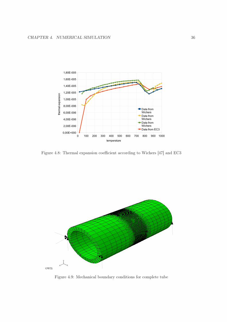
Thermal expansion factor The thermal expansion coefficient is needed to calculate thethermal dilatation due to a change of temperature. Fig. 4.8 shows the thermal expansioncoefficient measured by Wichers [47] with three different devices and the values given in theEurocode 3. It can be seen that the curve changes between 700 and 850°C. This is due to achange of microstructure and occurs for all the curves in the same temperature range. Forthe Abaqus models, the thermal expansion coefficient from the Eurocode 3 were chosen.
Especially for the multi-pass model it is important to include an annealing function duringthe mechanical analysis to simulate the relaxation of plastic stresses and strains of the remeltedmaterial. This relaxation is due to different microstructural processes as recrystallization andrapid creep [28]. For the annealing function in Abaqus, a temperature can be specified overwhich all plastic strains are set to zero. In this work, the melting temperatures is estimatedto 1465°C and is also chosen for the annealing temperature.
4.2.3 Boundary conditions
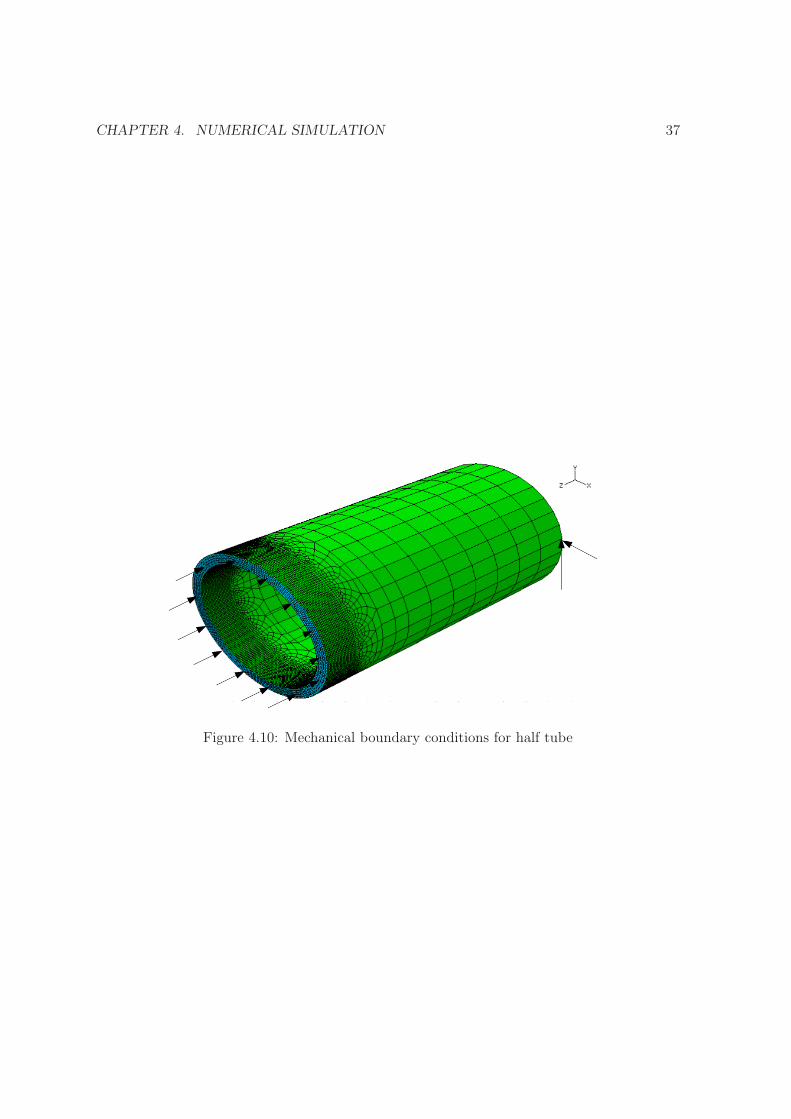
The boundary conditions in the mechanical analysis are chosen to only prevent rigid bodymovement and are applied 200 mm away from the weld centerline. Fig. 4.9 shows theboundary conditions when the entire tube is modeled and Fig. 4.10 when only half of thetube in axial direction is modeled. For the model in Fig. 4.10 all the nodes at the weld centerhave to be constrained in axial direction as symetric boundary conditions whereas the far endfrom the weld has to be free to move axially but constrained in the other directions.
CHAPTER 4. NUMERICAL SIMULATION 36
Figure 4.8: Thermal expansion coefficient according to Wichers [47] and EC3
own
Figure 4.9: Mechanical boundary conditions for complete tube
CHAPTER 4. NUMERICAL SIMULATION 37
Figure 4.10: Mechanical boundary conditions for half tube
Chapter 5
Finite Element Models
All the models in this work are developed based on the Abaqus software listed in Chapter2.4.2. Only three-dimensional and no axisymmetric models were analysed. The steel types,S355 and S690, and dimensions are chosen according to a study at the EPFL (École Polytech-nique Fédérale de Lausanne). It is assumed that the temperature field is not dependent on thestress or deplacement solution, so the analysis was conducted sequentially coupled. First thetemperature distribution is calculated in a heat transfer analysis and then applied as a loadduring the mechanical analysis. The assumption made is that only small displacements occurduring welding. The decoupling of the two analysis steps is an acknowledged simplificationto save computation time.
Besides decoupling the analysis, various assumptions and simplifications were made inorder to simulate the welding procedure in an efficient way. To verify the chosen modellingtechnique and to estimate the influence of the simplifications in this work, the model analysedin the publication by Karlsson and Josefson [19] is simulated.
5.1 Verification of the modelling technique
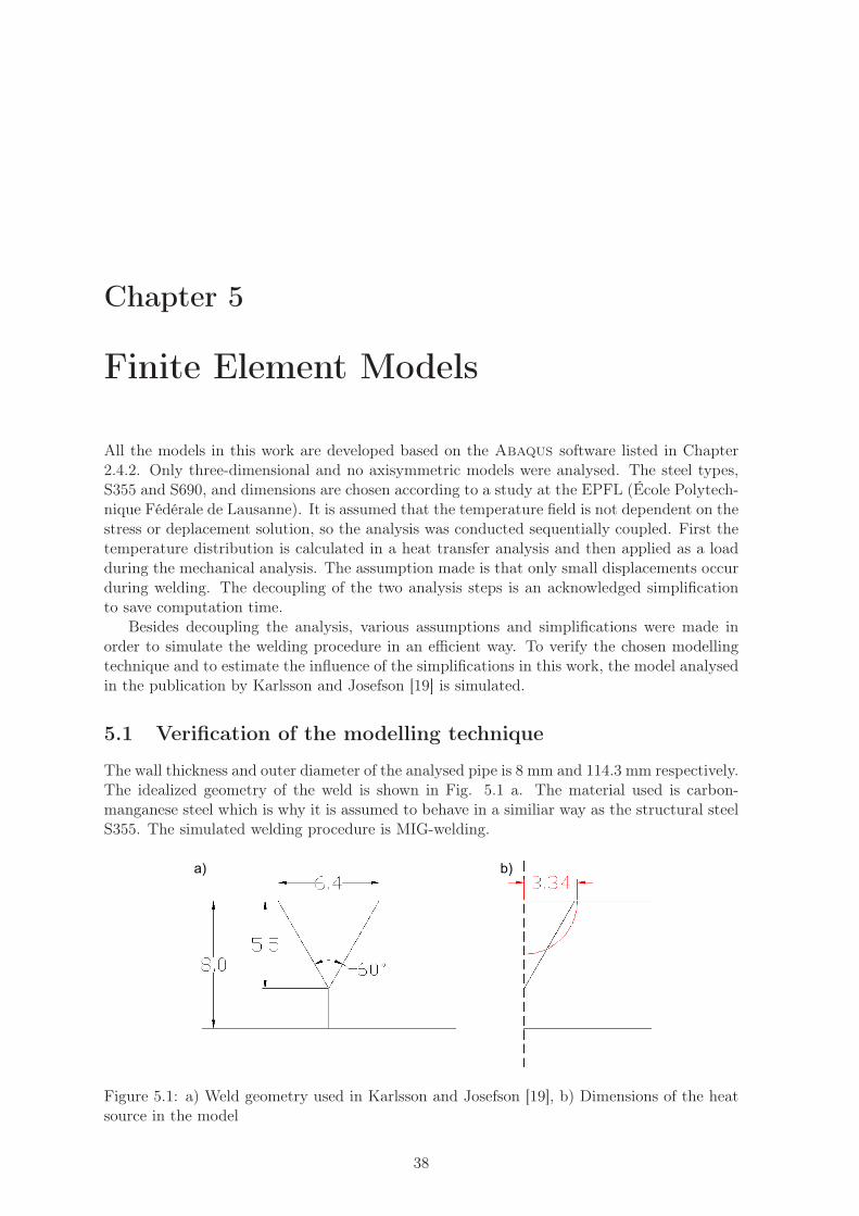
The wall thickness and outer diameter of the analysed pipe is 8 mm and 114.3 mm respectively.The idealized geometry of the weld is shown in Fig. 5.1 a. The material used is carbon-manganese steel which is why it is assumed to behave in a similiar way as the structural steelS355. The simulated welding procedure is MIG-welding.
Figure 5.1: a) Weld geometry used in Karlsson and Josefson [19], b) Dimensions of the heatsource in the model
38

CHAPTER 5. FINITE ELEMENT MODELS 39
In the publication the filler material was modeled. In this work it is assumed that baseand filler metal are the same. The weld itself is not modeled, but the isothermal curves withtemperatures above the melting point define the weld zone. The temperature dependent curvesfor the base metal material properties that are used in the verification model are taken fromKarlsson and Josefson [19] and presented in Fig. 5.2 and 5.3. Note that the conductivityfor temperatures above the melting point is multiplied by three to account for convectionand stirring in the weld pool. The latent heat during solid liquid phase transformation wasincluded with 272 kJ/kg Siddique [38].
Figure 5.2: Thermal material data used in Karlsson and Josefson [19] for the base metal
Figure 5.3: Mechanical material data used in Karlsson and Josefson [19] for the base metal
To save computation time and according to the model chosen by Karlsson and Josefson[19], only half of the pipe relative to the weld line is modeled. A dense mesh in the weldvicinity and the heat affected zone is realized. In the weld zone, the thickness is modeled byfive elements whereas it descends to three elements over the thickness in the parts locatedfurther away. This leads to a number of almost 32000 elements for the entire model. The samemesh with linear continuum elements is used for the thermal and the mechanical analysis.
The heat input is modeled by a constantly moving quarter of a sphere with uniformheat density distribution and realized with the user subroutine Dflux. The radius r of thecorresponding sphere is calculated by assuming that the cross section of the weld is equal
CHAPTER 5. FINITE ELEMENT MODELS 40
to the section of a quarter circle with the radius r. For the verification model, this leads tor = 3.34 mm, compare 5.1 b. For the determination of the circular path of the welding source,the center point of the heat source runs on the outside of the tube on the weld center line.According to Karlsson and Josefson [19], the heat input for the symmetric model is 630 kJ/mand the welding arc is moving at 6.0 mm/s. As mentionend in chapter 4.1.3, the arc efficiencycan only be approximated and here a value as high as 90 % was assumed.
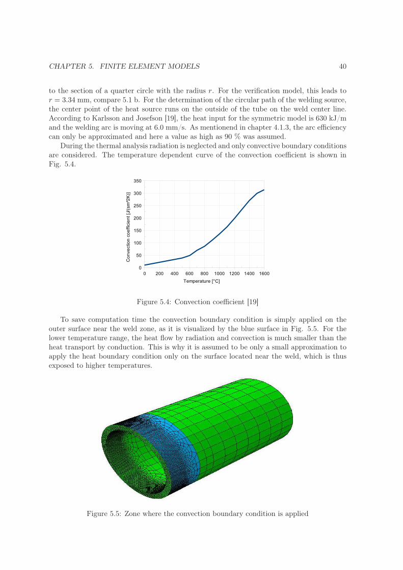
During the thermal analysis radiation is neglected and only convective boundary conditionsare considered. The temperature dependent curve of the convection coefficient is shown inFig. 5.4.
Figure 5.4: Convection coefficient [19]
To save computation time the convection boundary condition is simply applied on theouter surface near the weld zone, as it is visualized by the blue surface in Fig. 5.5. For thelower temperature range, the heat flow by radiation and convection is much smaller than theheat transport by conduction. This is why it is assumed to be only a small approximation toapply the heat boundary condition only on the surface located near the weld, which is thusexposed to higher temperatures.
Figure 5.5: Zone where the convection boundary condition is applied

CHAPTER 5. FINITE ELEMENT MODELS 41
Because of the use of symmetry, no heat flux occurs across the symmetry surface. Fig.5.6 shows the temperature distribution during the welding procedure, when the arc reaches270° in circumferential direction. Fig. 5.7 shows the isothermes in thickness direction of thepipe. The molten area is colored in red and the actual weld is symbolized with bold blacklines. With the assumptions made about the geometry of the heat source, the isothermes thatdefine the weld geometry envelop a larger surface than the actual weld. The penetration ismodeled almost realistic whereas the thickness of the weld on the surface is overestimated.
Figure 5.6: Temperature distribution during the welding process of the verification model
Figure 5.7: Temperature distribution and weld geometry of the verification model
For the mechanical analysis, the nodal temperature histories calculated during the thermalanalysis is applied as thermal loads. The mechanical boundary conditions have also to accountfor the symmetry, as it is shown in Fig.4.10. After the analysis, the calculated residual stressdistribtion is compared to the experimental results and the analytical solution pulished in thereference article [19]. The calculation time for the thermal and the mechanical analysis is 23and 27 hours respectively.
Fig. 5.8 shows the hoop and the axial stress distribution on the outer surface of the pipeat 150° in circumferential direction. Both stress distributions calculated in the simulationshow the same tendency as the experimental data and the analytical solution.

CHAPTER 5. FINITE ELEMENT MODELS 42
Figure 5.8: Hoop and axial stress distribution at 150° on the outer surface of the verificationmodel
By comparing the axial stress distribution on the outer and inner surface at 150° (Fig.5.9), it can be noted, that the stresses are opposed and thus create a bending moment, whichis a typical stress distribution for welded pipes.
Figure 5.9: Axial stress distribution at 150° on the outer and inner surface of the verificationmodel
In conclusion, the simulation technique seems adequate to obtain a realistic stress dis-tribution for the simulated weld even though the chosen geometry of the heat source doesnot create the desired weld shape. For the following models the influence of the mechanicalmaterial data and the number of weld passes on the residual stress field was investigated byusing the same simplifications as for the verification model.
5.2 Comparison of the different models
For the thermal analysis many input parameters are needed, such as the temperature depen-dent material properties, the boundary conditions as convection and radiation as well as thewelding parameters. In this work, the principle welding parameters of heat input and weldingspeed could not be measured because no experimental welding procedure was conducted. ForMAG-welding the heat input can be between five and 100 kJ/s and the welding speed can

CHAPTER 5. FINITE ELEMENT MODELS 43
be as high as 25 mm/s [34]. Due to this large range of possible input parameters, after aniterative procedure, a heat input of 13.8 kW was chosen which leads to a volumetric heat flowof 5 kW/mm3. Because of the large weld volume, a welding speed as slow as 1.5 mm/s wasestimated to be a realistic value.
For the paramteric study ten models were calculated as listed in Tab. 5.1. For a betteroverview the multipass models are highlighted in grey. The aim of the parametric study, isto compare the influence on the residual stress field of the mechanical material data and thenumber of simulated weld passes. For the study on the influence of the mechanical materialdata, first single-pass and multi-pass models of the two different steel grades (M1 vs. M2, andM3 vs. M4) are studied. Additionally, single-pass models using the yield strength or/and theYoung’s modulus deduced from the test results in Chapter 3 are developed and compared tothe models with the Eurocode 3 data (M1 vs. M5, M6, M7 and M2 vs. M8, M9, M10). Themodels M5, M6, M7 and M8 are used in order to study the independent effects of the yieldstrength and the Young’s modulus. Therefore in models M5 and M7, the Young’s modulus ofthe test results and the yield strength of the Eurocode 3 is used. Conversely, in the modelsM6 and M8 the data for the Young’s modulus is chosen from the Eurocode and the yieldstrength from the experimental part.
Model n° Parameter studied n° of Material Yield Young’sweld passes strength modulus
M1 Material 1 S355 EC3 EC3M2 Multi-pass 3 S355 EC3 EC3M3 Material 1 S690 EC3 EC3M4 Material / Multi-pass 3 S690 EC3 EC3M5 Young’s modulus 1 S355 EC3 testsM6 Yield strength 1 S355 tests EC3M7 Material (test data) 1 S355 tests testsM8 Young’s modulus 1 S690 EC3 testsM9 Yield strength 1 S690 tests EC3M10 Material (test data) 1 S690 tests tests
Table 5.1: Parametric study
The diameter and wall thickness of the analysed tubes is 193.4 mm and 20 mm respectively.The dimensions of the welded tube, the shape of the weld passes for the multipass model, andthe welding direction of the different passes are presented in Fig. 5.10.
According to the Eurocode 3, the thermal material behavior is the same for all the struc-tural steel types. For the mechanical material data, only the data for the yield strengthchanges for the S690 compared to the model with S355. Therefore, the results of the samethermal analysis can be used for both steel types and only two thermal analyses were con-ducted for the ten models. For the simulation of the multi-pass model the total heat inputand the welding speed is defined the same as for the single-pass model. The geometry for theweld was chosen according to the regulations in DIN9692-1 [16]. Its approximation by thesingle-pass and the multi-pass model is shown in Fig. 5.11.
For the calculation of the weld shape, it was assumed that the multi-pass weld coversapproximately the same welding volume as the assumed single-pass weld. The heat inputfor the three different passes in the multi-pass model was calculated based on the surfacethat each weld pass covers as it is illustrated in Fig. 5.11. This leads to a heat input of 3.4

CHAPTER 5. FINITE ELEMENT MODELS 44
0°
270° 90°
180°
2nd
and 3rd
pass
1st
pass
Start/End position
20
153.4
20
Figure 5.10: Dimensions of the welded tube, shape of the weld and welding direction of eachpass
Figure 5.11: Assumed weld geometry for the different models
Figure 5.12: Heat source shape for the single-pass a) and multi-pass b) weld
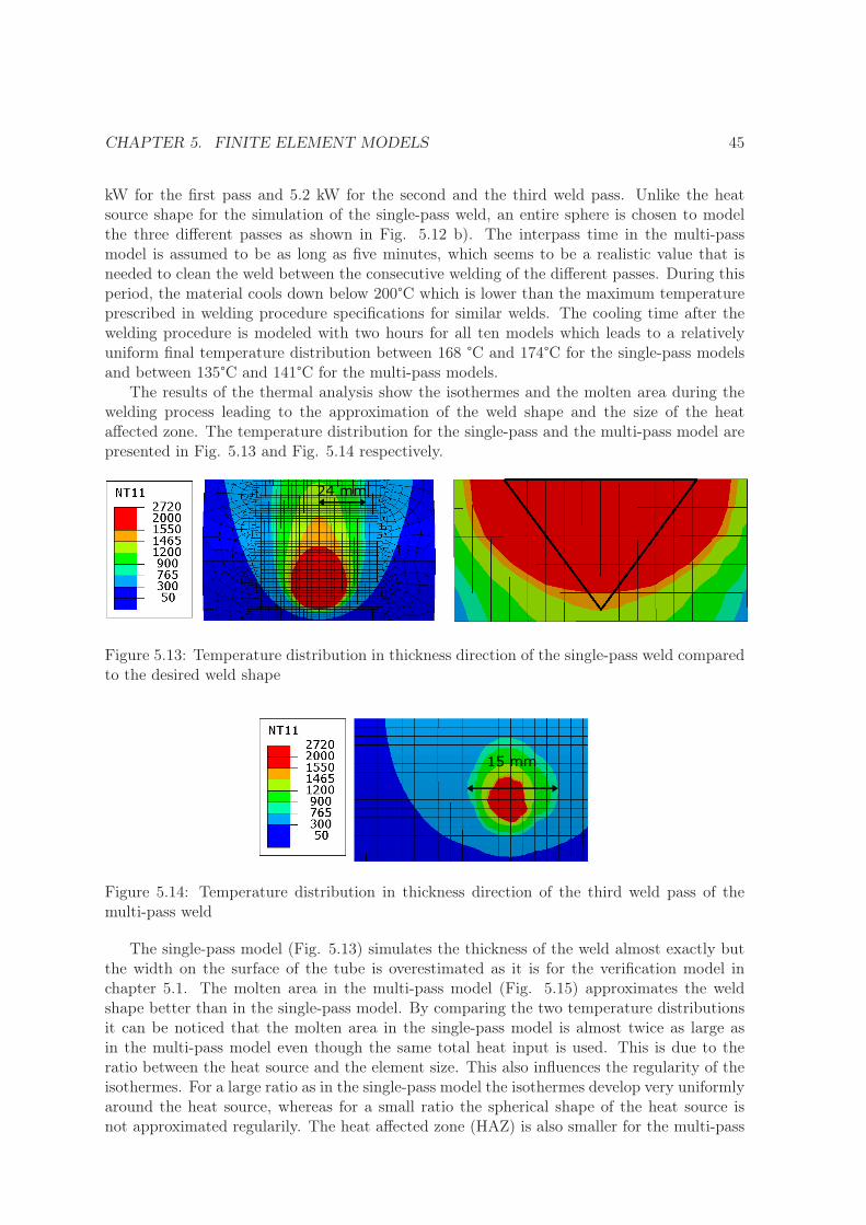
CHAPTER 5. FINITE ELEMENT MODELS 45
kW for the first pass and 5.2 kW for the second and the third weld pass. Unlike the heatsource shape for the simulation of the single-pass weld, an entire sphere is chosen to modelthe three different passes as shown in Fig. 5.12 b). The interpass time in the multi-passmodel is assumed to be as long as five minutes, which seems to be a realistic value that isneeded to clean the weld between the consecutive welding of the different passes. During thisperiod, the material cools down below 200°C which is lower than the maximum temperatureprescribed in welding procedure specifications for similar welds. The cooling time after thewelding procedure is modeled with two hours for all ten models which leads to a relativelyuniform final temperature distribution between 168 °C and 174°C for the single-pass modelsand between 135°C and 141°C for the multi-pass models.
The results of the thermal analysis show the isothermes and the molten area during thewelding process leading to the approximation of the weld shape and the size of the heataffected zone. The temperature distribution for the single-pass and the multi-pass model arepresented in Fig. 5.13 and Fig. 5.14 respectively.
Figure 5.13: Temperature distribution in thickness direction of the single-pass weld comparedto the desired weld shape
Figure 5.14: Temperature distribution in thickness direction of the third weld pass of themulti-pass weld
The single-pass model (Fig. 5.13) simulates the thickness of the weld almost exactly butthe width on the surface of the tube is overestimated as it is for the verification model inchapter 5.1. The molten area in the multi-pass model (Fig. 5.15) approximates the weldshape better than in the single-pass model. By comparing the two temperature distributionsit can be noticed that the molten area in the single-pass model is almost twice as large asin the multi-pass model even though the same total heat input is used. This is due to theratio between the heat source and the element size. This also influences the regularity of theisothermes. For a large ratio as in the single-pass model the isothermes develop very uniformlyaround the heat source, whereas for a small ratio the spherical shape of the heat source isnot approximated regularily. The heat affected zone (HAZ) is also smaller for the multi-pass

CHAPTER 5. FINITE ELEMENT MODELS 46
Figure 5.15: Temperature distribution in thickness direction of the multi-pass weld comparedto the desired weld shape

CHAPTER 5. FINITE ELEMENT MODELS 47
model than for the single-pass model.For the development of residual stresses, the time period that the material needs to cool
from 800°C to 500°C is mandatory, because it can be used to approximate the microstructurethat is reached during the cooling process. In many publications this time period is referredto as t8/5. To obtain this value in the output data of an Abaqus model, history output hasto be calculated. Even if this history output is only requested for a limited number of points,a long computation time is needed. This is the reason history output was only requested forthe single-pass model and only for four significant points at 0°, 90°, 180°, and 270° in the weldcenter line. The temperature development versus the time is presented in Fig. 5.16.
Figure 5.16: Temperature development in four points located in the weld center line
Fig. 5.16 shows that the temperature history is uniform in the weld center line except forthe start-end position because the material in this zone is heated twice. This leads also toa different residual stress distribution which is why the following paragraphs focus partiallyon the stress distribution at the start-end position. A physical error can be noticed whencomparing the temperature development at 270° and at 0°. At approximately 750°C, thetemperature at 0° drops below the temperature at 270°. This error can be attributed to thesimplification of the convective and radiative boundary conditions, that underestimate thecooling rate when an almost uniform temperature distribution is reached in the tubes and theheat starts to flow back to the weld region, because only in this section can heat be releasedto the surroundings.
The radial stresses are negligible compared to the stresses in axial and circumferentialdirection. Therefore, the radial stresses are not analysed in this work. The following diagramsshow the significant stress distributions of the different models. More stress curves can befound in the appendix A. First, the results for the two different steel types with the materialdata from the Eurocode 3 [11] will be compared.
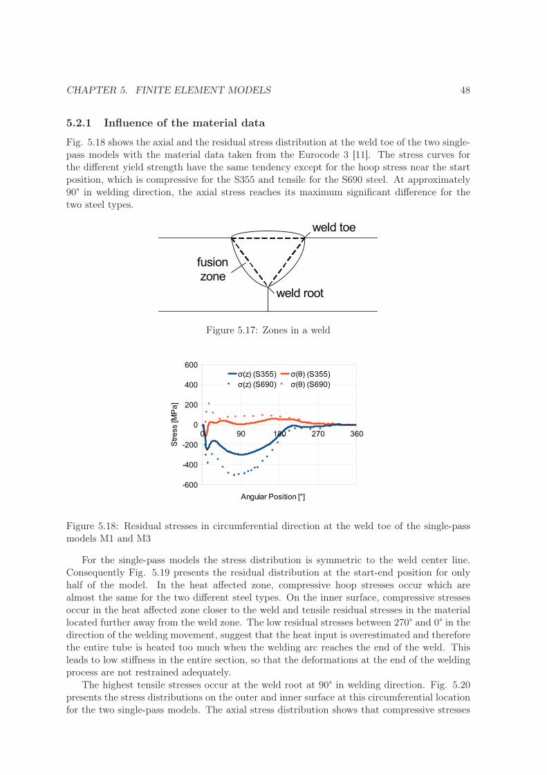
CHAPTER 5. FINITE ELEMENT MODELS 48
5.2.1 Influence of the material data
Fig. 5.18 shows the axial and the residual stress distribution at the weld toe of the two single-pass models with the material data taken from the Eurocode 3 [11]. The stress curves forthe different yield strength have the same tendency except for the hoop stress near the startposition, which is compressive for the S355 and tensile for the S690 steel. At approximately90° in welding direction, the axial stress reaches its maximum significant difference for thetwo steel types.
weld toe
weld root
fusion zone
Figure 5.17: Zones in a weld
Figure 5.18: Residual stresses in circumferential direction at the weld toe of the single-passmodels M1 and M3
For the single-pass models the stress distribution is symmetric to the weld center line.Consequently Fig. 5.19 presents the residual distribution at the start-end position for onlyhalf of the model. In the heat affected zone, compressive hoop stresses occur which arealmost the same for the two different steel types. On the inner surface, compressive stressesoccur in the heat affected zone closer to the weld and tensile residual stresses in the materiallocated further away from the weld zone. The low residual stresses between 270° and 0° in thedirection of the welding movement, suggest that the heat input is overestimated and thereforethe entire tube is heated too much when the welding arc reaches the end of the weld. Thisleads to low stiffness in the entire section, so that the deformations at the end of the weldingprocess are not restrained adequately.
The highest tensile stresses occur at the weld root at 90° in welding direction. Fig. 5.20presents the stress distributions on the outer and inner surface at this circumferential locationfor the two single-pass models. The axial stress distribution shows that compressive stresses

CHAPTER 5. FINITE ELEMENT MODELS 49
Figure 5.19: Residual stresses at the start-end position of the single-pass models M1 and M3
occur on the outside and tensile stresses on the inside of the tube, which creates a bendingmoment in the pipe. For the steel type S355, the stresses on the outside and the inside surfaceare almost exactly opposed. The axial stresses resulting from the simulation of steel type S690are almost twice as high on the weld root and on the weld toe compared to the results ofS355, whereas in the parts outside of the heat affected zone the stresses coincide. Accordingto Radaj [35] the residual stress distribution in the entire welded component is linked to theplastic deformation in the weld zone. Thus, the stresses in the far field are not caused bythermal plastic strains but they are due to kinematic compatibilty.
Figure 5.20: Residual stresses at 90° of the single-pass models M1 and M3
Fig. 5.21 presents the residual stresses in circumferential direction at the weld toe of themulti-pass models. The figure on the left shows the stress distribution on the weld toe locatedon the second weld pass and the figure on the right the stress distribution on the third weldpass respectively. The tendency of the stress distributions is the same at the two locations, butthe magnitude and sign differ. In detail, the axial residual stress near the second weld pass istensile in the first half of the tube in circumferential direction, whereas it is compressive nearthe third weld pass. The axial stress distribution of the two different steel types is similar,while on the contrary, the S690 model produced higher tensile hoop stresses than the modelwith tubes made of S355.
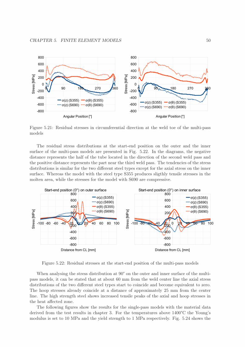
CHAPTER 5. FINITE ELEMENT MODELS 50
Figure 5.21: Residual stresses in circumferential direction at the weld toe of the multi-passmodels
The residual stress distributions at the start-end position on the outer and the innersurface of the multi-pass models are presented in Fig. 5.22. In the diagrams, the negativedistance represents the half of the tube located in the direction of the second weld pass andthe positive distance represents the part near the third weld pass. The tendencies of the stressdistributions is similar for the two different steel types except for the axial stress on the innersurface. Whereas the model with the steel type S355 produces sligthly tensile stresses in themolten area, while the stresses for the model with S690 are compressive.
Figure 5.22: Residual stresses at the start-end position of the multi-pass models
When analysing the stress distribution at 90° on the outer and inner surface of the multi-pass models, it can be stated that at about 60 mm from the weld center line the axial stressdistributions of the two different steel types start to coincide and become equivalent to zero.The hoop stresses already coincide at a distance of approximately 25 mm from the centerline. The high strength steel shows increased tensile peaks of the axial and hoop stresses inthe heat affected zone.
The following figures show the results for the single-pass models with the material dataderived from the test results in chapter 3. For the temperatures above 1400°C the Young’smodulus is set to 10 MPa and the yield strength to 1 MPa respectively. Fig. 5.24 shows the

CHAPTER 5. FINITE ELEMENT MODELS 51
Figure 5.23: Residual stresses at 90° of the multi-pass models
stress distribution at the weld toe of different models for steel grade S355. The maximumdeviation occurs for the hoop stress of model M6, where only the yield strength is changed,compared to the model with the Eurocode data. The influence of the Young’s modulusfrom the test data reaches its maximum also in the hoop stress distribution, but it is lesspronounced than for model M6. When combining the models M5 and M6, the tendencyof the stress distributions remains the same for the model with the Eurocode data with amaximum deviation of 50 MPa.
Figure 5.24: Residual stresses in circumferential direction at the weld toe of the single-passmodels M1, M5, M6 and M7
Fig. 5.25 illustrates the residual stress distributions at the weld toe for the single-passmodels with the steel grade S690. The tendency of the axial stress remains unchanged andthe maximum derivation occurs for the model where only the Young’s modulus is adapted tothe test results. The tendency of the hoop stress distribution differs for the model M8, butthe hoop stress in general is very low.
In conclusion it can be stated that the yield strength has a significant influence on themagnitude of the stresses in the heat affected zone but not on the general tendency of thestress distribution. The most significant difference that occured for the stress calculationbetween the two different steel types is presented in Fig. 5.18. The hoop stress near the start

CHAPTER 5. FINITE ELEMENT MODELS 52
Figure 5.25: Residual stresses in circumferential direction at the weld toe of the single-passmodels M3, M8, M9 and M10
position is tensile for the high strength steel and compressive for the S355. The calculation ofthe stresses with one steel type therefore does not allow conclusions on the stress distributionfor models with a different yield strength. The mechanical data for steel at high temperaturesgiven in the EC 3 is meant to be used for fire design and underestimates the yield strengthin particular. For a realistic residual stress determination using numerical simulation it istherefore important to use an adequate material model with accurate data for the materialbehavior at high temperatures. The models with the Young’s modulus and the yield strengthfrom the experimental part of this work presented in Figures 5.24 and 5.25 also show theinfluence of the Young’s modulus. It also appears, that the test data for the steel grade S690has a stronger influence on the stress distributions than the test data for the steel grade S355.This could be interpretated as an indicator for the necessity of including the effect of phasetransformation for the steel grade S690 as concluded by Wichers [47].
5.2.2 Influence of the weld-pass number
The following diagrams illustrate the difference between the use of a single-pass and a multi-pass model. The axial stress distribution at the weld toe of the single-pass model differsconsiderably from the axial stress distribution in circumferential direction of the multi-passmodel (compare Fig. 5.26). Except at the start/end position no paralels can be found. Thesame statement is valid for the hoop stress distribution in circumferential direction at theweld toe. Whereas almost no hoop stresses are calculated by the single-pass model, in themulti-pass model, hoop stresses of the magnitude close to the yield strength occur betweenaproximately 40° and 120° in circumferential direction.
The left diagram in fig. 5.27 illustrates the residual stress distribution in the start/endposition on the outer surface. The axial stress distribution on the outer surface of the single-pass and multi-pass model coincides neither in tendency nor in magnitude, whereas the hoopstress distribution on the outer surface shows the same tendeny in both models. The onlyconvergences can be stated for the axial stress distribution on the inner surface in the moltenarea (compare the right diagram in Fig. 5.27).
Fig. 5.28 illustrates the axial and hoop stress distribution at 90° in circumferential direc-tion. The stress distributions of the single-pass and multi-pass model show the same tendencybut differ in magnitude. The stresses on the inside of the tubes at the heat affected zone cal-
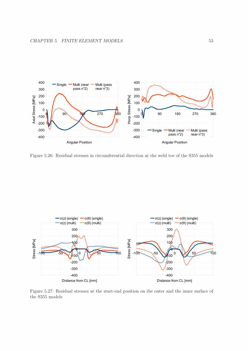
CHAPTER 5. FINITE ELEMENT MODELS 53
Figure 5.26: Residual stresses in circumferential direction at the weld toe of the S355 models
Figure 5.27: Residual stresses at the start-end position on the outer and the inner surface ofthe S355 models
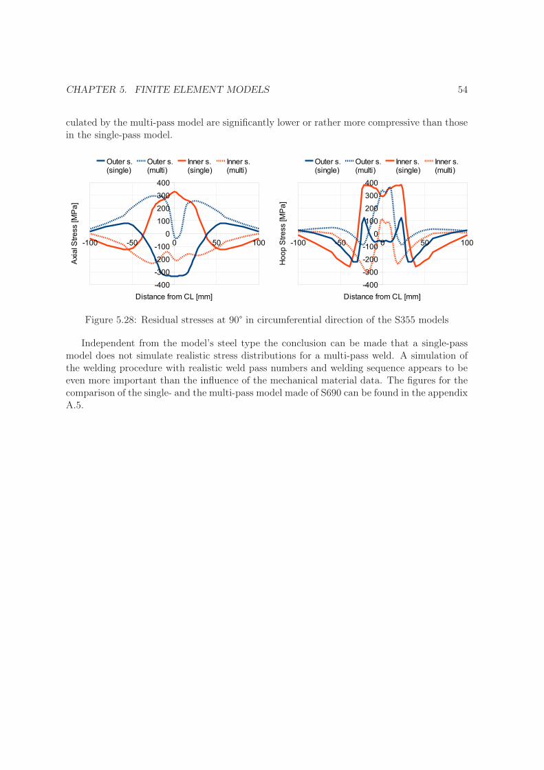
CHAPTER 5. FINITE ELEMENT MODELS 54
culated by the multi-pass model are significantly lower or rather more compressive than thosein the single-pass model.
Figure 5.28: Residual stresses at 90° in circumferential direction of the S355 models
Independent from the model’s steel type the conclusion can be made that a single-passmodel does not simulate realistic stress distributions for a multi-pass weld. A simulation ofthe welding procedure with realistic weld pass numbers and welding sequence appears to beeven more important than the influence of the mechanical material data. The figures for thecomparison of the single- and the multi-pass model made of S690 can be found in the appendixA.5.

Chapter 6
Conclusion
In this work, the welding process and the resulting residual stress field for butt-welded tubesare studied. The aim is to simplify the model in order to save computation time, to study theinfluence of the mechanical material data on the residual stress distribution and the differencebetween a single- and a multi-pass model.
The welding simulation is realized with the finite element software Abaqus. Based on theliterature study it was decided to implement exclusively three-dimensional models, becauseaxi-symmetric models have proven in the past to be not realistic enough for the calculationof the residual stress distribution. For the simulation it is necessary to make assumptionsin order to simplify the model and to reduce the calculation time. The correctness of thesesimplifications have a distinct influence on the quality of the results and are therefore listedbelow:
• No filler material is modeled and the material in the weld pool is assumed to be thesame as the base metal.
• The welding arc is assumed to act on the material like a volumetric heat source withuniform density distribution.
• A constant weld speed is modeled.
• Electro-magnetic and electro-kinetic effects of the welding arc are neglected.
• No fluid flow in the weld pool is taken into consideration.
• The thermal boundary conditions are only applied on the outer surface of the tubesclose to the weld.
Because no experimental welding procedure is part of the work the welding parameters areestimated which might also have an impact on the accuracy of the results. Especially for thesingle-pass model the chosen heat input leads to an important overestimation of the weld size.For further work an experimental welding procedure can provide more accurate parametersand lead to a realistic modeling. This is the reason why it is recommended to measure thewelding paremeters and the temperature history at different locations previous to a weldingsimulation. As the molten area is simulated to large but not deep enough, especially for thesingle-pass model, a Gauss distribution could lead to a more precise simulation. However, thespherical shape of the weld source appears to be an adequate simplification. The applicationsurface of the thermal boundary conditions, on the contrary, seems to be choosen to small.
55

CHAPTER 6. CONCLUSION 56
This is concluded from the final temperature distribution and the variation of the coolingperiods at different locations in the weld.
Furthermore, not only the welding process is simplified in this work, but also the materialmodel is realized under the following assumptions:
• Both steel types have the same thermal material properties,
• The material is assumed to behave non-viscously even at high temperatures.
• A bilinear stress-strain curve is used for the material model at all temperatures.
• No effects of microstructural transformations are taken into consideration.
The bilinear stress-strain behavior is the most simplified material model for metals includ-ing plasticiy. It is more realistic to include hardening. Furthermore, steel behaves viscous athigh temperatures. Accoring to the literature study it also is essential to include the effectsof microstructural phase transformations, especially for high strength steel. The accuracy ofthe results might therefore have been influenced by the correctness of the material model. Forfurther research, it is recommended to study the influence of a more realistic material modeland to include phase transformation effects.
The accuracy of the employed material data is a major factor for the realistic description ofthe welding process. Therefore, the research of the thermal and especially mechanical materialdata at elevated temperatures of the steel grades S355 and S690 is another focus in this work.Not only the availability of the data in the high temperature range, but also the scatter dueto manufacturing and differing test set-up has an important influence on the results. For thecommon construction steel type S355 a comprehensive study is conducted by Wichers [47].For the high strength steel grade S690 only information on the mechanical behavior in thehigh temperature range is published [29]. The Eurocode 3 [11] provides thermal materialdata as well as temperature dependent reduction factors for the Young’s modulus and theyield strength. It is valid for numerous different steel types and therefore considers the samematerial properties for the two steel types used in this work.
To verify the data provided by the literature, tensile tests at three different temperatures(20°C, 250°C and 800°C) are conducted in order to obtain the stress-strain curves. Based onthese results, the Young’s modulus and the yield strength are calculated. The results for thetests at elevated temperatures are in agreement with the data found in the literature and inEurocode 3 for fire design of steel structures [11] except for the Young’s modulus of the steelgrade S355 at 800°C which is underestimated by the European standard. As for the resultsat room temperature, the average value of the experimental results show approximately 20% higher results for the yield strength than the consulted standard. The Eurocode uses a5%-factile which is on the safe side for fire contsruction, but not automatically for the residualstress calculation.
The obtained mechanical data are then used as input data for the mechnical analysis ofa singlepass model and compared to the results that are obtained with the data originatingfrom the EC 3. When analysing the residual stress distribution at the weld toe, one cannotice a uniform tendency for all the models. The maximum stress derivation for the modelswith steel grade S355 are 70 MPa and for steel grade S690, 130 MPa respectively. However,the stress distributions for the different steel grades don’t support conclusions from one stressfield on the other because, in the weld and heat affected zone, they differ greatly while inthe far field they coincide. These results leave unanswered whether the two steel grades

CHAPTER 6. CONCLUSION 57
can be simulated with the bilinear material model or if the phase transformation effects canbe neglected especially for the high strength steel. Furthermore, additional tests at varioustemperatures between 250°C and 800°C appear to be beneficial in order to verify the trend ofthe curves given by the Eurocode 3 and to be able to use more realistic material data in thenumerical models.
The analysis regarding the quality of an approximation of a multi-pass weld by a single-pass weld reveals the important influence of the weld pass numbers on the residual stressfield. Mostly, the calculated stress distributions don’t show the same tendency and generallythey differ greatly in magnitude. No significant similarities can be determined. Additionally,the weld pool size is largely overestimated for the single-pass model. Therefore, it can beconcluded that this is an oversimplification and leads to non-realistic results.

Bibliography
[1] C. Acevedo. Influence of residual stresses on fatigue response of welded tubular joints.PhD thesis, Ecole Polytechnique Fédérale de Lausanne (EPFL), 2011.
[2] Z. Barsoum. Residual stress analysis and fatigue assessment of welded steel structures.School of Engineering Sciences, Stockholm, Sweden, 2008.
[3] U. Boese. Das Verhalten der Stähle beim Schweißen - Teil I: Grundlagen. DVS Media,1995.
[4] R. Bonn. Experimentelle und numerische Ermittlung der thermo-mechanischenBeanspruchung des Wurzelbereichs austenitischer Rundnähte. PhD thesis, Materialprü-fungsanstalt Universität Stuttgart, 2002.
[5] S. Brown and H. Song. Finite element simulation of welding of large structures. Journalof engineering for industry, 114(4):441–451, 1992.
[6] D. Deng and S. Kiyoshima. FEM prediction of welding residual stresses in a SUS304girth-welded pipe with emphasis on stress distribution near weld start/end location.Computational Materials Science, 50(2):612–621, December 2010.
[7] D. Deng and H. Murakawa. Prediction of welding residual stress in multi-pass butt-weldedmodified 9Cr-1Mo steel pipe considering phase transformation effects. Computationalmaterials science, 37(3):209–219, 2006.
[8] D. Deng and H. Murakawa. Numerical simulation of temperature field and residual stressin multi-pass welds in stainless steel pipe and comparison with experimental measure-ments. Computational materials science, 37(3):269–277, 2006.
[9] P. Dong. On the mechanics of residual stresses in girth welds. Journal of pressure vesseltechnology, 129:345, 2007.
[10] I. F.Z. Fanous, M. Y.A. Younan, and A. S. Wifi. Introduction of the element interactiontechnique for welding analysis and simulation. Journal of pressure vessel technology, 127:487, 2005.
[11] Normenausschuss Bauwesen (NABau) Deutsches Institut für Normung e.V. Eurocode 3:Bemessung und Konstruktion von Stahlbauten - Teil 1-2: Allgemeine Regeln - Tragwerks-bemessung für den Brandfall, 2006.
[12] Normenausschuss Bauwesen (NABau) Deutsches Institut für Normung e.V. Eurocode 3:Bemessung und Konstruktion von Stahlbauten - Teil 1-9: Ermüdung, 2006.
58

BIBLIOGRAPHY 59
[13] Normenausschuss Bauwesen (NABau) Deutsches Institut für Normung e.V. Eurocode3: Bemessung und Konstruktion von Stahlbauten - Teil 1-12: Zusätzliche Regeln zurErweiterung von EN 1993 auf Stahlsorten bis S700, 2007.
[14] Normenausschuss Materialprüfung (NMP) Deutsches Institut für Normung e.V. Met-allische Werkstoffe - Zugversuch - Teil 5: Prüfverfahren bei erhöhter Temperatur, 1992.
[15] Normenausschuss Materialprüfung (NMP) Deutsches Institut für Normung e.V. Met-allische Werkstoffe - Zugversuch - Teil 1: Prüfverfahren bei Raumtemperatur, 2001.
[16] Normenausschuss Schweißtechnik (NAS ) Deutsches Institut für Normung e.V.Schweißen und verwandte Prozesse - Empfehlungen zur Schweißnahtvorbereitung - Teil1: Lichtbogenhandschweißen, Schutzgasschweißen, Gasschweißen, WIG-Schweißen undStrahlschweißen von Stählen (ISO 9692Â1:2003), 2004.
[17] J. A. Goldak and M. Akhlaghi. Computational welding mechanics. Springer Verlag, 2005.
[18] J. Hildebrand. Numerische Schweißsimulation - Bestimmung von Temperatur, Gefügeund Eigenspannung an Schweißverbindungen aus Stahl- und Glaswerkstoffen. PhD thesis,Institut für Stahlbau, Bauhausuniversität Weimar, 2008.
[19] R. I. Karlsson and B. L. Josefson. Three-dimensional finite element analysis of tempera-tures and stresses in a single-pass butt-welded pipe. Journal of pressure vessel technology,112:76, 1990.
[20] U. Kuhlmann, J. Bergmann, A. Dürr, R. Thumser, H. P. Günther, and U. Gerth. Er-höhung der Ermüdungsfestigkeit von geschweißten höherfesten Baustählen durch Anwen-dung von Nachbehandlungsverfahren. Stahlbau, 74(5):358–365, 2005. ISSN 1437-1049.
[21] C. H Lee and K. H Chang. Three-dimensional finite element simulation of residualstresses in circumferential welds of steel pipe including pipe diameter effects. MaterialsScience and Engineering: A, 487(1-2):210–218, 2008.
[22] Chin-Hyung Lee and Kyong-Ho Chang. Prediction of residual stresses in high strengthcarbon steel pipe weld considering solid-state phase transformation effects. Computers& Structures, 89(1-2):256–265, January 2011.
[23] L. E. Lindgren. Finite element modeling and simulation of welding part 1: Increasedcomplexity. Journal of thermal stresses, 24(2):141–192, 2001.
[24] L. E. Lindgren. Finite element modeling and simulation of welding - part 2: improvedmaterial modeling. Journal of thermal stresses, 24(3):195–231, 2001.
[25] L. E. Lindgren. Finite element modeling and simulation of welding - part 3: efficiencyand integration. Journal of thermal stresses, 24(4):305–334, 2001.
[26] L. Lobanov, V. Poznyakov, V. Pivtorak, O. Mikhodui, and V. Orlovskyi. Residual stressesin welded joints of high-strength steels. Materials Science, pages 1–11, 2009.
[27] T. Loose. Einfluß des transienten Schweißvorganges auf Verzug, Eigenspannungen undStabilitätsverhalten axial gedrückter Kreiszylinderschalen aus Stahl. PhD thesis, Univer-sität Fridericiana Karlsruhe (TH), 2007.

BIBLIOGRAPHY 60
[28] J. Mullins and J. Gunnars. Influence of Hardening Model on Weld Residual Stress Dis-tribution. Swedish Radiation Safety Authority, 2009.
[29] J. Outinen. Mechanical properties of structural steel at elevated temperatures and aftercooling down. Interscience Communications, 2007.
[30] U. Peil and M. Wichers. Schweißen unter Betriebsbeanspruchung - Werkstoffkennwertefür einen S 355 J2G3 unter Temperaturen bis 1200° C. Stahlbau, 73(6):400 – 415, 2004.
[31] U. Peil and M. Wichers. Schweißen unter Betriebsbeanspruchung - Werkstoffkennwertezur Temperaturfeldberechnung für einen S 355 J2 G3. Stahlbau, 74(4):249 – 257, 2005.
[32] U. Peil and M. Wichers. Schweißen unter Betriebsbeanspruchung - Numerische undexperimentelle Bestimmung des Temperaturfeldes beim Schweißen. Stahlbau, 74(11):843–851, 2005.
[33] Dieter Radaj. Heat effects of welding : temperature field, residual stress, distortion.Springer, 1992.
[34] Dieter Radaj. Schweißprozeßsimulation : Grundlagen und Anwendungen. FachbuchreiheSchweißtechnik; 141. Verl. für Schweißen und Verwandte Verfahren, DVS-Verl., 1999.
[35] Dieter Radaj. Eigenspannung und Verzug beim Schweißen: Rechen- und Meßverfahren.DVS Media, 2001.
[36] L.O. Raymond and J. Chipman. Thermodynamic functions of iron. Trans. Met. Soc.AIME, 239:630–633, 1967.
[37] F. Richter. Die wichtigsten physikalischen Eigenschaften von 52 Eisenwerkstoffen.Stahleisen - Sonderberichte, 8, 1973.
[38] M. Siddique. Experimental and finite element investigation of residual stresses and dis-tortion in welded pipe and flange joints. PhD thesis, Ghulam Ishaq Khan Institute ofEngineering Sciences and Techonology, 2005.
[39] American Standard. ASTM E21-09 - Standard Test Methods for Elevated TemperatureTension Tests of Metallic Materials, 2009.
[40] American Standard. ASTM E8M-09 - Standard Test Methods for Tension Testing ofMetallic Materials, 2009.
[41] D. Systèmes. Abaqus Analysis User’s Manual. ABAQUS Inc., Dassault Systèmes, France,2007.
[42] D. Tikhomirov, B. Rietman, K. Kose, and M. Makkink. Computing welding distortion:Comparison of different industrially applicable methods. Advanced Materials Research,6-8:195–202, 2005.
[43] F. Schröter U. Kuhlmann, A. Dürr. Hochfeste Feinkornbaustähle im Stahlbau: An-wendung im Stahlbau insbesondere unter Berücksichtigung der Ermüdungsfestigkeitgeschweißter Konstruktionen. Technical report, DVS, 2005.
[44] T. Ummenhofer, I. Weich, and T. Nitschke-Pagel. Lebens- und Restlebensdauerver-längerung geschweißter Windenergieanlagentürme und anderer Stahlkonstruktionendurch Schweißnahtnachbehandlung. Stahlbau, 74(6):412–422, 2005. ISSN 1437-1049.
BIBLIOGRAPHY 61
[45] Normenausschuss Eisen und Stahl (FES). DIN EN 10025 -2: Warmgewalzte Erzeugnisseaus Baustählen - Teil 2: Technische Lieferbedingungen für unlegierte Baustähle, 2005.
[46] M. Volz. Die Rissentstehung in statisch beanspruchten Stahlkonstruktionen unter Berück-sichtigung von Schweißeigenspannung. PhD thesis, Universität Fridericiana Karlsruhe(TH), 2009.
[47] M. Wichers. Schweißen unter einachsiger, zyklischer Beanspruchung - Experimentelle undnumerische Untersuchungen. PhD thesis, Universitätsbibliothek Braunschweig, 2006.
[48] X. K. Zhu and Y. J. Chao. Effects of temperature-dependent material properties onwelding simulation. Computers & Structures, 80(11):967–976, May 2002.
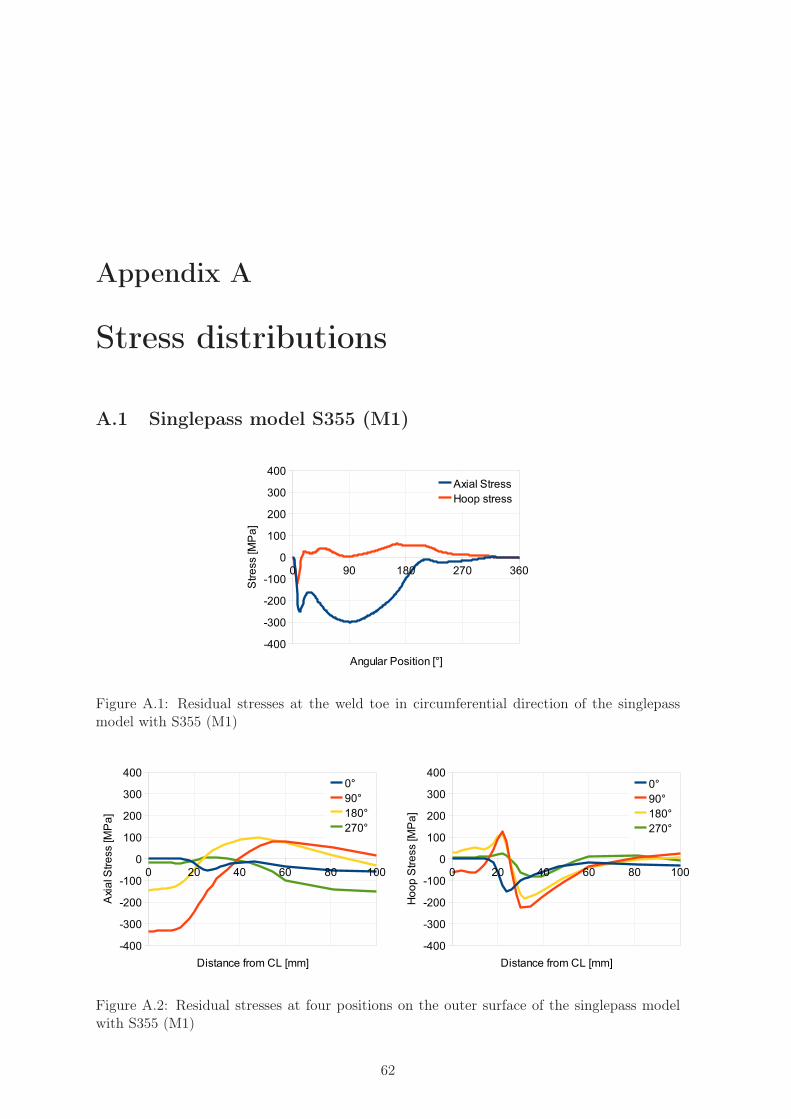
Appendix A
Stress distributions
A.1 Singlepass model S355 (M1)
Figure A.1: Residual stresses at the weld toe in circumferential direction of the singlepassmodel with S355 (M1)
Figure A.2: Residual stresses at four positions on the outer surface of the singlepass modelwith S355 (M1)
62
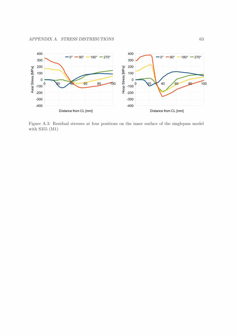
APPENDIX A. STRESS DISTRIBUTIONS 63
Figure A.3: Residual stresses at four positions on the inner surface of the singlepass modelwith S355 (M1)
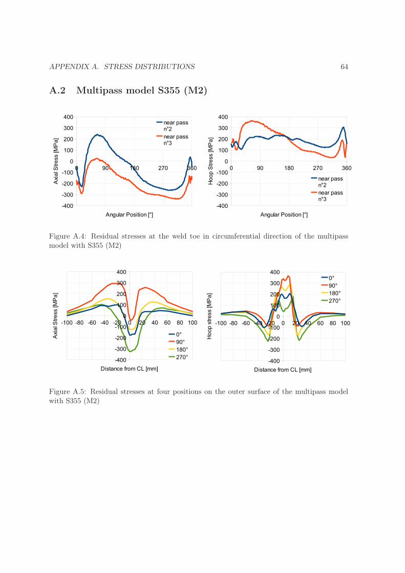
APPENDIX A. STRESS DISTRIBUTIONS 64
A.2 Multipass model S355 (M2)
Figure A.4: Residual stresses at the weld toe in circumferential direction of the multipassmodel with S355 (M2)
Figure A.5: Residual stresses at four positions on the outer surface of the multipass modelwith S355 (M2)

APPENDIX A. STRESS DISTRIBUTIONS 65
Figure A.6: Residual stresses at four positions on the inner surface of the multipass modelwith S355 (M2)
A.3 Singlepass model S690 (M3)
Figure A.7: Residual stresses at the weld toe in circumferential direction of the singlepassmodel with S690 (M3)

APPENDIX A. STRESS DISTRIBUTIONS 66
Figure A.8: Residual stresses at four positions on the outer surface of the singlepass modelwith S690 (M3)
Figure A.9: Residual stresses at four positions on the inner surface of the singlepass modelwith S690 (M3)
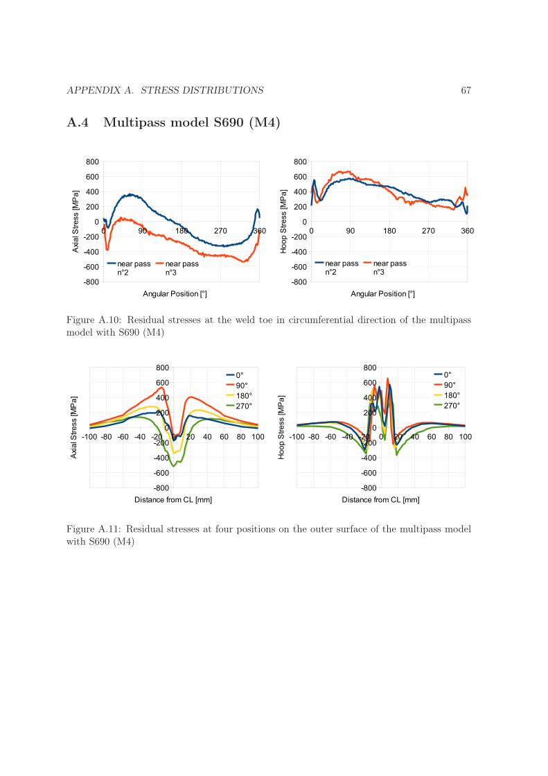
APPENDIX A. STRESS DISTRIBUTIONS 67
A.4 Multipass model S690 (M4)
Figure A.10: Residual stresses at the weld toe in circumferential direction of the multipassmodel with S690 (M4)
Figure A.11: Residual stresses at four positions on the outer surface of the multipass modelwith S690 (M4)

APPENDIX A. STRESS DISTRIBUTIONS 68
Figure A.12: Residual stresses at four positions on the inner surface of the multipass modelwith S690 (M4)
A.5 Single- and multipass model of S690
Figure A.13: Residual stresses in circumferential direction of the S690 models
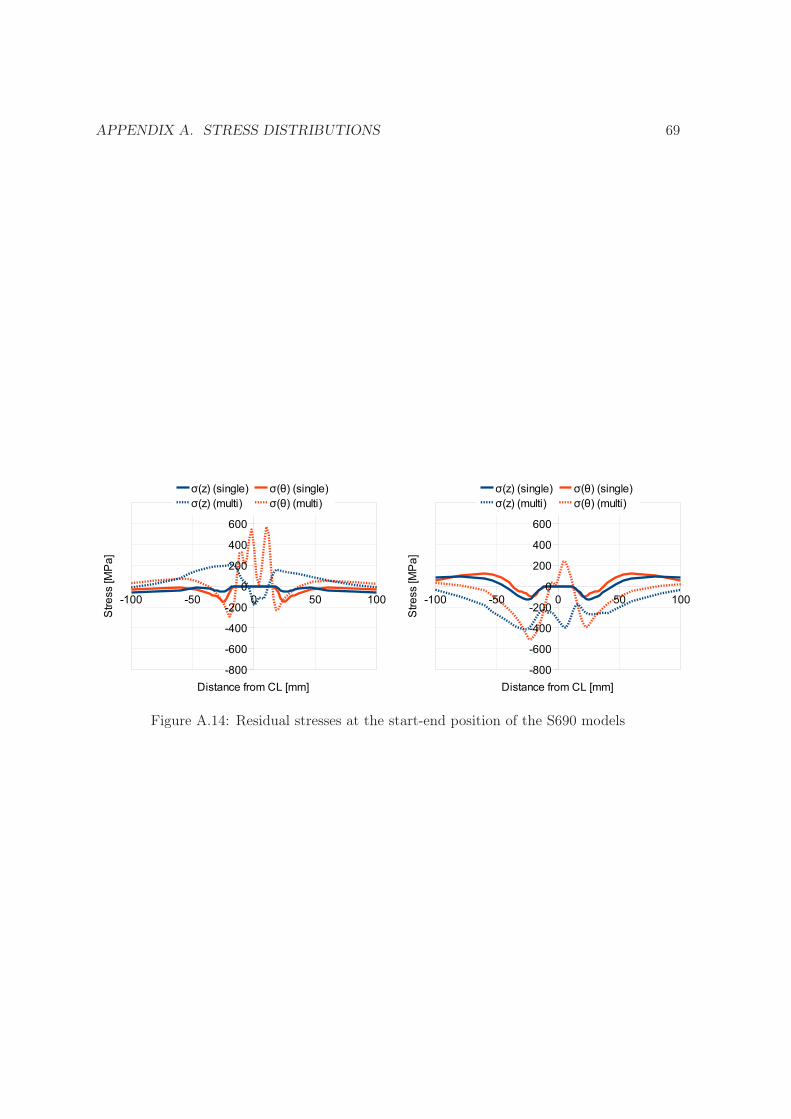
APPENDIX A. STRESS DISTRIBUTIONS 69
Figure A.14: Residual stresses at the start-end position of the S690 models
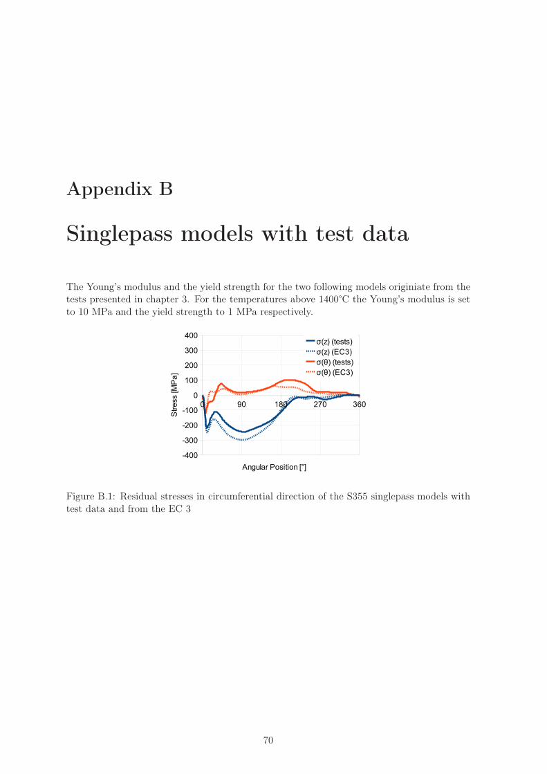
Appendix B
Singlepass models with test data
The Young’s modulus and the yield strength for the two following models originiate from thetests presented in chapter 3. For the temperatures above 1400°C the Young’s modulus is setto 10 MPa and the yield strength to 1 MPa respectively.
Figure B.1: Residual stresses in circumferential direction of the S355 singlepass models withtest data and from the EC 3
70

APPENDIX B. SINGLEPASS MODELS WITH TEST DATA 71
Figure B.2: Residual stresses at the start-end position of the S355 singlepass models with testdata and from the EC 3
Figure B.3: Residual stresses at 90° in circumferential direction of the S355 singlepass modelswith test data and from the EC 3
Figure B.4: Residual stresses in circumferential direction of the S690 singlepass models withtest data and from the EC 3

APPENDIX B. SINGLEPASS MODELS WITH TEST DATA 72
Figure B.5: Residual stresses at the start-end position of the S690 singlepass models with testdata and from the EC 3
Figure B.6: Residual stresses at 90° in circumferential direction of the S690 singlepass modelswith test data and from the EC 3

Appendix C
Fortran Code for the Dflux
subroutine
SUBROUTINE DFLUX(FLUX,SOL,JSTEP,JINC,TIME,NOEL,NPT,COORDS,JLTYP,
1 TEMP,PRESS,SNAME)
c
c subroutine for a single-pass butt weld between the tubes with the
c dimensions:
c diameter = 193.4 mm, thickness = 20 mm
c total heat input: Q=13.8 kW
c FLUX(1) will be passed into the routine as the magnitude of the
c flux specified as part of the element-based or surface-
c based flux definition.
c FLUX(2) dq/dT, the rate of change of the flux with respect to the
c temperature at this point, that is estimated zero in this
c analysis.
c SOL the estimated value of the solution variable at this time
c in this point.
c KSTEP the current step number.
c KINC the current increment number.
c TIME(1) the current value of step time.
c TIME(2) the current value of total time.
c NOEL the element number.
c NPT the integration point number in the element or on the
c element’s surface.
c COORDS the array containing the coordinates of this point.
c JLTYP the flux type.
c TEMP the current value of temperature at this integration point.
c PRESS the current value of the equivalent pressure stress at this
c integration point (defined only for a mass diffusion
c analysis).
c SNAME the surface name for a surface flux (JLTYP=0). (blank for
c volume flux or an element-based surface flux)
c
c
73

APPENDIX C. FORTRAN CODE FOR THE DFLUX SUBROUTINE 74
include ’ABA_PARAM.INC’
DIMENSION FLUX(2),TIME(2),COORDS(3)
DIMENSION Tstart(3), Tend(3)
DIMENSION Tweld(3)
DIMENSION Theta0(3)
DIMENSION r(3)
DIMENSION r01(3), r02(3)
DIMENSION Vol(3)
DIMENSION Q(3)
DIMENSION zstart(3)
pi=3.1416
c number of weld passes
n=3
c radius’ of the circles the welding arc is describing for the
c different passes [mm]
r(1)=82.7
r(2)=92.7
r(3)=92.7
c start points in axial direction [mm]
zstart(1)=200.
zstart(2)=204.
zstart(3)=196.
c start angles
Theta0(1)=0.
Theta0(2)=0.
Theta0(3)=0.
c welding speed was estimated around 90mm/min =1.5mm/sec:
Vweld=1.5
c radius of the welding sphere
r01(1)=3.91
r01(2)=4.51
r01(3)=4.51
c radius square of the heat source
c and volume of the welding sphere
DO i=1,n
r02(i) = r01(i)*r01(i)
Vol(i)=4/3.*3.14*r01(i)*r01(i)*r01(i)
ENDDO
c
c the welding heat output [mJ/s]
Q(1)=3400000
Q(2)=5200000
Q(3)=5200000
c cooling time [s] (5 minutes)
Tcool=300.
c time required for one tour between 0 and 2*pi
DO i=1,n

APPENDIX C. FORTRAN CODE FOR THE DFLUX SUBROUTINE 75
Tweld(i)=2*pi*r(i)/Vweld
ENDDO
c
c weld start and end times
DO i=1,n
Tsum = 0.0
IF (i>1) THEN
DO j=1,(i-1)
Tsum = Tsum + Tweld(j)
ENDDO
END IF
Tstart(i)= Tsum + (i-1)*Tcool
Tend(i) = Tstart(i)+Tweld(i)
ENDDO
c
c in the global coordinate system
xx=COORDS(1)
yy=COORDS(2)
zz=COORDS(3)
t=time(2)
c loop for the different welding passes
DO i=1,n
IF (t.GE.Tstart(i).AND.t.LE.Tend(i)) THEN
c angular speed, so the time has to start at zero every time
c omega = dTheta/dt
omega=Vweld/r(i)
c angle: Theta = Theta(t) = integral over omega from Tstart(i) to t
theta=omega*(t-Tstart(i))+theta0(i)
c coordinates of the welding arc are calculated with Theta(t)
xarc=r(i)*sin(theta)
yarc=r(i)*cos(theta)
zarc=zstart(i)
r21=(xx-xarc)**2+(yy-yarc)**2+(zz-zarc)**2
IF (r21.le.r02(i)) THEN
flux(1)=Q(i)/Vol(i)
EXIT
END IF
ELSE
flux(1)=0.
END IF
ENDDO
c
flux(2)=0.
END