diplomarbeit - tu wiendmg.tuwien.ac.at/drmota/scheimbauerda.pdf · diplomarbeit arakelov geometry...
TRANSCRIPT

Diplomarbeit
Arakelov Geometry with a View
towards Integral Points
Ausgefuhrt am Institut fur
Diskrete Mathematik und Geometrieder Technischen Universitat Wien
unter Anleitung von
Univ.Prof. Dipl.-Ing. Dr. techn. Michael Drmota
durch
Claudia I. ScheimbauerHartackerstr. 32
1190 Wien
Datum Unterschrift


i
L’algebre n’est qu’une geometrie ecrite – la geometrie n’est qu’une algebre figuree.
-Sophie Germain (1776–1831)

ii

Acknowledgements
First and foremost, I wish to thank Professor Dr. Michael Drmota, my advisor, andProfessor Dr. Gisbert Wustholz in Zurich. Thank you very much for giving me theopportunity to work on this thesis!
Professor Dr. Michael Drmota, in his lectures, sparked my interest in number theoryand elliptic curves. He gave me the chance to study this interesting topic – thank youfor supporting and encouraging me throughout my studies.
Furthermore, I am very grateful to Professor Dr. Gisbert Wustholz for his invitation towork on my thesis in his research group at ETH Zurich. I truly appreciate his supportand assistance with this thesis. My stay in Zurich was very valuable and inspiring.
In Zurich, Professor Dr. Evelina Viada proved to be an invaluable help in many con-versations. Many thanks also to Professor Dr. Jurg Kramer for discussing parts of hishabilitation with me. Moreover, I appreciated the many conversations with my col-leagues in the research group in Zurich.
Sincere thanks also to Professor Dr. Peter M. Gruber and his research group. It was agreat pleasure to work with you.
The work on this thesis at ETH Zurich was supported by the stipend “Stipendium furkurzfristige wissenschaftliche Arbeiten im Ausland” from the TU Wien for which I amvery appreciative.
I want to express my gratitude to Dipl.-Ing. Johannes Morgenbesser and Dominik Sturzerfor their careful proof-reading, their comments and suggestions. Our many discussionswere an important contribution. In addition, I would like to thank my colleagues Dipl.-Ing. Clemens Koppensteiner and Dominik Sturzer for many hours of collaboration andconversations throughout our years of study.
I especially wish to thank Dr. Frank Walter for his help and support, both morally andwith this thesis. I could always count on him – thank you for standing by my side.
Last, but not least, I am very grateful to my parents, Dr. Peter and Mag. LieselotteScheimbauer, for their constant support, their patience, and their persistent encourage-ment to achieve my goals. Thank you for your confidence and for always being there!
Claudia I. Scheimbauer
iii

iv

Contents
Introduction 1
I Basics 5
1 Sheaves 7
1.1 Definition . . . . . . . . . . . . . . . . . . . . . . . . . . . . . . . . . . . . 7
1.2 Construction of sheaves . . . . . . . . . . . . . . . . . . . . . . . . . . . . 9
2 Schemes 11
2.1 The spectrum of a ring . . . . . . . . . . . . . . . . . . . . . . . . . . . . . 11
2.2 Ringed spaces and schemes . . . . . . . . . . . . . . . . . . . . . . . . . . 13
2.3 The projective space associated to a projective module . . . . . . . . . . . 17
2.4 Properties of schemes . . . . . . . . . . . . . . . . . . . . . . . . . . . . . 18
2.5 Fiber product . . . . . . . . . . . . . . . . . . . . . . . . . . . . . . . . . . 19
2.6 Varieties . . . . . . . . . . . . . . . . . . . . . . . . . . . . . . . . . . . . . 21
2.7 Cech cohomology and the genus . . . . . . . . . . . . . . . . . . . . . . . 22
3 Vector bundles 25
3.1 Definition . . . . . . . . . . . . . . . . . . . . . . . . . . . . . . . . . . . . 25
3.2 Construction of holomorphic vector bundles . . . . . . . . . . . . . . . . . 28
3.3 Global sections . . . . . . . . . . . . . . . . . . . . . . . . . . . . . . . . . 30
3.4 Locally free sheaves and vector bundles . . . . . . . . . . . . . . . . . . . 32
3.5 Divisors . . . . . . . . . . . . . . . . . . . . . . . . . . . . . . . . . . . . . 35
v

vi CONTENTS
Summary 37
II Arakelov geometry 41
4 Hermitian vector bundles 43
4.1 Hermitian vector bundles on complex manifolds . . . . . . . . . . . . . . . 43
4.1.1 Construction of metrics . . . . . . . . . . . . . . . . . . . . . . . . 44
4.1.2 The Fubini-Study metric . . . . . . . . . . . . . . . . . . . . . . . . 48
4.2 Hermitian vector bundles on arithmetic varieties . . . . . . . . . . . . . . 50
5 The Arakelov degree 55
5.1 The Arakelov degree of a Hermitian vector bundle over SpecOK . . . . . 55
5.2 The Arakelov degree of a Hermitian vector bundle over an arithmetic variety 59
5.3 An example: the Arakelov degree of OPnOKp1q . . . . . . . . . . . . . . . . 59
6 The height of PnOK 67
6.1 The height of a point in PnZ . . . . . . . . . . . . . . . . . . . . . . . . . . 67
6.2 The height of PnOK . . . . . . . . . . . . . . . . . . . . . . . . . . . . . . . 68
6.3 Arakelov degree and height – intersection theory . . . . . . . . . . . . . . 71
7 The canonical polygon 73
7.1 Definition . . . . . . . . . . . . . . . . . . . . . . . . . . . . . . . . . . . . 73
7.2 Slopes and successive minima . . . . . . . . . . . . . . . . . . . . . . . . . 75
7.3 The Arakelov degree and morphisms . . . . . . . . . . . . . . . . . . . . . 78
8 Chow groups 81
8.1 Geometric Chow groups . . . . . . . . . . . . . . . . . . . . . . . . . . . . 81
8.2 Arithmetic Chow groups . . . . . . . . . . . . . . . . . . . . . . . . . . . . 83
9 Arithmetic surfaces and the degree of an elliptic curve 87
9.1 Arithmetic surface attached to an elliptic curve . . . . . . . . . . . . . . . 87
9.2 Theta functions . . . . . . . . . . . . . . . . . . . . . . . . . . . . . . . . . 90
9.2.1 Jacobi theta functions . . . . . . . . . . . . . . . . . . . . . . . . . 90

CONTENTS vii
9.2.2 Theta functions . . . . . . . . . . . . . . . . . . . . . . . . . . . . . 92
9.2.3 Sections of line bundles over tori . . . . . . . . . . . . . . . . . . . 94
9.3 An example: the arithmetic degree of an elliptic curve . . . . . . . . . . . 95
III A view towards integral points 97
10 An application to integral points on elliptic curves 99
10.1 Integral points . . . . . . . . . . . . . . . . . . . . . . . . . . . . . . . . . 99
10.2 Siegel’s theorem . . . . . . . . . . . . . . . . . . . . . . . . . . . . . . . . . 101
10.3 Baker’s method . . . . . . . . . . . . . . . . . . . . . . . . . . . . . . . . . 102
10.4 A modern definition of integral points . . . . . . . . . . . . . . . . . . . . 104
10.5 Outlook: from Arakelov theory to integral points . . . . . . . . . . . . . . 105
Appendix 107
A Algebraic number theory 109
A.1 Number fields and rings of integers . . . . . . . . . . . . . . . . . . . . . . 109
A.2 Absolute values and places . . . . . . . . . . . . . . . . . . . . . . . . . . . 110
A.3 The height of a point . . . . . . . . . . . . . . . . . . . . . . . . . . . . . . 113
B Elliptic Curves 117
B.1 Weierstrass equations . . . . . . . . . . . . . . . . . . . . . . . . . . . . . 117
B.2 Curves of genus one . . . . . . . . . . . . . . . . . . . . . . . . . . . . . . 118
Bibliography 121
Index 127

viii CONTENTS
Introduction
In this work, we deal with a number of issues related to Arakelov theory. Arakelovgeometry originally was developed as a tool for solving problems in diophantine geom-etry. It combines Grothendieck’s theory of schemes with Hermitian complex geometry.Schemes give a geometric interpretation of diophantine problems and Hermitian complexgeometry serves as a tool for controlling the height of points on such schemes.
In 1974, Suren Y. Arakelov introduced an intersection theory on so-called arithmeticsurfaces [Ara74], [Ara75]. His ground-breaking idea was to “complete” an arithmeticsurface over a ring of integers OK of a number field K by taking the places at infinity,i.e. the embeddings σ : K ãÑ C, into account. He “added” the complex manifolds XσpCq,where σ : K ãÑ C is an embedding and Xσ � X �σ C. Instead of considering divisorson X as a formal linear combination of points in X as in the classical way, he adds aninfinite part to the sum, i.e. D � Dfin �Dinf �
°ki�0 niPi �
°σ:KãÑC λσXσ, where Xσ
is seen as a formal symbol and λσ P R. This has an interpretation as line bundles onX: Dfin defines a line bundle L � OpDfinq on X, and the addition of Dinf correspondsto defining a metric on L. Along these lines, the main objects of study in Arakelovgeometry, and in particular in this thesis, are Hermitian vector bundles on arithmeticvarieties.
Arakelov’s approach was taken up and extended by Gerd Faltings in his seminal paper[Fal84]. In this paper, he proved analogs of the Riemann-Roch theorem, the Hodge indextheorem, and Noether’s formula for arithmetic varieties. Furthermore, the work on thispaper eventually led Faltings to his proof of the Mordell conjecture, now called Faltings’theorem.
Finding a generalization of Arakelov’s intersection product for higher dimensional arith-metic varieties is not straightforward and was given by Henri Gillet and Christoph Soulein a series of papers, among them [GS90]. In a joint paper with Jean-Benoıt Bost,[BGS94], they further introduced the notion of a height of an arithmetic variety as aspecial case of the intersection product.
Throughout the last three decades, the methods of Arakelov theory have been used asa tool to solve a number of hitherto unsolved problems in arithmetic geometry, e.g. theBogomolov conjecture by Emmanuel Ullmo in 1998, [Ull98], and Serge Lang’s general-
1
Introduction
ization of Mordell’s conjecture by Faltings in 1991, [Fal91]. They were also used by PaulVojta for a new proof of Mordell’s conjecture, [Voj91].
One of the most-studied problems in arithmetic is to determine the number of integralor rational points on a curve. Faltings’ proof of the Mordell conjecture gave solutions tothese problems for curves of genus greater than one. For curves of genus one, i.e. ellipticcurves, this already had been achieved in the 1920s by the Mordell-Weil theorem forrational points, and by Siegel’s theorem for integral points. However, these results are noteffective in the sense that the Mordell-Weil theorem does not give an explicit value for therank of the finitely generated Abelian group of rational points and Siegel’s theorem doesnot give a bound for the height of the finitely many integral points. While the effectivityof Mordell-Weil’s theorem remains unsolved, for Siegel’s theorem the effectivity wasestablished in 1970 by Alan Baker and John Coates in [BC70].
In this context, Arakelov theory seems to provide a viable, new ansatz to the problemof finding an effective proof for the finiteness of integral points on elliptic curves. Whilesolving this problem is by far beyond the scope of this thesis, we, in this work, give anintroduction to the necessary subset of tools drawn from Arakelov theory that we hopecan be used to tackle this issue.
This work is structured as follows: in part I, i.e. chapters 1 to 3, we introduce the basicnotions from algebraic geometry needed throughout this thesis. Part II, i.e. chapters 4to 9, deals with Arakelov geometry. Part III, i.e. chapter 10, gives an overview of theproblem of finding integral points on elliptic curves and contains an outlook on possiblefuture work using Arakelov geometry.
To be more precise, chapter 1 deals with sheaves, a tool for keeping track of localdata on a topological space; in chapter 2, we introduce schemes, the main objects ofstudy in modern algebraic geometry. They are generalizations of classical varieties andform the means to use algebraic geometry in the study of problems in arithmetic. Inchapter 3, vector bundles are defined both on a complex manifold and on a variety.We illustrate the connections between vector bundles, projective modules, sheaves, anddivisors. Subsequent to chapters 1 to 3, we give a summary of the most importantnotions and connections.
Chapter 4 first deals with Hermitian complex geometry, i.e. endowing a vector bundle ona complex manifold with a Hermitian metric; in particular, we impose the Fubini-Studymetric on the so-called twisting sheaf Op1q of projective space to receive the Hermitianvector bundle Op1q. Then, we extend these techniques to vector bundles on arithmeticvarieties and impose metrics on them, thus defining the main objects of study in Arakelovgeometry.
Chapter 5 is on the arithmetic degree of a Hermitian vector bundle on an arithmeticvariety. We define the degree and give some properties. Furthermore, as an example,we calculate the arithmetic degree of Op1q on projective n-space over OK , PnOK . Inchapter 6, we introduce heights of Jean-Benoıt Bost, Henri Gillet, and Christoph Soule,[BGS94]; more precisely, the height of a point in PnOK and, recursively, the height of PnOK ,
2

Introduction
both with respect to Op1q. We follow [BGS94] in calculating the height of PnOK . Werefrain from introducing the arithmetic intersection product on arithmetic varieties inthis thesis, as this would require too much background material; but we give remarks onhow it is related to the degree and the height in section 6.3, and thus give a connectionbetween our results on the arithmetic degree of Op1q on projective n-space over OK andthe height of PnOK with respect to Op1q.We discuss canonical polygons in chapter 7, and thus draw a link to geometry of numbers.In this context, we present recent results of Thomas Borek [Bor05] and slope inequalities,following [Via05].
In chapter 8, we explain a more geometric interpretation of Hermitian vector bundles,as used in [Sou92]. We first introduce geometric Chow groups as in classical intersectiontheory and then extend them to arithmetic Chow groups using the Poincare-Lelongformula. We give a sketch of proof of the correspondence between the first arithmeticChow group and the arithmetic Picard group.
Chapter 9 first deals with the problem of attaching an arithmetic surface to an ellipticcurve and general properties of arithmetic surfaces such as divisors and integral pointson them. Secondly, we introduce theta functions and, using them, impose a metric onthe line bundle OpOEq on an elliptic curve, where OE is the origin. Thirdly, we brieflypresent a result of Jurg Kramer on the degree of the resulting line bundle.
Finally, the last chapter, chapter 10, serves as an introduction to the problem of (effec-tively) determining the integral points on an elliptic curve. We give a historical overviewof the existing results and briefly discuss the idea of applying the techniques in Arakelovtheory to this problem. This chapter is intended to be an outlook on future work.
We also provide two appendices for reference, one on algebraic number theory – basicdefinitions, the product formula, and the height of a point – and the other on ellipticcurves – Weierstrass equations, Weierstrass ℘-function, and curves of genus one.
3

Introduction
4

Part I
Basics
5


Chapter 1
Sheaves
Schemes allow us to translate arithmetic problems into geometric problems and thus lookat them from a different perspective. Therefore, we first need some basic definitions fromalgebraic geometry. We present the most important definitions and theorems in the firstthree sections. We omit many of the proofs here, as the intention of this chapter is torecall the most important notions needed. Nevertheless, we give references as to whereto find more details, further explanations, and illustrative examples.
We first need to introduce the notion of a sheaf. Sheaves provide an important tech-nical tool for the study of algebraic geometry. They form a tool to keep track of local(algebraic) data on a topological space and to pass from local information to globalinformation.
1.1 Definition
Definition 1.1.1. A presheaf F over a topological space X consists of the followingdata:
(i) For every open set U � X a set FpUq,(ii) For every pair U, V of open subsets of X such that V � U , a restriction homomor-
phismρU,V : FpUq ÝÑ FpV q,
satisfying the following conditions:
(a) ρU,U � idU , and
(b) given open subsets U � V �W of X, restriction is compatible, i.e.
ρU,W � ρV,W � ρU,V .
7

Chapter 1. Sheaves
Remark 1.1.2. We usually additionally require that our presheaf has some algebraicstructure (e.g. presheaf of Abelian groups, of rings). By that, we mean that the FpUqhave the given structure and that the restriction homomorphisms preserve the structure(e.g. group homomorphism, ring homomorphism).
Remark 1.1.3. Sometimes one also requires that FpHq � 0, where 0 is the trivialgroup, ring, etc. (e.g. [Har77]), but, as is pointed out in [Sha94c], p. 16, a presheaf (upto isomorphism) does not depend on the choice of the element FpHq.Definition 1.1.4. Let F ,G be two presheaves over X. Then a morphism (of presheaves)
h : F ÝÑ Gis a collection of maps
hU : FpUq ÝÑ GpUqfor each open set U in X such that the hU commute with the restriction maps. If amorphism has a two-sided inverse, we call it an isomorphism.
If the maps hU are inclusions, we say that F is a subpresheaf of G.
Example 1.1.5. If F is a sheaf on X and U � X open, then we define the restrictionof the presheaf F to be the presheaf defined by
@V � U open, V ÞÑ FpV q.We denote it by F |U .
Definition 1.1.6. Let F be a presheaf on X, and let x P X be a point. Then the stalkFx of F at x is defined as the direct limit of the groups FpUq taken over all open setsU containing x, with respect to the restriction maps ρU,V for V � U .
Definition 1.1.7. A presheaf is called a sheaf, if for every open covering tUiui of anopen subset U � X such that @i : Ui � U , F satisfies the following:
1. If s, t P FpUq and @i : ρU,Uipsq � ρU,Uiptq, then s � t.
2. If si P FpUiq and if for all i, j such that Ui X Uj � H,
ρUi,UiXUj psiq � ρUj ,UiXUj psjq,then there exists an s P FpUq such that ρU,Uipsq � si.
Morphisms of sheaves are simply morphisms of the underlying presheaves. A subsheaf isa subpresheaf of a sheaf which itself is a sheaf.
An isomorphism of sheaves is a morphism which has a two-sided inverse.
Definition 1.1.8. Given a presheaf or a sheaf F , we call the elements s P FpUq sectionsof FpUq over U . A global section is an element of FpXq. The set of global sections isoften denoted by ΓpX,Fq.Example 1.1.9. Let X be a complex manifold. Let U be an open subset of X. DefineOX to be the set of holomorphic maps on U . This clearly defines a sheaf on X. Thissheaf is called the structure sheaf of the manifold X.
8

1.2. Construction of sheaves
1.2 Construction of sheaves
Given a presheaf F , it is possible to uniquely (up to isomorphism) associate a sheaf F�and a morphism θ : F Ñ F� to it, satisfying a certain universal property. This allowsus to construct sheaves out of given sheaves.
Theorem 1.2.1. Given a presheaf F , there is a sheaf F� and a morphism θ : F Ñ F�,with the property that for any sheaf G, and any morphism ϕ : F Ñ G, there is a uniquemorphism ψ : F� Ñ G such that ϕ � ψ � θ. Furthermore, the pair pF�, θq is unique upto isomorphism.
Proof. See [Har77], Proposition-Definition II.1.2.
Definition 1.2.2. F� is called the sheaf associated to the presheaf F , or sheafificationof F .
Example 1.2.3. Given a morphism of sheaves, ϕ : F Ñ G, we can use the constructionabove to define the image imϕ of the morphism ϕ to be the sheaf associated to thepresheaf image of ϕ. By the universal property of the sheafification, there is a morphismimϕ Ñ G. The kernel kerϕ of the morphism ϕ already is a sheaf, so we do not needsheafification in this case. A morphism is called injective if kerϕ � 0. Then the morphismimϕÑ G from above is injective.
Example 1.2.4. Let f : X Ñ Y be a continuous map of topological spaces and F be asheaf on X. The direct image sheaf f�F on Y is defined by mapping an open set V � Yto
pf�FqpV q � Fpf�1pV qq.This sheaf (or rather the vector bundle associated with this sheaf, see section 3.4), isoften called the pushforward.
Definition 1.2.5. Let R be a presheaf of commutative rings and let F be a presheafof Abelian groups over a topological space X such that for every open subset U � X,FpUq is an RpUq module. Furthermore, let the module structure be compatible withthe restriction homomorphisms ρ of F via the restriction ring homomorphisms σ of R,i.e. for all open subsets U, V of X such that V � U ,
ρU,V pαsq � σU,V pαqρU,V psq @α P RpUq, s P FpUq.
Then F is called a presheaf of R-modules. If F is a sheaf, it is called a sheaf of R-modules.
We can use now use algebraic constructions of modules for constructing new sheaves ofmodules, e.g. given a sheaf R of commutative rings over a topological space X and twosheaves of R-modules F and G, we can define the direct sum of F and G to be the sheafassociated to the presheaf pF ` GqpUq � FpUq ` GpUq.
9

Chapter 1. Sheaves
Definition 1.2.6. Given two sheaves F and G and using the corresponding algebraicconstruction and sheafification, we get the following:
- the dual sheaf F_,
- the direct sum of sheaves F ` G,
- the tensor product of sheaves F bR G,
- the m-th exterior product of a sheaf�k F ,
- the tensor, symmetric, and antisymmetric algebra of a sheaf F , etc.
See [Har77], chapter II.5 for details.
Definition 1.2.7. A sheaf of R-modules F over X is free if it is isomorphic to a directsum of copies of R. It is locally free if there is a covering of X by open sets U such thatfor every U , F |U is a free R|U -module. In particular, a locally free sheaf is a sheaf ofR-modules. A locally free sheaf of rank 1 is called an invertible sheaf.
Locally free sheaves and, in particular, invertible sheaves will be our main objects ofstudy in the following chapters. We will study locally free sheaves and invertible sheavesfrom another point of view in chapter 3.
10

Chapter 2
Schemes
In algebraic geometry, the definition of the basic object of study, varieties, changedthroughout the different stages of development. Yet, the intuition should always bethat one can think of a variety as the zero set of a system of polynomial equations.The simplest and thus best studied case, of course, is that of a zero set of just onepolynomial equation. However, the setting can be quite different, for example a varietycan be a subset of affine or projective space (affine and projective varieties). A goodintroduction to varieties as zero sets of equations is [Sha94b]. In this thesis, we considera more general notion, the notion of a scheme. Schemes turn out to be interestingfor us because, contrary to the “classical” definition of a variety, they can be definedover the integers Z, or, more generally, over the ring of integers OK of a number fieldK. Therefore, schemes are very useful for applications in number theory and allowintroducing geometric intuitions to problems in number theory.
2.1 The spectrum of a ring
Definition 2.1.1. Let R be a ring, commutative with one. As a set, we define thespectrum SpecR of the ring R to be the set of all prime ideals of R. The prime ideals ofR are called points of SpecR.
If a � R is any ideal of R, let
V paq � tp P SpecR : a � pu.
It is easy to see that the V paq form the closed sets of a topology on SpecR, the Zariskitopology ([Har77] p. 70, Lemma II.2.1). The topological space SpecR is compact. Ingeneral, it is not Hausdorff, but it always is T0. The closure of a point p is homeomorphicto SpecR{p, so a point is closed if and only if p is maximal. In particular, SpecR maycontain non-closed points.
11

Chapter 2. Schemes
Definition 2.1.2. A point is called a generic point of a topological space if it is dense(as a set).
Remark 2.1.3. We will sometimes denote a point in X � SpecR by x, if we want tostress the fact that it is a point of the topological space X, and sometimes by p, if weconsider it as a prime ideal in R.
Example 2.1.4. Let R � Z. Then SpecR � tp0qu Y tppq : p primeu. The closed setsof SpecR are the finite sets of prime ideals not containing the zero ideal. In particular,the point p0q is not closed; in fact, it is a generic point.
Remark 2.1.5. Note that every homomorphism of rings, ϕ : AÑ B, induces a contin-uous map aϕ : SpecB Ñ SpecA, see [Sha94c], p. 6 and 10. As every ring R allows anatural map Z Ñ R, we always get a map SpecRÑ Spec Z.
Definition 2.1.6. The residue field at a point x P SpecR, where x is the point givenby a prime ideal p, is the field of fractions of the quotient ring R{p and is denoted bykpxq. Thus, given a point x P SpecR which corresponds to the prime ideal p, there is ahomomorphism
R ÝÑ kpxqwith kernel p. The image of an element f P A is denoted by fpxq.
Next we define a sheaf of rings O on SpecR, the structure sheaf of SpecR.
Definition 2.1.7. Let Rp be the localization of R in the prime ideal p. Then definea sheaf of rings on SpecR, denoted by O, and called the structure sheaf of SpecR, bysending an open set U � SpecR to the ring OpUq consisting of functions
s : U Ýѧ
pPSpecR
Rp,
satisfying
1. sppq P Rp, @ p P U , and
2. s locally is a quotient of elements in R.
This means that for each p P U , there are a neighborhood V of p in U and elementsr, f P R, fppq � 0, such that for every q P V , spqq � r{f P Rq.
The ring OpUq is commutative and the element 1 which gives 1 in each Rp is an identityelement. The restriction map is the obvious restriction, which is a ring homomorphism.Therefore, O is a presheaf of rings, and, since it is defined locally, is even a sheaf of rings.
Remark 2.1.8. Sometimes, e.g. in [Har77], the spectrum of a ring is defined as the pairpSpecR,Oq.
12

2.2. Ringed spaces and schemes
The global sections of this sheaf form a ring which is isomorphic to R, i.e.
ΓpSpecR,Oq � R.
Furthermore, the stalk of the structure sheaf at a point p is isomorphic to the local ringRp, i.e.
Op � Rp,
see [Har77], p. 71, Proposition II.2.2.
Remark 2.1.9. The construction above is similar to the construction of the sheafifica-tion of a presheaf, namely constructing a sheaf out of its stalks, which in this case arethe localizations Rp. We will see several constructions like this one.
2.2 Ringed spaces and schemes
Definition 2.2.1. A ringed space is a pair pX,OXq, where X is a topological space andOX is a sheaf of rings on X. X is called the underlying topological space and OX iscalled the structure sheaf.
A morphism of ringed spaces from pX,OXq to pY,OY q is a pair pf, f#q, where f : X Ñ Yis a continuous map and f# : OY Ñ f�OX is a morphism of sheaves of rings on Y .
A ringed space pX,OXq is a locally ringed space, if for every point x P X, the stalk OX,x isa local ring. A morphism of locally ringed spaces is a morphism pf, f#q of ringed spaces,such that at every point, the induced map between the stalks is a local homomorphismof local rings. That is, a homomorphism such that the preimage of the maximal ideal ofthe codomain is the maximal ideal of the domain (see [Har77], p. 72, for an explanationof the induced map on the stalks).
An isomorphism is a morphism with a two-sided inverse.
Proposition 2.2.2. (Proposition II.2.3 in [Har77])
1. If R is a ring, then pSpecR,Oq is a locally ringed space.
2. If ϕ : AÑ B is a homomorphism of rings, then ϕ induces a natural morphism oflocally free ringed spaces
pf, f#q : pSpecB,OSpecBq ÝÑ pSpecA,OSpecAq.
3. If A and B are rings, then any morphism of locally ringed spaces from SpecB toSpecA is induced by a homomorphism of rings ϕ : AÑ B as in 2.
Definition 2.2.3. A locally ringed space pX,OXq which is isomorphic (as a locallyringed space) to the spectrum of a ring together with its structure sheaf is called anaffine scheme.
13

Chapter 2. Schemes
A scheme is a locally ringed space pX,OXq in which every point x has an open neigh-borhood U , called an affine neighborhood of x, such that the pair pU,OX |U q is an affinescheme. X is called the underlying topological space of the scheme pX,OXq and OX iscalled the structure sheaf.
A morphism of schemes is a morphism as locally ringed spaces. An isomorphism is amorphism with a two-sided inverse.
Let x P X be a point. Then the local ring in x is the stalk OX,x. This indeed is alocal ring. Its maximal ideal usually is denoted by mX,x, and the residue field in x P X,denoted by kpxq, is OX,x{mX,x. In case X is affine, i.e. X � SpecR, this definitioncoincides with that in definition 2.1.6. Let Y be a subscheme of X, and η a generic pointof Y . Then the local ring of X along Y , denoted by OX,Y , is defined to be OX,η.
Remark 2.2.4. Let X be a scheme and x P X. Let U be an affine neighborhood ofx. The residue field of x with respect to the affine scheme U was defined in definition2.1.6. In fact, it is independent of U , and therefore well-defined on the whole scheme X.Moreover, this coincides with the residue field in x defined above.
Example 2.2.5. Let R be a ring. Then AnR :� SpecRrx1, . . . xns is called the affine
space over the ring R, see [EH00], p. 33, chapter I.2.4.
Let k be a field. Then the affine line over k, A1k, is Spec krxs. It has one generic point,
namely the zero ideal. The other points correspond to the maximal ideals of krxs andtherefore are closed points. They are in one-to-one correspondence with the nonconstantirreducible monic polynomials. Furthermore, if k is algebraically closed, they are of theform px� aq for some a P k, so the closed points of A1
k are in one-to-one correspondenceto the elements of k.
The affine plane over k, A2k, is Spec krx, ys. Let k be algebraically closed. Then the
closed points correspond to the ordered pairs of elements of k. There is a generic pointwhich corresponds to the zero ideal. Furthermore, every irreducible polynomial fpx, yqdefines a prime ideal of Spec krx, ys, and so gives a point in A2
k. Its closure consists ofthe point together with all closed points pa, bq such that fpa, bq � 0.
This definition of affine space over an algebraically closed field gives us a generalizationof the “classical” affine space. The closed points correspond to the points in the classicalcase, but here we get additional, non-closed points.
Remark 2.2.6. Schemes and classical algebraic geometry
We now explain how the notion of a scheme fits to the intuition of a variety being thezero set of polynomial equations, as stated in the introduction. For simplicity, we justconsider one equation. See [Har77], Proposition II.2.6 for more details.
Let R be a ring and assume that the polynomial f P Rrx1, . . . , xns is irreducible.We consider the zero set of f , i.e. the set of all n-tupels pa1, . . . , anq P An such thatfpa1, . . . , anq � 0. This usually is denoted by Zpfq.
14
2.2. Ringed spaces and schemes
The affine coordinate ring of Zpfq is defined to be Rrx1, . . . , xns{pfq. The elements ofthis ring define functions on Zpfq, as fpxq � 0 on Zpfq. Note that the affine coordinatering is the ring of regular functions on SpecRrx1, . . . , xns{pfq.Given a point P � pa1, . . . , anq P Zpfq, define m � px1 � a1, . . . , xn � anq, a pointin SpecRrx1, . . . , xns. Then by Hilbert’s Nullstellensatz, f P m, so pfq � m. This inturn means that m defines a prime ideal in SpecRrx1, . . . , xns{pfq. Thus, every pointP P Zpfq determines a point in the affine scheme SpecRrx1, . . . , xns{pfq.On the other hand, if R � k is an algebraically closed field, every maximal ideal m ofkrx1, . . . , xns{pfq determines a maximal ideal m of krx1, . . . , xns which is of the formm � px1 � a1, . . . , x1 � anq (see [Eis95] Corollary 1.6) and contains pfq. Therefore,fpa1, . . . , anq � 0.
Thus, for an algebraically closed field k we get a one-to-one correspondence betweenthe points of the zero set of a polynomial f and the closed points of the affine schemeSpec krx1, . . . , xns{pfq. Furthermore, the affine coordinate ring of Zpfq is the ring ofregular functions of Spec krx1, . . . , xns{pfq.Definition 2.2.7. The dimension of a scheme is the dimension of the underlying topo-logical space. If Z is an irreducible closed subset of X, then the codimension of Z in Xis the supremum of integers n such that there exists a chain of distinct irreducible closedsubsets of X above Z, i.e.
Z � Z0 � Z1 � � � � � Zn.
If Y is a closed subset of X, the codimension of Y in X is the infimum of the codimensionsof all irreducible closed subsets of Y in X.
Remark 2.2.8. The dimension of the spectrum of a ring R is equal to the Krull dimen-sion of R.
Definition 2.2.9. Let S be a fixed scheme. Then a scheme over S is a scheme Xtogether with a morphism X Ñ S. If R is a ring and S � SpecR, we say the X is ascheme over R or an R-scheme. If X and Y both are schemes over S, a morphism of Xto Y as schemes over S is a morphism of schemes which is compatible with the givenmorphisms to S.
Example 2.2.10. Every spectrum of a ring R, SpecR, is a scheme over S � Spec Z,see remark 2.1.5.
Definition 2.2.11. Let R be a ring and X an R-scheme. The set of R-valued points ofX is defined as the set
XpRq � tR-morphisms SpecRÑ Xu.
Note that for an affine scheme X � SpecB,
XpRq � tR-morphisms SpecRÑ Xu� tring homomorphismsB Ñ Ru ,
by proposition 2.2.2.
15

Chapter 2. Schemes
Example 2.2.12. This notion agrees with our intuition, see also remark 2.2.6: If X isgiven by the equation f � 0, where f P Rrx1, . . . , xns, i.e. X � SpecRrx1, . . . , xns{pfq,then
XpRq � tR-algebra homomorphisms Rrx1, . . . , xns{pfq Ñ Ru� tP P Rn : fpP q � 0u.
Remark 2.2.13. We sometimes call XpRq the set of sections of the R-scheme X.
Definition 2.2.14. A geometric point of a scheme X over a field K is a morphismSpec K Ñ X, where K is the algebraic closure of K.
Remark 2.2.15. The addendum “geometric” usually means that the object somehowis considered over the algebraic closure, e.g. the geometric fiber of a morphism orgeometrically irreducible [Har77], [EH00].
Next we need to define a projective construction to define the generalization of projectivespace. We first need some basic definitions, see [Har77], chapter I.2:
A graded ring is a ring R, together with a decomposition R �Àd¥0Rd of R, where Rdare Abelian groups, such that for any d, e ¥ 0, Rd � Re � Rd�e. This decomposition iscalled a grading of the ring R. An element of Rd is called a homogeneous element ofdegree d. An ideal a � R is called a homogeneous ideal if a �Àd¥0paXRdq. Denote byR� the ideal
Àd¡0Rd.
Definition 2.2.16. Let R be a ring, commutative with one. Let the set ProjR be theset of all homogeneous prime ideals p, which do not contain all of R�.
If A is a homogeneous ideal of R, we define the subset
V paq � tp P ProjR : a � pu.
These sets satisfy the axioms of closed sets of a topology, which is not difficult to prove.
A sheaf of rings is given on ProjR by the following construction: for every homogeneousprime ideal p, we consider the ring Rppq which is the ring of elements of degree 0 in thelocalization T�1R, where T is the multiplicative system consisting of all homogeneouselements of R which are not in p. Then we proceed as in the case of the structure sheafof the spectrum of a ring. Let OpUq be the set of functions
s : U Ýѧ
pPProjR
Rppq,
satisfying
1. sppq P Rppq, @ p P U , and
2. s locally is a quotient of elements in R.
16

2.3. The projective space associated to a projective module
This means that for every p P U , there is a neighborhood V of p in U and homogeneouselements r, f P R of the same degree, such that for all q P V, f R q, and spqq � r{f P Rppq.This clearly defines a presheaf of rings, with the natural restrictions, and, since it isdefined locally, it even is a sheaf of rings.
For any graded ring R, the pair pProjR,Oq is a scheme and, similar to the case of thespectrum of a ring, the stalk of O in a point p P ProjR is isomorphic to the local ringRppq ([Har77], p. 76, Proposition II.2.5).
Example 2.2.17. Let R be a ring. The projective n-space over R is defined to bePnR :� ProjRrx0, . . . , xns. The arithmetic projective n-space is PnOK , where K is a numberfield and OK its ring of integers.
2.3 The projective space associated to a projective module
Let R be a ring (e.g. OK) and M a finitely generated projective R-module. Denote bySpMq the symmetric algebra on M ,
SpMq �àk¥0
SkpMq, SkpMq � T kpMq{xtmb n� nbmuy,
where T kpMq � Mbk, and xtm b n � n bmuy is the ideal generated by the elementsm b n � n bm, for m,n P M . SpMq is a finitely generated commutative algebra andtherefore, in particular, a ring. If M is a free R-module of finite rank r, SpMq is thepolynomial ring in r variables, see [Eis95], Appendix A.2.3.
We define the associated projective space to be PpMq :� ProjSpMq.In fact, PpMq is a scheme over SpecR ([Har77], p. 162 in chapter II.7).
Remark 2.3.1. In the literature, sometimes PpMq is defined to be ProjSpM_q, whereM_ � HompM,Rq, e.g. in [BGS94]. We will stay with above as is used in e.g. [Gro61],4.1 and [Har77].
An R-valued point in PpMq is an injection ξ : Spec pRq ÝÑ PpMq. Equivalently, a pointis given by a ring homomorphism ξ# : SpMq ÝÑ R. Consider the elements of M aselements of SpMq. Then ξ# is induced by ξ# : M ÝÑ R, i.e. ξ# P M_ � HompM,Rq.This, in turn, is equivalent to fixing the projective module Mξ � Ker ξ# �M of corankone, see [EH00], p.103.Summing up, a point in PpMq can be identified with a projective submodule of M ofcorank 1.
Example 2.3.2. Let R be a ring and M � Rn�1. Then SpMq � Rrx0, . . . , xns, and theprojective n-space over R is PnR � PpMq.
17

Chapter 2. Schemes
2.4 Properties of schemes
In the following sections, we need some properties of schemes. We now define the mostimportant ones in this and the next section. We refer to [Har77], chapters II.3 and II.4,[Sha94c], and [EH00].
Some properties are based on those of the underlying topological space:
Definition 2.4.1. A scheme is connected or irreducible if the underlying topologicalspace has this property.
Other properties come from the covering of the scheme by affine sets:
Definition 2.4.2. A scheme X over a ring R is of finite type over R if X has a finitecovering by open affine sets Ui, i.e. Ui � SpecAi for some rings Ai, such that the Ai arealgebras of finite type over R. An algebraic scheme is a scheme X of finite type over afield k.
Definition 2.4.3. A scheme X is Noetherian if X has a finite covering by open affinesets which are the spectra of Noetherian rings.
Some properties come from the analogous property of the rings OXpUq for open setsU � X or of the stalks OX,x:
Definition 2.4.4. A scheme X is reduced if for every open set U , the ring OXpUq isreduced, i.e. has no non-trivial nilpotent elements.
Definition 2.4.5. A scheme X is integral if for every open set U , the ring OXpUq is anintegral domain. This is equivalent to being both reduced and irreducible.
Definition 2.4.6. A scheme X is called normal if for every point x P X, the local ringOX,x is an integrally closed domain.
Definition 2.4.7. Let X be a Noetherian scheme. Then X is regular (or nonsingular)at a point x P X, if the local ring OX,x at x is a regular local ring. X is regular (ornonsingular), if it is regular at every point. The scheme is called singular if it is notregular.
Definition 2.4.8. Let X be an integral scheme and η a generic point of X. Then thelocal ring OX,η is a field, the function field of X, and is denoted by kpXq. If U � SpecAis an open affine set of X, then kpXq is isomorphic to the quotient field of A. Theelements of kpXq are called rational functions on X.
Definition 2.4.9. An open subscheme of a scheme X is a scheme whose underlyingtopological space U is an open subset of X and whose structure sheaf OU is isomorphicto the restriction sheaf OX |U .
18

2.5. Fiber product
Definition 2.4.10. A closed immersion is a morphism f : Y Ñ X of schemes suchthat f induces a homeomorphism of the underlying topological space of Y onto a closedsubset of the underlying topological space of X, and furthermore, the induced mapf# : OX Ñ f�OY of sheaves on X is surjective. A closed subscheme of a scheme X isan equivalence class of closed immersions, where two closed immersions f : Y Ñ X andf 1 : Y 1 Ñ X are equivalent if there is an isomorphism i : Y 1 Ñ Y such that f 1 � f � i.A morphism i : Y Ñ X is an immersion if it gives an isomorphism of Y to an opensubscheme of a closed subscheme of X.
2.5 Fiber product
As a set, the fiber product of two sets over a third set is defined in an analogous wayto the construction of the pullback of a vector bundle which we will see in example3.2.5 in the next section (see also [Sha94c] or [EH00]). This construction satisfies auniversal property, which we take as the definition for the fiber product of schemes. Infact, the construction is a categorical construction, called the (categorial) pullback. Thefiber product is the pullback in the category of schemes and the pullback bundle is thepullback in the category of vector bundles.
Definition 2.5.1. Let S be a scheme, and let X and Y be two schemes over S. Thefiber product of X and Y over S, X �S Y , is a scheme together with morphisms pX :X �S Y Ñ X and pY : X �S Y Ñ Y such that the compositions of these morphismswith the given maps X Ñ S and Y Ñ S, respectively, coincide, i.e. pX and pY makethe diagram below commutative. Furthermore, given any scheme Z over S and givenmorphisms f : Z Ñ X and g : Z Ñ Y , which make the following diagram commute,there exists a unique morphism θ : Z Ñ X �S Y such that f � pX � θ and g � pY � θ.The definition is much easier to see in the commutative diagram:
Z
g
��
f
&&θ
##X �S Y
pY��
pX// X
��Y // S
If X and Y are any schemes without reference to a base scheme S, we take S � Spec Zand define the product of X and Y to be X � Y :� X �S Y .
Since we defined the fiber product by a universal property, the uniqueness of the fiberproduct up to isomorphism is clear. However, it is a priori not clear that such a schemeexists. A proof for the existence can be found in e.g. [Har77], Theorem II.3.3.
19

Chapter 2. Schemes
A few interesting applications of fiber products lead us to definitions we need in thefollowing.
Definition 2.5.2. Let f : X Ñ Y be a morphism of schemes, and let y P Y be a pointwith residue field kpyq. Let Spec kpyq Ñ Y be the natural morphism, which, as a mapbetween sets, sends the only point of Spec kpyq to y P Y . Then the fiber of the morphismF over the point y is the scheme
Xy � X �Y Spec kpyq.It is a scheme over kpyq and furthermore, the underlying topological space is homeomor-phic to the inverse image f�1pyq � X.
If η is a generic point of Y , Xη is called the generic fiber of the scheme X.
Example 2.5.3. Let X be a scheme over Z. Then the fiber over the generic point, XQ,is a scheme over Q, and the fiber over a closed point corresponding to a prime p P Z isa scheme Xp over the finite field Fp. Xp is called the reduction mod p of the scheme X.
Definition 2.5.4. Let S be a fixed scheme, the base scheme. Let X be a scheme overS. If S1 Ñ S is another scheme over S, let X 1 � X �S S1. This is a scheme over S1 andis said to be obtained from X by making a base extension.
Next we define a property which, in a certain sense, is analogous to that of the Hausdorffseparation axiom. However, the underlying topological space of a scheme is usually notHausdorff, since it is endowed with the Zariski topology.
Definition 2.5.5. Let f : X Ñ Y be a morphism of schemes. The diagonal morphismis the unique morphism ∆ : X Ñ X�Y X such that the composition with the projectionmaps pX , pY is the identity map on X. The morphism f is called separated if the diagonalmorphism ∆ is a closed immersion. One also says that X is separated over Y . A schemeis called separated if it is separated over Spec Z.
We now define the notion of flatness of a morphism of schemes. This property intuitivelymeans that the fibers vary “smoothly”. We will not elaborate on this, but one shouldkeep the intuitive idea in mind; see [Eis95], chapter 6 for some illustrative examplesand [Har77] for an extensive study of flat morphisms. First we define flat modules, animportant property of modules in commutative algebra and algebraic geometry.
Definition 2.5.6. Let R be a ring and M an R-module. The module M is flat over Rif the functor N ÞÑ M bR N is an exact functor for R-modules N . That means that,given an exact sequence of R-modules
0 ÝÑ N1 ÝÑ N2 ÝÑ N3 ÝÑ 0,
the following sequence also is exact:
0 ÝÑM bR N1 ÝÑM bR N2 ÝÑM bR N3 ÝÑ 0.
20

2.6. Varieties
Now we come to the analogon for schemes.
Definition 2.5.7. Let π : X Ñ Y be a morphism of schemes. We say X is flat over Y ,or π is a flat morphism, if for every x P X, the stalk OX,x is a flat OY,y-module,1 wherey � πpxq.
2.6 Varieties
We can now formulate the definition of a variety in the language of schemes. This isan extension of the classical definition of a variety, as is shown in [Har77], PropositionsII.2.6 and II.4.10 or in [Sha94c], Example 5 in chapter V.3.1.
Definition 2.6.1. A variety over an algebraically closed field k is a reduced separatedscheme of finite type over k.
Remark 2.6.2. This definition is the one used in e.g. [Sha94c]. [Har77] additionallyrequires the scheme to be irreducible, and therefore integral. Furthermore, note thatvarieties are, by definition, algebraic schemes.
Definition 2.6.3. A morphism of varieties is a morphism of schemes over k. A varietyX that is an affine scheme is called an affine variety.
Definition 2.6.4. If Y is a scheme and n a non-negative integer, we define projectiven-space over Y to be PnY :� PnZ �Spec Z Y . A morphism f : X Ñ Y of schemes is calledprojective, if it factors into a closed immersion i : X Ñ PnY , for some n, and the projectionpY from the fiber product, pY : PnY Ñ Y . A morphism f : X Ñ Y is quasi-projective ifit factors into an open immersion j : X Ñ X 1 and a projective morphism g : X 1 Ñ Y .One also says that X is (quasi-)projective over Y . A scheme is called (quasi-)projectiveif it is (quasi-)projective over Z.
Remark 2.6.5. Note that a projective scheme is a scheme which allows a closed im-mersion into PnZ, i.e. f : Y Ñ PnZ. It therefore is homeomorphic to a closed subset of PnZ.In fact, if Y is a projective, integral and irreducible scheme over a field k, it correspondsto a projective variety in the sense of classical algebraic geometry, i.e. the zero set ofhomogeneous elements of the polynomial ring over k, see [Har77], Proposition II.4.10.
Interestingly, schemes which are projective over an affine scheme arise from the Projconstruction.
Proposition 2.6.6. (Corollary II.5.16 b in [Har77]) Let A be a ring. A scheme Y overSpecA is projective if and only if it is isomorphic to ProjS for some graded ring S,where S0 � A, and S is finitely generated by S1 as an S0-algebra.
Definition 2.6.7. An irreducible variety of dimension one is called a curve. Surfacesare irreducible varieties of dimension two.
1Note that the stalk OX,x always can be given an OY,y-module structure using the natural mapπ# : OY,y Ñ OX,x.
21

Chapter 2. Schemes
2.7 Cech cohomology and the genus
Cohomology is a standard tool in topology, geometry and, in particular, algebraic geom-etry. There are quite a lot of cohomology theories in different contexts, e.g. De Rhamcohomology, sheaf cohomology, Etale cohomology, crystalline cohomology, and manymore. In this section, we define Cech cohomology, which is an important tool for cal-culating global sections of a given sheaf. We will need it for the definition of the genusof a projective algebraic curve. There are several notions of “genus”, which in certaincases are equal. We use [Har77], chapter III.4 and the course notes [Wus08].
Let X be a topological space, and let U � pUiqiPI be an open covering of X. We choosea well-ordering of I. For any integer n ¥ 0 consider the set In of n�1-tupels of elementsin I such that i0 i1 . . . in. Then, for every 0 ¤ k ¤ n, there is a naturalprojection πk : In Ñ In�1 which maps the n � 1-tupel i � pi0, . . . , inq to the n-tupleπkpiq � pi0, . . . , pik, . . . , inq, where the element ik is omitted. We denote the intersectionUi0 X . . .X Uin by Ui0,...,in .
Let F be a sheaf of Abelian groups on X with restriction maps ρU,V . We define acomplex C �pU,Fq:
CnpU,Fq �¹
pi0,...,inqPIn
FpUi0,...,inq,
i.e. an element s P Cn is a family s � psiq such that i � pi0, . . . , inq P In and is called acochain.
We define the coboundary maps d : Cn Ñ Cn�1 by setting
pdsqi :�n�1
k�0
p�1qkρUπkpiq,Uipsπkpiqq
for every i P In�1.
To understand all the indices, we describe this briefly. ρUπkpiq,Uipsπkpiqq means that for an
i P In�1 and a 0 ¤ k ¤ n�1 we take the image of sπkpiq P FpUπkpiqq under the restrictionas an element in FpUiq. For fixed i and every k this is in FpUiq, which is an Abeliangroup, so we can add them.
Actually, the map d depends on n, but by abuse of notation we omit the specificationand simply write d. One can check that d � d � 0, and therefore the coboundary mapsdefine a complex of Abelian groups:
C0 dÝÑ C1 dÝÑ C2 dÝÑ � � � dÝÑ CndÝÑ � � � .
The cohomology groups of this complex are called Cech-cohomology groups and aredefined as follows:
22

2.7. Cech cohomology and the genus
The image of Cn�1 under d in Cn is a group, denoted by qBnpU,Fq, whose elements arecalled coboundaries.
The kernel of d in Cn also is a group, denoted by qZnpU,Fq, whose elements are calledcocycles.
Since d � d � 0, qBnpU,Fq � qZnpU,Fq and we define the n-th Cech-cohomology groupwith respect to the covering U as the quotient groupqHnpU,Fq � qZnpU,Fq{ qBnpU,Fq.Lemma 2.7.1. (e.g. Lemma III.4.1 in [Har77]) Let X be a topological space, F a sheafof Abelian groups on X, and U an open overing of X. Then,qH0pU,Fq � ΓpX,Fq.
Proof. Since qH0pU,Fq � qZ0pU,Fq, we need to study the kernel of the map d : C0pU,Fq ÑC1pU,Fq. If α P C0pU,Fq is in the kernel, and if α � pαiqi, where αi P Ui, then for eachi j, pdαqij � ρUi,UiXUj pαiq � ρUj ,UiXUj pαjq � “pαi � αjq|UiXUj” � 0. Thus, αi and αjcoincide on Ui X Uj . By the glueing axiom of a sheaf, they define a global section ofF .
There is an ordering of open coverings with respect to refinements and one can show thatthis defines maps of the respective cohomology groups. Furthermore, if the covering U
is fine enough, the cohomology group is independent of the chosen covering and we setqHnpX,Fq � qHnpX,Fq.This is the same as defining qHnpX,Fq � limÝÑ
U
qHnpX,Fq
as the direct limit of the cohomology groups with respect to the ordering of open cover-ings.
This purely abstract concept gives us the definition of the genus of a projective algebraiccurve.
Definition 2.7.2. Let X be a projective algebraic curve. Then the genus of X is definedas
g � dim qH1pX,OXq.Example 2.7.3. This rather abstract approach coincides with an easy definition if thecurve is given as the zero set of an irreducible polynomial fpx, yq � 0 of degree d. Theng � 1
2pd� 1qpd� 2q. In this case, if g � 0, then d � 1 or d � 2. Thus curves of genus 0are lines and conics. The degree of a curve of genus one satisfies the following quadraticequation: 2 � d2 � 3d� 2, i.e. 0 � dpd� 3q. Thus curves given by a polynomial and ofgenus one are given by a polynomial of degree 3. They are called elliptic curves, see alsoappendix B.
23
Chapter 2. Schemes
Remark 2.7.4. We will not discuss this rather abstract notion of the genus in moredetail, as it is more useful for the following to keep in mind the above example. Oneshould just remember that one can define it for general varieties; we will need this inthe last section, but usually the intuition given above will suffice.
24

Chapter 3
Vector bundles
In this chapter, we give the definition and properties of vector bundles, both on a complexmanifold and on a variety. Several connections between vector bundles and other objects,and the connection between vector bundles on a variety and on a complex manifold areof particular importance for us in the following chapters.
3.1 Definition
We use [Wel07] and [Sha94c] for the following definitions.
Definition 3.1.1. Let k be the field1 C. A continuous map π : E Ñ X of Hausdorffspaces is a vector bundle if
1. the fiber over every p P X, Ep :� π�1ppq, is a k-vector space, and
2. for every p P X there is a neighborhood U of p and a homeomorphism
h : π�1pUq Ñ U � kr
such that@q P U : hpEqq � tqu � kr
and such that pU, hq is a local trivialization, i.e. the composition
hp : EphÝÑ tpu � kr
p2ÝÑ kr
is a k-vector space isomorphism, where p2 is the projection on the second coordi-nate.
1In general, one can also consider k � R. However, for our purposes, k � C suffices.
25

Chapter 3. Vector bundles
E is called the total space and X is called the base space. One often says that E is avector bundle over X.
We call a vector bundle holomorphic if
• the underlying spaces E and X are holomorphic complex manifolds,
• π is a holomorphic morphism,
• and the local trivializations are holomorphic.
In the following, if not specified otherwise, we usually mean holomorphic vector bundlesover complex manifolds, but omit this specification.
Let pUi, hiq, pUj , hjq be two trivializations of a given vector bundle π : E Ñ X. Considerthe map
hi � h�1j : pUi X Ujq � kr ÝÑ pUi X Ujq � kr.
It induces a mapgij : Ui X Uj ÝÑ GLpr, kq,
wheregijppq � hpi � phpj q�1 : kr ÝÑ kr.
The functions gij are called the transition functions of the vector bundle with respect tothe local trivializations pUi, hiq, pUj , hjq.The transition functions satisfy the compatibility conditions
(a) gij � gjk � gki � 1 on Ui X Uj X Uk,
(b) gii � 1 on Ui.
In fact, suppose we are given an open covering tUiu of X, and we have maps gij : Ui XUj ÝÑ GLpr, kq for every non-empty intersection UiXUj which satisfy the compatibilityconditions, then we can define a vector bundle π : E Ñ X having these transitionfunctions. This process is often called “glueing”.
Now we define the analogon of a vector bundle over a (complex) manifold in the contextof algebraic geometry, vector bundles over varieties.
Definition 3.1.2. A family of vector spaces over a variety X is a morphism π : E Ñ Xsuch that every fiber over a point x P X, Ex � π�1pxq, is a vector space over kpxq, andthe algebraic variety-structure of Ex as a vector space coincides with that of Ex � E asthe inverse image of x under π.
A family of vector spaces is trivial, if E � X � V , where V is a vector space over a fieldk. (In this case, k � kpxq, @x P X.)
A family of vector spaces π : E Ñ X is a vector bundle if every point x P X has aneighborhood U such that the restriction E|U , defined as π�1pUq Ñ U , is trivial.
26

3.1. Definition
Remark 3.1.3. Note that condition 1 in the definition of a vector bundle over a Haus-dorff space, 3.1.1, corresponds to the condition in a family of vector spaces and condition2 in definition 3.1.1 corresponds to the additional condition for a vector bundle over avariety to be locally trivial. Therefore we do not, in general distinguish between vectorbundles on complex manifolds or on varieties if we say vector bundle, unless explicitlyspecified. We sometimes call vector bundles on varieties algebraic vector bundles todistinguish them from holomorphic vector bundles on complex manifolds.
Transition functions for a vector bundle over a variety are defined in an analogous wayto the above. Furthermore, also in this case, we can obtain a vector bundle by glueingtogether trivial bundles by the data of transition functions over an open covering of thevariety.
Example 3.1.4. Let X be a complex manifold and V a k-vector space. Then X�V p1ÑX, where p1 denotes the projection onto the first coordinate, is a vector bundle. In fact,if, in particular, X � Cn, every vector bundle is trivial, see [GH78], p. 307.
Definition 3.1.5. The dimension of the fiber Ex over a point x P X of a vector bundleis a locally constant function on X. In particular, if X is connected, the dimension ofthe fibers is constant. In this case, it is called the rank of the vector bundle E.
Definition 3.1.6. A morphism of a vector bundle πE : E Ñ X to a vector bundleπF : F Ñ X is a morphism f : E Ñ F such that the diagram
E F
X
f
πE πF
commutes and for every p P X, fp : Ep Ñ Fp is k-linear in the case of holomorphic vectorbundles and kpxq-linear in the case of vector bundles over a variety.
An isomorphism of vector bundles is a morphism of vector bundles which is an iso-morphism on the total spaces and a vector space isomorphism on the fibers. Beingisomorphic defines an equivalence relation on the set of vector bundles over a given basespace X.
Using the notion of isomorphic bundles, the condition that a holomorphic vector bundleis locally trivial becomes the following:
21. For every x P X there is an open neighborhood U of x and a bundle isomorphism
h : E|U �ÝÑ U � kr,
27

Chapter 3. Vector bundles
respectively the same condition with k � kpxq if the vector bundle is over a variety.
Remark 3.1.7. Let X be a non-singular n-dimensional variety over the field of complexnumbers C. Then, the topological space XpCq of complex points on X is, in fact, anorientable complex manifold, [Sha94c], p. 117ff, chapters VII.1 and VII.2. There are somebasic relationships between properties of X and those of XpCq, e.g. if X is irreducible,XpCq is connected. The correspondence between complex analytic spaces and schemeswas partially established by Serre in his famous paper GAGA, [Ser56]. Furthermore,if X is a variety as above, and E Ñ X is a vector bundle, then EpCq Ñ XpCq is atopological vector bundle. This will be important in the next chapter.
3.2 Construction of holomorphic vector bundles
Let X be a complex manifold and π : E Ñ X be a surjective map such that
1. Ep is a k-vector space,
2. for each p P X there is a neighborhood U of p and a bijective map
h : π�1pUq ÝÑ U � kr such that hpEpq � tpu � kr, and
3. hp : Ep Ñ tpu � krp2Ñ kr is a k-vector space isomorphism.
If for every pUi, hiq, pUj , hjq as in 2., hi � h�1j is an isomorphism, we can make E into a
vector bundle over X by giving it the topology such that the hi are homeomorphisms.
Definition 3.2.1. Given two k-vector spaces A and B, we can form new vector spacessuch as the direct sum, the tensor product, the vector space of linear maps from A toB, the dual space, and the symmetric and antisymmetric tensor products of a certaindegree. By the construction above, we can extend these constructions to vector bundlesover X and define the dual, tensor product, direct sum, exterior product, etc. of vectorbundles.
As an example, we give the construction for the direct sum of vector bundles E and F ;the other constructions are similar.
Example 3.2.2. Given two vector bundles E and F over a complex manifold X of ranksr and s, respectively, we define the total space of the direct sum of vector bundles to be
E ` F �§pPX
Ep ` Fp.
We then get a canonical surjective map π : E ` F Ñ X. We now need to show that theproperties required for the construction from above are satisfied.
28

3.2. Construction of holomorphic vector bundles
We can assume that the open coverings coincide, so denote the local trivializations of Eand F as pU, hEq and pU, hF q, respectively. We define
hE`F : π�1pUq Ñ U � kr�s.
For q P U , e P Eq, and f P Fq, we define
hE`F pe� fq � pq, hEpeq � hF pfqq P U � pkr ` ksq � U � kr�s.
This map satisfies the conditions for the construction of a vector bundle given above.
Remark 3.2.3. We define analogous constructions for vector bundles on varieties inthe next section in remark 3.4.2, using the concept of locally free sheaves. One canalso define these construction without using locally free sheaves, straight by the help oftransition functions.
Example 3.2.4. We now define the natural bundle on projective space, the tautological(or canonical) bundle T . It is both a holomorphic vector bundle over the complex spacePnC and a vector bundle over the variety PnC. In this example we define T as a holomorphicvector bundle and later – in the examples 3.4.6, 3.4.7, and in remark 3.4.12 – we givethe algebraic interpretation and a generalization of this concept.
Let T be the disjoint union of the lines, i.e. one-dimensional subspaces, in Cn�1. Considerthe natural projection
π : T ÝÑ PnC,
given by πpvq � p, if v is a vector in the line in Cn�1 determined by the point p � px0 :. . . : xnq P PnC, i.e. v and px0, . . . , xnq are linearly dependent. So, we define the fiberTp � p � Cn�1. We may identify T with the subset of PnC � Cn�1 containing all pairspp, vq such that v P p, where we consider p as a line in Cn�1.
To define a vector bundle T Ñ PnC, we need to define local trivialization maps. Let Uibe the standard open sets in PnC, i.e. Ui � tpx0 : . . . : xnq P PnC : xi � 0u. Since
π�1pUiq � tv � tpx0, . . . , xnq P Cn�1 : t P C, xi � 0u,
we can uniquely write any v P π�1pUiq in the form
v � ti
�x0
xi, . . . , 1, . . . ,
xnxi
.
Let the local trivializationhi : π�1pUiq ÝÑ Ui � C
be defined ashipvq � ppx0 : . . . : xnq, tiq.
These maps are bijective and C-linear.
29

Chapter 3. Vector bundles
To apply the construction above to define a vector bundle, we need to show that hi �h�1j
is an isomorphism. Suppose that v � tpx0, . . . , xnq P π�1pUi X Ujq. Then,
hipvq � ppx0 : . . . : xnq, tiq,hjpvq � ppx0 : . . . : xnq, tjq,
with ti � txi and tj � txj and ti � xixjtj . Setting gij : UiXUj Ñ GLp1,Cq � C� � Czt0u,
gijppx0 : . . . xnqq � xixj,
we get well-defined transition functions and hi � h�1j is an isomorphism as required.
Example 3.2.5. Let f : X Ñ Y be a morphism and π : E Ñ Y a bundle. The pullbackof the vector bundle E, denoted by f�E Ñ X, is defined as follows: we define the space
E1 � tpx, eq P X � E : fpxq � πpequ.Let x P X and give E1
x � txu�Efpxq the structure of a k-vector space induced by Efpxq.Set
f�π : E1 Ñ X, px, eq ÞÑ x.
Then E1 is a fibered family of vector spaces. The local trivializations arise from thosefor E, i.e. if pU, hq is a local trivialization for E, E|U �ÝÑ U � kn, then
E1|f�1pUq�ÝÑ f�1pUq � kn
is a local trivialization of E1. Then, setting g : E1 Ñ E, px, eq ÞÑ e, the following diagramcommutes:
E1
f�π��
g // E
π
��X
f // Y
In fact, the pullback of a vector bundle is unique up to isomorphism.
More generally, the pullback is defined by a universal property using the fact that thepullback makes the above diagram commutative. This construction is a categoricalconstruction, e.g. the pullback in the category of schemes over a given scheme is thefiber product, see section 2.5. The dual construction in the sense of category theory isthat of the pushforward, see example 1.2.4.
3.3 Global sections
Definition 3.3.1. A global section of a vector bundle π : E Ñ X is a morphisms : X Ñ E such that π � s � idX . We denote by ΓpX,Eq the set of global sectionsof E over X. Furthermore, elements of ΓpU,Eq :� ΓpU,E|U q are called sections of E.
30

3.3. Global sections
Remark 3.3.2. We often identify a section s : X Ñ E with its image spXq � E. Animportant example is that of the zero section 0 : X Ñ E which is given by spxq � 0x P Ex,where 0x is the zero element in the vector space Ex. The image of the zero section, infact, is isomorphic to the base space X.
Example 3.3.3. Let X be an algebraic variety and consider the trivial bundle X � kover X. A section of this bundle, s : X Ñ X � k, corresponds to a regular functionon X. Therefore, ΓpX,X � kq � OXpXq. In particular, ΓpPn � kq � k. Similarly,ΓpPn � V q � V , where V is a k-vector space. As every vector bundle is locally trivial,we can consider sections of a vector bundle over Pn as “twisted” vector-valued functions.This will be the intuition for the definition of Serre’s twisting sheaf, see examples 3.4.6,3.4.7, and remark 3.4.12.
Example 3.3.4. The global sections of the dual of the tautological bundle on PnC corre-spond to the homogeneous polynomials in n� 1 variables of degree 1, i.e. ΓpPnC, E_q �Cx0 � � � � � Cxn. For an explicit calculation of the global sections of the powers of thetautological bundle on PnC, see [Wel07], p. 22, Example 2.13.
Module of global sections
The set of global sections can be given an algebraic structure: if s1 and s2 are sectionsof a vector bundle π : E Ñ X, then
ps1 � s2qpxq :� s1pxq � s2pxq P Ex
defines a section of E and thus gives ΓpX,Eq an additive structure.
Moreover, if π : E Ñ X is a bundle, and OXpXq is the ring of regular functions on X,respectively the globally defined k-valued functions on X, then
pfsqpxq :� fpxqspxq,
where f P OXpXq and s P ΓpX,Eq, gives ΓpX,Eq an OXpXq-module structure.
The module of global sections is very interesting because it, in fact, determines the vectorbundle on a given variety.
Proposition 3.3.5. (Corollary A.3.3 in [Eis95]) Given a vector bundle E on a varietyX, its module of global sections ΓpX,Eq forms a finitely generated projective module.Furthermore, any finitely generated projective module arises uniquely from a vector bun-dle in this way.
Thus, one can identify vector bundles with projective modules. In the next chapters, wewill identify them and we will not distinguish between the two, except where necessary.
31

Chapter 3. Vector bundles
Definition 3.3.6. Let E Ñ X be a vector bundle over a complex manifold or over avariety. For every open U � X let LEpUq � ΓpU, Eq. Then this, together with thenatural restriction maps, defines a presheaf on X. This even is a sheaf, called the sheafof sections of the vector bundle E . In fact, since ΓpU, Eq is an OXpUq-module, LE is asheaf of modules. Moreover, since vector bundles are locally trivial, it is locally free.(See [Wel07], p. 40 for a proof of the last assertion.)
3.4 Locally free sheaves and vector bundles
Theorem 3.4.1. Let X be a complex manifold or a variety. Then there is a one-to-onecorrespondence between (isomorphism classes of) vector bundles over X and (isomor-phism classes of) locally free sheaves over X.
Proof. We follow [Wel07] respectively [Sha94c]. Given a locally free sheaf F , we con-struct a vector bundle. This construction turns out to be the inverse of the map E ÞÑ LE .We can assume that X is connected, otherwise consider the connected components sep-arately.
Take an open covering pUαqα of X such that F |Uα are free sheaves of rank rα. SinceX is connected, the rank is independent of the choice of α, and we set r � rα. Letϕα : FUα
�Ñ OrUα be the corresponding isomorphisms. Define gαβ � ϕα � ϕβ. Then,
gαβ : OrUαXUβ ÝÑ OrUαXUβ .
Furthermore, gαβ determines an invertible mapping of vector-valued functions pgαβqUαXUβ ,which we can write as
gαβ : OXpUα X Uβqr ÝÑ OXpUα X Uβqr,
which is given by a nonsingular r� r matrix of functions in OXpUαXUβq. The matricesof the functions gαβ satisfy the compatibility conditions (see section 3.1). Hence oneobtains a vector bundle E Ñ X by “glueing”. This construction gives F � LE andfurthermore preserves isomorphism classes.
Remark 3.4.2. Constructions of the dual, sum, tensor product, etc. of vector bundlesand of locally free sheaves on complex manifolds are preserved under this correspon-dence. Furthermore, we define these constructions on vector bundles on varieties by thecorresponding construction on the associated locally free sheaf.
Example 3.4.3. Let E be a vector bundle over X and let f : X Ñ Y be a continuousmap of topological spaces. We call the vector bundle corresponding to the pushforwardof the sheaf corresponding to E the pushforward of the vector bundle E. Compare alsoexamples 1.2.4 and 3.2.5.
32

3.4. Locally free sheaves and vector bundles
Note that, as a special case of the above theorem, invertible sheaves correspond to linebundles. Therefore invertible sheaves are sometimes called line sheaves. They play aspecial role because of the following proposition:
Proposition 3.4.4. (Propostion II.6.12 in [Har77]) If L and M are invertible sheaveson a ringed space X, so is LbM. If L is any invertible sheaf on X, then there exists aninvertible sheaf L�1 on X such that LbL�1 � OX . In particular, the invertible sheaveson X form a group.
Definition 3.4.5. The group of locally free sheaves of rank one on a ringed space X iscalled the Picard group of X. It is denoted by PicX.
Example 3.4.6. In example 3.2.4, we saw an important line bundle on PnC, the tau-tological bundle. The line sheaf associated to the dual of this vector bundle is calledthe twisting sheaf of Serre and denoted by Op1q. This can also be defined in anotherapproach, in a more general way, which is more suitable in the context of sheaves, seethe next example and [Har77], p. 117 in chapter II.5. Tensor products Op1qbm, denotedby Opmq, for m P Z, also are line bundles on PnC by the above proposition.
Example 3.4.7. Let M be a finitely generated projective module. To define the twistingsheaf of Serre on PpMq, consider the trivial bundle
M � PpMq���PpMq
and define the subbundle HpMq as follows: for ξ P PpMq, let Mξ be the associatedprojective submodule of corank 1 (see section 2.3). We define the fiber HpMqξ � Mξ,and HpMq � �pMξ, ξq. Then the twisting sheaf of Serre Op1q is the dual of the quotientbundle Q in the following exact sequence:
0 ÝÝÝÝÑ HpMq ÝÝÝÝÑ M � PpMq ÝÝÝÝÑ Q ÝÝÝÝÑ 0���PpMq
i.e. Op1q � Q_.
Remark 3.4.8. For M � Cn�1, in fact, Cn�1{HpCn�1qξ � Lξ, where Lξ is the linerepresented by ξ P PnC. So we can also describe the twisting sheaf as the dual of the linebundle L which is a subbundle of the trivial bundle Cn�1 � PnC, where the fiber over apoint ξ P PnC is given by the line represented by ξ in Cn�1, i.e. Lξ � Lξ. We then havean exact sequence of vector bundles,
0 ÝÝÝÝÑ L ÝÝÝÝÑ Cn�1 � PnC ÝÝÝÝÑ Q ÝÝÝÝÑ 0���PnC
33

Chapter 3. Vector bundles
and Op1q � L_.
Remark 3.4.9. For M � Rn, PpMq � PnR. In this case, the global sections of Op1q canbe identified with Rn, i.e. ΓpPnR,Op1qq � Rx0 � � � �Rxn. Note that this is analogous tothe complex case, see example 3.3.4.
In particular, we just defined the twisting sheaf on Pnk for some field k. This is animportant invertible sheaf on Pnk since it in fact generates the Picard group:
Proposition 3.4.10. (Corollary II.6.17 in [Har77]) If X � Pnk for some field k, thenevery invertible sheaf of X is isomorphic to Opmq for some m P Z.
As vector bundles correspond to projective modules, the projective bundle of a vectorbundle is defined as follows:
Definition 3.4.11. Let E Ñ X be a vector bundle over a scheme X or a holomorphicvector bundle over a complex space X. Let E be the finitely generated projective moduleof global sections of E . Then the associated projective bundle is defined as
PpEq :� PpEq.This is a bundle π : PpEq Ñ X and the fiber over a point x P X is the projective spacePpExq (see [GH78], p. 515, [Har77], p. 162ff in section II.7, and [Laz04], Appendix A).
Remark 3.4.12. In this case, the tautological bundle T Ñ PpEq, in fact, is the sub-bundle of the pullback bundle π�E Ñ PpEq whose fiber at a point px, vq P PpEq, wherex P X and v P PpExq, is the line in Ex represented by v, see [GH78], p.605. Also in thiscase, the twisting sheaf is defined to be the dual of the tautological bundle.
Using the twisting sheaf, we can define an important property of an invertible sheaf.
Definition 3.4.13. Let X be a scheme over another scheme S. Furthermore, let L bean invertible sheaf over X. Then L is very ample relative to S, if there is an immersioni : X Ñ PnS for some n such that
i�pOp1qq � L.Let X be a scheme of finite type over a Noetherian ring A, and let L be an invertiblesheaf on X. Then L is ample if Lbm is very ample over SpecA for some m ¡ 0.
Remark 3.4.14. Let the corresponding immersion of a very ample invertible sheaf Lover a scheme X over SpecA be i : X Ñ PnA. Then L admits global sections s0, . . . , snwhich define i. Furthermore, these sections generate L, i.e. for each X P X, the stalk Lxis generated by the images of the si in Lx as an OX,x-module. Furthermore, si � i�xi,where the xi are the homogeneous coordinates on PnA, which give rise to global sections.
There is a more general definition of ampleness which is independent of the base scheme,see [Har77], p. 153, section II.7.
34
3.5. Divisors
3.5 Divisors
We now introduce the notion of a divisor on a scheme X. For this, we need the schemeto satisfy some properties. Throughout this section, we assume that the schemes weconsider all have these properties. However, first we need a definition.
Definition 3.5.1. A scheme X is regular in codimension one if every local ring OX,x ofX of dimension one is regular.
Assumption 3.5.2. X is a Noetherian integral separated scheme which is regular incodimension one.
Definition 3.5.3. Let X be a scheme satisfying assumption 3.5.2. A prime divisor onX is a closed integral subscheme Y of codimension one. A Weil divisor D is an elementof the free Abelian group DivX generated by prime divisors. We can write D as a finitesum D � °i niYi, where the Yi are prime divisors, and the ni are integers. A divisorD � °i niYi is called effective if all ni ¥ 0.
If Y is a prime divisor on X, let η be its generic point (it exists by [Har77], ExerciseII.2.9). Then its local ring OX,η has Krull dimension one ([Liu02], Exercise 2.5.2, com-pare also Example 7.2.6) and therefore is regular by the assumption about X. Thus,OX,η is a discrete valuation ring ([Eis95], Proposition 11.1). Furthermore, the quotientfield of OX,η is the function field of X, kpXq. Denote the corresponding discrete valu-ation by vY . If f P kpXq�, vY pfq P Z. If it is positive, we say f has a zero along Yof order vY pfq, and if it is negative, we say f has a pole along Y of order �vY pfq. Analternative notation for vY pfq is ordY pfq, the order of vanishing of f , see also definition8.1.3.
Using this, we can define the divisor of a function.
Definition 3.5.4. Let X satisfy the assumption and let f P kpXq�. Then let the divisorof f , denoted by div f , be
div f �¸
ordY pfq � Y,where the sum is taken over all prime divisors of X. One can show that this sum indeedis finite ([Har77], Lemma II.6.1) and therefore div f is well-defined. Any divisor which isequal to the divisor of a rational function is called principal divisor. Often one denotesit by pfq � div f .
Note that if f, g P kpXq�, div pf{gq � div f � div g, and therefore sending a functionto its divisor is a homomorphism from the multiplicative group kpXq� to the additivegroup DivX. Its image P pXq is a subgroup of DivX. The quotient group
ClX � DivX{P pXq
is called the divisor class group of X. Two divisors D,D1 are called linearly equivalentif there exists a nonzero rational function f such that D �D1 � div f .
35

Chapter 3. Vector bundles
Divisors are interesting for us because, in fact, by the following theorem, they correspondto invertible sheaves and therefore, by theorem 3.4.1 to line bundles. So, we can identifyline bundles, line sheaves, and divisors. Sometimes it is useful to consider our object ofstudy as a vector bundle or sheaf, sometimes it is more useful to regard it as a divisor.
Theorem 3.5.5. (Corollary II.6.16 in [Har77]) If X is a Noetherian, integral, sepa-rated scheme whose local rings are unique factorization domains, then there is a naturalisomorphism ClX � PicX.
Remark 3.5.6. The proof of this theorem requires the theory of Cartier divisors, which,if the scheme satisfies certain properties, correspond to Weil divisors. The proof thenis quite straightforward. For a different proof of this theorem, see [Sha94c], VI.1.4 or[Wel07], III.4, p. 107.
Example 3.5.7. The prime divisor in Pnk which is given by a hyperplane correspondsto the invertible sheaf Op1q, compare proposition 3.4.10.
Remark 3.5.8. For projective curves we give an explicit construction of the sheafcorresponding to a divisor D. We follow [Wus08].
Let X be a projective non-singular curve. In particular, X is integral. The prime divisorsof X are points of X. Let D � °PPX nPP . Every point of X is contained in an affineopen set in X.We define
OpDqP � tfunctions f P kpXq such that ordP pfq ¥ �nP u.
This is an OX,P -module and, in fact, finitely generated. OX,P is a regular local ringsince X is projective, and of dimension one. Therefore, the maximal ideal of OX,P isgenerated by one element, π, called a uniformizing element in P . Therefore OpDqP is afractional ideal of the form
OpDqP � pπ�nP q.This defines a sheaf OpDq similar to the construction in definition 2.2.16:
For any open subset of X we define OpDqpUq as the set of functions
s : U ÝѧPPU
OpDqP
such that
1. spP q P OpDqP for every P P U , and
2. for every P P U there is an affine open set U � SpecR such that P P U and an openneighborhood V of P in X and elements g, h P R such that g
h P OpDqQ � pπ�nQQ qand spQq � g
h for every Q P V . Here πQ is a uniformizing element for Q.
36

Summary
We briefly summarize the most important concepts from part I for reference. First, werecall the connections, especially those used for identifications in the following. Then,we give a resume of the definitions of projective space and its twisting sheaf.
Connections
Vector bundles on varieties – vector bundles on complex manifolds
In remark 3.1.7, we discussed the correspondence between complex analytic spaces andschemes established in Serre’s paper GAGA, [Ser56]. Furthermore, we noted that, if Eis a vector bundle on a variety X, then EpCq Ñ XpCq is a topological vector bundle.
Vector bundles – projective modules
Given a (fixed) variety X, proposition 3.3.5 establishes the connection between vectorbundles on X and their finitely generated projective modules of global sections:
Proposition. (Corollary A.3.3 in [Eis95]) Given a vector bundle E on a variety X, itsmodule of global sections ΓpX,Eq forms a finitely generated projective module. Further-more, any finitely generated projective module arises uniquely from a vector bundle inthis way.
Thus, throughout the thesis, we identify vector bundles and finitely generated projectivemodules. We only explicitly differentiate between the two when necessary.
Vector bundles – locally free sheaves
Theorem 3.4.1 asserts the one-to-one correspondence between isomorphism classes ofvector bundles on a fixed complex manifold or variety and isomorphism classes of locallyfree sheaves on that complex manifold or variety.
37

Summary
Theorem. Let X be a complex manifold or a variety. Then there is a one-to-one cor-respondence between (isomorphism classes of) vector bundles over X and (isomorphismclasses of) locally free sheaves over X.
Therefore, we will talk about vector bundles and locally free sheaves interchangeably.
Line bundles – invertible sheaves – divisors
Subject to certain assumptions on the base space, theorem 3.5.5 relates isomorphismclasses of line bundles to the class group, i.e. equivalence classes of divisors.
Theorem. (Corollary II.6.16 in [Har77]) If X is a Noetherian, integral, separatedscheme whose local rings are unique factorization domains, then there is a natural iso-morphism ClX � PicX.
Later on, we particularly need the line bundle OpDq associated to a divisor D fromremark 3.5.8
Projective space and the twisting sheaf of Serre
We briefly recall the construction of the projective space associated to a finitely generatedprojective module and its twisting sheaf.
In section 2.3 we defined the projective space PpMq associated to a finitely generatedprojective module M :
Definition. Let R be a ring and M a finitely generated projective R-module. Denoteby SpMq the symmetric algebra on M ,
SpMq �àk¥0
SkpMq, SkpMq � T kpMq{xtmb n� nbmuy,
where T kpMq � Mbk, and xtm b n � n bmuy is the ideal generated by the elementsmbn�nbm, for m,n PM . Then the associated projective space is PpMq :� ProjSpMq.If n is a non-negative integer, then the projective n-space over R is PnR � PpRn�1q.If Y is a scheme and n a non-negative integer, then the projective n-space over Y isPnY :� PnZ �Spec Z Y .
In example 3.2.4, we introduced the tautological bundle. This is a line bundle on complexprojective space:
As a topological space, the total space of the tautological bundle T Ñ PnC is a disjointunion of lines. Furthermore, using the open cover pUiqi of PnC by the standard opensets Ui � tpx0 : . . . : xnq P PnC : xi � 0u, the tautological bundle is determined by thetransition functions gij : Ui X Uj Ñ GLp1,Cq � C�, gijppx0 : . . . : xnqq � xi
xj.
38

Summary
The line bundle which is dual to the tautological bundle corresponds to a locally freesheaf, the twisting sheaf Op1q. More generally, we defined the twisting sheaf for theprojective space associated to a finitely generated projective module M in example 3.4.7as follows:
Definition. Let HpMq be the subbundle of the trivial bundle over PpMq such that forξ P PpMq, the fiber HpMqξ � Mξ, where Mξ is the projective submodule of corank1 associated to ξ (see section 2.3). Then HpMq � �pMξ, ξq. The twisting sheaf ofSerre Op1q is the dual of the quotient bundle Q, i.e. Op1q � Q_, in the following exactsequence:
0 ÝÝÝÝÑ HpMq ÝÝÝÝÑ M � PpMq ÝÝÝÝÑ Q ÝÝÝÝÑ 0���PpMq
In example 3.3.4 and remark 3.4.9 we saw that for PnR, the projective n-space over a ringR, the corresponding finitely generated projective module of global sections is
ΓpPnR,Op1qq � Rx0 � � � �Rxn.
39

Summary
40

Part II
Arakelov geometry
41


Chapter 4
Hermitian vector bundles
In this chapter, we introduce Hermitian vector bundles on an arithmetic variety overS � SpecOK . First, however, we need to define the notion of a Hermitian vector bundleon a complex manifold. We construct metrics on the constructions of holomorphic vectorbundles of section 3.2 and define an important example of a Hermitian vector bundle,the Fubini-Study metric on Op1q on complex projective space.
4.1 Hermitian vector bundles on complex manifolds
Definition 4.1.1. A Hermitian metric on a complex manifold M of dimension n isgiven by a positive definite Hermitian inner product
hzp�, �q : T 1zpMq b T 1zpMq ÝÑ C
for every z PM , which depends smoothly on z, i.e. given local coordinates zi on M , thefunctions
hijpzq � hz
� BBzi ,
BBzj
are smooth. Writing zj � xj � iyj , T 1zpMq � t B
BxjuC is the holomorphic tangent space
at z. Given a basis tdzi b dzju for pT 1zpMq b T 1zpMqq�, the Hermitian metric is given by
ds2 �¸i,j
hijpzq dzi b dzj .
The (1,1)-form associated to the metric is
ωpzq � i
2
¸j,k
hjkpzq dzj ^ dzk.
(See [GH78], p. 27ff.)
43

Chapter 4. Hermitian vector bundles
Remark 4.1.2. The associated differential form determines the metric; in fact, anypositive differential form ω of type p1, 1q on a manifold M gives a Hermitian metric onM , see [GH78].
Remark 4.1.3. The real part of a Hermitian inner product gives a Riemannian metric,the induced Riemannian metric.
Example 4.1.4. The standard or Euclidean Hermitian metric on Cn is given by
ds2 �n
i�1
dzi b dzi.
We will see another example in section 4.1.2.
Definition 4.1.5. Let X be a complex variety and E a holomorphic vector bundle onX. A Hermitian metric h on E is a Hermitian inner product on each fiber Ez of E suchthat the functions representing h locally are C8.A Hermitian vector bundle on a complex variety E on X is a pair pE , hq, where E is alocally free sheaf of finite rank on X and h is a Hermitian metric on E .
Example 4.1.6. Let M be a complex manifold. Consider the trivial bundle π : E �Cn �M Ñ M where π is the projection onto the second coordinate. Then every fiberover a point z P M is Ez � Cn, and thus can be endowed with the standard metric.This turns E into a Hermitian vector bundle.
4.1.1 Construction of metrics
Given a Hermitian vector bundle on a complex variety X, we construct a metric on thedual, the tensor product, the direct sum, the pullback, and the (m-th) exterior productof Hermitian vector bundles on X. We then, given a Hermitian bundle and a subbundle,induce a metric on the subbundle and on the quotient. Using these constructions andthe definition in example 3.4.7, a Hermitian metric on Op1q is defined by the standardmetric on C.
We follow the rather abstract approach in [Bos99], [Via05].
Notation. Let Ec be the complex conjugate vector bundle of E , i.e. let its C-structure begiven by the one of E composed with complex conjugation. Let E_ be the dual bundle,i.e. the bundle of homomorphisms from E to the trival bundle. Let ΓpX, Eq be the spaceof global smooth sections of E .
Remark 4.1.7. A Hermitian metric h is an element of ΓpX, E_ b Ec_q: The metrich is sesquilinear on each fiber, so we can considert it as a linear form from Ez b Ecz toC, i.e. an element of the dual space pEz b Eczq_. Since the fiber Ez is finite-dimensional,pEz b Eczq_ � E_z b pEczq_. Furthermore, h varies smoothly in z P X, so h is a smoothglobal section of E_ b pEcq_.Furthermore, a Hermitian metric is positive, i.e. the induced quadratic form hz is positivedefinite for all z.
44

4.1. Hermitian vector bundles on complex manifolds
The dual E_
We first want to define the canonical metric h_ on the dual E_ of a given Hermitianvector bundle pE , hq, i.e. a positive element h_ P ΓpX, E b Ecq.
For every z P X, h induces an isomorphism Φz : Ecz Ñ E_z , a ÞÑ hzp�, aq, where
hzp�, aq : Ez ÝÑ Cb ÞÝÑ hzpb, aq.
Now defineh_z : E_z b pE_cqz ÝÑ C
pv, v1q ÞÝÑ hzpΦ�1z pv1q,Φ�1
z pvqq.
To check that h_ is a Hermitian metric on E_, we need to check that h_ is smooth andthat it is positive. Since h is smooth, all maps defined above are smooth, and thereforeh_ also is smooth, i.e. h_ P ΓpX, E b Ecq. Now, to show that h_ is positive, let us fix az P X. We choose an orthogonal basis of Ez. By the definition of h_, one sees that thedual basis is orthogonal in E_z . Therefore, h_ is positive.
The tensor product E b E 1
Let E � pE, hq and E 1 � pE1, h1q be Hermitian vector bundles on X. We canonically de-fine a Hermitian metric hbh1 on EbE 1, i.e. a positive element in Γ
�X, pE b E 1q_ b pE b E 1qc_�
canonically depending on h and h1.
Since pE_b Ec_qb pE 1_bpE 1cq_q � pE b E 1q_bpE b E 1qc_, we can consider the naturalembedding
Φ : Γ pX, E_ b pEcq_q b Γ�X, E 1_ b pE 1cq_� ãÑ Γ
�X, pE b E 1q_ b pE b E 1qc_� .
Define the metric hb h1 (by abuse of notation) as the image of
hb h1 P Γ pX, E_ b pEcq_q b Γ�X, E 1_ b pE 1cq_�
under Φ. We give phb h1qz explicitly for fixed z P X:
phb h1qz : pE b E 1qz � pE b E 1qcz ÝÑ C�°i ei b ei
1,°i fi b fi
1� ÞÝÑ °
i,j hzpei, fjq � h1zpe1i, f 1jq,
which is exactly what one expects the metric of the tensor product to be. By this we seethe positivity of h b h1 and therefore we get a canonical metric on the tensor productE b E 1.
45

Chapter 4. Hermitian vector bundles
The direct sum E ` E 1
Again, let E � pE , hq and E 1 � pE 1, h1q be Hermitian vector bundles on X. To canonicallyinduce a metric on the direct sum, we need to find a positive element in ΓpX, pE`E 1q_bpE ` E 1qc_q. We will denote the Hermitian metric on the direct sum as h` h1.
By commuting the dual and the direct sum as well as using the distributive law, we get
pE ` E 1q_ b pE ` E 1qc_ � pE_ b Ec_q ` pE_ b pE 1cq_q ` pE 1_ b Ec_q ` pE 1_ b pE 1cq_q.Therefore, we get a canonical embedding of global sections:
ΓpX, E_ b Ec_q ` ΓpX, E 1_ b pE 1cq_q ãÑ ΓpX, pE ` E 1q_ b pE ` E 1qc_q.
Like in the previous section, we define the metric h ` h1 (by abuse of notation) as theimage of
h` h1 P ΓpX, E_ b Ec_q ` ΓpX, E 1_ b E 1c_q.
We can give this metric explicitly as
ph` h1qz : pE ` E 1qz � pE ` E 1qcz ÝÑ Cpe, e1, f, f 1q ÞÝÑ hzpe, fq � h1zpe1, f 1q,
which, again, is exactly what one expects.
By this, we see the positivity of h ` h1 and therefore get a well-defined metric on thedirect sum.
The pullback f�E
Let f : Y Ñ X be a morphism of complex manifolds and E a Hermitian vector bundleon X. Since
pf�E b f�Ecq_ � pf�Eq_ b pf�Eqc_ � f�E_ b pf�Ecq_ � f� pE_ b pEcq_q ,f�h defines an element of Γ pX, pf�Eq_ b pf�Eqc_q which is positive by the definition ofthe pullback of a morphism, and therefore defines a Hermitian metric on f�E .
Exact metric sequences
Let E � pE , hq be a Hermitian vector bundle. Given an exact sequence of vector bundles
0 ÝÝÝÝÑ E 1 αÝÝÝÝÑ E βÝÝÝÝÑ E2 ÝÝÝÝÑ 0,
we canonically induce Hermitian metrics h1, h2 on E 1, E2; respectively. By the exactsequence, we get induced maps
αb αc : E 1 b E 1c ÝÑ E b Ec
46
4.1. Hermitian vector bundles on complex manifolds
andβ b βc : E b Ec ÝÑ E2 b E2c.
Dualizing the first map, we get the surjective map
pαb αcq_ : pE b Ecq_ ÝÑ pE 1 b E 1cq_.
Now we define h1 to be the image of h under the map pαb αcq_.
In section 4.1.1, we canonically constructed a metric h_ P ΓpX, E b Ecq on the dual.Define h2 to be the dual of h2_ :� pβbβcqph_q. Then, h2 � ph2_q_ P ΓpX, pE2 b E2cq_qis the desired Hermitian metric on the quotient bundle.
Naturally, we can think of h1 as the restriction norm. Furthermore, h2 is the restrictionnorm on the orthogonal complement of E 1 in E , which is canonically isomorphic to E{E 1.Therefore, h1 and h2 are positive.
Definition 4.1.8. Given Hermitian vector bundles E � pE , hq, E 1 � pE 1, h1q, and E2 �pE2, h2q, we define the sequence
0 ÝÝÝÝÑ E 1 αÝÝÝÝÑ E βÝÝÝÝÑ E2 ÝÝÝÝÑ 0, (4.1)
to be metric exact, if h1 and h2 are the metrics induced on E 1 and E2 by the metric hon E as described above, i.e. in the above notation, h1 � h1 and h2 � h2.Metric exact sequences have interesting additivity properties (e.g. proposition 5.1.8)which, in general, do not hold when the sequence is just exact.
Remark 4.1.9. Not all exact sequences of Hermitian vector bundles are metric exact.In the above notation, if h1 � h1 or h2 � h2, then (4.1) is not metric exact. It isan interesting question to study h1 � h1 and h2 � h2. This leads to the study of theBott-Chern secondary characteristic class, see e.g. [Sou92].
The exterior product�m E
Sincem©E � T mpEq{teb eu,
we get a metric on�m E by inducing a metric on T mpEq and then on the quotient by
the construction in the previous sections. Thus, we obtain a metric on the m-th exteriorproduct.
By this and the construction of a metric on the direct sum of Hermitian vector bundles,we get a metric on the exterior product
©E �
8àm�1
m©E ,
47

Chapter 4. Hermitian vector bundles
and on the determinant bundle
det E �rk E©E .
Furthermore, the metric on the determinant bundle is, for z P X, explicitly given by
p�r hqz :�r Ez �
�r Ez ÝÑ Cpe1 ^ . . .^ er, f1 ^ . . .^ frq ÞÝÑ detphzpei, fjqi,jq,
where r � rk E .
4.1.2 The Fubini-Study metric
In this section, we construct a metric on PnC and on the twisting sheaf Op1q � OPnC p1q,which we deduce from the standard Hermitian metric on Cn. We use [GH78], [Huy05],[Voi02], and [Laz04].
The Fubini-Study metric on PnC
We start by inducing a metric on PnC.
Let x0, . . . , xn be coordinates on Cn�1 and let π : Cn�1zt0u Ñ PnC be the naturalprojection. Given an open set U � PnC, let Z : U Ñ Cn�1zt0u be a lift of U , i.e. aholomorphic map with π � Z � id|U , and define the differential form
ωFS � i
2πBB log }Z}2.
Here } � } is the norm on Cn�1.
This differential form is in fact independent of the lifting: if Z 1 : U Ñ Cn�1zt0u is anotherlifting, then there is a nonzero holomorphic map f : C Ñ C such that Z 1 � f �Z. Then,
i
2πBB log }Z 1}2 � i
2πBB log }f � Z}2
� i
2π�BB log }Z}2 � BB log |f |2�
� ω,
(4.2)
since BB log ff � BBf � BBf � 0� 0 � 0 ([GH78], p. 30)).
Liftings always exist locally, so this defines a global differential form ωFS on PnC of typep1, 1q. In fact, ωFS is positive ([Huy05], Example 3.1.9).
We now derive a local representation of ωFS : choosing coordinates, let
PnC �n¤k�0
Uk
48
4.1. Hermitian vector bundles on complex manifolds
be the standard open covering with the sets Uk � trxs � px0 : . . . : xnq P PnC : xk � 0u.Clearly, Uk � Cn by the map αk : px0 : . . . : xnq Ñ px0
xk, . . . ,xxkxk , . . . , xnxk q, where p� means
that that coordinate is omitted.
We define the differential forms ωk on Uk, which are local representations of ωFS :
ωk � i
2πBB log
�n
l�0
���� xlxk����2�.
Under αi, if zl are the coordinates in Cn, this corresponds to the form
ωk � i
2πBB log
�1�
n
l�1
|zl|2�.
It is immediate that the ωk glue together to a well-defined differential form on PnC,i.e. ωk|UkXUj � ωj |UkXUj : since BB log |z|2 � B � 1
zz Bpzzq� � B � 1
zz z dz� � 0,
log
�n
l�0
���� xlxk����2�� log
����� zjzk����2�� log
�n
l�0
����xlxj����2�.
Using this, we get the local representation of ω:
ω � i
2πBB logp1�
¸j
zj zjq
� i
2πB�¸
j
zj1�° |zj |2dzj
�
� i
2π
�°dzj ^ dzj
1�° |zj |2 � p° zjdzjq ^ p° zjdzjqp1�° |zj |2q2
. (4.3)
(See [GH78] p. 30, [Voi02] p.76, and [Laz04] p.43.)
In fact, the differential form ω is positive, and thus defines a Hermitian metric on PnC.It is called the Fubini-Study metric, see [GH78].
The Fubini-Study metric on OPnC p1q
By the construction given in section 4.1.1 applied to M � Cn�1 endowed with thestandard metric, we define a Hermitian metric on Op1q � OPnC p1q, the Fubini-Studymetric on OPnC p1q.We give the norm explicitly:
Consider the point rxs � px0 : . . . : xnq P PnC represented by x � px0, . . . , xnq P Cn�1zt0u,and a section s P ΓpPnC,Op1qq. In example 3.3.4 we saw that the global sections of Op1q
49

Chapter 4. Hermitian vector bundles
are the homogeneous polynomials of degree one, i.e. ΓpPnC,Op1qq � Cx0� � � � �Cxn. Bythe construction of the metric on Op1q, the norm h is determined by
hrxspsprxsq, sprxsqq �|spxq|2}x}2 , (4.4)
where spxq denotes the evaluation of the corresponding linear functional in Cx0 � � � � �Cxn, see [Laz04], p. 43.
To derive a local representation of the metric, again take Ui to be the standard opensets Ui � trxs P PnC : xi � 0u. Consider the commutative diagram
ϕ�iOp1q
��
// Op1q
��Ui
ϕ�i s
DD
ϕi// PnC
s
ZZ
where ϕi denotes the inclusion. Since Ui � Cn, and using the remark in example 3.1.4,we obtain that ϕ�iOp1q is trivial. Note that ϕ�iOp1q � Cn�1 � Ui.
Identifying Ui � Cn, let si : Ui Ñ Cn�1, sipz1, . . . , znq :� pz1, . . . , zi�1, 1, zi, . . . , znq.Since pϕ�i sqpzq P Cn�1 � tzu, we can regard ϕ�i s : Ui Ñ Cn�1 � Ui as a function ϕ�i s :Ui Ñ Cn�1. Furthermore, setting ϕ�i s :� si defines a global section s : PnC Ñ Op1q.The dual of Op1q, the tautological bundle inherits the standard metric from Cn�1 sinceit is a subbundle of the trivial bundle, so the norm h_ on Op�1q is h_z ps_i pzq, s_i pzqq �1�°j |zj |2, where s_i is the section dual to si. Therefore, since Op1q_ � Op�1q,
@i : hzpsipzq, sipzqq � 11�°j |zj |2
.
Note that this is independent of the choice of i. (See also e.g. [Voi02], p. 76, chapter3.2.2.)
One obtains the same result by using the section s � x0 (under the identificationΓpPnC,Op1qq � Cx0 � � � � � Cxn) in (4.4) and local coordinates on Ui.
4.2 Hermitian vector bundles on arithmetic varieties
Now we can turn to arithmetic and define the arithmetic analogon of complex varietiesand Hermitian vector bundles. Throughout this section, let K be a number field ofdegree rK : Qs, OK its ring of integers and S � SpecOK the associated scheme.
Let X be an S-scheme. We denote by XC the scheme XC � �σ:KãÑCXσ, where Xσ �X �S,σ Spec C is the fiber product of X and Spec C over S using the map Spec C ÑSpecK which is induced by an embedding σ : K ãÑ C. Denote this map, by abuse ofnotation, also by σ : Spec C Ñ SpecK.
50

4.2. Hermitian vector bundles on arithmetic varieties
Example 4.2.1. Let X � S � SpecOK . We show that SC � SpecK bQ C, see[Via01],p. 73. Clearly Sσ � Spec C, so SC � �σ:KãÑC Spec C. Since K is an algebraic numberfield, there is an fpxq P Qrxs such that K � Qrxs{pfpxqq. Tensorizing with C, we getthat K bQ C � pQrxs{pfpxqqq bQ C � Crxs{pfpxqq. The polynomial fpxq splits over Cand its roots correspond to the embeddings of K into C. Therefore fpxq is of the formfpxq �±σ:KãÑCpx� ασq. We deduce that
K bQ C � Crxs{pfpxqq �¹
σ:KãÑCCrxs{px� ασq �
¹σ:KãÑC
C.
Thus, SC ��σ:KãÑC Spec C � Spec pK bQ Cq.
Definition 4.2.2. The set of complex points of the scheme X is XpCq :� XCpCq ��σ:KãÑCXσpCq. Note that Xσ is a complex scheme, so this is well-defined. Moreover,
the complex conjugation on the coordinates of complex points in X induces an antiholo-morphic involution F8 : XpCq Ñ XpCq.
In the following, we use the definitions1 of [BGS94]:
Definition 4.2.3. An arithmetic variety X is a scheme over S, i.e. there is a mapπ : X Ñ S, such that π is flat and quasiprojective, and whose generic fiber XK �X �S SpecK is regular.
Example 4.2.4. ([Sou92], p. 3, chapter 0.2.2) Let f1, . . . , fk P Zrx0, . . . , xns be ho-mogeneous polynomials with integer coefficients. Consider the system of polynomialequations
f1px0, . . . , xnq � � � � � fkpx0 . . . , xnq � 0.
Similar to the construction in remark 2.2.6, we define the projective scheme
X � Proj Zrx0, . . . , xns{pf1, . . . , fkq.Then, under certain conditions on f1, . . . , fk, e.g. Zrx0, . . . , xns{pf1, . . . , fkq is torsion-free, this is an arithmetic variety.
For more examples of spectra of rings finitely generated over Z and their properties, see[EH00].
Definition 4.2.5. A Hermitian vector bundle E on an arithmetic variety X over S is apair pE, hq, where E is a locally free sheaf of finite rank on X and h is a C8 Hermitianscalar product on the holomorphic vector bundle EpCq on XpCq (see remark 3.1.7) whichis invariant under F8.
Remark 4.2.6. A Hermitian vector bundle E on S is the same as a finitely generatedprojectiveOK-module E together with Hermitian scalar products on the rK : Cs complexvector spaces Eσ � E bOK ,σ C associated to the embeddings σ : K ãÑ C, which areinvariant under F8.
1The notion of an arithmetic variety is not consistent in the literature. In e.g. [Sou92], an arithmeticvariety is a regular scheme which is projective and flat over Z.
51

Chapter 4. Hermitian vector bundles
Definition 4.2.7. Since the dual, the tensor product, the direct sum, the pullback, andthe exterior product of locally free sheaves is locally free ([Har77], Propositions II.5.5,II.5.7, II.5.8, and Example II.5.16), we can apply the constructions of the previous sectionto the setting on an arithmetic variety and obtain the dual, the tensor product, the directsum, the pullback, and the m-th exterior product of vector bundles on arithmetic varieties.
One should keep the following picture in mind:
ppq pqq. . . 8
π
Spec Z
X8XXppq Xpqq
P
σ
We “add” the complex variety X8 :� XpCq to an arithmetic variety X. Points on Xare sections of π and determine a point on X8 (2.2.11). Thus, to control the “size” ofpoints on an arithmetic variety as suggested in the introduction, we need to introducemetrics. In Arakelov geometry, given an algebraic vector bundle E Ñ X, this is doneby endowing the vector bundle E8 Ñ X8 with a Hermitian metric.
Example 4.2.8. Let R � OK and M be a finitely generated projective OK-module. LetMC �M bZ C. Given a Hermitian metric on MC, we construct a metric on the twistingsheaf Op1q of the projective space PpMq associated to M . First of all, we see that themetric onMC induces a Hermitian metric on the trivial bundleM�PpMq Ñ PpMq: everyfiber pM � PpMqqP � M , and so we have a Hermitian metric on pM � PpMqqP bσ C.Then we apply the constructions of metrics from the previous sections and deduce ametric on Op1q.Example 4.2.9. The Fubini-Study metric induces a metric on the tautological bundleOPnOK
p1q of PnOK , i.e. on every fiber at infinity.
The Hermitian line bundles on a fixed arithmetic variety with the tensor product forma group, the arithmetic analogon of the Picard group of invertible sheaves:
Definition 4.2.10. The set of Hermitian line bundles on a fixed arithmetic varietyforms a group under the operation of the tensor product of Hermitian line bundles withneutral element the trivial bundle OX endowed with the metric induced by }1}σ � 1 andinverse element the dual bundle. This group is called the arithmetic Picard group of Xand is denoted by xPicpXq.
52

4.2. Hermitian vector bundles on arithmetic varieties
Remark 4.2.11. Note that this is an extension of the classical Picard group on anarithmetic variety. The underlying vector bundles on the arithmetic variety X form thePicard group of X.
53

Chapter 4. Hermitian vector bundles
54

Chapter 5
The Arakelov degree
This chapter deals with the concept of the Arakelov degree of a Hermitian vector bundleover an arithmetic variety. The degree is an important notion in Arakelov geometry. Wefirst consider Hermitian vector bundles over affine schemes and then extend this conceptto arbitrary schemes. As an example, we compute the degree of the twisting sheaf overPnOK , the projective n-space over a ring of integers of a number field K, endowed withthe Fubini-Study metric.
5.1 The Arakelov degree of a Hermitian vector bundle overSpecOK
Definition 5.1.1. Let L � pL, hq be a Hermitian line bundle over S, i.e. a Hermitianvector bundle of rank 1. Then the Arakelov degree of L is defined asydeg L :� log #pL{sOKq �
¸σ:KãÑC
log }s}σ,
where s is any non-zero global section of L. Let E � pE, hq be a Hermitian vector bundleof rank r over S, then the Arakelov degree of E is defined to beydeg E :�ydeg pdet Eq,which can be expressed as
ydeg E � log # pE{ps1OK � � � � � srOKqq � 12
¸σ:KãÑC
log detpxsi, sjyσq, (5.1)
where ps1, . . . , srq P Er is a base of EK over K.
Remark 5.1.2. The independence of this definition of the choice of s, respectivelys1, . . . , sr, essentially follows from the product formula (theorem A.2.14) and the follow-ing lemma (e.g. [Via05]).
55

Chapter 5. The Arakelov degree
Lemma 5.1.3. Let L be a Hermitian line bundle. Then
ydeg L � �¸p-8
log }s}p �¸
σ:KãÑClog }s}σ,
where p runs over the prime ideals of OK and } � }p is the norm corresponding to thenon-archimedean valuation vp.
Proof. We need to prove that
log #pL{sOKq � �¸p-8
log }s}p.
First of all,L{sOK �
¹p
pL{sOKqp �¹p
Lp{sOKp.
Then, since L has rank one, there exists an isomorphism ip : Lp Ñ OKp for every primeideal p of OK . Therefore,
Lp{sOKp � OKp{ippsqOKp � pOK{pippsqqqord ppippsqq.
Since ord ppippsqq � ord ppsq � vppsq, we get that
#pL{sOKq �¹p
Npvppsq.
By definition, }s}p � Np�vppsq, see definitions A.1.5 and A.2.12.
In the next propositions we follow [Via05]:
Proposition 5.1.4. Let E and F be Hermitian vector bundles and L a Hermitian linebundle over S. Furthermore, OK is endowed with the norms }1}σ � 1, @σ : K ãÑ C.Then,
(i) ydeg pE b F q � m �ydeg E � n �ydeg F , for n � rk E and m � rk F
(ii) ydeg pE ` F q �ydeg E �ydeg F
(iii) ydeg L_ � �ydeg L, for L_ the dual of L.
Proof. See [Bos99], [Via05].
(i) Let s, t be non-zero global sections of E, F , respectively. Then sb t is a non-zeroglobal section of E b F .
Sincenm©pE b F q � p
n©Eqbm b p
m©F qbn,
56

5.1. The Arakelov degree of a Hermitian vector bundle over SpecOK
(see e.g. [Neu99], p. 233, Exercise III.4.3), we can reduce the proof to the case inwhich E, F are line bundles.
The induced metric on the tensor product (4.1.1) is
}sb t}σ � }s}σ � }t}σ,
solog }sb t}σ � log }s}σ � log }t}σ.
Lemma 5.1.3 and the definition of the norm, }s}p � Np�vppsq, reduce the claim to
vppsb tq � vppsq � vpptq.
By the construction of the tensor product of two line bundles, a local trivializationof EbF is given by the product of the trivializations of E and F . So, if ip : Ep ÑOKp is a trivialization of E in p and jp : Fp Ñ OKp is a trivialization of F in p,then the trivialization of E b F in p is kpps b tq � ippsq � jpptq. This yields thedesired result.
(ii) From [Bou70], Proposition A.III §7.10, we know that©pE ` F q �
©E b
©F,
and therefore,
n�m©pE ` F q �
�n�mài�1
i©E
�b�n�màj�1
n�m�j©F
��
n©E b
m©F. (5.2)
So, ydeg pE ` F q �ydeg pn©E b
m©F q (i)�ydeg E �ydeg F .
(iii) This follows from (i) since the isomorphism L b L_ � OK is an isomorphism bythe choice of the norm on OK .
Definition 5.1.5. A submodule F of an OK-module E is said to be saturated if F �pF bOK Kq X E. Otherwise, we define its saturation Fs � pF bOK Kq X E.
Remark 5.1.6. Let E be a finitely generated projective module over OK and F a sub-module. Then F bOK K is torsion-free and thus its saturation is torsion-free. Moreover,it is finitely generated, and therefore it even is projective ([Neu99], Proposition III.4.3).Thus, if E is a Hermitian vector bundle over SpecOK and F is a subbundle of E, Fsalso is a subbundle of E and inherits a metric. Furthermore, for r � rkFs � rkF , since�r F ��r F , we get the inequality ydeg F ¤ydeg Fs.
57

Chapter 5. The Arakelov degree
Proposition 5.1.7. Let E be a finitely generated projective module over a ring of in-tegers OK of a number field K and let F be a saturated submodule of E. Then F andE{F are torsion-free, and the exact sequence
0 ÝÝÝÝÑ F ÝÝÝÝÑ EpÝÝÝÝÑ E{F ÝÝÝÝÑ 0,
splits.
Proof. By remark 5.1.6, F is torsion-free and moreover projective. Assume that E{Fhas non-trivial torsion T . Then F � p�1pT q and the following sequence is exact:
0 ÝÝÝÝÑ F ÝÝÝÝÑ p�1pT q pÝÝÝÝÑ T ÝÝÝÝÑ 0.
Since K is a flat OK-module ([Har77], Example III.9.1.1) and T is torsion, it followsthat T bOK K � 0. Therefore, we obtain
F bOK K � p�1pT q bOK K.
However, F is saturated, so
p�1pT q � F � pp�1pT q bOK Kq X E,
which is a contradiction. Recall that over OK , torsion-free implies projective. Thus, theexact sequence splits.
Proposition 5.1.8. Let E be a Hermitian vector bundle on SpecOK and F a saturatedsubmodule of E. Endow F and E{F with the metrics induced by E. Then,
ydeg E �ydeg F �ydeg E{F .
Proof. From the previous proposition, we know that
E � F ` pE{F q.
Let m � rkF and n � rk pE{F q. By (5.2), we get an isomorphism
m©F b
n©E{F �
m�n©E,
given by�m F b�nE{F ÝÑ �m�nEpf1 ^ . . .^ fmq b pe1 ^ . . .^ enq ÞÝÑ pf1 ^ . . .^ fm ^ e1 ^ . . .^ enq.
By the definitions of the metrics induced on F and E{F , this isomorphism is an isometry.Furthermore, it is canonical, because it does not depend on the choice of representativesof e1, . . . , en.
58

5.2. The Arakelov degree of a Hermitian vector bundle over an arithmetic variety
5.2 The Arakelov degree of a Hermitian vector bundle overan arithmetic variety
Let E � pE, hq be a Hermitian vector bundle on an arithmetic variety X over S �SpecOK .
We first define a metric on the pushforward of the vector bundle E under the mapπ : X Ñ S. We will then define the Arakelov degree of E as the Arakelov degree of thepushforward.
Moret-Bailly showed in [MB85] that the pushforward π�E of a locally free sheaf on anarithmetic variety to SpecOK also is locally free. The vector bundle π�E on S is givenas the projective module ΓpS, π�Eq � ΓpX,Eq. We now induce a metric on π�E. Lets P ΓpS, π�Eq � ΓpX,Eq and define
}s}2σ �»XσpCq
}sx}2Eσdµσpxq,
where dµσ is a measure on XσpCq and } � }2Eσ � hσ,xp�, �q. In the case of a projectivespace X we use the Fubini-Study metric as the measure dµσ.
Definition 5.2.1. The Arakelov degree of a Hermitian vector bundle E over an arith-metic variety X is ydeg E :�ydeg pπ�Eq,where π : X Ñ SpecOK .
5.3 An example: the Arakelov degree of OPnOKp1q
Consider PnOK � ProjOKrx0, . . . , xns from example 2.2.17 and the metric on OPnOKp1q
which is induced by the Fubini-Study metric from section 4.1.2. In this section, wecompute the Arakelov degree of OPnOK
p1q. For simpler notation, we omit the index PnOKand simply write Op1q for OPnOK
p1q.Theorem 5.3.1. The Arakelov degree of OPnOK
p1q is
ydeg OPnOKp1q � rK : Qs
2� pn� 1q logpn� 1q.
Proof. Recall that the global sections of Op1q are the homogeneous polynomials of degreeone, i.e. ΓpPnOK ,Op1qq � OKx0 � � � � �OKxn (see e.g. [Wel07], p. 22, Example 2.13).
To compute the Arakelov degree of OPnOKp1q, by the definition above we need to choose
a global section s P OKx0 � � � � �OKxn. Then,
}s}2Op1q,σ �»
PnC,σ}sppq}2FS ωppq, (5.3)
59
Chapter 5. The Arakelov degree
where } � }FS is the Fubini-Study metric and ω is the differential form associated to theFubini-Study metric (section 4.1.2).
Recall that the matrix representation of the Fubini-Study metric is given by hz �1
1�°i |zi|
2 on Op1qz bOp1qcz.First, we compute the first part of formula (5.1) in the definition of the Arakelov degree(section 5.1). Choosing si � xi, we get
log #�Γ�PnOK ,Op1q
� {ps1OK � � � � � srOKq� �
� log # ppx0OK � � � �xnOKq{px0OK � � � � � xnOKqq� 0.
For the second part of formula (5.1) in the definition of the Arakelov degree, we need toconstruct the matrix xsi, sjyσ to compute its determinant. The computation is similarfor every σ, so we omit the index in the following.
Since the standard open set Uj � tp P PnC,σ : xj � 0u is dense in PnC,σ, we can calculatethe integral in (5.3) as follows:
}xj}2Op1q �»Uj
}xj}2FS ω
�»
C
11�°j |zj |2
ω,
and, using the explicit formula for the differential form ω in (4.3) from section 4.1.2, weget
}xj}2Op1q � i
2π
»C
11�° |zk|2
�°dzk ^ dzk
1�° |zk|2 � p° zkdzkq ^ p°zkdzkq
p1�° |zk|2q2. (5.4)
Similarly, one can compute the inner product of two sections:
xxi, xjyOp1q,σ � xxi, xjyOp1q �»
PnCRe pxxippq, xjppqyFSqωppq. (5.5)
We compute the norms and the inner products in the following lemma and using this,we obtain the desired result,
ydeg OPnOKp1q � �1
2rK : Qs � log
�1
n� 1
n�1
� rK : Qs2
� pn� 1q logpn� 1q.
60

5.3. An example: the Arakelov degree of OPnOK
p1q
Lemma 5.3.2. Consider the sections xi of Op1q. Then, for every σ : K ãÑ,
@j : }xj}2Op1q,σ � 1n� 1
,
@i � j : xxi, xjyOp1q,σ � 0.
Proof. We calculate the integrals in (5.4) and (5.5) using the rotation invariant measureon S2n�1.
First, we calculate
}x0}2Op1q,σ �»
PnC}x0}2FS ωn.
By the definition of the Fubini-Study metric,»PnC}x0}2FS ωn �
»S2n�1
|x0|2 dv, (5.6)
where dv is the unique Upn� 1q-invariant probability measure on the unit sphere S2n�1
in Cn�1, see [Laz04], p. 42.
We compute the integral on the right hand side as follows: let u � pu1, . . . , umq P Rmand let |u| � r and ϕ1, . . . ϕm�1 be the angles defining u. Then the polar coordinates ofu � ppr, ϕ1, . . . , ϕm�1q are given by
ppr, ϕ1, . . . , ϕm�1q �
�������r cosϕ1
r sinϕ1 cosϕ2...r sinϕ1 sinϕ2 . . . sinϕm�2 cosϕm�1
r sinϕ1 sinϕ2 � � � sinϕm�2 sinϕm�1
������ .
Moreover, the Jacobian of this transformation is
Jppr, ϕ1, . . . , ϕm�1q � rm�1 sinm�2 ϕ1 sinm�3 ϕ2 � � � sin2 ϕm�3 sinϕm�2.
Therefore the rotation invariant measure σm on Sm�1 � Rm is given by»Sm�1
gpuq dσmpuq �
�»r0,πqm�2�r0,2πq
gppp1, ϕ1, . . . , ϕm�1qqJpp1, ϕ1, . . . , ϕm�1q dpϕ1, . . . , ϕm�1q.
This measure is uniquely defined up to a constant. We normalize it, i.e. we consider theunique probability measure. Recall that the volume of the unit sphere is
Vm � σmpSm�1q � mπm{2
Γpm2 � 1q .
61

Chapter 5. The Arakelov degree
Therefore, since Upn�1q � SOp2pn�1qq and the Upn�1q-invariant probability measureis unique, the measure v � σm
Vm, where m� 1 � 2n� 1, i.e. m � 2pn� 1q, is the measure
we are looking for. Thus,
»Sm�1
|x0|2 dv �
�1Vm
» 2π
0
» π0
. . .
» π0
�pcosϕ1q
2 � psinϕ1 cosϕ2q2��
� sinm�2 ϕ1 sinm�3 ϕ2 � � � sinϕm�2 dϕ1 . . . dϕm�1
�1Vm
» π0
cos2 ϕ1 sinm�2 ϕ1 dϕ1
» π0
sinm�3 ϕ2 dϕ2 � � �
» π0
sinϕm�2 dϕm�2
» 2π
0
1 dϕm�1loooooomoooooon�2π
�
�1Vm
» π0
sinm ϕ1 dϕ1
» π0
cos2 ϕ2 sinm�3 ϕ2 dϕ2
» π0
sinm�3 ϕ3 dϕ3 � � �
» 2π
0
1 dϕm�1loooooomoooooon�2π
� : Ipmq � Jpmq,
where Ipmq denotes the first summand and Jpmq the second one.
Claim:Ipmq � Jpmq � 1
2� 1n� 1
.
We start by computing the inner integrals. Set Ik :� ³π0 sink ϕdϕ.By partial integration,
Ik � pk � 1q» π
0cos2 ϕ sink�2 ϕdϕ, (5.7)
and, using cos2 ϕ � 1� sin2 ϕ, we get
Ik � k � 1k
Ik�2, (5.8)
and therefore
Ik �#
pk�1qpk�3q���1kpk�2q���2 π, k even
pk�1qpk�3q���2kpk�2q���3�1 2, k odd.
For k ¥ 2, we obtain
Ik � Ik�1 � 2πk. (5.9)
Since m � 2pn� 1q, m is even. Using (5.7),
Ipmq � 2πVm
� 1m� 1
Im � pIm�3 � Im�4q � � � pI3 � I2q � I1.
62
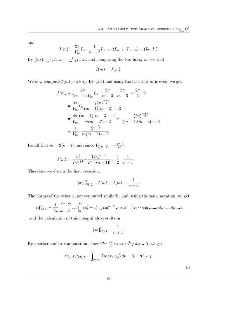
5.3. An example: the Arakelov degree of OPnOK
p1q
andJpmq � 2π
VmIm � 1
m� 2Im�1 � pIm�4 � Im�5q � � � pI2 � I1q.
By (5.8), 1m�2Im�1 � 1
m�1Im�3, and comparing the two lines, we see that
Ipmq � Jpmq.
We now compute Ipmq � Jpmq. By (5.9) and using the fact that m is even, we get
Ipmq � 2πpm� 1qVm Im �
2πm� 3
� 2πm� 5
� � � 2π3� 2
� 4πVm
Imp2πqm�4
2
pm� 1qpm� 3q � � � 3
� 4πVm
pm� 1qpm� 3q � � � 1mpm� 2q � � � 2 π � p2πqm�4
2
pm� 1qpm� 3q � � � 3
� 1Vm
� p2πqm2mpm� 2q � � � 2 .
Recall that m � 2pn� 1q, and since V2pn�1q � 2πn�1
n! ,
Ipmq � n!2πn�1
� p2πqn�1
2n�1pn� 1q! �12� 1n� 1
.
Therefore we obtain the first assertion,
}x0}2Op1q � Ipmq � Jpmq � 1n� 1
.
The norms of the other xi are computed similarly, and, using the same notation, we get
}xi}2Op1q �
1Vm
» 2π
0
» π0
. . .
» π0
�u2i � u2
i�1
�sinm�2 ϕ1 sinm�3 ϕ2 � � � sinϕm�2 dϕ1 . . . dϕm�1,
and the calculation of this integral also results in
}xi}2Op1q �1
n� 1.
By another similar computation, since @k :³π0 cosϕ sink ϕdϕ � 0, we get
xxi, xjyOp1q �»
Sm�1
Re xxi, xjy dv � 0, @i � j.
63
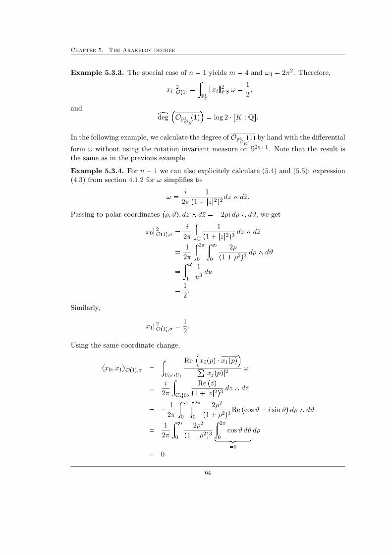
Chapter 5. The Arakelov degree
Example 5.3.3. The special case of n � 1 yields m � 4 and ω4 � 2π2. Therefore,
}xi}2Op1q �»
P1C
}xi}2FS ω �12,
and ydeg�OP1
OKp1q� log 2 � rK : Qs.
In the following example, we calculate the degree of OP1OKp1q by hand with the differential
form ω without using the rotation invariant measure on S2n�1. Note that the result isthe same as in the previous example.
Example 5.3.4. For n � 1 we can also explicitely calculate (5.4) and (5.5): expression(4.3) from section 4.1.2 for ω simplifies to
ω � i
2π1
p1� |z|2q2dz ^ dz.
Passing to polar coordinates pρ, ϑq, dz ^ dz � �2ρi dρ^ dϑ, we get
}x0}2Op1q,σ �i
2π
»C
1p1� |z|2q3 dz ^ dz
� 12π
» 2π
0
» 80
2ρp1� ρ2q3 dρ^ dϑ
�» 8
1
1u3du
� 12.
Similarly,
}x1}2Op1q,σ �12.
Using the same coordinate change,
xx0, x1yOp1q,σ �»U0XU1
Re�x0ppq � x1ppq
° |xjppq|2 ω
� i
2π
»Czt0u
Re pzqp1� |z|2q3 dz ^ dz
� � 12π
» 80
» 2π
0
2ρ2
p1� ρ2q3 Re pcosϑ� i sinϑq dρ^ dϑ
� 12π
» 80
2ρ2
p1� ρ2q3» 2π
0cosϑ dϑloooooomoooooon�0
dρ
� 0.
64

5.3. An example: the Arakelov degree of OPnOK
p1q
So,
ydeg�OP1
OKp1q
� 0� 12
¸σ
log detpxxi, xjyσq
� �12rK : Qs � log
�12
2
� log 2 � rK : Qs.
65

Chapter 5. The Arakelov degree
66

Chapter 6
The height of PnOK
Height is an important concept in diophantine geometry. It allows using descent argu-ments as used in the proof of the Mordell-Weil theorem. In this chapter, we discuss thenotion of the height of projective space as a special case of the height of an arithmeticvariety as defined by Jean-Benoıt Bost, Henri Gillet, and Christophe Soule in [BGS94].
6.1 The height of a point in PnZ
Definition 6.1.1. Let L be a Hermitian line bundle on SpecOK . Then the height ofSpecOK with respect to L is
hLpSpecOKq :�ydeg pLq.
Let X be an arithmetic variety, L a Hermitian line bundle on X, and P a point on X.Then P corresponds to a section εP : SpecOK Ñ X.
Definition 6.1.2. Let P P X be a point corresponding to the section εP : SpecOK Ñ X.We define the height of P with respect to the line bundle L as
hLpP q :�ydeg�ε�P L
�.
Consider X � PnZ and its universal bundle Op1q. In section 4.1.2 we defined the Fubini-Study metric and gave an explicit formula on Ui � tpx0 : . . . : xnq : x0 � 0u.Let P P XpCq be a point. Recall that the metric on Op1qP is the dual of the restrictionof the standard metric on Cn to the line corresponding to P . For an arbitrary section sof Op1q associated to the homogeneous polynomial
°λjXj we then get���¸λjXj
���P� |°λjzj |p° |zi|2q 1
2
.
67

Chapter 6. The height of PnOK
Example 6.1.3. Let px0, . . . , xnq be a pn� 1q-tuple of relatively prime integers and letP be the associated point in PnZ. Then,
hOp1qpP q � logb¸
x2i .
Proof. (See [Bos99], section 3.3.2.) The morphism associated to P , εP : Spec Z Ñ PnZ,corresponds to a morphism of graded rings,
ε#P : ZrX0, . . . , Xns ÝÑ ZrY s
Xi ÞÝÑ xiY.
Furthermore, we have a canonical isomorphism of line bundles ε�POPnp1q � OSpec Zassociating ε�PXi to xi. Under this map, a global section s � °λjXj is sent to
°λjxj .
By scaling of the λj (the section is independent of the scaling) we get°λjxj � �1.
Therefore the norm at infinity of ε�P s is���¸λjXj
���P� |°λjxj |b°
x2i
� 1b°x2i
.
Now the product formula and the definition of the Arakelov degree complete the proof.
Remark 6.1.4. For an arbitrary point P � px0 : . . . : xnq P PnpKq, the height definedabove coincides with the classical height in Arakelov theory (definition A.3.6)
hpP q �¸p-8
logpmaxi|xi|pq �
¸σ:KãÑC
log
�¸i
|σpxiq|2� 1
2
,
where p runs over the prime ideals of OK and | � |p is the absolute value correspondingto the non-archimedean valuation vp. (See [BGS94], p. 947.)
In the case K � Q, this coincides with our result in the lemma above because Z is aprincipal ideal domain and therefore the finite primes do not contribute to the sum.
Example 6.1.5. Consider the point p0 : 1q P P1OK :
hpp0 : 1qq � log 1 � 0.
6.2 The height of PnOK
In this section, for simpler notation, we often omit the index PnOK and simply write Op1qfor OPnOK
p1q as in section 5.3
68

6.2. The height of PnOK
Definition 6.2.1. The height of PnOK with respect to OPnOKp1q with the metric induced
by the Fubini-Study metric is
hOp1qpPnOK q � hOp1q|div spdiv sq �
»pPnOK qpCq
log }s}ωn, (6.1)
where s is a non-zero section of OPnOKp1q and ω is the differential form associated to the
Fubini-Study metric (section 4.1.2).
Remark 6.2.2. For s � x0, OPnOKp1q|div s � OPn�1
OKp1q
Lemma 6.2.3. In the above notation,
hOp1qpP1OK q �
12� rK : Cs.
Proof. We choose the section s � x0.
1. The divisor div x0 � p0 : 1q, and by example 6.1.5, hOp1qpdiv x0q � 0.
2. We now need to compute the integral in formula (6.1). Recall that
P1OK pCq �
§σ:KãÑC
pP1OK qσpCq,
and that for each σ the computation is similar. Thus,
hpP1OK q � �rK : Qs �
»P1
C
log }s}ω, (6.2)
where ω is the differential form (4.3) from section 4.1.2.
This integral can be taken over the standard open set U0 � tpx0 : x1q : x0 � 0u �C. By setting z � x1
x0,
�»
P1C
log }s}ω � �»
Clogpp1� |z|2q� 1
2 q�i
2π1
p1� |z|2q2dz ^ dz
� i
2π
»C
logp1� |z|2q2p1� |z|2q2 dz ^ dz.
Passing to polar coordinates pρ, ϑq and dz ^ dz � �2ρi dρ^ dϑ,
� � i
2π
» 2π
0
» 80
logp1� ρ2q2p1� ρ2q2 2ρi dρ^ dϑ,
69

Chapter 6. The height of PnOK
and changing the coordinates to µ � ρ2, we obtain 2ρ dρ^ dϑ � dµ^ dϑ and
� 12π
» 2π
0
» 80
logp1� µq2p1� µq2 dµ^ dϑ
�» 8
0
logp1� µq2p1� µq2 dµ
��� logp1� µq
2p1� µq � 12p1� µq
����80
� 12.
So,
hOp1qpP1OK q � rK : Qs � 1
2.
Theorem 6.2.4. (Bost, Gillet, Soule, [BGS94]) The height of PnOK is
hOp1qpPnOK q � rK : Qs � σn,
where σn is the Stoll number, i.e. σn � 12
n
k�1
k
l�1
1l
.
Proof. Choose the section s � x0. Then, div s � Pn�1OK .
Let dv be the unique Upn � 1q-invariant probability measure on the unit sphere S2n�1
in Cn�1. Then, by [BGS94], p. 924,»PnC
log }x0}ωn �»
S2n�1
log |x0| dv.
One can compute the integral on the right-hand side as in section 5.3 to be»S2n�1
log |x0| dv � �12
�n
l�1
1l
�.
By definition 6.2.1,
hpPnOK q � hpPn�1OK q � rK : Qs
»S2n�1
log |x0| dv
� hpPn�1OK q � rK : Qs 1
2
�n
l�1
1l
�. (6.3)
70

6.3. Arakelov degree and height – intersection theory
The desired result is obtained by induction on n:In example 6.1.5, we explicitly computed the base case, namely for n � 1,
div x0 � p0 : 1q P P1.
The induction step follows from equation (6.3).
6.3 Arakelov degree and height – intersection theory
In the light of the historic development of Arakelov Theory, we now discuss the resultof theorem 6.2.4 above in detail.
Intersection theory is a branch of algebraic geometry, which studies linear combinationsof subvarieties of algebraic varieties and their intersections. Their intersections, on theone hand, are motivated by the set-theoretic intersection, but on the other hand, this isextended such that one can e.g. compute the intersection product of two lines. We willnot discuss intersection theory here, as this would go beyond the scope of this thesis,but we will touch it now and then (see e.g. remark 8.1.7 and section 10.4).
In the paper that led to the theory named after him, [Ara74], Arakelov introduced anintersection theory on arithmetic surfaces and thus extended the theory on varietiesover fields to a theory on arithmetic surfaces. Gerd Faltings, in his seminal paper[Fal84], pushed this theory further and proved a Riemann-Roch theorem, a Hodge indextheorem, and a Noether’s formula for arithmetic surfaces. Moreover, this eventually ledhim to his proof of the Mordell conjecture (now called Faltings’ theorem), the Shafarevichconjecture, and a conjecture of Tate.
Henri Gillet and Christophe Soule later generalized this to a product on arithmeticvarieties in a series of papers, among them [GS90], and proved a version of the Riemann-Roch theorem in this context in [GS89] and [GS92].
In the context of this arithmetic intersection product on arithmetic varieties, the heightof an arithmetic variety with respect to a Hermitian vector bundle was defined to be thedegree of a certain intersection product in [BGS94], and therefore the height is a specialcase of the degree.
In fact, for PnOK respectivelyOPnOKp1q, the degree and the height should actually coincide.
Now, our results in theorem 5.3.1 and theorem 6.2.4 are not the same, and we will nowelaborate on what leads to this difference.
In [BGS94], Proposition 3.3.2, it is shown that, when changing the metric, the heightessentially only changes up to a constant. We furthermore observe that, indeed, ourresults are asymptotically equivalent as n tends to infinity:
Recall that
ydeg OPnOKp1q � rK : Qs
2� pn� 1q logpn� 1q,
71
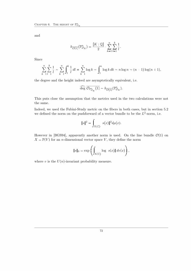
Chapter 6. The height of PnOK
and
hOp1qpPnOK q �rK : Qs
2�n
k�1
k
l�1
1l.
Since
n
k�1
k
l�1
1l�
n
k�1
» k1
1ldl �
n
k�1
log k �» n
1log k dk � n log n � pn� 1q logpn� 1q,
the degree and the height indeed are asymptotically equivalent, i.e.
ydeg OPnOKp1q � hOp1qpPnOK q.
This puts close the assumption that the metrics used in the two calculations were notthe same.
Indeed, we used the Fubini-Study metric on the fibers in both cases, but in section 5.2we defined the norm on the pushforward of a vector bundle to be the L2-norm, i.e.
}s}2 �»XpCq
}spxq}2dµpxq.
However in [BGS94], apparently another norm is used. On the line bundle Op1q onX � PpV q for an n-dimensional vector space V , they define the norm
}s}0 � exp
�»XpCq
log }spxq} dvpxq�,
where v is the Upnq-invariant probability measure.
72

Chapter 7
The canonical polygon
Canonical polygons form a tool to bridge between Arakelov theory and geometry ofnumbers. We first give the definition and, as a continuation of the example in section5.3, we consider the canonical polygon for the twisting sheaf. We then look at successiveminima and discuss morphisms between vector bundles.
In this chapter, if we do not state otherwise, we always use the induced metric onsubbundles of a given Hermitian vector bundle E.
7.1 Definition
Definition 7.1.1. The normalized Arakelov degree is
xdeg E � 1rK : Qs
ydeg E,
and the normalized slope is pµpEq � 1rkE
xdeg E.
Remark 7.1.2. It is sometimes more natural to consider the normalized Arakelov degreeor the normalized slope instead of the Arakelov degree since they are invariant underthe pullback under the morphism f associated to an extension of number fields [Bos96].In the literature, the normalized Arakelov degree often is denoted by ydeg npEq.
Definition 7.1.3. Let E be a Hermitian vector bundle over SpecOK . Consider the setof points tprk F , xdeg F q, F is a subbundle of Eu � r0, rk Es � R. The convex hull of thisset is bounded from above ([Bos96], A.3). Its upper boundary defines a piecewise linearfunction PE : r0, rkEs Ñ R, which is called the canonical polygon. If PE is linear, wesay that E is semi-stable.
73

Chapter 7. The canonical polygon
Furthermore, for each i P t1, . . . , rk Eu, we define the i-th slope of E to be
pµipEq � PEpiq � PEpi� 1q,
so pµipEq is the slope of PE in the interval pi� 1, iq.The maximal and minimal slopes are denoted by pµmaxpEq, pµminpEq, respectively.
Remark 7.1.4. Note that PEp0q � 0, PEprk Eq � xdegpEq, and°i pµipEq � xdegpEq.
Moreover, since PE is a concave function,
@i P t1, . . . , rk Eu : pµi�1pEq ¥ pµipEq.In particular,
pµmaxpEq � pµ1pEqpµminpEq � pµrkEpEq.
Example 7.1.5. We want to calculate the canonical polygon of E � pπ�OP1Zp1q, hFSq,
where hFS is the metric induced by the Fubini-Study metric.
Recall that ΓpSpec Z, π�OP1Zp1qq � ΓpP1
Z,OP1Zp1qq � Zx0 � Zx1. In example 5.3.4 we
calculated}x0}2OP1
Z� }x1}2OP1
Z� 1
2,
xx0, x1yOP1Z� 0,
and ydegOP1Zp1q � log 2.
Since rQ : Qs � 1, xdegE �ydeg E; so PEp2q � log 2.
Subbundles of π�OP1Zp1q correspond to submodules of Zx0 � Zx1. We now consider the
submodules of rank 1:All submodules of Zx0�Zx1 of rank 1 are of the form N � Zpax0� bx1q, where a, b P Z,not both 0. We calculate the degree using the section s � ax0 � bx1 in definition 5.1.1.
1. Clearly, log #pZpax0 � bx1q{Zpax0 � bx1qq � 0.
2. Since xx0, x1yOP1Z� 0,
}ax0 � bx1}2 � |a|2}x0}2 � |b|2}x1}2 � 12p|a|2 � |b|2q.
Therefore,
ydeg pZpax0 � bx1qq � �12
log�
12p|a|2 � |b|2q
� 1
2log 2� 1
2log�
1|a|2 � |b|2
.
74

7.2. Slopes and successive minima
Since a, b P Z, log�
1|a|2�|b|2
¤ 0, and so
xdegpZpax0 � bx1qq �ydeg pZpax0 � bx1qq � 12
log 2� 12
log�
1|a|2 � |b|2
¤ 1
2log 2.
This bound is attained at e.g. a � 1, b � 0: xdegpZx0q � 12 log 2.
The point p1, 12 log 2q already lies on the line between p0, PEp0qq � p0, 0q and p2, PEp2qq �
p2, log 2q, so taking the convex hull does not change the upper boundary of the settprk F ,ydeg F q, F is a subbundle of Eu. So PEp1q � 1
2 log 2.
In particular, pµ1pEq � pµ2pEq � 12 log 2, so PE is linear. Thus, π�OP1
Zp1q is semi-stable.
y
x
p1, PEp1qq
p2, PEp2qq
0 1 2
12 log 2
log 2
7.2 Slopes and successive minima
We start this section by looking at an example.
Example 7.2.1. Consider the lattice Λ � Z � pa, bq �Z � pc, dq � R2, where a, b, c, d P R.Λ is a Z-module and we endow Λ bZ C � C2 with the standard Hermitian metric. Wecompute the degree of Λ and the degree of a given submodule.
Let e1 � pa, bq and e2 � pc, dq. Clearly,
}e1}2 � a2 � b2, }e2}2 � c2 � d2 and xe1, e2y � ac� bd.
We compute the determinant detpei, ejq:
detpxei, ejyq � pa2 � b2qpc2 � d2q � pac� bdq2 � pad� bcq2 � pdetpei, ejqq2.
So the Arakelov degree of Λ is
xdegΛ � � log pVolpPqq ,
where P is the fundamental parallelogram of the lattice Λ.
75

Chapter 7. The canonical polygon
y
x
e2e1
P
Let Λ1 be a sublattice of Λ. Then, Λ1 � pαe1 � βe2qZ for some α, β P Z, and
xdegppαe1 � βe2qZq � � log }αe1 � βe2}.
So maximizing the degree of a submodule of Λ is equivalent to finding a shortest vectorin the lattice Λ. This leeds to the problem of successive minima.
Definition 7.2.2. Let C be a convex body which is symmetric with respect to theorigin and Λ a lattice in Rn. The successive minima λi � λipC,Lq, i � 1, . . . n, of Cwith respect to Λ are defined by
λi � mintλ ¡ 0 : λC contains i linearly independent points of Lu.See [Gru07] for more on successive minima.
In the example above, we considered a Hermitian vector bundle E over Spec Z, i.e. aZ-module E endowed with a metric } � }. We take C � Bn, where Bn is the closedunit ball in Rn endowed with the standard metric, and, since we were dealing with aZ-module, we get the following equality:
Let λ � Ze1 � � � � � Zen � Rn. Then
pµ1 � PΛp1q � suprkN�1
xdegN
� suppa1,...,anqPZn
t� log }a1e1 � � � � anen}u
� � log minpa1,...,anqPZn
t}a1e1 � � � � anen}u
� � log λ1.
For arbitrary K, we just get an inequality:
76

7.2. Slopes and successive minima
Lemma 7.2.3. Let E be a Hermitian vector bundle on SpecOK , i.e. an OK-moduleendowed with a Hermitian metric. Then
log λ1pEq ¥ �pµ1pEq.
Proof. See [Bor05]. Let s P E be an element such that maxσ:KãÑC }s}σ � λ1pEq. Then,using the section s of sOK ,
ydeg psOKq � log #psOK{sOKqloooooooooomoooooooooon�0
�¸
σ:KãÑClog }s}σ ¥ � log λ1pEq � rK : Qs.
Since sOK is a subbundle of E, we get the desired result by the definition of pµ1pEq.
One can show even more: in fact, the inequality holds for all i.
Proposition 7.2.4. (Borek, [Bor05]) Let E be a Hermitian vector bundle on SpecOK .Then,
@i : log λipEq ¥ �pµipEq.Example 7.2.5. We take pa, bq � p2, 0q and pc, dq � p3, 4q in the previous example.Then xdegΛ � logpdet
�2 30 4
q � log
18� 3 log 12.
The shortest vector in the lattice is p2, 0q, and the degree of the generated sublattice is
xdegpp2, 0q � Zq � log12.
So we get
PΛp1q � log12, PΛp2q � 3 log
12.
Note that Λ is not semi-stable.
y
x
p1, PΛp1qq
p2, PΛp2qq
0 1 2
3 � log 12
log 12
77
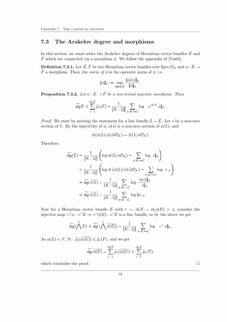
Chapter 7. The canonical polygon
7.3 The Arakelov degree and morphisms
In this section, we want relate the Arakelov degrees of Hermitian vector bundles E andF which are connected via a morphism φ. We follow the appendix of [Via05].
Definition 7.3.1. Let E, F be two Hermitian vector bundles over SpecOK and φ : E ÑF a morphism. Then, the norm of φ is the operator norm of φ, i.e.
}φ}σ :� sup0�sPE
}φpsq}σ}s}σ .
Proposition 7.3.2. Let φ : E Ñ F be a non-trivial injective morphism. Then
xdegE ¤rk E
i�1
pµipF q � 1rK : Qs
¸σ:KãÑC
log } ^rkE φ}σ.
Proof. We start by proving the statement for a line bundle L � E. Let s be a non-zerosection of L. By the injectivity of φ, φpsq is a non-zero section of φpLq, and
#pφpLq{φpsqOKq � #pL{sOKq.Therefore,
xdegpLq � 1rK : Qs
�log #pL{sOKq �
¸σ:KãÑC
log }s}σ�
� 1rK : Qs
�log # pφpLq{φpsqOKq �
¸σ:KãÑC
log }s}σ�
� xdeg φpLq � 1rK : Qs
¸σ:KãÑC
log}φpsq}σ}s}σ
¤ xdeg φpLq � 1rK : Qs
¸σ:KãÑC
log }φ}σ.
Now for a Hermitian vector bundle E with r :� rkE � rkφpEq ¡ 1, consider theinjective map ^rφ : ^rE Ñ ^rφpEq. ^rE is a line bundle, so by the above we get
xdegpr©Eq ¤ xdeg p
r©φpEqq � 1
rK : Qs¸
σ:KãÑClog } ^r φ}σ.
As φpEq � F , @i : pµipφpEqq ¤ pµipF q, and we get
xdeg φpEq �rk E
i�1
pµipφpEqq ¤ rk E
i�1
pµipF q,which concludes the proof.
78

7.3. The Arakelov degree and morphisms
Corollary 7.3.3. Under the assumptions above,
xdegE ¤rk E
i�1
pµipF q � rkErK : Qs
¸σ:KãÑC
log }φ}σ.
Proof. By e.g. [Bos99], } ^r φ} ¤ }φ}r.Proposition 7.3.4. Let φ : E Ñ F be a non-trivial injective morphism. Then
pµmaxpEq ¤ pµmaxpF q � 1rK : Qs
¸σ:KãÑC
log }φ}σ.
Proof. Let pr, PEprqq be the point of discontinuity of PE such that r ¡ 0 is minimal.Let Er be a submodule of E of rank r such that PEpErq � xdeg Er � r � pµmaxpEq. Byapplying corollary 7.3.3 to the morphism φ|Er : Er Ñ φpErq,
pµmaxpEq �xdeg Err
¤ 1r��
r
i�1
pµipφpErqq � r
rK : Qs¸
σ:KãÑClog }φ|Er}σ
�,
and since pµipφpErqq ¤ pµmaxpφpErqq ¤ pµmaxpF q and }φ|Er}σ ¤ }φ}σ, we get the desiredresult.
79
Chapter 7. The canonical polygon
80

Chapter 8
Chow groups
In this chapter, we give an outlook on an alternative, more geometric, interpretationof isomorphism classes of Hermitian vector bundles as used e.g. in [BGS94]. We startby considering the classical case of algebraic cycles on algebraic varieties over a field k,e.g. a number field. Then, to bring in arithmetic, we extend this notion to arithmeticvarieties, i.e. varieties over the ring of integers of a number field with some additionalproperties. In 8.2, we introduce arithmetic cycles and Chow groups. We then sketch theproof showing that the first arithmetic Chow group and the arithmetic Picard group areisomorphic and thus, this approach indeed represents a new interpretation.
We will be brief on technical details, as the intention of this section is to give an in-troduction to this setting. However, the technicalities can be found in [Ful98], [Sou92],[BGS94], and [Lan88].
8.1 Geometric Chow groups
Chow rings are a geometric analogon of cohomology rings of a variety in topology. Theyare a generalization of the divisor class group, which has a long history in the study ofalgebraic geometry. The notion of rational equivalence was first introduced by Severi.For an overview of the historic development of Chow rings, see [Ful98].
Definition 8.1.1. Let X be an algebraic scheme. An algebraic cycle on X is a for-mal linear combination of irreducible closed subvarieties on X with integer coefficients,i.e. element of the group
ZpXq � àV�X
Z � V,
where V runs over the irreducible closed subvarieties of X. An algebraic cycle of dimen-sion p or p-cycle on X is an algebraic cycle on X such that all subvarieties of X whichhave non-zero coefficient have dimension p. The group of algebraic cycles of dimensionp is denoted by ZppXq.
81
Chapter 8. Chow groups
A cycle Z � °ni � Vi is called positive if it is not zero and each of its coefficients ni is anon-negative integer.
Remark 8.1.2. The divisors of X are the algebraic cycles of codimension 1, i.e.
DivpXq � ZdimX�1pXq.
We introduce the order of vanishing of r along V for a subvariety V of X of codimensionone to define the cycle associated to a rational function. The construction is similar tothat of principal divisors in definition 3.5.4.
Let X be a variety which is non-singular in codimension one and V a subvariety of X ofcodimension one. Then the local ring of X along Y, OX,V , is a discrete valuation domain.Furthermore, kpXq � QuotOX,V . Let r P kpXq� be a nonzero rational function on X.This can be written as r � a{b, where a, b P OX,V .
Definition 8.1.3. The order of vanishing of r along V is defined to be
ordV prq � ordV paq � ordV pbq,where the orders on the right are those with respect to the valuation of the discretevaluation ring OX,V .
Remark 8.1.4. In case that X possibly is singular, one can define
ordV prq � lOX,Y pOX,Y {prqq,where lOX,Y denotes the length of the OX,Y -module OX,Y {prq.Definition 8.1.5. For any p � 1-dimensional subvariety W of X, and any r P kpW q�,i.e. a non-zero rational function on W , let div r be the p-cycle
div r �¸
ordV prq � V,where the sum is taken over all subvarieties of codimension one of W . A p-cycle Z iscalled rationally equivalent to zero if there exist p� 1-dimensional subvarieties Wi of Xand ri P kpWiq� such that
Z �¸
div ri.
Note that the set of p-cycles rationally equivalent to zero form a subgroup of ZppXqsince div r�1 � �div r, denoted by RppXq.Definition 8.1.6. The group of p-cycles modulo rational equivalence is called the (ge-ometric) Chow group of dimension p,
CHppXq � ZppXq{RppXq.The (geometric) Chow group is the direct sum
CHpXq �dimXàp�0
CHppXq.
82

8.2. Arithmetic Chow groups
Remark 8.1.7. One can equip CHpXq with a product to make it into a ring, the Chowring. This product is called the intersection product. In section 6.3, we briefly mentionedintersection theory and its generalization to arithmetic varieties. Even though it will bementioned several times in this thesis, we will not go into the details of intersectiontheory, as this would be beyond the scope. For a thorough reference on intersectiontheory, see [Ful98].
8.2 Arithmetic Chow groups
Throughout this section, let X be an arithmetic variety and X be a smooth projectivecomplex equidimensional variety of dimension d.
To define the arithmetic counterpart of algebraic cycles, we first need some terminologyof complex geometry. In particular, we need the notions of Green currents on smoothprojective complex varieties.
Notation. Let X be a smooth projective complex equidimensional variety of dimensiond. We denote by Ap,qpX q the vector space of complex valued differential forms of typepp, qq. A current δ is a smooth linear functional on Ap,qpX q, i.e. a differential form withdistribution coefficients. We denote by Dp,qpX q the set of all currents. Note that there isan inclusion Ap,qpX q ãÑ Dp,qpX q given by ω ÞÑ �
α ÞÑ ³X ω ^ α
�. We remark that, more
generally, just like in the theory of distributions, any locally L1 form of type pp, qq on Xdefines a current on X (see [Sou92], p. 39, chapter II.1 and [BGS94], p. 908 for details).
For any irreducible analytic subvariety Y of X , we can define a current δY by setting
δYpαq :�»Yns
i�α @α P Ad�p,d�q,
where i : Y ãÑ X and Yns is the smooth part of Y. We extend this definition by linearityto any analytic cycle of X .
Definition 8.2.1. A Green current for an analytic cycle Z of codimension p on X isan element g P Dp�1,p�1pX q such that
ddcg � δZ P ApppX q,where d � B � B and dc � i
4π pB � Bq.
Now we can define the arithmetic analogs. For an arithmetic variety X, we denote byApppXRq the vector space of real differential forms in ApppXpCqq and by DpppXq the setof real currents in DpppXpCqq. We can associate a current δZ to a cycle Z � °i niZi bysetting δZ �
°i niδZipCq.
Definition 8.2.2. A Green current for a cycle Z of codimension p on X is a currentg P Dp�1,p�1pXRq such that ddcg � δZ is smooth, i.e. a Green current for ZpCq whichlies in Dp�1,p�1pXRq.
83

Chapter 8. Chow groups
Definition 8.2.3. An arithmetic cycle of dimension p on X is a pair pZ, gZq, where Zis a cycle of codimension p and gZ is a Green current for Z. Let pZppXq be the group ofarithmetic cycles of dimension p, where addition is defined componentwise.
Giving examples for arithmetic cycles is not easy, and we only sketch the idea of anexample for an arithmetic cycle. For this, we need the following theorem, the Poincare-Lelong formula. For more details on this example and a proof of the theorem, see [Sou92],p. 41, Theorem II.2 and p. 54ff, Chapter III.
Theorem 8.2.4. (The Poincare-Lelong formula) Let L � pL, } �}q be a holomorphic linebundle on X and s a meromorphic section of L. Then � log }s}2 P L1pX q and henceinduces a distribution in D00pX q which furthermore is a Green current for div psq.Example 8.2.5. Let y be a point on an arithmetic variety X such that Y � tyuis a closed integral subscheme of X of codimension p � 1. Let f P kpyq�. Thenpdiv pfq,�rlog |f |2sq is an arithmetic cycle on X, where rlog |f |2s is a certain Greencurrent on X associated to log |f |2.
Definition 8.2.6. We denote by pRppXq � pZppXq the subgroup generated by the pairspdiv f,�rlog |f |2sq from the example above and by pairs p0, Bpuq � Bpvqq, where u and vare currents of type pp� 2, p� 1q and pp� 1, p� 2q, respectively.Then the arithmetic Chow group of codimension p of X is defined as the quotient
yCHppXq :� pZppXq{ pRppXq.Remark 8.2.7. Arithmetic Chow groups clearly are a generalization of geometric Chowgroups in classical algebraic geometry as defined in the previous section. To the classical,“geometric”, part, an additional, “analytic”, part is added.
We now come to the main proposition of this section, namely we discuss the correspon-dence between the first arithmetic Chow group and the arithmetic Picard group of anarithmetic variety.
Proposition 8.2.8. Using the notation of the example above, there is an isomorphism
pc1 : xPicpXq ÝÑ yCH1pXq,
mapping the class of pL, } � }q to the class of pdiv s,�rlog }s}2sq for any rational sections of L.
Sketch of proof. We first show the well-definedness of this map. Since L is a line bundle,the set of global sections of L has rank 1. Therefore, any other rational section of L can bewritten as s1 � fs, where f is a rational function on X. So, div s1 � div s. Furthermore,a calculation similar to the one in (4.2) in section 4.1.2 shows that pc1pL, } � }q does notdepend on the choice of the section.
84

8.2. Arithmetic Chow groups
We consider the inverse map. This is given by sending a cycle pZ, gZq to the isomorphismclass of pOXpZq, } � }q, where the metric is locally given by }f}2 � |f |2e�gZ . Since gZis a Green current for Z, this defines a smooth metric and hence this defines a smoothmetric.
Remark 8.2.9. pc1pL, } � }q is called the first (arithmetic) Chern class of pL, } � }q. Theconcept of Chern classes comes from classical differential geometry and is a topologicalinvariant of Hermitian vector bundles; e.g. given a Hermitian line bundle pL, } � }q, theassociated first Chern form is the differential form given by pc1pL, }�}q � �ddc log }spzq}2.Note that in section 4.1.2, we calculated the first Chern form of the Fubini-Study metricon Op1q. The Chern class then is the class of the first Chern form in the second deRham cohomology group, [GH78, Lan88, Deb05].
85

Chapter 8. Chow groups
86
Chapter 9
Arithmetic surfaces and thedegree of an elliptic curve
In this chapter, we introduce the notions needed to apply Arakelov theory to ellipticcurves. We show how to attach a scheme over Z – or, more precisely, an arithmetic surface– to an elliptic curve. We define theta functions and examine how they correspond toglobal sections of line bundles on complex tori, i.e. elliptic curves. Using theta functions,we define a norm on the line sheaf OpP q for P � OE . Finally, we state a result of JurgKramer on the Arakelov degree of a special line bundle on an elliptic curve.
9.1 Arithmetic surface attached to an elliptic curve
Definition 9.1.1. Let R be a Dedekind domain and K its field of fractions. Then, anarithmetic surface over R is a scheme C over R whose generic fiber is a non-singularconnected projective curve C{K and whose special fibers are unions of curves over theappropriate residue fields. Furthermore, we require some technical conditions: C isintegral, normal, excellent, and is flat and of finite type over R.
Remark 9.1.2. One can consider an arithmetic surface as a curve over SpecR since therelative dimension is one, i.e. the fibers are one-dimensional. Note that the fibers arenot necessarily regular, they can also be reducible. Nevertheless, an arithmetic surfaceis regular in codimension one and therefore has a theory of Weil divisors. See [Sil94] fordetails.
Now let C � P2Z be the Z-scheme defined by the equation
Y 2 � X3 � aX � b,
where a, b P Z and ∆ � �16p4a3 � 27b2q � 0. Then the generic fiber of C is the ellipticcurve over Q defined by the equation above.
87

Chapter 9. Arithmetic surfaces and the degree of an elliptic curve
The fibers over closed points p are given by prime ideals, and the fiber then is
Cp � C �Z p,
the reduction modulo p.
If p � pZ, for a prime p P Z, then Cp is exactly what “reduction mod p” should be,namely the scheme over Z{p � Fp given by Y 2 � X3 � aX � b, where a � a mod p andb � b mod p.
Furthermore, the scheme C is proper over Z, since C is a closed subscheme of projectivespace over Spec Z ([Sil94], Theorem IV.2.8.). This is a rather technical condition, butwe need it below to extend rational points on the elliptic curve which is the generic fiberof an arithmetic surface.
Example 9.1.3. Consider the elliptic curve Y 2 � X3 � 3X � 6 over Z. The fibers overprimes p are given by reduction modulo p, i.e. by the equation Y 2 � X3 � 3X � 6 overFp, where 3 � 3 mod p, and 6 � 6 mod p. The discriminant is ∆ � �27 � 33 � 5, sofor every prime p � 2, 3, 5, Cppq is an elliptic curve over Fp; in particular, the fiber isnon-singular.
• For p � 2, we get the curve Cp2q : Y 2 � XpX � 1q2, which has a double point,
• for p � 3, we get Cp3q : Y 2 � X3, which has a cusp,
• and for p � 5 we get Cp5q : Y 2 � pX � 1qpX � 2q2, which also has a double point.
We can illustrate this in the following figure:
p0q p2q p3q . . . ppq . . . pqq . . .
π
Spec Z
C
Cp0q Cp2q Cp3q Cppq Cpqq
The fibers over p2q, p3q, and p5q are singular. The generic fiber is the fiber over p0q. Thefibers over other primes ppq, pqq are regular. See [Sil94], p.300, Examples IV.2.2.1-2.2.3and p. 311ff for more details and similar examples.
88

9.1. Arithmetic surface attached to an elliptic curve
As stated in the remark above, there is a theory of Weil divisors on arithmetic surfaces.In fact, irreducible divisors only have two possible forms: horizontal or fibral divisors.For this, we need the following result of algebraic geometry.
Proposition 9.1.4. Let φ : C1 Ñ C2 be a morphism of curves. Then φ is either constantor surjective.
Proof. [Sil86], p. 24, Theorem II.2.3 or [Har77], Proposition II.6.8.
Proposition 9.1.5. Every irreducible divisor on an arithmetic surface C {R is either
1. contained in a special fiber (fibral divisor) or,
2. maps surjectively onto SpecR (horizontal divisor).
Proof. If D is an irreducible divisor which is not contained in a special fiber, consider theprojection map π : D Ñ SpecR induced by the projection map of the scheme C . Thisis not constant, since D does not lie in a special fiber, so, by the previous proposition,it is surjective.
We now consider rational points on the generic fiber of an arithmetic surface. If R is aring, recall definition 2.2.11 of R-valued points of an R-scheme X:
If R is a ring and X an R-scheme, the set of R-valued points of X is the set
XpRq � tR-morphisms SpecRÑ Xu.Remark 9.1.6. Note that one can identify the image of a section σ : SpecRÑ C witha horizontal divisor on C .
We can identify rational points on the generic fiber of an arithmetic surface, i.e. pointsin CpKq, with R-valued points of C :
Theorem 9.1.7. ([Sil94], Corollary IV.4.4 (a)) Let R be a Dedekind domain and K itsfield of fractions, let C {R be an arithmetic surface and C{K its generic fiber. If C isproper over R,
CpKq � C pRq.
This theorem tells us that rational points on an elliptic curve “extend” to a section ofthe associated arithmetic surface, i.e. define a horizontal divisor on C .
The following theorem/definition is a bit technical, but we need the result for the examplein the next section. The first assertion was proven by Abhyankar and Lipman, the secondis due to Lichtenbaum and Shafarevich.
Theorem 9.1.8. ([Sil94] p. 317, Theorem IV.4.5) Let R be a Dedekind domain and Kits field of fractions, and let C{K be a non-singular projective curve of genus g. Then
89

Chapter 9. Arithmetic surfaces and the degree of an elliptic curve
1. (Resolution of Singularities for Arithmetic Surfaces) There exists a regular arith-metic surface C {R, proper over R, whose generic fiber is isomorphic to C{K. Wecall C {R a proper regular model for C{K.
2. (Minimal Models Theorem) Assume that g ¥ 1. Then there exists a proper regularmodel C min{R for C{K with the following minimality property:
Let C {R be another proper regular model for C{K. Fix an isomorphism from thegeneric fiber of C to the generic fiber of C min. This induces an R-birational mapC Ñ C min, which is an R-isomophism. C min is called the minimal proper modelfor C{K. It is unique up to isomorphism.
9.2 Theta functions
Theta functions play an important role in the theory of elliptic curves, or – more generally– in the theory of Abelian varieties. They are related to the Weierstrass ℘-function (see[Sha94a], p. 145, 152) and give a projective embedding of tori C{Λτ , where Λτ � Z� τZ(Lefschitz Theorem, see e.g. [Mur93], p. 51).
Remark 9.2.1. For higher dimensional tori, they do not aways give such an embedding.In this case, this holds if there is a positive line bundle on the torus, i.e. a line bundlewith positive first Chern class, see e.g. [Mur93]. This is a special case of the Kodairatheorem [GH78], p. 181, which gives a projective embedding for a compact complexmanifold with a positive line bundle.
9.2.1 Jacobi theta functions
Definition 9.2.2. Let H denote the complex upper half plane, i.e.
H � tτ P C : Im τ ¡ 0u.
Definition 9.2.3. The standard theta function on C�H is defined as
ϑpz, τq �¸mPZ
eπim2τ�2πimz.
Proposition 9.2.4. For every k P Z, the theta function satisfies the following:
1. ϑpz � k, τq � ϑpz, τq and
2. ϑpz � kτ, τq � ϑpz, τqe�πik2τ�2πikz.
Proof. The first assertion is clear since e2πik � 1 for k P Z.
90
9.2. Theta functions
Since
ϑpz � kτ, τq �¸mPZ
eπim2τ�2πimpz�kτq
�¸mPZ
eπipm�kq2τ�2πipm�kqz � e�πik2τ�2πikz
� ϑpz, τqe�πik2τ�2πikz,
the second property follows.
Often it is useful to also consider the related theta functions with characteristics:
Definition 9.2.5. The theta functions with characteristics pα, βq are given on C�H by
ϑα,βpz, τq �¸mPZ
eπipm�αq2τ�2πipm�αqpz�βq,
for α, β P C. If l P Z such that α, β P 1lZ, we say that ϑα,β has level l. A special case
are the Jacobi theta functions, which have level 2. They are usually written as
ϑ00pz, τq � ϑ0,0pz, τqϑ01pz, τq � ϑ0, 1
2pz, τq
ϑ10pz, τq � ϑ 12,0pz, τq
ϑ11pz, τq � ϑ 12, 12pz, τq.
Remark 9.2.6. Note that ϑα,βpz, τq � ϑpz � ατ � β, τqeπiα2τ�2πiαpz�βq, in particular,ϑ0,0pz, τq � ϑ00pz, τq � ϑpz, τq. Often one uses the more general Riemann theta function,which is defined on Cn�Hn, where Hn is the Siegel upper half space. Even, more general,one defines a theta function by means of a functional equation, as we will see later.
We use [Mur93] for the following propositions.
Proposition 9.2.7. Let l P Z, l ¥ 2, and let α, β P 1lZ. The theta functions with
characteristics pα, βq satisfy
1. ϑα,βpz � l, τq � ϑα,βpz, τq and
2. ϑα,βpz � lτ, τq � ϑα,βpz, τqe�πil2τ�2πilz.
Proof. Both properties follow from proposition 9.2.4 and remark 9.2.6:
ϑα,βpz � l, τq � ϑpz � l � ατ � β, τqeπiα2τ�2πiαpz�l�βq
� ϑpz � ατ � β, τqeπiα2τ�2πiαpz�βq � e2πiαl
� ϑα,βpz, τqe2πiαl
� ϑα,βpz, τq,
91

Chapter 9. Arithmetic surfaces and the degree of an elliptic curve
since α � l P Z. The second property is shown similary:
ϑα,βpz � lτ, τq � ϑpz � lτ � ατ � b, τqeπiα2τ�2πiαpz�lτ�βq
� ϑpz � ατ � β, τqe�πil2τ�2πilpz�ατ�βq � eπiα2τ�2πiαpz�lτ�βq
� ϑpz � ατ � β, τqeπiα2τ�2πiαpz�βq � e�πil2τ�2πilpz�βq
� ϑα,βpz, τqe�πil2τ�2πilz,
since β � l P Z.
Proposition 9.2.8. The Jacobi theta functions satisfy the following properties for everyk P Z:
1. ϑijpz � k, τq �#
ϑijpz, τq if i � 0�ϑijpz, τq if i � 1,
and
2. ϑijpz � kτ, τq �#
ϑijpz, τqe�πik2τ�2πikz if j � 0�ϑijpz, τqe�πik2τ�2πikz if j � 1.
Proof. The proof is analogous to the one above.
Theorem 9.2.9. Let τ P H be fixed, and, for simpler notation, denote ϑα,βpz, τq simplyby ϑα,βpzq. Then the holomorphic map ϕ : C{Λτ Ñ P2
C defined by
ϕpzq � pϑ0,0pzqϑ1,1pzq2 : ϑ1,0pzqϑ0,1pzqϑ1,1pzq : ϑ0,0pzq3qinduces an isomorphism from C{Λτ onto the smooth cubic with homogeneous equation
Y 2Z � XpαX � βZqpβX � αZq,
where α � ϑ1,0p0q2
ϑ0,0p0q2, and β � ϑ0,1p0q2
ϑ0,0p0q2.
Proof. See [Deb05], p. 12. The proof is similar to the one for the embedding of an ellipticcurve using the Weierstrass ℘-function, see B.1.4.
Note that this gives us a projective embedding of a torus onto an elliptic curve in P2C
using theta functions.
9.2.2 Theta functions
The definition of Jacobi theta functions can be extended to a more general notion of thetafunctions. The transformation properties of the Jacobi theta functions in propositions9.2.8 and 9.2.4 are taken as a model for a more general transformation behaviour. Wefollow [Deb05], chapter 4, and [Mur93], chapter 5. These more general theta functionsare used in the next section to examine global sections of line bundles on complex tori,i.e. on elliptic curves.
92

9.2. Theta functions
Definition 9.2.10. Let V be a complex vector space, and let Λ be a lattice in V . Atheta function of type (T,J) associated to Λ is an entire function ϑ on V , not identicallyzero, such that there is a function T : V � Λ Ñ C which is C-linear in the first variableand a function J : Λ Ñ C such that for all z P V and λ P Λ,
ϑpz � λq � e2πipT pz,λq�Jpλqqϑpzq.Example 9.2.11. For fixed τ P H, the standard theta function ϑpz, τq is a theta functionfor V � C and Λ � Z � τZ. In this case, if λ � k � lτ , T pz, λq � �lz � �zImλ � 1
Im τand Jpλq � �1
2pImλ{Im τq2τ .
By evaluating ϑpz � λ1 � λ2q in two different ways, one obtains the following identitiesfor the function T :
T pλ1, λ2q � T pλ2, λ1q mod Z,
andT pz, λ1 � λ2q � T pz, λ1q � T pz, λ2q mod Z.
We now use the identity above to extend T . Since Λ is a lattice in V , we get anisomorphism Λb R � Cn, and, identifying the two, we can extend T to a form
T : V � V ÝÑ C
which is C-linear in the first variable and R-linear in the second variable.
Setting ωpx, yq � T px, yq � T py, xq gives an R-bilinear form on V which is alternating,real, takes on integral values on Λ � Λ, and satisfies ωpix, iyq � ωpx, yq, see [Mur93],Proposition 5.1.
Furthermore, a Hermitian form H is defined on V by
Hpx, yq � ωpx, iyq � iωpx, yq.Definition 9.2.12. Let V be a vector space, and let Λ be a lattice in V . A normalizedtheta function of type pH,αq associated to Λ is a theta function ϑ on V such that forevery λ P Λ
T � 12iH and Im J � �1
4Hpλ, λq.
A normalized theta function satisfies
ϑpz � λq � αpλqeπHpλ,zq�π2Hpλ,λqϑpzq
for every λ P Λ, where α : Λ Ñ tz P C : |z| � 1u is a function such that
αpλ1 � λ2q � αpλ1qαpλ2qp�1qωpλ1,λ2q
for every λ1, λ2 P Λ. Note that here it is important that ω takes on integral values onΛ� Λ.
93

Chapter 9. Arithmetic surfaces and the degree of an elliptic curve
9.2.3 Sections of line bundles over tori
As already suggested in the previous section, theta functions are used to explicitly de-scribe line bundles on a torus C{Λ, in particular sections of line bundles. In this section,we follow [GH78], p. 307ff, and explain this correspondence.
Let LÑ V {Λ be a line bundle over a torus given by a one-dimensional C-vector space1
V and a lattice Λ. Denote by π : V Ñ V {Λ the projection map. Then π�L Ñ C is atrivial line bundle by example 3.1.4. Thus, we can find a global trivialization
ϕ : π�LÑ V � C.
For z P V , λ P Λ, we can identify the fibers pπ�Lqz � pπ�Lqz�λ � Lπpzq. Then thetrivialization ϕ, considered at z and z � λ, ϕz : pπ�Lqz �Ñ C and ϕz�λ : pπ�Lqz�λ �Ñ C,determines an automorphism of C:
C ϕzÐÝ pπ�Lqz � Lπpzq � pπ�Lqz�λ ϕz�λÝÑ C.
Automorphisms of C are given as multiplications by nonzero complex numbers, and wedenote the complex number determining the automorphism above by eλpzq. This givesa collection of functions
teλ P O�pV quλPΛ.
These functions are called multipliers for L.
By definition, they satisfy the compatibility condition
eλ1pz � λqeλpzq � eλpz � λ1qeλ1pzq � eλ�λ1pzqfor all λ, λ1 P Λ.
On the other hand, given a set of nonzero entire functions teλuλPΛ satisying the com-patibility condition above, we define a vector bundle over V {Λ as follows: the lattice Λacts on V � C by sending a λ P Λ to the map
V � C ÝÑ V � C, pv, tq ÞÝÑ pv � λ, eλpvq � tq.This indeed is an action by the compatibility condition.
In fact, it suffices to specify the multipliers for a basis of the lattice (of course satisfyingthe compatibility conditions). Then the compatibility conditions determine the othermultipliers eλ.
Note that the function ϑpz � λq{ϑpzq, where ϑ is a normalized theta function of typepH,αq on V � C, satisfies the compatibility conditions. Thus, for every type pH,αq, weget multipliers
eλpzq � ϑpz � λqϑpzq � αpλqeπHpλ,zq�π
2Hpλ,λq.
1Clearly, V � C, but we use this notation as this can be generalized to higher-dimensional vectorspaces.
94

9.3. An example: the arithmetic degree of an elliptic curve
By the construction above, we get a line bundle LpH,αq. In fact, by the theorem ofApell-Humbert ([Deb05], Theorem 5.17), any line bundle on a complex torus is obtainedin this way.
Now, given any line bundle L on the complex torus V {Λ, consider a section σ : V {Λ Ñ L.Then, we get a section π�σ : V Ñ π�L � V �C and, by the trivialization of π�L, a mapσ : V Ñ V � C:
V � C � // π�L
��
// L
��V
σ
VV
π�σ
CC
π// V {Λ
σ
\\
Then, since L � LpH,αq � V � C{ �, where � is the relation pv, tq � pv � λ, eλpvq � tq,we get an entire function ϑσ such that σpvq � pv, ϑσpvqq, and
ϑσpz � λq � eλpzq � ϑσpzq � αpλqeπHpλ,zq�π2Hpλ,λqϑσpzq.
Thus, we establish a correspondence between normalized theta functions and globalsections of line bundles on a complex torus.
Remark 9.2.13. Note that the the theta functions ϑα,βpzq also are normalized thetafunctions. In fact, if V {Λ � E is considered as an elliptic curve with origin OE , ϑ00 hasjust the transformation properties to correspond to a global section of OpOEq, the linebundle associated to the prime divisor given by the origin OE .
9.3 An example: the arithmetic degree of an elliptic curve
To apply the methods in Arakelov geometry, we need to define a metric on line bundlesover complex tori, i.e elliptic curves. We first define such a metric on the bundle OpOEqand then, as an example, we present a result of Jurg Kramer, [Kra92].
Let E be an elliptic curve over Q with originOE having semistable reduction2. Semistablereduction just means that the reductions mod p behave nicely. There might be primes pwhere Ep is singular, but it allows only double points, i.e. it excludes cusps. Furthermore,let p : E Ñ Spec Z denote the minimal regular model of E{Q, and let EpCq � C{Z� τZ.
Denote by LE the line bundle Op2OE q, see 3.5.8. The line bundle OpOE q, in fact, is theline bundle on E giving E principal polarization. This is an important concept in thetheory of Abelian varieties, see e.g. [Deb05], [Mur93].
Using the construction of global sections of line bundles on tori given in the previoussection, we now endow LE with a Hermitian metric. Let σ be a section of LE , and lety � Im z. We equip LE with the Hermitian metric given by
}σ}E pzq � |σpzq| � e�πy2{Im τ � pIm τq 12 .
2This condition is needed for the example of Jurg Kramer from [Kra92].
95

Chapter 9. Arithmetic surfaces and the degree of an elliptic curve
In this case, ϑ2 � ϑ200 gives a global section of LE . For ϑ � ϑ00, we can show explicitely
that the norm indeed is invariant under translation in the lattice and thus is well-defined:
}ϑpz � τ, τq} � |ϑpz � τ, τq| � e�πpy�Im τq2{Im τ � pIm τq 12
� |ϑpz, τqe�πiτ�2πiz| � e�πy2{Im τ � e�2πy�πIm τ � pIm τq 12
� |ϑpz, τq| � e2πy�πIm τ � e�2πy�πIm τ � e�πy2{Im τ � pIm τq 12
� |ϑpz, τq| � e�πy2{Im τ � pIm τq 12
� }ϑpz, τq}.
The first arithmetic Chern class of this Hermitian line bundle can be represented bypdiv σ, gpzqq, where σ is any section, and g(z), by abuse of notation, is the Green currentassociated to
gpzq � � log }σ}2E pzq � � log |σpzq|2 � 2πy2
Im τ� log Im τ.
In his habilitation, Kramer explicitely calculated the “analytic part” of the degree of anelliptic curve equipped with this Hermitian line bundle. The analytic part of the degreeis the part coming from the points at infinity.
Theorem 9.3.1. (Kramer) Let E {Z be the minimal regular model of an elliptic curveE{Q having semistable reduction. If 4|m, the arithmetic degree ydeg pLbmE , } � }mE q is givenby ydeg pLbmE , } � }mE q �
4m2
3pΣgeo � Σanaq.
Here,Σgeo � ppD0,0 �D1,1q2 � pD0,1 �D1,1q2 � pD1,0 �D1,1q2q � log 2,
where pDj,k � D1,1q2 means the intersection number of Dj,k and D1,1 in the fiber over2 P Spec Z, and
Σana � � log�|ηpτq|6 � pIm τq 3
2
� log 2.
Here ηpτq is Dedekind’s eta function, i.e. ηpτq � q124±8n¥1 p1� qnq, where q � e2πiτ .
Thus, the difficulty is to calculate the geometric part of the degree, the intersectionproduct in the formula above. This corresponds to the “classical” part of the degree.The analytic part, which corresponds to the part at infinity, can be calculated explicitely.
This was extended by Jay Jorgenson and Jurg Kramer to the case of Abelian varieties,see [JK98]. Also in this case, their result is only on the analytic part of the degree.
96

Part III
A view towards integral points
97


Chapter 10
An application to integral pointson elliptic curves
In this chapter, we give an outlook on how Arakelov theory could potentially be usedin the context of integral points on elliptic curves. More precisely, the idea is to applythe methods of Arakelov geometry to the problem of finding an effective proof for thefiniteness of integral points on elliptic curves and thus giving a bound for their height.
We first give an overview of the existing finiteness results in the context of the numberof integral points on elliptic curves. Subsequently, we define integral points on a curveand then extend this definition. We discuss Siegel’s theorem and Baker’s method ofusing a bound for linear forms in logarithms. To turn to modern methods from Arakelovgeometry, we consider the modern notion of an integral point on an arithmetic surface.Finally, we briefly sketch the ideas of how to apply the presented theory to this problem.
10.1 Integral points
We first discuss the concept of an integral point on an elliptic curve. This notion haschanged throughout history – it was extended slowly to fit in with modern mathematics.We start with the “classical” definition and work up to the one we need in our work.We mostly use [Ser89] for the definitions and statements.
Definition 10.1.1. Let fpx, yq � 0 be an irreducible plane curve X over Q. Then anintegral point on X is a pair pa, bq P Z� Z such that fpa, bq � 0.
This definition can be extended to the following:
Definition 10.1.2. Let K be a number field and S a finite set of places p of K containingthe infinite places. A rational point P � px1, . . . , xnq of a variety X given by an equation
99

Chapter 10. An application to integral points on elliptic curves
with integral coefficients is S-integral if all coordinates xi satisfy
vppxiq ¥ 0, @ p R S.
Remark 10.1.3. Note that if K � Q and S � tp1, . . . , pku Y S8, where S8 is the setof infinite places, this means that the denominators of coefficients of the point P are atmost divisible by pi.
Lemma 10.1.4. If K � Q, X is an irreducible plane curve over Q, and S � H, thenthe definitions 10.1.1 and 10.1.2 coincide.
Proof. Let x P Q, x � ab , where a, b P Z. Then
@ primes p : vppxq ¥ 0 ô @ primes p : p | bô b � 1 ô x P Z.
Definition 10.1.5. Let L be a field with a family of absolute values satisfying theproduct formula. Let K{L be a finite field extension. Denote by S8 the set of allinfinite valuations of K. Let S be a finite set of absolute values of K containing S8.Then the ring of S-integers, RS, is the set of elements x of K such that
vpxq ¥ 0, @ v R S.
We can go even further and extend this definition even further as done in [Ser89]:
Definition 10.1.6. Let K be a number field and S a finite set of places p of K containingthe infinite places. Let X be an affine variety over K. Then, the set of global sectionsΛ � ΓpX,OXq is a finitely generated algebra over K. Furthermore, let M be a setof rational points of X, i.e. M � XpKq. We call M quasi-integral relative to the ringRS , if for alle f P Λ there is an a P K� such that fpMq � aRS . In other words, thedenominators of fpxq, where x PM , are bounded.
Note that since Λ is finitely generated, one can check this condition for a set of generatorsof Λ. Furthermore, if we choose an embedding of X into An (this is possible since Xis an affine variety) and fix coordinates z1, . . . zn, then the condition that a set M isquasi-integral is equivalent to saying that the coordinates (in An) of the points of Mhave a common denominator.
This relates to the concept of R-valued points from definition 2.2.11:
Lemma 10.1.7. ([Ser89], section 7.1) The following properties are equivalent:
1. The set M is quasi-integral relative to RS.
2. There is an RS-scheme X 1 of finite type such that
(a) X � X 1 �RS K,
100

10.2. Siegel’s theorem
(b) every point x of M extends to an RS-valued point of X 1.
3. There is an affine RS-scheme X 1 of finite type satisfying (a) and (b).
Proof. 1. ñ 3. If M is quasi-integral, first choose an immersion of X into An. Mul-tiply the coordinate functions in A by a common denominator, which is possible sinceM is quasi-integral. Then take the RS-subalgebra generated by these, and take thecorresponding affine RS-scheme. This satisfies the asserted properties.
3.ñ 2. is trivial
2.ñ 1. Let f P Λ. Then there is an a P RS , a � 0 such that af extends to X 1. The valuesof af at RS-integral points of X 1 (morphisms x : SpecRS Ñ X 1) are S-integers.
10.2 Siegel’s theorem
Siegel used his earlier work on diophantine approximation to give a first proof of thefiniteness of integral points on affine curves which are not exceptional.
The original statement of the theorem in [Sie29] was the following:
“Die algebraische Gleichung fpx, yq � 0 sei nicht dadurch identisch in einemParameter t losbar, daß man entweder x � A{Ln, y � B{Ln oder x � C{Qn,y � D{Qn setzt, wo A,B,C,D ganzzahlige Polynome in t, L ein lineares,Q ein indefinites quadratisches Polynom in t bedeuten. Dann hat sie nurendlich viele Losungen in ganzen rationalen Zahlen.”
In this paper, he also formulates the result for algebraic numbers:
“Damit fpx, yq � 0 in einem algebraischen Zahlkorper unendlich viele ganzar-tige Losungen besitzt, ist notwendig und hinreichend, daß sich die Gleichungf � 0 entweder in u � 0 oder in ut � 1 uberfuhren laßt, und zwar durcheine birationale Transformation, welche alle ganzartigen Paare x, y und u, tmiteinander verknupft.”
Here, “ganzartig” means that x and y are elements of the algebraic number field suchthat cx, cy are integral, where c ist a fixed natural number.
A more modern formulation of the statement can be found e.g. in [Ser89]:
Theorem 10.2.1. (Siegel’s theorem) Let K be a number filed. If the smooth affinecurve X is not isomorphic to P1zt0u or P1zt0, 1u, then every subset of XpKq which isquasi-integral relative to RS is finite.
101

Chapter 10. An application to integral points on elliptic curves
Note that the asymptotic behavior for the exceptional cases pP1zt0uqpKq � GapKq � Kand pP1zt0, 1uqpKq � GmpKq � K� is fundamentally different. We illustrate this for Z:
#tx P GapZq : Hpxq � |x| ¤ Nu � 2N � 1
but#tx P GmpZq : Hpxq � |x| ¤ Nu � 2.
For arbitrary OK , the asymptotic of #tx P GmpZq : Hpxq ¤ Nu depends on the struc-ture of the unit group of OK . By Dirichlet’s unit theorem it is a finitely generatedAbelian group, and can be either finite or infinite. In the infinite case, the asymptoticis logarithmic, as we see in the following example.
Example 10.2.2. We make this explicit for K � Qp?mq, where m ¡ 0. Then, by[Wus04], the group of units Um :� GmpOKq � µ2 � Z, where µ2 denotes the group ofsecond roots of unity.
Let u P Um such that xuy � Z. Since u � u�1 � 1 and, since u is a fundamental unit and|u| � 1, we can assume that |u| ¡ 1. Then, an element v P Um can be written uniquelyas v � ξun, where n P N. Furthermore, |v| � |u|n. Since Hpv�1q � Hpvq, we can choosen ¥ 0. Then,
Hpvq � �maxt|u|n, 1u �maxt|u|�n, 1u� 12 .
So, Hpvq � p|u|nq 12 , and the condition Hpvq N is equivalent to
n
2log |u| logN.
Therefore,#tx P GmpOKq : Hpxq ¤ Nu � logN.
The proof of Siegel’s theorem uses the Thue-Siegel-Roth theorem on the approximationof irrational numbers and the approximation of rational points on Abelian varietiesand on curves of genus at least one. In 1929, Siegel originally had a weaker form ofthe approximation theorem which made the proof more complicated. Furthermore, heproved the theorem only for the usual integers, with S � S8. In 1933, Mahler extended itto S-integral points, but only for genus equal to one and over the rational numbers Q. In1955, Roth proved his theorem which also led to a further extension of Siegel’s theorem.Lang extended Roth’s theorem, under reasonable hypotheses, to any field equipped witha product formula. Siegel’s theorem then holds for all rings of characteristic 0 of finitetype over Z. (See the end of section 7.5 of [Ser89] for the historical overview.)
10.3 Baker’s method
From a computational point of view, the weakness of Siegel’s theorem is that even thoughit ensures the finiteness of the number of integral points, it does not give a bound forthis number. In other words, the result is not effective.
102

10.3. Baker’s method
Baker’s method gives an answer to the problem of effectivity of Siegel’s theorem in allcases in which it applies. However, it does not apply in all cases.
The first step is to reduce solutions of the given equation to solutions of a so-calledS-unit equation.
Definition 10.3.1. Let K be a number field and S a finite set of places containing allinfinite ones. An element u P K is called an S-unit of K if
vppxq � 0, @p R S.
The S-units form a finitely generated multiplicative group US . If S � S8, US is the setof units in OK .
The inhomogeneous S-unit equation in two variables is the equation
αx� βy � 1,
where α, β are non-zero elements of K.
The main result on S-unit equations is the following:
Theorem 10.3.2. (Baker, Theorem 3.1 in [BW07]) There are only finitely many solu-tions of the equation in S-units x and y and all of these can be effectively determined.
This result is established using a lower bound for non-zero linear forms of logarithms.This bound was obtained by Baker. A more recent refinement of this result on the boundwas given by Baker and Wustholz in [BW93]:
Theorem 10.3.3. (Baker-Wustholz) Let the linear form of logarithms Λ � b1 logα1 �� � � � bn logαn � 0, where b1, � � � , bn are integers and α1, � � � , αn are algebraic numberswith heights at most A1, � � � , An (all ¥ e), respectively, and we assume that the logarithmshave their principal values. Furthermore, let b1, � � � , bn have absolute values at most B(¥ e). Then,
log |Λ| ¡ �p16ndq2pn�2q logA1 � � � logAn logB,
where d denotes the degree of Qpα1, . . . , αnq.
This result is best possible with respect to each of A1, . . . , An and B. Moreover, thefunction in n and d is quite sharp. Baker and Wustholz gave an even stronger result,see [BW07], section 7.2. For a historical discussion of these results, see [BW07].
The main idea of this approach to the number of integral points on a curve is to reducethe problem to solving an S-unit equation. Then, by theorem 10.3.2 the unit equationhas finitely many solutions and thus, the original curve has only finitely many solutions.The problem therefore is to reduce the integral points on the given curve to solutions ofthe S-unit equation.
103

Chapter 10. An application to integral points on elliptic curves
The first success in finding an effective version of Siegel’s theorem was accomplished byAlan Baker in [Bak69] for curves of the type
y2 � fpxq,
where fpxq is a polynomial with at least three distinct roots.
For a curve of genus one given by a polynomial with coefficients over Z which is irre-ducible over C, Alan Baker and John Coates gave a proof of the effectivity of Siegel’stheorem in 1970, [BC70]. Their result was the following:
Theorem 10.3.4. (Baker, Coates, [BC70]) Let fpx, yq � 0 be an absolutely irreduciblepolynomial with degree n and with integer coefficients having absolute values at most Hsuch that the curve fpx, yq � 0 has genus 1. Then all integer solutions x, y of fpx, yq � 0satisfy
maxp|x|, |y|q exp exp exp�p2Hq10n
10.
They give an algorithm to transform the given equation to Weierstrass form in sucha way that integral solutions of the original equation become integral solutions of theWeierstrass equation and that this process is effective. This involves an effective ver-sion of the Riemann-Roch theorem for function fields, see [Coa70], which uses so-calledPuiseux expansions for the construction of rational functions on the curve, and is rathertechnical. Then, the result is obtained by applying the work in [Bak69] to get a unitequation.
Some further work has been done for curves other than curves of genus one, as for theThue equation, see e.g. [BW07], chapter 3.3 or the work of Schmidt [Sch92]. For moredetails, see [BW07], chapter 3.
10.4 A modern definition of integral points
In section 10.1, we already saw several definitions of integral points. We now extend thisto arithmetic surfaces.
Definition 10.4.1. LetK be a number field with ring of integersOK . LetX Ñ SpecOKbe a curve, i.e. X is an arithmetic surface over OK . Let D Ñ SpecOK be an effectiveample divisor. An OK-valued point ξ : SpecOK Ñ X is called integral, if the arithmeticintersection product ([BGS94]) pEξ, Dq of Eξ � ξpSpecOKq and D is zero.
Intuitively, one should think of the intersection product as the formal sum of the dis-joint irreducible components of the intersection (as sets) with multiplicities. So if theintersection product is zero, the divisor D and Eξ should not intersect. Recall also theremarks in section 6.3 and remark 8.1.7 on the intersection product.
One can picture the setting as follows:
104

10.5. Outlook: from Arakelov theory to integral points
p0q p2q p3q p5q . . .
ξ
SpecOK
XD
Eξ
p0q p2q p3q p5q . . .
ξSpecOK
X
D
Eξ
The left picture shows an integral point ξ, as the divisors D and Eξ do not intersect. Inthe right picture, ξ is not an integral point, as D and Eξ intersect.
Example 10.4.2. One should think of D as the “divisor at infinity”. Then, thinkingof the fibers over a point p P SpecOK as the reduction mod p of e.g. a given equation, itis clear that if we want a point to be integral, we want it not to go to infinity in any ofthe fibers, as that would translate to the point having a “denominator divisible by p”.We illustrate this intuitively by the example
E : y2 � x3 � x� 1,
considered as an arithmetic surface over Spec Z. Then P � p2, 3q P EpZq, and thepoint σ : Spec Z Ñ E associates a prime p P Spec Z to the point with coordinatesp2, 3q, where 2, 3 are the reductions of 2, 3 mod p. So e.g. σp2q � p0, 1q P Ep2qpF2qand σp3q � p2, 0q P Ep3qpF3q. Now consider 2P P EpQq. This point has coordinates2P � p145
6 ,�182536 q. Thus, in the fiber over e.g. 2, this point “goes to infinity”. Thus,
if e.g. the x-coordinate of a point has a denominator divisible by a prime p, then thispoint “goes to infinity” when reducing mod p. This is exactly what we want to excludeby the definition above.
10.5 Outlook: from Arakelov theory to integral points
While an answer to the problem of giving an effective upper bound for the height of thefinite number of integral points on elliptic curves was given by Alan Baker and JohnCoates in [BC70] (see section 10.3), the main “limitation” of the existing results is thatthey depend on the choice of coordinates. In the elliptic curve case, this means thatthe bound depends on the chosen equation for the curve. In the case of the curves asin the result in [Bak69], the bound depends on the chosen Weierstrass equation of thecurve. However, the equation of a curve is not uniquely determined. Therefore, aninteresting question for future work is to find a result which is independent of the choice
105

Chapter 10. An application to integral points on elliptic curves
of coordinates. In the following, we briefly discuss an idea how it may be possible tosucceed to find such a result using Arakelov theory.
Arakelov geometry allows us to examine the projective module of global sections of a linebundle L on an arithmetic surface over a ring of integers in a number field more closely.It can be seen as a lattice in the sense of geometry of numbers as was used by EnricoBombieri and Jeffrey D. Vaaler in their fundamental article [BV83]. Arakelov geometrygives a metric which allows to define convex bodies in the usual way. This allows theapplication of the techniques of geometry of numbers; in particular, successive minimaare defined and one may use Minkowski’s first and second theorem, see also chapter7. The successive minima depend, of course, on the given line bundle L. Geometricalconsiderations make it necessary to consider the t-th powers Lbt of L, and one has todetermine the successive minima of these line bundles in terms of the successive minimaof L – this dependence will be in terms of the first arithmetic Chern class pc1pLq of L(remark 8.2.9). For this, one needs to apply the arithmetic Riemann-Roch theorem ofHenri Gillet and Christoph Soule, [GS89], [GS92].
This appears to give a promising approach to replacing the rather technical and tediousmethod of studying Puiseux series as in [Coa70] and [Sch92] to obtain an effective versionof the Riemann-Roch theorem for function fields. We suggest to use the modern, new,arithmetic-geometric techniques in Arakelov geometry discussed above instead of makinguse of Puiseux series. With such a substitute for the old methods, we hope to succeed inmodifying the proof of Alan Baker and John Coates in [BC70] to give a coordinate-freeresult.
However, this is not only a l’art pour l’art approach to the problem. It could be a startingpoint for extending the proposed approach to more complicated geometric situations suchas higher dimensional varieties. The first natural, practically unexplored, case wouldbe the study of points on algebraic surfaces, which would correspond to arithmeticthreefolds. Although things become much more difficult in these cases, very interestingquestions and problems certainly would arise.
106
Appendix
107


Appendix A
Algebraic number theory
Throughout this thesis, we rely on several notions from algebraic number theory. In thischapter, we give the needed definitions and briefly discuss some results. We mostly use[Neu99] for this chapter.
A.1 Number fields and rings of integers
Definition A.1.1. A number field is a finite field extension over Q.
Definition A.1.2. Let A � B be a ring extension. An element x P B is called integralover A, if it satisfies a monic equation over A, i.e. D a0, . . . , an�1 P A such that
xn � an�1xn�1 � � � � � a1x� a0 � 0.
The set of integral elements of B is, in fact, a ring, the ring of integers of B over A.The ring of integers of a number field K over Q usually is denoted by OK .
Throughout the rest of this section, let K be a number field and OK its ring of integers.
Theorem A.1.3. (Theorem I.3.3 in [Neu99]) Every non-trivial ideal a of OK (a �p0q, p1q) has a factorization in prime ideals which is unique up to ordering.
Remark A.1.4. The connection between the prime ideals of the respective rings ofintegers when passing from a field to its extension is very important. In particular,given a prime ideal p of OK , it is not hard to see that p X Z again is a non-zero primeideal, i.e. there is a prime p P Z such that pX Z � pZ.
Definition A.1.5. Let a � p0q be an ideal of OK . Then, the norm of a is defined as
Npaq � pOK : aq,
109

Appendix A. Algebraic number theory
where pOK : aq denotes the index of a in OK . This indeed is finite by [Neu99], theoremI.2.12. Furthermore, by the Chinese remainder theorem it is multiplicative ([Neu99],theorem II.6.2), i.e. for a non-trivial ideal a � pv11 � � � pvnn ,
Npaq � Npp1qv1 � � �Nppnqvn .
A.2 Absolute values and places
Definition A.2.1. Let k be a field. An absolute value on k is a function
| � | : k ÝÑ R
with the following properties:
1. |x| ¥ 0, and |x| � 0 ô x � 0,
2. |xy| � |x||y|, and
3. |x� y| ¤ |x| � |y| (triangle inequality).
In the following, we will exclude the trivial absolute value defined by |0| � 0 and |x| � 1if x � 0.
Note that using | � | we can define a topology defined by a metric on k by setting
dpx, yq � |x� y|.
Definition A.2.2. Two absolute values | � |1 and | � |2 are called equivalent if they definethe same topology on k. By [Neu99], proposition II.3.3, this is the case if and only ifthere is a real number s ¡ 0 such that
|x|1 � |x|s2, @x P k.
Definition A.2.3. An absolute value | � | is called non-archimedean, if the set t|n| : n PNu is bounded; otherwise it is called archimedean.
Non-archimedean absolute values satisfy a stronger version of the triangle inequality, theultra-metric inequality (see theorem II.3.6 in [Neu99]):
|x� y| ¤ maxt|x|, |y|u.
Definition A.2.4. A valuation on a field k is a function
v : k ÝÑ RY t8u
with the following properties:
110

A.2. Absolute values and places
1. vpxq � 8 ô x � 0,
2. vpxyq � vpxq � vpyq, and
3. vpx� yq ¥ mintvpxq, vpyqu.
We will exclude the trivial valuation defined by vp0q � 8 and vpxq � 0 if x � 0 in thefollowing.
Remark A.2.5. The denotation of ‘absolute value’ and ‘valuation’ is not consistentthroughout the literature. Sometimes, one calls an absolute value a valuation and avaluation an exponential valuation. The reason for this is the following:
Let | � | be an absolute value on F . Setting
vpxq � � log |x| for x � 0, and vp0q � 8
defines a valuation on F .
On the other hand, given a valuation v on F , we can define an absolute value by fixinga real number q ¡ 1 and setting
|x| � q�vpxq.
Definition A.2.6. A valuation ring R is an integral domain with fraction field F suchthat for every x P F , either x P R, x�1 P R, or both. A discrete valuation ring is avaluation ring with a value group isomorphic to the integers under addition. A valuationv is called discrete, if it has a smallest value s P R.
There are several definitions of a discrete valuation ring equivalent to the one we gaveabove, see e.g. [Eis95] for other equivalent definitions1. Moreover, if a valuation v isdiscrete, vpF �q � sZ. We can normalize the valuation by dividing by s; the new valuationis equivalent to v.
Given any valuation v on a field F , we get a ring O � tx P F : vpxq ¥ 0u. Its unitsare the elements O� � tx P F : vpxq � 0u and it is a local ring with maximal idealp � tx P F : vpxq ¡ 0u ([Neu99], proposition II.3.8). O is an integral domain withquotient field F and is a valuation ring. The field kppq � O{p is called the residue field(see also 2.2.3).
The statement of the following theorem actually is a classification of so-called Dedekinddomains. In particular, OK is a Dedekind domain.
Theorem A.2.7. (Theorem I.11.5 in [Neu99]) The localizations of OK in prime idealsp are discrete valuation rings.
1A very good overview of equivalent definitions of a discrete valuation ring can be found on the corre-sponding Wikipedia entry, http://en.wikipedia.org/wiki/Discrete_valuation_ring (last retrievedon August 15, 2009).
111

Appendix A. Algebraic number theory
Example A.2.8. The valuation on a number field K corresponding to a prime ideal p
of OK is defined byvppaq � νp,
if paq � ±p pνp . Thus, we get a non-archimedean valuation for each prime p which
furthermore are not equivalent. The associated valuation ring is the localization pOKqp.
Definition A.2.9. A prime or place p of an algebraic number field K is an equivalenceclass of absolute values on K. The non-archimedean equivalence classes are called finiteprimes or finite places, denoted by p - 8, and the archimedean ones infinite primes orinfinite places, denoted by p | 8.
Theorem A.2.10. (Theorem 7.14 in [Mil08]) Let K be an algebraic number field. Thereexists exactly one prime of K
1. for each prime ideal p,
2. for each real embedding, and
3. for each conjugate pair of complex embeddings.
The primes in 2. are called real primes and the primes in 3. are called complex primes.
Remark A.2.11. Compare these notions to the setting of an affine scheme in algebraicgeometry (definitions 2.1.1 and 2.2.3). The points of an affine scheme are the primeideals of the underlying ring. Then again, recall the observation in example A.2.8 thatevery prime ideal of OK induces a non-archimedean valuation.
Definition A.2.12. The p-adic absolute values | � |p for a prime p are defined as follows:for a finite prime, let
vp : K� Ñ R
be the normalized valuation induced by the valuation defined as in A.2.8, and for aninfinite prime corresponding to an embedding σ : K ãÑ C, set
vppaq � � log |σpaq|.Moreover we define | � |p separately for the different types of primes:
1. For a finite prime, let|a|p � Nppq�vppaq.
2. For a real embedding σ : K ãÑ C respectively the corresponding prime we let
|a|p � |σpaq|.
3. For a non-real complex embedding, we define
|a|p � |σpaq|2.
112

A.3. The height of a point
For K � Q, OK � Z, the finite absolute values are simply the p-adic absolute valuesand the (only) infinite absolute value is the normal real absolute value.
In this context, an important tool is the product formula: it gives a relation betweenthe absolute values of an element. We first consider it in Q and later extend this to anarbitrary number field.
Theorem A.2.13. (Theorem II.2.1 in [Neu99]) Let a � 0 be a rational number. Then¹p
|a|p � 1.
Here p runs over all primes in Z and the symbol 8.
Proof. Consider the prime factorization of a,
a � �¹p�8
pvppaq.
Since |a|p � p�vppaq,
a � �¹p�8
1|a|p .
Moreover, the sign of a is a{|a|8, so the equation above gives
a � a
|a|8¹p�8
1|a|p ,
which yields the desired result.
The product formula for arbitrary number fields K follows from the product formula forQ given in the theorem above.
Theorem A.2.14. (Product formula) For any nonzero a P K,¹p
|a|p � 1,
where the product is taken over all primes (finite and infinite) of K.
For a proof, see e.g. [Neu99], Proposition III.1.3 or [Mil08], chapter 8.
A.3 The height of a point
Heights play an important role in diophantine geometry. They make it possible to“count” rational or integral points; they measure the arithmetic complexity of a pointon a variety.
We start with the definition of the height of an algebraic number.
113

Appendix A. Algebraic number theory
Definition A.3.1. Let α be an algebraic number and let ppxq � adxd � � � � � a1x� a0
be the minimal polynomial of α, so ai P Z and a0, � � � , ad are relatively prime. Then the(absolute) height of α is
Hpαq � |ad|d¹i�1
maxt|αi|, 1u,
where | � | is the complex absolute value and α1, . . . , αd are the distinct conjugates ofα P C. The logarithmic height of α is
hpαq � logHpαq.
Remark A.3.2. For a rational number α � ab , where a, b are relatively prime integers,
the height is hpαq � maxt|a|, |b|u.Definition A.3.3. Let P be a point in PnpQq given by coordinates P � px0 : . . . : xnqsuch that all xi P Z and x0, . . . , xn are relatively prime. Then the height of P is definedto be
HpP q � maxt|x0|, . . . , |xn|u.The logarithmic height of P is
hpP q � logHpP q.
Note that for any C P R, the set
tP P PnpQq : hpP q ¤ Cu
is finite.
For an arbitrary number field K, this can be generalized to the following:
Definition A.3.4. Let K be a number field and let P � px0 : . . . : xnq P PnpKq suchthat all xi P K. Then the height of P is
HpP q �¹p
maxt|x0|p, . . . , |xn|pu,
andhpP q � logHpP q �
¸p
log maxit|xi|pu.
Here, p runs over all primes of K and the well-definedness follows from the productformula (see [HS00], lemma B.2.1).
Note that this height depends on the number field K; therefore one often denotes itby HK and hK , respectively. Sometimes one also uses a normalized version similar tothe normalized Arakelov degree as in definition 7.1.1. In case K � Q, this definitioncoincides with the one above, since the finite places do not contribute to the product orsum, respectively.
114

A.3. The height of a point
Remark A.3.5. The notion of the height of an algebraic number is a special case ofthe one above. This definition is equivalent to the one given above.
In Arakelov theory, it turns out to be more natural to consider the following height,which uses the `2-norm instead of the maximum norm at infinity.
Definition A.3.6. Let K be a number field and let P � px0, . . . , xnq P PnpKq such thatall xi P K. Then
hpP q �¸p-8
log maxit|xi|pu �
¸σ:KãÑC
log
�¸i
|σpxiq|2� 1
2
,
where p runs over all primes of K.
Sometimes, yet other versions are used ([BG06], 2.8), depending on the context. Fordetails on height functions and the relations between them, see [Lan83].
115
Appendix A. Algebraic number theory
116

Appendix B
Elliptic Curves
Elliptic curves have been long studied in number theory and algebraic geometry. In thischapter, we give a set of basic definitions related to elliptic curves. For a more detailedreference, see [Sil86] and [Sil94].
B.1 Weierstrass equations
Definition B.1.1. An elliptic curve over a field K with charpKq � 2, 3 is the set inP2pKq determined by an equation
Y 2Z � X3Z � aXZ2 � bZ3, (B.1)
with discriminant ∆ � �16p4a3 � 27b2q � 0.
Remark B.1.2. 1. We defined an elliptic curve by a Weierstrass equation (B.1). Wewill see later that we can also define an elliptic curve over K as a pair pE,OEq,where E is a smooth projective algebraic curve of genus 1 over K and OE P EpKq.By the theorem of Riemann-Roch, one can deduce a Weierstrass equation fromthis definition. However, this Weierstrass equation is not unique.
2. One often equivalently defines an elliptic curve by an equation of the form
Y 2Z � 4X3 � g2XZ2 � g3Z
3, (B.2)
with non-zero discriminant g32 � 27g3
3 � 0.
In this case, g2 and g3 are multiples of certain values of Eisenstein series. Oneobtains one equation type from the other by a linear transformation. In fact, givenany cubic equation, if charK � 2, 3, we can obtain an equation of the form (B.1)or (B.2) by a linear transformation.
117

Appendix B. Elliptic Curves
Definition B.1.3. Let Λ be a lattice in C, of rank 2 over R, i.e. Λ � Zω1 � Zω2, see[Deb05]. Then the Weierstrass ℘-function is defined as
℘pzq � 1z2�
¸wPΛzt0u
1pz � wq2 �
1w2.
It is meromorphic on C (e.g. [Kna92]) and its derivative is computed term by term:
℘1pzq � �2¸wPΛ
1pz � wq3 .
The complex structure of an elliptic curve is just given by the structure of a complextorus, as we see in the following proposition.
Proposition B.1.4. ([Kna92], Theorems 6.14, 6.15, 6.16) Let Λ be a lattice in C. Themap of C{Λ into P2pCq given by
z ÞÝÑ" p℘pzq : ℘1pzq : 1q, z R Λ,p0 : 1 : 0q, z P Λ
and its inverse map are holomorphic. They bijectively map C{Λ onto the elliptic curveEpCq, where E is given by a Weierstrass equation of type (B.2).
By this map, the elliptic curve inherits a group structure with neutral element p0 : 1 : 0qcorresponding to OE from the remark above. One can geometrically describe the grouplaw by the Chord-Tangent Construction ([Kna92], p. 10).
Proposition B.1.5. Let Λ � C{Zω1 � Zω2 and Λ1 � C{Zω11 � Zω12. Then C{Λ andC{Λ1 are isomorphic if and only if there is a γ � � a bc d � P SL2pZq such that
aω1 � bω2
cω1 � dω2� ω11ω12.
Let H denote the complex upper half plane, i.e. H � tτ P C : Im τ ¡ 0u. Setting τ � w1w2
,by the above proposition, the elliptic curve over C corresponds to a lattice Λτ � Z�Zτ ,where we can take τ P H.
B.2 Curves of genus one
In a more abstract approach, an elliptic curve is defined as follows:
Definition B.2.1. An elliptic curve is a nonsingular projective curve of genus onetogether with a distinguished point P .
118

B.2. Curves of genus one
We will see how this definition fits to the one in definition B.1.1. For this we need acorollary of the Riemann-Roch theorem.
Theorem B.2.2. ([Sha94b], III.6.5, corollary 2) Let E be an elliptic curve and P apoint on E, e.g. the distinguished point. Furthermore, let n P Z, n ¡ 0. Then
dim ΓpE,OpnP qq � n,
where OpnP q is the sheaf defined in remark 3.5.8.
By this, we can derive a Weierstrass equation for any elliptic curve over a field k, providedthat char k � 2.
Theorem B.2.3. ([Har77], proposition IV.4.6) Let E be an elliptic curve over a fieldk, with char k � 2, and let P P E be a given point. Then there is a closed immersionE Ñ P2 such that the image is the curve
y2 � xpx� 1qpx� λq
for some λ P k, and the point P goes to the point at infinity, more precisely, to theprojective point p0 : 1 : 0q on the y-axis.
Proof. By [Har77], theorem II.5.19, ΓpE,OpnP qq is a vector space. Think of the vectorspaces ΓpE,OpnP qq as contained in each other, i.e.
ΓpE,OpP qq � ΓpE,Op2P qq � � � �
Now choose an x P ΓpE,Op2P qq such that 1, x form a basis of ΓpE,Op2P qq. Furthermore,choose a y P ΓpE,Op3P qq such that 1, x, y form a basis of ΓpE,Op3P qq. Then the sevenelements
1, x, y, x2, xy, y2, x3
are all in ΓpE,Op6P qq and therefore satisfy a linear relation. Moreover, y2, x3 are bothonly in ΓpE,Op6P qq, so their coefficients in the equation are both non-zero. By, ifnecessary, replacing x and y by scalar multiples, we may assume that their coefficientsare equal to 1. Then we have a relation
y2 � a1xy � a3y � x3 � a2x2 � a4x� a6
for certain ai P k. By a suitable linear transformation (here we need that char k � 2) weget the required form
y2 � xpx� 1qpx� λq.Since x and y both have a pole at P , P goes to the unique point at infinity p0 : 1 : 0q.
119

Appendix B. Elliptic Curves
120
Bibliography
[Ara74] Suren J. Arakelov. An intersection theory for divisors on an arithmetic surface.Izvestiya Akademii Nauk SSSR Seriya Matematicheskaya, 38:1179–1192, 1974.
[Ara75] Suren J. Arakelov. Theory of intersections on the arithmetic surface. In Pro-ceedings of the International Congress of Mathematicians (Vancouver, B.C.,1974), Vol. 1, pages 405–408. Canad. Math. Congress, Montreal, Que., 1975.
[Bak69] Alan Baker. Bounds for the solutions of the hyperelliptic equation. Proc.Cambridge Philos. Soc., 65:439–444, 1969.
[BC70] Alan Baker and John H. Coates. Integer points on curves of genus 1. Proc.Cambridge Philos. Soc., 67:595–602, 1970.
[BG06] Enrico Bombieri and Walter Gubler. Heights in Diophantine geometry, vol-ume 4 of New Mathematical Monographs. Cambridge University Press, Cam-bridge, 2006.
[BGS94] Jean-Benoıt Bost, Henri Gillet, and Christophe Soule. Heights of projectivevarieties and positive Green forms. Journal of the American MathematicalSociety, 7(4):903–1027, 1994.
[Bor05] Thomas Borek. Successive minima and slopes of Hermitian vector bundles overnumber fields. Journal of Number Theory, 113(2):380–388, 2005.
[Bos96] Jean-Benoıt Bost. Periodes et isogenies des varietes abeliennes sur les corps denombres (d’apres D. Masser et G. Wustholz). Asterisque, 237:115–161 (Exp.No. 795, 4), 1996. Seminaire Bourbaki, Vol. 1994/95.
[Bos99] Jean-Benoıt Bost. Lectures given at the Institut Henri Poincare in Paris.Manuscript Notes, 1999. Number Theory Semester, Paris.
[Bou70] Nicolas Bourbaki. Elements de Mathematique - Algebre (Chapitres 1 a 3).Springer, Berlin, 1970.
[BV83] Enrico Bombieri and Jeffrey D. Vaaler. On Siegel’s lemma. Inventiones Math-ematicae, 73(1):11–32, 1983. Addendum 75(2):377, 1984.
121

Bibliography
[BW93] Alan Baker and Gisbert Wustholz. Logarithmic forms and group varieties.Journal fur die Reine und Angewandte Mathematik, 442:19–62, 1993.
[BW07] Alan Baker and Gisbert Wustholz. Logarithmic forms and Diophantine geom-etry, volume 9 of New Mathematical Monographs. Cambridge University Press,Cambridge, 2007.
[Coa70] John H. Coates. Construction of rational functions on a curve. Proc. CambridgePhilos. Soc., 68:105–123, 1970.
[Deb05] Olivier Debarre. Complex tori and abelian varieties, volume 11 of SMF/AMSTexts and Monographs. American Mathematical Society, Providence, RI, 2005.Translated from the 1999 French edition by Philippe Mazaud.
[EH00] David Eisenbud and Joe Harris. The geometry of schemes, volume 197 ofGraduate Texts in Mathematics. Springer, New York, 2000.
[Eis95] David Eisenbud. Commutative algebra, volume 150 of Graduate Texts in Math-ematics. Springer, New York, 1995. With a view toward algebraic geometry.
[Fal84] Gerd Faltings. Calculus on arithmetic surfaces. Annals of Mathematics. SecondSeries, 119(2):387–424, 1984.
[Fal91] Gerd Faltings. Diophantine approximation on abelian varieties. Annals ofMathematics. Second Series, 133(3):549–576, 1991.
[Ful98] William Fulton. Intersection theory, volume 2 of Ergebnisse der Mathematikund ihrer Grenzgebiete. 3. Folge. A Series of Modern Surveys in Mathematics[Results in Mathematics and Related Areas. 3rd Series. A Series of ModernSurveys in Mathematics]. Springer, Berlin, second edition, 1998.
[GH78] Phillip Griffiths and Joseph Harris. Principles of Algebraic Geometry. JohnWiley & Sons, New York, 1978.
[Gro61] Alexander Grothendieck. Elements de geometrie algebrique. II. Etude globaleelementaire de quelques classes de morphismes. Institut des Hautes EtudesScientifiques. Publications Mathematiques, 8:222, 1961.
[Gru07] Peter M. Gruber. Convex and discrete geometry. Springer, Berlin Heidelberg,2007.
[GS89] Henri Gillet and Christophe Soule. Un theoreme de Riemann-Roch-Grothendieck arithmetique. Comptes Rendus de l’Academie des Sciences. SerieI. Mathematique, 309(17):929–932, 1989.
[GS90] Henri Gillet and Christophe Soule. Arithmetic intersection theory. Institut desHautes Etudes Scientifiques. Publications Mathematiques, 72:93–174, 1990.
122

Bibliography
[GS92] Henri Gillet and Christophe Soule. An arithmetic Riemann-Roch theorem.Inventiones Mathematicae, 110(3):473–543, 1992.
[Har77] Robin Hartshorne. Algebraic Geometry, volume 52 of Graduate Texts in Math-ematics. Springer, New York, 1977.
[HS00] Marc Hindry and Joseph H. Silverman. Diophantine geometry, volume 201 ofGraduate Texts in Mathematics. Springer, New York, 2000. An introduction.
[Huy05] Daniel Huybrechts. Complex geometry. Universitext. Springer, Berlin, 2005.An introduction.
[JK98] Jay Jorgenson and Jurg Kramer. Towards the arithmetic degree of line bundleson abelian varieties. Manuscripta Mathematica, 96(3):335–370, 1998.
[Kna92] Anthony W. Knapp. Elliptic curves, volume 40 of Mathematical Notes. Prince-ton University Press, Princeton, NJ, 1992.
[Kra92] Jurg Kramer. The Theory of Siegel-Jacobi Forms, December 1992. Habilita-tionsschrift.
[Lan83] Serge Lang. Fundamentals of Diophantine geometry. Springer-Verlag, NewYork, 1983.
[Lan88] Serge Lang. Introduction to Arakelov theory. Springer, New York, 1988.
[Laz04] Robert Lazarsfeld. Positivity in Algebraic Geometry I. Ergebnisse Der Mathe-matik Und Ihrer Grenzgebiete. Springer, Berlin, 2004. Classical Setting: LineBundles and Linear Series.
[Liu02] Qing Liu. Algebraic geometry and arithmetic curves, volume 6 of Oxford Grad-uate Texts in Mathematics. Oxford University Press, Oxford, 2002. Translatedfrom the French by Reinie Erne, Oxford Science Publications.
[MB85] Laurent Moret-Bailly. Compactifications, hauteurs et finitude. Asterisque,127:113–129, 1985. Seminar on arithmetic bundles: the Mordell conjecture(Paris, 1983/84).
[Mil08] James S. Milne. Algebraic number theory (v3.01), 2008.
[Mur93] V. Kumar Murty. Introduction to abelian varieties, volume 3 of CRM Mono-graph Series. American Mathematical Society, Providence, RI, 1993.
[Neu99] Jurgen Neukirch. Algebraic Number Theory. Grundlehren der mathematischenWissenschaften. Springer, Berlin, 1999.
[Sch92] Wolfgang M. Schmidt. Integer points on curves of genus 1. Compositio Math-ematica, 81(1):33–59, 1992.
123

Bibliography
[Ser56] Jean-Pierre Serre. Geometrie algebrique et geometrie analytique. Universitede Grenoble. Annales de l’Institut Fourier, 6:1–42, 1955–1956.
[Ser89] Jean-Pierre Serre. Lectures on the Mordell-Weil theorem. Aspects of Math-ematics. Friedrich Vieweg & Sohn, Braunschweig, 1989. Translated from theFrench and edited by Martin Brown from notes by Michel Waldschmidt.
[Sha94a] Igor R. Shafarevich, editor. Algebraic curves; Algebraic manifolds and schemes,volume 23 of Encyclopaedia of Mathematical Sciences. Springer, Berlin, 1994.
[Sha94b] Igor R. Shafarevich. Basic algebraic geometry. 1. Springer, Berlin, secondedition, 1994. Varieties in projective space, Translated from the 1988 Russianedition and with notes by Miles Reid.
[Sha94c] Igor R. Shafarevich. Basic algebraic geometry. 2. Springer, Berlin, second edi-tion, 1994. Schemes and complex manifolds, Translated from the 1988 Russianedition by Miles Reid.
[Sie29] Carl L. Siegel. Uber einige Anwendungen diophantischer Approximationen.Abhandlungen der Preussischen Akademie der Wissenschaften, 1:1–70, 1929.
[Sil86] Joseph H. Silverman. The arithmetic of elliptic curves, volume 106 of GraduateTexts in Mathematics. Springer, New York, 1986.
[Sil94] Joseph H. Silverman. Advanced topics in the arithmetic of elliptic curves,volume 151 of Graduate Texts in Mathematics. Springer, New York, 1994.
[Sou92] Christophe Soule. Lectures on Arakelov geometry, volume 33 of CambridgeStudies in Advanced Mathematics. Cambridge University Press, Cambridge,1992. With the collaboration of Dan Abramovich, Jean-Francois Burnol andJurg Kramer.
[Ull98] Emmanuel Ullmo. Positivite et discretion des points algebriques des courbes.Annals of Mathematics. Second Series, 147(1):167–179, 1998.
[Via01] Evelina Viada. Elliptic Isogenies and Slopes. PhD thesis, ETH Zurich, 2001.
[Via05] Evelina Viada. Slopes and abelian subvariety theorem. Journal of NumberTheory, 112(1):67–115, 2005.
[Voi02] Claire Voisin. Hodge Theory and Complex Algebraic Geometry I. CambridgeUniversity Press, Cambridge, 2002.
[Voj91] Paul Vojta. Siegel’s theorem in the compact case. Annals of Mathematics.Second Series, 133(3):509–548, 1991.
[Wel07] Raymond O. Wells, Jr. Differential Analysis on Complex Manifolds. Springer,2007.
124

Bibliography
[Wus04] Gisbert Wustholz. Grundlagen der Algebra. Fur Studierende der Mathematik,Physik, Informatik. Vieweg+Teubner, 2004.
[Wus08] Gisbert Wustholz. Course on Modular forms. Course Notes, 2008.
125

Bibliography
126

Index
absolute value, 110archimedean, 110equivalence, 110non-archimedean, 110
affinecoordinate ring, 15line over a field, 14plane over a field, 14scheme, 13space over a ring, 14variety, 21
algebraic cycle, 81of dimension p, 81positive, 82rational equivalence, 82
ample sheaf, 34Arakelov degree
normalized Arakelov degree, 73of OPnOK
p1q, 59of a Hermitian line bundle, 55of a Hermitian vector bundle, 55of a Hermitian vector bundle over an
arithmetic variety, 59arithmetic
cycle, 84first Chern class, 85Picard group, 52projective n-space, 17surface, 87variety, 51
arithmetic Chow group, 84arithmetic surface
minimal proper model, 90proper regular model, 90
Bott-Chern secondary characteristic class,47
canonical bundle, 29canonical polygon, 73Cartier divisor, 36Cech cohomology group, 22Chow group, 82
of dimension p, 82closed
immersion, 19subscheme, 19
coboundary, 23coboundary map, 22cochain, 22cocycle, 23complex points of a scheme, 51current, 83curve, 21
diagonal morphism, 20dimension of a scheme, 15direct image sheaf, 9discrete valuation ring, 111divisor, 35, 82
class group, 35effective, 35fibral, 89horizontal, 89linearly equivalent, 35of a rational function, 35prime, 35principal, 35
elliptic curve, 23, 117, 118over C, 118
127

Index
family of vector spaces over a variety, 26fiber
of a morphism, 20fiber product, 19flat
module, 20Fubini-Study metric, 48
on OPnC p1q, 49on PnC, 49
function field of a scheme, 18
generic point, 12genus, 23graded ring, 16Green current, 83
for an analytic cycle, 83
heightof P1
OK , 69of PnOK , 70of PnOK , definition, 69of SpecOK , 67of a point in projective space, 68, 114of a point on an arithmetic variety, 67of an algebraic number, 114
Hermitian metric, 44on a manifold, 43positive, 44standard, 44
Hermitian vector bundlem-th exterior product, 47determinant bundle, 48direct sum, 46dual, 45exact metric sequence of -s, 47exterior product, 47first Chern class, 85first Chern form, 85on a complex variety, 44on an arithmetic variety, 51pullback of a, 46semi-stable, 73tensor product of -s, 45
imageof a morphism of sheaves, 9
immersion, 19integral element, 109integral point, 99intersection product, 71, 83isomorphism
of locally ringed spaces, 13of presheaves, 8of schemes, 14of sheaves, 8
kernelof a morphism of sheaves, 9
line sheaf, 33local ring along a subscheme, 14local ring in a point, 14locally ringed space, 13
morphisminjective, of sheaves, 9of locally ringed spaces, 13of presheaves, 8of ringed spaces, 13of schemes, 14of sheaves, 8of varieties, 21projective, 21quasi-projective, 21separated, 20
morphism of vector bundles, 27multipliers for a vector bundle, 94
norm of a morphism, 78norm of an ideal, 109number field, 109
open subscheme, 18order of vanishing of a rational function,
35, 82
p-adic absolute value, 112Picard group, 33
arithmetic, 52
128
Index
place, 112finite, 112infinite, 112
Poincare-Lelong formula, 84point
R-valued, 15geometric, 16
presheaf, 7of R-modules, 9
prime, 112complex, 112finite, 112infinite, 112real, 112
productfiber, 19of schemes, 19
Proj R, 16projective
n-space over a ring, 17n-space over a scheme, 21bundle associated to a vector bundle,
34space associated to a projective mod-
ule, 17
quasi-integral, 100
rational function on an integral scheme, 18reduction mod p, 20residue field, 111residue field at a point, 12, 14restriction
of a sheaf, 8Riemannian metric, 44ring of integers, 109ringed space, 13
S-integer, 100S-integral point, 100S-unit, 103S-unit equation, 103saturated submodule, 57saturation of a submodule, 57
scheme, 14R-valued points, 15, 89affine, 13algebraic, 18base extension, 20connected, 18integral, 18irreducible, 18Noetherian, 18nonsingular, 18normal, 18of finite type over a ring, 18over a ring, 15over another scheme, 15projective, 21quasi-projective, 21reduced, 18regular, 18regular at a point, 18regular in codimension one, 35sections, 16singular, 18
sectionglobal section of a (pre-)sheaf, 8global section of a vector bundle, 30of a (pre-)sheaf, 8of a vector bundle, 30
separatedmorphism, 20scheme, 20
sheaf, 8m-th exterior product, 10associated to a presheaf, 9direct sum of sheaves, 10direct sum of sheaves of R-modules, 9dual sheaf, 10free, 10generated by global sections, 34invertible, 10locally free, 10of R-modules, 9of sections of a vector bundle, 32pushforward, 9
129

Index
restriction, 8structure sheaf, 8tensor product of sheaves, 10
slopeith slope, 74maximal slope, 74minimal slope, 74normalized slope, 73
spectrum of a ring, 11points, 11
stalk of a (pre-)sheaf, 8structure sheaf
of a ringed space, 13of a scheme, 14of an affine scheme, 12of the spectrum of a ring, 12
successive minima of a lattice, 76surface, 21
tautological bundle, 29, 34theta function, 90, 93
normalized, 93with characteristics, 91
twisting sheaf, 34global sections, 31
twisting sheaf of Serre, 33
ultra-metric inequality, 110uniformizing element, 36upper half plane, 90, 118
valuation, 110discrete, 111
valuation ring, 111discrete, 111
variety, 21affine, 21
vector bundledirect sum, 28dual, 28exterior product, 28over a Hausdorff space, 25over a variety, 26pullback, 30
pushforward, 32rank, 27tensor product, 28zero section, 31
very ample sheaf, 34
Weierstrass ℘-function, 118Weierstrass equation, 117Weil divisor, 35
Zariski topology, 11zero set of a polynomial, 14
130