Discrete optimization methods to fit piecewise affinemodels to data points

E. Amaldia, S. Conigliob,1, L. Taccaria

aDipartimento di Elettronica, Informazione e Bioingegneria,Politecnico di Milano

Piazza Leonardo da Vinci 32, 20133 Milano, Italyb Department of Mathematical Sciences

University of SouthamptonUniversity Road, Southampton, SO17 1BJ, UK

Abstract

Fitting piecewise affine models to data points is a pervasive task in many scien-tific disciplines. In this work, we address the k-Piecewise Affine Model Fittingwith Piecewise Linear Separability problem (k-PAMF-PLS) where, given a setofm points {a1, . . . ,am} ⊂ Rn and the corresponding observations {b1, . . . , bm} ⊂R, we have to partition the domain Rn into k piecewise linearly (or affinely) sep-arable subdomains and to determine an affine submodel (function) for each ofthem so as to minimize the total linear fitting error w.r.t. the observations bi.

To solve k-PAMF-PLS to optimality, we propose a mixed-integer linearprogramming (MILP) formulation where symmetries are broken by separatingshifted column inequalities. For medium-to-large scale instances, we develop afour-step heuristic involving, among others, a point reassignment step based onthe identification of critical points and a domain partition step based on multi-category linear classification. Differently from traditional approaches proposedin the literature for similar fitting problems, in both our exact and heuristicmethods the domain partitioning and submodel fitting aspects are taken intoaccount simultaneously.

Computational experiments on real-world and structured randomly gener-ated instances show that, with our MILP formulation with symmetry breakingconstraints, we can solve to proven optimality many small-size instances. Ourfour-step heuristic turns out to provide close-to-optimal solutions for small-sizeinstances, while allowing to tackle instances of much larger size. The experi-ments also show that the combined impact of the main features of our heuristic

Email addresses: edoardo.amaldi@polimi.it (E. Amaldi), s.coniglio@soton.ac.uk (S.Coniglio), leonardo.taccari@polimi.it (L. Taccari)

1The work of S. Coniglio was carried out, for a large part, while he was with Dipartimentodi Elettronica, Informazione e Bioingegneria, Politecnico di Milano and with Lehrstuhl II furMathematik, RWTH Aachen University, supported. While with the latter, he was supportedby the German Federal Ministry of Education and Research (BMBF), grant 05M13PAA, andFederal Ministry for Economic Affairs and Energy (BMWi), grant 03ET7528B.

Preprint submitted to Elsevier May 9, 2016

is quite substantial when compared to standard variants not including them.We conclude with an application to the identification of dynamical piecewiseaffine systems for which we obtain promising results of comparable quality withthose achieved with state-of-the-art methods from the literature on benchmarkdata sets.

—————————————————————————

1. Introduction

Fitting a set of data points in Rn with a combination of low complexitymodels is a pervasive problem in, essentially, any area of science and engi-neering. It naturally arises, for instance, in prediction and forecasting whendetermining a model to approximate the value of an unknown function, orwhenever one wishes to approximate a highly complex nonlinear function witha simpler one. Applications range from optimization (see, e.g., [TV12] andthe references therein) to statistics (see, e.g., the recent work in [BM14]), todata mining (see, e.g., [AM02, BS07]), and to system identification (see, forinstance, [FTMLM03, BGPV05, TPSM06]), only to cite a few.

Among the different options, piecewise affine models have a number of advan-tages with respect to other model fitting approaches. Indeed, they are compactand simple to evaluate, visualize, and interpret, in contrast to models obtainedwith other techniques such as, e.g., neural networks, while allowing to approxi-mate even highly nonlinear functions.

Given a set of m points A = {a1, . . . ,am} ⊂ Rn, with index set I ={1, . . . ,m}, with the corresponding observations {b1, . . . , bm} ⊂ R and a posi-tive integer k, the general problem of fitting a piecewise affine model to the datapoints {(a1, b1), . . . , (am, bm)} consists in partitioning the domain Rn into k con-tinuous subdomains D1, . . . , Dk, with index set J = {1, . . . , k}, and in determin-ing, for each subdomain Dj , an affine submodel (an affine function) fj : Dj → R,so as to minimize a measure of the total fitting error. Adopting the notation2

fj(x) = wjx − wj0 with coefficients (wj , wj0) ∈ Rn+1, the j-th affine submodel

corresponds to the hyperplane Hj = {(x, fj(x)) ∈ Rn+1 : fj(x) = wjx − wj0}where x ∈ Dj . The total fitting error is defined as the sum, over all i ∈ I,of a function of the difference between bi and the value fj(i)(ai) provided bythe piecewise affine model, where j(i) is the index of the affine submodel corre-sponding to the subdomain Dj(i) which contains the point ai.

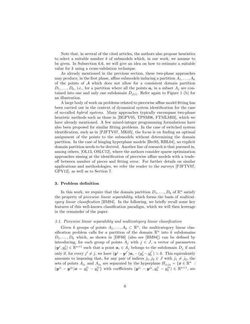
In the literature, different error functions (e.g., linear or quadratic) as wellas different types of domain partition (with linearly or nonlinearly separablesubdomains) have been considered. See Figure 1 (a) for an illustration of thecase with k = 2 and a domain partition with linearly separable subdomains.

2For greater readability, transposition symbols will be omitted throughout the paper. Ifone wanted to specify the row and column nature of the vectors that we use, ai would be acolumn vector, while wj and, in the following, yj , would be row vectors.

2

bi

aiD1D2

bi

ai

(a) (b)

Figure 1: (a) A piecewise affine model with k = 2, fitting the eight data points A = {ai}i∈Iand their observations {bi}i∈I with two submodels (in dark gray). The points (ai, bi) assignedto each submodel are indicated by � and N. The model adopts a linearly separable partitionof the domain R2 (represented in light gray). (b) An infeasible solution obtained by solving ak-hyperplane clustering problem in R3 with k = 2. Although yielding a smaller fitting errorthan that in (a), this solution induces a partition A1, A2 of A where the points ai assigned tothe first submodel (indicated by �) cannot be linearly separated from those assigned to thesecond submodel (indicated by M). In other words, the solution does not allow for a domainpartition D1, D2 of R2 with linearly separable subdomains that is consistent with the pointpartition A1, A2.

In this work, the focus is on the version of the general piecewise affine modelfitting problem with a linear error function (`1 norm) and a domain parti-tion with piecewise linearly3 separable subdomains. We refer to it as to thek-Piecewise Affine Model Fitting with Piecewise Linear Separability problem(k-PAMF-PLS). A more formal definition of the problem will be provided inSection 3.

k-PAMF-PLS shares a connection with the so-called k-Hyperplane Cluster-ing problem (k-HC), an extension of a classical clustering problem which callsfor k hyperplanes in Rn+1 which minimize the sum, over all the data points{(a1, b1), . . . , (am, bm)}, of the `2 distance from (ai, bi) to the hyperplane thepoint is assigned to. See [BM00, AC13, Con11, Con15] for some recent workon the problem and [ADC13] for the problem variant aiming at minimizing thenumber of hyperplanes needed to fit all the points within a prescribed toler-ance ε > 0.

It is nevertheless crucial to note that, differently from many of the approachesin the literature (which we briefly summarize in Section 2) and depending onthe type of the domain partition that is adopted, a piecewise affine functioncannot be determined by just solving an instance of k-HC. A naive applicationof algorithms designed for k-HC to tackle k-PAMF-PLS can indeed lead tosolutions with a large fitting error, as a consequence of the domain partitioning

3Although this kind of separation employs piecewise affine functions, it is usually referredto, in the literature, as piecewise linear. We will do so also here for uniformity with previouswork.

3

aspect being entirely neglected. As illustrated in Figure 1 (b), the two aspectsof k-PAMF-PLS, namely, submodel fitting and domain partitioning, should betaken into account at once to obtain a solution where the two are consistent.For this reason, most of the algorithms in the literature incorporate techniquesto enforce the piecewise linear separability of the domain, typically after firstsolving k-HC (or one of its variants). In this work, we propose exact methods fork-PAMF-PLS based on mixed-integer linear programming as well as heuristicalgorithms which consider both aspects of the problem simultaneously, ratherthan deferring the domain partitioning aspect to a later stage of the solutionprocess.

The paper is organized as follows. After summarizing previous and relatedworks in Section 2, we formally define the problem under consideration in Sec-tion 3. In Section 4, we provide a Mixed-Integer Linear Programming (MILP)formulation for k-PAMF-PLS. We then strengthen the formulation when usingit for solving the problem in a branch-and-cut setting by generating symmetry-breaking constraints. In Section 5, we propose a four-step heuristic to tacklelarger-size instances. Computational results are reported and discussed in Sec-tion 6. In Section 7, we consider the application of k-PAMF-PLS to problemsin the area of dynamical system identification and compare the obtained re-sults with those provided by state-of-the-art methods. Section 8 contains someconcluding remarks. Portions of this work appeared, in a preliminary stage,in [ACT11, ACT12].

2. Previous and related work

Recently, there has been a growing interest in mixed-integer programmingand discrete optimization approaches to a wide range of problems in the areasof data mining and statistics, see, e.g., [IR03, CSK06, BS07, CBR12, BM14,MT15]. As to the problem of fitting a piecewise affine model to data points,many variants have been considered in the literature. We briefly mention someof the most relevant ones in this section.

In some works, the domain is partitioned a priori, exploiting the domain-specific information about the dataset at hand. This approach has a typicallylimited applicability, as it requires knowledge of the underlying structure ofthe data, which may often not be available. For some examples, the reader isreferred to [TV12] (which admits the use of a predetermined domain partitionas a special case of a more general approach) and to the references therein.

In other works, a domain partition is easily derived when the attention isrestricted to convex or concave piecewise affine models. Indeed, if the model isconvex, each subdomain Dj is uniquely defined as Dj = {x ∈ Rn : fj(x) ≥fj′(x) ∀j′ ∈ J} (similarly, for concave models, with ≤ instead of ≥). This is,for instance, the case of [MB09] and [MRT05], where the fitting function is thepointwise maximum (or minimum) of a set of k affine functions. In the case ofhinging hyperplane models, see [Bre93] or [RBL04] and the references therein,the domain partition does not need to be explicitly derived due to the specialstructure of this type of piecewise affine models.

4

In more general versions of the problem, a partition of the domain has tobe explicitly derived together with the fitting submodels in order to obtain apiecewise affine function from Rn to R. To the best of our knowledge, mostof the available methods are two-phase in nature, in that they split the prob-lem into two subproblems that are solved sequentially: i) a clustering problemaiming at partitioning the data points and simultaneously fitting each subsetwith an affine submodel, and ii) a classification problem asking for a domainpartition consistent with the previously determined submodels and the corre-sponding point partition. Note that the clustering problem considers the datapoints {(a1, b1), . . . , (am, bm)} ⊂ Rn+1, whereas the classification problem con-siders the original points {a1, . . . ,am} ⊂ Rn but not the observations bi. Theclustering phase is typically carried out by either choosing a given number k ofhyperplanes which minimize the fitting error, or by finding a minimum numberof hyperplanes yielding a fitting error of, at most, a given ε. Although suchtwo-phase approaches turn out to perform satisfactorily in several of the controlapplications that are cited in this section, in the general case they may lead tosolutions with a large fitting error (due to deferring the domain partition to theend), as also illustrated in Section 6 with our computational experiments.

Among the two-phase methods available in the literature, we first mention[BGPV05], which includes a postprocessing phase aiming at enforcing piecewiselinear separability. In its clustering phase, as proposed in [AM02], the problemof fitting the data points in Rn+1 with a minimum number of linear submodelswithin a given error tolerance ε > 0 is formulated and solved as a Min-PFSproblem, which amounts to partitioning a given infeasible linear system intoa minimum number of feasible subsystems. Then, in the classification phase,the domain is partitioned via a Support Vector Machine (SVM). In [TPSM06]the authors solve a k-hyperplane clustering problem via the heuristic proposedin [BM00], resorting to SVM for the classification phase. A similar approachis also adopted in [BS07], where, in the first phase, a k-hyperplane clusteringproblem is solved as a mixed-integer linear program and, in the second phase,the domain partition is derived via Multicategory Linear Classification (MLC).For references to SVM and MLC, see [Vap96] and [BM94], respectively. Themethod proposed in [FTMLM03] associates, to each data point ai, a hyper-plane computed by solving a least square problem over the c closest points, andthen clusters them into k groups via a weighted version of the k-means algo-rithm4 [Mac67]. To avoid grouping together hyperplanes corresponding to faraway points and, thus, partially accounting for the domain partitioning aspect,clustering is carried out in a 2n + 1-dimensional feature space which includesthe hyperplane parameters and the centroid of the c points corresponding tothe neighbourhood. Finally, SVM is applied to derive the domain partition aposteriori.

4k-means is a well-known heuristic to partition m points {a1, . . . ,am} into k groups (clus-ters) so as to minimize the total distance between each point and the centroid (mean) of thecorresponding group.

5

Note that, in several of the cited articles, the authors also propose heuristicsto select a suitable number k of submodels which, in our work, we assume tobe given. In Subsection 6.6, we will give an idea on how to estimate a suitablevalue for k using a cross-validation technique.

As already mentioned in the previous section, these two-phase approachesmay produce, in the first phase, affine submodels inducing a partition A1, . . . , Akof the points of A which does not allow for a consistent domain partitionD1, . . . , Dk, i.e., for a partition where all the points ai in a subset Aj are con-tained into one and only one subdomain Dj(i). Refer again to Figure 1 (b) foran illustration.

A large body of work on problems related to piecewise affine model fitting hasbeen carried out in the context of dynamical system identification for the caseof so-called hybrid systems. Many approaches typically encompass two-phaseheuristic methods such as those in [BGPV05, TPSM06, FTMLM03], which wehave already mentioned. A few mixed-integer programming formulations havealso been proposed for similar fitting problems. In the case of switched systemidentification, such as in [PJFTV07, MK05], the focus is on finding an optimalassignment of the points to the submodels without determining the domainpartition. In the case of hinging hyperplane models [Bre93, RBL04], no explicitdomain partition needs to be derived. Another line of research is that pursued in,among others, [OL13, OSLC12], where the authors consider sparse optimizationapproaches aiming at the identification of piecewise affine models with a trade-off between number of pieces and fitting error. For further details on similarapplications and methodologies, we refer the reader to the surveys [PJFTV07,GPV12], as well as to Section 7.

3. Problem definition

In this work, we require that the domain partition D1, . . . , Dk of Rn satisfythe property of piecewise linear separability, which forms the basis of multicat-egory linear classification [BM94]. In the following, we briefly recall some keyfeatures of this well-known classification paradigm, which we will then leveragein the remainder of the paper.

3.1. Piecewise linear separability and multicategory linear classification

Given k groups of points A1, . . . , Ak ⊂ Rn, the multicategory linear clas-sification problem calls for a partition of the domain Rn into k subdomainsD1, . . . , Dk which, as shown in [DF66] (also see [BM94]) can be defined byintroducing, for each group of points Aj with j ∈ J , a vector of parameters

(yj , yj0) ∈ Rn+1 such that a point ai ∈ Aj belongs to the subdomain Dj if and

only if, for every j′ 6= j, we have (yj −yj′)ai− (yj0−yj

′

0 ) > 0. This equivalentlyamounts to imposing that, for any pair of indices j1, j2 ∈ J with j1 6= j2, thesets of points Aj1 and Aj2 are separated by the hyperplane Hj1j2 = {x ∈ Rn :

(yj1 − yj2)x = yj10 − yj20 } with coefficients (yj1 − yj2 , yj10 − yj20 ) ∈ Rn+1, see

6

D1 D2

D3

D4 D5

D1

D2

(a) (b)

Figure 2: (a) Piecewise linear separation of five linearly separable groups of points. (b)Classification with a minimum misclassification error of two linearly inseparable groups ofpoints (note the misclassified black point).

Figure 2 (a) for an illustration. It follows that, for any j ∈ J , the domain Dj isdefined as:

Dj ={x ∈ Rn : (yj − yj

′)x− (yj0 − yj

′

0 ) > 0 ∀j′ ∈ J \ {j′}}. (1)

If the group of points A1, . . . , Ak are not piecewise linearly separable, thereexists at least a point ai and a pair j1, j2 for which the inequality (yj1−yj2)ai−(yj10 − yj20 ) > 0 is violated for any choice of the vectors of parameters (yj , yj0)with j ∈ J . In this case, the typical approach is to look for a solution whichminimizes the sum, over all the data points, of the so-called misclassificationerror. For a point ai ∈ Aj(i), where j(i) is the index of the group the pointbelongs to, the misclassification error is defined as:

max

{0, maxj∈J\{j(i)}

{−(yj(i) − yj)ai + (y

j(i)0 − yj0)

}}, (2)

thus corresponding to the largest violation among the inequalities (yj(i)−yj)ai−(yj(i)0 − yj0) > 0. For an illustration, see Figure 2 (b).

Since the set of vectors (yj , yj0), for j ∈ J , satisfying constraint (yj(i) −yj)ai−(y

j(i)0 −yj0) > 0 is an open subset of Rn+1, it is common practice to replace

the constraint by the inhomogeneous constraint (yj(i)−yj)ai− (yj(i)0 −yj0) ≥ 1,

which induces a closed feasible set. This can be done without loss of generality if

we assume that the norm of the vectors (yj(i)yj(i)0 ) and (yj , yj0) can be arbitrarily

large, for all j ∈ J . Indeed, if (yj(i) − yj)ai − (yj(i)0 − yj0) > 0 but (yj(i) −

yj)ai− (yj(i)0 − yj0) < 1 for some ai ∈ A, then a feasible solution which satisfies

the inhomogeneous constraint can be obtained by just scaling (yj(i), yj(i)0 ) and

(yj , yj0) by a constant λ ≥ 1

(yj(i)−yj)ai−(yj(i)0 −yj0). The misclassification error for

the inhomogeneous version is thus:

max

{0, maxj∈J\{j(i)}

{1− (yj(i) − yj)ai + (y

j(i)0 − yj0)

}}. (3)

7

3.2. k-Piecewise affine model fitting problem with piecewise linear separability

We can now provide a formal definition of the k-Piecewise Affine ModelFitting with Piecewise Linear Separability problem.

k-PAMF-PLS: Given a set of m points A = {a1, . . . ,am} ⊂ Rnwith the corresponding observations {b1, . . . , bm} ⊂ R and a positiveinteger k:

i) partition A into k subsets A1, . . . , Ak which are piecewise lin-early separable via a domain partition D1, . . . , Dk of Rn in-duced, according to Equation (1), by a set of vectors (yj , yj0) ∈Rn+1, for j ∈ J ,

ii) determine, for each subdomain Dj , an affine function fj : Dj →R where fj(x) = wjx− wj0 with parameters (wj , wj0) ∈ Rn+1,

so as to minimize the linear error function

m∑i=1

∣∣∣bi − (wj(i)ai − wj(i)0

)∣∣∣,where j(i) ∈ J is the index for which ai ∈ Aj(i) ⊂ Dj(i).

It is worth emphasizing that, in this problem, both the domain partition andthe fitting hyperplanes have to be determined jointly.

4. Strengthened mixed-integer linear programming formulation

In this section, we propose an MILP formulation to solve k-PAMF-PLSto optimality via a branch-and-cut method, as implemented in state-of-the-artMILP solvers. To enhance the efficiency of the solution algorithm, we breakthe symmetries that naturally arise in the formulation by generating symmetry-breaking constraints, as we will explain in the following.

Our MILP is derived by combining an adapted hyperplane clustering for-mulation with a multicategory linear classification one. The former allows usto partition the data points into k subsets A1, . . . , Ak and to determine anaffine submodel for each of them (see, e.g., [AC13] or [MK05, PJFTV07] forclosely related formulations for the identification of switched systems). Thelatter guarantees a piecewise linearly separable domain partition D1, . . . Dk,consistent with the k subsets A1, . . . , Ak (see the previous section and [BM94]).Consistently with the definition of the problem, in the resulting formulation,the parameters of the fitting affine submodels and the piecewise linear domainpartition are determined simultaneously.

4.1. MILP formulation

For each i ∈ I and j ∈ J , we introduce a binary variable xij which takesvalue 1 if the point ai is contained in the subset Aj and 0 otherwise. Let zibe the fitting error of point ai ∈ A for each i ∈ I, (wj , wj0) ∈ Rn+1 be the

parameters of the submodel of index j ∈ J , and (yj , yj0) ∈ Rn+1, with j ∈ J , bethe parameters used to enforce piecewise linear separability. Let also M1 and

8

M2 be large enough constants (whose value is discussed below). The formulationis as follows:

min

m∑i=1

zi (4)

s.t.

k∑j=1

xij = 1 ∀i ∈ I (5)

zi ≥ bi −wjai + wj0 −M1(1− xij) ∀i ∈ I, j ∈ J (6)

zi ≥ −bi +wjai − wj0 −M1(1− xij) ∀i ∈ I, j ∈ J (7)

(yj1 − yj2)ai − (yj10 − yj2

0 ) ≥ 1−M2(1− xij1) ∀i ∈ I, j1, j2 ∈ J : j1 6= j2 (8)

xij ∈ {0, 1} ∀i ∈ I, j ∈ J (9)

zi ≥ 0 ∀i ∈ I (10)

(wj , wj0) ∈ Rn+1 ∀j ∈ J (11)

(yj , yj0) ∈ Rn+1 ∀j ∈ J. (12)

Constraints (5) guarantee that each point ai ∈ A be assigned to exactly one

submodel. Constraints (6) and (7) impose that zi = |bi −wj(i)ai +wj(i)0 |. This

is because, together, they imply that zi ≥ |bi − wjai + wj0| − M1(1 − xij).

When xij = 1, this amounts to imposing zi ≥ |bi −wjai + wj0| (which will betight in any optimal solution due to the objective function direction), whereasit becomes redundant (since zi ≥ 0) when xij = 0 and M1 is large enough. Foreach j1 ∈ J , Constraints (8) impose that all the points assigned to the subsetAj1 (for which the term −M2(1 − xij) vanishes) belong to the intersection of

all the halfspaces defined by (yj1 − yj2)ai − (yj10 − yj20 ) ≥ 1, whereas they aredeactivated when xij1 = 0 and M2 is sufficiently large. This way, we imposea zero misclassification error for each data point, thus guaranteeing piecewiselinear separability among the points assigned to the different submodels. Notethat, if Constraints (8) are dropped, we obtain a relaxation corresponding toa k-hyperplane clustering problem where the objective function is measuredaccording to (4), (6), and (7).

It is important to observe that, in principle, there exists no (large enough)finite value for the parameter M1 in Constraints (6) and (7). As an example,the fitting error between a point (a, b) = (e,−1) ∈ Rn+1, where e is the all-onevector, and the affine function f = wa− 1 is equal to ‖w‖1 (the `1 norm of w)and, thus, it is unbounded and arbitrarily large for an arbitrarily large ‖w‖1.Let j(i) ∈ J such that xij(i) = 1. The introduction of a finite M1 correspondsto letting:

zi = max

j=j(i) and xij(i)=1︷ ︸︸ ︷|bi −wj(i)ai + w

j(i)0 |,

j 6=j(i) and xij=0︷ ︸︸ ︷max

j∈J\{j(i)}{|bi −wjai + wj0| −M1}

, (13)

rather than zi = |bi − wj(i)ai + wj(i)0 |. Therefore, a finite M1 introduces a

9

penalization term into the objective function equal to:

m∑i=1

max

{0, maxj∈J\{j(i)}

{|bi −wjai + wj0| −M1} − |bi −wj(i)ai + wj(i)0 |

}. (14)

The effect is of penalizing solutions where the fitting error between any pointand any submodel is too large, regardless of the submodels to which each pointis assigned.

We face a similar issue with Constraints (8) due to the presence of the pa-rameter M2. Indeed, for any finite M2 and for xij1 = 0, each of such constraints

implies (yj1 − yj2)ai − (yj10 − yj20 ) ≥ 1 −M2. Hence, Constraints (8) impose

that the linear distance5 −(yj1 − yj2)ai + (yj10 − yj20 ) (notice that the signs areconsistent with Equation (3)) between each point ai and the hyperplane sepa-rating any pair of subdomains Dj1 , Dj2 be smaller than M2− 1 even if ai is notcontained in either of the subdomains, i.e., even if ai /∈ Aj1 and ai /∈ Aj2 .

In spite of the lack of theoretically finite values for M1 and M2, settingthem to a value a few orders of magnitude larger than the size of the boxencapsulating the data points in Rn+1 typically suffices to produce good quality(if not optimal) solutions. We will mention an occurrence where this is not thecase in Section 6.

4.2. Symmetries

Let X ∈ {0, 1}m×k be the binary matrix with entries {X}ij = xij for i ∈ Iand j ∈ J . We observe that Formulation (4)–(12) admits symmetric solutions asa consequence of the existence of a symmetry group acting on the columns of X.This is because, for any X representing a feasible solution, an equivalent solutioncan be obtained by permuting the columns of X, an operation which correspondsto permuting the labels 1, . . . , k by which the submodels and subdomains areindexed.

From a computational point of view, the solvability of our MILP formu-lation for k-PAMF-PLS is hindered by the existence of symmetries. On theone hand, this is because, when adopting methods based on branch-and-bound,symmetries typically lead to an unnecessarily large search tree where equiva-lent (symmetric) solutions are discovered again and again at different nodes.On the other hand, the presence of symmetries usually leads to weaker Lin-ear Programming (LP) relaxations, for which the barycenter of each set ofsymmetric solutions, which often yields very poor LP bounds, is always fea-sible [KP08]. This is the case of our formulation where, for a sufficiently largeM = M1 = M2 ≥ k

k−1 max{1, |b1|, |b2|, . . . , |bm|}, the LP relaxation of Formu-

lation (4)–(12) admits a solution of value 0. To see this, let xij = 1k for all

i ∈ I, j ∈ J . Constraints (5) are clearly satisfied. Let then zi = 0 for all i ∈ I,

5Given a point a and a hyperplane of equation wx − w0 = 0, the distance from a to the

closest point belonging to the hyperplane amounts to|wa−w0|‖w‖2

. Then, the linear distance

mentioned in the text corresponds to the point-to-hyperplane distance multiplied by ‖w‖2.

10

(wj , wj0) = (0, 0) and (yj , yj0) = (0, 0) for all j ∈ J . Constraints (6), (7), and (8)are then satisfied whenever we have, respectively, M1

k−1k ≥ bi, M1

k−1k ≥ −bi,

and M2k−1k ≥ 1.

A way to deal with this issue is to partition the set of feasible solutionsinto equivalence classes (or orbits) under the symmetry group, selecting a singlerepresentative per class. Different options are possible. We refer the readerto [Mar10] for an extensive survey on symmetry in mathematical programming.A possibility, originally introduced in [MDZ01, MDZ06], is of selecting as arepresentative the (unique) feasible solution of each orbit where the columnsof X are lexicographically sorted in nonincreasing order. According to [KP08],we call the convex hull of such lexicographically sorted matrices X ∈ {0, 1}m×korbitope.

4.3. Symmetry breaking constraints from the partitioning orbitope

Since, in our case, X is a partitioning matrix (a matrix X ∈ {0, 1}m×k withexactly a 1 per row), we are interested in the so-called partitioning orbitope,whose complete linear description is given in [KP08].

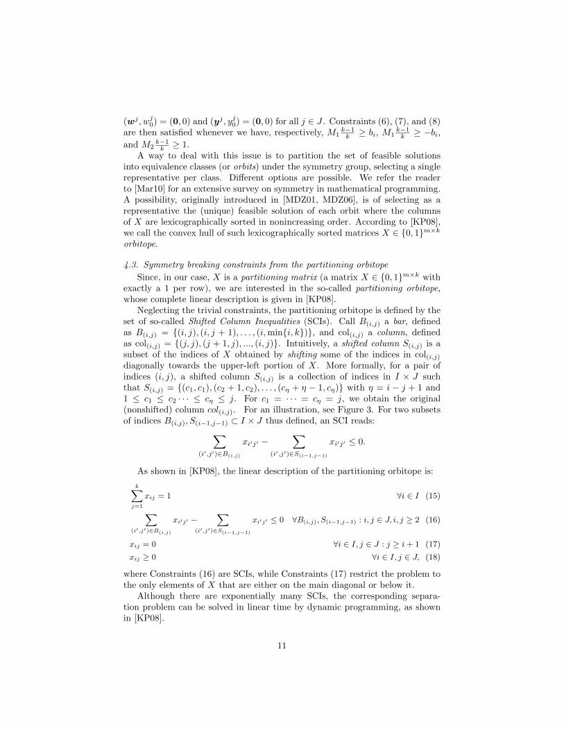
Neglecting the trivial constraints, the partitioning orbitope is defined by theset of so-called Shifted Column Inequalities (SCIs). Call B(i,j) a bar, definedas B(i,j) = {(i, j), (i, j + 1), . . . , (i,min{i, k})}, and col(i,j) a column, definedas col(i,j) = {(j, j), (j + 1, j), ..., (i, j)}. Intuitively, a shifted column S(i,j) is asubset of the indices of X obtained by shifting some of the indices in col(i,j)diagonally towards the upper-left portion of X. More formally, for a pair ofindices (i, j), a shifted column S(i,j) is a collection of indices in I × J suchthat S(i,j) = {(c1, c1), (c2 + 1, c2), . . . , (cη + η − 1, cη)} with η = i − j + 1 and1 ≤ c1 ≤ c2 · · · ≤ cη ≤ j. For c1 = · · · = cη = j, we obtain the original(nonshifted) column col(i,j). For an illustration, see Figure 3. For two subsetsof indices B(i,j), S(i−1,j−1) ⊂ I × J thus defined, an SCI reads:∑

(i′,j′)∈B(i,j)

xi′j′ −∑

(i′,j′)∈S(i−1,j−1)

xi′j′ ≤ 0.

As shown in [KP08], the linear description of the partitioning orbitope is:

k∑j=1

xij = 1 ∀i ∈ I (15)

∑(i′,j′)∈B(i,j)

xi′j′ −∑

(i′,j′)∈S(i−1,j−1)

xi′j′ ≤ 0 ∀B(i,j), S(i−1,j−1) : i, j ∈ J, i, j ≥ 2 (16)

xij = 0 ∀i ∈ I, j ∈ J : j ≥ i+ 1 (17)

xij ≥ 0 ∀i ∈ I, j ∈ J, (18)

where Constraints (16) are SCIs, while Constraints (17) restrict the problem tothe only elements of X that are either on the main diagonal or below it.

Although there are exponentially many SCIs, the corresponding separa-tion problem can be solved in linear time by dynamic programming, as shownin [KP08].

11

i

j

η

i

j

i

j

(a) (b) (c)

Figure 3: (a) The bar B(i,j) (in black and dark gray) and the column col(i−1,j−1) (in lightgray). (b) and (c) Two shifted columns (in light gray) obtained by shifting col(i−1,j−1). Notehow the shifting operation introduces empty rows.

When solving the MILP formulation (4)–(12) with a branch-and-cut algo-rithm, we generate maximally violated SCIs both at each node of the enumera-tion tree (by separating the corresponding fractional solution) and every time anew integer solution is found (thus separating the integer incumbent solution).

5. Four-step heuristic algorithm

As we will see in Section 6, the introduction of SCIs has a remarkable impacton the solution times. Nevertheless, even with them, the MILP formulation onlyallows for the solution of small to medium size instances in a reasonable amountof computing time.

To tackle instances of larger size, we propose an efficient heuristic that takesinto account, at each iteration, all the three aspects of the problem, namely,affine submodel fitting, point partition, and domain partition. At each itera-tion, the heuristic alternately and coordinately carries out a sequence of foursteps, the last two of which guarantee that the current solution always admitsa piecewise linear domain partition. Before describing the details of the foursteps, it is worth pointing out that the structure of our algorithm differs fromother heuristics (such as [BGPV05, FTMLM03]) where the domain partitioningaspect is considered directly just once, in the very last iteration. Moreover, ourmethod does not amount to just running an off-the-shelf clustering algorithm(tackling the first and second aspects of the problem) until convergence to alocal minimum, deriving a domain partition, and then feeding a refined solutionagain to the clustering method as a warm start.

We start from a feasible solution composed of a point partition A1, . . . , Ak, adomain partition D1, . . . , Dk (induced by the parameters (yj , yj0) for j ∈ J), and

a set of affine submodels of parameters (wj , wj0), for j ∈ J . At each iteration,the algorithm tries to improve the current solution by applying the followingfour steps (until convergence or until a time limit is met):

i) Submodel Fitting: Given the current point partition A1, . . . , Ak of A ={a1, . . . ,am}, determine, for each j ∈ J , an affine submodel with param-

12

eters (wj , wj0) which minimizes the linear fitting error over all the datapoints {(a1, b1), . . . , (am, bm)} ⊂ Rn+1. As we shall see, this is carried outby solving a single linear program.

ii) Point Partition: Given the current set of affine submodels fj : Dj → Rwith fj(x) = wjx − wj0 and j ∈ J , identify a set of critical data points(ai, bi) ∈ Rn+1 and (re)assign them to other submodels in an attemptto improve (decrease) the total linear fitting error over all the dataset.As described below, the identification and reassignment of such points isbased on an ad hoc criterion and on a related control parameter.

iii) Domain Partition: Given the current point partition A1, . . . , Ak of A ={a1, . . . ,am}, a multicategory linear classification problem is solved vialinear programming to either find a piecewise linearly separable domainpartition D1, . . . , Dk of Rn consistent with the current point partition or,if none exists, to construct a domain partition which minimizes the totalmisclassification error. In the latter case, i.e., when there is at least an in-dex j ∈ J for which Aj 6⊂ Dj , we say that the previously constructed pointpartition is not consistent with the resulting domain partition D1, . . . , Dk.

iv) Partition Consistency: If the current point partition and domain par-tition are inconsistent, the former is modified to make it consistent withthe latter. For every index j ∈ J and every misclassified point ai (if any)belonging to Aj (i.e., for any ai ∈ A where ai ∈ Aj and ai ∈ Dj′ , for somej, j′ ∈ J such that j 6= j′), ai is reassigned to the subset Aj′ associatedwith Dj′ .

We now describe the four steps in greater detail.In the Submodel Fitting step, we determine, for each j ∈ J , the submodel

parameters (wj , wj0) yielding the smallest fitting error by solving the followinglinear program:

min

m∑i=1

di (19)

s.t. di ≥ bi −wj(i)ai + wj(i)0 ∀i ∈ I (20)

di ≥ −bi + wj(i)ai + wj(i)0 ∀i ∈ I (21)

(wj , wj0) ∈ Rn+1 ∀j ∈ J (22)

di ≥ 0 ∀i ∈ I, (23)

where j(i) denotes the submodel to which the point ai is currently assigned.Note that this linear program, which is standard for solving regression problemsin `1-norm, decomposes into k independent linear programs, one per submodel.

Let us now consider the Point Partition step. Many clustering heuris-tics (see, e.g., [Mac67, BM00]) are based on the iterative reassignment of eachpoint ai to a subset Aj whose corresponding submodel yields the smallest fit-ting error. As shown in Figure 4 (a), and as can be confirmed computationally,

13

D1

D2

a1

ai

bi

D1

D2

a1

ai

bi

(a) (b)

Figure 4: (a) A solution corresponding to a local minimum for an algorithm where each pointis reassigned to the submodel yielding the smallest fitting error. (b) An improved solution thatcan be obtained by reassigning the point a1 in (a) which, according to our criterion, achievesthe highest ranking, to the rightmost submodel, and by updating the affine submodel fittingas well as the domain partition.

this choice is likely to lead to poor quality local minima. In our method, weadopt a criterion to help identify a set of critical points which might jeopardizethe overall quality of the current solution. The criterion is an adaptation ofthe one employed in the Distance-Based Point Reassignment heuristic (DBPR)proposed in [AC13] for the k-hyperplane clustering problem.

The idea of the criterion is to identify as critical those points which not onlygive a large contribution to the total fitting error for their current submodel, butalso have another submodel to which they can be reassigned without increasingtoo much the overall fitting error. The set of such points is determined byranking, for each subset Aj , each point ai ∈ Aj in nonincreasing order withrespect to the ratio between its fitting error w.r.t. the current submodel ofindex j(i) and the fitting error w.r.t. a candidate submodel. The latter isdefined as the submodel that best fits ai but which is also different from j(i).Formally, for each j ∈ J , the criterion ranks each point ai ∈ Aj with respect tothe quantity:

|bi −wj(i)ai + wj(i)0 |

minj∈J\{j(i)}{|bi −wjai + wj0|}. (24)

The Point Partition step relies on a control parameter α ∈ [0, 1). Givena current solution characterized by a point partition A1, . . . , Ak and the k as-sociated affine submodels, let m(j) denote, for all j ∈ J , the cardinality of Aj .At each iteration and for each submodel of index j ∈ J , dαm(j)e of the pointswith highest rank are reassigned to the corresponding candidate submodel, evenif this leads to a worse objective function value. The remaining points are sim-ply reassigned to the closest submodel (if they are not already assigned to it).Then, α is decreased exponentially, by updating it as α := 0.99ρt, for someparameter ρ ∈ (0, 1), where t is the index of the current iteration. For anillustration, see Figure 4 (b).

Since the reassignment of critical points, as identified by our criterion, in-

14

troduces a high variability in the sequence of solutions that are generated, thesearch process is stabilized by decreasing α to 0 over the iterations, thus pro-gressively shifting from introducing (for a large α) substantial changes in thecurrent solution to performing fine polishing operations (for a smaller α).

To avoid cycling effects, whenever a worse solution is found, we add thewhole set of the point-to-submodel assignments that we carried out involvingcritical points to a tabu list of short memory. We also consider an aspirationcriterion, that is, a criterion that allows to override the tabu status of a move if,by performing it, a solution with an objective function value that is better thanthat of the best solution found so far can be achieved. Since it is computationallytoo demanding to compute the exact objective function value of a solutionobtained after the reassignment of a model from a submodel to another one (asit would require to carry out the Submodel Fitting, Domain Partition, andPartition Consistency steps for each point and at each iteration), we considera partial aspiration criterion in which we override the tabu status of a point-to-submodel reassignment only if the corresponding fitting error is strictly smallerthan the value that was registered when the reassignment move was added tothe tabu list.

In the Domain Partition step, we derive a domain partition by construct-ing a piecewise linear separation of the sets A1, . . . , Ak which minimizes thetotal misclassification error. This is achieved by solving a Multicategory LinearClassification problem via the linear program proposed in [BM94]:

min

m∑i=1

ei (25)

s.t. ei ≥ −(yj(i) − yj)ai + (yj(i)0 − yjo) + 1 ∀i ∈ I, j ∈ J \ {j(i)} (26)

ei ≥ 0 ∀i ∈ I (27)

(yj , yj0) ∈ Rn+1 ∀j ∈ J, (28)

where j(i) denotes the submodel to which the point ai is currently assigned,and ei represents the misclassification error of point ai, for all i ∈ I. If thissubproblem admits an optimal solution with total misclassification error equalto 0, then the k subsets are piecewise linearly separable. Otherwise, the currentsolution contains at least a misclassified point ai ∈ Aj(i) with ai ∈ Dj forj ∈ J with j 6= j(i). Each such point is then reassigned to Aj in the Partition

Consistency step.The overall four-step algorithm, which we refer to with the shorthand 4S-

CR (4 Steps-CRiterion), starts from a point assignment obtained by randomlygenerating the coefficients of k affine submodels and assigning each point (ai, bi)to a submodel yielding the smallest fitting error (ties are broken arbitrarily).The four steps are then repeated until α = 0, while storing the best solutionfound so far. The method is then restarted until the time limit is reached.

Note that the Domain Partition step drives the search towards solutionsthat induce a suitable domain partition, thus avoiding infeasible solutions whichare good from a submodel fitting point of view but do not admit a piecewise

15

linearly separable domain partition, i.e., where Aj ⊂ Dj does not hold for allj ∈ J . Then, the Partition Consistency step makes sure that the pointpartition and domain partition are consistent at the end of each iteration.

6. Computational results

In this section, we report and discuss on a set of computational results ob-tained when solving k-PAMF-PLS either to optimality with branch-and-cut andsymmetry breaking constraints or with our four-step heuristic 4S-CR. First, weinvestigate the impact of symmetry breaking constraints when solving the prob-lem to global optimality. On a subset of instances for which the exact approach isviable, we compare the best solutions obtained with the exact algorithm (withina time limit) to those produced by our heuristic method. Then, we experimentwith 4S-CR and some variants on larger instances, and assess the impact of themain components of 4S-CR on the overall quality of the solutions it finds.

6.1. Experimental setup

Our exact formulation is solved with CPLEX 12.5, interfaced with the Con-cert library in C++. The separation algorithm for SCIs and the heuristic meth-ods are implemented in C++ and compiled with GNU-g++-4.3. SCIs are addedto the default branch-and-cut algorithm implemented in CPLEX via both a lazyconstraint callback and a user cut callback, thus separating SCIs for both in-teger and fractional solutions. This way, with lazy constraints, we guaranteethe lexicographic maximality of the columns of the partitioning matrix X forany feasible solution found by the method. With user cuts, we also allow forthe introduction of SCIs at the different nodes of the branch-and-cut tree, thustightening the LP relaxations. In 4S-CR (and its variants, as introduced inthe following), the Submodel Fitting and Domain Partition steps are carriedout by solving the corresponding LPs, namely (19)–(23) and (25)–(28), withCPLEX.

The experiments are conducted on a Dell PowerEdge Quad Core Xeon2.0 Ghz, with 16 GB of RAM. In the heuristics, we set ρ = 0.5 and adopta tabu list with a short memory of two iterations.

6.2. Test instances

We consider both a set of structured, randomly generated instances, as wellas some real-world ones taken from the UCI repository [FA13].

We classify the random instances into four groups: small (m = 20, 30, 40,50, 60, 75, 100 and n = 2, 3, 4, 5), medium (m = 500 and n = 2, 3, 4, 5), andlarge (m = 1000 and n = 2, 3, 4, 5)6. They are constructed by randomly sam-

6We do not consider instances with n = 1 since k-PAMF-PLS is pseudopolynomially solv-able in this case. Indeed, if the domain coincides with R, then the number of linear domainpartitions is, at most, O(mk). An optimal solution to k-PAMF-PLS can thus be found byconstructing all such partitions and then solving, for each of them, an affine model fittingproblem in polynomial time by linear programming.

16

pling the data points ai and the corresponding observations bi from a randomlygenerated (discontinuous) piecewise affine model with k = 5 pieces and an addi-tional Gaussian noise. First, we generate k subdomains D1, . . . , Dk by solving amulticategory linear classification problem on k randomly chosen representativepoints in Rn. Then, we randomly choose the submodel parameters (wj , wj0) forall j ∈ J and sample, uniformly at random, the m points {a1, . . . ,am} ∈ Rn.For each sampled point ai, we keep track of the subdomain Dj(i) which containsit and set bi to the value that the affine submodel of index j(i) takes in ai, i.e.,

wj(i)ai − wj(i)0 . Then, we add to bi an additive Gaussian noise with 0 meanand a variance which is chosen, for each submodel, by sampling uniformly atrandom within [ 7

10 · 31000 ,

31000 ]. For convenience, but w.l.o.g., after an instance

has been constructed, we rescale all its data points (and their observations) sothat they belong to [0, 10]n+1.

As to the real-world instances, we consider four datasets from the UCI reposi-tory: Auto MPG (auto), Breast Cancer Wisconsin Original (breast), ComputerHardware (cpu), and Housing (house). We remove data points with missingfeatures, convert each categorical attribute (if any) to a numerical value, andnormalize the data so that each point belongs to the interval [0, 10]n+1. We thenperform feature extraction via Principal Component Analysis (PCA), using theMatlab toolbox PRTools, calling the function PCAM(A,0.9), where A is the Mat-lab data structure where the data points are stored. After preprocessing, theinstances are of the following size: m = 397, n = 3 (auto), m = 698, n = 5(breast), m = 209, n = 5 (cpu), and m = 506, n = 8 (house).

All the instances are solved with different values of k, namely, k = 2, 3, 4, 5.This way, the experiments are in line with a real-world scenario where thecomplexity of the underlying model is unknown.

Throughout the section, speedup factors and average improvements will bereported as ratios of geometric means.

6.3. Exact solutions via the MILP formulations

We test our MILP formulation with and without SCIs on the small dataset,considering four figures:

• total computing time (in seconds) needed to solve the problem, includingthe generation of SCIs as symmetry breaking constraints (Time);

• total number of branch-and-bound nodes that have been generated, di-vided by 1000 (Nodes[k]);

• percent gap at the end of the computations (Gap), defined as 100 |LB−UB|10−4+|LB| ,

where LB and UB are the tightest lower and upper bounds that have beenfound; if LB = 0, a “-” is reported;

• total number of generated symmetry breaking constraints (Cuts).

The instances are solved for k = 2, 3, 4, 5, within a time limit of 3600 seconds.We run CPLEX in its deterministic mode on a single thread with default set-tings. In all the cases, we set M = M1 = M2 = 1000.

17

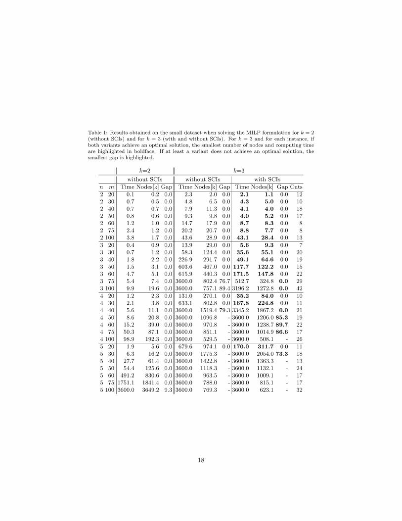
Table 1: Results obtained on the small dataset when solving the MILP formulation for k = 2(without SCIs) and for k = 3 (with and without SCIs). For k = 3 and for each instance, ifboth variants achieve an optimal solution, the smallest number of nodes and computing timeare highlighted in boldface. If at least a variant does not achieve an optimal solution, thesmallest gap is highlighted.

k=2 k=3

without SCIs without SCIs with SCIs

n m Time Nodes[k] Gap Time Nodes[k] Gap Time Nodes[k] Gap Cuts

2 20 0.1 0.2 0.0 2.3 2.0 0.0 2.1 1.1 0.0 122 30 0.7 0.5 0.0 4.8 6.5 0.0 4.3 5.0 0.0 102 40 0.7 0.7 0.0 7.9 11.3 0.0 4.1 4.0 0.0 182 50 0.8 0.6 0.0 9.3 9.8 0.0 4.0 5.2 0.0 172 60 1.2 1.0 0.0 14.7 17.9 0.0 8.7 8.3 0.0 82 75 2.4 1.2 0.0 20.2 20.7 0.0 8.8 7.7 0.0 82 100 3.8 1.7 0.0 43.6 28.9 0.0 43.1 28.4 0.0 13

3 20 0.4 0.9 0.0 13.9 29.0 0.0 5.6 9.3 0.0 73 30 0.7 1.2 0.0 58.3 124.4 0.0 35.6 55.1 0.0 203 40 1.8 2.2 0.0 226.9 291.7 0.0 49.1 64.6 0.0 193 50 1.5 3.1 0.0 603.6 467.0 0.0 117.7 122.2 0.0 153 60 4.7 5.1 0.0 615.9 440.3 0.0 171.5 147.8 0.0 223 75 5.4 7.4 0.0 3600.0 802.4 76.7 512.7 324.8 0.0 293 100 9.9 19.6 0.0 3600.0 757.1 89.4 3196.2 1272.8 0.0 42

4 20 1.2 2.3 0.0 131.0 270.1 0.0 35.2 84.0 0.0 104 30 2.1 3.8 0.0 633.1 802.8 0.0 167.8 224.8 0.0 114 40 5.6 11.1 0.0 3600.0 1519.4 79.3 3345.2 1867.2 0.0 214 50 8.6 20.8 0.0 3600.0 1096.8 - 3600.0 1206.0 85.3 194 60 15.2 39.0 0.0 3600.0 970.8 - 3600.0 1238.7 89.7 224 75 50.3 87.1 0.0 3600.0 851.1 - 3600.0 1014.9 86.6 174 100 98.9 192.3 0.0 3600.0 529.5 - 3600.0 508.1 - 26

5 20 1.9 5.6 0.0 679.6 974.1 0.0 170.0 311.7 0.0 115 30 6.3 16.2 0.0 3600.0 1775.3 - 3600.0 2054.0 73.3 185 40 27.7 61.4 0.0 3600.0 1422.8 - 3600.0 1363.3 - 135 50 54.4 125.6 0.0 3600.0 1118.3 - 3600.0 1132.1 - 245 60 491.2 830.6 0.0 3600.0 963.5 - 3600.0 1009.1 - 175 75 1751.1 1841.4 0.0 3600.0 788.0 - 3600.0 815.1 - 175 100 3600.0 3649.2 9.3 3600.0 769.3 - 3600.0 623.1 - 32

18

Table 2: Results obtained on the small dataset when solving the MILP formulation for k = 4, 5with and without SCIs. For each instance, if both variants achieve an optimal solution, thesmallest number of nodes and computing time are highlighted in boldface. If at least a variantdoes not achieve an optimal solution, the smallest gap is highlighted.

k=4

k=5

withouth

SCIs

withSCIs

withoutSCI

withSCI

nn

Tim

eNodes[k]Gap

Tim

eNodes[k]GapCuts

Tim

eNodes[k]Gap

Tim

eNodes[k]GapCuts

220

7.6

12.9

0.0

4.5

4.0

0.0

27

112.2

152.4

0.0

31.1

35.3

0.0

268

230

31.6

41.9

0.0

7.2

9.0

0.0

39

554.8

441.3

0.0

59.6

48.2

0.0

397

240

105.8

115.3

0.0

19.0

18.6

0.0

86

3600.0

1308.2

28.7

98.2

75.1

0.0

472

250

156.0

145.3

0.0

35.8

39.6

0.0

174

3600.0

1347.0

20.3

347.4

153.2

0.0

893

260

411.9

275.1

0.0

244.1

143.0

0.0

86

3600.0

865.1

90.2

1062.9

453.1

0.0

783

275

520.9

328.3

0.0

158.5

118.0

0.0

155

3600.0

577.0

97.6

2385.9

739.7

0.0

1034

2100

3600.0

673.3

15.7

367.0

169.6

0.0

233

3600.0

356.0

98.6

3600.0

319.2

98.2

1105

320

1067.9

1246.5

0.0

118.8

176.2

0.0

67

3600.0

2306.5

-2013.0

1401.2

0.0

428

330

3600.0

1590.5

-2336.6

1480.7

0.0

125

3600.0

1491.6

-3600.0

1236.9

-825

340

3600.0

1188.1

-3600.0

1344.4

34.2

91

3600.0

1077.4

-3600.0

871.3

-385

350

3600.0

896.5

-3600.0

847.6

94.4

174

3600.0

738.2

-3600.0

704.0

-496

360

3600.0

754.1

-3600.0

697.5

-120

3600.0

725.4

-3600.0

597.2

-580

375

3600.0

626.7

-3600.0

458.8

-187

3600.0

444.9

-3600.0

331.0

-843

3100

3600.0

440.5

-3600.0

370.5

-267

3600.0

324.4

-3600.0

221.4

-1691

19

The results are reported in Table 1 for k = 2, 3 and in Table 2 for k = 4, 5.In the second table, we omit the results for the instances with n = 4, 5 as, bothwith or without SCIs, no solutions with a finite gap are found within the timelimit (i.e., the lower bound LB is always 0). Note that, for k = 2, symmetry isbroken by just fixing the top left element of the matrix X to 1, i.e., by letting,w.l.o.g., x11 = 1. Hence, we do not resort to the generation of SCIs in this case.

It has recently been argued that, in a number of data mining problems, feed-ing a heuristically generated solution to the MILP solver as a warm-start mightgive a significant performance boost [BM14]. Unfortunately, when experiment-ing with this approach on k-PAMF-PLS, we only observed a negligible impact.This is arguably due to the fact that, for hard instances, most of the difficultyin proving optimality lies in improving the dual bound, and running a heuristic(to obtain a primal bound) beforehand only incurs a overhead. For this reason,we have not used this approach in our experiments.

Let us neglect the case of k = 2 and focus on the full set of 56 k-PAMF-PLSproblems that are considered for this dataset (28 instances for k = 3 and 14 fork = 4, 5). Without SCI inequalities, we achieve an optimal solution in 24 casesout of 56 (43%). The introduction of SCIs has a very positive impact. Theyallow to solve to optimality 10 more instances, for a total of 34 (60.1%). SCIsalso yield a substantial reduction in both computing time and number of nodes.When focusing on the 24 instances solved by both variants of the algorithm,the overall results show that the introduction of SCIs yields a speedup, on(geometric) average, of almost 3 times, corresponding to a reduction of 66%of the computing times. The number of nodes is reduced by the same factorof 66%. Interestingly, this improvement is obtained by adding a rather smallnumber of cuts which, in practice, prove to be highly effective. See, e.g., theinstance with m = 40, n = 3 which, when solved for k = 3 with SCIs, presentsa speedup in the computing time, when compared to the case without SCIs, of4.6 times (corresponding to a reduction of 78%) with the sole introduction of19 symmetry breaking constraints.

In our preliminary experiments, we observed the generation of a higher num-ber of cuts when employing older versions of CPLEX, such as 12.1 and 12.2whereas, with CPLEX 12.5, their number is significantly smaller. This is, mostlikely, a consequence of the introduction of more aggressive techniques for sym-metry detection and symmetry breaking in the latest versions of CPLEX. Wenevertheless remark that the improvement in computing time provided by theintroduction of SCIs appears to be comparable for all the tested versions ofCPLEX 12, regardless of the number of cuts that are generated.

Although the introduction of SCIs clearly increases the number of instanceswhich can be solved to optimality, the results in Tables 1 and 2 show thatthe exact approach via mixed-integer linear programming might require largecomputing times even for fairly small instances with n ≥ 3 and m ≥ 40 fork ≥ 4. For k = 2, all the instances are solved to optimality, with the soleexception of the instance with m = 100, n = 5 (on which we register a gap of9.3%). For k = 3, Table 1 shows that, already for n = 4 and m ≥ 50, the gapafter one hour is still larger than 80%. According to Table 2, the exact approach

20

becomes impractical for n = 3 and m ≥ 40 for k = 4, and for n = 3 and m ≥ 30for k = 5.

6.4. Comparison between the four-step heuristic 4S-CR and the MILP formu-lation

Before assessing the effectiveness of 4S-CR on larger instances, we comparethe solutions it provides with the best ones found via mixed-integer linear pro-gramming on the small dataset (within the time limit). The results are reportedin Table 3. For a fair comparison, 4S-CR is run, for the instances that are solvedto optimality by the exact method, for the same time taken by the latter. Forthe instances for which an optimal solution has not been found, 4S-CR is runup to the time limit of 3600 seconds.

When comparing the quality of the solutions found by 4S-CR with thosefound by the MILP formulation with SCIs, we register, for k = 2, very close tooptimal solutions with, on (geometric) average, a 4% larger fitting error. Thisnumber decreases to 1% for k = 3. For larger values of k, namely k = 4 andk = 5, for which the number of instances that are unsolved when adopting theMILP formulation is much larger, 4S-CR yields solutions that are much betterthan those found via mixed-integer linear programming. When neglecting theinstances with an optimal solution of value 0 (which would skew the geometricmean), the solutions provided by 4S-CR are, on geometric average, better thanthose obtained via the exact method by 14% for k = 4 and by 20% for k = 5.

For k = 2, 3, 4, 5, 4S-CR finds equivalent or better solutions that those ob-tained via mixed-integer linear programming in, respectively, 11, 15, 18, and19 cases, with strictly better solutions in, respectively, 1, 5, 16, and 15 cases.Overall, when considering the instances jointly, 4S-CR performs as good or bet-ter than mixed-integer linear programming in 63 cases out of 112 (28 instances,each solved 4 times, once per value of k), strictly improving over the latter in 37cases. This indicates that the quality of the solutions found via 4S-CR can bequite high even for small-size instances and that the difference w.r.t. the exactmethod, at least on the instances for which a comparison is viable, seems to beincreasing with the number of points m, the number of dimensions n, and thenumber of submodels k.

Note that, for the instance with m = 30, n = 3 and for both k = 2 and k = 3,the MILP formulation yields, in strictly less than the time limit, a solution whichis worse than the corresponding one found by 4S-CR. As discussed in Section 4,this is most likely due to the selection of too small values for the parametersM1 and M2. Experimentally, we observed that the issue can be avoided bychoosing M = M1 = M2 = 10000, although at the cost of a substantially largercomputing time (due to the need for a higher numerical precision to handle thelarger differences between the magnitudes of the coefficients in the formulation).

6.5. Experiments with 4S-CR and some variants

We now present and discuss the results obtained with 4S-CR and somevariants on larger instances, and assess the impact of the main features of 4S-CR (i.e., the criterion for identifying and reassigning critical points in the Point

21

Table 3: Comparison between the best results obtained for k = 2, 3, 4, 5 on the small instanceswhen solving the MILP formulation (with symmetry breaking constraints and within a timelimit of 3600 seconds) and those obtained via 4S-CR. The latter is run for as much time asthat required to solve the MILP formulation (within the time limit). For each instance, thevalue of the best solution found is highlighted in boldface.

k = 2 k = 3 k = 4 k = 5

Objective Objective Objective Objectiven m Time MILP 4S-CR Time MILP 4S-CR Time MILP 4S-CR Time MILP 4S-CR

2 20 0.1 18.3 22.4 2.1 9.6 9.6 4.5 6.1 7.1 31.1 4.5 6.12 30 0.1 30.5 30.5 4.3 19.3 19.3 7.2 10.0 10.0 59.6 7.7 8.82 40 0.5 61.3 61.3 4.1 37.8 45.4 19.0 24.7 35.5 98.2 14.8 21.22 50 0.3 56.0 56.0 4.0 39.1 40.9 35.8 26.9 29.5 347.4 22.1 22.12 60 1.2 86.6 91.7 8.7 53.1 61.8 244.1 43.2 53.1 1062.9 35.7 43.52 75 1.7 40.5 45.4 8.8 31.3 31.6 158.5 28.6 30.5 2385.9 27.3 28.42 100 1.6 114.9 114.9 43.1 62.9 62.9 367.0 48.4 48.5 3600.0 187.4 48.4

3 20 0.3 11.3 11.3 5.6 4.3 4.6 118.8 2.3 2.4 2013.0 0.4 0.93 30 0.7 14.1 13.8 35.6 9.4 9.0 2336.6 6.3 6.3 3600.0 4.5 4.73 40 2.9 29.3 32.3 49.1 19.6 21.2 3600.0 14.7 15.5 3600.0 11.7 11.73 50 2.0 48.6 55.5 117.7 26.3 26.3 3600.0 20.2 17.9 3600.0 21.2 15.13 60 4.9 40.0 40.0 171.5 22.7 25.0 3600.0 22.7 17.5 3600.0 17.3 12.93 75 5.9 72.5 82.4 512.7 43.9 47.9 3600.0 35.2 31.6 3600.0 54.0 31.53 100 10.3 86.5 88.0 3196.2 51.3 51.3 3600.0 77.2 33.6 3600.0 69.2 33.2

4 20 1.2 7.5 7.5 35.2 2.3 2.3 3600.0 0.2 0.3 2.1 0.0 0.44 30 1.2 20.0 20.3 167.8 6.8 6.8 3600.0 3.5 3.4 3600.0 1.3 1.44 40 4.1 34.4 34.4 3345.2 16.5 16.5 3600.0 11.0 10.3 3600.0 7.4 6.84 50 6.2 38.0 38.0 3600.0 20.5 20.0 3600.0 19.0 13.4 3600.0 17.7 6.34 60 12.1 40.1 41.0 3600.0 28.8 27.3 3600.0 24.8 17.9 3600.0 21.1 15.54 75 23.0 85.0 88.5 3600.0 49.4 53.9 3600.0 50.4 37.8 3600.0 46.1 32.44 100 57.0 110.3 118.0 3600.0 113.9 74.0 3600.0 139.3 49.7 3600.0 117.6 43.3

5 20 2.6 8.9 8.9 170.0 0.5 0.5 0.3 0.0 0.5 0.6 0.0 0.05 30 4.0 17.1 19.2 3600.0 6.7 6.7 3600.0 1.9 1.7 3600.0 0.3 0.65 40 12.1 37.9 41.7 3600.0 18.7 19.5 3600.0 13.3 8.9 3600.0 6.7 5.15 50 32.0 28.9 29.4 3600.0 21.7 17.9 3600.0 15.8 12.4 3600.0 9.7 8.45 60 457.1 58.4 58.6 3600.0 43.9 44.0 3600.0 37.5 31.9 3600.0 33.6 21.25 75 820.9 62.6 65.0 3600.0 26.7 29.4 3600.0 50.9 20.7 3600.0 53.0 18.45 100 3600.0 79.3 84.1 3600.0 56.0 60.8 3600.0 60.5 49.3 3600.0 61.6 42.9

22

Partition step, the Domain Partition step, and the Partition Consistency

step, applied at each iteration) on the quality of the solutions found.As already mentioned, we set ρ = 0.5 in all the experiments involving our

criterion for identifying critical points and we consider a tabu list with a memoryof two iterations. When tuning the parameters, we observed improved results onthe smaller instances when increasing ρ, as opposed to worse ones on the largerinstances. This is, most likely, a consequence of the number of iterations carriedout within the time limit, which becomes much smaller for a larger value of ρ,thus forcing the method to halt with a solution which is too close to the start-ing one. As to the tabu list, we observed that a short memory of two iterationssuffices to prevent loops. Indeed, due to the nature of the problem as well asdue to the many aspects of k-PAMF-PLS that our method considers, the valuesof the parameters of the piecewise affine submodels change often dramaticallywithin very few iterations. This way, few iterations taking place after a wors-ening move typically suffice to prevent that a point-to-submodel reassignmentcould take place twice, thus making the occurrence of loops extremely unlikely.

To assess the impact of the Point Partition step based on the criterionfor critical points (and on the corresponding control parameter), we introduce avariant of 4S-CR where, in the former step, every point (ai, bi) is (re)assignedto a submodel yielding the smallest fitting error. This is in line with the reas-signment step of many popular clustering heuristics, as reported in Sections 2and 5. We refer to this method as 4S-CL (where “CL” stands for “closest”).

To evaluate the relevance of considering, in 4S-CR, the domain partitionaspect directly at each iteration (via the Domain Partition and Partition

Consistency steps), as well as to compare 4S-CR to classical algorithms, wealso consider a standard (STD) two-phase method which, first, addresses theclustering aspect of k-PAMF-PLS and, only at the end, before halting, takes thedomain partition aspect into account, thus tackling the problem in two distinct,successive phases: a clustering phase and a classification phase. In the algo-rithm, which we consider in two versions, we iteratively alternate between theSubmodel Fitting and Point Partition steps. In the Point Partition step,we either reassign every point to the “closest” submodel (STD-CL) or to thatindicated by our criterion (STD-CR). After a local minimum has been reached,a piecewise linearly separable domain partition with minimum misclassificationerror is derived by solving only once a multicategory linear classification prob-lem via linear programming, as in Problem (25)–(28). Since STD-CL is similarto most of the standard techniques proposed in the literature, we consider itas the baseline method and compare the other methods (4S-CR, 4S-CL, andSTD-CR) to it.

For the sake of comparison, we also consider an extension of this standardmethod, STD-CL, obtained after introducing an extra third phase, based onthe refinement point-reassignment criterion proposed in [BGPV05], taking placebetween the clustering and classification phases. We refer to this algorithm asSTD-CL-B. This refinement criterion is based on the identification of so-calledundecidable points, namely, data points which lie within a maximum given errorδ ≥ 0 w.r.t., at least, two affine submodels. According to this criterion, each

23

undecidable data point ai is iteratively reassigned to the submodel to whichthe majority of the c points which are closer, in `2-norm, to ai are currentlyassigned. We remark that [BGPV05] addresses a piecewise-affine model fittingproblem where k is minimized, subject to a maximum fitting error of δ. Toadapt the criterion to k-PAMF-PLS, we set, in our experiments, δ to the averagefitting error between each data point and its current submodel. As suggestedin [BGPV05], we select c = 10 and carry out the reassignment of undecidablepoints 5 times, each time followed by a Submodel Fitting step7.

The results for the medium, large, and UCI datasets, obtained within atime limit of, respectively, 900, 1800, and 900 seconds, are reported in Table 4.The comparison shows that 4S-CR outperforms the baseline method STD-CLin almost all the cases. When considering the medium instances, 4S-CR yieldsan improvement in objective function value of, on geometric average, 8%, 21%,21%, and 24% for, respectively, k = 2, 3, 4, and 5. On the large instances, theimprovement is of 16%, 24%, 29%, and 24%. For the four UCI instances, theimprovement is of 6%, 9%, 13%, and 16%. When considering the three datasetsjointly, the improvement is of 8%, 21%, 21%, 24%. On geometric average, forall the values of k, 4S-CR improves on the fitting error of STD-CL by 20%. Ona total of 112 instances (for the different values of k) of k-PAMF-PLS, 4S-CRachieves the best solution in 103 cases (92%).

When comparing 4S-CL to STD-CL, we register, on geometric mean andfor the different values of k, an improvement of 4%, 9%, 10%, and 16% on themedium instances, of 12%, 17%, 17%, and 11% on the large ones, and of 4%,9%, 10%, and 16% on the UCI datasets. When considering all the datasets andall the values of k jointly, the improvement is of 12%. Although still substantial,this value is not as large as that for 4S-CR, thus highlighting the relevance of ourcriterion based on critical points which is adopted in the Point Partition step.At the same time, it also shows that, even without the criterion, the central ideaof 4S-CR (i.e., considering the domain partition aspect of the problem directlyat each iteration, rather than deferring it to a final phase) has a large positiveimpact on the solution quality.

Most interestingly, the results for STD-CR are quite poor. When consid-ering all the 112 instances (for the different values of k), the method yields,on geometric average, a 4% larger fitting error w.r.t. STD-CL. This is notsurprising as, by constructing a domain partition only at the very end of thealgorithm, the solutions that are obtained before its derivation typically containa large number of misclassified points, which yield a large negative contributionto the final fitting error. Indeed, when comparing the value of the solutionsthat are found before and after carrying out the domain partition phase at theend of the method, we register an increase in fitting error of up to 4 times for

7Experiments with δ equal to the average fitting error scaled by a factor of{0.1, 0.25, 0.50, 0.75, 1} revealed that the best results are obtained with a factor of 1. Wealso experimented with c = 5, 20, 50 and carrying out 1, 10, and 20 passes of the criterion. Onaverage, on average, we obtained comparable results.

24

Table 4: Results obtained with 4S-CR, when compared to STD-CL, STD-CR, 4S-CL, andSTD-CL-B on the medium, large, and UCI instances, within a time limit of, respectively, 900,1800, and 900 seconds, for k = 2, 3, 4, 5. For each instance, the value of the best solutionfound is highlighted in boldface.

k=

2k

=3

k=

4k=

5

nm

ST

D-

ST

D-

4S

-CL

4S

-CR

ST

D-

ST

D-

ST

D-

4S

-CL

4S

-CR

ST

D-

ST

D-

ST

D-

4S

-CL

4S

-CR

ST

D-

ST

D-

ST

D-

4S

-CL

4S

-CR

ST

D-

CL

CR

CL

-BC

LC

RC

L-B

CL

CR

CL

-BC

LC

RC

L-B

medium

2500

658.6

863.4

659.7

592.7

658.7

660.2

734.7

592.7

472.9

660.2

638.3

790.6

485.8

345.7

610.8

638.3

784.9

493.1

472.9

663.4

2500406.2

406.2

406.2

406.2

406.2

400.1

400.1

400.1

274.1

400.1

416.8

416.8

387.8

254.0

416.8

416.8

400.1

383.6

254.0

416.8

2500

408.5

408.5

408.4

408.4

408.5

365.6

292.7

394.3

267.4

408.6

288.7

265.4

325.6

266.7

281.0

330.5

424.4

325.6

226.3

329.1

3500

392.1

386.7

378.7

358.2

391.8

334.0

346.1

310.7

279.2

334.6

318.6

319.9

309.9

286.6

329.8

345.5

351.0

310.5

281.3

288.4

3500

518.3

484.1

472.9

448.5

506.8

500.3

371.6

300.0

262.7

501.3

496.2

511.8

288.2

257.4

494.9

491.3

533.3

292.4

256.8

408.1

3500

699.7

698.6

580.4

574.6

750.0

612.2

627.9

508.8

447.1

522.9

502.1

548.1

447.9

449.3

459.0

532.7

564.3

411.1

427.6

503.0

4500

421.1

426.6

412.2

403.7

424.6

378.0

392.0

334.1

325.3

360.3

308.4

325.2

268.8

260.2

295.8

328.1

339.1

206.2

193.0

234.0

4500

669.0

670.0

643.0

623.8

668.5

536.6

521.1

505.5

474.3

546.2

435.5

492.3

395.7

375.2

394.8

423.4

429.2

377.2

318.8

339.4

4500

642.2

625.2

587.0

569.3

641.6

553.9

516.2

528.5

513.2

597.5

550.9

580.9

474.9

493.1

539.9

566.9

566.9

479.5

472.4

534.2

5500

531.7

511.6

520.5

503.9

531.7

381.8

403.2

370.4

360.8

368.5

280.4

348.2

264.0

242.8

288.9

277.6

278.7

230.3

264.7

288.7

5500

373.9

399.0

371.4

344.9

384.4

257.3

388.7

261.0

252.3

257.3

246.1

273.9

240.7

230.5

241.8

232.0

298.9

237.7

218.8

233.8

5500

635.1

616.0

603.4

593.7

626.1

610.4

592.0

536.4

509.8

605.9

449.3

616.0

472.5

421.7

456.6

441.4

620.6

464.5

489.0

426.0

large

21000654.5

654.5

654.5

654.5

654.5

654.1

654.1

572.5

572.5

654.1

654.6

670.0

572.5

557.6

654.6

565.7

644.5

572.5

557.8

565.7

21000

1685.4

1618.5

1452.5

1241.9

1685.4

1685.4

916.0

931.0

790.5

1685.4

1715.6

1994.0

931.0

581.6

1918.1

1208.2

1903.3

931.0

647.8

1504.8

21000

1423.0

1042.1

1019.9

953.2

1423.0

1102.5

970.6

849.1

634.3

1124.7

1190.9

1405.6

809.0

501.1

1195.7

953.2

1289.1

752.0

490.1

1233.1

31000

1371.2

1127.6

1095.8

976.8

1397.5

1182.8

1053.2

743.2

729.7

1196.6

780.3

1089.1

732.0

621.9

1041.5

1003.7

1132.4

714.2

605.7

1075.6

31000

1099.5

1072.9

1023.5

935.8

1099.5

969.5

1010.8

953.6

829.5

974.8

997.3

1014.7

934.8

793.6

1022.0

957.3

1047.9

943.4

654.5

1033.6

31000

1545.1

1408.3

1107.6

1084.2

1545.1

1217.2

1171.3

853.9

805.0

1172.7

1152.5

1209.7

777.9

536.4

1145.5

919.5

1258.6

777.9

616.5

993.0

41000

520.1

516.2

519.4

503.9

520.1

520.1

547.7

481.1

422.3

520.1

520.1

557.3

438.2

455.0

537.7

503.7

514.3

483.1

443.1

536.1

41000

672.8

672.6

666.0

655.0

672.8

536.9

544.7

502.9

480.8

518.6

500.7

513.8

481.9

450.9

484.4

511.2

521.9

478.5

463.6

484.3

41000

1154.7

1076.1

951.0

924.1

1154.7

963.3

979.4

854.6

797.7

984.5

869.5

895.1

705.8

625.1

765.3

928.0

950.6

758.5

710.4

794.2

51000

1174.6

1165.9

1110.6

1092.8

1185.5

1079.3

1061.9

972.2

941.1

1073.8

910.1

883.1

861.4

846.0

868.6

915.8

1049.4

880.2

856.1

793.9

51000

985.3

936.9

878.6

859.3

994.5

760.3

912.1

704.9

685.8

785.1

671.9

689.2

641.4

614.7

654.5

671.2

717.1

656.9

646.8

631.8

51000

570.3

568.1

573.2

565.2

579.2

487.7

531.5

491.3

471.5

488.2

474.0

521.2

469.9

464.5

481.6

481.4

486.5

476.2

451.3

481.2

UCIauto

3397

23.0

23.0

22.6

22.1

23.8

21.2

23.9

21.0

20.8

21.5

21.2

23.9

19.5

19.7

21.9

21.0

23.3

18.2

19.1

21.6

breast

5698

40.0

35.7

40.0

35.7

40.0

35.7

33.6

35.7

33.6

36.1

35.7

33.6

35.7

31.5

35.7

35.7

33.6

33.6

31.5

35.7

cpu

5209

28.0

28.2

27.6

27.0

27.9

25.2

27.5

23.4

22.2

25.8

24.4

29.2

21.6

20.7

26.2

25.9

29.2

21.0

20.1

25.5

house

8506

142.6

145.9

135.5

134.9

142.1

132.8

146.6

114.6

112.4

134.1

131.1

150.1

110.0

107.0

135.5

135.4

134.5

103.8

106.7

135.4

25

both STD-CR and STD-CL. This suggests the lack of a strong correlation, inboth algorithms, between the quality of the solutions found before and afterconstructing the final domain partition. Also note that, with the adoption ofour criterion for the identification of critical points, the Point Partition stepbecomes more time consuming. Indeed, our experiments show that the averagenumber of iterations carried out in the time limit by STD-CR with respect tothose for STD-CL can be up to 40% smaller (as observed for the large instanceswith k = 5). Therefore, investing more computing time in a more refined crite-rion for the Point Partition step turns out to be not effective for a method(such as STD-CR) which only considers the domain partition aspect in a secondphase.

The comparison between 4S-CR and STD-CL-B yields results that are com-parable to those between 4S-CR and STD-CL. Indeed, when focusing on STD-CL-B, we register a slight improvement w.r.t. STD-CL only for k = 5, equalto 2% on average. For k = 3, 4, the results of STD-CL-B and STD-CL are, onaverage, identical. For k = 2, those for STD-CL-B are slightly inferior thanthose for STD-CL, with the former method providing a fitting error 1% larger.Overall, when considering the whole dataset and all the values of k, STD-CL-Bprovides an improvement over STD-CL of less that 0.5% on average.

6.6. Generalization for different values of k

While a thorough evaluation of the accuracy and generalization capabilitiesof the models obtained with k-PAMF-PLS lies outside of the scope of this work,we carry out a cross-validation to estimate the so-called generalization error,i.e., the fitting error of the models corresponding to the solutions found withour techniques on unseen data.

We compare the results obtained with k-PAMF-PLS on the UCI instancesfor increasing values of k. As baseline for the comparisons, we also report theresults obtained when fitting a single affine model (k = 1) by minimizing the`1-norm error (this linear program is solved with CPLEX). Since these k-PAMF-PLS instances are larger than those we tackled with our exact formulation (seeTables 1,2 and Subsection 6.3) and solving them with our MILP formulationwould require too much computing time, for k ≥ 2 we take the best solutionsfound via our heuristic 4S-CR in 900 seconds.

Each data set is randomly split into two parts, with 75% of the data usedfor training and the remaining 25% retained for validation. The training set isused to compute an optimal k-PAMF-PLS model for each method, whereas theremaining points in the validation set are only used a posteriori as unseen datato evaluate the generalization error.

We construct 5 training/validation splits by sampling the data points atrandom and solve k-PAMF-PLS for each split. In Table 5, we report, for boththe training set and the validation set, the `1-norm fitting error divided by thenumber of data points (the so-called mean absolute error), averaged over the 5training/validation splits. The best result obtained in the validation phase ishighlighted in boldface.

26

Table 5: Mean absolute error of k-PAMF-PLS solutions on the of UCI dataset for k =1, 2, 3, 4, 5. Five data splits are considered to generate training and validation sets containing75% and 25% of the data points. The results are reported on average for the different valuesof k, with the best error on the training set highlighted in boldface for each instance.

k 1 2 3 4 5Train Valid Train Valid Train Valid Train Valid Train Valid

auto 0.073 0.076 0.054 0.060 0.051 0.062 0.048 0.066 0.046 0.073breast 0.263 0.285 0.052 0.070 0.047 0.074 0.046 0.077 0.044 0.089cpus 0.186 0.243 0.117 0.219 0.096 0.210 0.086 0.213 0.081 0.244hous 0.345 0.378 0.257 0.324 0.219 0.292 0.208 0.360 0.205 0.434

We observe that, as expected, the fitting error over the training sets decreasesmonotonically for larger values of k. As to the generalization error, computed,by definition, on the validation set, it achieves the smallest error for low valuesof k, between 2 and 3, while, contrary to the training case, it increases for largervalues of k = 4, 5. This suggests an overfitting phenomenon where models witha small k allow for a better generalization error on the unseen data due to theirlow complexity (the so-called Occam’s razor principle). Indeed, a closer look atthe results reveals that, by employing too many affine submodels, we may obtainsolutions where some of the hyperplanes are used to fit only a small subset ofpoints with a close to zero fitting error (which is always possible if the numberof assigned points is not larger than the dimension of the feature space). Suchsolutions, as it is intuitive to see, could generalize quite badly.

7. Application to the identification of piecewise affine dynamical sys-tems

Let us consider an application of k-PAMF-PLS to the identification of hybriddynamical systems. A dynamical system is said to be hybrid if it exhibits acombination of a continuous and discrete behavior. Such models are of usein a number of practical cases to approximate the behavior of continuous, butnonlinear, systems. Adopting the standard notation, a piecewise affine systemcan be formally described by an equation of the form:

yt = g(ϕt) + et,

where yt is the output of the system at time t, ϕt is the regression vector, et iswhite noise, and g is a piecewise affine function. In piecewise affine autoregres-sive exogenous models, the vector ϕt consists of a collection of previous inputsand outputs, namely:

ϕt = [yt−1 . . . yt−nyut−1 . . . ut−nu

],

where ny and nu define the orders of the model, and ut is the input at time t.Given an input vector u and an output vector y, the problem of identifying

a piecewise affine model that best reproduces the dynamics of the underlying

27

process has been extensively studied in the system identification literature. Werefer the reader to the surveys [PJFTV07, GPV12] and the references therein,as well as to the works we cited in Section 2.

Since the identification of this type of systems can be seen as a naturaltestbed for k-PAMF-PLS, in this section we tackle this task with our exactand heuristic algorithms. In particular, we compare our exact formulation tothe MILP formulation proposed in [RBL04] for the subclass of piecewise affinemodels based on hinging hyperplanes and compare the results of our heuristic4S-CR to a state-of-the-art approach [OL13] on a real-world benchmark datasetthat has been often used in the literature.

7.1. Comparison with a MILP formulation for the identification of hinging hy-perplane models

Hinging Hyperplane (HH) models, originally introduced in [Bre93], are piece-wise affine models defined as a sum of so-called hinge functions of the formg(x) = ±max

{w+x− w+

0 ,w−x− w−0

}. The graph of a hinge function is thus

the union of two intersecting half-hyperplanes with normal vectors (w+, w+0 )

and (w−, w−0 ) which, depending on the sign, can be either convex or concave.See Figure 5 for an illustration.

g(x) = max{w+x� w+0 , w�x� w�0 }

(w+, w+0 )

(w�, w�0 )

Figure 5: A convex hinge function.

HH models provide a convenient way to represent a large subclass of piece-wise affine models, and can be effectively used in the identification of hybridsystems, as proposed in [RBL04]. After a reparameterization, an HH modelcomposed of h hinge functions can be written as:

f(x) = w0x− w00 +

h∑j=1

sj max{wjx− wj0, 0

},

where sj ∈ {−1,+1} represents the sign of the j-th hinge function. The problemof identifying an HH model (here referred to as Hinging Hyperplane Model

28

Fitting, or HHMF) can be formulated [RBL04] as the following MILP:

min

m∑i=1

zi (29)

zi ≥ bi −w0ai + w00 −

h∑j=1

sjβij ∀i ∈ I (30)

zi ≥ −bi + w0ai − w00 +

h∑j=1

sjβij ∀i ∈ I (31)

0 ≤ βij ≤M ijδij ∀i ∈ I, j ∈ J (32)

wjai − wj0 ≤ βij ∀i ∈ I, j ∈ J (33)

βij +M ij(1− δij) ≤ wjai − wj0 ∀i ∈ I, j ∈ J (34)

(w1 w10)v ≥ (w2 w2

0)v ≥ · · · ≥ (wh wh0 )v (35)

δij ∈ {0, 1} ∀i ∈ I, j ∈ J (36)

zi ≥ 0 ∀i ∈ I (37)

(wj , wj0) ∈ Rn+1 ∀j ∈ J. (38)

Consistently with the notation used throughout this paper, the data pointsare denoted by (ai, bi) ∈ Rn+1, while (wj , wj0) are the variables describing thefitting hyperplanes (in this case, hinging hyperplanes), and the nonnegativevariables zi represent the absolute error for each point i ∈ I. The auxiliary

variables βij are introduced to linearize the term max{wjx− wj0, 0

}via Con-

straints (32)–(34), whereM ij andM ij are lower and upper bounds on wjai−wj0.

We remark that, in principle, wjai − wj0 is unbounded. Since the bounds M ij

and M ij are necessary for the linearization though, they should be chosen care-fully, lest the optimality of the solution is invalidated. Constraint (35) is in-cluded to break some of the symmetries of the model, where v ∈ Rn+1 is anarbitrary vector.

Due to their structure, hinging hyperplane models are clearly a restrictionof the more general class of piecewise affine models. Quite conveniently, thesubdomains Dj are implicitly induced by the hinge functions and, therefore,they can be reconstructed analytically a posteriori, if necessary. Note also that,differently from the models found via k-PAMF-PLS, the actual number of affinesubmodels in an optimal solution of HHMF cannot be fixed a priori to an arbi-trary number, as it depends on the number of regions into which h hyperplanes

can partition the domain D. When D = R2, such number is h(h+1)2 + 1, i.e., the

maximum number of regions into which h lines divide a plane8.When comparing the formulation for HHMF to that for k-PAMF-PLS, we see

that Formulation (29)–(38) contains O(n|J |+|I||J |) variables and O(|I||J |) con-

8Usually referred to as the lazy caterer’s sequence.

29

straints, while Formulation (4)–(12) has O(n|J |+|I||J |) variables and O(|I||J |2)constraints. The HHMF formulation has a few intrinsic limitations. First of all,the sign determining the convexity or concavity of each hinging function has tobe selected in advance, and may clearly affect the quality of the model. Sec-ondly, the formulation does not allow for discontinuities in the fitted model. Toovercome these limitations, extra variables and constraints must be added, asalso mentioned in [RBL04]. Since the more general formulation thus obtained iseven more challenging to solve, we will restrict ourselves to Formulation (29)–(38), which is used in all the experiments in [RBL04].

To compare k-PAMF-PLS to HHMF, we consider the two main instancesadopted in [RBL04], neglecting the toy examples. By imposing, for both ofthem, ny = 1, nu = 1, each data point (at, bt) in the corresponding MILPformulation is defined in terms of the system inputs and outputs as:

at := [yt−1 ut−1], bt := yt.

7.1.1. Instance 1 (Example 5 in [RBL04])

Let us consider 100 data points obtained from a system whose output attime t is computed according to the bivariate HH function:

yt = −0.3 + 1.2yt−1 − ut−1 + max{1.2 + 2ut−1, 0} −max{−0.2yt−1, 0}+ et, (39)

where et is a Gaussian noise with a variance of 0.01. The data points and theoriginal HH function from which they are sampled are displayed in Figure 6.

Figure 6: The HH function in Equation (39) with 100 sampled data points.

Our MILP formulation for k-PAMF-PLS is solved in 4.6 seconds for k = 2,yielding a total absolute error of 8.67. Consider now HHMF with a single hingefunction (thus, two affine submodels). We assume that the appropriate choices1 = +1 is known, since the data comes from a mostly convex function (seeFigure 6). Formulation (29)–(38) is solved in 5.8 seconds, and the corresponding`1-norm error in the optimal solution is 8.805. It is worth noting that the k-PAMF-PLS solution achieves a better fit by allowing for a discontinuity thatcannot be reproduced with the considered HHMF formulation.

30

On this instance, HHMF is not solved to optimality for any h ≥ 2 (50.6%gap at the time limit with h = 2), suggesting that the identification of hinginghyperplane models is a difficult task even when the sign of the hinge functionsis fixed a priori. Similarly, k-PAMF-PLS becomes very challenging already fork = 3, for which CPLEX obtains a solution with 19.8% gap in 3600 seconds.

7.1.2. Instance 2 (Example 6 in [RBL04])

Let us consider an instance with 100 data points, obtained from a systemwhose output at time t is defined according to the quadratic function:

yt = −0.5y2t−1 + 0.7ut−1 + et, (40)

where et is Gaussian noise with a variance of 0.01. The data points and theoriginal quadratic function from which they are sampled are displayed in Fig-ure 7(a).

(a) (b) (c)

Figure 7: (a) The quadratic function in Equation (40) with 100 sampled data points. (b)The model estimated by solving k-PAMF-PLS for k = 2. (c) The model estimated by solvingk-PAMF-PLS for k = 3.

For k = 2, k-PAMF-PLS is solved to optimality in 5.2 seconds. With a singleconcave hinge function (we set s1 = −1 due to the nonlinear component of thefunction in Equation (40) being concave), HHMF is solved to optimality within2.4 seconds. Interestingly, the two solutions obtained with k-PAMF-PLS andHHMF have the same fitting error of 26.77, and very similar submodel equations.The solution obtained with k-PAMF-PLS is represented in Figure 7(b).

Both k-PAMF-PLS and HHMF become significantly harder when more thantwo affine submodels are considered. For k = 3, k-PAMF-PLS is solved tooptimality in 1211 seconds, yielding an error of 15.16; the optimal solution isshown in Figure 7(c). For k = 4, optimality appears out of reach within thetime limit. As far as HHMF is concerned, CPLEX does not reach optimalitywithin one hour for any value of h larger than 1 (for h = 2, we register a gap of36.4% at the time limit).

These experiments indicate that the MILP formulations for k-PAMF-PLSand HHMF are of comparable difficulty. This may be due to the fact that thebounds from the linear programming relaxations at each node of the branch-and-bound tree are, typically, rather weak.

31

7.2. System identification for a pick-and-place machine model

We now consider a real-world benchmark case study: the pick-and-place ma-chine example adopted in [BGPV05, JHFT+05, OL13]. The dataset is sampledfrom a pick-and-place machine used to place electronic components on a circuitboard. It consists of 15 seconds of input (the input voltage of the machine, u)and output (the vertical position of the mounting head, y) sampled at 4000Hz.See Figure 8 for a depiction. The physical system has two main modes: the freemode, active when the head moves freely, and the impact mode, active when thehead is in contact with the circuit board.

0

5

10

15

20

25

outp

ut

0 100 200 300 400 500 600 700

samples (time)

141210

8642

input

Figure 8: Input and output vectors u and y sampled from the pick-and-place machine.

In our experiments, we adopt the settings of [OL13] which, to the best of ourknowledge, is one of the latest references using this dataset. We will compare theresults achieved by k-PAMF-PLS to those in [OL13], obtained with a methodwhich aims at balancing the fitting error and the number of submodels via asum-of-norms regularization term. The data are downsampled to 50 Hz, so asto obtain a total of 750 samples. We consider a model of orders ny = 2, nu = 2.The data points (at, bt) are thus constructed as follows:

at := [yt−1 yt−2 ut−1 ut−2], bt := yt.

To test the effectiveness of the identification approach and assess its general-ization capabilities, we split the data set in a training and a validation set, usingthe first 8 seconds (400 points) for training and the remaining 7 seconds (350points) for validation. The validation phase is carried out by running a completesimulation of the system with the estimated model and the original input vec-tor u. Note that the task is significantly more challenging than predicting theoutput yt at time t given perfect information on the past, i.e., assuming perfectknowledge of yt−1 and yt−2. Indeed, the simulated output yt is a function (of the

32

original input and) of the simulated outputs at time t− 1 and t− 2, which werealso obtained by applying the identified piecewise affine model. Identificationerrors may clearly propagate over time.

For k = 2, our 4S-CR heuristic finds in 900 seconds a solution with a totalerror of 54.3 on the training set. When simulating the system with the inputscontained in the validation set, we obtain the output reported in Figure 9(a).Observe that this output is very similar to the solution with two affine submodelsreported in [OL13]. The fit percentage9 of our solution is 81.11%, slightly betterthan that of the solution reported in [OL13], which amounts to 78.6%.

0

5

10

15

20

25

outp

ut

0 50 100 150 200 250 300 350

time

1234

subm

odel

0

5

10

15

20

25

outp

ut

0 50 100 150 200 250 300 350

time

1234

subm

odel

(a) (b)

Figure 9: Simulation results on the pick-and-place machine example with (a) k = 2 and (b)k = 4, with real and simulated outputs reported as, respectively, a dashed and a solid line.The lower panels report the submodel that is active at each point in time.

Considering k-PAMF-PLS with k = 4 submodels, 4S-CR provides in 900seconds a solution with an objective function of 29.4 on the training set and a86.35% fit percentage in simulation, see the output in Figure 9(b). Even thougha smaller fitting error on the training set can be obtained by further increasingthe value of k, the performance in simulation (on the validation data) does notimprove for larger values of k, most likely due to overfitting. Note that thek-PAMF-PLS solution well reproduces the behavior of the system over mostof the time horizon, although the range [75, 150] appears to be particularlychallenging, as also observed in [OL13].

Overall, the experiments suggest that the techniques that we proposed tosolve k-PAMF-PLS could provide a valid alternative to state-of-the-art methodsfor piecewise affine system identification.

8. Concluding remarks

We have addressed the k-PAMF-PLS problem of fitting a piecewise affinemodel with a piecewise linearly separable domain partition to a set of data

9The fit percentage, computed as 100(

1− ‖ysim−ytrue‖‖ytrue−y‖

), is a measure of the fitting error,

where ysim is the vector of simulated outputs, ytrue is the vector of the original, sampledoutputs, and y is the mean of the original, sampled output. See [BGPV05] for more details.

33

points. We have proposed an MILP formulation to solve the problem to optimal-ity, strengthened via symmetry breaking constraints. To solve larger instances,we have developed 4S-CR, a four-step heuristic algorithm which simultaneouslydeals with the various aspects of the problem.

Computational experiments on a set of structured randomly generated andreal-world instances show that, with our MILP formulation with symmetrybreaking constraints, we can solve to optimality small-size instances. Our four-step heuristic provides close-to-optimal solutions for small-size instances, whilealso allowing us to tackle instances of much larger size. The results not onlyindicate the high quality of the solutions found by 4S-CR when compared tothose obtained with either an exact method or a standard two-phase heuristicalgorithm, but they also highlight the relevance of the different features of 4S-CR, suggesting to address them in a joint way to achieve high quality solutionsto k-PAMF-PLS. On the instances from the UCI repository, the results obtainedwith cross-validation confirm that low-complexity models (with a small valueof k) provide solutions with good generalization properties.

Finally, the performance of our k-PAMF-PLS exact and heuristic algorithmsis confirmed on problems arising in the field of dynamical system identification,for which, on benchmark instances from the literature, the quality of the solu-tions provided by our approaches well compares with state-of-the-art methods.

References

[AC13] E. Amaldi and S. Coniglio. A distance-based point-reassignmentheuristic for the k-hyperplane clustering problem. European Jour-nal of Operational Research, 227(1):22–29, 2013.

[ACT11] E. Amaldi, S. Coniglio, and L. Taccari. Formulations and heuris-tics for the k-piecewise affine model fitting problem. In Proc. of10th Cologne-Twente Workshop on Graphs and Combinatorial Op-timization (CTW), Frascati (Rome), Italy, pages 48–51, 2011.

[ACT12] E. Amaldi, S. Coniglio, and L. Taccari. k-Piecewise Affine ModelFitting: heuristics based on multiway linear classification. In Proc.of 11th Cologne-Twente Workshop on Graphs and CombinatorialOptimization (CTW), Munich, Germany, pages 16–19. Univer-sitat der Bundeswehr Munchen, 2012.

[ADC13] E. Amaldi, K. Dhyani, and A. Ceselli. Column generation for theminimum hyperplanes clustering problem. INFORMS Journal onComputing, 25(3):446–460, 2013.

[AM02] E. Amaldi and M. Mattavelli. The min pfs problem and piecewiselinear model estimation. Discrete Applied Mathematics, 118(1-2):115–143, 2002.

34

[BGPV05] A. Bemporad, A. Garulli, S. Paoletti, and A. Vicino. A bounded-error approach to piecewise affine system identification. AutomaticControl, IEEE Transactions on, 50(10):1567–1580, 2005.

[BM94] K. Bennet and O. Mangasarian. Multicategory discrimination vialinear programming. Optimization Methods and Software, 3:27–39,1994.

[BM00] P. Bradely and O. Mangasarian. k-plane clustering. Journal ofGlobal Optimization, 16:23–32, 2000.

[BM14] D. Bertsimas and R. Mazumder. Least quantile regression viamodern optimization. The Annals of Statistics, 42(6):2494–2525,2014.

[Bre93] L. Breiman. Hinging hyperplanes for regression, classification, andfunction approximation. Information Theory, IEEE Transactionson, 39(3):999–1013, 1993.

[BS07] D. Bertsimas and R. Shioda. Classification and regression viainteger optimization. Operations Research, 55:252–271, 2007.

[CBR12] A. Chang, D. Bertsimas, and C. Rudin. An integer optimizationapproach to associative classification. In F. Pereira, C. Burges,and L. Bottou, editors, Advances in Neural Information ProcessingSystems, volume 25, pages 269–277, 2012.

[Con11] S. Coniglio. The impact of the norm on the k-Hyperplane Clus-tering problem: relaxations, restrictions, approximation factors,and exact formulations. In Proc. of 10th Cologne-Twente Work-shop on Graphs and Combinatorial Optimization (CTW), Frascati(Rome), Italy, pages 118–121, 2011.

[Con15] S. Coniglio. On the optimization of vector norms and the k-hyperplane clustering problem: tightened exact and approximatedformulations within an approximation factor. Technical report,Lehrstuhl II fur Mathematik, RWTH Aachen University, 2015.

[CSK06] O. Chapelle, V. Sindhwani, and S. Keerthi. Branch and boundfor semi-supervised support vector machines. In B. Scholkopf,J. Platt, and T. Hoffman, editors, Advances in Neural InformationProcessing Systems, volume 19, pages 217–224, 2006.

[DF66] R. Duda and H. Fossum. Pattern classification by iteratively de-termined linear and piecewise linear discriminant functions. IEEETransactions on Electronic Computers, 15:220–232, 1966.

[FA13] A. Frank and A. Asuncion. UCI machine learning repository, 2013.http://archive.ics.uci.edu/ml.

35

[FTMLM03] G. Ferrari-Trecate, M. Muselli, D. Liberati, and M. Morari. A clus-tering technique for the identification of piecewise affine systems.Automatica, 39(2):205–217, 2003.

[GPV12] A. Garulli, S. Paoletti, and A. Vicino. A survey on switched andpiecewise affine system identification. In System Identification,volume 16, pages 344–355, 2012.

[IR03] F. Iannarilli and P. Rubin. Feature selection for multiclass discrim-ination via mixed-integer linear programming. IEEE Transactionson Pattern Analysis & Machine Intelligence, (6):779–783, 2003.

[JHFT+05] A. Juloski, W. Heemels, G. Ferrari-Trecate, R. Vidal, S. Paoletti,and J. Niessen. Comparison of four procedures for the identifi-cation of hybrid systems. In Hybrid systems: computation andcontrol, pages 354–369. Springer, 2005.

[KP08] V. Kaibel and M. E. Pfetsch. Packing and partitioning orbitopes.Mathematical Programming, Series A, 114:1–36, 2008.

[Mac67] J. MacQueen. Some methods for classification and analysis ofmultivariate observations. In Proc. of 5th Berkeley Symposium onMathematical Statististics and Probability, Los Angeles, Califor-nia, volume 1, pages 281–297. California University Press, 1967.

[Mar10] F. Margot. Symmetry in integer linear programming. InM. Junger, T. Liebling, D. Naddef, G. Nemhauser, W. Pulley-blank, G. Reinelt, G. Rinaldi, and L. Wolsey, editors, 50 Years ofInteger Programming 1958-2008, pages 647–686. Springer BerlinHeidelberg, 2010.

[MB09] A. Magnani and S. Boyd. Convex piecewise-linear fitting. Opti-mization and Engineering, 10:1–17, 2009.

[MDZ01] I. Mendez-Dıaz and P. Zabala. A polyhedral approach for graphcoloring. Electronic Notes in Discrete Mathematics, 7:178–181,2001.

[MDZ06] I. Mendez-Dıaz and P. Zabala. A branch-and-cut algorithm forgraph coloring. Discrete Applied Mathematics, 154(5):826–847,2006.

[MK05] E. Munz and V. Krebs. Continuous optimization approaches tothe identification of piecewise affine systems. In Proceedings of the16th IFAC World Congress, 2005.

[MRT05] O. Mangasarian, J. Rosen, and M. Thompson. Global minimiza-tion via piecewise-linear underestimation. Journal of Global Opti-mization, 32(1):1–9, 2005.

36

[MT15] R. Miyashiro and Y. Takano. Mixed integer second-order coneprogramming formulations for variable selection in linear regres-sion. European Journal of Operational Research, 247(3):721 – 731,2015.

[OL13] H. Ohlsson and L. Ljung. Identification of switched linear re-gression models using sum-of-norms regularization. Automatica,49(4):1045–1050, 2013.

[OSLC12] N. Ozay, M. Sznaier, C. Lagoa, and O. Camps. A sparsificationapproach to set membership identification of switched affine sys-tems. Automatic Control, IEEE Transactions on, 57(3):634–648,2012.

[PJFTV07] S. Paoletti, A. Juloski, G. Ferrari-Trecate, and R. Vidal. Identifi-cation of hybrid systems: a tutorial. European Journal of Control,13(2):242–260, 2007.

[RBL04] J. Roll, A. Bemporad, and L. Ljung. Identification of piecewiseaffine systems via mixed-integer programming. Automatica, 40:37–50, 2004.

[TPSM06] M. Tabatabaei-Pour, K. Salahshoor, and B. Moshiri. A modifiedk-plane clustering algorithm for identification of hybrid systems.In Proc. of 6th World Congress on Intelligent Control and Au-tomation (WCICA), volume 1, pages 1333–1337. IEEE, 2006.

[TV12] A. Toriello and J.P. Vielma. Fitting piecewise linear continuousfunctions. European Journal of Operational Research, 219(1):86–95, 2012.

[Vap96] V. Vapnik. The Nature of Statistical Learning Theory. Springer,1996.

37