download lesson plans - harvard-smithsonian center for

Activity 1 – Welcome—

Activity 1 -‐ Welcome to the Laboratory for the Study of ExoPlanets PURPOSE. Use your first session as an opportunity to:

Introduce students to the ExoLab website and the tools and activities they will be pursuing.

Engage students in a preliminary discussion of this exciting frontier of science

Elicit student knowledge and prior ideas about stars, planets, and the possibility of extraterrestrial life.

EDUCATIONAL OBJECTIVES. To introduce students to the project, it is important to give them time to consider their own personal relationship with the universe beyond Earth, and think about why it might be interesting to look for other worlds.

Core Concept Underpinning this Lesson: Our Sun is a star, and the stars are suns. Even the nearest star lies enormously far beyond our own solar system. Stars are orbited by planets, which may be very different worlds from ours.

SUGGESTIONS FOR LEADING THE LESSON. Welcome students to the community of planet hunters. They begin by registering on the website. As a teacher, you will receive a Guest Code from the Harvard-‐Smithsonian Center for Astrophysics. You’ll enter this to get to the registration page. You can register each or your students of have them do this themselves. The form asks each student to provide certain information, and allows them to create his or her own personal username and password for access to the telescopes. Once registered, students can explore the website. Through a class discussion, have them express their ideas about the search for extraterrestrial life on other worlds. Here are some suggested thought questions for students; you may have some of your own. Student Questions: Most of the other solar systems discovered so far are not like our own. For a moment, travel in your imagination to an alien world. Describe what you think life might be like on:

Activity 1 – Welcome—

a. A planet with one side that always faces its star. Students should realize that this would make one side very hot all the time, and the other side very cold. They should also realize that it would be permanent day on one side of the planet and permanent night on the other. Have them think about whether there might be any parts of this planet that might have conditions conducive to life. b. A rocky planet much bigger than Earth, where there’s more space on the surface and where gravity is stronger. Students might think about this question from a personal/human perspective, and imagine what it would be like to have more space for people to live, or for them to be heavier and for movements to be more difficult. They might also take a broader perspective and think about how life evolving on a planet with more gravity might look different from life on Earth. c. A much smaller rocky planet, where you’d have less space on the surface and weigh very little. Students’ answers will vary depending on whether they are thinking about this from a human perspective or from the broader perspective of potential impacts on the evolution of life. They might think about the ease with which they could move about, or about increased competition for space on this smaller world. d. A planet that is always cloudy, and there is never a clear day or night. Students might wonder if there would there be enough light on the surface to sup-‐ port life. From a human perspective, people on the surface would never have seen the stars. e. A planet with a very eccentric orbit, so that for part of the year it is extremely close to the sun and part of the year it is very far away. This question is a good opportunity to review students’ understanding of the cause of Earth’s seasons. Earth’s seasons are caused by the planet’s tilt (the orbit around the Sun is nearly round). In this example, the very eccentric orbit would cause extreme temperature differences from one part of the year to another.

Activity 2 – Modeling Lab — Page 1

Activity 2 – MODELING LAB PURPOSE. In this lab, students will use the interactive model to:

Visualize an alien solar system.

Plan their investigation.

Predict how a graph of the star's brightness versus time can be used to determine

whether a planet is present how large the planet is how fast it is moving whether the plane of its orbit is tilted as seen from Earth

EDUCATIONAL OBJECTIVES. This lab gives students experience with:

Reasoning from a model.

Translating from one representation of a system (the visual model) to another representation (a graph of brightness vs time).

Students will use their predictions later on to help them interpret their findings with the telescopes.

Core Concept Underpinning this Lesson: Models are important tools used by scientists working at the frontiers of science. A model – physical, visual, or theoretical – captures important features of the world, and helps us analyze and predict its behavior.

SUGGESTIONS FOR LEADING THE LESSON. In this activity, student will use a computer-‐based model of a solar system to predict how the brightness of their star varies as a planet transits across (eclipses) the star. Later, after they have made their actual observations, they can use the same model to begin to visualize what their alien solar system might look like. Remind students that we can't see an alien world directly, but we can see its effect on light from the star that it orbits. As students interact with the Modeling Lab, they can use the 4 numbered buttons to preview the 4 Challenge Levels before entering data in the text boxes that will go into their online journal.


The Sidebar Text at the right provides instructions and tips for thinking about how the Modeling Lab can help students interpret the results of their investigation. Make sure students see this and click on each purple header! Challenge Level 1. Have students observe the model and the sample graph. In the box provided, have them explain in their own words what the graph is showing. Note: Once they hit the Save button, they can't go back. (They can refresh the page and start over, but don't encourage this.)

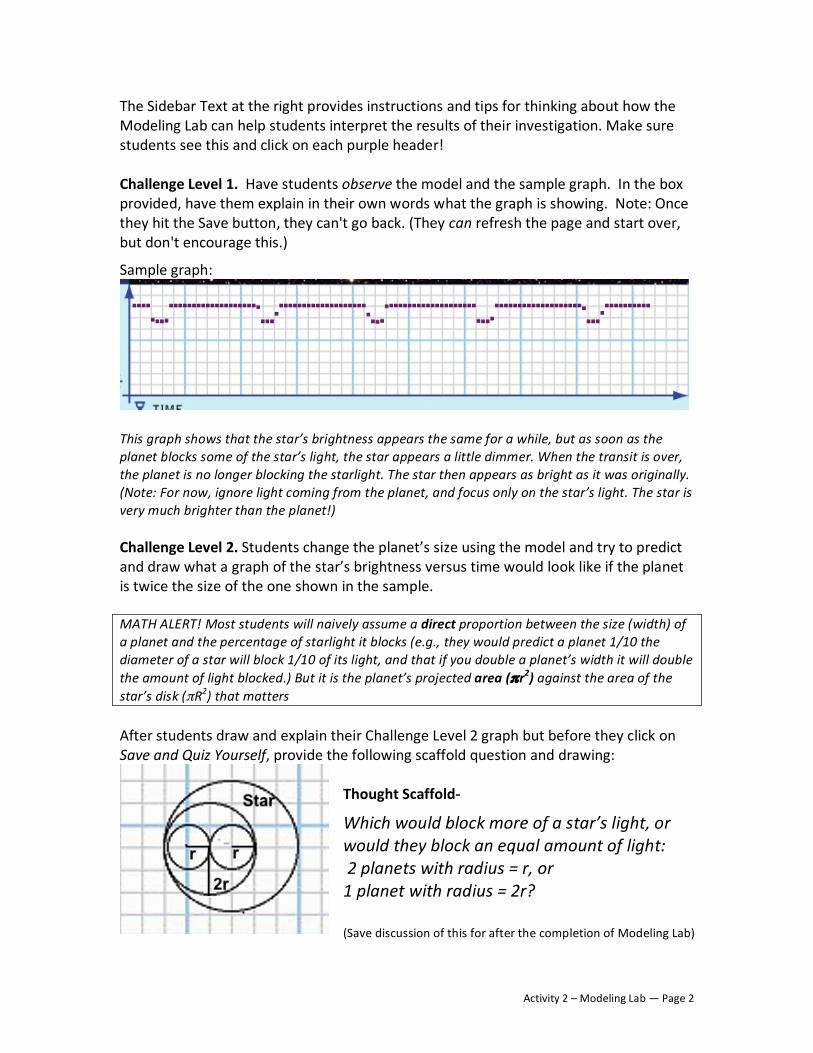
Sample graph:

This graph shows that the star’s brightness appears the same for a while, but as soon as the planet blocks some of the star’s light, the star appears a little dimmer. When the transit is over, the planet is no longer blocking the starlight. The star then appears as bright as it was originally. (Note: For now, ignore light coming from the planet, and focus only on the star’s light. The star is very much brighter than the planet!) Challenge Level 2. Students change the planet’s size using the model and try to predict and draw what a graph of the star’s brightness versus time would look like if the planet is twice the size of the one shown in the sample. MATH ALERT! Most students will naively assume a direct proportion between the size (width) of a planet and the percentage of starlight it blocks (e.g., they would predict a planet 1/10 the diameter of a star will block 1/10 of its light, and that if you double a planet’s width it will double the amount of light blocked.) But it is the planet’s projected area (πr2) against the area of the star’s disk (πR2) that matters After students draw and explain their Challenge Level 2 graph but before they click on Save and Quiz Yourself, provide the following scaffold question and drawing:

Thought Scaffold-‐

Which would block more of a star’s light, or would they block an equal amount of light: 2 planets with radius = r, or 1 planet with radius = 2r? (Save discussion of this for after the completion of Modeling Lab)


Choice B is the correct answer because a planet with twice the diameter (and radius) will block 4 times more light (r2) Challenge Level 3. Students change the speed of the orbit using the model and try to predict and draw what a graph of the star’s brightness versus time would look like if the planet’s orbit is faster than the one in the sample. If a planet has a shorter orbital period, less time will elapse between successive dips in the brightness curve. Students might also know that a planet with a longer orbital period is further away from its star, and will travel more slowly, so will block the light for longer time. Students will be presented with a series of graphs to analyze in the form of a multiple choice question. Graph C is the correct choice since the transits occur twice as frequently and the duration of each transit is shorter. Challenge Level 4. Finally, students can tilt the plane of the orbit and try to predict and draw what a graph of the star’s brightness versus time would look like if the planet’s orbit was tilted such that the planet passes across only the top portion of the star’s disk. The shape of a light curve for a planet with a tilted orbit will have slanted sides and less of a flat bottom because the planet is not fully covering the star’s disk for long. Choice B is the correct answer for the Challenge 4 quiz question. After students have answered each of the challenges, they can return to the model and change attributes to match each question. As a class, compare predictions with the graphs the Modeling Lab displays when you change the size, speed, tilt, etc. BACKGROUND INFO. Other background information you may wish to discuss: Transit of Venus What this model gets right and wrong Star is much brighter than planet Star's brightness might vary naturally with time (sunspots, flares, etc.) Planet's speed depends on distance. After the Modeling Lab, you may also want to discuss how this model might inform the overall strategy for collecting telescope data for the investigation. How long is a transit? How many images will be needed? How closely spaced? Do you need to have images that are before or after the predicted transit as well as those that might be during the transit?

Activity 3 – Telescope Lab — Page 1

TELESCOPE LAB In this brief lab, students will use the MicroObservatory telescope to take a series of images of their "target" star. These images will form the basis of students' subsequent investigation. SUGGESTIONS FOR LEADING THE LESSON. Taking an image. Explain to students that they will control the robotic telescope remotely. They will select the target star and several observing times. At night, the telescope will automatically point to the star at the requested times and will take an image. The following morning, their images will be waiting for them in the Image Lab. The image will appear as pending until the telescope actually takes the photo during the night. NOTE: All times are Arizona time, where the telescopes are located. Managing student image requests. While students can take as many or as few of the available images of the target star as they wish, you may wish to assign them to particular time slots, e.g. Students 1-‐5 request the first half hour of slots; Students 6-‐10 request the next half hour of slots, etc. That way, during the Image Lab you can more easily and efficiently have different groups of students take responsibility for measuring subsets of the data. Exposure time. Explain that each exposure time is automatically set to 60 seconds. This uniformity allows all students, in all schools, to share and compare data. (If the exposure times were allowed to differ, this would affect the measured brightness of the target star.) Opaque filter. Explain that the telescope will automatically take a so-‐called "dark image" — i.e., an image using an opaque filter that lets no light through. This image will be used to help calibrate students' measurements. As we'll see, these images will not be completely black, because the telescope itself produces some electronic noise. (In a dark room, you can see flashes and floaters produced not by any light but by the "noise" in your eyes, retinas and brain.) This dark image will be waiting for each student with their other images. Optional: Galaxy images. Students may find images of stars to be visually boring (it's just a field a white dots). To enliven the class, and to give a feeling for the immensity of the universe, have students take a few images of galaxies. Explain that the galaxies are huge collections of stars far beyond our own Milky Way galaxy. (We can't make out

Activity 3 – Telescope Lab — Page 2

individual stars in these distant galaxies. All the stars we see with the telescope are within our own Milky Way galaxy.) ABOUT THE PLANETARIUM. The interactive planetarium shows a map of the sky as it looks right now at the Arizona telescope site. You can change the time to see how the sky would look at any other time. And you can scan the sky in any direction. (Use the arrow keys or click on the map and use the mouse.) When you select a target star, the planetarium moves to the predicted location of the star for the beginning of the night’s observing run. The planetarium is also useful for seeing whether the Moon might interfere with your measurements. BACKGROUND INFO. The MicroObservatory telescope is tiny compared to the world's largest telescopes, but it can see a billion light-‐years into space. This telescopes magnifies only about 30 times, but it gathers about 500,000 times more light than your own eye can. Students’ images have captured light from a vast expanse of the cosmos, even though the telescope’s field of view is only one twenty-‐thousandth of the night sky. A galaxy in a MicroObservatory telescope image is likely to span a distance of 100,000 light years, and each star in the galaxy is an average of 5 light years (30 trillion miles) apart. The stars within the galaxy glow so brightly that we can see the galaxy’s graceful form from Earth. Yet, at the scale of students’ images, each star is smaller than an atom!

Activity 4 – Image Lab — Page 1

IMAGE LAB PURPOSE. In this lab, students will attempt to detect an alien world, by looking for a dimming of the star’s light as the planet passes in front. Students will:

Inspect the images that they took with the telescope, working only with images unmarred by clouds. Identify their target star and two comparison stars, using a star chart provided. Measure the brightness of their star in each image, along with the brightness of two comparison stars. Plot the (relative) brightness of their star, compared to the comparison stars, for each image. Inspect the resulting graph (“light-‐curve”), to see if they detect a dip in the star’s brightness that might indicate a transiting planet.

In part two of this lab, students will become “data detectives,” to see if they can use the tools provided to:

Identify areas of concern in their data—that is, “messy” parts of their graph that might call for explanation. Identify the factors that might account for the messiness in their graph (such as clouds, altitude above the horizon, moonlight, etc.)

EDUCATIONAL OBJECTIVES. This lab provides superb opportunities to highlight specific science practices that are important throughout the sciences. As a result of this lab, students should be able to:

Explain the importance of calibrating (“zeroing”) their instrument. Explain the use of a control group or internal control. Identify significant features (i.e. the transit) in their authentic data.


Identify unexpected or discordant features in their data, and explain the environmental factors and sources of error that might account for these features.

SUGGESTIONS FOR LEADING THE LESSON. Introduce the Lab. Have students look at one of their images. (On the ANALYZE IMAGES menu, press Show List, then select an image.) Expand their imaginations: These dots are stars, many of them orbited by planets — alien worlds that may or may not have life on them. Explain what is amazing about this Lab: You will be able to detect a planet and tell something about it, just from measuring the starlight. Remind students that a planet is much smaller than its star, so they are looking for a tiny dip in the star’s light — a few percent at most. Detecting the planet requires precision measurements, so students should work carefully. Explain how brightness is measured. Have students move the mouse cursor over their image. The readout at the bottom of the image shows the brightness of each pixel. The brightness comes in 4096 grey levels, ranging from 0 (black pixel) to 4095 (white pixel). The brightness number is directly proportional to the amount of light that fell on the telescope’s light-‐sensing chip. (E.g. a pixel with brightness 1500 received three times as much light as a pixel with brightness of 500.) The brightness numbers have no units: That’s fine, because we are only interested in comparing brightnesses among objects and over time—not in determining the absolute amount of light the telescope received. Examine the brightness number below the magnifying window. It measures the total brightness of all the pixels inside the yellow circle. By positioning a star within the circle, we can get a standard measurement—the brightness within a circle whose size is the same for all students and all classrooms. This lets us combine our data across observers. Explain to students how they will correct for certain errors. Explain that the target star is not the only thing that will contribute to our light measurement. Like every measuring instrument, the telescope's light-‐sensing chip itself adds "noise" to the measurement. We'll have to subtract this noise from our measurement. How do we know how much the telescope itself contributes? Simple: We take an image with an opaque filter that lets no light through ("Dark Image"). The resulting image represents the contribution from the telescope's light sensor. To see this, have students open the Dark Image (which may be at the bottom of the list target images) and run their cursor over it. Note that the brightness of every pixel is not zero. Evidently, the light-‐sensor adds its own contribution to our measurement of


brightness. In a moment, we'll see how to subtract this image from our star images, simply by pressing Subtract Dark. First, have everyone open the first class image of your star. Have students notice the typical level of brightness of the pixels. Now click the Subtract Dark button and notice what happens:

The brightness levels drop: The dark image has been subtracted, pixel by pixel, from our star image. Now the brightness display shows the brightness coming to us from the sky—not from the telescope noise. The image looks "cleaner" as well, since we have subtracted contributions from the chip's imperfections.

The dark image will automatically be subtracted from every image during your session. You do not have to worry about it again—unless you refresh the page or go to another page. (An alert will warn you if you try to Calculate and Record a measurement without having loaded a Dark Image and pressed Subtract Dark at the start of your session.) Explain to students that the Dark Subtract is a way of "zeroing" or calibrating their instrument—something done with all scientific instruments, such as pH meters, electronic scales and balances, spectrometers, etc. Background and Tips for Supporting Student Understanding:

Of the billions of stars in our Milky Way galaxy that are expected to have planets orbiting them, only a few dozen of the closest stars have actually been observed to have planets transiting across them. You are going to explore one of them. You might think this would be easy: The star is bright for a while, and then dimmer when the planet blocks some of its light. What could be easier to detect? One problem is that planets are much smaller than stars, so they block out only a few percent — at most — of the star’s light. The giant planets you’ll detect block out about 2% of their star’s light. (The Earth would block out a mere 0.01% of the Sun’s light during a transit!) Another challenge is that there are many competing factors and sources of error that students explore in this Lab.

Teaching Tips:

Before students start taking measurements, have them check to make sure they are using images of good quality. Smeared or unclear images can give bad measurements and make it hard to see a dip in the transit graph. If there are doubts about an image, have students watch the “What’s Wrong With My Image?” tutorial (available on the Wiggio ExoLab group website for teachers).


Students should follow the directions on the Image Lab to analyze the images they have taken. The measurement tutorial is a good place to start. Students will first need to subtract a dark image and then for each image will need to measure their target star, two comparison stars and two dark patches of the night sky. The computer will calculate the relative brightness of the target star. So they fully understand this process, students should do the calculations by hand for one image. After they have measured each of the components (target star, comparison stars and background) they should follow these steps to calculate a corrected brightness ratio.

1. What is the average brightness of a background sky patch? (Take the average of your two measurements.)

2. Subtract this background brightness from each of the three star brightness measurements (target star, two comparison stars).

3. Calculate the average corrected brightness of the two comparison stars. (Take the average of your two comparison star brightnesses above)

4. Compare your target star with the average of the comparison stars. What is the ratio of their brightnesses? (Divide your corrected target star brightness by your corrected average comparison star brightness)

Now ask students to click on the Calculate and Record button of the Image Lab to compare their results with the computer.

On the Graph Brightness tab students will be asked to examine their graph to assess the quality of their data. They will be asked to identify the "messy" features in their graph and then to draw on the evidence at hand to identify factors that might be responsible. Students will also look at a second set of data and asked to hypothesize why this data might look different from theirs, given that it is the same star and planet they are investigating.

Students will then follow the directions on the Graph Brightness tab to use tools (Components and Altitude) to analyze the two graphs. They will examine factors that commonly interfere with their brightness measurements:

•Time of night. (As dawn approaches, the background sky brightens.)

• Altitude of the star. (Near the horizon, stars appear dimmer and the background sky brighter.)

• Clouds and haze. (Thin clouds and haze, even when not easily seen in the telescope image, brighten the night sky and increase scatter.)

• Moon. (When the moon rises, the night sky becomes brighter.)

• Intrinsic star brightness. (The dimmer the star, the lower the signal / noise ration, and the higher the scatter.)

Activity 5 – Data Lab — Page 1

DATA LAB PURPOSE. In this lab, students analyze and interpret quantitative features of their light curve to determine the size of the planet and the nature of its orbit. In doing so, students apply statistical & mathematical skills as well as their understanding of light, gravity, and the model from the Modeling Lab. Students will:

Inspect the graph (light curve) that they generated in the Image Lab, and consider how confidently they can conclude that they’ve detected a transiting planet, given noisy data.

Compare and contrast their data with additional data for the same star and consider whether this data makes them more or less confident.

Estimate the average brightness of their target star at 2 different times – 1) when the predicted exoplanet is likely NOT in front of the star (baseline), and 2) when the planet is transiting, causing the maximum dip in the star’s brightness.

Use a graphical averaging tool to get a more quantitative estimate for the baseline and transit dip brightness values and a feel for their uncertainty.

For the culmination of this Lab students will:

Interpret the light curve and its quantitative parameters to determine important features of the planet: its size, orbital tilt, and distance from its star.

• They’ll derive the planet’s size relative to its star from the fractional dip in the star’s brightness.

• They’ll use the shape of their light curve data to draw conclusions about the orientation of the planet’s orbit with respect to Earth’s viewpoint (edge-‐on or tilted).

• They’ll estimate the relative distance of the planet from its star based on the duration of their measured transit.

EDUCATIONAL OBJECTIVES. Like the Image Lab, this Data Lab also highlights specific science practices that are important throughout the sciences. In particular, this Lab gives students practice in dealing with uncertainty as they interpret and draw conclusions from their data. As a result of this lab, students should be able to:

Explain how all measurements have inherent uncertainty, and that every measuring instrument contributes noise (so there will always be scatter in the data when you look closely enough).


Describe how obtaining more data helps to distinguish a signal from the noise.

Identify statistical measures that can help us draw conclusions when there is scatter in the data. (We can take an average of the data, and we can assess the amount of scatter in the data, e.g. standard deviation or standard error)

SUGGESTIONS FOR LEADING THE LESSON. Introduce the Lab. As students open the Data Lab, the graph will display the communal class light curve of the star they measured in the Image Lab. (If the class investigated more than one star, you can use the “Other Stars” link to choose from a list of stars for which you have light curves.) Depending upon some of the factors you discussed in the Image Lab, your class may have a very messy light curve with a lot of scatter, or a curve with a more definitive dip amidst the scatter. Explain that finding a signal in the noise of random variation is fundamental to scientific investigations: (“Is the Earth getting warmer? Does aspirin help prevent heart attacks? Is Serena Williams’ tennis game at its peak?”). Detecting exoplanets is very challenging, with many sources of noise and random scatter – the telescope instrument contributes noise; the Earth’s atmosphere (even on the clearest of nights) distorts the light from the stars. (We can see this with our naked eye as twinkling!) Question 1: Do you have evidence for a planet? Following the directions on the Data Lab sidebar, students will begin by examining their graph, deciding if they have evidence for a transit, and rating their confidence level in their conclusion. You may want to highlight this key instruction from the sidebar: Don’t look for answers. Look for results that you can justify with the evidence you have gathered. (In real science investigations like this one, Nature doesn’t come with an answer key!) Encourage students to describe the aspects of their data that give them confidence (or not) in their results. Question 2: Would more data help? Students are then able to “Show Other’s data” to see if the addition of data points leads them to believe that they may have detected a planet orbiting its star. They can also “Show astronomers’ predicted transit” to see if their results are consistent with this prediction.* Have them re-‐rate their confidence in having detected a transit and justify their ideas in the text box. [NOTE: Pilot Teachers – the Show Others’ data button may not yet work for all planets – we’re waiting for more detections, so YOUR class data may become another classes’ comparison data]

* While the “Astronomers’ predicted transit” window should be accurate for most ExoLab planets, there are conditions under which your actual observations may reveal a slight shift – a bonus discovery for your class!


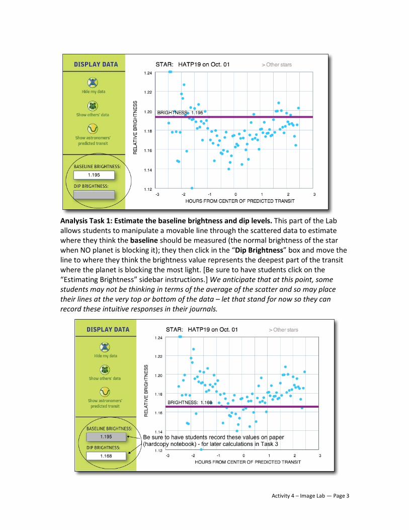
Analysis Task 1: Estimate the baseline brightness and dip levels. This part of the Lab allows students to manipulate a movable line through the scattered data to estimate where they think the baseline should be measured (the normal brightness of the star when NO planet is blocking it); they then click in the “Dip Brightness” box and move the line to where they think the brightness value represents the deepest part of the transit where the planet is blocking the most light. [Be sure to have students click on the “Estimating Brightness” sidebar instructions.] We anticipate that at this point, some students may not be thinking in terms of the average of the scatter and so may place their lines at the very top or bottom of the data – let that stand for now so they can record these intuitive responses in their journals.


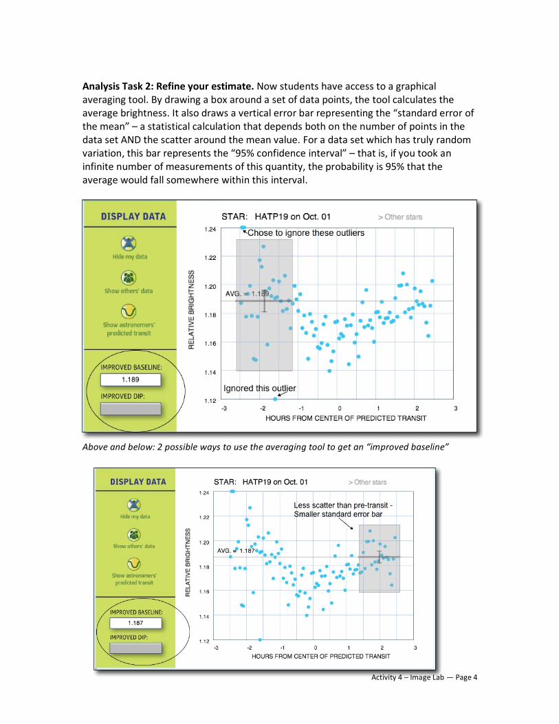
Analysis Task 2: Refine your estimate. Now students have access to a graphical averaging tool. By drawing a box around a set of data points, the tool calculates the average brightness. It also draws a vertical error bar representing the “standard error of the mean” – a statistical calculation that depends both on the number of points in the data set AND the scatter around the mean value. For a data set which has truly random variation, this bar represents the “95% confidence interval” – that is, if you took an infinite number of measurements of this quantity, the probability is 95% that the average would fall somewhere within this interval.

Above and below: 2 possible ways to use the averaging tool to get an “improved baseline”


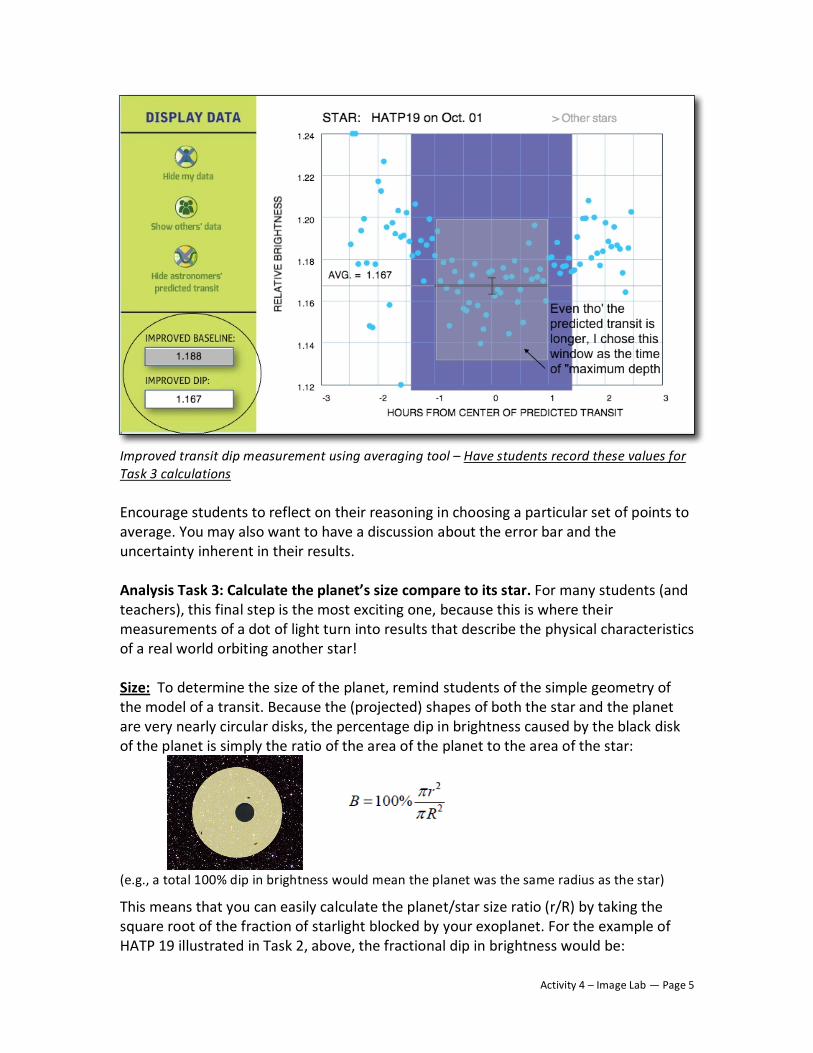
Improved transit dip measurement using averaging tool – Have students record these values for Task 3 calculations Encourage students to reflect on their reasoning in choosing a particular set of points to average. You may also want to have a discussion about the error bar and the uncertainty inherent in their results. Analysis Task 3: Calculate the planet’s size compare to its star. For many students (and teachers), this final step is the most exciting one, because this is where their measurements of a dot of light turn into results that describe the physical characteristics of a real world orbiting another star! Size: To determine the size of the planet, remind students of the simple geometry of the model of a transit. Because the (projected) shapes of both the star and the planet are very nearly circular disks, the percentage dip in brightness caused by the black disk of the planet is simply the ratio of the area of the planet to the area of the star:

(e.g., a total 100% dip in brightness would mean the planet was the same radius as the star) This means that you can easily calculate the planet/star size ratio (r/R) by taking the square root of the fraction of starlight blocked by your exoplanet. For the example of HATP 19 illustrated in Task 2, above, the fractional dip in brightness would be:


1.188 – 1.167 = 0.021 = 0.018 1.188 1.188

The square root of 0.018 = 0.13, meaning that HATP 19, according to this dataset, is 0.13 times the diameter of its star. That’s a bit larger than the size of the giant planet Jupiter, compared to the Sun. By contrast, the Earth is only 0.01 times the diameter of the Sun, so it would block out only 0.0001 of the Sun’s light (i.e. 0.01%) during a transit. To detect an Earth-‐ sized planet would require 100 times more precision than the MicroObservatory telescope.

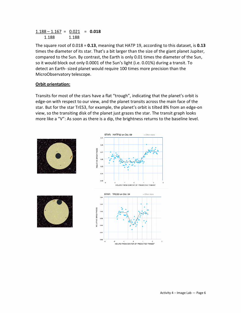
Orbit orientation: Transits for most of the stars have a flat “trough”, indicating that the planet’s orbit is edge-‐on with respect to our view, and the planet transits across the main face of the star. But for the star TrES3, for example, the planet’s orbit is tilted 8% from an edge-‐on view, so the transiting disk of the planet just grazes the star. The transit graph looks more like a “V”: As soon as there is a dip, the brightness returns to the baseline level.


Planet’s Distance from it’s Star: For this final important planetary characteristic, you’ll use Kepler’s 3rd Law, the mathematical relationship that describes how the closer a planet is to its star, the faster it moves—and so the shorter its transit time. Typically, Kepler’s law is expressed as a relationship between the period (T) of the planet (it’s year, or Time for one orbit), and the “semi-‐major axis” of its elliptical orbit, which for a circular orbit, is simply R, the distance between the star and planet. Kepler discovered that R3 = T2, where R is expressed in Astronomical Units (AU, the average Earth-‐Sun distance), and T in units of “Earth” years. In this calculation, you and your students will assume a circular orbit, and also assume that the target star is Sun-‐like (the same mass and diameter), so that you can directly compare the orbital speed and distance of your exoplanet with that of the Earth. (Of course your result will then only be approximate if the target star is not like the Sun.) Using Transit Duration and Orbital Speed to Determine Planetary Distance R While your class typically will not know the period of their planet (they would have to observe at least 2 transits in a row to determine this), they DO have the transit duration, from which they can calculate their planet’s orbital speed. If the exoplanet transits the star in, say, 3 hours, then its approximate speed (v) is simply the diameter of a Sun-‐like star (1.4 million km) divided by the transit duration (3 hrs) = 467,000 km/hr. By comparing this orbital speed with the Earth’s orbital speed (about 100,000 km/hr) Here’s how to use orbital speed, v, in Kepler’s equation rather than the period, T: It should be straightforward to see that the period (T) times the orbital speed (v) equals the orbital circumference 2πR, so that T = 2πR/v. Substituting this in to Kepler’s equation R3 = T2, we have: R3 = 4π2R2 v2 Now, you can see that the distance R is proportional to 1/v2 So…. if your exoplanet’s orbital speed is 4.7 times that of the Earth (as above), then its distance from its star is 1/(4.7)2 or 0.045 AU! The importance of this distance is that it bears on whether the planet might be habitable. The planets detected in this project are all very close to their stars. Liquid water would not exist on these planets, and neither would life.

Don’t forget to reflect on what is amazing about this Lab: You were able to detect a planet and tell something about it, just from measuring the starlight!

download lesson plans - harvard-smithsonian center for

Documents