Z. Feng MTU EE5780 Advanced VLSI CAD8.1
EE5780 Advanced VLSI CAD
Lecture 8 Interconnect Modeling and AnalysisZhuo Feng
Z. Feng MTU EE5780 Advanced VLSI CAD8.2
Introduction■ Chips are mostly made of wires called interconnect
► In stick diagram, wires set size► Transistors are little things under the wires► Many layers of wires
■ Wires are as important as transistors► Speed► Power► Noise
■ Alternating layers run orthogonally
Z. Feng MTU EE5780 Advanced VLSI CAD8.3
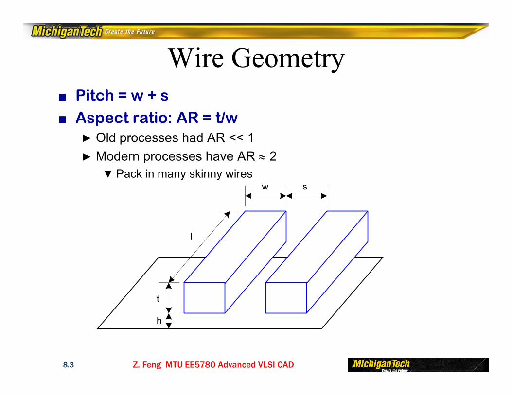
Wire Geometry■ Pitch = w + s■ Aspect ratio: AR = t/w
► Old processes had AR << 1► Modern processes have AR 2
▼Pack in many skinny wires
l
w s
t
h
Z. Feng MTU EE5780 Advanced VLSI CAD8.4
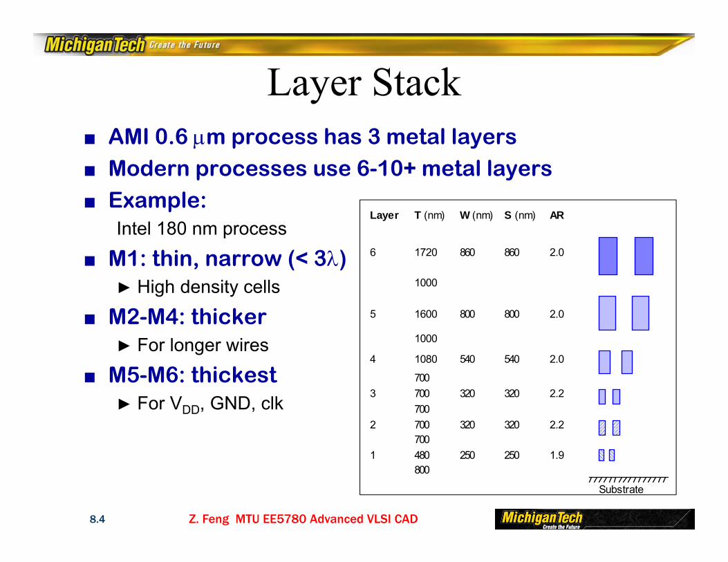
Layer Stack■ AMI 0.6 m process has 3 metal layers■ Modern processes use 6-10+ metal layers■ Example:
Intel 180 nm process
■ M1: thin, narrow (< 3)► High density cells
■ M2-M4: thicker► For longer wires
■ M5-M6: thickest► For VDD, GND, clk
Layer T (nm) W (nm) S (nm) AR
6 1720 860 860 2.0
1000
5 1600 800 800 2.0
1000
4 1080 540 540 2.0
7003 700 320 320 2.2
7002 700 320 320 2.2
7001 480 250 250 1.9
800
Substrate
Z. Feng MTU EE5780 Advanced VLSI CAD8.5
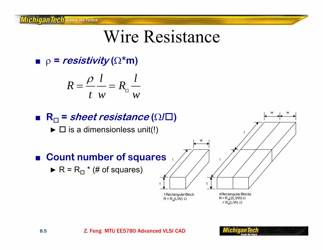
Wire Resistance■ = resistivity (*m)
■ R = sheet resistance (/)► is a dimensionless unit(!)
■ Count number of squares► R = R * (# of squares)
l
w
t
1 Rectangular BlockR = R (L/W)
4 Rectangular BlocksR = R (2L/2W) = R (L/W)
t
l
w w
l
l lR Rt w w
Z. Feng MTU EE5780 Advanced VLSI CAD8.6
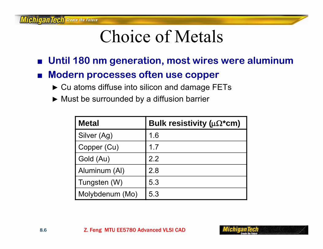
Choice of Metals■ Until 180 nm generation, most wires were aluminum■ Modern processes often use copper
► Cu atoms diffuse into silicon and damage FETs► Must be surrounded by a diffusion barrier
Metal Bulk resistivity (*cm)Silver (Ag) 1.6Copper (Cu) 1.7Gold (Au) 2.2Aluminum (Al) 2.8Tungsten (W) 5.3Molybdenum (Mo) 5.3
Z. Feng MTU EE5780 Advanced VLSI CAD8.7
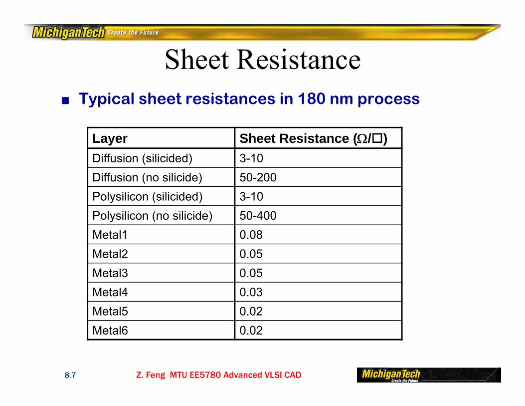
Sheet Resistance■ Typical sheet resistances in 180 nm process
Layer Sheet Resistance (/)Diffusion (silicided) 3-10Diffusion (no silicide) 50-200Polysilicon (silicided) 3-10Polysilicon (no silicide) 50-400Metal1 0.08Metal2 0.05Metal3 0.05Metal4 0.03Metal5 0.02Metal6 0.02
Z. Feng MTU EE5780 Advanced VLSI CAD8.8
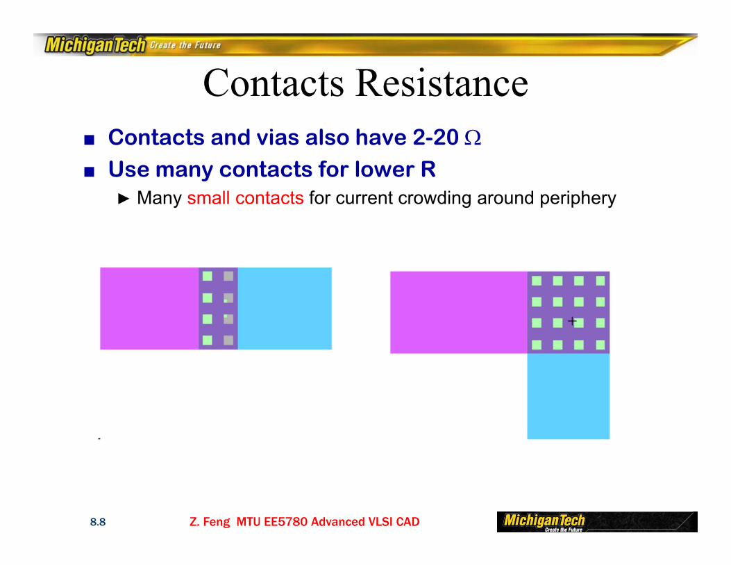
Contacts Resistance■ Contacts and vias also have 2-20 ■ Use many contacts for lower R
► Many small contacts for current crowding around periphery
Z. Feng MTU EE5780 Advanced VLSI CAD8.9
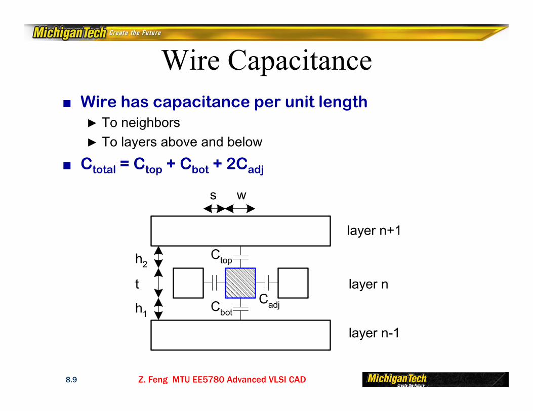
Wire Capacitance■ Wire has capacitance per unit length
► To neighbors► To layers above and below
■ Ctotal = Ctop + Cbot + 2Cadj
layer n+1
layer n
layer n-1
Cadj
Ctop
Cbot
ws
t
h1
h2
Z. Feng MTU EE5780 Advanced VLSI CAD8.10
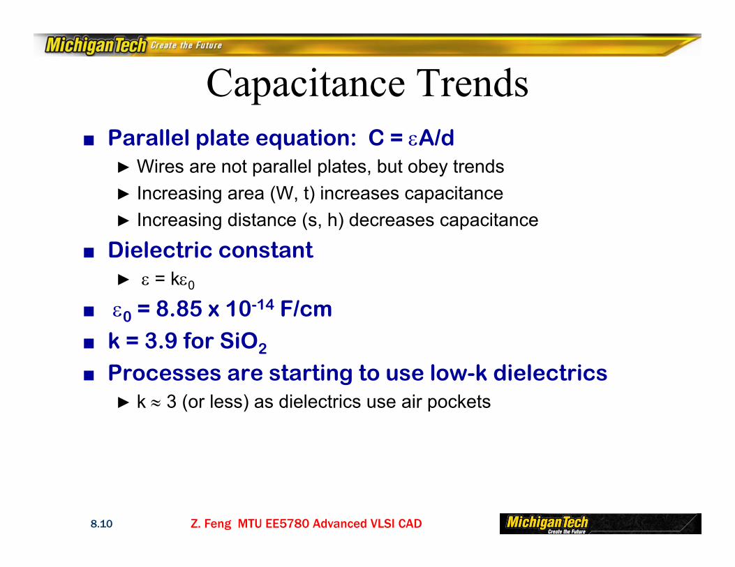
Capacitance Trends■ Parallel plate equation: C = A/d
► Wires are not parallel plates, but obey trends► Increasing area (W, t) increases capacitance► Increasing distance (s, h) decreases capacitance
■ Dielectric constant► = k0
■ 0 = 8.85 x 10⁻¹⁴ F/cm■ k = 3.9 for SiO2
■ Processes are starting to use low-k dielectrics► k 3 (or less) as dielectrics use air pockets
Z. Feng MTU EE5780 Advanced VLSI CAD8.11
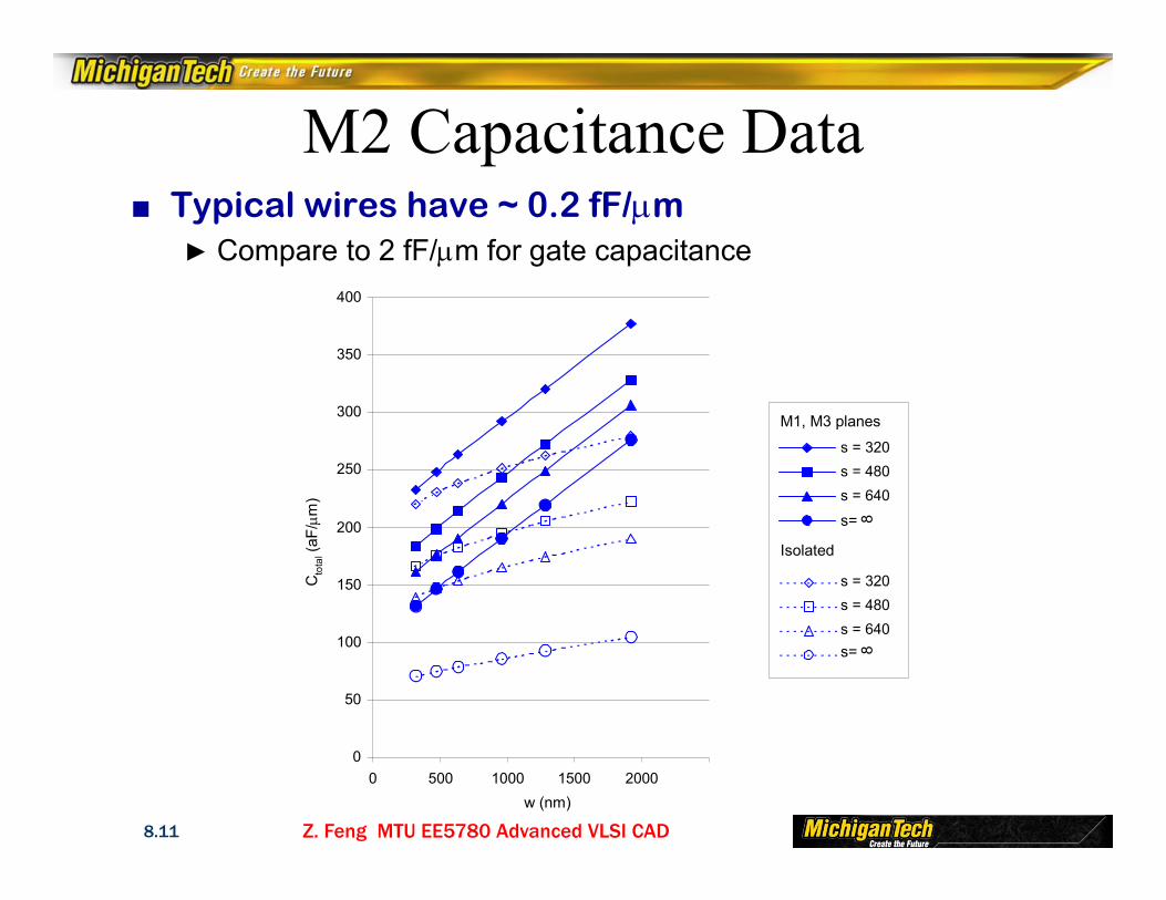
M2 Capacitance Data■ Typical wires have ~ 0.2 fF/m
► Compare to 2 fF/m for gate capacitance
0
50
100
150
200
250
300
350
400
0 500 1000 1500 2000
Cto
tal (
aF/
m)
w (nm)
Isolated
M1, M3 planes
s = 320s = 480s = 640s= 8
s = 320s = 480s = 640
s= 8

Z. Feng MTU EE5780 Advanced VLSI CAD8.12
Diffusion & Polysilicon■ Diffusion capacitance is very high (about 2 fF/m)
► Comparable to gate capacitance► Diffusion also has high resistance► Avoid using diffusion runners for wires!
■ Polysilicon has lower C but high R► Use for transistor gates► Occasionally for very short wires between gates
Z. Feng MTU EE5780 Advanced VLSI CAD8.13
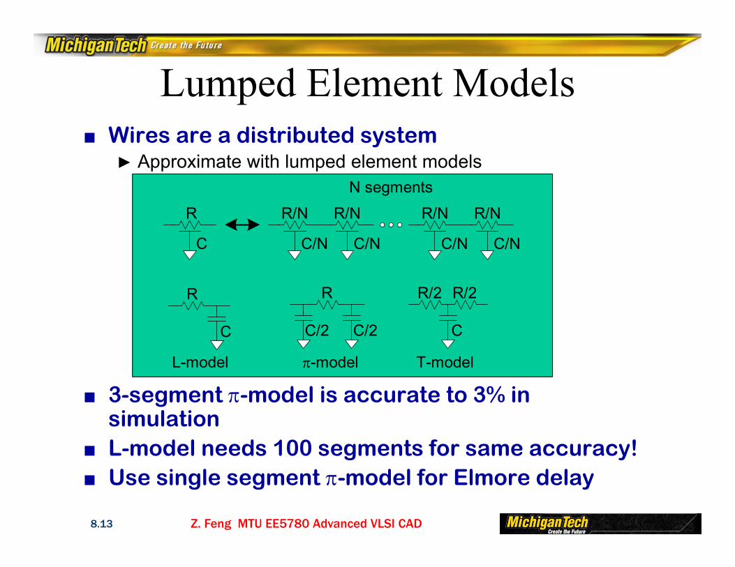
Lumped Element Models■ Wires are a distributed system
► Approximate with lumped element models
■ 3-segment -model is accurate to 3% in simulation
■ L-model needs 100 segments for same accuracy!■ Use single segment -model for Elmore delay
C
R
C/N
R/N
C/N
R/N
C/N
R/N
C/N
R/N
R
C
L-model
R
C/2 C/2
R/2 R/2
C
N segments
-model T-model

Z. Feng MTU EE5780 Advanced VLSI CAD8.14
Crosstalk■ A capacitor does not like to change its voltage
instantaneously.■ A wire has high capacitance to its neighbor.
► When the neighbor switches from 1-> 0 or 0->1, the wire tends to switch too.
► Called capacitive coupling or crosstalk.
■ Crosstalk effects► Noise on nonswitching wires► Increased delay on switching wires
Z. Feng MTU EE5780 Advanced VLSI CAD8.15
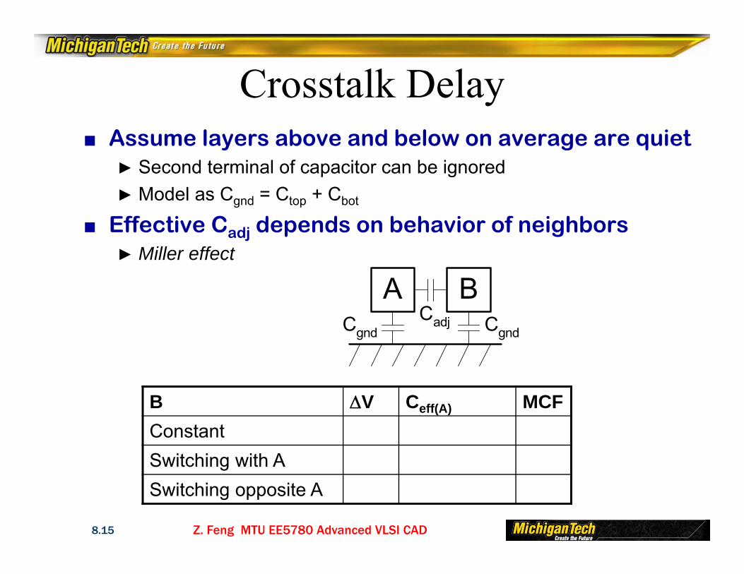
Crosstalk Delay■ Assume layers above and below on average are quiet
► Second terminal of capacitor can be ignored► Model as Cgnd = Ctop + Cbot
■ Effective Cadj depends on behavior of neighbors► Miller effect
A BCadjCgnd Cgnd
B V Ceff(A) MCFConstantSwitching with ASwitching opposite A
Z. Feng MTU EE5780 Advanced VLSI CAD8.16
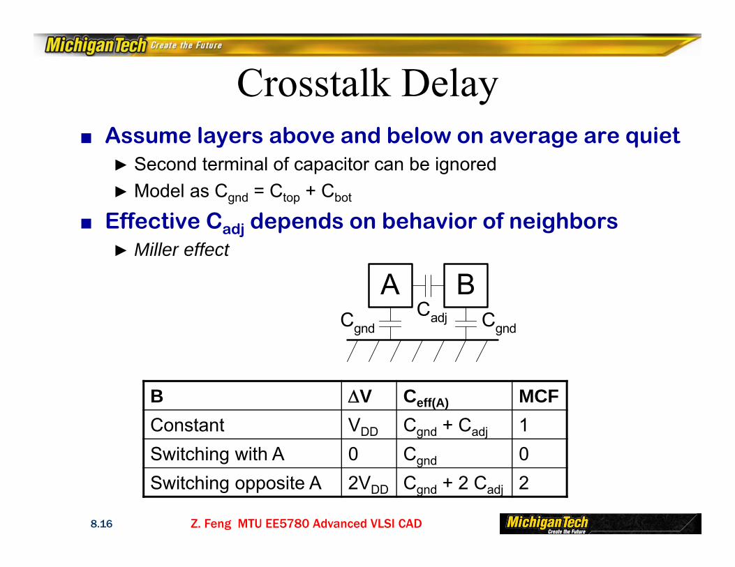
Crosstalk Delay■ Assume layers above and below on average are quiet
► Second terminal of capacitor can be ignored► Model as Cgnd = Ctop + Cbot
■ Effective Cadj depends on behavior of neighbors► Miller effect
A BCadjCgnd Cgnd
B V Ceff(A) MCFConstant VDD Cgnd + Cadj 1Switching with A 0 Cgnd 0Switching opposite A 2VDD Cgnd + 2 Cadj 2

Z. Feng MTU EE5780 Advanced VLSI CAD8.17
Crosstalk Noise■ Crosstalk causes noise on nonswitching wires■ If victim is floating:
► model as capacitive voltage divider
Cadj
Cgnd-v
Aggressor
Victim
Vaggressor
Vvictim
adjvictim aggressor
gnd v adj
CV V
C C
Z. Feng MTU EE5780 Advanced VLSI CAD8.18
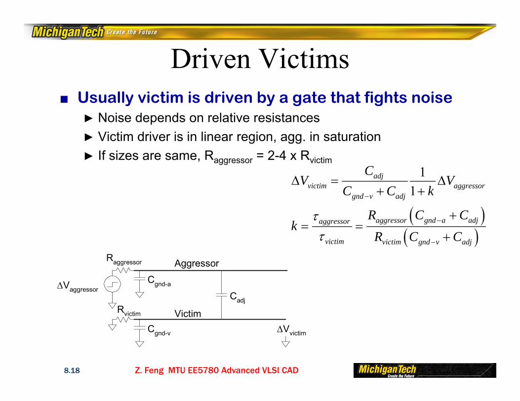
Driven Victims■ Usually victim is driven by a gate that fights noise
► Noise depends on relative resistances► Victim driver is in linear region, agg. in saturation► If sizes are same, Raggressor = 2-4 x Rvictim
11
adjvictim aggressor
gnd v adj
CV V
C C k
aggressor gnd a adjaggressor
victim victim gnd v adj
R C Ck
R C C
Cadj
Cgnd-v
Aggressor
Victim
Vaggressor
Vvictim
Raggressor
Rvictim
Cgnd-a
Z. Feng MTU EE5780 Advanced VLSI CAD8.19
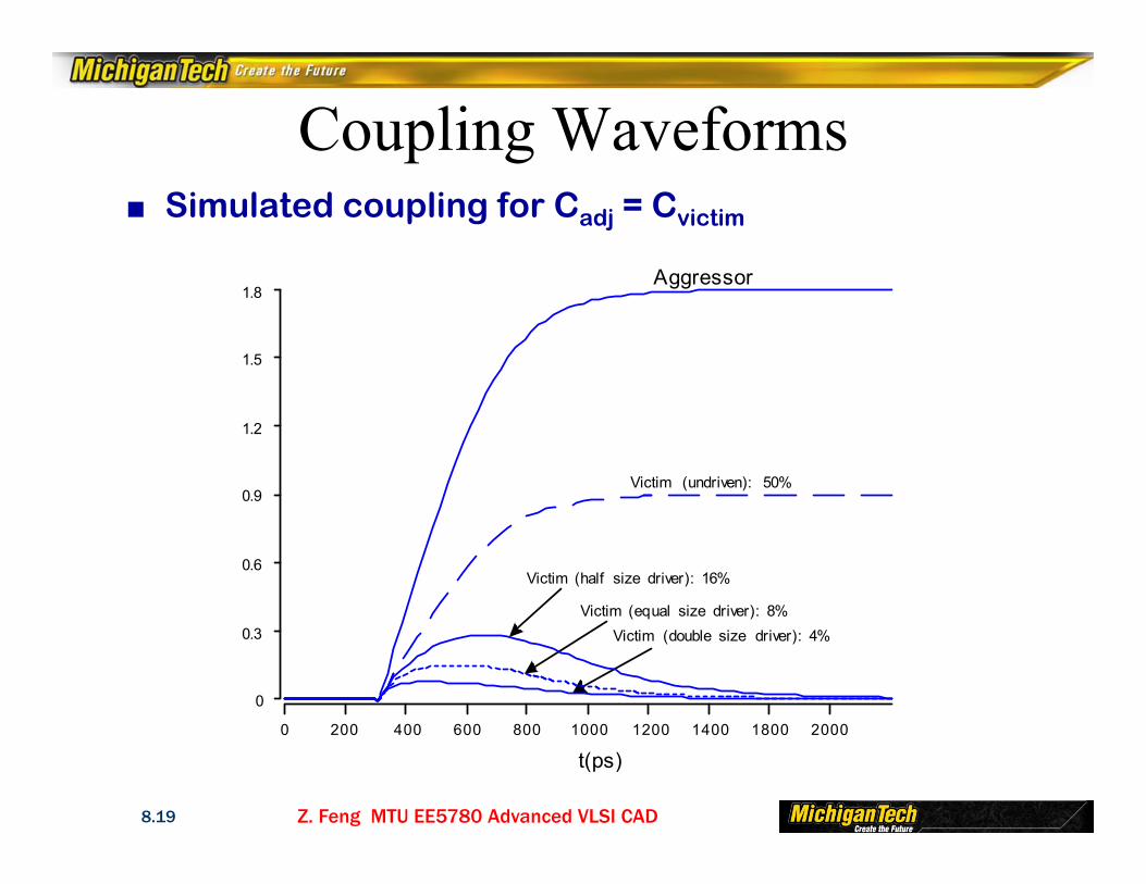
Coupling Waveforms
Aggressor
Victim (undriven): 50%
Victim (half size driver): 16%
Victim (equal size driver): 8%Victim (double size driver): 4%
t (ps)0 200 400 600 800 1000 1200 1400 1800 2000
0
0.3
0.6
0.9
1.2
1.5
1.8
■ Simulated coupling for Cadj = Cvictim
Z. Feng MTU EE5780 Advanced VLSI CAD8.20
Noise Implications■ So what if we have noise?■ If the noise is less than the noise margin, nothing
happens■ Static CMOS logic will eventually settle to correct
output even if disturbed by large noise spikes► But glitches cause extra delay► Also cause extra power from false transitions
■ Dynamic logic never recovers from glitches■ Memories and other sensitive circuits also can
produce the wrong answer
Z. Feng MTU EE5780 Advanced VLSI CAD8.21
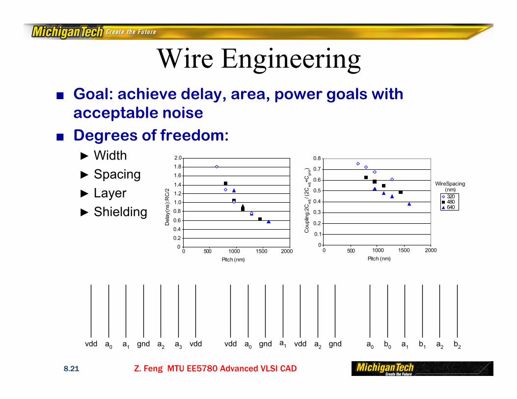
Wire Engineering■ Goal: achieve delay, area, power goals with
acceptable noise■ Degrees of freedom:
► Width ► Spacing► Layer► Shielding
Del
ay (n
s): R
C/2
Wire Spacing(nm)
Cou
plin
g: 2C
adj /
(2C
adj+C
gnd)
00.20.40.6
0.81.01.21.4
1.61.82.0
0 500 1000 1500 20000
0.1
0.2
0.3
0.4
0.5
0.6
0.7
0.8
0 500 1000 1500 2000
320480640
Pitch (nm)Pitch (nm)
vdd a0a1gnd a2vdd b0 a1 a2 b2vdd a0 a1 gnd a2 a3 vdd gnd a0 b1
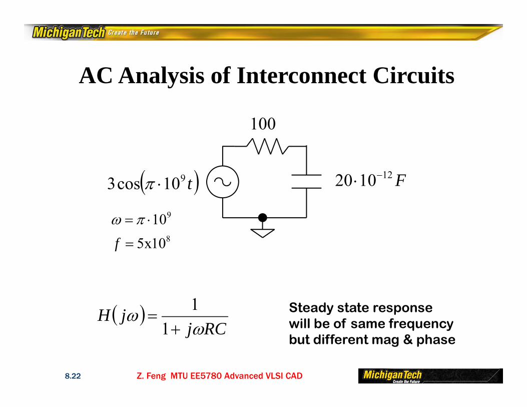
Z. Feng MTU EE5780 Advanced VLSI CAD8.22
Steady state responsewill be of same frequencybut different mag & phase
t910cos3
910 810x5f
100
F121020
RCj
jH
1
1
AC Analysis of Interconnect Circuits
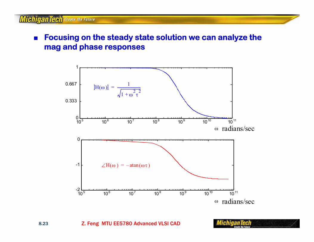
Z. Feng MTU EE5780 Advanced VLSI CAD8.23
H 1
1 2
2+--------------------------=
105 106 107 108 109 1010 10110
0.333
0.667
1
H atan–=
105 106 107 108 109 1010 1011-2
-1
0
radians/sec
radians/sec
■ Focusing on the steady state solution we can analyze the mag and phase responses

Z. Feng MTU EE5780 Advanced VLSI CAD8.24
Formulate nodal equations:
Given a particular value, solve for
)()()( jIjVjY n
Translate complex voltage into magnitude and phase
)( jVn
Problems with C’s as
Bigger problem for L as
0
LjZL LjYL
1
Z. Feng MTU EE5780 Advanced VLSI CAD8.25
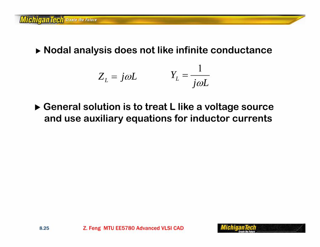
Nodal analysis does not like infinite conductance
General solution is to treat L like a voltage sourceand use auxiliary equations for inductor currents
LjZL LjYL
1

Z. Feng MTU EE5780 Advanced VLSI CAD8.26
Sometimes analog designers prefer poles / zerosinstead of a freq. domain mag. and phase plots
We start by formulating the equations using sinstead of j
)()()( suBsxGsxsC
Z. Feng MTU EE5780 Advanced VLSI CAD8.27
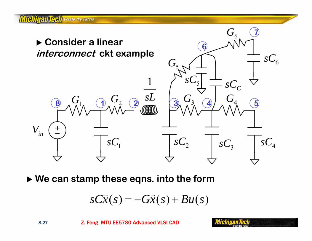
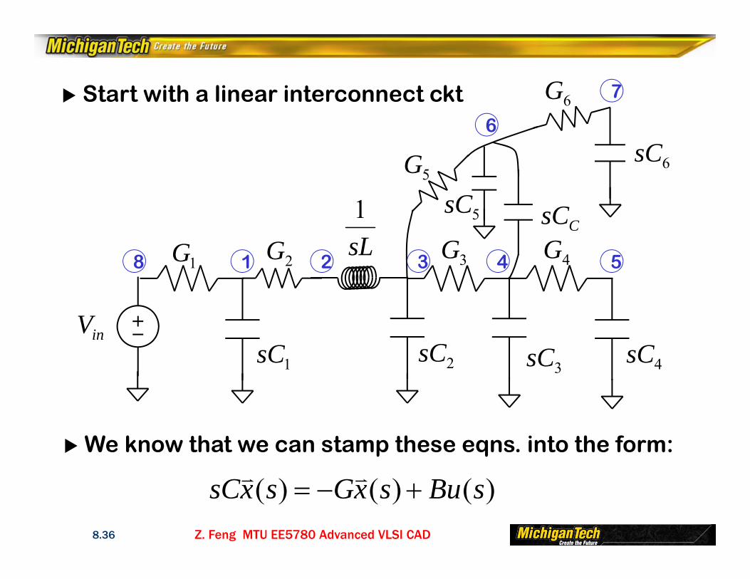
Consider a linear interconnect ckt example
We can stamp these eqns. into the form
)()()( sBusxGsxsC
inV
1G 2G
5G
3G
6G
4G
1sC 2sC3sC 4sC
6sC
CsC5sC
3218
7
6
54sL1
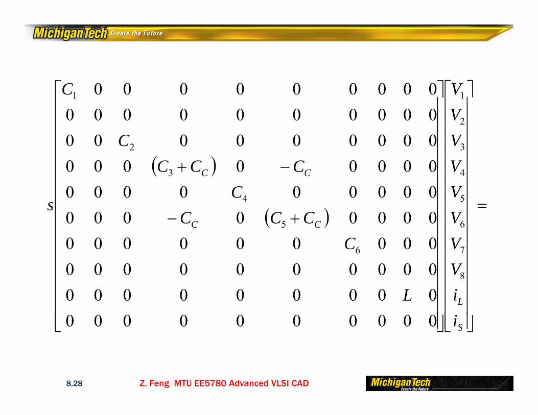
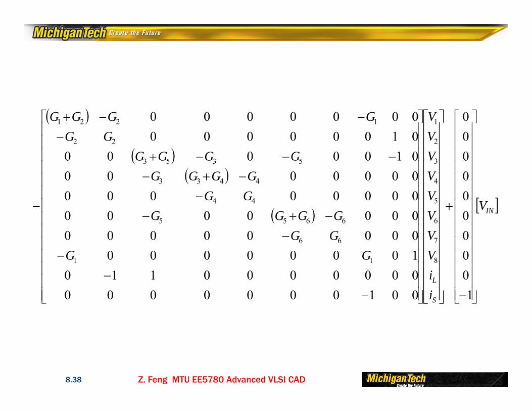
Z. Feng MTU EE5780 Advanced VLSI CAD8.28
S
L
CC
CC
iiVVVVVVVV
L
CCCC
CCCC
C
C
s
8
7
6
5
4
3
2
1
6
5
4
3
2
1
0000000000000000000000000000000000000000000000000000000000000000000000000000000000000000000

Z. Feng MTU EE5780 Advanced VLSI CAD8.29
IN
S
L
V
iiVVVVVVVV
GGGGGGGG
GGGGGG
GGGGGG
GGGG
1000000000
00100000000000000110100000000000000000000000000000000000000100000010000000000000
8
7
6
5
4
3
2
1
11
66
6655
44
4433
5353
22
1221
Z. Feng MTU EE5780 Advanced VLSI CAD8.30
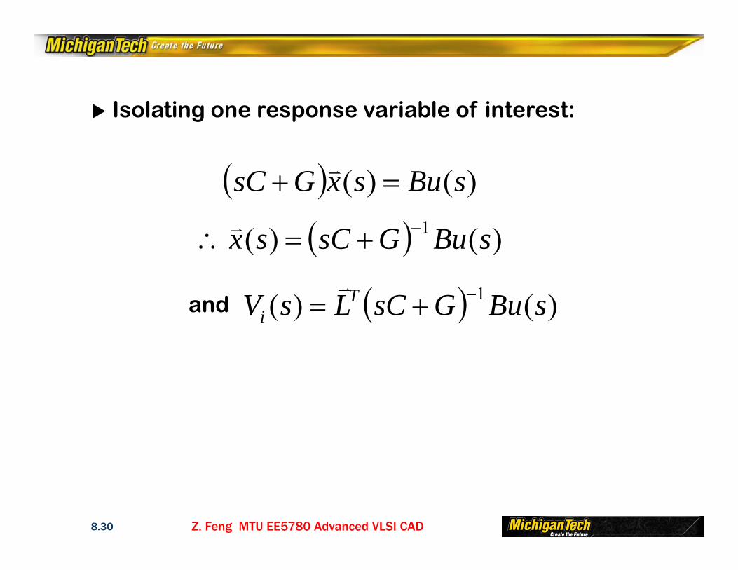
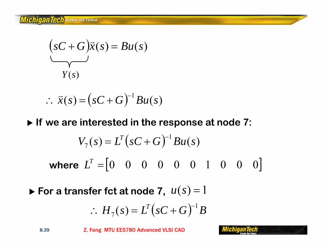
Isolating one response variable of interest:
)()( sBusxGsC
)()( 1 sBuGsCsx
)()( 1 sBuGsCLsV Ti
and
Z. Feng MTU EE5780 Advanced VLSI CAD8.31
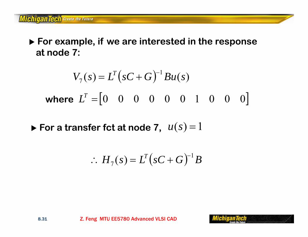
For example, if we are interested in the response at node 7:
)()( 17 sBuGsCLsV T
0001000000TLwhere
For a transfer fct at node 7, 1)( su
BGsCLsH T 17 )(

Z. Feng MTU EE5780 Advanced VLSI CAD8.32
We know from Cramer’s Rule that any node voltagesolution will be of the form:
GsCTsVi
det
det)(
n
m
pspspszszszs
21
21
The roots of are the ckt poles 0det GsC
)()( 1 sBuGsCLsV Ti
Z. Feng MTU EE5780 Advanced VLSI CAD8.33
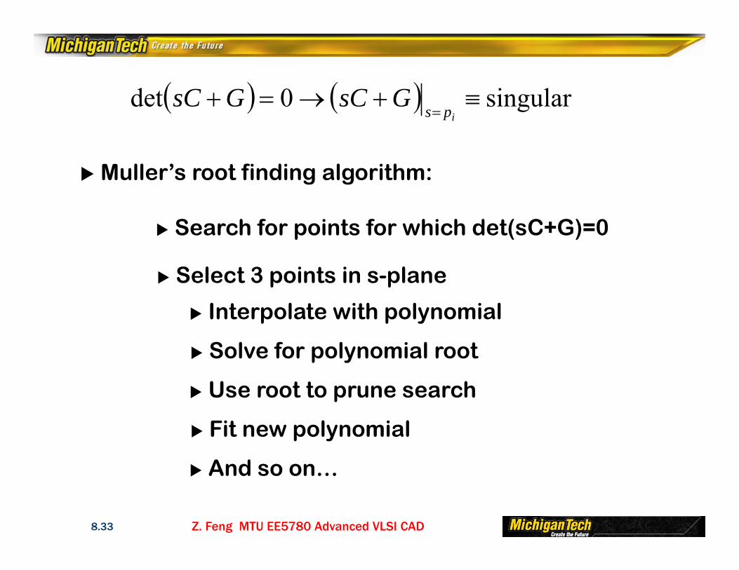
singular0det ips
GsCGsC
Muller’s root finding algorithm:
Search for points for which det(sC+G)=0
Select 3 points in s-plane
Interpolate with polynomial
Solve for polynomial root
Use root to prune search
Fit new polynomial
And so on…

Z. Feng MTU EE5780 Advanced VLSI CAD8.34
How do we test to see if
LU Factor Y
Difficult to find all of the poles in a freq. range reliably
ULY detdetdet Ldet
0sY
We’ll actually show a better way of doing this using model order reduction methods
Z. Feng MTU EE5780 Advanced VLSI CAD8.35
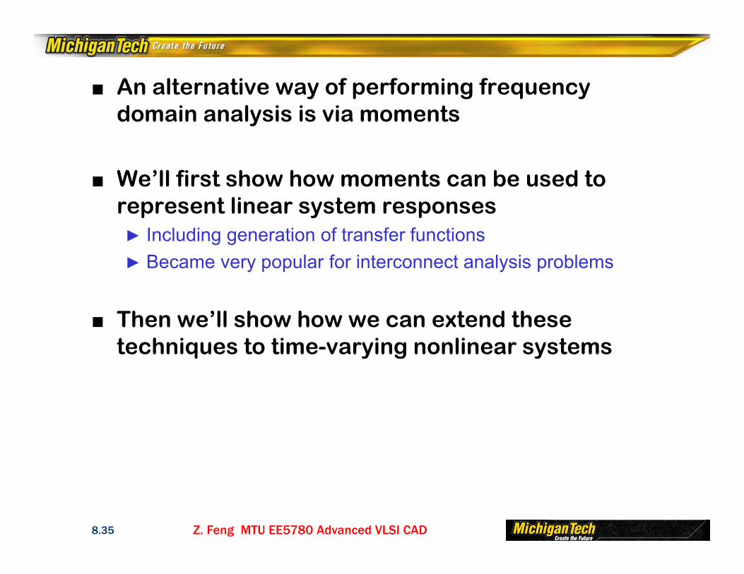
■ An alternative way of performing frequency domain analysis is via moments
■ We’ll first show how moments can be used to represent linear system responses► Including generation of transfer functions► Became very popular for interconnect analysis problems
■ Then we’ll show how we can extend these techniques to time-varying nonlinear systems
Z. Feng MTU EE5780 Advanced VLSI CAD8.36
Start with a linear interconnect ckt
We know that we can stamp these eqns. into the form:
)()()( sBusxGsxsC
inV
1G 2G
5G
3G
6G
4G
1sC 2sC3sC 4sC
6sC
CsC5sC
3218
7
6
54sL1

Z. Feng MTU EE5780 Advanced VLSI CAD8.37
S
L
CC
CC
iiVVVVVVVV
L
CCCC
CCCC
C
C
s
8
7
6
5
4
3
2
1
6
5
4
3
2
1
0000000000000000000000000000000000000000000000000000000000000000000000000000000000000000000
Z. Feng MTU EE5780 Advanced VLSI CAD8.38
IN
S
L
V
iiVVVVVVVV
GGGGGGGG
GGGGGG
GGGGGG
GGGG
1000000000
00100000000000000110100000000000000000000000000000000000000100000010000000000000
8
7
6
5
4
3
2
1
11
66
6655
44
4433
5353
22
1221
Z. Feng MTU EE5780 Advanced VLSI CAD8.39
)()( sBusxGsC
)()( 1 sBuGsCsx )(sY
If we are interested in the response at node 7:
)()( 17 sBuGsCLsV T
0001000000TLwhere
For a transfer fct at node 7, 1)( su
BGsCLsH T 17 )(

Z. Feng MTU EE5780 Advanced VLSI CAD8.40
Generally, we express transfer functions in a similar form:
It’s impractical, however, to calculate transfer functions symbolically for large ckts in either form
Therefore, we instead start with series expansions in s
nmsbsbbsasaasH m
m
nn
10
10
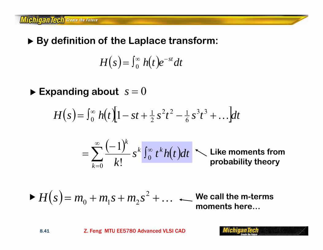
Z. Feng MTU EE5780 Advanced VLSI CAD8.41
By definition of the Laplace transform:
dtethsH st 0
Expanding about 0s
dttstsstthsH 336122
21
0 1
0
0!1
k
kkk
dtthtsk
Like moments fromprobability theory
2210 smsmmsH We call the m-terms
moments here…

Z. Feng MTU EE5780 Advanced VLSI CAD8.42
We can use since can be used to representvalue for s=0
But how many moments do I need to completelyspecify my m-pole system?
2
2101
10
1smsmm
sbsbsasaam
m
nn
10 b 0a
n zeros & m poles
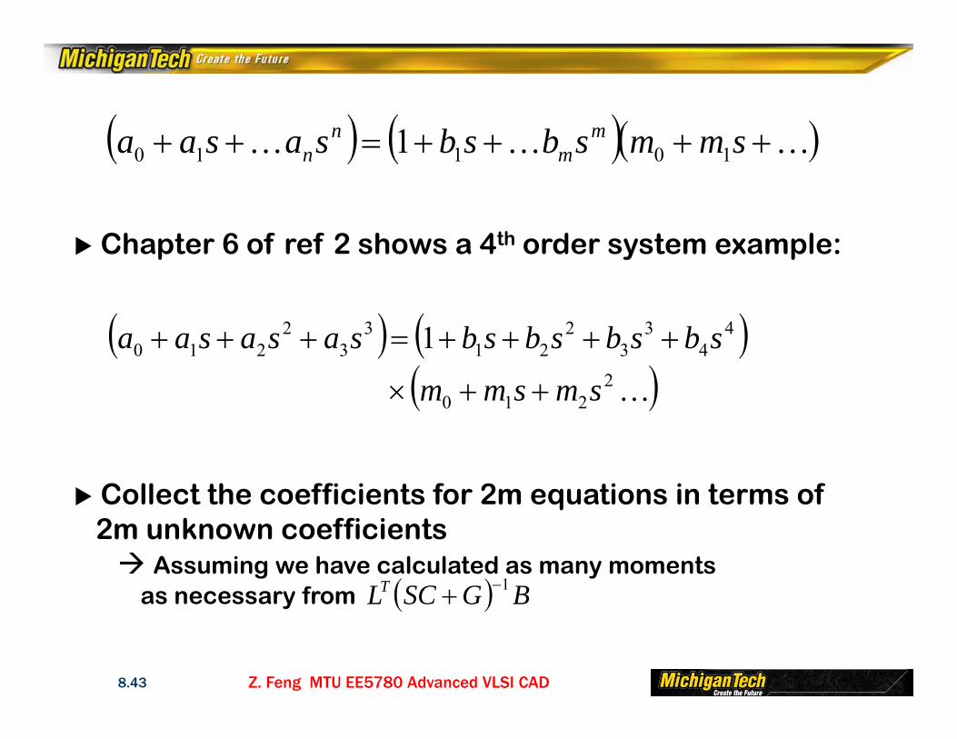
Z. Feng MTU EE5780 Advanced VLSI CAD8.43
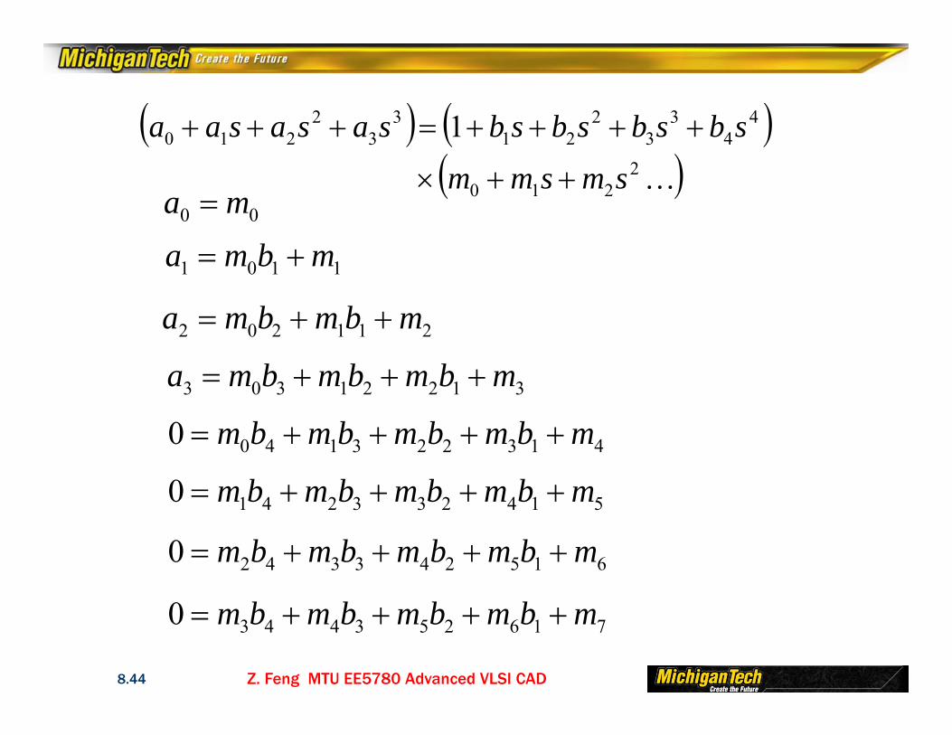
Chapter 6 of ref 2 shows a 4th order system example:
Collect the coefficients for 2m equations in terms of2m unknown coefficients Assuming we have calculated as many moments
as necessary from BGSCLT 1
smmsbsbsasaa mm
nn 10110 1
2
210
44
33
221
33
2210 1
smsmm
sbsbsbsbsasasaa
Z. Feng MTU EE5780 Advanced VLSI CAD8.44
2
210
44
33
221
33
2210 1
smsmm
sbsbsbsbsasasaa
00 ma
1101 mbma
211202 mbmbma
31221303 mbmbmbma
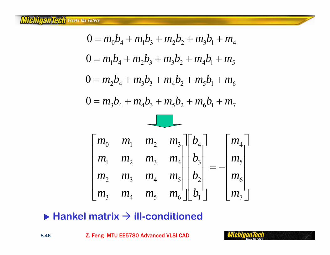
4132231400 mbmbmbmbm
5142332410 mbmbmbmbm
6152433420 mbmbmbmbm
7162534430 mbmbmbmbm
Z. Feng MTU EE5780 Advanced VLSI CAD8.45
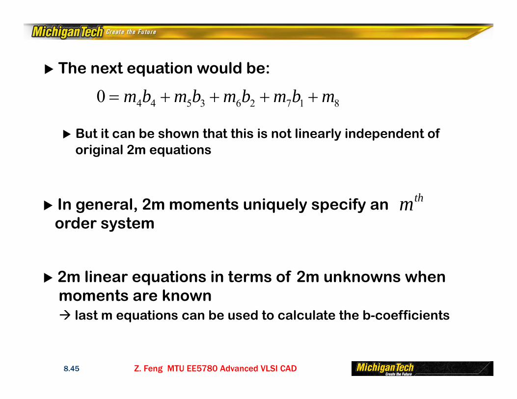
The next equation would be:
8172635440 mbmbmbmbm
But it can be shown that this is not linearly independent of original 2m equations
In general, 2m moments uniquely specify anorder system
2m linear equations in terms of 2m unknowns whenmoments are known last m equations can be used to calculate the b-coefficients
thm
Z. Feng MTU EE5780 Advanced VLSI CAD8.46
4132231400 mbmbmbmbm
5142332410 mbmbmbmbm
6152433420 mbmbmbmbm
7162534430 mbmbmbmbm
7
6
5
4
1
2
3
4
6543
5432
4321
3210
mmmm
bbbb
mmmmmmmmmmmmmmmm
Hankel matrix ill-conditioned
Z. Feng MTU EE5780 Advanced VLSI CAD8.47
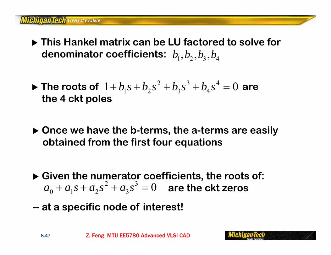
This Hankel matrix can be LU factored to solve fordenominator coefficients:
The roots of arethe 4 ckt poles
4321 ,,, bbbb
01 44
33
221 sbsbsbsb
Once we have the b-terms, the a-terms are easily obtained from the first four equations
Given the numerator coefficients, the roots of:are the ckt zeros
-- at a specific node of interest!
033
2210 sasasaa

Z. Feng MTU EE5780 Advanced VLSI CAD8.48
Poles are the inverse of our time constants Responses are sums of decaying exponentials with
decay rates specified by poles
Zeros specify the residues, -- the amount of “energy” at a particular frequency
tp
ii
iek
ski '

Z. Feng MTU EE5780 Advanced VLSI CAD8.49
All of this assumes that we can calculate moments easily
For an impulse response:
We pre-multiply by to get a response at onenode:
BGsCsx 1)( 1sUsince
2210 sxsxx
TL
...272
71
70
17 smsmmBsCGLsV T
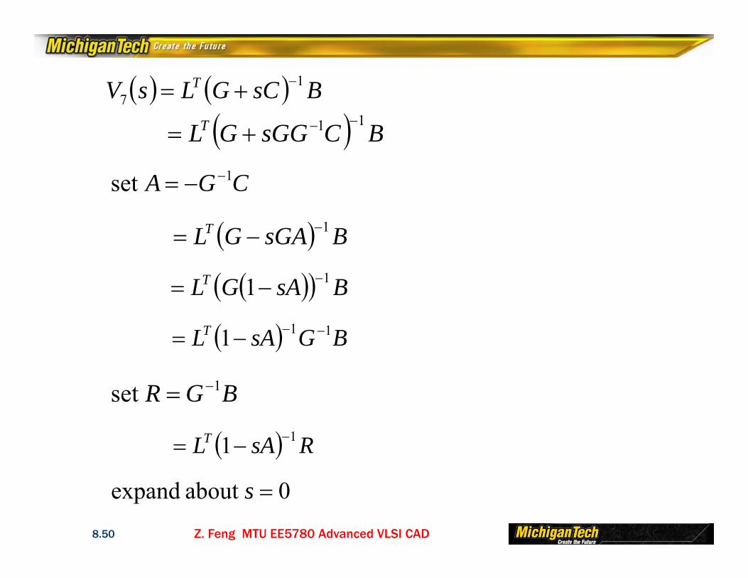
Z. Feng MTU EE5780 Advanced VLSI CAD8.50
BsCGLsV T 17
BCsGGGLT 11
BsGAGLT 1
CGA 1set
BsAGLT 11
BGsALT 111
BGR 1set
RsALT 11
0about expand s

Z. Feng MTU EE5780 Advanced VLSI CAD8.51
RsALsV T 17 1
2
072
2
077 210 ssV
dsdssV
dsdsV ss
07 ssVdsd RAsALT 21
ARLT
072
2
ssVdsd RAsALT 2312
RALT 22
07 sn
n
sVdsd
RALn nT!

Z. Feng MTU EE5780 Advanced VLSI CAD8.52
Clearly we can solve for and andfrom them recursively calculate 2m moments
CGA 1` BGR 1
Then solving the Hankel matrix formulation we canobtain the coefficients for poles’ characteristic eqn
Not a well conditioned matrix problemhowever - - more on this later
Z. Feng MTU EE5780 Advanced VLSI CAD8.53
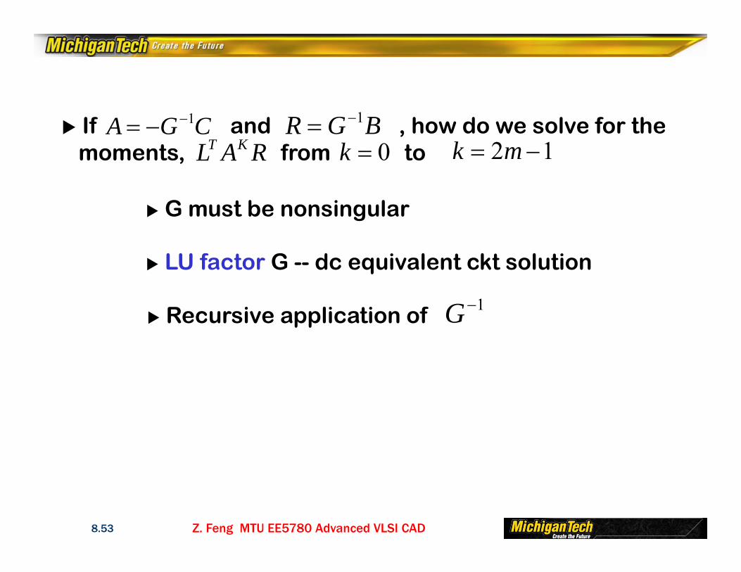
CGA 1 BGR 1 If and , how do we solve for themoments, from toRAL KT 0k 12 mk
G must be nonsingular
LU factor G -- dc equivalent ckt solution
Recursive application of 1G
Z. Feng MTU EE5780 Advanced VLSI CAD8.54
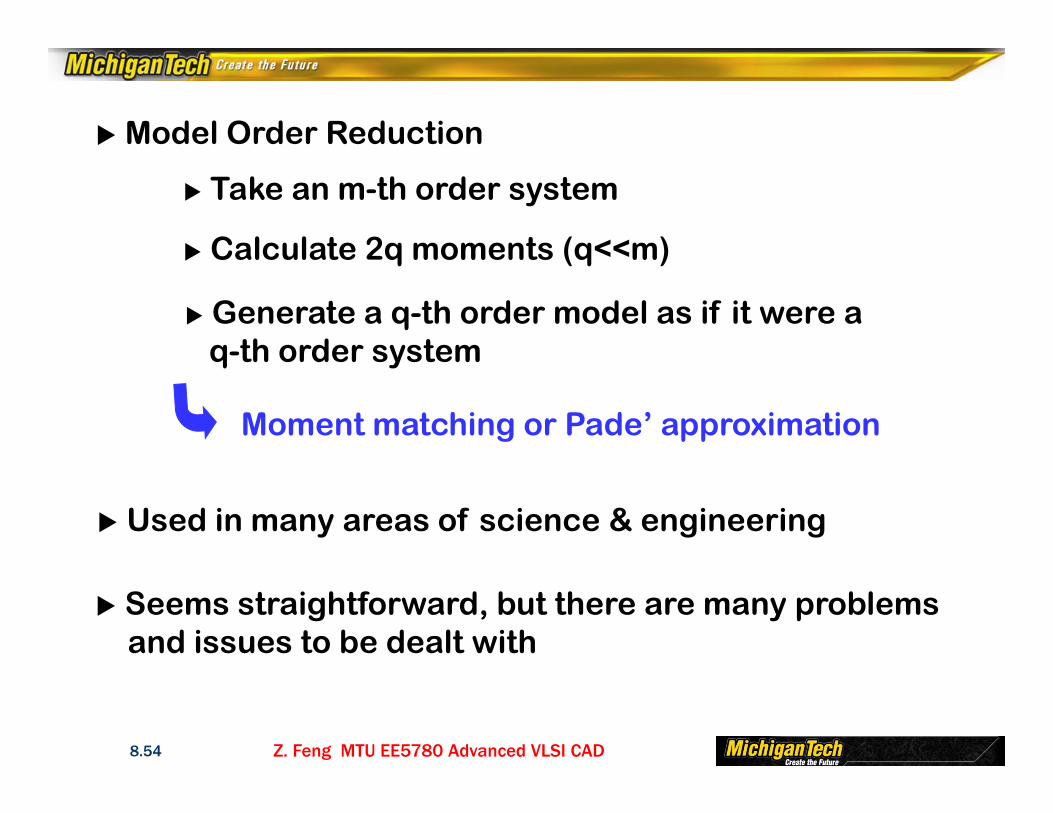
Model Order Reduction
Take an m-th order system
Calculate 2q moments (q<<m)
Generate a q-th order model as if it were aq-th order system
Moment matching or Pade’ approximation
Used in many areas of science & engineering
Seems straightforward, but there are many problemsand issues to be dealt with
Z. Feng MTU EE5780 Advanced VLSI CAD8.55
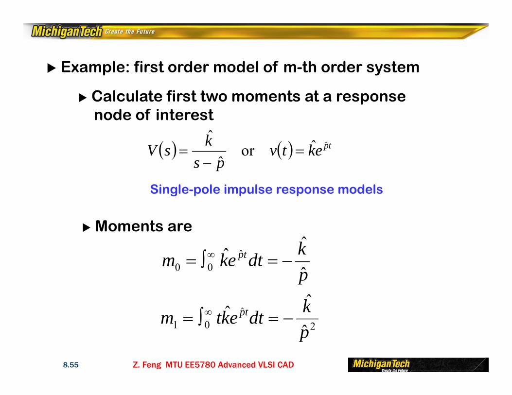
Example: first order model of m-th order system
Calculate first two moments at a responsenode of interest
Moments are
Single-pole impulse response models
tpektvps
ksV ˆˆor ˆ
ˆ
pkdtekm tp
ˆ
ˆˆ ˆ00
2ˆ
01 ˆ
ˆˆpkdtektm tp
Z. Feng MTU EE5780 Advanced VLSI CAD8.56
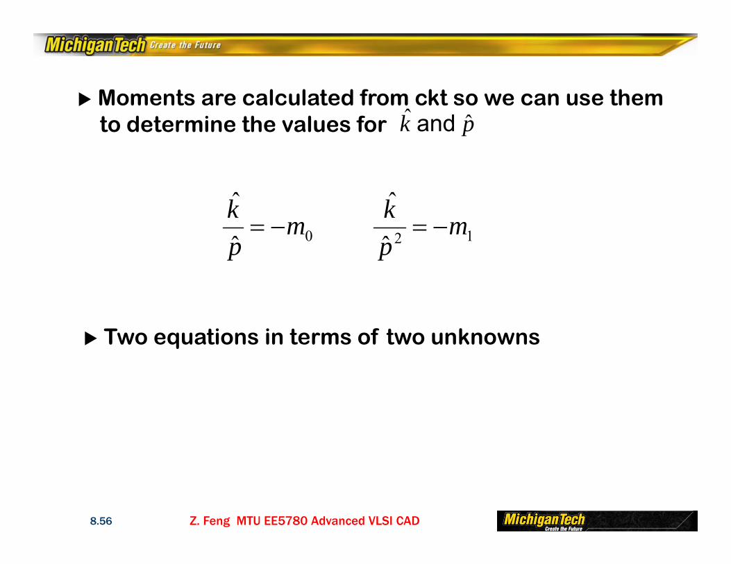
Moments are calculated from ckt so we can use them to determine the values for
0ˆ
ˆm
pk
12ˆ
ˆm
pk
pk ˆˆ and
Two equations in terms of two unknowns
Z. Feng MTU EE5780 Advanced VLSI CAD8.57
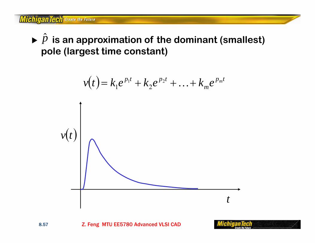
is an approximation of the dominant (smallest)pole (largest time constant)p̂
tpm
tptp mekekektv 2121
tv
t
Z. Feng MTU EE5780 Advanced VLSI CAD8.58
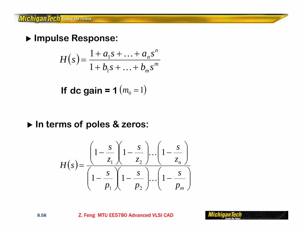
Impulse Response:
If dc gain = 1
In terms of poles & zeros:
mm
nn
sbsbsasasH
1
1
11
m
n
ps
ps
ps
zs
zs
zs
sH111
111
21
21
10 m
Z. Feng MTU EE5780 Advanced VLSI CAD8.59
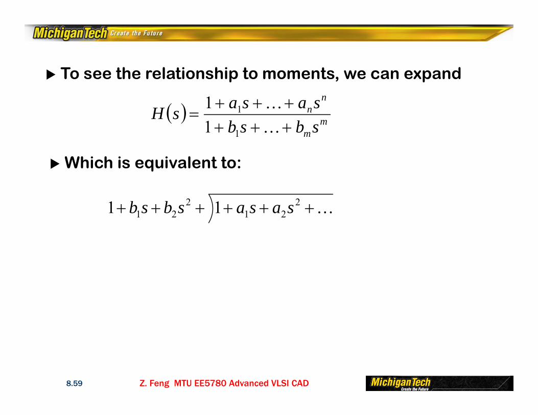
To see the relationship to moments, we can expand
Which is equivalent to:
mm
nn
sbsbsasasH
1
1
11
221
221 11 sasasbsb
Z. Feng MTU EE5780 Advanced VLSI CAD8.60
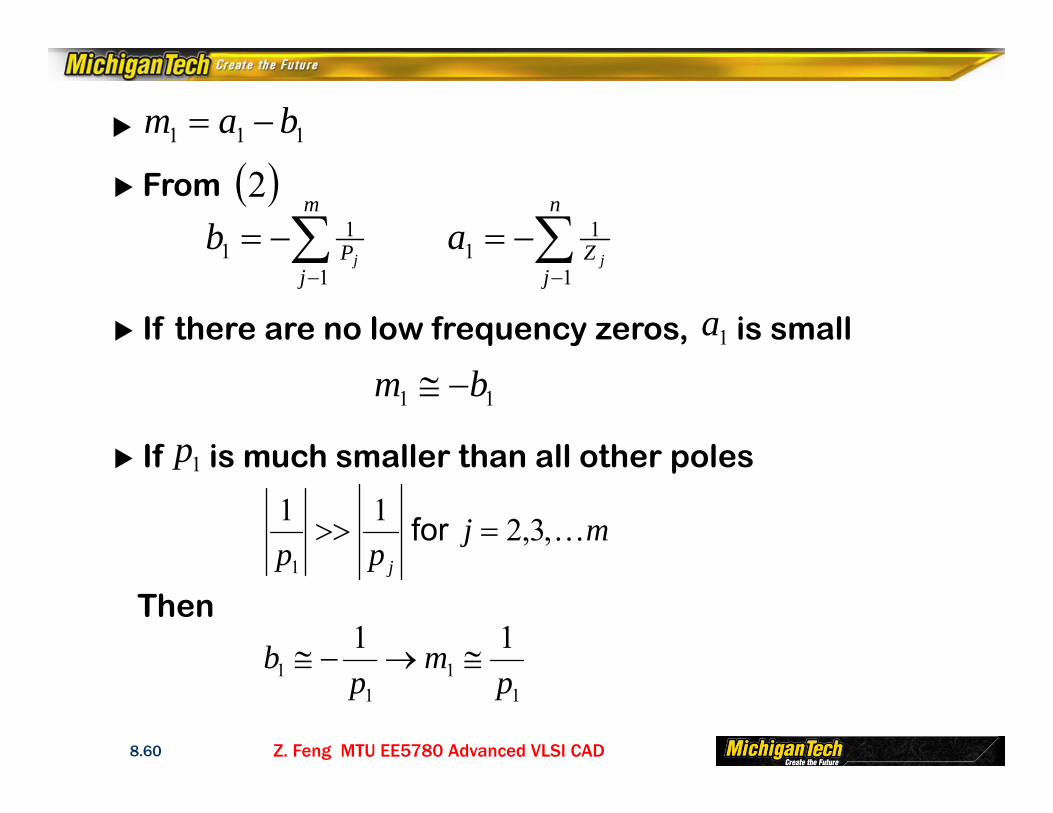
From
If there are no low frequency zeros, is small
If is much smaller than all other poles
111 bam
2
m
jPj
b1
11
n
jZ j
a1
11
11 bm 1a
1p
mjpp j
,3,211
1
for
Then
11
11
11p
mp
b
Z. Feng MTU EE5780 Advanced VLSI CAD8.61
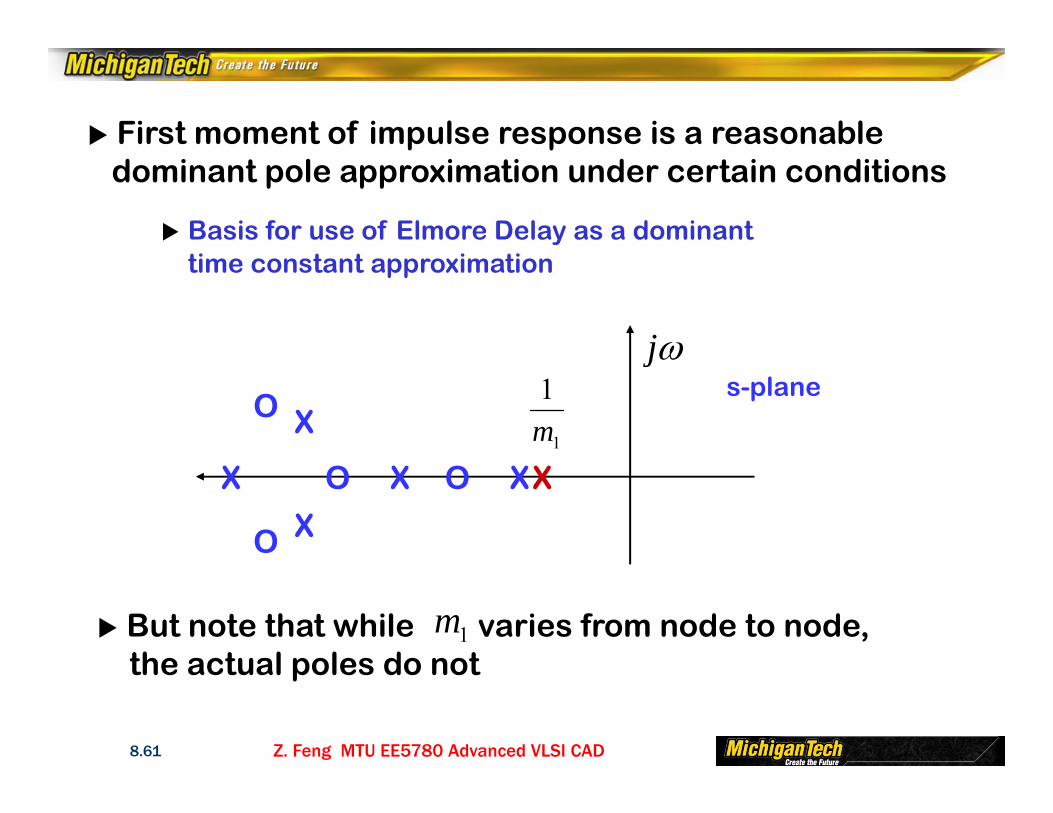
First moment of impulse response is a reasonabledominant pole approximation under certain conditions
Basis for use of Elmore Delay as a dominanttime constant approximation
s-plane
But note that while varies from node to node, the actual poles do not
1m
j
OO
O
O
X
X
X
X XX1
1m
Z. Feng MTU EE5780 Advanced VLSI CAD8.62
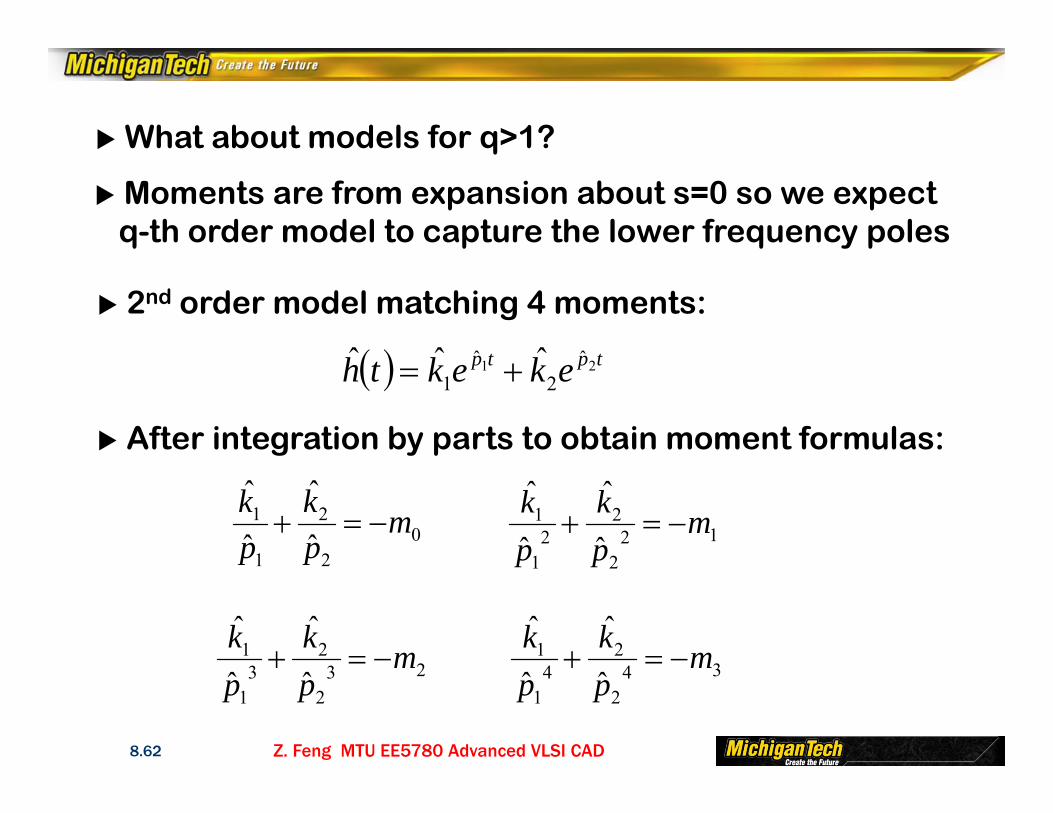
What about models for q>1?
Moments are from expansion about s=0 so we expect q-th order model to capture the lower frequency poles
2nd order model matching 4 moments:
After integration by parts to obtain moment formulas:
tptp ekekth 21 ˆ2
ˆ1
ˆˆˆ
02
2
1
1
ˆ
ˆ
ˆ
ˆm
pk
pk
232
23
1
1
ˆ
ˆ
ˆ
ˆm
pk
pk
122
22
1
1
ˆ
ˆ
ˆ
ˆm
pk
pk
342
24
1
1
ˆ
ˆ
ˆ
ˆm
pk
pk

Z. Feng MTU EE5780 Advanced VLSI CAD8.63
Could solve 4 nonlinear equations in terms of 4 unknown,but a better way is via Hankel matrix equations
Treat this as a 2nd order system:
Solve for b-coefficients, then solve
For the poles
3
2
1
2
21
10
mm
bb
mmmm
01ˆˆ 12
2 pbpb
21 ˆˆ pp and
Z. Feng MTU EE5780 Advanced VLSI CAD8.64
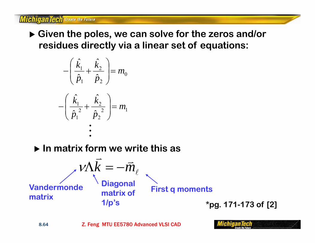
Given the poles, we can solve for the zeros and/orresidues directly via a linear set of equations:
In matrix form we write this as
*pg. 171-173 of [2]
Vandermondematrix
Diagonalmatrix of1/p’s
First q moments
02
2
1
1
ˆ
ˆ
ˆ
ˆm
pk
pk
122
22
1
1
ˆ
ˆ
ˆ
ˆm
pk
pk
mk
Z. Feng MTU EE5780 Advanced VLSI CAD8.65
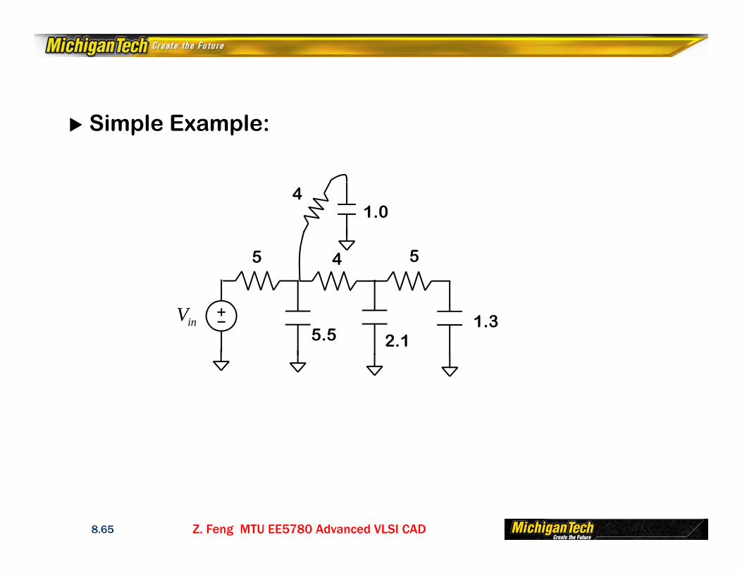
Simple Example:
inV
5
5.5 2.11.3
54
41.0
Z. Feng MTU EE5780 Advanced VLSI CAD8.66
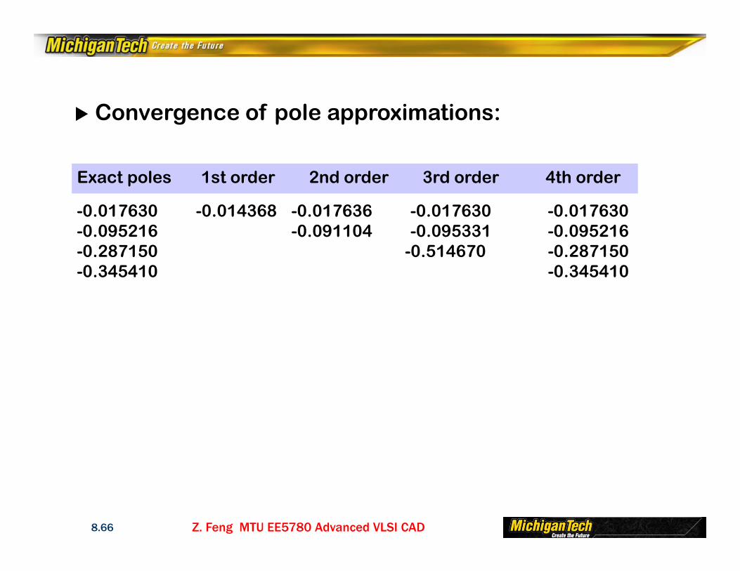
Convergence of pole approximations:
Exact poles 1st order 2nd order 3rd order 4th order
-0.017630 -0.014368 -0.017636 -0.017630 -0.017630-0.095216 -0.091104 -0.095331 -0.095216-0.287150 -0.514670 -0.287150-0.345410 -0.345410
Z. Feng MTU EE5780 Advanced VLSI CAD8.67
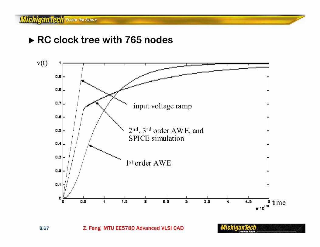
RC clock tree with 765 nodes
input voltage ramp
2nd, 3rd order AWE, andSPICE simulation
1st order AWE
time
v(t)

Z. Feng MTU EE5780 Advanced VLSI CAD8.68
RLC clock tree with 1497 nodes
3rd order AWESPICE simulation
2nd order AWE
1st order AWE
input
time
v(t)
Z. Feng MTU EE5780 Advanced VLSI CAD8.69
In theory we can apply moment matching for anyorder of approximation
But in practice it’s not so simple:
Approximations of stable systems can be unstable
Finite precision problems
Inherent instability of Pade’ approximations


