dynamics of inflation “herding” - brookings … darbha is the executive director and head ......
TRANSCRIPT

DYNAMICS OF INFLATION “HERDING”DECODING INDIA’S INFLATIONARY PROCESS
Gangadhar DarbhaUrjit R. Patel
GLOBAL ECONOMY & DEVELOPMENT
WORKING PAPER 48 | JANUARY 2012
Global Economyand Developmentat BROOKINGS

Global Economyand Developmentat BROOKINGS

Gangadhar Darbha is the executive director and head
of Algorithmic Trading Strategies, Global Markets at
Nomura Structured Finance Services Private Ltd.,
Mumbai.
Urjit R. Patel is a nonresident senior fellow with Global
Economy and Development at Brookings.
Authors’ Note:
We are grateful to Ravi Jaganathan, Rangarajan Sunderam and P. J. Nayak for useful discussions. The views ex-
pressed here are personal and should not be attributed to the authors’ affi liated institutions.
CONTENTS
Abstract . . . . . . . . . . . . . . . . . . . . . . . . . . . . . . . . . . . . . . . . . . . . . . . . . . . . . . . . . . . . . . . . . . . . . . . . . . . . . . .1
Introduction . . . . . . . . . . . . . . . . . . . . . . . . . . . . . . . . . . . . . . . . . . . . . . . . . . . . . . . . . . . . . . . . . . . . . . . . . . 2
Motivation for Investigation . . . . . . . . . . . . . . . . . . . . . . . . . . . . . . . . . . . . . . . . . . . . . . . . . . . . . . . . . . . . . 7
Results: Moments Approach . . . . . . . . . . . . . . . . . . . . . . . . . . . . . . . . . . . . . . . . . . . . . . . . . . . . . . . . . . . . 9
Results: Comovement . . . . . . . . . . . . . . . . . . . . . . . . . . . . . . . . . . . . . . . . . . . . . . . . . . . . . . . . . . . . . . . . . 13
Role of Common Factors . . . . . . . . . . . . . . . . . . . . . . . . . . . . . . . . . . . . . . . . . . . . . . . . . . . . . . . . . . . 15
Number and Importance of Common Factors . . . . . . . . . . . . . . . . . . . . . . . . . . . . . . . . . . . . . . . 15
Does Food and Energy Infl ation Drive Core Sector Infl ation? . . . . . . . . . . . . . . . . . . . . . . . . . .17
Extent and Source of Infl ation Persistence . . . . . . . . . . . . . . . . . . . . . . . . . . . . . . . . . . . . . . . . . .17
Pure Infl ation Gauges (PIGs) as a Measure of Policy (In-) Effectiveness . . . . . . . . . . . . . . . . . . . . . . 24
Methodology for Measuring PIGs . . . . . . . . . . . . . . . . . . . . . . . . . . . . . . . . . . . . . . . . . . . . . . . . . . . . 25
Conclusions . . . . . . . . . . . . . . . . . . . . . . . . . . . . . . . . . . . . . . . . . . . . . . . . . . . . . . . . . . . . . . . . . . . . . . . . . . 28
References . . . . . . . . . . . . . . . . . . . . . . . . . . . . . . . . . . . . . . . . . . . . . . . . . . . . . . . . . . . . . . . . . . . . . . . . . . 29
Appendix: List of Commodity Groups . . . . . . . . . . . . . . . . . . . . . . . . . . . . . . . . . . . . . . . . . . . . . . . . . . . . 31
Endnotes . . . . . . . . . . . . . . . . . . . . . . . . . . . . . . . . . . . . . . . . . . . . . . . . . . . . . . . . . . . . . . . . . . . . . . . . . . . . 33

DYNAMICS OF INFLATION “HERDING”: DECODING INDIA’S INFLATIONARY PROCESS 1
DYNAMICS OF INFLATION “HERDING”DECODING INDIA’S INFLATIONARY PROCESS
Gangadhar DarbhaUrjit R. Patel
ABSTRACT
Compared to immediately preceding years, that is,
its own recent history, India’s infl ation became
unhinged (thereby reversing creditable performance)
from as far back as 2006. The paper puts forward an
empirical framework to analyze the time series and
cross-sectional dynamics of infl ation in India using a
large panel of disaggregated sector prices for the time
period, 1994/95 to 2010/11. This allows us to rigorously
explore issues that have been, at best, loosely posed
in policy debates such as diffusion or comovement
of infl ation across sectors, role of common and idio-
syncratic factors in explaining variation, persistence,
importance of food and energy price changes to the
overall infl ation process, and contrast the recent ex-
perience with the past. We fi nd, inter alia, that the
current period of high infl ation is more cross-section-
ally diffused, and driven by increasingly persistent
common factors in non-food and non-energy sectors
compared to that in the 1990s; this is likely to make it
more diffi cult for anti-infl ationary policy to gain trac-
tion this time round compared to the past. The paper
has also introduced a novel measure of infl ation, viz.,
Pure Infl ation Gauges (PIGs) in the Indian context by
decomposing price movements into those on account
of: (1) aggregate shocks that have equiproportional
effects on all sector prices; (2) aggregated relative
price effects; and (3) sector-specifi c and idiosyncratic
shocks. If PIGs, in conjunction with our other fi ndings,
for example, on persistence had been used as a mea-
sure of underlying (pure) infl ationary pressures, the
monetary authorities may not have been sanguine
regarding the timeliness of initiating anti-infl ationary
policies.

2 GLOBAL ECONOMY AND DEVELOPMENT PROGRAM
INTRODUCTION
From a broad scanning of the Indian economy, it
is not diffi cult to misinterpret Indian economic
managers’ attitude towards inflation, for the most
part, as cynical. Consumer price infl ation (CPI) has
been virtually in double digits for three years and
the wholesale price index (WPI) has accelerated and
stayed stubbornly high.1 Compared to immediately
preceding years, that is, its own recent history, India’s
infl ation became unhinged, thereby reversing credit-
able performance, from as far back as 2006. In the
last two years, among its major comparators India has
the highest rate of consumer infl ation; it is also vola-
tile in relation to its peers in Asia and the BRICs2 (see
Table 1). It would seem that India has decoupled when
it comes to price behavior; therefore assertions that
imported inflation and external developments—like
global excess liquidity—lies at the root of price devel-
opments in India ring hollow.
The paper has been motivated in no small part to of-
fi cial pronouncements seemingly unencumbered by
methodological rigor. There are several grounds for
distrust by citizens regarding policy makers in this
context. Firstly, offi cials have attributed the upswing
in prices (measured by all indices) to food supply con-
straints, and therefore claim they are powerless to
do anything about it. Secondly, they resort to hand
wringing and public communication that essentially
amounts to “we are staring the problem down” as the
common refrain for an inordinately long time; in tan-
dem, rolling “(mental) spreadsheet forecasts”—that
have been optimistic by some distance—were, and still
are, put out at regular intervals to give succor and
hope to the public. Thirdly, a spate of recent state-
ments seems to suggest that the medium-term ob-
jective of around three percent infl ation articulated
by inter alia the Reserve Bank of India (RBI)3 is being
given a quite burial.
Disquieting and, frankly, obvious questions need to
be raised on public policy grounds. A senior (and se-
rious) offi cial earlier this year described six percent
annual infl ation as “comfortable”, and “quiet accept-
able”—comfortable and acceptable to whom? Is the
suspension of long-standing sound, conservative, in-
fl ationary targets temporary, or, is this the new “nor-
mal”? Answers to these questions aside, what is clear
is that persistence of elevated infl ation is agreeable
to some policy makers. The authorities want to take
credit for India’s growth performance but stay blame-
less on the price front—a case of heads I win, tails you
lose! (see Table 2). Is there a reluctance to admit that
the Indian economy has crossed its “speed limit”,
but growth is being prioritized over price stability?
Answers have been scarce.
While high infl ation is being purveyed by some as nec-
essary, or an inevitable synchronicity for the strong
growth performance, it would seem that other im-
portant stakeholders also tasked with navigating and
managing aggregate demand are being driven astray
on infl ation:
“Our inflation emanates from the supply side
more often. If you look at the infl ation basket with
CPIs and WPI, food has 46 to70 percent in the CPI
basket. If on 46 to 70 percent of the basket I have
not much infl uence, how can I deliver on infl ation
target? Which inflation target do we target? We
have one wholesale price index and four consumer
price indices. For a country with 1.2 billion people,
fragmented markets and vast heterogeneity, can
we have a single number representing Nagaland,
Kerala and Orissa at the same time?” (Subbarao
[2010]).
This is an astonishing series of nihilistic statements—
unassisted by evidence or even a hint of scientific
thoroughness—from the central bank head pleading

DYNAMICS OF INFLATION “HERDING”: DECODING INDIA’S INFLATIONARY PROCESS 3
either hopelessness on account of India being a large
and diverse Federal entity, or, a form of muddled
eclecticism. Let us deconstruct the statement. First,
recent infl ation dynamics are being wholly attributed
to narrow sectoral drivers. Prima facie, in combination
with the evolution in core infl ation (a measure exclud-
ing food and petroleum components) it may be con-
strued as seeking to absolve the monetary authority
from pursuing low and stable infl ation as even a pri-
mary—let alone an overriding or dominant—objective
in the hierarchy of macroeconomic goals. Second, it
is impossible to know which price index to target pres-
ently, and presumably in the future, since India will
continue to be geographically diverse and culturally
heterogeneous! Hence, it is not possible to pursue a
useful or credible infl ation objective on which the cen-
tral bank can be assessed. Third, a consensus among
policy makers, both in government and the central
bank, and acceptance by market participants that
stability of infl ation, as measured by the WPI, will be
pursued seems to have been cast aside and degraded
in terms of priority. In other words, an important “fo-
cal point” has been virtually dropped from the central
bank’s price stability lexicon if this speech is anything
to go by.
This is in stark contrast to the awareness (sensitiv-
ity) shown by then Finance Minister’s statements in
Parliament on the subject of inflation in the early
1990s:
Average 1993 - 2002 2003 2004 2005 2006 2007 2008 2009 2010
Proj. 2011
A l l a d va n c e d economies
2.2 1.8 2.0 2.3 2.4 2.2 3.4 0.1 1.6 2.2
Major advanced economies
1.9 1.7 2.0 2.3 2.4 2.2 3.2 -0.1 1.4 2.0
N e w l y i n d u s -trialised Asian economies
3.1 1.5 2.4 2.2 1.6 2.2 4.5 1.3 2.3 3.8
Developing Asia 6.8 2.7 4.1 3.8 4.2 5.4 7.4 3.1 6.0 6.0
Latin America 39.3 10.4 6.6 6.3 5.3 5.4 7.9 6.0 6.0 6.7
Major emerging economies:
India 7.2 3.8 3.8 4.2 6.2 6.4 8.3 10.9 13.2 7.5
China 6.2 1.2 3.9 1.8 1.5 4.8 5.9 -0.7 3.3 5.0
Brazil 103.5 14.8 6.6 6.9 4.2 3.6 5.7 4.9 5.0 6.3
Russia 95.3 13.7 10.9 12.7 9.7 9.0 14.1 11.7 6.9 9.3
South Africa 7.6 5.8 1.4 3.4 4.7 7.1 11.5 7.1 4.3 4.9
Indonesia 13.8 6.8 6.1 10.5 13.1 6.0 9.8 4.8 5.1 7.1
Turkey 72.0 25.3 8.6 8.2 9.6 8.8 10.4 6.3 8.6 5.7
Table 1: Annual Percentage Change in Consumer Prices
Source: IMF [2011].

4 GLOBAL ECONOMY AND DEVELOPMENT PROGRAM
“The people of India have to face double digit infl a-
tion, which hurts most the poorer sections of our so-
ciety. Infl ation hurts everybody, more so the poorer
segments of our population whose incomes are not
indexed.” (Government of India (GoI) [1991]).
“The Government will remain fully vigilant on the
prices front and will use the Public Distribution
System to counter infl ation and in particular to pro-
tect the poorer sections of the population from high
prices and shortages.” (GoI [1992]).
•
•
“Inflationary expectations have not yet been
purged from the system and infl ationary pressure
could easily build up again if fi scal discipline is re-
laxed.” (GoI [1993]).
Obviously there is no confusion about infl ation met-
rics and motivation for price stability as a national
policy goal by India’s most admired Finance Minister.
Therefore, taken together, the above enunciations
raise the obvious question of whether political or pol-
•
Overall fi scal defi cit (% of
GDP)Seignorage (% of GDP) M3 growth (%)
Interest on central govt. dated securi-
ties (%)Headline (WPI infl ation) (%)
Gdp growth rate (%)
1994/95 9.7 3.0 19.8 11.90 12.6 6.4
1995/96 8.3 2.1 15.6 13.75 8.0 7.3
1996/97 8.4 0.4 16.2 13.69 4.6 8.0
1997/98 9.4 1.7 17.0 12.01 4.4 4.3
1998/99 11.4 1.9 19.8 11.86 5.9 6.7
1999/00 11.2 1.1 17.2 11.77 3.3 6.4
2000/01 10.6 1.1 15.9 10.95 7.2 4.4
2001/02 11.0 1.5 16.0 9.44 3.6 5.8
2002/03 9.8 1.3 16.1 7.34 3.4 3.8
2003/04 9.8 2.4 13.0 5.71 5.5 8.5
2004/05 8.3 1.6 14.0 6.11 6.5 7.5
2005/06 7.9 2.2 15.4 7.34 4.4 9.5
2006/07 6.1 3.2 20.5 7.89 5.4 9.6
2007/08 4.9 4.4 22.1 8.12 4.8 9.3
2008/09 10.5 1.1 20.5 7.69 8.3 6.8
2009/10 11.0 2.6 19.1 7.23 3.8 8.0
2010/11 9.5 2.8 16.0 NA 8.9 8.6
Table 2: Fiscal-Financial-Monetary Indicators, 1994/95 to 2010/11
DYNAMICS OF INFLATION “HERDING”: DECODING INDIA’S INFLATIONARY PROCESS 5
ity preferences have changed regarding tolerable and
acceptable levels of infl ation.
It could be that policymakers have not been remiss in
“wait and watch,” founded on diagnosing the recent
bout of infl ation as narrowly based, that is, catalyzed
by specifi c sectoral causes and shocks which will re-
verse themselves. Ipso facto, headline infl ation will
decline, in some ways, of its own accord (sans timely
activist policy). Was the expectation that infl ation in
specifi c sectors would stay contained and not trans-
mit or diffuse through into other sectors? The con-
verse has transpired which has pushed up core sector
inflation and engendered expectations of higher
generalized inflation. Assertions apart, convincing
evidence has not been forthcoming. It was hoped that
drivers of the extant spell of infl ation were unlikely to
continue, which does not appear to be based on any
known analysis.
Alternatively, it may be argued that policymakers
deliberately chose to “fall behind the curve” in formu-
lating, communicating and implementing requisite/
optimal decisions. Were errors of judgment made in
accommodating individual price level shocks, or, im-
pulses emanating from the supply side? Furthermore,
did the government’s loose fi scal-fi nancial-monetary
stance evident in recent years impart pressure to keep
government borrowing rates low or negative in real
terms (see Table 2)?4 In this context, pursuit of quanti-
tative easing (seignorage) would be an important fac-
tor, otherwise why pursue this course of action after
a self imposed hiatus, and against the spirit—if not the
word—of the September 1994 agreement between the
central bank and the Ministry of Finance.5
There is an established tradition for studying infl a-
tion in India. Much of this entails modeling macroeco-
nomic interactions between output, prices and money,
deploying variants around a vector autoregression
framework using quarterly data (Bhattacharya and
Kathuria [1995], Roy and Darbha [2000], and Patra
and Ray [2010], among others). The work has often
been against the background of a lively debate be-
tween two schools of thought, viz., Monetarism and
Structuralism, where differences are primarily due
to variation in the underlying output-price determi-
nation mechanisms emanating from differences in
perceived structural characteristics of the economy
(Balakrishnan [1991]).6
While we don’t comment on—let alone delve into—the
merits or demerits of the WPI, our choice price series
is informed by the following:7
Infl ation measured by the WPI is used by the RBI to
keep track of price developments. In addition, over
the past two decades, indications in offi cial docu-
ments regarding comfort bands/zones, projections,
estimates etc. have been in terms of this index.
In terms of disaggregation (that is, number of com-
modities) it is the most comprehensive among indi-
ces available.
Most importantly, the paper puts forward a formal
scaffolding to understand infl ation dynamics irre-
spective of price data series. If the RBI uses the WPI
to inform its conduct of monetary policy—which it
does—then, we feel, it should bring to bear on the
WPI the operational framework that we put for-
ward.
The paper attempts to comprehensively probe chang-
ing aspects of India’s inflation dynamics informed,
guided and disciplined by deploying diverse estima-
tion techniques and specifi cations, some of which are
atypical. While we are motivated by recent develop-
ments in aggregate infl ation we use disaggregated
price data, thereby preserving the statistical power
of a large panel data set. Although there is a lot of
•
•
•
6 GLOBAL ECONOMY AND DEVELOPMENT PROGRAM
discussion on sector prices and its relationship with
aggregate developments, comprehensive analysis
that pools information in large dimensional panels
available for India are conspicuous by their absence.
(Mishra and Roy [2011] is a recent exception but their
focus is on accounting for importance of food price
inflation.) After all, depending on viewpoints and
context, investigation of both aggregate and disag-
gregated multi-sector price outcomes should be infor-
mative for macroeconomists. For instance, it is useful
to rigorously gauge how broad based sector infl ation
is for a given overall headline measure. While policy
makers have tools to infl uence overall infl ation, the
magnitude of the challenge is, in no small part, de-
termined by the extent to which infl ationary impulses
(dynamics) have played out, or permeated, within and
across sectors on account of standard input-output
price transmissions. The more broad based infl ation
is—especially when converging to a high headline rate,
say—the more stubborn it is likely to be, that is, less
amenable to amelioration with minimal output losses.
This perspective is at the heart of taming generalized
inflationary expectations, especially in the context
that India fi nds itself in at present: high infl ation in
comparison to its own recent past and in relation to
its peers.
Overall, we allow the infl ation data per se to “do the
talking”. Against the background of long standing con-
ceptual work in macroeconomics, fi nance-theoretic
approaches to empirically investigate “convergence/
herding” in price movements and debates within the
country, the paper applies eclectic methodologies to
investigate the behavior of and the interrelationships
between aggregate infl ation and disaggregated core
sectoral inflation over time (the latter is obtained
after stripping away direct and indirect impacts of
food and energy price movements). The emphasis on
dynamics is informed by: (i) the unexceptionable ob-
servation that the Indian economy is undergoing large
changes since the 1990s; and (ii) public comments by
decision makers seem to convey that policy objectives
are changing, or at least being re-examined, in recent
times.
The plan for the rest of the paper is as follows. In
section two, we briefl y review some relevant concep-
tual work on infl ation that forms a backdrop to our
empirical investigations in subsequent sections. It is
natural that we begin by investigating the time-se-
ries evolution of cross-sectional density functions of
sector price changes, a so-called moments approach
(Section Three). In light of the positive and increasing
skewness observed in recent years, we examine the
possibility of rising comovement among sector infl a-
tion rates by analyzing (i) “response coeffi cients” of
sector infl ation to movements in aggregate infl ation;
and (ii) the number and the amount of variation ex-
plained by common dynamic factors (section four).8
Following on, in the same section we estimate the per-
sistence of common factors vis-à-vis sector specifi c
factors for establishing whether or not incessant sec-
tor infl uences are holding sway in adversely impacting
broader (headline) measures of infl ation, say, through
an input cost and/or wage-good price spiral, rather
than broad macro infl uences, say, demand manage-
ment and expectations driven. In section fi ve, we put
forward a novel measure of infl ation, Pure Infl ation
Gauges (PIGs), in the Indian context. The dynamic
common factor estimation exercise introduced in the
previous section allows us to decompose sector price
movements into those on account of (i) aggregate
shocks that are common and have equiproportional
effects; (ii) aggregated relative price effects; and (iii)
idiosyncratic sector specifi c factors (Reis and Watson
[2010]). Section six concludes the paper, followed by
all tables and fi gures.
DYNAMICS OF INFLATION “HERDING”: DECODING INDIA’S INFLATIONARY PROCESS 7
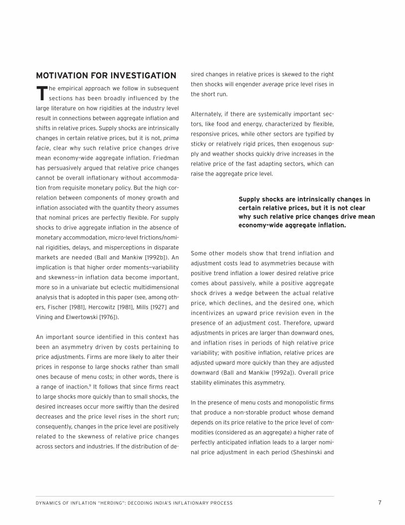
MOTIVATION FOR INVESTIGATION
The empirical approach we follow in subsequent
sections has been broadly influenced by the
large literature on how rigidities at the industry level
result in connections between aggregate infl ation and
shifts in relative prices. Supply shocks are intrinsically
changes in certain relative prices, but it is not, prima
facie, clear why such relative price changes drive
mean economy-wide aggregate inflation. Friedman
has persuasively argued that relative price changes
cannot be overall infl ationary without accommoda-
tion from requisite monetary policy. But the high cor-
relation between components of money growth and
infl ation associated with the quantity theory assumes
that nominal prices are perfectly fl exible. For supply
shocks to drive aggregate infl ation in the absence of
monetary accommodation, micro-level frictions/nomi-
nal rigidities, delays, and misperceptions in disparate
markets are needed (Ball and Mankiw [1992b]). An
implication is that higher order moments—variability
and skewness—in inflation data become important,
more so in a univariate but eclectic multidimensional
analysis that is adopted in this paper (see, among oth-
ers, Fischer [1981], Hercowitz [1981], Mills [1927] and
Vining and Elwertowski [1976]).
An important source identified in this context has
been an asymmetry driven by costs pertaining to
price adjustments. Firms are more likely to alter their
prices in response to large shocks rather than small
ones because of menu costs; in other words, there is
a range of inaction.9 It follows that since fi rms react
to large shocks more quickly than to small shocks, the
desired increases occur more swiftly than the desired
decreases and the price level rises in the short run;
consequently, changes in the price level are positively
related to the skewness of relative price changes
across sectors and industries. If the distribution of de-
sired changes in relative prices is skewed to the right
then shocks will engender average price level rises in
the short run.
Alternately, if there are systemically important sec-
tors, like food and energy, characterized by fl exible,
responsive prices, while other sectors are typifi ed by
sticky or relatively rigid prices, then exogenous sup-
ply and weather shocks quickly drive increases in the
relative price of the fast adapting sectors, which can
raise the aggregate price level.
Some other models show that trend inflation and
adjustment costs lead to asymmetries because with
positive trend infl ation a lower desired relative price
comes about passively, while a positive aggregate
shock drives a wedge between the actual relative
price, which declines, and the desired one, which
incentivizes an upward price revision even in the
presence of an adjustment cost. Therefore, upward
adjustments in prices are larger than downward ones,
and inflation rises in periods of high relative price
variability; with positive infl ation, relative prices are
adjusted upward more quickly than they are adjusted
downward (Ball and Mankiw [1992a]). Overall price
stability eliminates this asymmetry.
In the presence of menu costs and monopolistic fi rms
that produce a non-storable product whose demand
depends on its price relative to the price level of com-
modities (considered as an aggregate) a higher rate of
perfectly anticipated infl ation leads to a larger nomi-
nal price adjustment in each period (Sheshinski and
Supply shocks are intrinsically changes in certain relative prices, but it is not clear why such relative price changes drive mean economy-wide aggregate infl ation.

8 GLOBAL ECONOMY AND DEVELOPMENT PROGRAM
Weiss [1977]). A natural corollary is that expectation
of higher trend infl ation is likely to accentuate skew-
ness of the cross-sectional distribution and increased
comovement of sector infl ation rates in this general
class of forward looking models.
To investigate whether such patterns are corrobo-
rated by the data, we analyze, in what follows, the
time series evolution of cross-sectional densities of
sector infl ation rates and determine whether there is
a perceptible change in the cross-sectional moments
in recent times.

DYNAMICS OF INFLATION “HERDING”: DECODING INDIA’S INFLATIONARY PROCESS 9
RESULTS: MOMENTS APPROACH
To give an initial sense of cross-sectional patterns,
for the years 1994/95 to 2010/11, we investigate
the time series evolution of Kernel Density Function
(KDF) plots of the following:10 11
Annual infl ation for 54 groups, across 360 individ-
ual commodities, comprising the core sectors (non-
food, non-energy) of the wholesale price index (core
sector-WPI), πcit.
12
Residuals from the following regression for core
commodity groups:
πcit = α
i +
i=0Σl
ϕt-i
food infl ationt-i
+ i=0Σl
γt-i
energy
infl ationt-i
+ ε cit (1)
where l = 0, 1, 2, ….
iii. Annual infl ation for 63 groups, across 520 individ-
ual commodities, comprising the entire WPI (WPI-
all), πit.
Much of our analysis is concentrated on variables (i)
and (ii). For the latter, the motivation is to expunge,
as far as possible, effects of food and energy on core
components of the WPI; that is, eliminate higher
order effects of food and energy emanating from
input-output considerations and supply shocks lead-
ing to wage-price linkages through wage-good prices.
Estimated residuals,ε cit, in (1) are denoted CO-RES
it, for
core sector residuals, or, akin to controlled core sector
infl ation.13
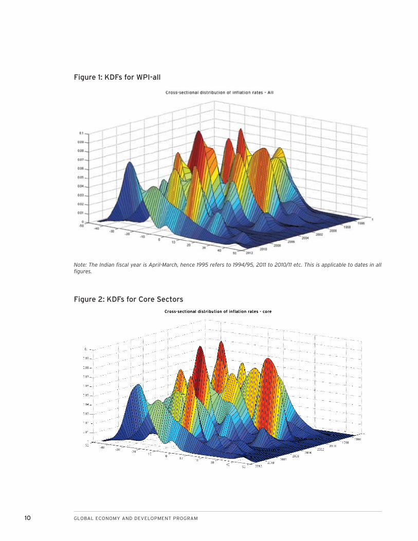
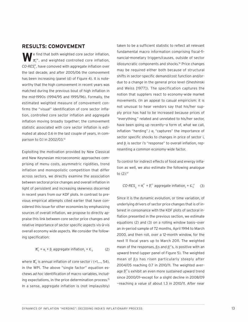
In Figures 1-3 it is noticeable that there has been an
increased asymmetry in the cross-sectional density of
infl ation rates during recent years compared to earlier
years. This fi nding is similar for πit,
πc
it and CO-RES
it,
indicating possible upward mobility of core sector in-
fl ation rates, even after controlling for the indirect ef-
fects emanating from shocks to the food and energy
sectors.
i.
ii.
For a snapshot of unconditional changes in the distri-
bution, the fi rst three panels in Figure 4 summarize
the evolution of annual πit,
πc
it and CO-RES
it. Panels
(a), (b) and (c) are plots of annual weighted mo-
ments—mean, variance and skewness respectively—
for the most recent 17 years. All three moments
exhibit an upward trend after 1999/00. The skewness
has increased for the density function for core sector
infl ation over the last decade or so (panel (c)). The
weighted plots for controlled core sector infl ation
strongly confi rm that observed changes in the skew-
ness towards the right are not on account of food and
energy prices. There are two instances of high right
skewness of pdfs of πc
it and CO-RES
it, viz., 1998/99 and
2010/11. The more recent episode stands out because
it is characterized by both high skewness and high
infl ation, unlike (i) the previous episode of high infl a-
tion in the mid-1990s that was not coincident with
high skewness; and (ii) the high skewness in 1998/99
was characterized by moderate infl ation (examining
panels (a) and (c) of Figure 4 together). As observed
earlier, it would seem that the current high infla-
tion episode is stoking infl ationary expectations in a
more generalized manner.
The fi nding that accelerating overall infl ation tends
to increase the positive skew of the cross-sectional
distribution is consistent with evidence cited else-
where (for example, Blejer [1983]). One possible ex-
planation of increasing rightward skew observed in
recent years is that gradually capacity constraints
are percolating through to sectors of the Indian
economy. A plausible intuition is that diverse sec-
tors had dissimilar “head room” at the onset of the
upswing in the most recent business cycle, therefore
sectors come to face capacity constraints at different
times in response to nominal shocks.
10 GLOBAL ECONOMY AND DEVELOPMENT PROGRAM
Figure 1: KDFs for WPI-all
Figure 2: KDFs for Core Sectors
Note: The Indian fi scal year is April-March, hence 1995 refers to 1994/95, 2011 to 2010/11 etc. This is applicable to dates in all fi gures.

DYNAMICS OF INFLATION “HERDING”: DECODING INDIA’S INFLATIONARY PROCESS 11
Figure 3: KDFs for CO-RES
Figure 4: Snapshot of Unconditional Moments of pdfs
1994 1996 1998 2000 2002 2004 2006 2008 2010 20124
2
0
2
4
6
8
10
12(a). Annual weighted cross-sectoral avg. inflation
Core-sectoral wtd. avgCore-sectoral residuals
(b). Annual weighted cross-sectoral variance
Core-sectoral inflationCore-sectoral residuals
(c). Annual weighted cross-sectoral skewness
Core-sectoral wtd. avg.Core-sectoral residuals
(d). Weighted measure of comovement
Core-sectoral wtd. avg.Core-sectoral residuals
14
13
12
11
10
9
8
7
6
51994 1996 1998 2000 2002 2004 2006 2008 2010 2012
4
3
2
1
0
-1
-21994 1996 1998 2000 2002 2004 2006 2008 2010 2012 1994 1996 1998 2000 2002 2004 2006 2008 2010 2012
1
.8
.6
.4
.2
0
-.2
-.4

12 GLOBAL ECONOMY AND DEVELOPMENT PROGRAM
Taken together, our unconditional distribution analy-
sis suggests that not only has India experienced
high overall infl ation in recent years, the tendency is
permeating across an increasing number of sectors.
Public pronouncements that one or two sectors are
driving aggregate infl ation are not borne out by the
data distributions.
DYNAMICS OF INFLATION “HERDING”: DECODING INDIA’S INFLATIONARY PROCESS 13
RESULTS: COMOVEMENT
We fi nd that both weighted core sector infl ation,
πcwt , and weighted controlled core inflation,
CO-RESt
w, have comoved with aggregate infl ation over
the last decade, and after 2005/06 the comovement
has been increasing (panel (d) of Figure 4). It is note-
worthy that the high comovement in recent years was
matched during the previous bout of high infl ation in
the mid-1990s (1994/95 and 1995/96). Formally, the
estimated weighted measure of comovement con-
fi rms the “visual” identifi cation of core sector infl a-
tion, controlled core sector infl ation and aggregate
infl ation moving broadly together; the comovement
statistic associated with core sector infl ation is esti-
mated at about 0.6 in the last couple of years, in com-
parison to 0.1 in 2002/03.14
Exploiting the motivation provided by New Classical
and New Keynesian microeconomic approaches com-
prising of menu costs, asymmetric rigidities, trend
inflation and monopolistic competition that differ
across sectors, we directly examine the association
between sectoral price changes and overall infl ation in
light of persistent and increasing skewness discerned
in recent years from our KDF plots. In contrast to pre-
vious empirical attempts cited earlier that have con-
sidered this issue for other economies by emphasizing
sources of overall infl ation, we propose to directly ap-
praise this link between core sector price changes and
relative importance of sector specifi c aspects vis-à-vis
overall economy wide aspects. We consider the follow-
ing specifi cation:
πcit = α
i + β
i aggregate infl ation
t + ε it (2)
where πcit is annual infl ation of core sector i (=1,…, 54),
in the WPI. The above “single factor” equation es-
chews ad hoc identifi cation of macro variables, includ-
ing expectations, in the price determination process.15
In a sense, aggregate inflation is (not implausibly)
taken to be a suffi cient statistic to refl ect all relevant
fundamental macro information comprising fi scal-fi -
nancial-monetary triggers/causes, outside of sector
idiosyncratic components and shocks.16 Price changes
may be required either both because of structural
shifts in sector-specifi c demand/cost function and/or-
due to a change in the general price level (Sheshinski
and Weiss [1977]). The specification captures the
notion that suppliers react to economy-wide market
movements. (In an appeal to casual empiricism: it is
not unusual to hear vendors say that his/her sup-
ply price has had to be increased because prices of
“everything,” related and unrelated to his/her sector,
have been going up recently—a form of, what we call,
infl ation “herding”.) αi “captures” the importance of
sector specifi c shocks to changes in price of sector i,
and βi is sector i’s “response” to overall infl ation, rep-
resenting a common economy-wide factor.
To control for indirect effects of food and energy infl a-
tion as well, we also estimate the following analogue
to (2):17
CO-RESit = αi
cr + βi
cr aggregate infl ationt + ε it
cr (3)
Since it is the dynamic evolution, or time variation, of
underlying drivers of sector price changes that is of in-
terest in consonance with the KDF plots of sectoral in-
fl ation presented in the previous section, we estimate
equations (2) and (3) on a rolling window basis—over
an in-period sample of 72 months, April 1994 to March
2000, and then roll, over a 12-month window, for the
next 11 fi scal years up to March 2011. The weighted
mean of the responses, βis and
β
icrs, is positive with an
upward trend (upper panel of Figure 5). The weighted
mean of βis has risen particularly steeply after
2004/05 reaching 0.7 in 2010/11. The weighted aver-
age βicrs exhibit an even more sustained upward trend
since 2000/01—except for a slight decline in 2008/09
—reaching a value of about 1.3 in 2010/11. After near

14 GLOBAL ECONOMY AND DEVELOPMENT PROGRAM
Figure 5: Response Coeffi cients
2001 2002 2003 2004 2005 2006 2007 2008 2009 2010 2011
(a). Weighted average of sectoral response coefficient wrt WPI-all
β-coreβ-CoRes
2001 2002 2003 2004 2005 2006 2007 2008 2009 2010 2011
(b). Weighted skewness of sectoral Beta wrt WPI-all
β-coreβ-CoRes
1.4
1.2
1
0.8
0.6
0.4
0.2
0
0
0.5
1
1.5
2
2.5
parity in 2000/01, the response of controlled core sec-
tor residuals rose faster and is substantially higher
than of core sector infl ation. In contrast, the weighted
αis and α
i
crs(not shown) don’t exhibit a trend and seem
to vary around a mean of 0.2-0.25 for virtually the
entire last decade. Regarding variability, neither for
αis and α
i
crs nor for βis and βi
crs are there unambiguous
long term trends over this period.
Congruent with the fi ndings on the weighted mean
of core sector response coefficients, the weighted
skewness for βis and β
icrs also show a sharp increase
between 2004/05 and 2006/07, with the measure
staying at an elevated level thereafter, albeit show-
ing a (slight) downward trend after 2008/09 (lower
panel of Figure 5). The fi ndings from application of
equations (2) and (3), reinforced by the unconditional
KDFs, imply that sector prices, along a wide swathe
of commodities, are upwardly mobile with infl ation
becoming more broad, and that the price dynamics
appear to be increasingly driven by common factors.
If the infl ation process was indeed driven by one or
two critical sectors, as is being claimed by policy au-
thorities for an inordinately long time, then one would
not expect to fi nd a rightward shift in the response
coeffi cients for the cross-sectional infl ation rates, πcit,
and CO-RESit, as well. The results of comovement and
response coeffi cients, in our view, point to the emer-
gence of generalized inflation expectations in the
overall price determination process.
DYNAMICS OF INFLATION “HERDING”: DECODING INDIA’S INFLATIONARY PROCESS 15
Role of Common Factors
Number and Importance of Common Fac-tors
Having established prima facie evidence for increas-
ing comovement across sector infl ation rates in the
previous section, we now turn to formally test for
the presence and importance of common factors
among sector infl ation rates using the methodology
of Dynamic Factor models.
In contrast to the “limited” “one-factor” analysis
of the previous section, we postulate a multi-factor
model for core sector infl ation:18
πcit = Λ
iF
t + u
i‘
t, i = 1, …, 54; t = 1, …., T (4)
Ft = Φ(L)F
t-1 + v
t (5)
where Ft is (vector of k) unobserved factors common
to (all or some) of the sectoral infl ation rates (that is,
they capture common sources of variation in prices),
Λ is the set of (n × k) factor loadings indicating the sen-
sitivity of sectoral infl ation rates to common primitive
shocks19, while t
ui(n × 1) is a remainder that captures
good-specifi c variability associated with idiosyncratic
sectoral events or measurement error. Whereas the
relation between πcit and F
t is static, F
t itself can be
a dynamic process (Bai and Ng [2008]).20 Common
sources of variations in prices might be on account of
aggregate shocks affecting all sectors, like changes
in aggregate productivity, government spending, or
monetary policy, or they might be due to shocks that
affect many but not all sectors, like changes in energy
prices, weather events in agriculture—in other words,
common factors may also comprise of sector shocks
that ultimately turn out to be systemic—or exchange
rate fluctuations and the price of tradables.21 The
optimal number of static or dynamic factors can be
obtained using either a heuristic on the proportion
of variation explained, as is typically done, or more
formal methods.
We determine the rank of the spectral density matrix
of the common components in the WPI for 54 non-
food non-energy, core sector monthly series using the
procedure of Bai and Ng [2002 and 2007] for the pe-
riod 1994/95-1999/00 to formally determine the exact
value of k, then use a 12-month rolling window up to
March 2011 to ascertain the variation in the number
of common factors over time (keeping in mind our ob-
jective of investigating how the empirical properties
in the Indian infl ationary process have evolved over
time).22 The results are summarized in Figure 6: the
red curve in the upper panel of the fi gure plots the
number of common factors and the blue bars in the
lower panel plots Rt
2 (explained variation or fraction of
variance) up to March 2011. While the optimal number
of factors has changed over time, the number stays
within a narrow band. It is striking that core sector
infl ation in India is driven by a small number of fac-
tors—not more than three (except for one year) at any
point in time over the last eleven years. This is consis-
tent with well documented analysis of macroeconomic
time series extensively investigated and referenced in,
among others, Stock and Watson [2005] and Bai and
Ng [2007] for the U.S. The small number of common
factor(s) extracted from our extensive price sample
account for a substantial proportion of fl uctuations.
Jointly assessing the two panels in Figure 6, it is
noteworthy that during periods of multiple common
factors, their coincident importance seems to be less
compared to periods of a single (or two) dominant
factor(s). For core sector infl ation, over three years,
2007/08 to 2009/10, a single factor is generating
about 50-70 percent of the variation. The explanatory
power of this single factor in recent years is larger

16 GLOBAL ECONOMY AND DEVELOPMENT PROGRAM
on average than in the three years characterized by
3-4 common factors. During 2010/11 the number of
common factors is two, and the explained variation is
slightly higher.
For robustness, we obtain results estimated over a lon-
ger initial estimation period, viz., April 1994 to March
2004, and expand the sample up to March 2011 since
it is accepted that the post-2004 period coincides with
the recent high growth phase in India. Again, we fi nd
that a single dominant (generalized infl ation) factor
explains over 65 percent of the variation in infl ation
in recent years for the core sector commodity groups.
(The single factor specification for linking sectoral
infl ation and overall infl ation of the previous section
appears to have been vindicated.) Taken together it
would seem that there has been an increased comove-
ment in infl ation across sectors (engendered by fewer
factors) over the last eight to ten quarters compared
to previous years; the infl ationary dynamics started to
permeate widely and become more generalized over
this period.
4
3.5
3
2.5
2
1.5
1
2001 2002 2003 2004 2005 2006 2007 2008 2009 2010 2011
Number of dynamic factors (Bai-Ng 2007)
2001 2002 2003 2004 2005 2006 2007 2008 2009 2010 2011
CoreCore Resid.
0.8
0.7
0.6
0.5
0.4
0.3
0.2
0.1
0
CoreCore Resid.
Explained variation by factors
Figure 6: Number of Dynamic Factors and Proportion of Variation Explained

DYNAMICS OF INFLATION “HERDING”: DECODING INDIA’S INFLATIONARY PROCESS 17
Does Food and Energy Infl ation Drive Core Sector Infl ation?
To answer the above question, we examine: (1)
whether food and energy sectors span the common
factor space of core sectors; and (2) the common fac-
tor dynamics of core sector infl ation after controlling
for the effects of food and energy price shocks.
Bai and Ng [2006] formally derive statistics that test
whether latent factors underlying a set of economic
variables are spanned by some other observed fac-
tors. Using the same framework, a fi nding that food
and energy sector inflation does indeed span the
common factors in core sector infl ation can be con-
strued as evidence in favor of the stance of the policy
authorities that the former are the key drivers be-
hind India’s infl ation experience. Rejection of such a
null, on the other hand, would constitute important
evidence against the widely held public (policy) belief
about the role of food and energy sectors, and point
towards some other drivers of the infl ation process.
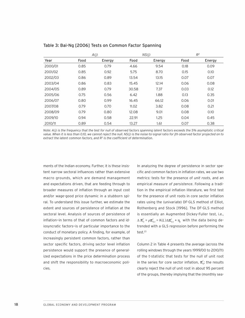
Table 3 presents the test statistics A(j) (columns 2 and
3), Noise-to-Signal ratio, NS(j) (columns 4 and 5), and
R2 (columns 6 and 7) for rolling samples from 2000/01
to 2010/11. The A(j) statistics are substantially higher
than 0.10, indicating the rejection of null of exact span-
ning, while the NS(j) and R2 statistics indicate that the
degree of spanning is weak at best with the exception
of the last two years where one sees, to some extent,
the importance of energy infl ation in driving core sec-
tor infl ation. Overall, the results indicate that food and
energy sectors do not explain the latent or common
factors underlying core sector infl ation rates and that
the explanation for the dynamics of core sector infl a-
tion will have to come from somewhere else.
To further eliminate higher-order effects of food and
energy emanating from input-output considerations
and supply shocks leading to wage-price linkages
through wage-good prices, we also estimate the com-
mon factor structure on the controlled core sector
residuals:
CO-RESit
= ΛiH
t‘ +
tz
i, i = 1, …, 54; t = 1, …., T. (6)
Ht = Φ(L)H
t-1 + ξ
t (7)
Reminiscent of core sector infl ation, we fi nd that be-
tween 2007/08 and 2009/10 a single factor is gener-
ating between 50 and 70 percent of the variation for
controlled core sector residuals (see Figure 6—dashed
blue curve in the upper panel and brown bars in the
lower panel, respectively). The period 2002/03 to
2004/05 displays a precedent similar to that for πcit,
although in the last year of the sample multiple fac-
tors are detected, with explained variation same as in
2009/10. During the period of multiple common fac-
tors (3), (2002/03 to 2004/05), a declining fraction of
the variation is being explained. In summary, the fi nd-
ing that, on average, fewer common factors explain
more of the variation in Indian core sector infl ation is
supported by the factor analysis on CO-RESit
.
The finding that fewer common factors explain a
larger proportion of variation in sector infl ation rates,
combined with the results on comovement of the pre-
vious section, indicate an emerging consensus about
trending infl ation in the sectoral price determination
process if these common factors are also found to be
increasingly persistent. We turn to this issue in the
next subsection.
Extent and Source of Infl ation Persistence
It has been surmised that the current level of high
infl ation is explained by unrelenting supply side and
international causes related to food and energy seg-
18 GLOBAL ECONOMY AND DEVELOPMENT PROGRAM
ments of the Indian economy. Further, it is these insis-
tent narrow sectoral infl uences rather than extensive
macro grounds, which are demand management
and expectations driven, that are feeding through to
broader measures of infl ation through an input cost
and/or wage-good price dynamic in a stubborn spi-
ral. To understand this issue further, we estimate the
extent and sources of persistence of infl ation at the
sectoral level. Analysis of sources of persistence of
infl ation—in terms of that of common factors and id-
iosyncratic factors—is of particular importance to the
conduct of monetary policy. A fi nding, for example, of
increasingly persistent common factors, rather than
sector specifi c factors, driving sector level infl ation
persistence would support the presence of general-
ized expectations in the price determination process
and shift the responsibility to macroeconomic poli-
cies.
In analyzing the degree of persistence in sector spe-
cifi c and common factors in infl ation rates, we use two
metrics: tests for the presence of unit roots, and an
empirical measure of persistence. Following a tradi-
tion in the empirical infl ation literature, we fi rst test
for the presence of unit roots in core sector infl ation
rates using the (univariate) DF-GLS method of Elliot,
Rothenberg and Stock [1996]. The DF-GLS method
is essentially an Augmented Dickey-Fuller test, i.e.,
Δ πcit = ρπc
it-1 = K(L)Δπc
it-1 + η
t with the data being de-
trended with a GLS regression before performing the
test.23
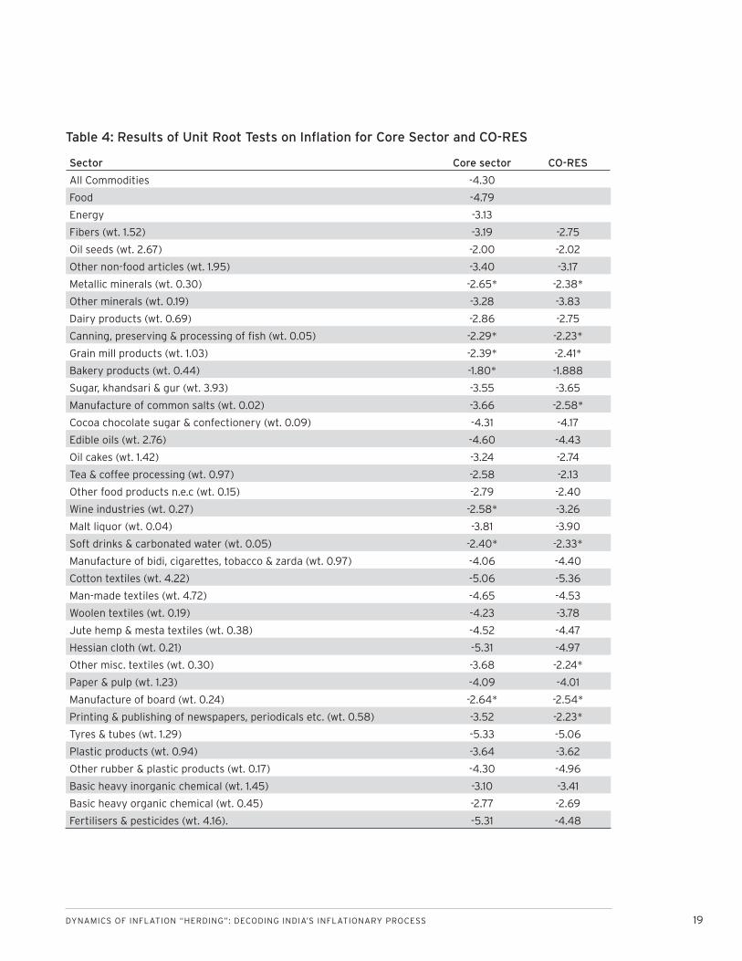
Column 2 in Table 4 presents the average (across the
rolling windows through the years 1999/00 to 2010/11)
of the t-statistic that tests for the null of unit root
in the series for core sector infl ation, πcit; the results
clearly reject the null of unit root in about 95 percent
of the groups, thereby implying that the (monthly sea-
A(j) NS(j) R2
Year Food Energy Food Energy Food Energy
2000/01 0.85 0.79 4.66 9.54 0.18 0.09
2001/02 0.85 0.92 5.75 8.70 0.15 0.10
2002/03 0.86 0.89 13.54 13.15 0.07 0.07
2003/04 0.86 0.83 15.45 12.14 0.06 0.08
2004/05 0.89 0.79 30.58 7.37 0.03 0.12
2005/06 0.75 0.56 6.42 1.88 0.13 0.35
2006/07 0.80 0.99 16.45 66.12 0.06 0.01
2007/08 0.79 0.70 11.02 3.82 0.08 0.21
2008/09 0.79 0.80 12.08 9.01 0.08 0.10
2009/10 0.94 0.58 22.91 1.25 0.04 0.45
2010/11 0.89 0.54 13.27 1.61 0.07 0.38
Table 3: Bai-Ng [2006] Tests on Common Factor Spanning
Note: A(j) is the frequency that the test for null of observed factors spanning latent factors exceeds the 5% asymptotic critical value. When it is less than 0.10, we cannot reject the null. NS(j) is the noise-to-signal ratio for jth observed factor projected on to extract the latent common factors, and R2 is the coeffi cient of determination.
DYNAMICS OF INFLATION “HERDING”: DECODING INDIA’S INFLATIONARY PROCESS 19
Sector Core sector CO-RES
All Commodities -4.30
Food -4.79
Energy -3.13
Fibers (wt. 1.52) -3.19 -2.75
Oil seeds (wt. 2.67) -2.00 -2.02
Other non-food articles (wt. 1.95) -3.40 -3.17
Metallic minerals (wt. 0.30) -2.65* -2.38*
Other minerals (wt. 0.19) -3.28 -3.83
Dairy products (wt. 0.69) -2.86 -2.75
Canning, preserving & processing of fi sh (wt. 0.05) -2.29* -2.23*
Grain mill products (wt. 1.03) -2.39* -2.41*
Bakery products (wt. 0.44) -1.80* -1.888
Sugar, khandsari & gur (wt. 3.93) -3.55 -3.65
Manufacture of common salts (wt. 0.02) -3.66 -2.58*
Cocoa chocolate sugar & confectionery (wt. 0.09) -4.31 -4.17
Edible oils (wt. 2.76) -4.60 -4.43
Oil cakes (wt. 1.42) -3.24 -2.74
Tea & coffee processing (wt. 0.97) -2.58 -2.13
Other food products n.e.c (wt. 0.15) -2.79 -2.40
Wine industries (wt. 0.27) -2.58* -3.26
Malt liquor (wt. 0.04) -3.81 -3.90
Soft drinks & carbonated water (wt. 0.05) -2.40* -2.33*
Manufacture of bidi, cigarettes, tobacco & zarda (wt. 0.97) -4.06 -4.40
Cotton textiles (wt. 4.22) -5.06 -5.36
Man-made textiles (wt. 4.72) -4.65 -4.53
Woolen textiles (wt. 0.19) -4.23 -3.78
Jute hemp & mesta textiles (wt. 0.38) -4.52 -4.47
Hessian cloth (wt. 0.21) -5.31 -4.97
Other misc. textiles (wt. 0.30) -3.68 -2.24*
Paper & pulp (wt. 1.23) -4.09 -4.01
Manufacture of board (wt. 0.24) -2.64* -2.54*
Printing & publishing of newspapers, periodicals etc. (wt. 0.58) -3.52 -2.23*
Tyres & tubes (wt. 1.29) -5.33 -5.06
Plastic products (wt. 0.94) -3.64 -3.62
Other rubber & plastic products (wt. 0.17) -4.30 -4.96
Basic heavy inorganic chemical (wt. 1.45) -3.10 -3.41
Basic heavy organic chemical (wt. 0.45) -2.77 -2.69
Fertilisers & pesticides (wt. 4.16). -5.31 -4.48
Table 4: Results of Unit Root Tests on Infl ation for Core Sector and CO-RES

20 GLOBAL ECONOMY AND DEVELOPMENT PROGRAM
Sector Core sector CO-RES
Paints varnishes & lacquers (wt. 0.50) -3.58 -4.09
Dyestuffs & indigo (wt. 0.17) -4.11 -3.99
Drugs & medicines (wt. 2.53) -4.14 -4.46
Perfumes, cosmetics, toiletries, etc. (wt. 0.98) -3.13 -3.15
Turpentine, synthetic resins, plastic materials, etc. (wt. 0.75) -4.02 -4.00
Matches, explosives & other chemicals n.e.c. (wt 0.94) -3.04 -3.66
Structural clay products (wt. 0.23). -3.63 -3.16
Glass, earthenware, chinaware & their products (wt. 0.24) -4.41 -4.35
Cement (wt. 1.73) -5.98 -3.80
Cement slate & graphite products (wt. 0.32) -4.16 -3.89
Basic metals & alloys (wt. 6.21) -6.74 -4.71
Non-ferrous metals (wt. 1.47) -2.59* -2.72*
Metal products (wt. 0.67) -4.10 -2.92
Non-electrical machinery & parts (wt. 3.38) -5.68 -3.66
Valve (wt all types) (wt. 0.09) -4.48 -4.83
Electrical machinery (wt. 4.98) -4.85 -3.66
Enameled copper wires (wt. 0.15) -5.08 -3.82
Locomotives railway wagon & parts (wt. 0.32) -5.80 -5.10
Motor vehicles, motorcycles, scooters, bicycles & parts (wt. 3.98) -3.44 -3.23
Table 4: Results of Unit Root Tests on Infl ation for Core Sector and CO-RES (cont.)
* Denotes: Not signifi cant at 5 percent critical values associated with optimal lag length.
sonally unadjusted) core sectoral infl ation process in
India is stationary.24 The results remain the same even
after controlling for food and energy price effects
(Column 3 in Table 4).
Rolling sample estimates of the sum of autoregressive
coeffi cients, ρ, indicate that there is an increase in per-
sistence in recent times across the board as refl ected
in the upward movement of cross-sectional weighted
moments of ρit for core sectors. After 2004/05, while
persistence of food infl ation and, to some extent, en-
ergy infl ation has been variable, for core sector infl a-
tion the estimates show a clear upward trend (Figure
7). Persistence of broader measures of infl ation is not
due to the behavior of food and energy price changes
alone, therefore, the explanation lies somewhere else.
Based on the fi ndings that the core sector infl ation
rates are increasingly driven by common factors and
are also progressively more persistent, we analyze
whether the latter pattern is determined by ever more
persistent common factors, or, by sector specifi c fac-
tors?
The basic factor framework for large dimensional
panels used earlier in this section allows us to for-
mally investigate this proposition using the frame-
work of PANIC (“Panel Analysis of Non-stationarity
in Idiosyncratic and Common Factors”) developed in

DYNAMICS OF INFLATION “HERDING”: DECODING INDIA’S INFLATIONARY PROCESS 21
Bai and Ng [2004]. PANIC test procedures allows one
to extract common and idiosyncratic factors from a
panel of data in the fi rst stage, and derive the diag-
nostics for testing for unit roots in extracted common
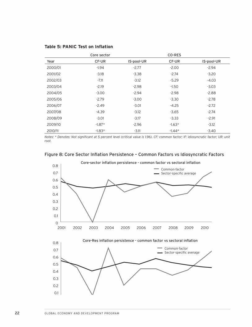
and idiosyncratic factors in the second stage. Results
presented in Table 5 indicate that one can strongly
reject the null of unit root in both common factors
and idiosyncratic factors for core sector, as well as
controlled core sector residuals, for the rolling sam-
ples up to 2008/09, reinforcing the earlier fi ndings
that India’s infl ation process is devoid of a unit root.
However, common factors for both groups display
unit root behavior for 2009/10 and 2010/11. To obtain
further insight into these dynamics, the extent of- and
the time variation in- the persistence of common and
sector specifi c factors is evaluated.
Figure 8 plots the average measures of persistence
for common and sectoral factors obtained from es-
timates of equations (4) and (6). The time evolution
of this measure25 for common factors pertaining to
core sector, πcit, shows that these have become more
enduring in recent years; on the other hand, while id-
iosyncratic factors are persistent, there is no distinct
change in the degree of their persistence (upper panel
of Figure 8). Almost identical fi ndings are obtained
for estimates of the persistence of common and idio-
syncratic factors relevant to CO-RESit
(lower panel of
Figure 8).
It is clear that in recent years (2008/09 to 2010/11),
for the most part, a small number of common fac-
tors are found to be far more durable in the infl ation
dynamic rather than sector specifi c pressures. India’s
Figure 7: Infl ation Persistence
2001 2002 2003 2004 2005 2006 2007 2008 2009 2010 2011
0.9
0.8
0.7
0.6
0.5
0.4
0.3
0.2
0.1
0
Inflation persistence - WPI-All, food, energy, and core-sector inflation
WPI-All
Food
Energy
Core-sector
22 GLOBAL ECONOMY AND DEVELOPMENT PROGRAM
2001 2002 2003 2004 2005 2006 2007 2008 2009 2010
Core-sector inflation persistence - common factor vs sectoral inflation
Common-factorSector-specific average
0.8
0.7
0.6
0.5
0.4
0.3
0.2
0.1
Core-Res inflation persistence - common factor vs sectoral inflation
0.8
0.7
0.6
0.5
0.4
0.3
0.2
0.1
0
Common-factorSector-specific average
Figure 8: Core Sector Infl ation Persistence – Common Factors vs Idiosyncratic Factors
Core sector CO-RES
Year CF-UR IS-pool-UR CF-UR IS-pool-UR
2000/01 -1.94 -2.77 -2.00 -2.94
2001/02 -3.18 -3.38 -2.74 -3.20
2002/03 -7.11 -3.12 -5.29 -4.03
2003/04 -2.19 -2.98 -1.50 -3.03
2004/05 -3.00 -2.94 -2.98 -2.88
2005/06 -2.79 -3.00 -3.30 -2.78
2006/07 -2.49 -3.01 -4.25 -2.72
2007/08 -4.39 -3.12 -3.65 -2.74
2008/09 -3.01 -3.17 -3.33 -2.91
2009/10 -1.87* -2.96 -1.63* -3.12
2010/11 -1.83* -3.11 -1.44* -3.40
Table 5: PANIC Test on Infl ation
Notes: * Denotes: Not signifi cant at 5 percent level (critical value is 1.96). CF: common factor; IF: idiosyncratic factor; UR: unit root.
DYNAMICS OF INFLATION “HERDING”: DECODING INDIA’S INFLATIONARY PROCESS 23
most recent fl irtation with high core sector infl ation
is likely to be difficult to rein in, regardless of the
identity of the common factors driving the process. If
policy makers had formally investigated the change in
the degree of persistence we would have been spared
the optimistic “rolling forecasts” alluded to in the in-
troduction.
Our results in this subsection convey that while India’s
recent infl ationary experience does not follow a unit
root process, in recent times the dynamic is character-
ized by increasing persistence. The common factors
underlying this wide ranging (across sectors) mani-
festation has been exhibiting a similar—increasingly
“headstrong”—and possibly disturbing trait (from the
standpoint of prospective policy effectiveness). These
fi ndings collectively suggest that bringing infl ation
down to “acceptable” levels at this (overdue) stage is
likely to be an onerous task for policy makers.
24 GLOBAL ECONOMY AND DEVELOPMENT PROGRAM
PURE INFLATION GAUGES (PIGS) AS A MEASURE OF POLICY (IN-) EFFECTIVENESS
An important prerequisite for the effective con-
duct of monetary policy in targeting infl ation is
to identify the aggregate source of changes in com-
modity prices. While an undue amount of effort is
placed on identifying the sources of variation in aggre-
gate or headline infl ation—in terms of macroeconomic
impulses, critical sector specifi c supply side shocks,
etc. usually through VAR and related methods—very
little work has been done in exploring the signifi-
cance of aggregate or common factors in explain-
ing the variation in disaggregated sectoral infl ation.
Understanding the sources of variation in infl ation at
a sectoral level is important for two reasons. First, sec-
toral infl ation as against aggregate infl ation is more
closely associated with the welfare effects of macro or
monetary policies. Second, it helps to understand how
much of observed variation in sector infl ation rates
is due to economy wide aggregate factors refl ecting,
inter alia, generalized infl ation expectations or sector
specifi c idiosyncratic factors. Decomposing sectoral
price variations into those associated with common
(macro) factors, as against sector specific factors,
can provide a better indication of the effectiveness of
macro and monetary policies in containing infl ation-
ary pressures than measures of headline infl ation that
are prone to well known aggregation biases.
Constructed aggregate indices such as WPI-all may
not reflect the correlation and response of goods
prices with respect to aggregate source(s) and, be-
ing an (weighted) average of disaggregated prices,
indices may be unduly infl uenced by select commod-
ity groups. Various methods, for example trimmed
means, were developed to construct a core infl ation
measure that is less sensitive to outliers in underlying
disaggregated data. While these methods provide sta-
tistically robust measures of aggregate infl ation, they
do not correspond to a notion of aggregate infl ation
that is common to all disaggregated groups (Bryan et.
al. [1997]). More specifi cally, no economic interpreta-
tion can be attached to such measures as we can do
with the common factors driving the panel of disag-
gregated infl ation.
In order to understand to what extent the observed
sectoral price changes are driven by aggregate fac-
tors, that have equiproportional or differential effect
on all or some of commodity groups, and sector spe-
cifi c factors, we specify that sectoral infl ation rates
can be decomposed into three components: (i) a
pure infl ation component that affects all commodity
groups equiproportionately; (ii) aggregated relative
inflation components that affect some commodity
groups more than others; and (iii) idiosyncratic com-
ponents that are sector specifi c, that is:
πit = at + Λ
iF
t‘ + u
i t, i = 1, …, 63; t = 1, …., T. (8)
where πit are measured sector infl ation rates (in WPI-
all); at is the pure infl ation factor, which has equipro-
portional effects on all sectoral price changes and, by
construction, is orthogonal to (aggregated) relative
price factors and idiosyncratic factors. Ft is the vec-
tor of (aggregated) relative price factors, Λ is the
matrix of common factor loadings and ui t represent
the sector specifi c components of infl ation. This de-
composition can be interpreted either as a time series
of cross-sectional distribution of infl ation rates, or a
cross section of time series of each of the sector spe-
cifi c infl ation rates.
We label at “pure” because, by construction, its
changes are uncorrelated with relative price changes
at any point in time. In a simple fl exible-price classical
model where money is neutral, pure infl ation would
equal the money growth rate. More generally, it cor-

DYNAMICS OF INFLATION “HERDING”: DECODING INDIA’S INFLATIONARY PROCESS 25
responds to the famous thought experiment that
economists have used since Hume (1752): “imagine
that all prices increase in the same proportion, but no
relative price changes”. Measurement of pure infl a-
tion from the disaggregated sectoral infl ation rates,
which may not be similar to that based on WPI-all, will
help us answer two important questions: (i) to what
extent is the observed variation in sectoral prices due
to idiosyncratic or sector specifi c factors as against
“pure” or correlated relative price shocks; and (ii) is
there an increase in the pure inflation component
in recent times indicating an increase in generalized
infl ationary expectations due to—not implausibly—lax
macroeconomic management or accommodative
monetary policies.
Methodology for Measuring PIGs
Following the cross-sectional regression approach of
Fama and MacBeth [1973] in the empirical asset pric-
ing literature, we postulate that the cross-sectional
distribution of disaggregated sector infl ation rates
can, at any given time period, be explained by the
sensitivities of each sector to aggregate or sub-ag-
gregate shocks, sector specifi c shocks and a common
shock, i.e.,
πit+h = a
t + γ
t Λ + η
i, i = 1, …, 63; t = 1, …., T. (9)
where the variables are as defi ned above.
We follow a two-stage procedure for implementing
this approach:26
1. At the fi rst stage, we estimate, Λ the factor sen-
sitivity matrix or factor loadings, by undertaking a
principal component analysis on the panel of infl a-
tion rates πit measured up to time t using the relation
πit = at + Λi
Ft
‘ + ui t.
2. At the second stage, we regress cross-sectoral infl a-
tion rates for time period t+1 on the estimated factor
sensitivities from stage 1, i.e., πit = a + γΛ + ηi. The
intercept term in this cross section regression, as ex-
plained above, is pure infl ation for period t+1.
3. This procedure is repeated for all t+h, h = 1…T, and
the time series of pure infl ation are extracted as at+h
.
The cross-sectional approach to the measurement of
pure infl ation is particularly useful since it can eas-
ily be modifi ed to include other factors infl uencing
cross-sectional differences in infl ation rates, thereby
making the estimate of pure infl ation relatively more
robust. There are concerns with the methodology.
First, the factor sensitivities that we use as control
variables in the second stage regression are unob-
servable and hence have to be estimated from the
fi rst stage time series model, which introduces an er-
rors-in-variables problem. To mitigate this problem, as
suggested by Fama and MacBeth [1973] in the context
of the CAPM27, we use sub-aggregate indices of infl a-
tion rather than the most detailed commodity level in-
fl ation rates. Also, the errors-in-variables problem has
consequences for the inference related to the slope
coeffi cients in the second stage regression and much
less effect on the point estimate of the intercept term,
i.e. the pure inflation term in the present context,
which is the focus of our exercise.
In Figure 9, we overlay on WPI headline inflation
for the April 2001 to March 2011 period, pure infl a-
tion gauges (PIGs) extracted from aggregate infla-
tion (pure-all) and core sector infl ation (pure-core).28
While, like most measures of inflation in India, the
three series are highly variable, the variability of pure-
core is the least, with headline infl ation as the most
variable and pure-all in between the other two series.
Both pure-all and pure-core are highly correlated with

26 GLOBAL ECONOMY AND DEVELOPMENT PROGRAM
overall infl ation—coeffi cients of around 0.9—but the
differences between the three series in the fi gure are
eye-catching. The most recent trough in headline in-
fl ation may have given policy makers false indication
of muted underlying infl ationary pressure. While ag-
gregate infl ation by the end of 2008/09 had declined
to about 1 percent (from about 8 percent in 2007/08),
pure-all and pure-core were running at, respectively,
3.5 percent and 2.6 percent (in contrast to the head-
line infl ation, the most recent trough for pure-core
and pure-all was 2005/06 and not 2008/09). The de-
cline in (and the level of) headline infl ation in 2008/09
may have conveyed to the authorities that they had
more elbow room for monetary easing (or less need/
more time for tightening) than was the case looking
at infl ation measures corrected for sectoral and id-
iosyncratic shocks. The steep decrease in aggregate
infl ation (with even talk of generalized defl ation) may
have informed the hasten-slowly (“lack of alacrity”)
strategy of the RBI; the resultant extended period of
softer-than-warranted policy allowed infl ationary ex-
pectations to take hold (since pure-all infl ation, while
Figure 9: PIGs
2001 2002 2003 2004 2005 2006 2007 2008 2009 2010 20110
2
4
6
8
10
12Pure Inflation Gauge
0.86536 0.86787
WPI-All
Pure Inflation - Core
Pure Inflation - All
Linear

DYNAMICS OF INFLATION “HERDING”: DECODING INDIA’S INFLATIONARY PROCESS 27
declining, was running at or near the upper end of
the erstwhile policy comfort zone). The ensuing most
recent period of high infl ation followed, with headline
infl ation staying stubbornly in the 7-11 percent range,
and even pure-core in excess of 5 percent, for most of
the last two years.
If PIGs, in conjunction with our other fi ndings, for ex-
ample, on persistence had been used as a measure of
underlying (pure) infl ationary pressures, the monetary
authorities may not have been sanguine regarding the
timeliness of initiating anti-infl ationary policies.

28 GLOBAL ECONOMY AND DEVELOPMENT PROGRAM
CONCLUSIONS
In the context of public discourse about infl ation it is
often the case that a few critical sectors are singled
out as drivers of overall infl ation. Typically, these fac-
tors are claimed by policy makers to be outside their
purview, thus absolving themselves—at least partially
–from the responsibility of infl ation control. In this pa-
per we propose a consistent empirical framework to
validate such claims. Based on the analysis of a large
panel of sector level infl ation rates we attempted to
determine how the empirical properties of the Indian
infl ationary dynamic have evolved over the last de-
cade. We sought to impart methodological rigor along
a four dimensional metric, viz., KDFs, comovement,
persistence, and untangling aggregate infl ation into
“pure” and correlated components, which can be part
of the operational tool kit for infl ation management.
Overall our fi ndings allow us to make the following
statement: the recent bout of high, persistent and
widespread (across sectors) inflation is not on ac-
count of food and energy. Firstly, we fi nd that the ex-
tant bout of elevated infl ation is coincident with right
skewness of pdfs of sectoral prices. This is unlike the
previous episode of high infl ation in the mid-1990s,
which was not characterized by large right skew-
ness. Secondly, the pattern of infl ation in the current
period suggests that it has diffused widely across
sectors, that is, there is increasing comovement mea-
sured by both intuitive “single factor” methods and
from deploying somewhat intricate generic methods
like dynamic factor analysis. Thirdly, the number of
statistically identifi ed common factors has declined
since 2004/05, and these explain a larger fraction of
the variation in infl ation. Fourthly, recent times are
characterized by increasing persistence of overall and
core sector infl ation. Fifthly, persistence of common
factors has increased in recent years; while specifi c
factors are persistent there is no distinct change in
the degree over this period. All this is likely to make it
more diffi cult for anti-infl ationary policy to gain trac-
tion this time round compared to the past. It may have
dawned somewhat late on the RBI that the underlying
drivers were getting more stubborn, hence the recent
robust hikes in policy interest rates that have been out
of character from earlier behavior. Lastly, we fi nd that
if policy makers had used a pure infl ation measure
(PIGs) they would not have underestimated the under-
lying infl ation in 2008/09, which informed their policy
stance for rather too long.
DYNAMICS OF INFLATION “HERDING”: DECODING INDIA’S INFLATIONARY PROCESS 29
REFERENCES
Bai, Jushan, and Serena Ng. 2002. “Determining
the Number of Factors in Approximate Factor
Models”. Econometrica. Vol. 70. pp. 191-221.
Bai, Jushan, and Serena Ng. 2004. “A PANIC Attack on
Unit Roots and Cointegration”. Econometrica. Vol.
72 (4). pp. 1127-1177.
Bai, Jushan, and Serena Ng. 2006. “Evaluating Latent
and Observed Factors in Macroeconomics and
Finance”. Journal of Econometrics. Vol. 131. pp.
507-537.
Bai, Jushan, and Serena Ng. 2007. “Determining the
Number of Primitive Shocks in Factor Models”.
Journal of Business and Economic Statistics. Vol.
25 (1). pp. 52-60.
Bai, Jushan, and Serena Ng. 2008. “Large Dimensional
Factor Analysis”. Foundations and Trends in
Econometrics. Vol. 3 (2). pp 89-163.
Balakrishnan, Pulapre. 1991. Pricing and Infl ation in
India, Oxford University Press, Delhi.
Ball, Laurence, and Sandeep Mazumdar. 2011. “The
Evolution of Inflation Dynamics and the Great
Recession”. Paper for the Brookings Panel on
Economic Activity. March.
Bal l , Laurence and Gregory Mankiw. 1992a.
“Asymmetric Price Adjustment and Economic
Fluctuations”. NBER Working Paper No. 4089.
June.
Ball, Laurence and Gregory Mankiw. 1992b. “Relative-
Price Changes as Aggregate Supply Shocks.
NBER Working Paper No. 4168. September.
Bernanke, Ben, and Jean Boivin. 2001. “Monetary
Policy in a Data-Rich Environment”. NBER
Working Paper No. 8379. July.
Bhattacharya, B. B., and S. Kathuria. 1995. “Dynamics
of Infl ation in India”. Paper presented at the 31st
Annual Conference of the Indian Econometric
Society.
Blejer, Mario. 1983. “On the Anatomy of Inflation:
The Variability of Relative Commodity Prices
in Argentina”. Journal of Money, Credit, and
Banking. Vol. 15 (4). pp. 469-488.
Bryan, Michael, Stephen G. Cecchetti and Rodney L.
Wiggins II. 1997. “Effi cient Infl ation Estimation”.
NBER Working Paper No. 6183.
Chowdhry, Bhagwan, Richard Roll and Yihong Xia.
2005. “Extracting Infl ation from Stock Returns
to Test Purchasing Power Parity”. American
Economic Review. Vol. 95. pp. 255-276.
Elliot, Graham, J. Rothenberg and J. H. Stock. 1996.
“Efficient Tests for Autoregressive Unit Root”.
Econometrica. Vol. 64. pp. 813-836.
Fama, Eugene, and James D. MacBeth. 1973. “Risk,
Return and Equilibrium: Empirical Tests”. Journal
of Political Economy. Vol. 81 (3). pp. 607-636.
Fischer, Stanley. 1981. “Relative Shocks, Relative Price
Variability, and Infl ation”. Brookings Papers on
Economic Activity. Vol. 2. pp. 381-431.
Government of India. 1991, 1992, 1993. Union
Government Budget Documents. Ministry of
Finance. New Delhi.
Hercowitz, Zvi. 1981. “Money and the Dispersion of
Relative Prices”. Journal of Political Economy. Vol
89 (2). 328-356.

30 GLOBAL ECONOMY AND DEVELOPMENT PROGRAM
Hume, David. 1752. Political Discourses. Reprinted in
“Essays, Moral, Political, and Literary”, edited by
Eugene F. Miller, Liberty Fund.
Hwang, Soosung, and Mark Salmon. 2004. “Market
Stress and Herding”. Journal of Empirical
Finance. Vol. 11. pp. 585-616.
IMF. 2011. World Economic Outlook. April.
Mills, Frederick C. 1927. “The Behaviour of Prices”.
NBER. pp. 251-286.
Mishra, Prachi, and Devesh Roy. 2011. “Explaining
Infl ation in India: The Role of Food Prices”. Paper
for the India Policy Forum Conference, New Delhi.
July.
Ng, Serena and Pierre Perron, 2001. “Lag Length
Selection and the Construction of Unit Root Tests
with Good Size and Power”. Econometrica Vol. 69.
pp 1519-1554.
Patra, Michael, and Partha Roy. 2010. “Inflation
Expectations and Monetary Policy in India: An
Empirical Exploration”. IMF Working Paper.
March.
Reis, Ricardo, and Mark W. Watson. 2010. “Relative
Goods’ Prices, Pure Inflation, and the Phillips
Correlation”. American Economic Journal
Macroeconomics.
Roy, Sudipta, and Gangadhar Darbha. 2000. “Dynamics
of Money, Output and Price Interaction—Some
Indian Evidence”. Economic Modelling. Vol. 17. pp.
559-588.
Sheshinski, Eytan, and Yoram Weiss. “Infl ation and
Costs of Price Adjustment”. Review of Economic
Studies. Vol. 44. pp. 287-303.
Srinivasan, T. N. 2008. “Price Indices and Infl ation
Rates”. Economic and Political Weekly. pp. 217-
223. June 28.
Stock, James, and Mark Watson. 2002. “Has the
Business Cycle Changed and Why?” NBER
Working Paper No. 9127. August.
Stock, James, and Mark Watson. 2005. “Implications
of Dynamic Factor Models for VAR Analysis”.
NBER Working Paper No. 11467. July.
Subbarao, Duvuuri. 2010. “Financial crisis—some old
questions and may be some new answers.” Tenth
C.D. Deshmukh Memorial Lecture delivered at
the Council for Social Development, Southern
Regional Centre, Hyderabad. August.
Vining, Daniel, and Thomas C. Elwertowski. 1976.
American Economic Review. Vol. 66 (4). pp. 699-
708.

DYNAMICS OF INFLATION “HERDING”: DECODING INDIA’S INFLATIONARY PROCESS 31
S. No Commodity groups classifi cation
1 Basic heavy inorganic chemical (wt. 1.45) core
2 Basic metals & alloys (wt. 6.21) core
3 Cotton textiles (wt. 4.22) core
4 Dairy products (wt. 0.69) core
5 Fibers (wt. 1.52) core
6 Locomotives railway wagon & parts (wt. 0.32) core
7 Metallic minerals (wt. 0.30) core
8 Paper & pulp (wt. 1.23) core
9 Structural clay products (wt. 0.23) core
10 Tyres & tubes (wt. 1.29) core
11 Wine industries (wt. 0.27) core
12 Basic heavy organic chemical (wt. 0.45) core
13 Canning, preserving & processing of fi sh (wt. 0.05) core
14 Glass, earthenware, chinaware & their products (wt. 0.24) core
15 Malt liquor (wt. 0.04) core
16 Man-made textiles (wt. 4.72) core
17 Manufacture of board (wt. 0.24) core
18 Motor vehicles, motorcycles, scooters, bicycles & parts (wt 3.98) core
19 Non-ferrous metals (wt. 1.47) core
20 Oil seeds (wt. 2.67) core
21 Other minerals (wt. 0.19) core
22 Plastic products (wt. 0.94) core
23 Enameled copper wires (wt. 0.15) core
24 Hessian cloth (wt. 0.21) core
25 Valve (wt all types) (wt. 0.09) core
26 Cement (wt. 1.73) core
27 Fertilizers & pesticides (wt. 4.16) core
28 Grain mill products (wt. 1.03) core
29 Metal products (wt. 0.67) core
30 Other non-food articles (wt. 1.95) core
31 Other rubber & plastic products (wt. 0.17) core
32 Printing & publishing of newspapers, periodicals etc. (wt. 0.58) core
33 Soft drinks & carbonated water (wt. 0.05) core
34 Woolen textiles (wt. 0.19) core
35 Non-electrical machinery & parts (wt. 3.38) core
36 Bakery products (wt. 0.44) core
APPENDIX: LIST OF COMMODITY GROUPS
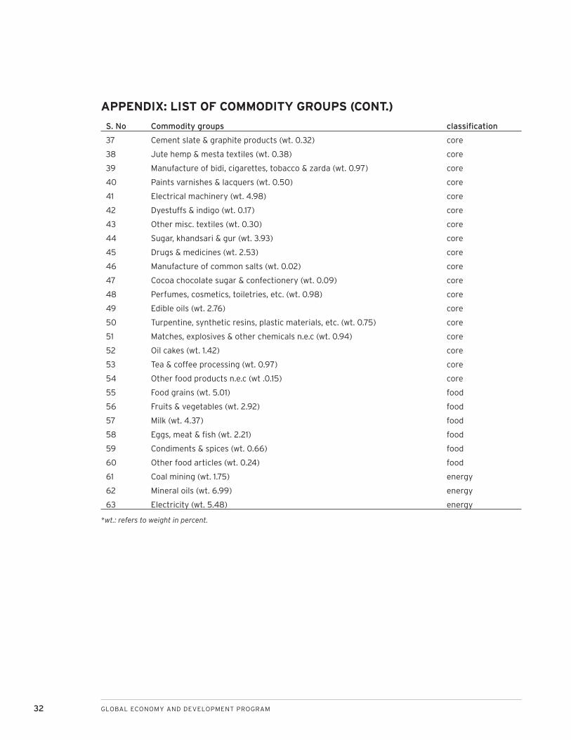
32 GLOBAL ECONOMY AND DEVELOPMENT PROGRAM
S. No Commodity groups classifi cation
37 Cement slate & graphite products (wt. 0.32) core
38 Jute hemp & mesta textiles (wt. 0.38) core
39 Manufacture of bidi, cigarettes, tobacco & zarda (wt. 0.97) core
40 Paints varnishes & lacquers (wt. 0.50) core
41 Electrical machinery (wt. 4.98) core
42 Dyestuffs & indigo (wt. 0.17) core
43 Other misc. textiles (wt. 0.30) core
44 Sugar, khandsari & gur (wt. 3.93) core
45 Drugs & medicines (wt. 2.53) core
46 Manufacture of common salts (wt. 0.02) core
47 Cocoa chocolate sugar & confectionery (wt. 0.09) core
48 Perfumes, cosmetics, toiletries, etc. (wt. 0.98) core
49 Edible oils (wt. 2.76) core
50 Turpentine, synthetic resins, plastic materials, etc. (wt. 0.75) core
51 Matches, explosives & other chemicals n.e.c (wt. 0.94) core
52 Oil cakes (wt. 1.42) core
53 Tea & coffee processing (wt. 0.97) core
54 Other food products n.e.c (wt .0.15) core
55 Food grains (wt. 5.01) food
56 Fruits & vegetables (wt. 2.92) food
57 Milk (wt. 4.37) food
58 Eggs, meat & fi sh (wt. 2.21) food
59 Condiments & spices (wt. 0.66) food
60 Other food articles (wt. 0.24) food
61 Coal mining (wt. 1.75) energy
62 Mineral oils (wt. 6.99) energy
63 Electricity (wt. 5.48) energy
*wt.: refers to weight in percent.
APPENDIX: LIST OF COMMODITY GROUPS (CONT.)

DYNAMICS OF INFLATION “HERDING”: DECODING INDIA’S INFLATIONARY PROCESS 33
ENDNOTESThe average WPI infl ation rate for the current fi s-
cal year is being projected by some respectable
analysts to be as high as 8.5 percent.
Brazil, Russia, India, and China.
For example, the Report of the Committee on Cap-
ital Account Convertibility, May 1997.
The government manages to borrow at negative
rates despite eleven policy rate hikes (aggregating
475 basis points) by the RBI since March 2010.
In September 1994 an agreement (without legis-
lated sanction) to phase out by 1997/98 the in-
strument of ad hoc Treasury Bills which hitherto
facilitated automatic monetisation of the budget
defi cit—the borrowing gap after all other fi nancing
instruments have been exhausted—was reached
between the RBI and the Central Exchequer. This,
in itself, did not preclude the RBI from participat-
ing in primary issues of central government secu-
rities or operating in the secondary markets for
central government debt, but it left these deci-
sions to the RBI’s discretion.
For developed economies, research on infl ation
dynamics is dominated by the Phillips curve rela-
tionship (see Ball and Mazumder [2011] and refer-
ences therein for recent examples).
The most glaring shortcoming is the coverage—
while 55 percent of India’s GDP is on account of
services, the WPI ignores it! Also, see Srinivasan
[2008].
Common factors (sources) can be likened to the
macro policy backdrop (determinants) for chang-
es in (all) infl ation measures over time, or, they
might be due to shocks that directly affect many
but not all sectors, like changes in energy prices.
Menu costs can also be interpreted as refl ect-
ing the costs which are required to eliminate the
uncertainty on behalf of consumers concerning
changes in relative (in contrast to aggregate)
1.
2.
3.
4.
5.
6.
7.
8.
9.
prices.
The Indian fi scal year is April-March.
The list of commodity groups is provided in the
Appendix at the end of the paper.
Month-on-month infl ation, annualized for the pur-
pose of scaling.
After trying out various lag lengths in (1), we have
used l = 6 to obtain ε itc since beyond this lag
length there is little change in our results.
Comovement is measured with respect to an ag-
gregate, for example, comovement between core
sector infl ation and aggregate (headline) infl a-
tion at t is: cmc-all = Σn
i=1w
i ((πc
i x πall) / (|πci x πall|)),
with wi iw denoting weight of commodity i (= 1,….,
n), and cmc-all ∈ [-1, 1]. The analogue for comove-
ment between aggregate infl ation and controlled
core sector residuals, CO-RES, should be obvious
enough.
The specifi cation is analogous to models of asset
pricing used to assess the cross-sectional disper-
sion of the factor sensitivity of assets within a
given market, where the market index itself is de-
ployed to “bifurcate” asset returns attributable to
herding and (fi rm/sector) fundamentals (Hwang
and Salmon [2004]).
“I think that there is a general fi scal-fi nancial-
monetary cause of infl ation which essentially
overrides all other considerations. Put another
way: I do not believe that, in the longer run, the
general price level is determined by the sum of
its parts....The relationship between the price of
steel, for example, and the price of wheat is a rela-
tive concept—that is, it is determined by the rela-
tive supplies and demands, and the absolute price
of each is not determined by that relationship, but
by the aggregate price level......” (Alan Greenspan
quoted in Vining and Elwertowski [1976]).
Alternatively, we could have estimated (2)
by deploying (separately) two auxiliary re-
10.
11.
12.
13.
14.
15.
16.
17.

34 GLOBAL ECONOMY AND DEVELOPMENT PROGRAM
gressors—food infl ation and energy infl a-
tion—in addition to aggregate infl ation, viz.,
πcit = α
i + β
1 i overall infl ation
t + β
2i food infl ation
t +
β3i
energy infl ation+ εit
The central foundation of the (dynamic) factor
model is that there are a small number of unob-
served common dynamic factors that produce the
observed comovements of economic time series.
These common dynamic factors are driven by
common structural economic shocks, which are
the relevant shocks that must be identifi ed for the
purposes of conducting policy analysis.
Akin to betas in the APT.
A dynamic factor model always has a static factor
representation.
The application of factor estimates to summarise
information in a data-rich environment has been
found to be valuable in forecasting exercises and
in the conduct of policy (Stock and Watson [2002]
and Bernanke and Boivin [2001]).
An expanding window rather than a rolling win-
dow approach is used as more data points become
available and, hence, more precision is obtained.
The null of unit root is a test on ρ = 0 as against
the alternative of ρ < 0 with the choice of lag
length based on MAIC for each series (Ng and Per-
ron [2001]).
Other studies have found year-on-year infl ation
to contain a unit root, which, in our view, is an ar-
tifact of the temporal aggregation involved.
When multiple common factors are found, the
measure of persistence is the weighted average
of persistence of each individual common factor
with weights being the proportion of variation at-
tributed to each of the common factors.
Chowdhry, Roll and Xia [2005] follow a similar
approach to estimate the risk free rate and the
implied infl ation rate from a cross section of stock
returns. Reis and Watson [2010], on the other
18.
19.
20.
21.
22.
23.
24.
25.
26.
hand, use the dynamic factor formulation to es-
timate the pure infl ation component in a single
step.
Capital Asset Pricing Model.
The methodology for calculating pure-core is
identical as that enunciated above for pure-all,
but would cover 54 sectors.
27.
28.

The views expressed in this working paper do not necessarily refl ect the offi cial position of Brookings, its board or the advisory council members.
© 2012 The Brookings Institution
ISSN: 1939-9383

1775 Massachusetts Avenue, NWWashington, DC 20036202-797-6000www.brookings.edu/global