ecological evaluation for environmental impact … · 3.2.1 what objective of ecological...

7

Ecological evaluation for environmental

impact assessment

Davide Geneletti

8

Contents Figures 12 Tables 14 Preface 16 1 Scope and outline of the book 18

1.1 Introduction 18 1.2 Objectives of the study 20 1.3 Outline of the book 20

Part 1 24 2 Environmental Impact Assessment and ecological evaluation 26

2.1 Introduction 26 2.2 Environmental Impact Assessment 26

2.2.1 Definition and objectives 26 2.2.2 EIA stages 28 2.2.3 The effectiveness of EIA 32 2.2.4 The future of EIA: SEA and sustainability 33

2.2.4.1 EIA and SEA 33 2.2.4.2 EIA and Sustainability 36

2.3 Ecological Evaluation 37 2.3.1 Definition and scope 37 2.3.2 Approaches 37

2.3.2.1 Objectives of the evaluation 38 2.3.2.2 Criteria 38 2.3.2.3 Criterion assessment 41

2.3.3 Shortcomings in the practice of ecological evaluation 43 2.4 Ecological evaluation and EIA 44

2.4.1 The role of ecological evaluation within EIA 44 2.4.2 Improving the application of ecological evaluation to EIA 45

2.5 Conclusions 46 3 Framing the topic and reviewing the literature 48

3.1 Introduction 48 3.2 Framing the research topic 48

3.2.1 What objective of ecological evaluation? 48 3.2.2 What stages of EIA? 49 3.2.3 What type of projects? 50 3.2.4 What type of impacts? 50

9

3.3 Reviewing the literature 52 3.3.1 Baseline study 52

3.3.1.1 Boundary of the study area 52 3.3.1.2 Designated sites vs. overall biodiversity value 53 3.3.1.3 Levels of biodiversity 54

3.3.2 Impact prediction 55 3.3.2.1 Direct habitat loss 55 3.3.2.2 Habitat fragmentation 56

3.3.3 Impact assessment 57 3.3.3.1 Valuing habitat 58 3.3.3.2 Assessing direct habitat loss 58 3.3.3.3 Assessing habitat fragmentation 59

3.3.4 One additional remark 60 3.4 Conclusions 61

4 Methodological approach for BIA of roads 64

4.1 Introduction 64 4.1.1 Geographic Information Systems 65 4.1.2 Multicriteria evaluation 65

4.2 Baseline study 67 4.2.1 Boundary of the study area 67 4.2.2 Levels of biodiversity 68 4.2.3 Target ecosystems 68

4.3 Impact prediction 70 4.3.1 Prediction of ecosystem loss 70 4.3.2 Prediction of ecosystem fragmentation 72

4.3.2.1 Fragmentation effects 72 4.3.2.2 Selecting fragmentation indicators 73 4.3.2.3 Computing fragmentation indicators 75

4.3.3 Summary 78 4.4 Impact Assessment 79

4.4.1 Valuing ecosystems 79 4.4.2 Assessing ecosystem loss 83 4.4.3 Assessing ecosystem fragmentation 84

4.4.3.1 Assessing viability 84 4.4.3.2 The EValue procedure 87 4.4.3.3 Computing fragmentation impact scores 88

4.4.4 Summary 90 4.5 Concluding remarks 91

Part 2 94 5 Case study: the Trento-Rocchetta road project 96

5.1 Introduction 96 5.2 The Trento-Rocchetta road project 96

5.2.1 Problem and proposed solution 96

10

5.2.2 Project alternatives 98 5.2.3 Role of EIA 100

5.3 Characteristics of the area 101 5.3.1 Landscape and land use 101 5.3.2 Geomorphologic setting 102 5.3.3 Ecological relevance 103 5.3.4 The administrative context 105

5.4 Conclusions 107 6 Baseline study 108

6.1 Introduction 108 6.2 Boundary of the study area 108 6.3 Land-cover mapping 111

6.3.1 Requirements 111 6.3.2 Available data 112 6.3.3 Proposed strategy 113 6.3.4 Land-cover mapping of the reference area 113

6.3.4.1 Classifying the forests 113 6.3.4.2 Classifying the TM image 114

6.3.5 Land-cover mapping of the study area 118 6.3.5.1 Object-oriented classification of remotely sensed data 118 6.3.5.2 The adopted methodology 118 6.3.5.3 Classification Results 120

6.4 The natural ecosystems 121 6.5 Concluding remarks 123

7 Impact prediction and assessment 126

7.1 Introduction 126 7.2 Impact prediction 127

7.2.1 Space occupation buffers and direct ecosystem loss 127 7.2.2 Ecosystem fragmentation 130

7.3 Impact assessment 131 7.3.1 Computing the rarity indicator 131 7.3.2 Assessing rarity values 133 7.3.3 Assessing direct ecosystem loss 136 7.3.4 Assessing viability values 137

7.3.4.1 Assessment of value functions and weights 138 7.3.4.2 Assessment of ecosystem viability values 143

7.3.5 Assessing ecosystem fragmentation 144 7.4 Performance of the six alternatives 147 7.5 Concluding remarks 150

8 Multicriteria evaluation and uncertainty analysis 154

8.1 Introduction 154 8.2 Application of MCE to the case study 157

8.2.1 Value functions, weight assignment and aggregation 157

11

8.2.2 Basic sensitivity analysis 159 8.3 Uncertainty in the baseline study 162

8.3.1 Fuzzy-boundary mapping 164 8.3.1.1 Fuzzy-boundary ecosystem map 165

8.3.2 Effects on impact scores and alternative ranking 167 8.3.3 Discussion 170

8.4 Uncertainty in the impact prediction 170 8.4.1 Considering space-occupation ranges 171 8.4.2 Discussion 173

8.5 Uncertainty in the impact assessment 174 8.5.1 Uncertainty in the assessment of rarity values 175 8.5.2 Uncertainty in the assessment of viability values 176 8.5.3 Discussion 178

8.6 Concluding remarks 179 9 Summary and conclusions 182

9.1 Introduction 182 9.2 Ecological evaluation for EIA 183 9.3 BIA of roads and its shortcomings 184 9.4 A methodological approach for BIA of roads 185

9.4.1 Contributions to the literature shortcomings 185 9.4.2 Advantages and limitations 186 9.4.3 Extension toward other types of project 187

9.5 Case study and operationalisation of the approach 188 9.5.1 Results of the case study 188 9.5.2 Data availability and tasks of the Public Administration 189

9.6 Directions for further research 191 9.6.1 Prediction of space-occupation impacts 191 9.6.2 Generation of project alternatives 192

Appendix List of the Italian EISs consulted 194 References 196 Dutch summary 208 Colour plates 210

12

Figures Figure 1.1 Outline of the book 22 Figure 2.1 Structure of this chapter 26 Figure 2.2 The role of EIA in the decision process 27 Figure 2.3 Flow-chart of the EIA stages 29 Figure 2.4 Excerpt of an impact matrix for an irrigation scheme 31 Figure 2.5 SEA and EIA in the planning process 34 Figure 2.6 The role of EIA and SEA in the mobility problem example 35 Figure 2.7 The two paths for the assignment of value scores. 41 Figure 3.1 The EIA stages considered in this research 49 Figure 3.2 Synthesis of the results of the literature review 62 Figure 4.1 Structure of the chapter 64 Figure 4.2 Operational flow of MCE 67 Figure 4.3 Diagram of the procedure to predict the ecosystem-loss impact 72 Figure 4.4 Illustration of the effects caused by a road on ecosystem patches 73 Figure 4.5 Example of core area and outer belt of a patch 75 Figure 4.6 Example of the computation of the Thiessen polygons for four ecosystem

patches 76 Figure 4.7 Example of the computation of the fragmentation indicators in the pre- and post-

project conditions 77 Figure 4.8 Schematic diagram of the impact prediction 78 Figure 4.9 Examples of computation of the rarity indicator for two ecosystem types 81 Figure 4.10 Example of functional curve for rarity 82 Figure 4.11 Procedural steps for the ecosystem evaluation 83 Figure 4.12 Procedural steps for assessing the fragmentation impact 84 Figure 4.13 Example of single-attribute and multi-attribute value function 85 Figure 4.14 Example of the assessment of the viability of an ecosystem patch 87 Figure 4.15 Example of computation of the fragmentation impact map 89 Figure 4.16 Schematic diagram of the impact assessment 90 Figure 5.1 Location of the Autonomous Province of Trento in Italy 97 Figure 5.2 The project area and its location within the APT 97 Figure 5.3 The existing road network and the two locations to be connected by the new

infrastructure 98 Figure 5.4 The six road layouts 99 Figure 5.5 Tiered EIA-SEA system for the solution of the mobility problem 100 Figure 5.6 Transversal and longitudinal view across the Adige Valley 102 Figure 5.7 The three biotopes 104 Figure 6.1 Rock cliffs along the western side of the Adige Valley 109 Figure 6.2 Example of boundary between the valley floor and the surrounding mountainous

landscape 110 Figure 6.3 The reference area and the boundary of the study area 111 Figure 6.4 Procedure followed for the classification of forests 114 Figure 6.5 Land-cover map of the reference area 117 Figure 6.6 Flow-chart of the object-oriented classification procedure 119

13

Figure 6.7 A sub-window of the ortho-photo mosaic and the result of its segmentation 119 Figure 6.8 Land-cover map of the study area 121 Figure 6.9 Map of the natural ecosystems occurring within the study area 123 Figure 7.1 The space-occupation buffer of the six alternatives displayed on top of the

ecosystem map 128 Figure 7.2 Comparison between the pre-project ecosystem map (Alt.0) and the six scenario

maps for a subset of the study area 129 Figure 7.3 Chart of the predicted ecosystem loss 130 Figure 7.4 The potential-vegetation map 132 Figure 7.5 The assessed functional curve for rarity 135 Figure 7.6 Endpoints of the score range and assessed value intervals for the isolation

indicator 139 Figure 7.7 Value regions. L=lower limit, H=higher limit 139 Figure 7.8 Profile sets and their assessed ranking 141 Figure 7.9 The assessed value functions for core area, isolation and disturbance 142 Figure 7.10 Ecosystem-viability map of Alternative 0 143 Figure 7.11 Ecosystem-viability map of Alternative 6 144 Figure 7.12 Fragmentation-impact maps of the six alternatives 146 Figure 8.1 Flow-chart of the impact analysis 156 Figure 8.2 Ecosystem-loss and ecosystem-fragmentation impact scores of the six project

alternatives 157 Figure 8.3 Diagram representing the impact table after the value assessment 158 Figure 8.4 Overall scores obtained using equal weights 159 Figure 8.5 Diagram of the overall scores versus the weight assigned to the ecosystem-loss

impact 160 Figure 8.6 The layout of Alternative 1 as a black line superimposed on a sub-window of

the ecosystem map 163 Figure 8.7 Example of crispy (a) and fuzzy (b) membership functions for soil depth-related

suitability 164 Figure 8.8 The membership function adopted in this study (a) and its effects on a generic

patch (b) 165 Figure 8.9 A sub-window of the fuzzy-boundary ecosystem map (a) compared with the

crisp boundary map (b) used for the impact analysis 167 Figure 8.10 An example of transition zone between two adjacent ecosystem patches 167 Figure 8.11 Flow chart of the procedure. The gray boxes indicate the steps repeated in the

fuzzy-boundary sensitivity analysis. 168 Figure 8.12 Comparison between the overall scores obtained using the fuzzy-boundary

and the crisp-boundary ecosystem maps 169 Figure 8.13 Flow-chart of the procedure. The gray boxes indicate the steps repeated in the

fuzzy space-occupation sensitivity analysis 172 Figure 8.14 Flow-chart of the procedure. The gray boxes indicate the steps repeated in the

sensitivity analysis related to the uncertainty in the rarity values 175 Figure 8.15 Flow chart of the procedure. The gray boxes indicate the steps repeated in the

sensitivity analysis related to uncertainty in the viability values 177 Figure 8.16 Comparison between the overall scores obtained using sharp and average

viability values 178

14

Tables Table 2.1 Overview of the criteria more often used for ecological evaluation 39 Table 2.2 Value scores for habitat connectivity 42 Table 2.3 Value scores for habitat diversity 42 Table 2.4 Value scores for habitat diversity 43 Table 2.5 Value score for landscape unit rarity 43 Table 3.1 The component of biological diversity 54 Table 3.2 An assessment example 59 Table 4.1 Space-occupation buffer of different road types in Italy 71 Table 4.2 Space-occupation buffer of roads. The width values were originally expressed

in ha/km 71 Table 4.3 Space-occupation buffer of roads in the USA 72 Table 6.1 The forest types identified in the reference area 114 Table 6.2 Confusion matrix for the classification of the TM image 116 Table 6.3 Legend of the land-cover map 117 Table 6.4 Confusion matrix of the land-cover map of the study area 120 Table 7.1 Predicted ecosystem loss caused by the six alternatives 128 Table 7.2 Ecosystem loss caused by the six alternatives expressed as a percentage of the

total actual cover of the different ecosystem type within the study area 130 Table 7.3 Computation of the rarity indicator for the relevant ecosystem types 133 Table 7.4 Sharp, minimum and maximum assessed value for the seven PAR percentages

used as a reference 135 Table 7.5 Value assessment for the relevant ecosystem types 135 Table 7.6 Predicted area losses of the different ecosystem types caused by the six

alternatives 137 Table 7.7 Ecosystem-loss impact scores (ELi) of the six alternatives 137 Table 7.8 Weight set 140 Table 7.9 Fragmentation-impact scores of the six alternatives 145 Table 7.10 Synthesis of the impact assessment results 147 Table 7.11 Performance of Alternative 1 147 Table 7.12 Performance of Alternative 2 148 Table 7.13 Performance of Alternative 3 148 Table 7.14 Performance of Alternative 4 148 Table 7.15 Performance of Alternative 5 149 Table 7.16 The performance of Alternative 6 149 Table 8.1 Raw impact scores (left-hand columns) and valued impact scores (right-hand

columns) of the six alternatives 158 Table 8.2 Frequency table obtained using an uncertainty range of 10% 161 Table 8.3 Impact scores computed with fuzzy and crisp ecosystem boundaries 169 Table 8.4 Impact scores computed by shifting the buffer width of ± 10 m 172 Table 8.5 Frequency table obtained using the 110-130 m buffer range 173 Table 8.6 Impact scores computed by shifting the buffer width of ± 20 m 173 Table 8.7 Frequency table obtained using the 100-140 m buffer range 173

15

Table 8.8 Ecosystem-loss impact scores computed using sharp, minimum, and maximum rarity values 176

Table 8.9 Ecosystem-fragmentation impact scores computed using sharp, minimum, and maximum rarity values 176

Table 8.10 Frequency table 176 Table 8.11 Impact scores obtained using average viability values 178

16

Preface This book reflects the research conducted during my stay at the International Institute for Geo-Information Science and Earth Observation (ITC) from summer 1998 through spring 2002. In this period I worked as a Young Researcher in the framework of the GETS project (TMR Programme of the European Union, contract no. ERBFMRXCT970162). My Ph.D. activity has been supervised by Prof. H.J. Scholten (Faculty of Economics, Business Administration and Econometrics, Vrije Universiteit Amsterdam), Prof. A.G. Fabbri (Geological Survey Division, ITC), and Dr. E. Beinat (Institute for Environmental Studies, Vrije Universiteit Amsterdam). I would like to express my gratitude to the three of them for their constant encouragement and suggestions throughout the different stages of the research, and for their comments on earlier versions of this book. In particular, I would like to thank Prof. Fabbri for carefully reviewing my written English. Working at ITC within the GETS network, and with the support of the Vrije Universiteit, provided me with a lively research environment. In particular, it gave me the possibility of browsing through the activity of several research groups, and of getting in touch with a number of people that supported this work in various ways. Among these people, I am especially grateful to Prof. A. Sharifi (Social Science Division, ITC), who was always willing to comment on my ideas and drafts; Prof. E. Feoli (Faculty of Biology, University of Trieste), who shared with me his view on the meaning and the applicability of ecological indicators; Dr. C.F. Chung (Spatial Data Analysis Lab., Geological Survey of Canada), who helped me in throwing the basis for Chapter 8, during a one-month stay at the Geological Survey of Canada. I would also like to acknowledge Prof. A. Cavallin (DISAT, University of Milano-Bicocca) for offering me the possibility of taking part in the GETS network, and for the support provided during the final months of the research. I shared most of the fieldwork, data collection, and “networking” trips with Dinand Alkema. He contributed to making them even nicer experiences. I should also acknowledge him for taking-up the driving during the field surveys, while I was enjoying the relaxing winescape of our study area. Living in Enschede for over three years was certainly enriched by the friendship of many people I had the luck to meet there, and to whom I am deeply grateful. This book is dedicated to the persons that received less attention than deserved during its writing, and in particular to my mother, Duccio, and Josefine.

18

1 Scope and outline of the book 1.1 Introduction

Environmental degradation and the depletion of natural resources induced by human activities have attracted steadily growing concerns in the last decades. Such concerns made evident the necessity for the planning authorities to count on sound information about the possible environmental consequences of development actions. One of the tools available to satisfy this need is represented by the procedure of Environmental Impact Assessment (EIA). This procedure involves the systematic identification and evaluation of the impacts on the environment caused by a proposed project. EIA is now applied worldwide. Its potential role in attaining sustainable development objectives was explicitly recognised during the 1992 Earth Summit held in Rio de Janeiro (United Nations 1992). The procedure of EIA generates a report, the Environmental Impact Statement (EIS), that summarises the findings of the evaluation and discusses the acceptability of the predicted environmental impacts. Such a report is submitted to the authorities to support the decision-making related to the approval of the development under consideration. The EIS is made up of a number of disciplinary studies, each one addressing specifically one category of effects (noise, radiation, etc.), or one environmental component (air, water, etc.). Among these components is ecology, as required, with varying wording, by all EIA legislations. Assessing the ecological impacts of a project means studying the way in which the project affects the viability and the value of habitats, ecosystems, and species. Leafing through EISs, one gets the impression that there is not a common framework to support the impact assessment on the ecological component. Only few analyses can be considered as standard and can be found in most of the studies. In general, there is not a common type of data, a common way of processing and organising the information, of selecting the evaluation criteria, of expressing the impacts, and so on. Conversely, other disciplinary studies that take part in the EIS (e.g., noise or air pollution assessment) appear much more structured. They tend to follow well-established procedures that guide the entire assessment, from the data collection to the discussion of the relevance of the impacts. As a consequence, ecology is often marginalised within EISs (Thompson et al. 1997). Two factors appear concomitantly responsible for such a situation. The first one is of a legislative nature. Law regulations about the treatment of ecological impacts in the EIS are often vague and make only few requirements mandatory in terms of data collection and impact assessment (Atkinson et al. 2000, Treweek 1996). The analysis of other environmental components or effects is facilitated by the existence of detailed regulations and guidelines to comply with during the impact assessment (e.g., thresholds of maximum emission allowed, water quality standards, etc.).

19

The second factor can be identified in the open issues and in the shortcomings that affect the scientific research in the field of ecological evaluation. Ecological evaluation aims at developing and applying methodologies to assess the relevance of an area for nature conservation. As such, it is to support the assessment of the impact of a proposed development by providing guidance on how to describe the ecological features within the area affected, how to value them, and how to predict the value losses caused by the development. However, limited efforts have been made in the last decade to improve the frameworks for ecological evaluation proposed during the 1970s and the 1980s, and to adapt them specifically to the evolving procedure of EIA. As a result, the assessment of the ecological component within EISs tends to be flawed, and to provide conclusions poorly supported by evidences and by clear rationales (Byron et al. 2000). The weakness of the analysis of ecological impacts, such as the loss and the fragmentation of natural ecosystems, limits the influence of these issues on the decision-making process. Ecological consequences are bound to play a minor role in the authorisation of a development because their relevance is not sufficiently stressed and justified in the EIS. This is particularly evident for developments affecting urban or man-dominated landscapes, i.e., areas usually devoid of features with a striking ecological significance. The lack of a framework to support a sound ecological evaluation causes such areas to be simply overlooked, opening the way to uncontrolled impacting activities. The challenge for ecological research is to improve the guidance provided to impact analyses so as to encourage good practice within EISs, and to eventually strengthen the consideration of ecological issues in the decision-making concerning new projects. To this end, the application of ecological evaluation to EIA has been chosen as the subject of this research. The evaluation of the ecological significance of an area can be undertaken from different perspectives, and consequently with different objectives. One of such perspectives focuses on the conservation of the biological diversity, or biodiversity. This has recently emerged as a key environmental issue to be accounted for in land-use planning: “Biodiversity is now a major driving force behind efforts to reform land management and development practices worldwide and to establish a more harmonious relationship between people and nature” (Noss and Cooperrider 1994). Among the human activities that pose the highest threat to the conservation of biodiversity is the construction of linear infrastructures, and roads in particular. Such projects represent artificial elements that cut through the landscape and interfere with the natural habitat conditions. This in turn influences the abundance and distribution of plant and animal species, i.e., the biodiversity of the areas impacted. Road networks are commonly found within most landscapes and their effects are spread to the point that the area ecologically disturbed by the presence of roads is considered to extend for as much as 15-20% of some country’s land surface (Forman 2000, Rijnen et al. 1995). In the light of these considerations, this study targets at the assessment of the impacts on biodiversity caused by road projects.

20

1.2 Objectives of the study

The overall objective of this study is to improve the application of ecological evaluation within EIAs. In particular, the study focuses on one specific target of ecological evaluations, i.e., biodiversity conservation, and on one specific type of projects, i.e., road developments. To satisfy this overall objective a number of steps are proposed. Each step has its own objective. The steps and their objectives are:

1. The description of the role played by ecological evaluation within the procedure of EIA. The objective of this step is to highlight the key-issues that need to be addressed by research in the field of ecological evaluation applied to EIA, framing the context from which this study takes the move (Chapter 2);

2. The identification of the specific research topic, that is Biodiversity Impact Assessment (BIA) of road projects, and the review of the relevant literature. The objective of this step is, on the one hand, to provide the rationale for the research topic and, on the other hand, to highlight the main limitations that affect its current applications (Chapter 3);

3. The development of a methodological approach for BIA of road projects, and in particular for three procedural stages: the baseline study, the impact prediction, and the impact assessment. The objective of this step is to provide solutions to the limitations that emerged during the literature review (Chapter 4);

4. The application of the proposed approach to a case study. The case study is represented by an infrastructure development within an alpine valley located in northern Italy: the Trento-Rocchetta road project. The objective of this step is to test the applicability of the proposed approach and to discuss issues related to its operationalisation (Chapters 5-8).

The approach proposed in this research does not aim at providing comprehensive guidance to perform BIA of road projects. Its purpose is rather to establish and discuss a basic framework that can help in making a sound BIA as routinely undertaken within EIA as other forms of impact assessment, such as noise or air pollution. For this reason, the research develops and discusses a complete case study, from the data collection and processing, to the impact assessment and the final recommendations. Being EIA a procedure regulated by law and managed by the competent Public Administration, it is crucial for research in EIA to get first-hand impressions of the problems affecting such contexts, so as to produce results that can find actual application. 1.3 Outline of the book

The outline of the book is shown in Figure 1.1. Besides the conclusions, the remainder of the book is divided into two main parts. Part 1 deals with the theoretical concepts, whereas Part 2 deals with the applications to a case study. Part 1 consists of three chapters. Chapter 2 sets the basis of the research by introducing the two key-concepts of EIA and ecological evaluation. EIA is described in its different stages, dwelling on its effectiveness in the light of the current trends in environmental management. Ecological

21

evaluation is then defined by specifying its purposes, the approaches proposed for attaining them, and the main shortcomings encountered in current practice. This allows to place ecological evaluation in the context of EIA and to draw some general guidelines to address research in this field. Chapter 3 gradually zooms into the field of ecological evaluation applied to EIA and frames the specific topic that is tackled by this book: BIA of road developments. Subsequently, a literature review is performed that scans through both the scientific publications and the practical applications, i.e., the Environmental Impact Statements. The results of the review are commented and compared with the general guidelines that emerged in Chapter 2. This allows formulating a number of critical issues that call for improvement. Starting from the analysis of such issues, Chapter 4 proposes a methodological approach for performing BIA of road developments. In particular, the approach focuses on three EIA stages (baseline study, impact prediction, and assessment) and two types of impact (habitat loss and habitat fragmentation). Part 2 is made up of four chapters. Chapter 5 provides an introduction to the case study selected to test the applicability of the approach. This is the Trento-Rocchetta project, a new road development within the Autonomous Province of Trento (Italy) for which a number of alternative layouts has been proposed. The chapter describes the characteristics of the different alternatives, as well as the main features of the area to be affected by the project. The case study is developed in the three following chapters that reflect the logical sequence of the operational steps within an EIA: baseline study, impact prediction and assessment, alternative evaluation and final recommendations. Owing to that sequence, each chapter takes the move from the findings of the previous one. However, the chapters apply clearly separated methodologies, and therefore they can also be read independently. Chapter 6 deals with the baseline study, and in particular with the problems related to delimiting the study area and mapping the land cover, so as to provide a suitable data-set for the remainder of the experimental work. Chapter 7 sees the application of the methodological approach for the prediction and the assessment of the impacts on biodiversity caused by the road alternatives. Finally, Chapter 8 complements the impact assessment by applying multicriteria evaluation for a suitability ranking of the alternatives and by testing the sensitivity of such a ranking with respect to a set of uncertainty factors related to the data and the methodologies that have been employed. The book closes with Chapter 9, which summarises the work done and offers some concluding remarks, as well as thoughts for future developments of this research.

22

Figure 1.1 Outline of the book

Part 1: Concepts

Chapter 1 Scope and outline of the book

Chapter 2 EIA and ecological evaluation

Chapter 3 Framing the topic and reviewing

the literature

Chapter 4 Methodological approach for BIA

of roads

Chapter 5 Case study: the Trento-Rocchetta

road project

Chapter 6 Baseline study

Chapter 7 Impact prediction and

assessment

Chapter 8 Multicriteria evaluation and

uncertainty analysis

Chapter 9 Summary and conclusions

Part 2: Applications

24

Part 1

26

2 Environmental Impact Assessment and ecological evaluation

2.1 Introduction

This chapter aims at introducing the topic of the research, by focusing on the two key-concepts of Environmental Impact Assessment and ecological evaluation. The chapter is structured as follows (see Figure 2.1). Section 2.2 deals with the procedure of EIA. It describes its purposes, its main stages, its effectiveness and it also pictures its evolution in the near future. Section 2.3 tackles the concept of ecological evaluation by providing an overview of its objectives and by reviewing the approaches proposed in the literature, as well as their main shortcomings. In Section 2.4, the two concepts are merged together and the role played by ecological evaluation within EIA is described. The section also summarises the main issues related to an effective application of ecological evaluation to EIA, framing the context from which the approach proposed in this research will take the move.

Figure 2.1 Structure of this chapter

2.2 Environmental Impact Assessment

2.2.1 Definition and objectives Constructing a new infrastructure; expanding a residential area; building an industrial plant; increasing the capacity of an airport. These are some typical examples of developments that, in most countries, can be carried out only if the competent planning authorities grant the authorisation. The authorisation is issued if the overall positive

Environmental Impact Assessment

(§ 2.2)

Ecological evaluation for EIA

(§ 2.4)

Ecological evaluation

(§ 2.3)

27

effects of the development are perceived to exceed the negative ones. In the past, such effects were mainly appraised on a socio-economic basis and included concerns such as the cost of the project, the related market advantages, the consequences for the quality of life, the increase in job opportunities, etc. As from the sixties, there has been a growing concern about the effects of the human activity on the environment and its consequences for the long-term viability of the planet. Issues such as the contamination of soil, water and air and the limitedness of the natural resources started to emerge and to be largely debated. Concomitantly, it became clear that developments needed to be evaluated from a wider perspective: they are to be approved if they make economic sense and if their social, as well as environmental implications are acceptable. Environmental Impact Assessment (EIA) aims at evaluating the full range of effects on the environment of a proposed project. It represents one of the tools that are employed during the authorisation process to provide decision-makers with useful information for taking a decision (see Figure 2.2). The overall goal of EIA is to encourage the consideration of environmental issues in decision-making so to “ultimately arrive at actions which are more environmentally compatible” (Canter 1995). A comprehensive definition of EIA is provided by Wathern (1988): “EIA can be described as a process for identifying the likely consequences for the biogeophysical environment and for man’s health and welfare of implementing particular activities and for conveying this information, at a stage when it can materially affect their decision, to those responsible for sanctioning the proposal.” This definition underlines the fact that EIA consists of both analytical and procedural aspects: EIA is not only to study the expected environmental impacts of a given development (analytical part), but also to ensure that the results of such a study can actually influence the decision-making process concerning the approval of the development (procedural part).

Figure 2.2 The role of EIA in the decision process (after Beinat et al. 1999)

The analytical aspects involve the methods and the techniques that are required to collect the relevant data, to identify the environmental impacts, to assess the significance

Proposal of a development

Environmental Impact Assessment

Economic Assessment

Social Assessment

Decision about the development

Are the environmental impacts acceptable?

Does it make economic sense?

Are the consequences socially acceptable?

28

of such impacts, to propose impact mitigation measures, etc. Such methods and techniques have been proposed by academics, experts and practitioners and are described in the scientific literature, and usually collected in guidelines, handbooks and the like (see for instance Canter 1995, Codorni and Malcevschi 1994). The procedural aspects define the position of EIA within the overall decision process concerning the authorisation of a project. They specify, for instance, the role assigned to the project developer and the public authorities, the time constraints to be respected, etc. The procedure of EIA is regulated by legislation, and consequently it is generally different between different countries, or even between regions of the same country. EIA first appeared in a national legislation in the USA in 1969 (National Environmental Policy Act). Ever since, it has found its way in the legislation of many countries, within both the industrial and the developing regions of the world. In the European Union context, EIA has been introduced by the Directive 85/337 (CEC 1985) and it is currently regulated by the amending Directive 97/11 (CEC 1997). These directives represent a common framework for the generation and application of national laws by each Member State. Despite the different legal prescription around the world, EIA consists of a rather standard set of logically organised stages that lead to the generation of a formal document: the Environmental Impact Statement (EIS). The next sub-section illustrates in detail the EIA stages and the role played by the different actors.

2.2.2 EIA stages The basic structure of an EIA follows the sequence of stages shown in Figure 2.3. Once decided that EIA is required for a proposed project, the process provides for the scoping of the study, the baseline description of the environmental conditions, the prediction and assessment of impacts, and finally the identification of mitigation measures and of a monitoring plan. Screening. It represents the first formal activity in an EIA and it is generally performed by the competent planning authorities. The purpose of screening is to determine whether EIA is actually required for a given project or not, i.e., whether the project is likely to have significant effects on the environment. Two broad approaches to help in determining which projects require EIA may be distinguished (Wood 2000):

1. The compilation of lists of projects and of accompanying thresholds and criteria. Such criteria can be based on technical parameters (e.g., space occupation, energy consumption, production of waste), as well as on the location of the project (e.g., within a protected area or not);

2. The establishment of a procedure for performing case-by-case examinations. Such examinations represent a sort of preliminary EIA.

The first approach is generally faster and simpler, but it is hard to provide a sound justification to the thresholds (e.g., what is the minimum length of a road project that requires an EIA?). Moreover, developers will tend to propose projects that are just below the thresholds, or to segment a big project into a set of smaller ones, in order to avoid EIA. The second approach, on the other hand, has the disadvantage of being more resource consuming and of being based on discretionary evaluations, which generate decisions that are hardly replicable. A more detailed analysis of the shortcomings and

29

advantages of both approaches can be found in Geneletti et al. (in press). However, in practice, most EIA systems adopt a hybrid approach that involves the use of lists and thresholds, as well as some discretion (Wood 2000). An example of such approach is represented by the guidance on screening issued by the European Commission (1995 a).

Figure 2.3 Flow-chart of the EIA stages

Scoping. It aims at identifying the priority issues that need to be addressed during the EIA. The relationships between human activities and all the environmental components may be so complex as to require a potentially endless study. However, EIAs are subjected to resource and time constraints. Therefore, it is crucial to mainstream the EIA toward the relevant issues, i.e., the impacts that appear to be particularly significant. Scoping is typically carried out by resorting to specific guidelines and questionnaires (see, for instance, European Commission 1995 b). It often involves some form of consultation

Screening

EIA required?

Scoping

Baseline study

Impact prediction

Impact assessment

Mitigation

Environmental Impact Statement

Review

Decision making

Monitoring

STOP

no

yes

Project rejected

Project approved

Iteration

30

with decision-makers, the scientific community, and the local population. A review of techniques for performing scoping can be found in Wood (2000). Baseline study. The baseline study consists in the description of the environmental setting of the area to be affected by the proposed development. According to the regulations provided by the Council of Environmental Quality of the USA (CEQ 1978), such a description shall “not be longer than is necessary to understand the effects of the development.” Carrying out the baseline study involves the collection and the processing of all the relevant thematic data (cartographic layers, record of environmental parameters, etc.). Most of the data are usually already existing and obtainable from the governmental agencies or the scientific literature. This information is typically complemented by field surveys, interpretation of remotely sensed data, etc. The description of the actual (i.e., pre-project) environmental quality provided by the baseline study serves to set a reference for the subsequent impact analysis. Moreover, it helps decision-makers and EIA reviewers to become familiar with the environmental features and the needs of the study area. The baseline study, as well as the subsequent stages of impact prediction, assessment and mitigation, is on the behalf of the project proponent, who usually hires a group of experts to carry it out (e.g., an environmental consultancy). Impact prediction. The term impact refers to a “change in an environmental parameter, over a specified period and within a defined area, resulting from a particular activity compared with the situation which would have occurred had the activity not been initiated” (Wathern 1988). Impact prediction analyses all such changes likely to occur as a consequence of the construction, the presence, and whenever applicable the dismantling of a project. First of all, impacts are identified, and secondly they are studied more in detail. The impact identification is typically carried out by resorting to tools such as checklists, matrices or networks. Checklists simply consist of lists of environmental parameters potentially subjected to impacts. They are usually subdivided into the different environmental components (e.g., water, soil, air, etc.). Matrices combine such checklists with lists of project activities, such as surface excavation, clear cutting, drilling (see example in Figure 2.4). The first and most famous impact matrix has been proposed by Leopold et al. (1971). Networks consist of cause-effect diagrams and aims at revealing secondary or higher order impacts (see, for instance, Wathern et al. 1987). Once the potential impacts have been identified, they are separately studied to estimate their extent and intensity. This represents one of the most resource-consuming steps of EIA. Tools such as analytical and mathematical modeling are usually employed (e.g., prediction of the spread of a pollutant in the air, prediction of noise levels around an infrastructure, etc.). Impact assessment. This stage consists in the evaluation of the significance of the impacts that have been predicted. Unlike impact prediction, which can be considered as an objective procedure, impact assessment requires also subjective information: the expression of people’s beliefs and priorities. Consequently, the assessment of the significance of an impact is to take into account the public opinion, the stakeholders’ viewpoint, as well as the judgment of scientists and other professionals, which might have the knowledge to identify effects that are not considered by the general public. The assessment can rely on the use of existing quality standards (e.g., concentration of pollutants in the air or noise level) or on case-by-case evaluations. In the latter situation,

31

it is fundamental to make explicit the criteria upon which the evaluation is based. In Edwards-Jones et al. (2000) the following criteria are proposed to assess the significance of an environmental impact:

� The frequency, duration and geographical extent; � The reversibility or recoverability of the changes; � � The possibility of mitigation; � The social and political acceptance; � The existence of pre-defined legal limits (e.g., air quality standards).

In Duinker and Beanlands (1986) is also recommended to take into account the reliability with which the impact has been predicted, i.e., its degree of confidence and probability limits. In cases in which more than one project alternative is considered during the EIA, the impact assessment stage serves also to identify the most suitable one in terms of effects on the environment. This implies weighting and balancing up the different impact types so as to reach an evaluation of the overall environmental merit of each of the proposed alternatives. A method for supporting this type of analysis is termed Multicriteria Evaluation (Keeney and Raiffa 1976) and its principles will be described in Chapter 4. Figure 2.4 Excerpt of an impact matrix for an irrigation scheme (after Edwards-Jones et al. 2000)

Mitigation. This stage is to determine which action can be taken to eliminate or reduce the forecasted impacts or to compensate for them. According to George (2000 a) there are five main approaches to mitigation:

1. Avoiding (e.g., changing the route of a road not to cross a nature reserve); 2. Replacing (e.g., regenerating in a different area an habitat type similar to the

one damaged by the project); 3. Reducing (e.g., constructing a wildlife corridor to reduce the fragmentation

effect of a highway); 4. Restoring (e.g., site restoration after mineral extraction); 5. Compensating (e.g., relocation of displaced communities; financial

compensation).

Project activity Environmental parameter D

iggi

ng

Roa

d co

nstru

ctio

n

Dra

inag

e

Use

of p

estic

ides

Use

of f

ertil

iser

s

Sew

age

disp

osal

Soil stability Soil nutrient status Flora Fauna Water quality in lakes

32

Whenever mitigation measures are proposed, the developer’s commitment to implement them should also be demonstrated. Environmental Impact Statement (EIS). The EIS is a report that contains the findings of the baseline study and of the impact prediction, assessment, and mitigation. It also contains a detailed description of the project under analysis and of its possible alternatives, including the possibility of not doing anything (the so-called “zero alternative”). Moreover, the EIS illustrates the purposes that the proposed project is to serve and the benefits expected from its activity. The EIS represents a formal document that has to be submitted to the competent authority by the project proponent. Review. The review consists in checking the adequacy of the EIS in terms of its completeness (with reference to the relevant legislation), its understandability and clearness, and its scientific and methodological correctness. The review is usually performed by an appointed governmental agency or team of experts that can resort to specific review checklists or packages (see, for instance, Lee 2000, European Commission 1994, VROM 1994). If some of the analyses described in the EIS appear uncompleted, biased or uncorrected the proponent may be required to further investigate them and submit a revised version of the EIS. During the review, the EIS is usually made available to the public, who is encouraged to provide comments and suggestions. After the review, the EIS, together with other documents relevant for the project under considerations (e.g., economic evaluation, see Figure 2.2) is submitted to the decision-makers that are called upon to decide whether the project can go ahead or not. Monitoring. The good intentions of the EIS are likely to come to nothing if they are not monitored (George 2000 b). Monitoring is to check whether the impacts caused by the project are consistent with what has been forecasted in the EIS. Therefore, the actual monitoring activities take place during the construction, the life, and the dismantling phases of the project. However, setting-up a monitoring plan is often a compulsory part of the EIS and, as such, is on the project proponent’s behalf.

2.2.3 The effectiveness of EIA The EIA is the most widespread example of statutory requirement for the consideration of environmental effects of projects. It represents a mechanism that has been accepted and that is routinely employed by planning authorities of virtually all the industrial countries and of many developing countries. Moreover, several international aid agencies and banks have adopted their own EIA system for the evaluation of development projects (e.g., the Organization for Economic Co-operation and Development, the World Bank). The popularity of EIA is probably owed to the fact that EIA seems to work, in the sense that it seems to be achieving its main purpose: to forecast the adverse effects on the environment caused by a proposed project so that they may be avoided, mitigated or otherwise taken into account during the project design, construction, and activity. A survey on the effectiveness of EIA carried out in the early eighties by the Environmental Protection Agency (EPA) of the USA indicated that significant changes to projects took place during the EIA process, resulting in marked improvements in the environmental protection measures (Wathern 1988). Similar findings are reached by a more recent survey commissioned by the European Union (Wood et al. 1996). According

33

to this study, the EIA process has a notable effect on the number of environmentally favourable modifications to projects. Such an effect is confirmed by the conclusion of the review presented in Lee (2000): most of the projects subject to EIA are modified to reduce their environmental impacts. EIA proved also to give net financial benefits, the cost of the EIS preparation (typically around 0.2 % of the total project cost, according to Lee 2000) being more than covered by the reduction in last-minute project modifications (Wathern 1988). On top of this, if the EIA regulations are well formulated and efficient, and if the EIS is of good quality, the EIA procedure may reduce the overall time to obtain the project authorisation (Lee 2000, Ten Heuvelhof and Nauta 1997). EIA has represented a precursor of the mechanisms aimed at explicitly introducing environmental considerations in planning. For a long time after its institution, EIA acted in a context in which it was substantially the only environmentally focused assessment. However, in recent years regulations and practices in environmental management have been rapidly evolving and new tools, as well as new conceptual approaches, are being proposed and experimented. For EIA not to lose its effectiveness it has to evolve too, and find its niche in this new context. With respect to this, two aspects appear particularly urgent: the integration with the procedure of Strategic Environmental Assessment and the acknowledgment of the principles of Sustainable Development. These issues are addressed in the next sub-section.

2.2.4 The future of EIA: SEA and sustainability 2.2.4.1 EIA AND SEA EIA analyses the environmental consequences of single projects, such as a road connection or an industrial plant. This project-level approach carries two main intrinsic limitations:

� It disregards cumulative impacts, i.e., the aggregate effects of multiple activities on the same area. The current major environmental problems are the results of cumulative impacts: deforestation, depletion of the ozone layer, biodiversity decline, etc. No one single project can be considered responsible for such problems, however they occur due to the combination of several impact sources. When projects are assessed individually, not much attention is paid to other developments (existing or planned) affecting the same area (McCold and Holman 1995). Consequently, decision-makers are masked the true nature of the problem under analysis and are asked to assess the acceptability of individual impacts. Such impacts often appear negligible, despite their potentially harmful cumulative effect (e.g., the loss of few hectare of woodland due the construction of an infrastructure);

� Environmental concerns come into play only at the latest stage of decision-making, when the strategic choices (such as the type of project or the location) have already been made. Quoting Arce and Gullón (2000): “EIA focuses on better execution of specific actions, but does not orientate or frame the intention.” As a matter of fact, the project alternatives subjected to EIA represent the set of possible courses of action that has been pre-selected on the

34

basis of the developer’s interest and with no mandatory consideration of their environmental effects.

As a solution to these drawbacks, the procedure of Strategic Environmental Assessment (SEA) has been proposed. SEA is to evaluate the environmental effects of policies, plans and programmes (Partidário 1999). According to the definitions reported in OECD (1994), a policy can be considered as the inspiration and guidance for action, a plan as a set of coordinated objectives for implementing the policy, and a programme as a set of projects in a particular area. The planning process can be seen as a progressive activity that starts with the formulation of a policy, followed by plans and then programmes. Consequently, SEA it ensures the environmental aspects to be fully addressed at the earliest appropriate stage of the planning process (Beinat et al. 1999). SEA has been long recognised as a necessary mechanism, but its regulations and practices have been expanding only in the recent years. For example, in the European Union context the environmental assessment of plans was originally intended to be included in the 1985 Directive on EIA (Wood 1988). However, this did not happen, and an ad hoc Directive on SEA was drafted six years later (Treweek et al. 1998) to be eventually approved only in 2001(CEC 2001). SEA is not meant to replace EIA, rather to complement it. This allows a suitable consideration of environmental impacts at every level of the planning process: from general policies down to single projects (Figure 2.5). Consequently, EIA and SEA need to be coordinated with each other within a tiered system: each level of the planning process is to generate an environmental assessment that will be taken into account by each subsequent level (Lee and George 2000). The implementation of such a tiered system is still in its infancy. It is felt that for making it fully operational two aspects have to be improved. On the one hand, it is necessary to establish and test sound methodologies to perform SEA: its application has been quite limited so far. On the other hand, EIA has to adapt to this new framework of tools for environmental assessment, as discussed next. Figure 2.5 SEA and EIA in the planning process (modified after Arce and Gullón 2000)

POLICY PLANS PROJECTS PROGRAMMES

EEIIAASSEEAA

35

EIA is to enhance its role as fundamental assessment procedure at a project level, by dealing with those issues that are too detailed to be tackled by SEA. On the other hand, the presence of SEA is to lighten the burden of EIA, making some of its typical analyses redundant. Being strategic decisions handled by SEA studies, EIA shall not discuss them anymore. Let us consider an example: the construction of a highway for improving the mobility within a region. In the pre-SEA era, an EIS concerning such a project, in principle, had also to justify the choice of the road as preferred solution to the problem. In the presence of SEA, this task is to be completed by, say, a strategic infrastructure plan of the region, which is also to identify possible alternative corridors to host the project. Consequently, EIA can focus on the evaluation of such alternatives and the selection of the most suitable one (see Figure 2.6). Future EIA is to improve the treatment of project-level key issues, such as the evaluation of different alternatives and the proposal of mitigation measures. The adequate assessment of different project alternatives, in particular, represented one of the main limitations of past EIA practice (Hickie and Wade 1998, Wood et al. 1996). This limitation can be overcome by the coupled EIA-SEA system because only similar alternatives are to be compared and evaluated during EIA (e.g., a set of road alignments). As a matter of fact, the selection among radically different alternatives (e.g., highway, railway or traffic operation measures?) is to be made earlier by SEA. Focusing on alternatives with similar characteristics simplifies the analysis (e.g., similar types of data need to be collected). Consequently, EIA can dwell on improving the reliability of such analyses and on generating more comprehensive comparisons of alternatives and frameworks for decision.

Figure 2.6 The role of EIA and SEA in the mobility problem example

Problem: improving mobility

Decision to built a road

Evaluation of the alternatives EIA

SEA

Identification of possible alternatives

Selected solution

36

2.2.4.2 EIA AND SUSTAINABILITY During the 1992 Earth Summit held in Rio de Janeiro, the concept of sustainable development was established as the main frame for orienting future environmental management. According to the definition provided in the Rio Declaration (United Nations 1992) a development is considered sustainable if it equitably meets the needs of present and future generations. Such needs encompass both the socio-economic and the environmental sphere. A framework of appropriate tools is required to help making the concept of sustainability operational (Dalal-Clayton 1992). Agenda 21, which is the plan of actions endorsed during the Rio Summit, explicitly identifies EIA as one of such tools (United Nations 1992). EIA is to be coupled with SEA, so as to cover all the hierarchical levels of environmental assessment, and with socio-economic assessments (e.g., Cost-Benefit Analysis, Social Impact Assessment), so as to achieve the integrated appraisal envisaged by the concept of sustainable development. However, to effectively play a role within the framework of tools for the promotion of sustainable development, EIA has to be adapted. There is a growing awareness of the urgent need to modify EIA approaches to explicitly address the links between EIA and sustainable development (George 1999, Dalal-Clayton 1992). This concept is illustrated here only by considering two general aspects. Modifying EIA to explicitly account for sustainability is a critical process that is going to require quite much research effort in the coming years. The two aspects discussed next want to propose the first steps that EIA is to take to move along the path toward sustainability. The first aspect deals with the environmental components to be included in the EIA. The loss of biodiversity, together with climate changes, represents the main environmental concern addressed by studies in sustainable development (Diamantini and Zambon 2000). However, covering the topic of biodiversity in EIS is not mandatory in most legislations, and consequently satisfactory assessments of the impact on biodiversity are lacking (Atkinson et al. 2000). A first step for making of EIA a tool to foster sustainable development would consist in adding biodiversity to the list of environmental aspects to be routinely analysed during the EIS. The second and most critical aspect deals with the assessment of impacts. Under sustainable development, impacts are considered acceptable if they appear sustainable. The fundamental condition for sustainability consists in keeping the stock of capital intact, so that future generations are passed on the same amount of capital that exists now (Pearce et al. 1993). Capital comprises the man-made capital (infrastructures, houses, etc.), the human capital (knowledge, skills), and the natural capital (soil, habitat, clean water, etc.). The different types of capital can be freely interchanged (weak sustainability approach), or alternatively a maximum amount of substitution between environmental assets and man-made assets can be defined (strong sustainability approach). Besides these general concepts, a good working definition of sustainability is still under study. Criteria that can be used at the EIA-level to test the sustainability of environmental impacts are lacking (George 1999). While waiting for research outcomes in this field, it is felt that EIA is to strengthen in particular one aspect of its analysis: the separation between the impact prediction and the impact assessment stages. Even if theoretically they are well distinguished, these two stages are too often mixed-up in EIA practices. Keeping them separated allows to keep the facts, i.e., the predictions based on scientific and objective

37

processes, separated from the values, i.e., the subjective judgments through which impacts are assessed. This represents a fundamental prerequisite for the sustainability analysis because it allows to make explicit the “losses of capital” represented by the impacts of a project (e.g., destruction of a woodland or contamination of a water body), and to subsequently assess them by performing trade-offs between them and the expected benefits from the project. On the contrary, if impact prediction and assessment are not clearly distinguished, the outcome of the EIA will be difficult to interpret and to integrate with the results of other forms of assessment, such as the socio-economic ones. 2.3 Ecological Evaluation

2.3.1 Definition and scope Selecting and designating areas of land as nature reserves; allocating different land-use intensities within a nature reserve; assessing the magnitude of the impacts on ecosystems caused by a proposed development; recommending the most ecologically-friendly land corridor to host a new infrastructure. These are all activities to which ecologists are commonly asked to contribute. They all rely on the preliminary identification of different degrees of significance for conservation associated with the natural areas occurring within the region under analysis. Nature conservation can be defined as the protection of the natural richness of a landscape. Such a richness consists of elements (soil, geomorphology, vegetation, flora, fauna) that are linked by natural processes (Ploeg and Vlijm 1978). The process of assessing the significance of an area for nature conservation is termed ecological evaluation (Spellemberg 1992). Hence, the main objective of ecological evaluation is to provide criteria and information that can be used to support decision-making in nature conservation. As such, ecological evaluation can be seen as the link between the science of ecology and the practice of land management. By identifying the most ecologically valuable areas, planning and management practices can be applied so as to maintain the areas’ value (Smith and Theberge 1987). This involves, for example, the establishment of protected areas (Wildlife reserves, Biotopes, Site of Special Scientific Interest, etc.) or the identification of the least-damaging location for new industrial settlements. Planning authorities undertake ecological evaluations to gain insights on the features of the land under their jurisdiction. In particular, ecological evaluation is to complement other and more traditional methodologies for natural resources assessment, such as land evaluation and land capability classification (Davidson 1992, FAO 1976, Klingebiel and Montgomery 1961). These methodologies are biased toward production-related activities and aim at classifying the land mainly according to its potential rural or forestry use (Zonneveld 1995). Having defined the concept of ecological evaluation and its scope, the next sub-section presents an overview of the main approaches that have been proposed in the literature to make ecological evaluation operational.

2.3.2 Approaches

38

According to the definition provided in the previous sub-section, performing an ecological evaluation basically consists in classifying the area under analysis into units characterised by different degrees of significance for nature conservation. This requires an evaluation framework to be previously set. In particular, such a framework must specify the objectives of the evaluation, as well as the criteria used to express the degree of achievement of such objectives. It must also provide guidance on how to measure and assess each criterion with respect to its significance for nature conservation. Setting-up a suitable framework represents the main concern that emerges from the literature on ecological evaluation. Ever since the earliest studies, scientists have attempted to enhance the theoretical definition of the criteria and to provide a rationale for using particular criteria and for guiding the criteria assessment (Fandiño 1996, Spellemberg 1992, Lesslie et al. 1988, Ploeg and Vlijm 1978, Wright 1977, Ratcliffe 1971, Tubbs and Blackwood 1971). However, there is no methodology that is accepted as a standard for performing ecological evaluation (Roome 1984). The following is a description of the main approaches found in the literature, and in particular of the objectives they consider, the criteria they propose, and the way in which the criteria are assessed. 2.3.2.1 OBJECTIVES OF THE EVALUATION As previously stated, the general goal of ecological evaluations is the conservation of nature. However, nature conservation can be addressed by different standpoints, according to the perception of the relationship between human being and nature. Consequently, the objective of the ecological evaluation depends upon why we want to conserve nature in the first place. With respect to this, two main objectives are found in the evaluation frameworks proposed in the literature:

� Objective 1: the maintenance of natural areas and their biological diversity per se;

� Objective 2: the maintenance of the social functions provided by natural areas (cultural, scientific, recreational, etc.).

Pursuing the first objective implies the assessment of ecological qualities only, such as biotic and abiotic features. On the contrary, the second objective considers the benefit to the human society derived by the conservation of nature. This implies including in the assessment characteristics such as the accessibility of a natural area or its aesthetic appeal. Most evaluation frameworks address the two objectives at the same time. The objectives of the evaluation are actually rarely stated. However, they can be inferred by the criteria that have been selected. 2.3.2.2 CRITERIA Every evaluation framework specifies the criteria to be used for the assessment of the relevance of natural areas. Criteria are employed to describe how an area achieves the conservation objectives that have been set. Quite a number of review works on the criteria proposed in ecological evaluation can be found in the literature (Fandiño 1996, Smith and Theberge 1986, Usher 1986, Margules and Usher 1981). Most of the criteria have been proposed in the seventies and in the early eighties, when the scientific production concerning ecological evaluation was particularly high. As from the late

39

eighties, the main contribution to ecological evaluation was provided by the findings in the discipline of landscape ecology. Landscape ecology addresses the relationship between spatial patterns and ecological processes (Turner 1989, Forman and Godron 1986). As such, it contributes to ecological evaluation by analysing the role played by the landscape structure and the spatial distribution of the ecosystems for the survival of species and the conservation of nature (Burke 2000, Bridgewater 1993, Hannson and Angelstam 1991). Table 2.1 synthesises the criteria most frequently proposed for ecological evaluation. A description of such criteria follows, together with a brief rationale that justifies their use in ecological evaluation. However, there is some arguing about both the definition and the rationale of several criteria. Most of the problems are due to the vagueness of some criteria (e.g., representativeness) and to the correlation between criteria (e.g., fragility and size seem dependent from each other). Moreover, different interpretations of the criteria often occur when the ecological evaluation is applied to different types of problems (e.g., identifying new natural reserves versus assessing the impact of a proposed development) or in different landscapes (e.g., man-dominated landscapes versus pristine areas). The description of all the possible meanings of the criteria and the way they have been applied in different situations goes beyond the scope of this sub-section. The main objective here is rather to provide an overview on how ecological evaluation is carried out in practice. The interested reader can find broader discussions about all the criteria in Fandiño (1996), Spellemberg (1992), Margules and Usher (1981), and about some specific criteria in Nilsson and Grelsson (1995), Götmark (1992), Poldini and Pertot (1989), Usher (1985), Cooper and Zedler (1980). Table 2.1 Overview of the criteria more often used for ecological evaluation

Criterion Objective Reference Rarity 1 Tubbs and Blackwood (1971); Wittig et al. (1983) Diversity 1 Ratcliffe (1971); Fandiño (1996) Size 1 Goldsmith (1975); Lee et al. (1999) Naturalness 1 Lesslie et al. (1988) Fragility 1 Ratcliffe (1971) Representativeness 1 Fandiño (1996) Connectivity 1 Knaapen et al. (1992); EPA (1999) Educational value 2 Gehlbach (1975), Wright (1977) Scientific value 2 Wright (1977) Recreational value 2 Wright (1985)

Criteria that relate to Objective 1 (i.e., the maintenance of natural areas and their biological diversity per se):

� Rarity. A measure of how frequently certain species or ecosystem types are encountered (Edwards-Jones et al. 2000). It can be meaningfully described only by referring to a scale of analysis (local, regional, etc.). Rarer species and ecosystems are more prone to extinction, and therefore their conservation becomes a priority;

40

� Diversity. A measure of the number of different types of species or habitat types that exist in a given area. Species and habitat diversity are often correlated because habitats with high diversity in general provide niches for a higher number of species than homogeneous habitats. The main rationale for protecting areas with high diversity can be best synthesised by the statement “more for your money” (Smith and Theberge 1986);

� Size. The measure of the extent of a natural area. It is relevant because, all other things being equal, larger sites tend to support more species and higher densities than smaller sites;

� Naturalness. The degree to which an ecosystem is free from biophysical disturbance caused by human activities (Lesslie et al. 1988). The more natural, and therefore the less disturbed, the better. This is because the proximity to the natural conditions of a site influences the survival chances of the native flora and fauna. Additional reasons for assessing naturalness are tied to scientific considerations (undisturbed ecosystems are needed to set a reference for assessing the changes that affect disturbed ecosystems), as well as to emotional and recreational benefits (Smith and Theberge 1986);

� Fragility. The degree of sensitivity of species or ecosystems to environmental changes (Ratcliffe 1977). The more fragile they are, the greater is the requirement for their protection. Fragility also relates to naturalness in that the conservation of fragile ecosystems requires the maintenance of a high degree of naturalness;

� Representativeness (or typicalness). A measure of how well a site reflects all the habitats that are expected to occur in that geographical region (Edwards-Jones et al. 2000). The more representative a site is of a region, the better. The rationale behind it is similar to the one of the diversity criterion: by protecting the most representative sites we are more likely to preserve the total species and habitat diversity of the region under considerations;

� Connectivity. A measure of how well the spatial distribution of the natural areas supports the interactions among them. Such interactions (nutrient flows, animal dispersal, etc.) in general allow the areas to sustain a higher number of species and higher population densities. Consequently, the higher the connectivity, the better.

Criteria that relate to Objective 2 (i.e., the maintenance of the social functions provided by natural areas):

� Educational value. A measure of the suitability for educational use of a natural area. Such a suitability may be related to both its ecological features (that, in turn, may be related to criteria such as rarity or representativeness) and its accessibility (e.g., presence of roads, proximity to schools);

� Scientific value. The degree of interest of a natural area in terms of current or potential research. It may also be related to the extent to which a site has been used for past research. Sites with good histories (e.g., description of ecosystems’ dynamics in the past 50 years) are more valuable to science because they enhance our understanding of ecology (Edwards-Jones et al. 2000);

41

� Recreational value. A measure of the relevance of a natural area as a place to be visited or seen by the general public. It is assessed by considering its accessibility, visual attractiveness, facilities, etc.

In order to make the use of such criteria operational for evaluating the conservation relevance of a site it is necessary to establish guidelines for their measurement and assessment. However, this is complicated by the fact that, as mentioned before, the criteria are often poorly defined and correlated with each other. Consequently, the criterion assessment represents a particularly critical step, as discussed next. 2.3.2.3 CRITERION ASSESSMENT The selection of criteria establishes the basis upon which the ecological evaluation is to be made. However, an evaluation framework needs also to specify how each criterion must be assessed. That is, how to relate the “state” of a criterion with a level of significance for nature conservation. This level of significance is expressed by value judgments that are generally based on numerical scales (e.g., the range between one and five) or linguistic scales (e.g., very good, good, poor). Two main paths for criteria assessment can be distinguished (see Figure 2.7):

1. The direct assessment; 2. The assessment based on the use of an indicator and on the subsequent

transformation of the raw indicator measurements into value scores.

Figure 2.7 The two paths for the assignment of value scores

Path 1, i.e., the direct assessment, consists in the assignment of value judgments on the basis of the “perceived” state of the criterion. This can be best explained by referring to some examples. Palmeri and Gibelli (1997) propose to assess the connectivity of the landscape elements by assigning value scores between zero and five as shown in Table 2.2. As it can be seen, the approach does not make use of a measurable indicator. It only provides a sketchy description of the conditions that originate the different value scores. Guidelines on how to interpret such descriptions are not specified (e.g., what does “slight connections” means?). Another example is found in Wright (1977) and it is related to the assessment of the diversity of natural habitats. The author proposes the assignment of value scores ranging between one and three according to the conditions described in Table 2.3. Here the approach suggests that diversity should be assessed by looking at the

Defining a criterion

Assessing the perceived state of the criterion

Assigning value judgments

Selecting and measuring an

indicator

Assessing the indicator’s measurements

Path 1

Path 2

42

number of different habitats occurring in the area under investigation. However, the assessor is free to provide his/her own interpretation of terms such as “very low number” or “limited number.” Consequently, the assessment is unclear because it provides pre-defined value scores for undefined ecological conditions. Furthermore, Path 1 heavily relies on the subjective professional judgment of the assessor. Therefore, the assessments are not replicable: different assessors are likely to provide different evaluations of the same feature.

Table 2.2 Value scores for habitat connectivity

Description Score Inexistent connections 0 Potential connections 2 Interrupted connections 3 Slight connections 4 Existing connections 5

Source: Palmeri and Gibelli 1997

Table 2.3 Value scores for habitat diversity

Description Score Very low number of habitats 1 Limited number of habitats 2 Good or very good range of habitats 3

Source: Wright 1977 The second approach for assessing criteria is more structured and requires the following two steps (see Path 2 in Figure 2.7):

1. Defining how each criterion can be measured or, anyway, expressed in a form that allows evaluation. This usually involves the measurement of specific indicators;

2. Transforming the raw measurements into value scores. This requires the interpretation of the significance of the raw measurement with respect to the evaluation objectives.

Let us see some examples. In Palmeri and Gibelli (1997) the diversity of the habitat is assessed by first measuring the diversity index proposed in Turner (1989). This index expresses the extent to which one or few habitat types dominate the area under analysis. Afterwards, a value score is assigned to the different measurements according to the ranges shown in Table 2.4. Another example is provided by the approach for assessing rarity suggested by Rivas et al. (1995). The rarity of a landscape unit is assessed by first counting its frequency of occurrence within the region of study and then assigning value scores as in Table 2.5. The authors are actually assessing geomorphologic values, rather than ecological ones. However, the conceptual approach is similar. A major advantage of Path 2 is that it allows to keep facts separated from values. Facts refer to objective elements of the evaluation, whereas values refer to subjective ones. In Table 2.4 and 2.5 the facts are listed on the right-hand column, and the value judgments

43

on the left-hand column. For instance, it is a fact that the diversity index of a given area is equal to 0.60, but it is a value judgment that such an area scores three, in a range between one and five. It is worth noting that the decision to use three classes (as in Table 2.4) or five classes (as in Table 2.5) is also arbitrary, therefore a value judgment. The separation between facts and values is not explicit by following Path 1. As a result, Table 2.2 and 2.3 contain value judgments in both columns. Keeping facts and values separated increases the transparency of the evaluation framework and the understanding of the evaluation results. In other words, it will be easier, in principle, to verify why a given value has been assigned to a given area. Analogously, the results of the evaluation are replicable, because the basis for the value assignment is not provided by the assessor’s perspective, but by objective information.

Table 2.4 Value scores for habitat diversity

Diversity index Score 0.30-0.50 or >1.10 1 0.51-0.70 or 0.95-1.10 3 0.71-0.95 5

Source: Palmeri and Gibelli 1997

Table 2.5 Value score for landscape unit rarity

Relative abundance Score > 20 examples in the region 0 10-20 examples 1 5-10 examples 2 2-3 examples 3 Only one example 4

Source: Rivas et al. 1995

2.3.3 Shortcomings in the practice of ecological evaluation One common problem is the lack of a clear statement of the objectives of the evaluation, as already pointed out by Roome (1984) and Fandiño (1996). As a consequence, scientific criteria concerning the inherent biological value of a site are mixed-up with criteria related to the services provided by that site or with management considerations. This generates confusion and ambiguity around the evaluation results because we simply do not know from which perspective the importance of the natural areas has been determined. For example, the presence of a road in the proximity of a natural area may represent an asset (it increases the accessibility to the site for, say, educational purposes) or a drawback (it is a source of disturbance). Both viewpoints are acceptable, provided that they are clearly stated, and coherently followed throughout the evaluation. Another shortcoming found in ecological evaluations is the correlation between pairs of criteria employed. Several among the most common criteria are not independent, causing double counting in the assessment of the overall significance of natural areas. For

44

example, Usher (1985) has discussed the complex correlation between size, diversity, rarity and typicalness. A third shortcoming is the fact that most criteria assessments tend to follow the approach indicated by Path 1 (see Figure 2.7). This is probably because such an approach can be set in a simpler way, for it does not require the identification of indicators. However, as previously discussed, this type of assessment carries the disadvantage of being non-replicable and poorly transparent. Yet, for some criteria, following Path 1 may be the only choice due to the objective difficulty of selecting a suitable indicator. Complex and long debated concepts, such as the fragility of ecosystems (see Nilsson and Grelsson 1995), appear hard to represent into measurable parameters. For this reason, it is generally preferred to evaluate them by resorting to the professional judgment of the assessor. In such cases, it is important to define the criterion under analysis with clarity and rigor and to provide extensive guidelines on how to assess it. Else, as it often happens (Smith and Theberge 1987), the assessor has too much freedom, and consequently the evaluation results are of difficult interpretation. Concluding, the main problems affecting the practice of ecological evaluation concern the structuring of the evaluation framework: objectives are often poorly defined and unclearly linked to the relevant criteria. In turn, the criteria show problems of correlation and are seldom assessed by means of explicit indicators. This clouds the overall results of the evaluation and undermines their practical use in planning-related problems. 2.4 Ecological evaluation and EIA

2.4.1 The role of ecological evaluation within EIA Having introduced the procedure of EIA and the field of ecological evaluation, let us now see how these two topics overlap, and in particular what is the role to be played by ecological evaluation within EIA. As previously introduced, the outcome of the EIA is a formal document termed Environmental Impact Statement (EIS). The EIS is made up of a set of disciplinary studies, each one dealing with a specific environmental component (soil, air, water, etc.), as suggested by the EIA legislation. Hence the EIS team is typically heterogeneous, gathering people with a broad range of expertise, such as geologists, biologists, water resource specialists, landscape analysts, and so on and so forth. The core of each disciplinary study consists in the assessment of the significance of the impacts that the project is to cause on the relevant environmental component. This is what will be ultimately taken into account during the decision-making process. In order to achieve the actual assessment of the impacts, the study must not be limited to a description of the environmental component under analysis. It is fundamental to take a step further and provide also an evaluation of such a component. For example, within the disciplinary study that addresses the soil component, the generation of a map describing the different soil types is generally not sufficient to attain the purposes of an EIS. A derived map, containing the values of each soil unit, needs also to be constructed. This will allow to assess the significance of the impact caused, for instance, by the loss of a given volume of a certain soil type. Producing such value maps implies the setting of an

45

evaluation framework that specifies the criteria according to which values are to be assessed and how to measure them (e.g., soil fertility measured through the content of organic matter). As presented in the previous section, ecological evaluation deals specifically with the construction and the application of such a framework for what concerns the ecological component of the environment. Consequently, it is to offer a remarkable support to the ecologists engaged in the compilation of EISs, as advocated since the earliest EIA applications (Ploeg and Vlijm 1978). The main role of ecological evaluation, in particular, is played within the three closely connected stages of baseline study, impact prediction and impact assessment (see Figure 2.3). In these stages the results of an ecological evaluation are to be applied for:

� Determining the ecological significance of the area under analysis in the pre-project conditions (baseline study);

� Helping in the selection of the indicators that are relevant to express changes in such an ecological significance (impact prediction);

� Estimating the ecological significance of the area in the post-project conditions (impact assessment).

However, the actual treatment of ecological evaluation within EISs is rather limited (Treweek 1996). The review of publications on this topic, as well as of real EISs, highlights that the ecological evaluation, if present at all, tends to be very general and unfocused. For example, an analysis of the ecological content of a sample of UK EISs showed that no ecological evaluation was undertaken “in any formal sense” (Spellemberg 1994). There is a large room for improvement in the field of ecological evaluation applied to EIA and this is what has triggered the present research. New approaches need to be developed and exemplified by case studies, so as to provide guidelines for future EIS practice. In order to be effective, such new approaches must take into account, on the one hand, the shortcomings that affect the practice of ecological evaluation (see § 2.3.3), and on the other hand, the future trends of EIA (see § 2.2.4). This concept is expanded in the next sub-section.

2.4.2 Improving the application of ecological evaluation to EIA In § 2.2.4 a short discussion was presented on the future of EIA, and in particular on the role that EIA is to play when new tools (such as the SEA) and approaches (such as the concept of sustainability) for environmental management are expected to be fully operational. That discussion gave origin to three considerations. The first one was that EIA is to improve the treatment of project-level key-issues, and in particular the evaluation and comparison of different alternatives. This is to effectively complement the analyses carried out during the SEA, and to enhance the contribution of EIA to decision-making. The second consideration regarded the necessity for EIA to explicitly include a thorough treatment of the biodiversity component. This is because the conservation of biodiversity has emerged as one of the main environmental concerns addressed by studies and policies aimed at promoting sustainable development. The third consideration was that EIA is to strengthen the separation between the stages of impact prediction and

46

impact assessment. This increases the transparency of the analysis and allows to make explicit the losses of natural capital represented by the impact of a project. In § 2.3.3 the main shortcomings that affect the practice of ecological evaluation have been reviewed. The results of such a review indicate that the most problematic issues are the fact that direct assessments are preferred to the use of indicators and that the objectives of the evaluation are unclearly stated and poorly linked to the relevant criteria. In the light of these considerations about the future trends of EIA and about the shortcomings of ecological evaluation, it can be concluded that, in general terms, further research in the field of ecological evaluation applied to EIA should address:

� The explicit inclusion of biodiversity conservation among the objectives of the evaluation, and the consequent identification of adequate criteria to assess its status;

� The use of measurable indicators to assess the evaluation criteria by means of Path 2 (see Figure 2.7). In the context of EIA, this means also that the impact prediction (i.e., the description of changes in the indicator’s values) can be kept separated from the impact assessment (i.e., the evaluation of the relevance of such changes);

� The enhancement of methods to compare different alternatives and to rank them according to their merit.

These general guidelines have represented the starting point of this research. They have been considered as a sort of frame to orient the development of an improved approach for the application of ecological evaluation within EIA, as discussed in the next chapter. 2.5 Conclusions

This chapter aimed at setting the basis for the remainder of the book by introducing the two fundamental concepts of EIA and ecological evaluation. EIA was defined and then described in its different stages to make the reader familiar with the main issues involved in it, as well as with some fundamental definitions (EIS, screening, etc.). Subsequently, a brief commentary on the effectiveness of EIA was provided, followed by a discussion on the future of EIA, i.e., the role that EIA is to play within the current trends in environmental management. The concept of ecological evaluation was then introduced by specifying its purposes along with the main approaches proposed in the literature for attaining them. In particular, the analysis dwelled on the criteria most frequently employed and on the way such criteria are used to evaluate the ecological relevance of natural areas. Subsequently, the main shortcomings encountered in current practice were reviewed. Finally, ecological evaluation was placed in the context of EIA and some general conclusions have been drawn about the key-issues that need to be addressed by research in this field. The next chapter will narrow down this field to a more specific topic that will be addressed by this study.

48

3 Framing the topic and reviewing the literature

3.1 Introduction This chapter has two main objectives. The first one is to frame the specific topic that will be tackled by this research. This is obtained by performing a gradual zoom into the field of ecological evaluation applied to EIA. In particular, it will be clarified what objective of ecological evaluation is addressed, what stages of EIA are considered, and finally, what projects and what type of impacts are analysed. Narrowing the research topic was necessary in order to be able to thoroughly review the literature, to propose an improved approach, and to test its applicability to a case study. As a matter of fact, the field of ecological evaluation applied to EIA is far too broad and involves a number of different expertises. The second and subsequent objective consists in the identification of the main shortcomings and limitations that affect current applications in the identified topic. This is done by performing a literature review that scans through both the scientific publications and the practical applications, i.e., the Environmental Impact Statements (EISs). The results of the review are commented and compared with the general requirements for improving the application of ecological evaluation to EIA that emerged in the previous chapter (see § 2.4.2). The structure of the chapter is as follows. Section 3.2 frames the research topic and discusses the rationale that guided its identification. Section 3.3 presents and comments the results of the literature review. Finally, Section 3.4 offers some concluding remarks. 3.2 Framing the research topic

3.2.1 What objective of ecological evaluation? The evaluation of the ecological significance of an area can be undertaken from different perspectives, and consequently with different objectives. As discussed in the previous chapter, among such objectives, one in particular has recently emerged as a key environmental issue: the conservation of biodiversity. “In little more than a decade, biodiversity has progressed from a short-hand expression for species diversity into a powerful symbol for the full richness of life on earth. Biodiversity is now a major driving force behind efforts to reform land management and development practices worldwide and to establish a more harmonious relationship between people and nature” (Noss and Cooperrider 1994). This quotation best introduces two concepts. Firstly, that biodiversity represents an actual global concern more and more addressed by studies aimed at

49

promoting sustainable development (Pearce et al. 1993, George 1999, Diamantini and Zambon 2000). Secondly, that biodiversity is itself a relatively recent concept. As a consequence, a 30-years old tool such as EIA does not necessarily include it as an environmental component to be analysed. Indeed, covering the topic of biodiversity in the EIS is not mandatory in the early EIA legislations, such as that of North America or of Europe. Even though, in such legislations, biodiversity may be considered somehow implicit in the analysis of the ecological component, its explicit treatment is widely advocated, due to the complexity and the growing relevance of the topic. The Convention on Biological Diversity (CBD) requires EIA to explicitly consider impacts on biodiversity: “(...) each Contracting Party shall ... introduce appropriate procedures requiring environmental impact assessment of its proposed projects that are likely to have significant adverse impact on biological diversity (...)” (UNCED 1992, article 14). Consequently, several governmental agencies have issued guidance on EIA and biodiversity (Canadian Environmental Assessment Agency 1996, CEQ 1993) and work is being carried out in this area also by a range of non-governmental bodies, such as the International Association for Impact Assessment (IAIA 2001) and The World Conservation Union (Byron 1999). This has lead to the establishment of a specific disciplinary field, namely Biodiversity Impact Assessment (BIA), that aims at developing and applying strategies for performing the analysis of the impacts on biodiversity within EIA. BIA can still be considered in a rudimental phase, especially for what concerns real applications. Recent reviews of EISs highlight several omissions in the treatment of biodiversity and acknowledge that this topic is not receiving the level of importance attached to it in the literature (Atkinson et al. 2000, Kolhoff 2000). For these reasons, the conservation of biodiversity has been selected as the specific objective of ecological evaluation to be addressed in this research.

3.2.2 What stages of EIA? As discussed in § 2.4.1, the main role of ecological evaluation within EIA consists in contributing to the baseline study, the impact prediction and the impact assessment. For this reason, it was decided to focus the research on these three closely connected stages, which together represent the core of the Environmental Impact Statement (see Figure 3.1).

Figure 3.1 The EIA stages considered in this research

Baseline study

Impact prediction

Impact assessment

Mitigation

EIS

50

3.2.3 What type of projects? The reduction of habitats is globally recognised as the current main threat to the conservation of biodiversity (EPA 1999). The most severe habitat reduction occurs when a natural ecosystem is converted to an artificial system, as it happens for a road construction. Roads represent one of the most widespread forms of modification of the natural landscape that occurred during the past century, and particularly after World War II (Trombulak and Frissell 2000, Smith 1990). Road developments affect and modify the habitat conditions, which in turn influence the abundance and distribution of plant and animal species, i.e., the biodiversity, of the impacted areas. Reviews on this topic (Byron et al. 2000, Thompson et al. 1997) suggested that road schemes, due to their linear structure, are much more likely to affect natural areas than other developments in general. The dimension of the phenomenon can be pictured by recalling that many industrial nations have given about one to two percent of their land to roads and roadsides (Forman 2000, Seiler and Eriksson 1995), making the road network a common feature of virtually every landscape. In forested areas, according to McGarigal et al. (2001), roads may represent “the most ubiquitous and significant legacy of our activities”, being their impact on the landscape structure even more significant than the one caused by logging. Forman (1998) claims that, having been built mainly in the “pre-ecological era”, the road system was superimposed on the ecological network of the landscape, causing the disruption of the biodiversity patterns (see also Forman 1995, Saunders and Hobbs 1991). Cutting through existing topographic and vegetation structures, the influential zone of a road is not limited to a narrow corridor, but extends to the landscape as a whole. As an example, a study conducted in The Netherlands and based on avian community composition estimated that the “road-effect zone”, i.e., the total area that is ecologically disturbed by the presence of the road network, covers at least 12-20% of the whole country (Rijnen et al. 1995). A similar study carried out in the USA and based on the analysis of a number of ecological parameters concludes that the road-effect zone extends for as much as the 19% of the land surface of the country (Forman 2000). In the light of these considerations, it is not surprising that “road ecology” has been recently proposed as a new discipline and application frontier (Forman 1998, Forman and Alexander 1998). The main objective of road ecology is to promote the use of ecological principles in the planning and construction of transportation systems. The challenge is to routinely couple the goal of biodiversity conservation to the commonly stated goals of transportation, namely safe and efficient human and freight mobility (Canters 1997). Concluding, the analysis of the effects of roads on biodiversity represents a highly topical subject. For this reason, roads projects have been selected as the target of this research.

3.2.4 What type of impacts? Roads cause a broad range of impacts on biodiversity. Exhaustive reviews on this topic are provided by Trombulak and Frissell (2000) and Southerland (1995). A first consideration is that the overall ecological impact caused by a road cutting through the landscape is far more complex and widespread that it may be expected. There are a number of effects (e.g., the alteration of the water flow, the invasion of exotic species, the

51

disruption of organism movement patterns) that are known to extend asymmetrically and for several kilometres outwards from the actual paved area (Forman and Deblinger 2000). On top of this, a road increases the human accessibility to a site, carrying secondary effects that are generally hard to predict and model. In particular, the presence of roads induces further developments (housing, commercial, etc) and facilitates ecologically disturbing activities that range from recreation to logging, fishing and hunting (e.g., following the construction of forest roads). The primary effects of roads on biodiversity encompass, on the one hand, effects on animals, such as mortality from collision with vehicles and modification of their behaviour (altered physiological state, home range shifts; see Trombulak and Frissel 2000), and, on the other hand, change in the habitat conditions. Such changes can be described by three primary impacts (Cuperus et al. 1999, Bennet 1991):

� Direct habitat loss: it is the reduction of the total area of an habitat type caused by the presence of the road and its verges, i.e., by the conversion of the original land cover into an artificial surface;

� Habitat fragmentation: it is the break-up of habitat expanses into smaller and more isolated units. It determines a wide range of threats to biodiversity, such as invasion of exotic species, reduction of organism movement, reduction of genetic diversity and population viability, alteration of ecological flowpaths (Saunders and Hobbs 1991, Harris 1984, Noss and Cooperrider 1994, Soulé and Wilcox 1980);

� Habitat degradation: it is the decline in the environmental quality of the habitat, and therefore in its capability of supporting its original biodiversity. It is induced by chemical alterations (contamination of air, soil and water) and physical alterations (changes in the water flow, light, temperature, etc.).

This research focuses on two primary impacts: direct habitat loss and habitat fragmentation. These impacts are caused by the space occupation of a road, rather than by the road usage (i.e., the traffic). Therefore they tend to be common to all linear infrastructures (railways, pipelines, waterways, etc.). Obviously, each type of infrastructure has its peculiarities, due to the different interactions with the traversed landscape. For this reason, roads have been selected as the specific target of the study. However, most of the considerations and analyses can be extended to linear infrastructures in general. Concluding, the overall objective of the research can be formulated as follows: improving Biodiversity Impact Assessment (BIA) of roads, and in particular the framework for performing the baseline study, impact prediction and impact assessment with respect to the impacts caused in terms of habitat loss and habitat fragmentation. The next section discusses the areas that need to be improved.

52

3.3 Reviewing the literature

This section aims at presenting and discussing the state of the art and the main critical issues related to the assessment of impacts on biodiversity caused by road projects. Consistently with the objective of the research, the analysis focuses on the impacts caused by the space occupation of the infrastructures, and in particular on the loss and the fragmentation of natural habitat. Treatment of other impacts such as traffic pollution and habitat degradation can be found, for example, in Hamilton and Hamilton (1991), Patrono (1993), Canter (1995). As for faunal casualties (road-kills), good sources of references are the proceedings of the annual International Conference on Wildlife Ecology and Transportation (Evink et al. 1999, 1998, 1996). Impact refers to a change between the state of the environment with and without the project. In order to assess such a change, three closely related stages are carried out during an EIS (see § 2.2.2):

� Baseline study, i.e., the description of the status of the environment without the project;

� Impact prediction, i.e., the forecast of the expected effects of the project on the environment;

� Impact assessment, i.e., the evaluation of the significance of the predicted impacts with respect to the pre-project conditions.

Consequently, when performing the BIA of roads, ecologists are asked to carry out surveys and collect ecological information about the site (e.g., by describing the vegetation cover), to predict the relevant impacts (e.g., by identifying the natural areas that will be paved) and to assess their magnitude and significance (e.g., by evaluating the consequences of changes in the plant distribution). These three stages have been used as a thread for the literature review presented in the next sub-sections. The term "impact analysis” is employed hereafter to refer to the combination of the impact prediction and the impact assessment stages.

3.3.1 Baseline study The baseline study involves the collection and processing of data on the issues of concern highlighted during the scoping phase. In BIA, the baseline study is to provide a description of the areas relevant to biodiversity conservation that are likely to be affected by the proposed project. As a result, a database is generated, that represents the starting point for the subsequent impact-prediction and impact-assessment stages. Impacts can be predicted and assessed only on those features that have been included in the baseline study. Hence, this first stage plays a highly critical role within the EIS. 3.3.1.1 BOUNDARY OF THE STUDY AREA The baseline study starts with the definition of the study area, i.e., the area potentially affected by the presence of the project. Delimiting the study area implies that whatever lays outside its boundary will not be accounted for during the impact analysis. Despite such a relevant implication, the identification of the study area is seldom the result of a

53

sound analysis (Antunes et al. 2001). Typically, the area investigated during the baseline study, and consequently during the impact analysis, is limited to a narrow strip of land running along the planned road axis. Therefore, data collection and thematic mapping are restricted to this artificially-drawn boundary, regardless the actual spatial spread of ecological processes. This prevents from fully including in the analysis potential effects occurring in a broader range, such as fragmentation. Forman explicitly addressed this issue in his studies on the “road effect area” (Forman 2000, 1999, Forman and Deblinger 2000, Forman and Alexander 1998). In particular, he stressed the relevance of adopting a landscape approach and studying the impacts in a broader spatial context than the one typically investigated. As stated in Seiler and Eriksson (1995), “roads cannot be considered simply as transportation lines where the influential zone is a narrow corridor; roads relate to the landscape as a whole.” 3.3.1.2 DESIGNATED SITES VS. OVERALL BIODIVERSITY VALUE Once identified the study area, the next critical point concerns the selection of the features to be studied and mapped within such an area. With respect to this, there is quite a substantial gap between the recommendations provided by the scientific forum and the actual applications. Scientific guidelines and methodological papers stress the relevance of extending the analysis so as to depict the overall ecological significance of the area. On the other hand, the EISs tend to focus on few features only, such as sites already designated for nature conservation (nature reserves, biotopes, Sites of Special Scientific Interest, etc.) or protected species (e.g., Red-List species). The UK manual for the environmental assessment of road schemes (DoT 1993) emphasises the importance of considering the overall ecological value of the area through which a road is to run, rather than focusing on nature conservation sites only. This is because those sites often cover small areas and may not comprise the whole home-range of some of the species. Furthermore, ecological dynamics go beyond the site boundaries and are directly influenced by disturbances, or anyway changes affecting the surrounding environment. In addition to that, within the study area, a number of habitats and associated features with a relatively high nature conservation value are likely to occur that should be investigated carefully, even if not designated as such. A more comprehensive approach is envisaged also by the USA guidelines on the incorporation of biodiversity into EIA (CEQ 1993). Noss (1983) underlines the risk of overemphasising the attention given to endangered and rare species, at the expenses of a more complete analysis of whole ecosystems with their indigenous biological diversity. Similarly, Treweek et al. (1998) claim that “there is an unquantified risk to habitats and species that do not, individually, merit designation or protection but which nevertheless can constitute an important part of a country’s natural capital.” Seiler and Eriksson (1995) recall this concept, by maintaining that all nature is to be considered as valuable and by encouraging a holistic approach for the analysis of the effects of infrastructures. Those authors claim that focusing on high-ranking protected areas only implies disregarding the fundamental ecological processes and patterns that link these areas throughout the landscape. Despite this scientific debate, reviews of recent EISs testify how the BIA of road developments is being perceived mostly as analysis of the effects on selected objects, such as biotopes or protected species. Treweek et al. (1993) detected in British EISs an overstress on the analysis of potential impacts on the Sites of Special Scientific Interest

54

(SSSI) and a failure to consider the dynamics of habitat and species in the wider countryside. A more recent review of British EISs (Byron et al. 2000) shows some improvements, though it acknowledges that limiting the evaluation to site and species that are formally protected still represents a rather common approach. Similar conclusions were drawn by Seiler and Eriksson (1995) in their overview on the main shortcomings found in the Swedish ecological impact assessments of road schemes. The findings of a study on biodiversity and EIA in The Netherlands highlight the same problem (Kolhoff 2000). Concerning the species level, such a study concludes that species protected by national or international legislation are always considered. On the other hand, among the non-protected species, emphasis is put on terrestrial species that are valued by people (higher plants, butterflies, birds, etc.), rather than on sensitive species or on species that play a key-role in sustaining the community they live in. Concerning the habitat level, the finding of the review is that, in general, only national parks and reserves are described, whereas there is almost no interest in biodiversity outside such areas. This represents a very severe limitation with potentially harmful consequences for the conservation of biodiversity. 3.3.1.3 LEVELS OF BIODIVERSITY A thorough study on biodiversity should include the analysis of all the four levels in which biodiversity is typically subdivided, namely the genetic level, the species level, the ecosystem level, and the landscape level (see Table 3.1). The principles of such a comprehensive approach are strongly supported by the scientific literature on biodiversity conservation (CEQ 1993, Noss 1983). Quoting Noss and Cooperrider (1994): “If biodiversity occurs at multiple levels of organization, it is worth protecting at all levels.” Nonetheless, EIA applications tend to restrict the analysis to one of the levels only, without providing a scientifically sound justification for doing so. Table 3.1 The component of biological diversity

Genetic diversity Variations within species. Genetic diversity enables species to survive in a variety of different environments, and allows them to evolve in response to changing environmental conditions.

Species diversity The variety of individual species, including animals, plants, fungi, and microorganism. It represents the best-known aspect of biodiversity.

Ecosystem diversity The variety of ecosystem types in a given area. An ecosystem is represented by a biotic community plus its a-biotic environment.

Landscape diversity The variety of “systems of ecosystems”, i.e., areas characterised by a homogeneous patterning of different ecosystem types. Landscape diversity is sometimes referred to as “regional ecosystem diversity.”

Source: CEQ 1993 (modified) A recent review of EISs carried out in the USA (Atkinson et al. 2000) concludes that the topic of biodiversity was not considered adequately. In particular, 86% of the EISs did not discuss impacts on different biodiversity levels, and none of the EISs considered the full range of potential biodiversity losses. Similar conclusions were drawn by Byron et al. (2000) and by Treweek et al. (1993). As a matter of fact, the EISs for road schemes

55

that they reviewed (about 80 in all, compiled between 1990 and 1997) revealed that suitable ecological surveys were rarely carried out. Consequently, predictions of impact were made only on the basis of the available data, often out-dated or collected for other purposes, or anyway, far from providing a comprehensive overview on the significant biodiversity features. In their analysis on how biodiversity is considered in road impact assessment, Byron (1999) identifies the fact that nobody seems to address all the relevant levels of biodiversity as one of the main concerns. The author envisages the risk of producing limited analyses that end up in disregarding the targets and the objectives set out by Action Plans and Conventions on biodiversity conservation. Addressing biodiversity in all its complexity is of course a very resource-demanding task that, in some cases, may not be necessary. According to the relationship between the project characteristics (above all its length) and the ones of the site that will host it (e.g., its degree of naturalness), some levels of biodiversity may considered not to be significantly affected, and therefore left out (e.g., landscape diversity in case of short road segments cutting through an homogeneous landscape). However, it is felt that the baseline study should, at least, provide a sound justification whenever it is decided not to include some of the issues in the analysis.

3.3.2 Impact prediction The focus of this review is on two types of impact caused by roads: the direct loss of habitat and its fragmentation. The loss of habitat caused by the land occupation of the infrastructure can be considered, at least in principle, relatively straightforward to predict. On the contrary, the fragmentation of habitat patches into smaller and more isolated units is a more complex issue, and its estimation necessarily involves a higher degree of uncertainty. 3.3.2.1 DIRECT HABITAT LOSS The direct loss of habitat, or, anyway, of ecologically relevant areas refers to the land conversion from the original cover (e.g., woodland, grassland, wetland, etc.) to an artificial cover represented by the paved surface and its verges, i.e., the strips of land that border a road. The total amount of land that is to be occupied by the completed road scheme is defined as “land-take” (Byron et al. 2000, Treweek et al. 1993). Being the most evident type of impact caused by the construction of a project, its prediction is obviously provided for in national and international laws or guidelines, as well as in the scientific literature. Nevertheless, the computation of the land-take caused by a road infrastructure is less simple than it may appear. Whereas the width of the road is normally known after the project blueprints, the total area that is to lose its original vegetation cover is likely to be broader. This is caused by the presence of the road verges, as well as by the alterations of the surrounding area that take place during the construction and the activity of the infrastructure (road-yard, maintenance works, etc.). The approach commonly followed in the literature to estimate the direct habitat loss, consists in representing the land-take through a buffer that extends along the road axis (De Amicis et al. 1999, Geneletti 1997, Heinrich and Hergt 1996, Treweek and Veitch 1996, Patrono 1993, Sankoh et al. 1993). Features lying within the buffer, such as the

56

vegetation cover, are considered to be lost. The width of such a buffer ranges from few tens to few hundreds meters, according to the view of different authors and to the road type, as presented in details in § 4.3.1. A sound justification for the selection of the buffer size has not been found, and it appears as a difficult task. On the other hand, it is worth noting that even small differences in what is assumed to be the width of the occupied area, may produce, over the whole length of the track, significant changes in the predicted impact. Despite the relevance given to it by guidelines on BIA (and by common sense) and despite the many methodological examples available in the literature, the direct loss effect is often disregarded by EISs. Surprisingly enough, among the 37 British EISs reviewed by Treweek et al. (1993), only one study quantified the total amount of land that would be occupied by the road, and 16 even failed to specify the length of the proposed scheme. A review of more recent EISs (Byron et al. 2000) shows that the situation is improving in this respect, although still the 15% of the studies did not mention the expected length of the project, compromising a reliable impact prediction. The analysis of a sample of recent Italian EISs dealing with linear infrastructure developments (see Appendix) highlighted that the technical parameters of the project (such as length and width of the lanes) are usually clearly indicated, but the expected land-take is not quantified during the impact prediction. This makes impact figures difficult to be justified and understood. 3.3.2.2 HABITAT FRAGMENTATION Our understanding of the insidiousness of habitat fragmentation has increased dramatically in the last 20 years and this effect is currently considered as one of the greatest threats to biodiversity worldwide (Noss and Cooperrider 1994). Roads, as linear infrastructures in general, are acknowledged to be a major cause of fragmentation. Consequently, manuals of good practice and guidelines explicitly encourage to account for such an effect (CEQ 1993, DoT 1993). Unfortunately, operational guidance on how to perform a prediction of the impacts caused by the project in terms of fragmentation is lacking. This is due to the fact that fragmentation itself represents a very complex effect, whose modeling can be still considered in an experimental phase (Bogaert et al. 2000). A number of contributions can be found on the analysis of the impacts caused by the fragmentation of the natural habitat (Fernandes 2000, Langevelde 1999, Canters 1997). However, they tend to focus on modeling the response to fragmentation of individual species or communities, being mostly oriented to site-related conservation plans. Consequently, they are of difficult application in more general assessments. Seiler and Eriksson (1995) call for the use in EIA of landscape spatial parameters, such as patch size, shape and distribution, to predict disturbances caused by fragmentation. Byron (1999) draws similar conclusions, by maintaining that changes in the ecosystems’ structural relationships (spatial linkage, connectivity) need to be predicted to obtain a thorough measurement of biodiversity loss. Some approaches in which spatial indicators are applied to predict fragmentation can be found in the literature. For example, in a study aimed at evaluating the ecological impacts of a new railway track, two landscape metrics, namely patch size and patch density, are measured with and without the presence of the project (Palmeri and Gibelli 1997). The differences in the indicator values are then used to draw conclusions on the expected impacts. A similar method is used in Treweek

57

and Veitch (1996), though only one metric is employed: patch number. A more comprehensive approach to account for the spatial patterning of the landscape is proposed in Maurer (1999). The method aims at quantifying the impacts of highways on natural habitats. The impact prediction relies, among other criteria, on the measurements of the changes induced by the project in few selected metrics (patch size, shape, and connectivity). Even though the actual assessment of the detected changes is not thoroughly discussed, or even missing (see next sub-section), such approaches seem to lead to a promising path that would benefit from further research. As for the EISs, they refer to the potential effects of fragmentation more and more frequently, though they rarely include a satisfactory prediction. A review of British EISs carried out between 1990 and 1993 (Treweek et al. 1993) shows that fragmentation was only considered in the 16% of the statements. This figure increases up to nearly 50% in a similar review of British EISs compiled in the period 1993-1997 (Byron et al. 2000). A study of EISs produced in the USA in the last decade reveals that about the 70% of the studies considered indirect effects, such as fragmentation, in the impact analysis (Atkinson et al. 2000). Nevertheless, according to Byron (1999) and Byron et al. (2000), the impact prediction in EISs is still generally poor. In particular, the measure of spatial indicators, such as habitat connectivity, size and shape, to quantify the effects of fragmentation is uncommon. In the reviewed Italian EISs (see Appendix), indicators for fragmentation were mentioned and applied only in one case. Moreover, a sound estimation of fragmentation is strongly limited in EISs by the size of the study area. As discussed in § 3.3.1.1, the area investigated is typically represented by an arbitrarily pre-defined land corridor. Consequently, it does not necessarily cover the spatial spread of complex effects such as fragmentation.

3.3.3 Impact assessment Impact assessment consists in the evaluation of the significance of the impacts, so to effectively contribute to decision-making. The role of impact prediction can be generally considered fulfilled by conclusions such as “the road will cause the loss of 40 ha of oak woodland located in a certain area.” On the contrary, impact assessment needs to go further and to transform these data into an expression of how much we should be concerned about it. A sound impact assessment is very often missing in EISs. In their overview on Swedish EISs for road schemes, Seiler and Eriksson (1995) conclude that it is common practice to focus on the descriptive level of ecological impacts, failing to provide a useful basis for the actual assessment. Kolhoff (2000) maintains that in Dutch EISs ecological impacts are mainly qualitatively described, omitting a sound evaluation. Treweek (1996) underlines a general failure of pre-1993 British EISs in assessing impacts in terms of relevance of the affected habitat and species. The manual for the EIA of road schemes issued by the British Department of Transport in 1993 requires to clearly state and define the criteria used to indicate the significance of an impact (DoT 1993). Despite this, the majority of the EISs reviewed in Byron et al. (2000) failed to do so and classified impacts as “significant”, “minor”, “serious”, etc., without providing any definition of these terms. Even the scientific literature on ecological impacts of roads tends to skip the assessment

58

stage, limiting the analysis to the impact prediction, followed by some general considerations on the relevance of the impacts. The preliminary step of impact assessment consists in determining the value of the affected features. Subsequently, the expected loss in value caused by the different type of impacts can be estimated. The topic of valuing natural habitat is dealt with in § 3.3.3.1, whereas § 3.3.3.2 and § 3.3.3.3 review works on the assessment of the two types of impact considered in this research. 3.3.3.1 VALUING HABITAT Current approaches for evaluating natural areas have been presented in § 2.3.2. It was there concluded that the main shortcomings affecting such approaches are related to the scarce use of quantitative and replicable indicators and to the poor structuring of the evaluation frameworks (unstated objectives, criteria unclearly linked to objectives and often correlated to each other, value judgments expressed without providing the rationale behind them, etc.). In general, it appears that ecological evaluation has not fully taken advantage of the findings of the discipline of Decision Analysis to express and aggregate value judgments (e.g., the multiattribute value functions defined in the next section) and to improve the structure of the evaluation framework (see, for instance, Keeney 1992). These general open issues in the scientific literature on ecological evaluation have obvious implications in the way BIA is carried out within EISs. The evaluation of the relevance of the natural habitat is rarely made in any formal way. In particular, the objectives of the evaluation are not stated (Spellemberg 1994). In the reviewed Italian EISs (see Appendix), the evaluation of the significance of the natural habitat, if present at all, consisted mainly in the assignment of a value to the different classes previously mapped (e.g., vegetation types, land cover classes, etc.). However, it is usually not clear who provided such values, and according to what criteria. 3.3.3.2 ASSESSING DIRECT HABITAT LOSS An impact assessment requires the evaluation of the significance of the differences between the pre-project and the post-project conditions. In case of effects such as the loss of the original features, the assessment of the impact consists merely in the assessment of the original value of such features, being the post-project value equal to zero. Hence, once the habitat types have been evaluated and the expected loss predicted, it appears rather straightforward to assess the impact caused by the project in terms of habitat loss. Nevertheless, this implies that a framework for the aggregation of the habitat values into synthetic impact scores (or judgments) is provided. Let us consider an example to explain this concept. Say that the impact prediction concludes that a roadway is to cause a loss of 10 ha of the habitat type “A”, 15 ha of the habitat type “B”, and 20 ha of the habitat type “C.” The assessment of the habitat significance assigned a value of 0.8 to the habitat type A, 0.4 to B, and 0.2 to C (see Table 3.2). At this point, questions as the following arise: what can be concluded about the overall impact of the road? Can losing one hectare of A be considered equally preferable to losing two hectares of B? Providing an answer to such questions becomes a necessity when the study involves different alternatives, whose impact need to be evaluated and compared. A commonly found approach (Geneletti 2000 b, Patrono 1998, Haaf 1996, Rivas et al. 1996) consists in computing the overall impact by performing a weighted summation: the

59

areas to be lost are multiplied by their value and summed-up into a synthetic impact score. This approach is appealing because it allows a straightforward numerical impact computation that, in turn, makes the comparison of alternatives easier. However, it relies on the assumption that the assigned values have additive properties, i.e., that one hectare of habitat A is “interchangeable” with two hectares of habitat B. This assumption needs to be explicitly considered during the evaluation phase, so that the assessors have a clear idea about the meaning of the value scores they are assigning. In cases where the evaluation is based on a linguistic scale (such as the classes “high”, “medium”, and “low”, see Table 3.2), the weighted summation is possible only via an intermediate step. This step involves the numerical quantification of the linguistic judgments. In other words, it is necessary to know how much of “high” habitat we are willing to trade for a unit of “medium” habitat. An example of such an approach can be found in Sankoh et al. (1993). In other studies the aggregation is simply not carried out and conclusions are drawn on the basis of the analysis of the single impacts on the different habitat types (Treweek and Veicth 1996). Although this approach may appear less analytical, it offers the advantage of not forcing operations such as the weighted summation of value scores, in cases in which a supporting background is not provided. Table 3.2 An assessment example (see text)

Habitat type Evaluation of habitat relevance (numerical)

Evaluation of habitat relevance (linguistic)

Predicted habitat loss [ha]

A 0.8 High 10 B 0.4 Medium 15 C 0.2 Low 20

Concluding, even though the assessment of the habitat-loss impact may appear as a mere computational stage, it is not much so. A transparent and consistent impact assessment procedure requires any operation to be justified. In particular, it is important to make sure that the manipulation of the value scores is coherent with the meaning that the assessor assigned to them. This is particularly important when the value judgments are provided by external assessors (e.g., experts in the field) contacted for this specific purpose, and not further involved in the impact assessment procedure. 3.3.3.3 ASSESSING HABITAT FRAGMENTATION Roads cutting through the landscape can cause not only a loss of natural areas, but also a reduction in the quality of the remaining ones, due to effects such as fragmentation. Assessing fragmentation implies assessing this reduction in quality, and its relevance for biodiversity conservation. Conceptually, it represents a harder task than assessing loss, because it requires first to assess the value of the habitat, and then to assess to what extent such a value is to decrease. As discussed earlier in this chapter, fragmentation is rarely predicted in a sound way in EISs. Consequently, it is difficult to find actual fragmentation assessments. Even the works that developed quantitative approaches to predict fragmentation by means of spatial indicators (see § 3.3.2.2), failed to adequately address the assessment stage. In

60

Palmeri and Gibelli (1997) and Treweek and Veitch (1996) the results of the prediction are presented, but not further discussed in terms of their significance. In Maurer (1999) the prediction of changes in the selected spatial parameters are automatically converted into an impact score, according to an expression whose actual meaning is not discussed.

3.3.4 One additional remark A general remark that applies to all the three stages is the lack of consideration for uncertainty factors. Quoting Reckhow (1994), “uncertainty in environmental decision-making should not be thought of as a problem that is best ignored.” The knowledge of the uncertainties related to the baseline study (e.g., accuracy of the ecosystem mapping) and to the impact analysis (e.g., difficulty in determining the actual land-take of a project) increases the awareness of decision-makers and better orients their strategy, for instance, according to their risk adverseness. Furthermore, it highlights the most critical data or methodological steps of the analysis. This, in turn, allows steering additional information acquisition and processing toward where it is really needed to broaden the scientific basis of the decision. For these reasons, uncertainty analysis has been long recognised as a critically important issue in EIA (De Jongh 1988, VROM 1985). On top of this, reviews of the accuracy of the prediction of environmental impacts did not reveal a rosy situation (Buckley 1991, Bisset and Tomlinson 1988). Culhane et al. (1987) conducted an analysis on about 30 EISs carried out in the USA and concluded that two thirds of the impact forecasts “fall into a gray area between accuracy and clear inaccuracy.” A more recent review of British EISs shows some overall improvements, though the impact predictions on ecosystems are considered accurate in only slightly more than 50% of the cases (Wood et al. 2000). A popular statement among ecologists is that ecosystems not only are more complex than we think, but even more complex that we can think. In the light of this, ecologists stressed the relevance of performing some form of uncertainty analysis on the results of the impact assessment, acknowledging the high degree of simplification necessarily involved in most forecasts of ecological impacts (Treweek 1996). For example, among his general principles for conserving biodiversity in highway development, Southerland (1995) explicitly included the necessity of “being flexible” and “acknowledging uncertainty” when dealing with impact evaluation, owing to the information gaps and the inherent uncertainty of biological systems. Despite this, uncertainty analysis is generally missing in the forecast of impacts on biodiversity caused by road developments (Seiler and Eriksson 1995). For example, none of the reviewed papers that have applied a space-occupation buffer for the computation of impacts on ecosystems discusses the selection of the buffer width or mentions the uncertainty that affects it (Patrono 2001, 1993, De Amicis et al. 1999, Treweek and Veicth 1996, Sankoh et al. 1993). Analogously, none of the Italian EISs that have been reviewed (listed in Appendix) included any form of uncertainty analysis related to the study of the ecological factors.

61

3.4 Conclusions

First of all, this chapter framed the research topic: Biodiversity Impact Assessment of roads focused on three EIA stages (baseline study, impact prediction and assessment) and two impact types (habitat loss and fragmentation). Secondly, a literature review was performed on this specific topic. The review highlighted a number of limitations that testify the need for further research recently advocated by several ecologists (Treweek and Veitch 1996, Forman and Deblinger 2000). The findings of the review (see Figure 3.2) are summarised next, divided into the three relevant EIA stages. As for the baseline study, three main shortcomings have been identified concerning the way it is compiled in current EIA applications. The first one refers to the fact that the study area, despite its relevance, is identified on a non-ecological basis, undermining the effectiveness of the subsequent impact analysis. The second shortcoming consists in the fact that, frequently, the analysis of the biodiversity features is narrowed down to include designated conservation sites or protected species only. In the worst cases, this reduces the baseline study to a mere presence/absence checklist of such features. In man-dominated landscapes, this approach may lead to the dangerous conclusion that there will not be any impact, being that outstanding biodiversity features lack in the area. Finally, the third shortcoming refers to the fact that biodiversity is not addressed in its complexity, but the analysis is typically limited to one level only (e.g., species diversity), apparently more on the basis of the available data and knowledge, than on a sound scoping. The review of the impact prediction was split into the two impact types targeted by this research: habitat loss and habitat fragmentation. For what concerns habitat loss, the review showed that, despite its relative straightforwardness, EISs often fail to provide quantitative predictions. This is basically caused by the omission of those technical parameters that are fundamental to estimate the space occupation of the projects. On the contrary, the scientific literature broadly exemplifies approaches for the computation of the land-take of a road and its use for impact prediction. These applications, though, still leave as an open issue the identification of a meaningful distance threshold to indicate the area affected by the infrastructure. For what concerns habitat fragmentation, EISs rarely predict it by means of specific indicators, despite the fact that some examples of such an approach can be found in the literature. Fragmentation is often just mentioned or described in general terms. Moreover, the common practice of restricting the investigation to a narrow strip of land jeopardises the possibility of carrying out satisfactory predictions of the habitat-fragmentation impact. As for impact assessment, a general consideration is that is very often missing in EISs, as well as in the EIA literature. This is because the studies tend not to go beyond a mere description of the ecological features and their expected loss or damage, disregarding the actual evaluation. Prediction and assessment are actually rarely explicitly treated as separated stages. As a result, EISs remain largely descriptive, so that much of the effort made in compiling them is wasted because they contain information that contributes little to the actual decision-making. This shortcoming can be partially justified by the objective difficulties and limits found even in the research forefront in assessing complex impacts,

62

such as fragmentation. However, one of the reasons behind the poor impact assessment may reside in the fact that assessing implies introducing, to some extent, subjective judgments and this may appear at odds with the scientific validity of the work. On the contrary, subjectivity is an inherent characteristic of the concept of evaluation and the best way to cope with it is to make it explicit, and to ensure the highest possible level of transparency during the evaluation process. In this sense, benefits could derive from the applications of some of the approaches developed in Decision Analysis.

Figure 3.2 Synthesis of the results of the literature review

One final observation is that several of the limitations encountered in past approaches become especially critical in cases in which the assessment involves the comparison of a set of project alternatives. In particular, resorting to general descriptions of the impacts significance can be sufficient to assess the acceptability of one proposed project. However, it represents a problem when different possible courses of action are compared to identify the most suitable one. In such cases, we need to be able to compare the merits of each alternative, so we need to know to what extent an alternative can be considered preferable to another one. It becomes fundamental to rely on measurable indicators that lead to quantified assessments. If quantification is not possible (or not advisable), the adoption of linguistic scales must be supported by precise guidance on their meaning. Likewise, the relevance of including some forms of uncertainty analysis increases when different alternatives have to be compared and ranked. This is because decision-makers benefit from indications about the stability of the resulting ranking and the degree of confidence with which an alternative appears to perform better than another one. Therefore, improving such limitations is to open the way to a more effective comparison of project alternatives within EISs.

BASELINE STUDY

IMPACT PREDICTION

IMPACT ASSESSMENT

� Study area delimited a priori; � Emphasis on designated sites; � Incomplete treatment of biodiversity levels.

� Lack of quantitative prediction of habitat loss; � Land-take of project is not justified; � Lack of use of specific indicators for habitat fragmentation.

� Vague and mixed-up with impact prediction; � Assessments are poorly structured and transparent; � Fragmentation assessed only in descriptive way.

� Lack of consideration of uncertainty factors. GENERAL REMARK:

63

This represents one of the requirements that appeared important to develop improved approaches for the application of ecological evaluation to EIA (refer back to § 2.4.2). The second of such requirements called for the explicit reference to biodiversity. This is satisfied in this research by the selection of biodiversity as the target of the ecological evaluation. The last requirements concerned the use of “Path 2” (see Figure 2.7), and the consequent separation between prediction and assessment. This has emerged as a clear shortcoming also in the review performed in this chapter. It will be taken into account in the next chapter, where an improved methodology is presented.

64

4 Methodological approach for BIA of roads 4.1 Introduction Biodiversity has become one of the central environmental issues in the framework of recent policies and international conventions for the management of the environment and the promotion of sustainable development. The reduction of habitat worldwide is currently considered as the main threat to biodiversity conservation. Transportation infrastructures, and above all road networks, are blamed for highly contributing to the decrease in both the quantity and the quality of natural habitat. Therefore, a comprehensive Biodiversity Impact Assessment (BIA) in road planning and development needs to become a routine activity, as do other commonly considered elements, such as traffic prediction or air pollution models. This chapter aims at proposing a methodological approach to improve the current practice of BIA of roads. The proposed improvements are based on the analysis of the shortcomings found in current EIA applications and presented in the previous chapter. This chapter is structured as follows (see Figure 4.1): Section 4.2 deals with the baseline study, Section 4.3 with the impact prediction, Section 4.4 with the impact assessment. Finally, Section 4.5 provides some concluding remarks. The remainder of this section is dedicated to introducing the concepts of Geographic Information System (GIS) and Multicriteria Evaluation (MCE). A GIS represent a tool that will be systematically used to apply the methodology hereby proposed. MCE is an approach to which the methodology will resort to support the assessment of the relevance of the impacts and to compare the performance of different project alternatives. The description of GIS and MCE is not meant to be exhaustive, rather to provide the reader with basic information to ease the understanding of the remainder of the book. Readers already familiar with such concepts can skip it and go directly to Section 4.2.

Figure 4.1 Structure of the chapter

BASELINE STUDY

IMPACT PREDICTION

IMPACT ASSESSMENT

DISCUSSION OF THE PROPOSED APPROACH

§ 4.2 § 4.4 § 4.3 § 4.5

65

4.1.1 Geographic Information Systems Most environmental impacts are characterised by a spatial component (e.g., spread of pollutants in the air, fragmentation of natural habitats, etc.). Consequently, their prediction and assessment involve the gathering and processing of spatial data. A GIS can be seen as a toolbox to collect, store, retrieve, transform, and display spatial data from the real world (Burrough 1986). In its stricter sense, a GIS is a software package with specific functionalities for handling spatial information. Nowadays, the majority of EIA studies relies on GIS in one way or another (Beinat et al. 1999). In this research, a GIS will represent the supporting platform to apply the methodology proposed for BIA. In particular, a GIS will be required to integrate spatial data from different sources (e.g., remotely sensed images) and to perform basic spatial operations (e.g., map overlaying, map aggregation, distance computation), as described in the remainder of the chapter. From a broader perspective, a GIS can be seen as “the whole of activities and means to provide users with the geographic information needed to carry out tasks and to take decisions in the context of spatial problems” (Scholten 1991, in: Douven 1997). This definition extends the concept of GIS to encompass not only software and hardware, but also people and institutions. In this sense, the term GIS will be used in Chapter 5, when reference is made to the GIS of the Autonomous Province of Trento.

4.1.2 Multicriteria evaluation MCE techniques support the solution of a decision problem by evaluating the alternatives from different perspectives and by analysing their robustness with respect to uncertainty. A characteristic feature of multicriteria approaches is that the evaluation is based on a number of explicitly formulated criteria, i.e., “standard of judging”, that provide indications on the performance of the different alternatives. Such criteria, which are typically represented by considerable mutual difference in nature, are expressed by appropriate units of measurement. For instance, the concentration of a pollutant in water is expressed in milligrams per liter, the soil loss in hectares, the travel time in hours, and so on. The nature of MCE makes it particularly suitable for environmental and natural resources decision-making (Edwards-Jones et al. 2000). Such a type of decision problems involves multiple objectives and multiple criteria, which are typically non-commensurable and often conflicting. EIA represents a clear example of that, being a procedure in which different types of impact need to be contrasted and aggregated into synthetic assessments. An EIS is bound to include a discussion on the overall “acceptability” of the impacts of each project alternative, so as to allow a comparison and a suitability ranking of the alternatives. This calls for a framework to integrate the available information about environmental impacts with the values and preferences of the decision-makers to examine the overall implications of the alternatives. MCE offers a support for this kind of analyses and it has become of greater usefulness within EIA (Janssen 2001, Caggiati and Ragazzoni 2000, Bonte et al. 1998). Let us now define in synthesis the typical operational steps required to carry out an MCE for decision problems. Complete overviews, as well as examples of applications of MCE for environmental management and land-use planning, can be found in Lahdelma et

66

al. (2000), Beinat and Nijkamp (1998), Janssen (1992), Nijkamp et al. (1990). The typical flow-chart of an MCE procedure is shown in Figure 4.2. The starting point is the evaluation matrix, which contains the possible alternatives and the criteria under which they have to be evaluated. Each cell of the matrix is filled with a score representing the performance of the corresponding alternative with respect to the relevant criterion. In the case of EIA-related decision problems, the matrix is usually termed impact matrix and contains the different project solutions as alternatives, and the different type of impacts as criteria. The criterion scores consist in raw measurements expressed by different scales or units (monetary units, physical units, etc.). In order to be relatable to the degree of “desirability” of the alternatives under analysis, such scores need to be transformed from their original units into a value scale. This is the role of the value assessment, through which the criterion scores lose their dimension and become an expression of the achievement of the evaluation objectives. As a result, all the scores are transformed into a given value range (e.g., between 0 and 1). This operation is performed by generating a value function, i.e., a curve that expresses the relationship between the criterion scores and the correspondent value scores. The different evaluation criteria are usually characterised by different importance levels, which need to be included into the evaluation. This is obtained by assigning a weight to each criterion (prioritisation). A weight can be defined as a value assigned to a criterion that indicates its importance relatively to the other criteria under consideration (Malczewski 1999). A survey of the methods developed to support the weight assignment can be found in Herwijnen (1999) and Beinat (1997). Once the weights are assigned to each criterion, the aggregation can be performed. This is done by using a decision rule that dictates how best to order the alternatives, on the basis of the data on the alternatives (criterion scores), and on the preferences of the decision-makers (criterion assessment and weights). The most widely used decision rule is the weighted linear combination. An overall score is calculated for each alternative by first multiplying the valued criterion scores by their appropriate weight, and then summing the weighted scores for all criteria. Another popular method, especially in French-speaking countries, is the “concordance analysis” (Roy 1985), which assesses the ranking by pairwise comparison of the alternatives. The last step in the procedure is represented by the sensitivity analysis. It aims at determining the robustness of the ranking with respect to the uncertainties in the assigned weights, value functions and scores, as well as to changes in the aggregation method. The information available to the decision-makers is often uncertain and imprecise, owing to measurement and conceptual errors. Sensitivity analysis considers how, and how much, such errors affect the final result of the evaluation.

67

Figure 4.2 Operational flow of MCE. Dotted lines refer to feedback mechanisms

4.2 Baseline study

4.2.1 Boundary of the study area Limiting the study area to a pre-defined strip of land laying around the project location represents one of the common shortcomings found in EISs (§ 3.3.1.1). The geographical boundary of the study should be dictated by the expected spatial spread of the impacts, or at least of the main impacts that can be predicted. For this reason, it is advisable to make an effort toward defining the boundary of the study area on an ecological basis, rather than arbitrarily. Forman (1999) and Seiler and Eriksson (1995) recommend extending the study area to the whole landscape(s) in which the road is to be sited. This is to properly account for impacts such as habitat fragmentation, whose spatial spread is typically vast and asymmetrical. Landscape, in ecological terms, refers to a “heterogeneous land area composed of a cluster of interacting ecosystems that is repeated in similar form throughout” (Forman and Godron 1986). Identifying the border of different landscape types is not an easy task as it always involves a subjective interpretation of the natural and man-made features that characterise the area under analysis. In particular, mapping landscapes requires the identification of the relationship between landforms, vegetation types and land uses, in the light of the existing environmental diversity (climate, physiography, etc.) and human-induced disturbances (Rowe 1998). Consequently, landforms and land-cover types are the features that contribute the most to the delimitation of landscape boundaries: each landscape type is to be characterised by an identifiable pattern of landforms and land

Evaluation matrix

scores

a1 .. an c1

.. cn

.. .. ..

.. .. ..

.. .. ..

Alternatives Criteria

Value assessmentPrioritisation

Aggregation

Sensitivity analysis

Results and recommendations

criteria

alternatives

68

covers that occur within it. In some cases such a patterning is made more evident by the presence of a clearly distinguishable landscape matrix, which represents the most common and interconnected land-cover type (e.g., cultivated fields in agricultural landscapes). Operationally, the identification and mapping of different landscape types require field visits, as well as the analysis of land-cover, vegetation, and geomorphologic maps. Moreover, due to the extent of landscapes, the use of remotely sensed images, such as aerial photographs or satellite data, proved to be particularly helpful. Some examples can be found in Zee and Zonneveld (2001), Ingegnoli (1997), and Forman (1995). Concluding, in order to ensure a comprehensive spatial assessment of the impacts on biodiversity, it is proposed that the study area include the whole landscape(s) traversed by the road project under study.

4.2.2 Levels of biodiversity In BIA a preliminary scoping should be carried out to identify the biodiversity levels that are likely to be affected by the project under analysis. Guidelines for performing scoping for BIA have been recently issued by the International Association for Impact Assessment (IAIA 2001). Addressing biodiversity in all its complexity is most of the time not required. Landscape diversity, for instance, is to be considered only when dealing with projects crossing different types of landscape, and therefore affecting their spatial variability and patterning. Among the four levels in which biodiversity is subdivided (see Table 3.1), the proposed methodology focuses on the ecosystem/habitat level. This level is usually the most relevant, and consequently the one that needs to be fully investigated when dealing with road projects. Moreover, as stated in Noss and Cooperrider (1994), conservation is in many cases most efficient when focused directly on the ecosystem: by maintaining intact an ecosystem, the species that live in it will also persist. In recent years the focus for conservation has partially shifted from single-species management to the so-called “coarse-filter” approach (Stoms 2000, Noss 1987). The objective of the coarse-filter conservation strategy is to protect most species in a region by conserving samples of every ecosystem type. However, it is worth stressing that addressing the ecosystem-level only may not be enough. In some cases, it may be necessary to undertake specific studies on the genetic or species level too. In particular, keystone species (i.e., species that provide important food, habitat, etc.) should be given high relevance because their loss may affect many other species, or the overall ecosystem structure and functions (Southerland 1995). Unfortunately, keystone species are often unknown.

4.2.3 Target ecosystems The proposed approach suggests to take into consideration the whole landscape crossed by the infrastructure and to address the ecosystem level of biodiversity. The next question is then: which ecosystems are to be included in the analysis? Impact studies tend to focus on designated ecosystems only, such as the ones that occur within protected areas, or that are mentioned in priority lists (e.g., the “Habitat” Directive of the EU, cf. CEC 1992). This generates incomplete assessments, as discussed

69

in § 3.3.1.2. This research proposes to address all the ecosystems laying within the boundary of the study area. For achieving this, the baseline study is to provide an adequate description of the distribution of the different ecosystem types. When addressing designated sites only, this is not so much of a problem, because usually extensive literature is already available. However, ecological data are typically lacking outside such sites. Therefore, during the baseline study, an ecosystem map is to be constructed from scratch. The ecosystem map must be appropriate for the purpose of the study. In particular, it must have a suitable spatial resolution, date and information content. As for spatial resolution, it has to be compatible with the size of the project. We must be able to clearly locate the road and predict its effects on the landscape structure. According to the type of roads, this usually implies a mapping scale ranging from 1:5,000 to 1:25,000. As for the date, the map obviously should depict the landscape in the closest-to-present possible conditions. Finally, the information content represents the most critical issue and it is addressed next. An ecosystem can be defined as “a dynamic complex of plant, animal and micro-organism communities and their non-living environment interacting as a functional unit” (UNCED 1992, Article 2). By far, the most common method for mapping ecosystems consists in mapping the vegetation types. According to this approach, vegetation communities are considered as representative for delimiting the boundaries of ecosystem units. This assumption is justified by the fact that vegetation communities typically show a strong relationship with both their physical environment (soil and rock type, climate, topography, etc.) and the organisms they host. Furthermore, vegetation mapping represents a feasible alternative to carrying out a truly complete biological survey. For these reasons, it is widely held that vegetation-cover types can be used as surrogates for the ecosystems in which they participate (Csuti and Kiester 1996, Noss and Cooperrider 1994, Spellemberg 1994, Austin and Margules 1986). Consequently, maps showing the vegetation cover, or more in general the land cover, represent the typical starting point of ecological evaluations. Land-cover maps are of common use especially in landscapes characterized by a strong human influence, where the natural vegetation may be restricted to scattered patches, most of the land having been converted to agricultural fields, settlements or infrastructures. In similar regions, land-cover maps are used as a basis to analyse the spatial pattern and the interactions between the different landscape elements, to assess their ecological role, and to predict their evolution (Giles and Trani 1999, Ingegnoli 1997, Haines-Young et al. 1993). If land-cover maps can be considered as suitable surrogates for representing the spatial distribution of ecosystems, the same does not apply, or at least applies with much more restrictions, to land-use maps. This is due to the intrinsic difference between the two types of thematic mapping. However, being land-use maps commonly available, their application to ecological studies can be found rather often, both in EIS and in the scientific literature (see, for instance, Lee et al. 1999). It appears worthwhile to dwell on the difference between land-cover and land-use mapping. Despite the fact that the terms land cover and land use are often freely interchanged, they refer to two distinct approaches, at least in their philosophy. Land-cover mapping aims at depicting features that occur on the Earth surface, such as vegetation stands, man-made constructions, and water bodies. Land-use mapping, on the contrary, refers to the

70

description of the activities that take place on land, carried out by man, such as trading, production, and recreation (FAO 1976). For example, the land cover equivalent for the land-use class “fishery” would be, say, “pond”. Similarly, the land use equivalent for the land-cover class “woodland” would be, say, “coppice”. The difference between the two approaches does not reside only in the different labels assigned to the same object on the ground. They may also map different objects. A residential unit (land-use class) can be decomposed in artificially paved units and grasslands (land-cover classes). Analogously, a pinewood (land-cover class) can be split into nature conservation and recreational areas (land-use classes). At this point, it becomes clear that if a land-cover patch can be thought of as an ecosystem, the same seldom applies for a land-use unit. The latter represents a system from a socio-economic perspective, but not necessarily from an ecological one. Though land-use data can contribute to ecological evaluations (e.g., by identifying human disturbances on the environment, such as logging or sources of pollution), they cannot be considered as a suitable ecosystem mapping. Concluding, the baseline study is to generate a map showing the distribution of the different ecosystem types. Ecosystems can be characterised by referring to their vegetation cover. Consequently, a land-cover map represents a suitable data layer to provide the basic ecological information during an EIS. In particular, the legend of such a map should address in detail the different types of natural vegetation. 4.3 Impact prediction

Two types of impact are considered in this study: the direct loss of ecosystems and the fragmentation of ecosystems. In particular, the target of the impact analysis is represented by the natural ecosystems. Natural ecosystems are biotic communities that could spontaneously occur in a given a-biotic environment. They are characterised by the presence of an essentially intact, at least in its main features, native vegetation cover. On the contrary, artificial ecosystems (e.g., urban settlements, agricultural fields) or semi-natural ecosystems (e.g., alpine pastures) are originated by human activity, and their stability depends (to different degrees) upon human interventions. The basic goal of biodiversity conservation is to maintain ecologically-functional examples of each type of naturally occurring ecosystems in a region (Noss and Cooperrider 1994, CEQ 1993). For this reason, the BIA proposed in this study focuses on the impacts on natural ecosystems only.

4.3.1 Prediction of ecosystem loss The input required to predict the ecosystem-loss impact is represented by a map of the natural ecosystems occurring within the study area and by a map of the alternative road layouts proposed for the project under consideration. First of all, it is necessary to estimate a space-occupation buffer for each of the alternatives. Afterwards, the ecosystem loss can be computed by overlaying such a buffer with the ecosystem map. Hence, the expected result of this stage is represented by a table showing, for each project alternative, the estimated loss in area caused on each ecosystem type. Figure 4.3

71

exemplifies the impact-prediction procedure for a hypothetical road layout that affects two ecosystem patches (identified by A and B). It is worth noting that the ecosystem-loss impact only accounts for the natural areas that will be converted to artificial systems, due to the construction of the road. Therefore, the area affected by this impact is merely represented by a strip of land extending on both sides from the project axis and its size can be estimated from the technical parameters of the infrastructure. Other types of impact, such as ecosystem fragmentation, have a much more critical spatial extent, and therefore their prediction required to study the whole landscape crossed by the infrastructure, as discussed in § 4.2.1. As anticipated in § 3.3.2, the critical stage involved in the prediction of the ecosystem loss is represented by the identification of a suitable space-occupation buffer. Several reference tables have been proposed in the literature, in which the overall land-take can be deduct from the characteristics of the road (see examples in Tables 4.1, 4.2 and 4.3). Such reference tables, together with the available technical details of the project (lane width, presence of bridges or viaducts, etc.), can be used to estimate a suitable buffer width. However, the choice of the width necessarily involves some degree of arbitrariness. This is mainly due to the lack of knowledge about the actual spread of the impacts outward from the paved area. Even small differences in what is assumed to be the width of the occupied area may produce, over the whole length of the track, significant changes in the predicted impact. This may affect the relative performance of the alternatives under considerations. In the light of these observations, it appears important to allow for some uncertainty in the identification of the buffer width, especially in cases in which detailed information about the project characteristics is missing. This can be done by considering possible ranges of buffer width, rather than just one fixed width. Subsequently, the effects of such operations on the performance of the alternatives and on their suitability ranking can be verified. A thorough uncertainty analysis can contribute to make up for the lack of information about the actual land-take of roads.

Table 4.1 Space-occupation buffer of different road types in Italy

Road type Buffer width (m) Local/provincial road 55 National road 90 National road with limited access 120 Highway 160

Source: Lanzavecchia (1986)

Table 4.2 Space-occupation buffer of roads. The width values were originally expressed in ha/km

Road type Buffer width (m) Four lanes (flat area) 107 Six lanes (flat area) 138 Four lanes (hilly area) 127 Six lanes (hilly area) 178

Source: Heinrich and Hergt 1996

72

Table 4.3 Space-occupation buffer of roads in the USA

Road type Buffer width (m) Primary road with limited access or interstate highway 500 Primary road without limited access 250 Secondary and connecting road 100 Local, neighborhood, or rural road 100 Vehicular trail 25 Biking or walking trail 0

Source: Stoms 2000

Ecosystem patch

Loss [m2]

A 20,000 B 5,000

Figure 4.3 Diagram of the procedure to predict the ecosystem-loss impact

4.3.2 Prediction of ecosystem fragmentation 4.3.2.1 FRAGMENTATION EFFECTS Ecosystem fragmentation can be described by three main effects: increase in isolation of the ecosystem patches, decrease in their size, and increase in their exposure to external disturbances, such as the invasion by alien species or the changes in the physical conditions (shadow, wind, etc.). These effects can potentially lead to a decline in the ecosystem biodiversity, as well as in its stability and ability to recover from disturbances (Baskent 1999, Flather et al. 1992, Saunders et al. 1991). In general, larger and connected ecosystems are better at conserving biodiversity than smaller and isolated ones (Southerland 1995). This is because large and connected patches tend to host a higher number of species, and populations less subject to extinction with respect to smaller and isolated patches (Noss et al. 1997, Wickham et al. 1997,

MAP OVERLAY

A

BA

B200 m

Road layout Space-occupation map

Ecosystem map

Post-project scenario Prediction of ecosystem loss

73

Usher 1985). Moreover, there appears to be a minimum critical size, below which an ecosystem is not able to maintain its integrity, and therefore it collapses (Lovejoy and Oren 1981). As for the exposure to external disturbances, it is evident that its increase undermines the ecosystem’s viability, especially in man-dominated landscapes, where ecosystems are usually subjected to a significant pressure from the surrounding non-natural matrix (Hunter 1996). Roads cutting through the landscape are likely to induce all these three types of effects, as exemplified in Figure 4.4. In this diagram, besides causing direct loss of habitat (i.e., the loss of patch B and of part of patch D and F), the new roadway induces the fragmentation of the remaining ecosystems by:

� Increasing patch isolation (e.g., patches A and C are more isolated after the disappearance of the “stepping stone” represented by patch B);

� Decreasing patch size (e.g., patch D is smaller than before); � Increasing patch exposure to external disturbance. This is, in turn, caused by

two different effects: the increase in the patch edges (e.g., patches F1 and F2 have a higher edge-to-area ratio with respect to the original patch F) and the presence of a new disturbing element (e.g., patch E remains in the immediate vicinity of the road and does not have any “buffer area” for absorbing external disturbances). It is worth noting that the increase in the edge-to-area ratio of an ecosystem patch is considered as a negative effect only in man-dominated landscapes. This is because the remnant natural ecosystems are surrounded by artificial elements (settlements, agriculture) that act as sources of disturbance.

Figure 4.4 Illustration of the effects caused by a road on ecosystem patches (represented in gray and identified by letters). The pre-project situation (left) is compared with the post-project situation (right)

4.3.2.2 SELECTING FRAGMENTATION INDICATORS A comprehensive prediction of ecosystem fragmentation induced by road construction is to account for all the effects previously described. An effective way of predicting these effects consists in selecting a set of relevant spatial indicators, and computing their value for each ecosystem throughout the landscape before and after the project. Using measurable indicators offers the advantage of providing a quantitative and objective description of the changes induced by the project. The critical part resides in the selection of meaningful indicators.

A B

C

D E

F

A

C

D E

F1 F2

74

A broad range of spatial metrics has been proposed by landscape ecological studies to describe the above-mentioned effects, and more in general the spatial distribution (patterning) of ecosystem patches over a given region (see overviews in Giles and Trani 1999, Turner and Gardner 1991, Turner 1989, O'Neill et al. 1988, Forman and Godron 1986). As to the ecosystem size, the indicator is straightforward: it merely consists in the measurement of the area occupied by the patch. Examples of application of such an indicator can be found in Lee et al. (1999), Dale et al. (1998), Aquila and Padoa-Schioppa (1997), Usher (1985). Concerning patch shape, a number of different indicators have been applied to characterise it, and in particular to express the relative length of the patch edges. The most commonly used are the perimeter-to-area ratio, the fractal dimension, and the shape index (Behrens et al. 2001, Zurlini et al. 2001, Lafortezza and Martimucci 2000, Gulinck et al. 1993). The latter is computed as follows (Laurance and Yensen 1991):

D=p/2(A π)1/2

where: D: shape index value; A: patch area; p: patch perimeter.

A particular metric has been developed to account for both size and edge areas: the core area indicator (McGarigal et al. 2001, Baskent 1999, Laurance and Yensen 1991). The core area is to represent the area characterised by the absence of edge effects extending from surrounding areas. This indicator simply measures the size of the patch deprived of its outer belt. The width of such a belt is set according to the expected vanishing distance of the edge effects. Examples in the literature propose widths ranging up to 130 meter or equal to three times the average tree height (Chen et al. 1992, Harris 1984). Nevertheless, such values are strongly related to specific case studies, and they appeared hard to generalise into broadly applicable indications. As for the disturbances induced by the presence of artificial elements, a frequently applied metric consists in the average distance of the patch from such elements (Troumbis 1995, Lesslie et al. 1988). Another approach is based on the description of the elements that surround a patch. In Maurer (1999) this is performed by computing the percentage of the patch bordered by different types of land uses, such as natural areas, low-intensity anthropogenic use and high-intensity anthropogenic use. Finally, concerning the degree of isolation of a patch, the most widely used indicator is represented by the average edge-to-edge distance from the surrounding patches (Forman and Godron 1986, Burgess and Sharpe 1981). In the light of these observations, three patch indicators were selected for this study: the core area, the average distance from the surrounding settlements and infrastructures (hereafter termed “disturbance”), and the average edge-to-edge distance from the surrounding ecosystem patches (hereafter termed “isolation”). The core area was chosen because it simultaneously accounts for two fragmentation effects: the reduction in patch size and the increase in edge area. This allows reducing the number of required indicators and simplifying the analysis. The average distance of a patch from the surrounding urban areas and infrastructures was selected as an indicator to account for the increase in

75

proximity to sources of disturbance. Finally, the average edge-to-edge distance from the surrounding ecosystem patches was chosen to describe the increase in patch isolation. The selection of these three indicators was motivated by their capability of expressing the full range of fragmentation effects, and by the fact that they are broadly used and they have a straightforward meaning. This is particularly important because, during the impact assessment stage, the changes in the indicator values will have to be interpreted and assessed in terms of relevance for ecosystem viability. Viability can be defined as the capability of an ecosystem to preserve its integrity and host its original biodiversity. In general, the bigger, the more connected and the further from human disturbances an ecosystem is, the higher is its viability (Noss et al. 1997, Saunders and Hobbs 1991). Therefore, the three indicators will be used as indirect measures of ecosystem viability. 4.3.2.3 COMPUTING FRAGMENTATION INDICATORS The three indicators selected to predict the fragmentation impact can be computed by using typical functionalities of GIS software. Details are provided next. Core area. This indicator can be computed by measuring the size of each ecosystem patch, deprived from its outer belt. This can be achieved by applying a binary neighborhood operator that “shrinks” the ecosystem patches along their edges (see Figure 4.5). This operator is available in most GIS packages working in a raster environment.

Figure 4.5 Example of core area (black) and outer belt (gray) of a patch

Isolation. This indicator computes the average edge-to-edge distance between a patch and its surrounding patches. A possible approach for calculating such a distance relies on the generation of the so-called Thiessen polygons, a distance-based function commonly available in a GIS. The Thiessen polygons represent a transformation of a map such that any given location is assigned to the closest pre-defined “source” (Burrough and McDonnell 1998). By considering the ecosystem patches as sources, the study area is portioned into Thiessen polygons, according to the distance of every location from the edges of the patches. Figure 4.6 shows an example of the computation of the Thiessen polygons for four generic ecosystem patches. As it can be seen, the original map is divided into four regions. The darkest region includes the cells for which the closest patch is patch D, the lightest region the ones for which the closest is patch C, and so on. The advantage of generating the Thiessen polygon map resides in the fact that the boundaries between the different polygons represent locations that are equidistant from the relevant patches. So, for instance, the dashed boundary represented in Figure 4.6 is

76

made of cells that are equally distant from patch A and patch C. Consequently, the average distance value of the boundary cells of one region, represents half of the average distance between the patch the region refers to and its surrounding patches. The boundaries of the “A” region, for instance, are made of cells that are equally distant from patch A and patch C (see the dashed boundary in Figure 4.6) or from patch A and patch B (see the dotted boundary). Therefore their average distance value corresponds to half of the average distance between patch A and its surrounding patches, i.e., B and C. Multiplying this value by two we obtain the average distance, which represents the required indicator. A critical step in the procedure is represented by the treatment of the patches that happen to be close to the edge of the study area. These patches may get unrealistic indicator values, due to the fact that their Thiessen polygons extend only within the study area. In Figure 4.6, for instance, the Thiessen polygon of patch D is correctly delineated for what concern its upper-left boundary, but it is artificially limited to the rectangular study area in its lower-right boundary. For overcoming this inconvenient it is necessary to extend the study area so to include the whole Thiessen polygons of the patches of interest.

Figure 4.6 Example of the computation of the Thiessen polygons for four ecosystem patches. Left: the four patches represented by different gray levels. Right: the patches (outlined in black) and their Thiessen polygons (regions in gray levels)

Disturbance. This indicator is to be computed by measuring the average distance between the edges of an ecosystem patch and the surrounding sources of disturbance, i.e., the urban settlements and the infrastructures. Such an operation can be performed through GIS distance function by using as input the map showing the distribution of the patches and the map showing the distribution of the sources of disturbance. For the patches located at the edge of the study area, the same approach followed for the isolation indicator is to be adopted.

A B

C

D

A B

C

D

77

In order to predict the effects caused by fragmentation on each ecosystem patch, the three indicators have to be computed relatively to both the pre- and the post-project conditions. In the first case, the required input is represented by the ecosystem map and by the map showing the existing infrastructures and urban areas. In the second case, the space-occupation map of each of the project alternatives is to be used to generate scenario maps, i.e., maps that simulate the new ecosystem and infrastructure setting, once the proposed project will be constructed. An example of such a procedure is shown in Figure 4.7 for two hypothetical ecosystem patches. In the pre-project conditions, the three indicators have been measured for each patch by considering the actual setting of the landscape (i.e., the distance among the patches and the distance between each patch and the existing sources of disturbance).

Figure 4.7 Example of the computation of the fragmentation indicators in the pre- and post-project conditions

Subsequently, the post-project conditions have been simulated by accounting for the presence of the new roadway. As it can be seen, the new project is to reduce the size of patch B and to split patch A into two smaller segments. Moreover, the roadway represents a new source of disturbance, and as such it affects the “disturbance” indicator.

Ecosystem Core area [m2]

Isolation [m]

Disturbance [m]

A 52,000 372 143 B 71,000 280 178

Ecosystem Core area [m2]

Isolation [m]

Disturbance [m]

A1 24,000 180 51 A2 19,000 310 82 B 65,000 280 92

B

Pre-project landscape

A

B

Existing infrastructure

Ecosystem patches

200 m

A1

Proposed roadway

Post-project scenario

A2

Pre-project indicators

Post-project indicators B

78

These effects are detected by measuring the three indicators for each patch in the post-project conditions. The expected output of the prediction of the fragmentation impact is represented by a table showing, for each ecosystem patch, the value of the three indicators in the pre- and the post-project conditions. Such a table is to be generated for each of the project alternatives and represents the starting point to assess the relevance of the impacts.

4.3.3 Summary The diagram of Figure 4.8 shows the approach proposed to impact prediction. The input data are represented by the ecosystem map, the map representing the sources of disturbance (settlements and infrastructures), and the layouts of the proposed project alternatives. First of all, space-occupation maps have to be generated for each of the alternative by identifying a suitable buffer width. Afterwards, the space-occupation maps are to be overlaid to the ecosystem map, generating scenarios that simulate the setting of the landscape after the construction of the project. The scenario maps are used to quantify the direct loss for each of the different ecosystem patches (see Figure 4.3). As for fragmentation, the three indicators (expressing ecosystem size, connectivity and disturbance, respectively) are to be measured for each ecosystem patch both in the pre- and in the post-project conditions (see Figure 4.7). The resulting tables, and their associated scenario maps, represent the output of the procedure and the basis upon which the impact assessment phase relies.

Figure 4.8 Schematic diagram of the impact prediction (rounded rectangles refer to actions and parallelograms to data)

Generation of space-occupation maps

Ecosystem map

Road layouts

Generation of landscape scenarios

Computation of ecosystem losses

Computation of changes in the spatial indicators

INPUT

IMPACT PREDICTION

OUTPUT Prediction tables

Sources of disturbance

79

The proposed approach contributes to overcome the limitations identified in the previous chapter (see Figure 3.2). As for the ecosystem-loss impact, a quantification of it is proposed, as well as the introduction of uncertainty factors to make up for the lack of precise knowledge about the actual land-take of a road. As for the ecosystem-fragmentation impact, there are two aspects worth noting. First of all, the approach allows accounting for the full range of effects caused by fragmentation, or anyway, for the most widely acknowledged ones. Most studies dealing with fragmentation impact induced by infrastructure limit the analysis to one aspect only (e.g., the average size of ecosystem patches). Secondly, the proposed approach provides for the quantification of the changes that affect every single ecosystem patch. Commonly applied methodologies, on the contrary, predict only the changes that occur over the whole landscape. This is obtained by measuring indicators such as the average size of the patches or the number of patches (Palmeri and Gibelli 1997, Treweek and Veitch 1996). Those indicators are useful to get a general impression of the fragmentation effect within a landscape. However, they are not suitable for impact assessment because they do not reveal which patches are specifically affected. Different patches are bound to have a different relevance for biodiversity conservation (e.g., by virtue of their vegetation cover). Therefore, knowing which ecosystem patch is going to be affected (and to what extent) becomes a prerequisite for a sound impact assessment, as illustrated in the next section. 4.4 Impact Assessment

The impact assessment stage allows to understand the merit of the different alternatives and to rank them according to their suitability. The assessment procedure involves subjectivity to some degree. Indeed, there hardly is any objective way to support general statements, such as “oak woodlands are more important than beech woodlands”, and to quantify them (e.g., “these are three times more important than those”). However, the use of subjectivity should be delayed until “all avenues of objective measurement have been explored” (Treweek 1996). Consequently, the evaluation framework is to rely as much as possible on objective data, and to ensure the highest possible transparency when subjectivity needs to be introduced. In particular, the objective and the criteria of the assessment must be explicitly stated. Following this strategy, a methodology is here provided to assess the impacts on biodiversity. The preliminary step of the assessment consists in determining the value of the affected features. Subsequently, the expected loss in value caused by the predicted impacts can be estimated. The topic of valuing natural ecosystems is dealt with in § 4.4.1, whereas § 4.4.2 and § 4.4.3 focus on the assessment of ecosystem loss and ecosystem fragmentation respectively.

4.4.1 Valuing ecosystems In § 2.3 it was maintained that “Path 2” (see Figure 2.7) represented the preferable approach for evaluating ecological features. Such an approach is articulated into three steps: the selection of the evaluation criteria, the identification of suitable indicators, and the assessment of the measured indicator values. The remaining of the sub-section

80

discusses how these three steps have been undertaken to propose and justify a methodological framework for the evaluation of natural ecosystems. Criterion selection. For assessing the relevance of the ecosystems in terms of biodiversity conservation it was decided to resort to the criterion most commonly used in ecological evaluations: rarity (Smith and Theberge 1986). The protection of rare ecosystem is often considered as the single most important function of biodiversity conservation (Margules and Usher 1981). In its broadest definition ecosystem rarity refers to how frequently an ecosystem type is found within a given area. Being the basic goal of biodiversity conservation to maintain the full richness of life on earth, it appears logical that the actual cover and distribution of an ecosystem type influence its relevance and protection worthiness. Therefore, the rationale behind the use of the rarity criterion is the consideration that the rarer is a feature, the higher is its probability of disappearance. Indicator selection. Despite the broadly shared vision about the relevance of rarity, there appear not to be a common ground for its evaluation. Rarity is a relative term, and has been used in a variety of ways in ecological evaluation systems (Smith and Theberge 1986). This has lead to the use of several indicators, based on measurable scales (e.g., the relative abundance of the feature within a region, as in Pressey and Nicholls 1989), or more commonly, on personal perceptions and linguistic scales (e.g., by using expressions such as “rarely found” or “commonly found”, as in Andreis 1996 and Wittig et al. 1983). The indicators based on measurable scales are more appealing for impact studies because they offer an objective basis for the assessment. However, the use of measurable indicators to express rarity requires establishing an appropriate reference system. The ideal goal of biodiversity preservation is to maintain pre-settlement ecosystem types in approximate proportion to their former abundance in the region (Noss 1983, Southerland 1995). That is, the reconstruction of the past situation is to provide a sound basis for addressing biodiversity protection policies, and consequently for assessing ecosystem significance. Therefore, the past (or potential) situation appears as the most suitable reference, against which to assess losses and quantify rarity. Consequently, the rarity of an ecosystem type within a region can be expressed by using as indicator the percentage of its original area remaining. This approach is envisaged by current strategies for biodiversity planning, such as the “GAP analysis” approach (Scott et al. 1996), in which the relevance of accounting for the pre-settlement extent of the different vegetation types is stressed. Obviously, the main problem in applying this method relates to the reconstruction of the pre-settlement landscape. The most common tool for depicting the original spatial distribution of the different ecosystems within a landscape is represented by a potential-vegetation map. Such a map sketches the vegetation types that potentially could grow in a given area on the basis of its climate, soil, water conditions, lithology and topography. Potential-vegetation maps are to represent the features of a landscape as they were before human disturbances and interventions took place. The use of indications provided by the potential vegetation to assess the biodiversity value of natural areas is mentioned in several studies (Stoms 2000, Awimbo et al. 1996, Fandiño 1996, Noss 1983, Wright 1977). However, this has not lead to the proposal of a quantitative indicator. The studies only suggest the use of information on the potential and actual ecosystem distribution for: prioritising areas for nature conservation (Stoms 2000, Awimbo et al. 1996, Wright 1977); providing a reference to

81

set the objectives of biodiversity preservation activities (Noss 1983); assessing the ecological quality of vegetation communities (Fandiño 1996). This research proposes the use of the ratio between the actual cover and the potential cover of each natural ecosystem type as indicator to express ecosystem’s rarity. Figure 4.9 shows an example of its computation. As it can be seen, the required input consists in two maps showing respectively the potential and the actual distribution of the ecosystems within the area of interest. The advantage of using this indicator resides in the fact that the selected criterion (i.e., rarity) can be measured for each ecosystem type in an objective and replicable way. Furthermore, the reference against which rarity is measured, i.e., the potential distribution of the ecosystems, is clearly stated and provided, overcoming the limits of “black-box” approaches. However, rarity can be meaningfully described only by referring to a scale of analysis (local, regional, etc.). Therefore, it is necessary to specify the reference area within which rarity is to be measured. An ecosystem type can have, for instance, a high local rarity, but not so high a regional rarity. The reference area has to be consistent with the overall scale of analysis of the EIA, and if possible with existing policies for biodiversity conservation.

Figure 4.9 Examples of computation of the rarity indicator for two ecosystem types (A and B). PAR stands for Potential Area Remaining

Assessment of indicator values. Once the rarity has been measured for each type of ecosystem in terms of percentage of potential area remaining, the next step is the actual assessment of such percentages. That is, a relationship needs to be established between the indicator measurements and the perceived ecosystem values. In terms of protection

Ecosystem Potential area [ha]

Actual area [ha]

PAR [%]

A 60 ha 30 ha 50 B 40 ha 8 ha 20

B

A

A

Actual distribution

Ecosystem B

Ecosystem A

Potential distribution

1,000 m

82

worthiness for biodiversity conservation, rarer ecosystem types should be ranked higher than common ones. Therefore, the highest value scores are to be assigned to the ecosystems that have experienced the largest decline with respect to their original area. The problem resides in finding a suitable value score for each measured value of the indicator, i.e., drawing a “functional curve” (Dee et al. 1972), as in the example of Figure 4.10. This implies answering questions such as “how relevant is an ecosystem type that experienced a loss of X% with respect to one that experienced a loss of Y%?” Because there appear not to be an objective basis for carrying out such an assessment, the evaluation can rely on expert’s judgments. Experts in the field can indeed provide significant insights and their judgments, based on knowledge, skills, and experience, can be used to fill the gap between the available information and the necessary information (Beinat 1997). An expert, or a panel of experts, is therefore to be consulted and asked to draw a functional curve, connecting factual information (i.e., the measured indicator values) with value judgments (i.e., dimensionless scores between zero and one). The value one indicates the best performance in terms of relevance for the evaluation objective, whereas zero indicates the worst performance. Figure 4.10 shows a hypothetical functional curve for the rarity indicator. The curve is monotonically decreasing, because the lowest indicator values correspond to the ecosystem types that experienced the largest decline, hence that are considered more valuable. In the example, a score of one was assigned to indicator values smaller than ten. This means that the ecosystem types whose actual cover is less than 10% of their original one are assigned the maximum relevance, with respect to the objective of preserving biodiversity in the study area. The general shape (e.g., concavity or convexity) of a functional curve is usually immediately identifiable. However, its precise assessment appears more critical and it requires numerical estimates. The assessors often find this difficult and prefer qualitative responses.

Figure 4.10 Example of functional curve for rarity

It is worth noting that the value scores assigned through functional curves have relative meaning only, so that absolute interpretations are not possible. Considering the functional curve for rarity, for instance, we cannot tell whether an ecosystem type with a rarity value of 0.5 is relevant or not to biodiversity conservation; we can simply tell that it is halfway

1 -

10

20

40

60

80

100

Potential area remaining (%)

0.8 -

0.6 -

0.4 -

0.2 -

0 -

1 -

Value of rarity

83

between the most relevant and the least relevant ones. Similarly, a value score of 0.4 is neither good nor bad; it simply indicates that an ecosystem is considered, for example, twice as relevant as if it was given a 0.2 value. These considerations are particularly important when synthetic impact scores have to be computed, as anticipated in § 3.3.3.2. Concluding, the evaluation of ecosystems is based on the assessment of their rarity. Rarity is expressed by means of an indicator that measures the percentage of potential area remaining (PAR) for each ecosystem type (see Figure 4.11). Such a percentage is estimated by referring to the potential ecosystem distribution over a reference area. The indicator values are then assessed by means of a functional curve that expresses their perceived relevance in terms of biodiversity conservation. In this research, the curve is to be constructed by resorting to the opinion of experts in the field of ecological evaluation. The approach offers the advantage of relying on an objective and quantitative indicator and of introducing subjective judgments only in the last stage of the evaluation. Such judgments are expressed in a transparent way so that the relationship between facts and values is explicitly provided. Figure 4.11 Procedural steps for the ecosystem evaluation

4.4.2 Assessing ecosystem loss In case of effects such as the loss of natural ecosystems, the impact assessment consists merely in the assessment of the ecosystem value in the pre-project conditions. The overall impact caused by ecosystem loss is quantified by multiplying the value of each ecosystem type for its predicted area loss and by summing-up the result. Consequently, for each project alternative, the impact score is to be assigned according to the following expression: n

ELi = Σ (Aj * Rj) (4.1) j=1

where: ELi = ecosystem-loss impact score of alternative i; Aj = predicted area loss for ecosystem type j; Rj = assessed rarity value of ecosystem type j; n = number of ecosystem types.

Actual ecosystem

map

Potential ecosystem

map

Computation of the rarity

indicator (PAR)

Assignment of ecosystem

values

PAR

1

0

Functional curve

84

The assumption behind such an approach is that the values are additive, i.e., that losing a spatial unit of an ecosystem characterised by a value of 0.4 is equally preferable than losing two spatial units of an ecosystem with a value of 0.2 (see § 3.3.3.2). The expert is to be aware of this fact while generating the functional curve for rarity, so as to guarantee that the results are coherent with the perception of values.

4.4.3 Assessing ecosystem fragmentation As presented in § 4.3.2, three patch indicators have been selected to predict the effects of fragmentation: core area, isolation, and disturbance. These indicators are used as indirect measures to describe the ecosystem viability. Fragmentation reduces ecosystem viability (Treweek and Veitch 1996) by causing the effects listed in § 4.3.2. Consequently, such a reduction in viability can be used to assess the fragmentation impact. In other words, the significance of fragmentation can be expressed by the difference between the pre- and the post-project viability of the affected ecosystems (see Figure 4.12). First of all, it is necessary to establish a framework to support the assessment of ecosystem viability based on the three indicators (§ 4.4.3.1 and § 4.4.3.2). Afterwards, the fragmentation-impact scores can be computed (§ 4.4.3.3).

Figure 4.12 Procedural steps for assessing the fragmentation impact

4.4.3.1 ASSESSING VIABILITY How to assess ecosystem viability on the basis of the measurement of the three indicators? This problem can be solved by generating what in Decision Analysis is termed a multi-attribute value function. As anticipated in § 4.1.2, a value function can be defined as a mathematical representation of human judgment (Beinat 1997). It aims at making explicit a judgment strategy in a decision problem, by transforming the performance of different alternatives into a value score. This value score, which typically ranges between zero and one, represents the degree to which the objective of the decision

Pre-project ecosystem map

Pre-project viability map

Indicator assessment

Post-project ecosystem map

Post-project viability map

Indicator assessment

Fragmentation impact map

Comparison

85

is reached. For example, say that we want to assess viability on the basis of isolation only. That is, we want to assess the degree to which each isolation value meets the objective, represented by the viability of the ecosystem. A hypothetical value function for such an appraisal is shown in Figure 4.13 (left). As it can be seen, the function represents a mathematical relationship between each isolation value and a score between zero and one, where one represents the obtainment of the highest desirable viability. If the degree of satisfaction of the objective is expressed by more than one indicator, the corresponding model consists in a multi-attribute value function, i.e., in a combination of individual value functions (Beinat 1997). For example, Figure 4.13 (right) shows a bidimensional model to appraise ecosystem viability on the basis of two indicators: isolation and core area. In this study, ecosystem viability is to be assessed by considering three indicators: core area, isolation, and disturbance. For this purpose, a multi-attribute value function can be constructed through the combination of the individual value functions of the three indicators. The simplest way to perform such a combination is the additive process. That is, the three value functions are first separately generated, and then summed up. Weights can be used to express the relative relevance of each indicator. The additive approach is appropriate only if the indicators are independent from each other, i.e., if the preference for some indicator values do not depend on the value fixed for the other indicators (Beinat 1997). This implies that each indicator contributes independently to determine the overall viability of an ecosystem. The independence of the three indicators is to be verified with the expert in charge of assessing the value functions. Specific tests can be used for such a purpose, as indicated in Keeney (1992).

Figure 4.13 Example of single-attribute (left) and multi-attribute (right) value function (modified after Beinat 1997)

Figure 4.14 exemplifies the generation and the application of a multi-attribute value function for ecosystem viability. First of all, an individual value function needs to be constructed for each of the three indicators. The function assigns a dimensionless score between zero and one to the possible indicator values. Such a score is a numerical representation of the degree to which the indicator value contributes to the ecosystem viability. A score of zero indicates the worst possible conditions (e.g., a core area smaller

Core area [ha]Isolation [m]

500 -50 -

Overall value

1

0

- 5

- 80

Isolation [m]

1

50

100

200

400

500

0.8 - 0.6

0.4 -

0.2 -

0 -

Value

86

than 4 ha or an “isolation” larger than 500 m, see Figure 4.14), whereas a score of one indicates the ideal ones (e.g., a core area larger than 80 ha). As it can be seen, the value functions for core area and disturbance are monotonically increasing (the higher the indicator value, the better), whereas the value function for isolation is monotonically decreasing (the lower the indicator value, the better). A weight is then to be assigned to each indicator, expressing its relative relevance in determining the ecosystem viability. In particular, weights relate to the change in the viability value that occur when an indicator is moved from its least to its most valued state, all other things being equal (Beinat 1997). For instance, in the example of Figure 4.14, the ratio between the weights assigned to the core area and the isolation indicator is equal to 1.6. This means that an increase from 4 to 80 ha of the core area is perceived as 1.6 times more desirable than a decrease in the isolation from 500 to 0 m. Once the weights have been assigned to each indicator, it is possible to compute the overall viability value of an ecosystem patch. The viability values range between zero (unviable ecosystem) and one (best possible conditions for an ecosystem to preserve its functions and biodiversity), and are obtained by weighted summation of the indicator scores. It is worth noting that the additive model is a compensatory one: bad performance of an indicator can be compensated (to a certain extent) by good performance of another one. This is consistent with the idea that, for instance, even very small ecosystems can be viable, provided that they are undisturbed or close enough to other ecosystems. Figure 4.14 shows the assessment of the viability of a hypothetical ecosystem patch that has a core area of 19 ha, an average distance from the surrounding patches (isolation indicator) of 55 m, and an average distance from the surrounding urban settlements (disturbance indicator) of 615 m (see table and dotted lines in Figure 4.14). According to the value functions, the value scores for the three indicators are 0.60, 0.72, and 0.95, respectively. Consequently, the viability score of the ecosystem patch is equal to 0.56. It is worth noting that the interpretation of such a score can only be based on the interpretation of the extreme situations (i.e., the zero and one scores). Hence, an ecosystem with a viability of 0.56 is neither good nor bad, it is just slightly more than halfway between the best and the worst possible conditions. A procedure for assessing multi-attribute value functions tailored to environmental decisional problem has been proposed in Beinat (1997) and Beinat et al. (1994) and it is currently implemented in the DEFINITE Decision Support System (Janssen et al. 2001). Such a procedure, named EValue, is particularly helpful when there is a complex relationship between the indicator scores and the perceived value, so that it appears difficult to directly draw the value functions and assess the weights. This happens in the case of ecosystem viability, because its relationship with parameters such as size, connectivity and disturbances is known, but far from being completely understood and modeled.

87

Figure 4.14 Example of the assessment of the viability of a hypothetical ecosystem patch

4.4.3.2 THE EVALUE PROCEDURE The following is a description of the EValue procedure for assessing set of value functions and their relevant weights. Further details can be found in Janssen et al. (2001) and Beinat (1997). The EValue procedure is designed to work without forcing precise estimates and requires only simple and qualitative pieces of information. It aims to grasp the entire range of the assessor’s judgments, exploring not only knowledge and experience, but also perceptions and intuitions (Beinat 1997). The assessor is guided step-by-step toward a more and more precise assessment of value functions and weights, through an interactive sequence of assessments, computations and revisions. In particular, the procedure requires the assessor to provide three types of input:

1. An estimate of the “value region” (i.e., the area likely to include the value function) for each of the indicators. In particular, the assessor has to identify a value region by indicating a range of possible values for a set of reference scores of the indicator. The value region technique does not force the assessor to provide sharp judgments. The assessment starts with the selection of the shape of the value region (concave, convex, S-shape, and so on) that is often qualitatively known to the assessor;

2. A qualitative ranking of importance (weight) of the indicators. Value regions and qualitative weights are defined “direct assessment”;

Indicator Weight Measured value

Assessed value

Core area [ha] 0.40 19 0.60 Isolation [m] 0.25 55 0.72 Disturbance [m] 0.15 615 0.95

1 -

5

10

20

50

80

Core area [ha]

0.8 -

0.6 -

0.4 -

0.2 -

0 -

Viability score = = 0.40*0.60+0.25*0.72+0.15*0.95 = 0.56

Isolation [m]

1 -

50

100

200

400

500

0.8 -

0.6 - 0.4 -

0.2 - 0 -

1 -

50

100

300

500

800

0.8 -

0.6 -

0.4 -

0.2 -

0 -

Disturbance [m]

88

3. An “indirect assessment.” During the indirect assessment the assessor is asked to compare a set of pairs of indicator scores and rank them from the best to the worst one. The indirect assessment serves to gather other information on value functions and weights, and it is to be performed for all combinations of indicators.

These inputs are subsequently used for an optimisation procedure, based on linear programming. This procedure aims at identifying the value functions and the weight set that are the most suitable to reproduce the indirect assessment. The search is limited to functions that lie within the identified value regions, and to weights that respect the given ranking (Janssen et al. 2001). The result of the optimisation model is a set of precise value functions and weights. Because the direct and indirect assessment essentially provide the same information, the optimisation problem is over-defined and may not lead to a solution that satisfies all the input. This is a signal of inconsistency in the assessment and it encourages iterating the procedure and refining the inputs. The sequence of input refinements, optimisation and evaluation of the results can be repeated until satisfactory results are obtained. Concluding, the EValue procedure has the following characteristics that make it particularly suitable for environmental problems (Beinat 1997):

� It requires qualitative pieces of information and tentative responses, without forcing precise estimates;

� It can use such imprecise judgments to generate value functions and numerical weights;

� It ensures value functions to correctly represent not only expert knowledge and experience, but also perception, intuition and practical behaviour;

� It is transparent and avoids “black box” approaches.

EValue appears then as a suitable tool to assist the stage of generating the multi-attribute value function. Analogously to the assessment of rarity, an expert, or an expert’s panel, is to be consulted for this purpose. The experts must have a broad experience in the field of ecosystem evaluation, as well as specific knowledge about the study area. Assessing such parameters is strongly related to local ecological and environmental characteristics, and it appears difficult to produce results that are generally applicable. 4.4.3.3 COMPUTING FRAGMENTATION IMPACT SCORES Once the multi-attribute value function has been defined, it can be used to assign viability values to the natural ecosystems occurring within the study area. The input to this operation is represented by the output of the impact prediction, i.e., by the maps and tables containing the measurements of the three indicators for each ecosystem patch (see Figure 4.7). This operation is to be repeated for both the pre- and the post-project conditions, obtaining two viability maps (see the flow-chart in Figure 4.12). By computing the difference between the pre- and the post-project viability map, a map of the fragmentation impact is generated. For each location, such a map shows the loss in viability that has occurred owing to the presence of the project. Figure 4.15 shows an example of the computation of the fragmentation impact map. In this example, two ecosystem patches are present in the pre-project conditions: one with a viability value equal to 0.70 and the other one equal to 0.53. The roadway reduces the size of the first

89

patch and split the second one into two smaller segments. As a result, the viability values for these remnant patches are lower than the original ones. Such a reduction in viability is depicted in the fragmentation impact map (Figure 4.15, right). A synthetic fragmentation impact score can be obtained by multiplying the losses in viability by the value of the affected ecosystems (calculated according to its rarity, as described in § 4.4.1), and then by their remaining area, according to the following expression: n

EFi = Σ (VLj * Sj * Rj) (4.2) j=1

where: EFi = ecosystem-fragmentation impact score of Alternative i; VLj = assessed loss in viability of ecosystem patch j; Sj = area of ecosystem patch j; Rj= rarity value of ecosystem patch j; n = number of ecosystem patches affected by the project.

This procedure allows to aggregate the impact map into a single score. This is particularly useful when the performance of several alternatives need to be compared. It is worth noting that the method described does not account for the ecosystem loss, but only for the reduction in viability of the ecosystems that, in some form, are affected by the project. This is not to overlap with the computation of the ecosystem-loss impact. For example, in Figure 4.15 the loss of part of the two patches due to the presence of the project is not considered in the impact map. Such a map only accounts for the fact that the remnant patches are less viable than before. In this way there is not “double-counting” during the computation of the ecosystem-loss and ecosystem-fragmentation impacts.

Figure 4.15 Example of computation of the fragmentation impact map. Left: pre-project viability values for two ecosystem patches. Centre: post-project viability values. Right: impact map showing the reduction in viability of the remnant ecosystems

Pre-project viability

0.53

0.70 Ecosystem patches

0.21

Proposed roadway

Post-project viability

0.15

0.55

-0.32

Fragmentation impact map

-0.38

-0.15

90

4.4.4 Summary The schematic diagram of Figure 4.16 shows the approach proposed to impact assessment. As it can be seen, the assessment requires the input of expert’s opinion in two explicit steps: the evaluation of ecosystem rarity and the evaluation of ecosystem viability. The rarity values influence the computation of both the ecosystem-loss and the ecosystem-fragmentation impact. This is because rarity is used as the fundamental criterion to assess ecosystem significance. However, the two impacts refer to two clearly separate effects: on the one hand, the reduction in the area covered by natural ecosystems, and, on the other hand, the reduction in the viability of the ecosystems that remain after the construction of the project. The output of the assessment is represented by impact maps, showing the location of the affected ecosystems (see example in Figure 4.15), and by impact tables, in which the impacts are aggregated into synthetic scores. The actual impact assessment is probably the most difficult and at the same time the most rarely soundly undertaken stage in ecological impact studies. The methodological approach developed in this research makes explicit the different stages required to assess impacts on ecosystems, and in particular, the role played by the factual and the value-based information in each stage. The assessment relies as much as possible on objective data, and when subjective judgments are introduced, they are set in a transparent framework. This has been done by resorting to methods and techniques developed by the discipline of Decision Analysis. In particular, an operational methodology has been proposed to provide quantitative assessment of the fragmentation impact. Such a methodology is based on a synthetic appraisal of the broad range of effects induced by fragmentation on natural ecosystems. Therefore, the approach proposed in this section offers an improvement to the shortcomings highlighted during the literature review.

Figure 4.16 Schematic diagram of the impact assessment (rectangles refer to actions and parallelograms to data/knowledge)

Expert’s opinion

Expert’s opinion

Assessment of rarity values

Assessment of viability values

Computation of ecosystem-loss impact

Computation of ecosystem-fragmentation

impact

IMPACT ASSESSMENT

INPUT

OUTPUT

Prediction of changes in the

indicators

Prediction of ecosystem-

loss

Impact maps and impact tables

91

4.5 Concluding remarks

This chapter proposes a methodological approach for carrying out Biodiversity Impact Assessment of road projects for what concerns the ecosystem-loss and the ecosystem-fragmentation impact. Some considerations related to the proposed approach and its application follow. One general consideration. The methodological approach described in this chapter is not meant to provide comprehensive guidance on how to perform BIA. Rather, it aims at setting some concepts and proposing some basic analyses that can help in making BIA as routinely undertaken within the EIS as other forms of impact assessment, such as noise or air pollution. The literature review highlighted the lack of a common framework upon which to rely when performing ecological evaluation for EIA. There is not a single analysis that can be considered as a standard, and therefore that can be found in all the studies. Within EIS, other disciplinary studies (e.g., noise or air pollution) appear much more structured. They tend to follow well-established procedures that specify what data to collect, how to treat them, and what conclusions to draw. In most cases, this is facilitated by the existence of specific legislations, and consequently, of detailed guidelines. For example, once the legislation has set the threshold of maximum tolerable level of decibels under the different conditions (land use, time of the day, etc.), the impact study needs only to model the noise caused by the project and to test it against such thresholds. Guidelines are provided on how to measure noise, how to weight the different land uses, etc. Ecological evaluations cannot count on such a guidance coming from the legislation. However, it is felt that also the scientific research has provided little guidance on how to integrate ecological evaluation within EISs. This approach wants to contribute to fill this gap, by showing how to undertake a sound ecological evaluation for impact analysis. The procedure is illustrated and justified from the very first stage of data collection to the final assessment of the relevance of the impacts. Scientific background is provided to guide the selection of the criteria and the indicators. Value-based information is introduced and managed in a transparent way. However, the analyses included in the approach are not meant to be exhaustive. They aim at achieving a baseline assessment of the ecological impacts, and as such, in most cases they will need to be integrated by a further and more specific study. In particular, further ecological data are to play an important role (e.g., information about the distribution of species within the study area and within the different ecosystem types). The assessment of fragmentation. The approach proposes an operational method to quantitatively account for the full range of fragmentation effects and to assess their overall impact on ecosystems. The background for such a method has been mainly provided by the findings of landscape ecology. The concept that blocks of habitats that are larger, closer together, and further from human disturbances better sustain their biodiversity has been largely agreed upon by landscape ecological studies (EPA 1999, Langevelde 1999, Merriam 1991). This research applies this concept to impact studies. Because no target species were selected, the evaluation cannot refer to specific models (i.e., model based on species dispersion and area requirement, as in Sluis 2001, Dale et al. 1998, Foppen and Chardon 1998, White et al. 1997) and have to rely on expert’s opinion. As a consequence, the validity of the results cannot be verified. The link between the

92

selected indicators and the ecosystem’s viability, as well as the subsequent evaluation of viability losses remain a mere perception of the assessor. However, the assessment allows to include into the impact analysis those elements, such as the ecosystem’s spatial parameters, that have proven to play a relevant role for nature conservation (Burke 2000, Hannson and Angelstam 1991). The approach aims at taking the best out of the available data and knowledge, ensuring that they all contribute to the impact assessment, and therefore to the subsequent decision-making phase. Expert’s opinion and value judgments. The computation of the fragmentation impact requires an expert to assess a multi-attribute value function. Ecologists may be reluctant to undertake an assessment procedure that may appear rather arbitrary or not adequately supported by field data. However, past experiences in applying the EValue technique for assessing multi-attribute value functions showed encouraging results (Beinat 1997). It is reported that the attitude of the assessors becomes more positive as the assessment proceeds and the final results are considered satisfactory by the assessor themselves. Furthermore the technique offers a clear recording of the judgments and the choices that make up the final value assignment. This is recognised as a fundamental requisite to enhance the credibility of the evaluation in the eyes of the public and of the decision-makers (Kontic 2000). For these reasons, it appears worthwhile to experiment on the use of this technique in the realm of ecological evaluation. The proposed approach wants to contribute to narrow the gap between the field of ecological evaluation and the currently available methodology and techniques developed by the discipline of Decision Analysis. This knowledge is commonly exploited by other fields of environmental management (resource allocation, soil and water pollution, etc.), but seems to be for the most part ignored by studies in ecological evaluation and biodiversity conservation. This conclusion was already drawn some 15 years ago (Smith and Theberge 1987), but it can still be considered valid. BIA and man-dominated landscapes. A man-dominated landscape is represented by a landscape in which the matrix consists of non-natural ecosystems (settlements, agriculture) and only scattered patches of natural vegetation are present. The proposed approach is particularly tailored for applications in this type of landscapes for the following reasons:

� It is based on the systematic assessment of the impact on all the natural ecosystems present in the study area. This avoids the common shortcoming of addressing only sites already designated for nature conservation, which are typically missing in man-dominated landscapes;

� It relies on patch analysis (connectivity, disturbance, etc.) for the assessment of fragmentation. This type of analysis is particularly suited to situations in which natural patches found themselves within a non-natural matrix that acts as a source of disturbances;

� It is based on the use of current and potential maps of the vegetation cover, therefore on data relatively common or anyway simple to acquire. Further ecological data are usually not available in man-dominated landscapes.

In man-dominated landscapes, every natural-ecosystem remnant may play a relevant role for the conservation of biodiversity, by virtue of its vegetation cover, as well as its size, location, etc. Due to the scarceness of unspoilt areas, there is a growing interest,

93

especially in Europe, on the conservation of biodiversity within such a type of landscapes. This is testified by recent efforts in planning and establishing ecological networks (Geneletti and Pistocchi 2001, Cook 2000, Malcevschi et al. 1996, Jongman 1995, Ribaut 1995). Therefore, BIA must be carried out even for projects affecting areas that have already experienced a heavy human pressure. This calls for an adequate evaluation of the remnant ecosystems. Otherwise such areas face the risk of being quickly labeled as “devoid of any ecological relevance”, opening the way to uncontrolled impacting activities. Alternative comparison and uncertainty analysis. In Chapter 2 it has emerged the relevance for EIA to deepen the analysis of different project alternatives, and in particular, to enhance methods to compare and rank them according to their merits. Even though EIA comes into play only when the strategic choices have been already taken, the possibility of selecting the preferred alternative still gives to EIA a remarkable role in preventing environmental damages. This is particularly true for impacts such as the direct loss of ecosystems and their fragmentation. Such impacts are mainly a siting issue. Different road alignments to connect the same two locations are likely to induce different ecological impacts, according to their interference with natural habitats and key-sites for biodiversity conservation. In Chapter 3 it was suggested that one way to improve the evaluation and comparison of project alternatives consists in performing some form of uncertainty analysis during the EIS. This is to provide further insight on the performance of the different alternatives. On the other hand, the lack of uncertainty analysis represents a general shortcoming affecting impact studies (§ 3.3.4). The approach proposed in this chapter explicitly mentions the possibility of accounting for uncertainty when predicting the space occupation of the project. However, there are several other potential sources of uncertainty that affect the analyses: misclassification of ecosystem types, errors in data entry and processing, value-based uncertainty related to the judgments provided by the expert, and so on. Accounting for such uncertainty factors is bound to improve the results of the analysis in terms of quality of the information provided to decision-makers. In particular, a more reliable and informative alternative ranking can be established. In the second part of the book, the proposed approach will be applied to a case study. Such an exercise will include the analysis of the main uncertainties affecting the procedure and of their effects on the evaluation results. In particular, the selected uncertainty factors will concern all the three procedural stages of EIA undertaken in this research. This is to allow to test the propagation of the uncertainties throughout the procedure and to highlight the stages that appear particularly critical. This chapter concludes the first part of this research. The remaining of the book exemplifies the application of the proposed approach to a case study and discusses the main issues related to its operationalisation.

94

Part 2

96

5 Case study: the Trento-Rocchetta road project

5.1 Introduction

This chapter opens the second part of the book. The first part dealt with theoretical issues: first the research topic was introduced, then a literature review highlighted the main limitations related to such a topic, and finally a methodological approach was developed to overcome those limitations. The applicability of the approach proposed has now to be tested and discussed through a case study. This is the aim of the second part of the book. This chapter provides an introduction to the selected case study by illustrating the characteristics of the project and of the area that will be impacted. The “Trento-Rocchetta road project” is a new road connection to be constructed within the Autonomous Province of Trento (APT), in northern Italy. Several alternative layouts have been considered for this project. The objective of the EIA is to help the authorities to identify the most suitable one. The area that will be affected by the roadway is represented by a wide alpine valley that can be described as a man-dominated landscape, in which few natural ecosystems remain within an agricultural matrix. Due to their rarity, several of such ecosystems play an important role for the conservation of biodiversity within the province. These features make the case study suitable to exemplify the approach for performing BIA proposed in the previous chapter. 5.2 The Trento-Rocchetta road project

5.2.1 Problem and proposed solution The Adige Valley is a large alpine valley that crosses the central part of the APT, located in northern Italy (see Figure 5.1). Despite the high density of infrastructures, the Adige Valley suffers from traffic congestion, particularly in the stretch between the town of Trento and the Non Valley (see Figure 5.2). In this area, the road network is known to have some weak points that cause inconvenience not only for those traveling on the roads, but also for those living in the surrounding villages. In particular, from south to north, the most critical intersections are:

� The crossing of the Avisio River, that requires to go through the centre of the village of Lavis;

� The crossing of the village of Mezzolombardo, which suffers from an almost continuous queue of cars, including heavy transport vehicles and agricultural tractors;

97

� The crossing of the narrow gorge of La Rocchetta, through which the Adige Valley opens onto the Non Valley. The existing roads are winding and unsuitable to support intense traffic.

Figure 5.1 Location of the Autonomous Province of Trento in Italy

Figure 5.2 The project area and its location within the APT

To reduce the pressure of traffic and to increase the quality of life of the inhabitants of the villages, the provincial authorities have decided to strengthen the existing road

1662500 1667500

5110000

5115000

5120000

5125000

1657500

Non Valley

Trento

AdigeValley

5 Km

La Rocchetta

Lavis

Mezzolombardo

Rotaliana Plain

Adige River

Cembra Valley Avisio River

Noce River

98

network (see Figure 5.3). At first, separate studies were undertaken for a by-pass in Lavis, in Mezzolombardo and in La Rocchetta. At a later stage, a completely new motorway was considered that would solve both problems at once: the Trento-Rocchetta project. The road is to provide a new connection between the northern outskirts of the town of Trento and the beginning of the Non Valley (see locations indicated by “A” and “B” in Figure 5.3). The possible routes to link these two locations were studied, and as a result a set of alternative road layouts has been designed.

Figure 5.3 The existing road network (only the main roads are indicated) and the two locations to be connected by the new infrastructure

5.2.2 Project alternatives At the time this research started no alternatives had officially been proposed. However, a number of possible layouts for the whole route or just for sectors of it were drafted in earlier studies. On the basis of those documents, and for the purposes of this research only, six different road alternatives were reconstructed. They have a length of about 20 km, and they all include at least one tunnel to cope with the complex geomorphology and with the intensive land use of the area. Each alternative is designed to be partly 4-laned and partly 2-laned, although further details are missing. The proposed alternatives share the main characteristics (i.e., type of project, start and arrival points, etc.), but all aspects of structural design, as well as the final right-of-way footprint, have not been defined yet. The six alternative layouts are shown in Figure 5.4 (see Figure 5.2 for the toponyms):

� Alternative 1 runs along the western side of the Adige Valley, then crosses the Rotaliana Plain and joins the Non Valley by means of a short tunnel that cuts through the northernmost relief;

B

A1662500 1667500

5110000

5115000

5120000

5125000

1657500

AdigeValley

Trento

Non Valley

Rotaliana Plain

99

� Alternative 2 runs along the eastern side of the Adige Valley and then avoids the village of Mezzolombardo by means of a long tunnel that emerges at La Rocchetta, where the road follows the corridor of Alternative 1;

� Alternative 3 is very similar to Alternative 2, only with a shorter tunnel and some differences in the route followed immediately before and after it;

� Alternative 4 follows the route of Alternative 1 until the Rotaliana Plain, then it makes a turn eastward and avoids the village of Mezzolombardo by a first tunnel and the gorge of La Rocchetta by a second one;

� Alternative 5 is similar to Alternative 1, only with differences in the corridor chosen to cross the Rotaliana Plain.

� Alternative 6 initially runs through the central part of the Adige Valley, then turns to the east and follows a route similar to the one of Alternative 1 until the proximity of the La Rocchetta gorge, which is crossed by following an existing road.

Figure 5.4 The six road layouts (tunnels are represented in white)

Alt.1

3 Km

Alt.2 Alt.3

Alt.6 Alt.4 Alt.5

100

5.2.3 Role of EIA The role of EIA in this decision problem is to assess the environmental effects of the proposed road alternatives and suggest the most suitable one. The strategic choice of constructing a road to improve the mobility has been already taken. Analogously, the possible routes for the new road have been already identified. Thus, the decision problem is narrowed down to choosing among a set of alternatives that share the main characteristics. Comparing sets of homogeneous alternatives is to be the role of EIA when the tiered EIA-SEA system for environmental decision-making will be fully operational (see discussion in § 2.2.4.1). Consequently, the decision problem that the EIA has to deal with in this case study appears as a paradigm of the future applications of EIA to transportation infrastructures. In a tiered EIA-SEA system, the problem represented by improving the mobility within the province can be conceptually tackled as follows (see Figure 5.5). First of all, the SEA is to identify the type of project to be implemented. This may include broad-scale considerations, such as the provincial targets in terms of reduction of greenhouse gases or in terms of rail transportation vs. road transportation. Subsequently, a suitability analysis is to be carried out to identify the land corridors that could host the project and design possible alternatives. This may involve the assessment of the sensitivity of the environment with respect to the effects caused by the selected type of project (see for instance Geneletti et al. in press, Arce and Gullón 2000). The scale of the suitability analysis, which in principle extends to the whole province, makes it tailored to a SEA, rather than to an EIA. On the contrary, the EIA comes into play when the possible alternatives have been selected, so as to assess and compare them with a higher level of detail.

Figure 5.5 Tiered EIA-SEA system for the solution of the mobility problem

Problem: mobility within the province

Scope for solutions

Suitability analysis at a provincial scale

Identification of land corridors and design of

alternatives

Identification of the preferred solution

Assessment of the proposed alternatives

Decision of constructing a road

EEIIAA

SSEEAA

101

5.3 Characteristics of the area

5.3.1 Landscape and land use The area crossed by the project covers the stretch of the Adige Valley between Trento and La Rocchetta and the southern part of the Non Valley. This area is characterised by a high population density, especially compared with the remainder of the APT. The city of Trento is the largest settlement of the province (about 100,000 inhabitants) and represents its economic and administrative centre. Industrial and commercial activities, as well as public services, concentrate in and around the city. As a result, the northern outskirts have been constantly growing so that an almost continuous built-up area now extends between Trento and the Avisio River (see Figure 5.2). North of the Avisio the landscape has a more rural character, although also here in recent years large areas have been converted into settlements (e.g., the commercial unit south of Mezzolombardo and the triangular-shaped industrial estate in the middle of the Rotaliana Plain). The fertile and flat soils of the alluvial plain and fans offer excellent conditions for agriculture. That is reflected by the intensive use of the land for products that have a high economic value, such as vineyards and orchards (see views in Figure 5.6). From the Avisio to the south of Mezzolombardo, both cultivation types are found. Further north, the Rotaliana Plain is virtually covered by vineyards only. Yields per hectare are very high, for most vineyards here are designated as DOC (Denominazione di Origine Controllata). On the contrary, orchards are largely predominant within the floors of the Non Valley, which is well known for its apple production. The Adige Valley is delimited by steep cliffs on the eastern side and by a smoother hilly belt on the western side (see Figure 5.6). The cliffs are mainly covered by natural vegetation, such as oak, beech and conifer forests and alpine shrub-lands. However, grasslands and pastures found their way where the topography allowed it. The hilly belt alternates vineyards to patches of dense broadleaf forest. The vineyards are located on the favorably oriented terraces and highly contribute to the scenic beauty of the landscape. The Adige Valley is characterised by a rather high density of infrastructure. Being one of the most accessible corridors through the central Alps, it represents a fundamental transit route that connects Italy with central Europe. In particular, the valley is crossed by two infrastructures of super-national relevance: the Brenner highway and the homonymous railway (see Figure 5.6).

102

Figure 5.6 Transversal (above) and longitudinal (below) view across the Adige Valley

5.3.2 Geomorphologic setting One of the main landscape-forming events of the Adige Valley occurred during the Quaternary period, when the area was completely glaciated several times. This is evident in the well-rounded form of the lower slopes and in the layers of glacial deposits that are present. However, on the surface the deposits are all of alluvial origin. Of the presently active geomorphologic actors, fluvial processes are the most visible. In particular, the Adige River represents the key-feature of the valley. Before the area became inhabited, the river was free to choose its course and it often changed its streambed. In modern times, the riverbed was straightened and canalised and dikes were constructed to keep the water in its allocated space. However, the dikes did not prevent severe floods from occurring. Two tributaries of the Adige flow within the area: the Noce and the Avisio rivers. The Noce crosses the Non Valley, and then runs along the western side of the Adige Valley to eventually flow into the Adige River at about 2 km north of Lavis. It gave origin to a large and extremely fertile alluvial fan, known as the Rotaliana Plain. The Avisio runs

La Rocchetta

Mezzolombardo

Adige River to Trento

Rotaliana Plain

Adige River

Noce River

Trento

to La Rocchetta

Noce River

Brenner highway and

railway

Mezzolombardo

103

through the Cembra Valley and flows into the Adige near Lavis. This confluence is also responsible for floods, such as the catastrophic flood of Trento in 1966. Nearly vertical cliffs, which rise up to 2,000 m above the level of the valley floor, mark the western side of the Adige Valley. They are subjected to gravitational and fluvio-gravitational processes, such as rock-falls and debris-flows. Although the overall activity appears low, past events suggest that such processes must not be underestimated. Moreover, individual rocks and boulders are reported to come down pretty regularly from the steeper slopes. The eastern slopes are characterised by less eventful processes and they show little evidence of large-scale instabilities.

5.3.3 Ecological relevance The vegetation that originally covered the Adige Valley’s floor consisted of the associations typical of riverside environments in pre-alpine regions and in particular of the Alnetum glutinoso-incanae (Pedrotti 1982, 1981). The uppermost layer of this association is characterised by species such as the black alder (Alnus glutinosa), the speckled alder (Alnus incana), and the willow (Salix alba and Salix elaeagnos). However, the native vegetation has almost completely disappeared from the valley’s floor. One of the first actions during the development of the area consisted in “taming” the Adige River. The river was confined to a narrow corridor and its alluvial plain was drained to allow the cultivation of economically profitable crops that soon spread over the whole valley. Consequently, only scattered remnants of natural ecosystems persist. A remnant, or habitat island, is a patch of native vegetation around which most or all of the original vegetation has been removed (Saunders et al. 1991). The three largest remnants occurring within the valley floors have been officially recognised as biotopes by the planning authorities, i.e., as areas worth of protection by virtue of their biodiversity value. The establishment of a network of relatively small protected areas, such as the biotopes, represents the current main management practice for nature conservation within the APT (Viola 1995). The location of the three biotopes is shown in Figure 5.7. They all include at least one habitat type classified as priority habitat according to the guidelines provided by the Habitat Directive of the EU (CEC 1992). A description of the features of the three biotopes follows. It is based on the documentation published by the competent office of the APT (SPFD 1997 a, b, c, d). The “Foci dell’Avisio” biotope includes the delta area of the Avisio and extends for about 100 ha. It represents one of the few river stretches within the valley floors that have not been canalised. It hosts a high faunal diversity, owing to the overlap of two different fluvial environments. Locally rare amphibious species are found (e.g., Bufo viridis, a toad). The area is particularly interesting for its avifauna because it represents one of the few stepping-stones along the migratory routes that cross the valley. Furthermore, several of the nesting birds are considered rare at provincial level (e.g., the kingfisher, Alcedo atthis). The “La Rupe” biotope is located along the Noce River, just south of the village of Mezzolombardo. It extends for about 40 ha and it is characterised by the presence of meanders, loops and pools that form a very diverse fluvial habitat. This makes it suitable for several species of fish that are rarely found elsewhere in the province, as well as for a

104

number of nesting birds. The vicinity of the rock cliffs attracts rare predatory birds, such as the peregrine falcon (Falco peregrinus) and the eagle owl (Bubo bubo). The “La Rocchetta” biotope includes a stretch of the Noce River and of its surrounding fluvial environment and extends for about 90 ha. It is located at the beginning of the Non Valley. Owing to the gentle slope of the terrain, the water is semi-stagnant. This has encouraged the growth of thick riverside vegetation that acts as a filter for external disturbances, such as noise, pollutants, and artificial lights. The relatively undisturbed environment attracts a diverse fauna, including mammals sensitive to the human presence such as the badger (Meles meles), the roe deer (Capreolus capreolus), and the deer (Cervus elaphus).

Figure 5.7 The three biotopes

These three protected areas appear seriously threatened by the road project, as it can be appreciated by comparing Figure 5.4 with Figure 5.7. In particular, a merely visual assessment of the proposed layouts suggests that Alternative 2 and 6 are bound to have the highest impact on biodiversity. As a matter of fact, they heavily interfere with the La

La Rocchetta

La Rupe

Foci dell’Avisio

5 Km

Rotaliana Plain

AdigeValley

Non Valley

Trento

105

Rupe and La Rocchetta biotope respectively. On the contrary, Alternative 5 and 4 appear as the least impacting ones. This is because they spare the main natural areas by crossing the eastern side of the Adige Valley, and by making use of tunnels or of existing infrastructure corridors. Besides the three biotopes, other smaller remnants are scattered throughout the valley floors, especially along the Noce River and north of La Rocchetta, where the land-use is less intensive. Along the eastern margin of the Adige Valley and on the lowest hills, such remnants are the results of the heavy fragmentation experienced by the native expanses of oak, beech, hornbeam and ash forests.

5.3.4 The administrative context An EIA cannot be disengaged from the relevant administrative context. As presented in Chapter 2, EIA is a formal procedure that is regulated by the legislation in force at the location of the project under consideration. Consequently, the project proponent and the team hired to compile the EIS need to closely interact with the competent planning authorities. This interaction starts early in the procedure, during the screening and the scoping stages, and eventually ends with the review of the EIS and the subsequent decision-making. During the compilation of the EIS, i.e., during the EIA stages considered in this research, the interaction with the Public Administration is mainly related to the acquisition of the baseline information required to support the study. Most of the data used in the EIS are usually already available from the offices of the Public Administration. However, they need to be collected and integrated into a working database. The outcome of such a data collection heavily influences the quality and the completeness of the EIS. This is because, owing to time and budget constraints, the EIS has only a limited possibility of carrying out surveys from scratch and has mostly to cope with the existing data. Consequently, the operationalisation of the approach proposed in the first part of the book is strongly related to the availability of the required data from the Public Administration. For this reason, it appears important to dwell on the description of the data availability within the administrative context of the selected case study, i.e., the offices of the APT. Availability refers to the existence of the data, but also to the handiness of such data in terms of reproducibility, format, etc. The APT has established its own GIS that is maintained and updated by an appointed unit. The GIS is to collect and integrate the data produced by the different technical offices of the APT (Forest Survey, Geological Survey, Urban Planning Department, Agriculture Department, etc.), and consequently speed-up the storage and retrieval of geographical information concerning the provincial territory. Some of the data contained in this GIS are immediately available to the user in the sense that they are stored in ready-to-sell CDs or they are downloadable from the Internet. All the other data have to be requested and collected at the provincial office that generated them. The main limitation of the provincial GIS is that it does not contain all the information actually available. As a matter of fact, the various provincial offices generate further data that are not shared through the GIS. In the light of the experience gained in this research, it can be concluded that this in general happens to the data that are not in digital format

106

(e.g., vegetation maps of the biotopes), or that do not cover the whole provincial territory (e.g., satellite imagery), or that result from studies that served a particular purpose and that are not likely to be repeated (e.g., habitat suitability mapping for selected animal species). This type of data may turn out useful for an EIA, especially because they often have a high level of detail. However, there is not a comprehensive inventory of the data that are not included in the GIS. This implies that to get to know about those information it is necessary to spend several days visiting the different offices, talking to the people in charge, and browsing their archives. Furthermore, the fact that those data are not shared among the different offices makes them not fully exploited. For example, the satellite images used in this study for mapping the land-cover, as illustrated in the next chapter, were originally acquired by the Geological Survey, and only employed for geological purposes. Another problem encountered during the data collection concerns specifically the ecological data. From the administration point of view, the domain of ecology is split into a fan of offices (and responsibilities). For example, the Forest Survey is in charge of maintaining a database of the forest areas. This database contains also a number of relevant ecological information, such as the soil type, the state of conservation, and the tree composition of each forest parcel. However, the database does not cover the remnant woodlands outside the main forest areas, as well as the strips of riverside vegetation. Consequently, it does not provide a comprehensive support to an ecological evaluation. Analogously, the Biotope Unit is in charge of performing detailed ecological surveys, but only within the boundaries of the sites designated for nature conservation. No information is available outside such areas. The Hunting and Fishing Unit provides another example. Data on the habitat distribution of a number of animal species are available there. However, the species are selected for their hunting relevance, rather than on an ecological basis. Ecological data are transversal to the competence of several offices. Consequently, the data are fragmented and require much more effort to be collected and integrated into a database. On top of this, some fundamental ecological data layer is missing, probably because they do not specifically fall within the competence of any of the units. The most evident example of this is represented by the lack of a land-cover or vegetation map with a level of detail suitable to provincial planning. Partial information on land cover is actually scattered within different offices. For example, the Urban Planning Department is provided with digital maps of the road network and of the main urban settlements. The Forest Survey produces data on the forest cover, as already mentioned. The Agriculture Department is in charge of compiling maps of the use of the agriculture parcels. However, a complete characterisation of the land cover within the provincial territory is missing. For this reason, this data layer needed to be generated in this study, as illustrated in the next chapter.

107

5.4 Conclusions This chapter has provided an introduction to the Trento-Rocchetta road project, which was selected to test the applicability of the approach for Biodiversity Impact Assessment developed in the first part of this book. As discussed throughout the chapter, the project presents a complex decision problem. The area to be crossed by the road is characterised by a very intensive use of the available land. Urban settlements, industrial and commercial units, infrastructures, agriculture and nature reserves, they all compete for space. To complicate matters even further, geomorphologic constraints reduce the areas suitable for new constructions. Therefore, placing a new motorway within such a landscape is not an easy task. Many stakeholders with radically different viewpoints, objectives, and concerns, are to join in the discussion. Among the issues, are the ecological concerns. The affected area includes several sites that play a relevant role for the conservation of biodiversity at a provincial level. For these concerns to be actually included in the decision-making and balanced against the other effects of the road, it is fundamental to carry out a sound appraisal of the impacts on biodiversity. In particular, a clear evaluation of the conservation value of the land along the different routes, and a subsequent assessment of the value loss caused by the project, need to be provided. The effectiveness of the approach developed in this study in providing such results will be tested and discussed in the next three chapters. Chapter 6 addresses the baseline study and the land cover mapping. Chapter 7 deals with the impact prediction and the impact assessment stages. Finally, Chapter 8 approaches the problem of accounting for uncertainty factors and providing a suitability ranking of the alternatives.

108

6 Baseline study 6.1 Introduction This chapter contains the baseline study for the Trento-Rocchetta road project. Such a study is to generate all the information required for the subsequent stages of impact prediction and impact assessment. In particular, according to the approach presented in Chapter 4, the main output that the baseline study is to generate consists in a map showing the distribution of the natural ecosystems within the study area. This is obtained here by a three-step approach. First of all, the physical boundaries of the study area are identified. Then the land cover within such boundaries is mapped. Finally, the natural ecosystems are extracted from the land-cover map and described in more detail. The delimitation of the study area is presented in Section 6.2. It represents quite a critical step because outside its boundary the data are not collected, therefore the impacts of the project are not studied. An effort was made here toward the identification of the study area on an ecological basis. This is to avoid the common shortcoming of limiting the impact analysis to a pre-defined strip of land laying around the road layout. Land-cover mapping is the topic of Section 6.3. Land-cover types are used as surrogates for the ecosystems in which they participate. In particular, the land cover is characterised by describing the uppermost vegetation layer. This makes remotely sensed data a suitable source of information. The approach followed for land-cover mapping is based on the integration of the available information with the classification of satellite images and aerial photos. In Section 6.4 the land-cover map obtained is used to extract and describe all the natural ecosystems occurring within the study area. They represent the target of the impact prediction and assessment carried out in the next chapter. This is to overcome the common limitation of focusing the biodiversity impact assessment only on those sites that have been already designated for nature conservation. Finally, Section 6.5 contains the conclusions of the chapter and some remarks concerning the operationalisation of the approach. 6.2 Boundary of the study area

The first stage of the analysis consisted in delimiting the study area. That is, the area that is likely to be affected by the two types of impacts considered: ecosystem loss and ecosystem fragmentation. As for ecosystem loss, the area of interest is merely represented by a strip of land extending on both sides from the project axis. Its size can be estimated from the technical parameters of the infrastructure. On the contrary, for ecosystem fragmentation the delimitation of the affected area is more critical, because

109

the spatial spread of this impact is typically vast and asymmetrical. In § 4.2.1 it was proposed to extend the study area to include the entire landscape(s) in which the infrastructure is to be sited. The motorway project crosses one landscape type only: the floors of the Adige Valley and the Non Valley (see Figure 5.4). This landscape represents a typical man-dominated landscape, being characterised by an artificial matrix, made of urban settlements and cultivated fields, and by scattered remnants of natural vegetation (see Figure 5.6). The impacts in terms of fragmentation caused by the motorway structure are thought to extend over the valley floors only, having negligible effects on the surrounding landscape types. These are represented by mountainous areas covered by dense forests and shrubs. These natural ecosystems are mostly intact, and host a number of autochthonous animal and plant species (Perco 1990, PAT 1993, Pedrotti 1982, 1981). The connectivity between the mountain areas through the valley bottoms has been disrupted long ago by the intense urbanisation of the valley. Therefore, a new artificial element cutting through it is not going to add or induce a significant threat to the conservation of the surrounding alpine ecosystems. Hence, the study area was limited to the “valley floor” type of landscape. Identifying the border of the different types of landscape is not an easy task as it always involves a subjective interpretation of the natural and man-made features that characterise the area of interest. However, in this particular case, most of the boundaries were easily identifiable, especially after a few visits to the area and the analysis of aerial photographs. The boundary between the valley-floor landscape and the surrounding alpine landscapes is rather sharp along the western margin of the Adige Valley, being marked by nearly vertical cliffs as shown in Figure 6.1. These rock-walls, which rise up to 2000 m from the valley floor, separate the intensively used valley bottom from the nearly unspoiled peaks.

Figure 6.1 Rock cliffs along the western side of the Adige Valley

110

On the eastern side of the valley, on the contrary, the presence of a hilly belt smoothes the boundaries between the two different landscapes. However, if not by virtue of topography, they can be separated by virtue of the vegetation cover. The valley-floor landscape was considered to extend as far as the landscape matrix is made of artificial cover types and the natural vegetation is limited to isolated patches. On the contrary, the mountainous landscape is characterised by large and connected expanses of natural vegetation. A transition zone between the two types of landscape is shown in Figure 6.2. Following these criteria, the study area has been delimited by screen-digitising its boundaries, while having as background a mosaic of high-resolution scanned aerial photographs of the region. The western and eastern boundaries coincide with the boundaries of the valley floor landscape, whereas the northern and southern boundaries have been drawn to include a buffer of few kilometers from the planned road structure. The resulting delimitation of the study area is shown in Figure 6.3. Recent studies in road ecology encourage performing the impact analysis on a broader area than the mere infrastructure corridor, maintaining that roads affect the landscape as a whole. Therefore, the area to be investigated should be identified on the basis of ecological considerations, rather than defined a priori by engineering considerations. However, few, if any, examples of the application of this concept can be found in the literature. In this research, an effort has been made to make the concept of “landscape-level analysis” operational, by providing a rationale that allows to identify and map the landscape that is likely to be affected by the construction of the motorway. It is worth noting, though, that the analysis specifically refers to the ecosystem-loss and ecosystem-fragmentation impact. Other type of impacts, such as air pollution, are likely to have a different spatial spread, and consequently to require a different approach for defining the boundaries of the study area.

Figure 6.2 Example of boundary (dashed line) between the valley floor (left-hand side) and the surrounding mountainous landscape (right-hand side)

111

Figure 6.3 The reference area (defined in § 6.3.1) and the boundary of the study area

6.3 Land-cover mapping

6.3.1 Requirements The approach proposed in this research addresses all the ecosystems laying within the boundary of the study area. Consequently, the baseline study is to provide an adequate description of the distribution of the different ecosystem types. As discussed in § 4.2.3, this can be obtained by mapping the land cover. The legend of the land-cover map should address in detail the different types of natural vegetation. The classes have to keep as much ecological information as possible, avoiding the simplification often found in land-cover maps. In particular, the legend should consider not only the physiognomic attributes, but also the floristic composition of vegetation stands. Such a composition can be described by the dominant or co-dominant species in the uppermost vegetation layers, as suggested by Csuti and Kiester (1996) and Jennings (1993). The land-cover mapping is to be extended to the whole study area identified in the previous section (see Figure 6.3). As for the level of detail, it has to allow to clearly locate the road, and predict its effects within the landscape. In the light of the size of the project, this implies the use of a spatial resolution of about 10-15 m.

Non Valley

Trento

AdigeValley

Rotaliana Plain

1667500

5110000

5125000

5 Km

5120000

5115000

1662500

112

As discussed in § 4.4.1, assessing the rarity of the ecosystems requires the identification of a reference area, within which to compute the percentages of the potential cover remaining (see Figure 4.9). A meaningful reference area for the case study is represented by the entire territory of the APT. This is because such an area represents also the administrative context within which land-management decisions are taken. However, a suitable map of the current land cover of the whole province is not available, and constructing it from scratch is too big an effort for the present study. Consequently, a smaller reference area was selected by extending the study area to the surrounding mountains and valleys, so to include roughly the whole rectangular area pictured in Figure 6.3. This area comprises a wide range of landscapes, and to some extent it can be considered as a representative sample of the territory of the APT. A land cover map is also needed for the reference area. This map needs to have a spatial resolution congruent with the one of the 1:250,000 potential-vegetation maps that will be used. Concluding, two different land-cover maps are required: a detailed map of the study area and a coarser map of the reference area.

6.3.2 Available data In man-dominated landscapes, land-use maps are more frequently available than land-cover maps. The former ones typically constitute part of a formal planning tool that is regularly updated and made accessible to the public. Land-cover maps, on the contrary, are often produced only for special purposes (e.g., agricultural monitoring), leaving the data set incomplete or outdated. The area studied in this research is not an exception to that. When this study was undertaken, the only land-cover map available was the one produced in the framework of the EU project “CORINE-Land Cover” (European Commission 1993). Because of the coarse mapping scale and the broad definition of cover classes (e.g., only three forest types were distinguished), this data layer was considered unsuitable for the present work. On the other hand, a detailed (1:10,000) and updated (1998) land-use map was available (PAT 1998). Due to the obvious influence of the cover on the use and vice versa, this map is likely to present some correlation with a land-cover map. Nevertheless, it was decided to generate the land-cover map from scratch, rather than try and derive it from the existing land-use map. This is because the analysis of the land-use map highlighted some of the problems discussed in § 4.2.3, such as the aggregation of land-cover units. Furthermore, the map depicts the planned use, rather than the actual use, and, although they often coincide, some mismatching was found by checking recent aerial photographs. Besides the land-use map, an extensive geographical database was available from the technical offices of the APT. This database is constantly updated and includes data layers such as the forest plan (i.e., the description of the tree cover of each forest parcel) and a Digital Terrain Model with a spatial resolution of 10 m. On top of that, the following remotely sensed images were available:

� Landsat TM image of August 9th 1992; � Ortho-corrected b/w aerial photos acquired in July 1994.

113

6.3.3 Proposed strategy Even though a complete land-cover data set did not exist, many of the available thematic layers contain land-cover features with an adequate level of detail. In particular, the forest database represents an excellent source of information, containing a description of the land cover of most of the wooded areas, tantamount to about the 50% of the whole area to be mapped. Vineyards, apple orchards, grasslands, water bodies and urban settlements mainly cover the remaining area. These classes are usually well detected by supervised classification of satellite imagery. As a matter of fact, the main difficulties of these techniques are found in distinguishing forest or cultivation types, whose spectral behavior may be very similar. For this reason, it was decided to try and take the best out of the available data and then fill the gaps by interpreting the remotely sensed images. Such imagery is suitable for characterising the uppermost layer of the vegetation, as required in this study. The land-cover map of the reference area was carried out by using the Landsat TM image, which has a spatial resolution of 30 m. This is described in § 6.3.4. As for the study area, a higher level of detail was needed. For this reason, the TM image was integrated with the ortho-photos, following the method described in § 6.3.5. This allowed obtaining a land-cover map with a spatial resolution of 15 m.

6.3.4 Land-cover mapping of the reference area The reference area includes part of the Adige and of the Non valleys and their surrounding peaks, as shown in Figure 6.3. As introduced in the previous sub-section, the adopted approach is based on the integrated use of the available forest database and of the Landsat TM image. First of all, the forest areas have been classified by extracting the relevant information from the forest database (§ 6.3.4.1). Then, the remaining areas have been classified by using the Landsat TM image, as well as ancillary data, such as the Digital Elevation Model (DEM) (§ 6.3.4.2). 6.3.4.1 CLASSIFYING THE FORESTS For each homogeneous forest parcel, the forest database specifies the cover percentages of the different tree species found within it (e.g., Beech 35%, Oak 45%, and Pine 20%). By processing this information in a GIS, a new thematic map was produced, showing, for each parcel, its dominant or co-dominant species. The procedure followed for this classification is shown in Figure 6.4. The 75% threshold was suggested by the CORINE legend (European Commission, 1993), as well as by Scott et al. (1996). Using this procedure, ten different forest types were classified and mapped (see Table 6.1).

114

Figure 6.4 Procedure followed for the classification of forests

Table 6.1 The forest types identified in the reference area

Code Forest type Mb Mixed broadleaf woodland Ow Oak woodland Bw Beech woodland Ha Hornbeam and Ash woodland Mc Mixed conifer woodland Rw Red Fir woodland Lw Larch woodland Sp Scots pinewood Pp Pinus nigra pinewood Mw Mixed woodlands

6.3.4.2 CLASSIFYING THE TM IMAGE Only a brief description of the methodology followed for the classification of the TM image and of its results is provided here. Further details can be found in Geneletti (in press) and Geneletti (2000 a). First of all, the forests were masked out of the TM image to classify the remaining areas only. After a first field survey, a suitable map legend was set, referring to the guidelines of the CORINE land-cover system. In particular, the following eight classes were identified in the study area:

� Built-up areas;

Broadleaves cover > 75 %?

Classify as mixed forest

Classify according to the dominant species

NO NO

NO

NO

YES

YES

YES YES

Classify according to the co-dominant species

Classify according to the co-dominant species

START

A single species covers > 75 %?

NO

YES

Conifers cover > 75 %?

A single species covers > 75 %?

Two species in all cover > 75 %?

Two species in all cover > 75 %?

Classify as mixed broadleaf forest

Classify as mixed coniferous forest

NO NO

115

� Vineyards; � Apple orchards; � Grasslands and pastures (sensu CORINE, classes 2.3.1 and 3.2.1); � Shrub-lands (sensu CORINE, class 3.2.2); � Water bodies; � Bare rock; � Riverside vegetation.

For each of these classes, a set of ground-truth data referred to 1:10,000 topographic sheets was collected. The survey was performed in July 1999 and the ground data cover almost the 3% of the total area to be classified. Every sample covers at least 10,000 m2

(corresponding to approximately the area of ten pixels on a Landsat TM image). This is to allow a correct identification of the plot on the image. The study area was sampled as homogeneously as possible, approximating a “stratified random” criterion (ERDAS 1991). This means that, ideally, the total area surveyed for each class is proportional to the total cover of that class within the image. The ground-truth data were split into two subsets: the training data and the test data. The former was used to create a spectral signature for each of the cover classes. This involved a number of analyses on the statistical separability of the classes (e.g., divergence and Euclidean distance, as in Richards 1993). Once a satisfactory signature set was obtained, the Maximum Likelihood algorithm was applied to classify the image. An accuracy assessment was performed on the classification results, using the test data. The pixels used for the assessment cover about the 1% of the overall classified area. The assessment revealed that the classification was rather successful with an average accuracy higher than 80%. However, some misclassifications were still evident in the land-cover map obtained. For this reason, it was decided to improve the classification results by setting additional decision rules and constraints, on the basis of the available ancillary data and knowledge about the area under investigations. In particular, the slope was used to better separate built-up areas from rock outcrops and the elevation to better separate apple orchards from grasslands. The accuracy assessment was repeated, generating the confusion matrix shown in Table 6.2. The confusion matrix shows the accuracy and the reliability with which each cover type has been classified. The accuracy provides an indication of the probability that the classifier has labeled a pixel as, for example, water, given that the actual class is water. It is obtained by dividing the correctly classified pixels for a class by the total number of ground-truth pixels for the class (row sum in Table 6.2). The reliability refers to the probability that the actual class of a pixel is water, given that the classifier labeled it as water. It is obtained by dividing the correctly classified pixels for a class by the total number of pixels the classifier attributes to the class (column sum in Table 6.2). As shown in Table 6.2, both the average accuracy and reliability are above 80%, which can be considered as a satisfactory result for a supervised classification of a Landsat TM image. In particular, the following remarks emerged from the analysis of the confusion matrix:

� The shrub-lands were classified with an extremely high accuracy and reliability. This can be explained by the fact that the shrub-lands in the study area are almost exclusively composed of the species Pinus Mugo. This causes

116

the class to have an unique signature, being the only conifer among the classified cover types;

� The confusion between orchards and vineyards is likely to be reduced by using an image acquired at a different date (e.g., early spring, when orchards are blooming and vineyards are still leafless);

� The separation between bare rocks and built-up areas appears hard to improve, especially in industrial areas, where buildings often are characterized by wide and white metallic roofs;

� Land-cover changes occurred in the seven years between the acquisition date of the TM image (1992) and the field survey (1999) may have caused misclassifications. However, this applies almost exclusively to land conversion from grasslands to built-up areas, because the cultivation types are known to be quite stable in the area.

Table 6.2 Confusion matrix for the classification of the TM image (UNC: unclassified; ACC: accuracy; REL: reliability). Codes are explained in Table 6.3

Classified data

Vy Ao Br Bu Gp Wb Sl Rv UNC ACC Vy 176 33 0 0 0 0 0 0 0 0.84 Ao 14 233 0 0 34 0 0 7 0 0.81 Br 0 0 154 35 10 0 0 0 0 0.77 Bu 0 0 19 122 0 0 0 0 0 0.86 Gp 3 10 0 0 207 0 2 1 0 0.93 Wb 12 9 0 8 0 83 0 5 0 0.71 Sl 0 0 0 0 5 0 217 2 0 0.97 Rv 0 5 0 0 2 12 0 52 0 0.73

Gro

und-

truth

dat

a

REL 0.85 0.80 0.89 0.72 0.81 0.87 0.99 0.78 Average accuracy: 84.1%; Average reliability: 82.7%

The classification of the TM image was merged with the classification of the forest areas described in § 6.3.4.1, generating the land-cover map of the reference area shown in Figure 6.5. The north-eastern corner is not classified because that area falls outside the boundary of the Autonomous Province of Trento, and consequently some of the required data were not available. As it can be seen, large expanses of natural vegetation cover most of the mountainous area surrounding the floor of the Adige Valley. They are represented by oak, beech and coniferous woodlands, as well as alpine shrub-lands. Within the hilly belt laying along the eastern margin of the valley the forest is more fragmented, and at the lowest altitude scattered settlements and vineyards have replaced it. The valley floors are almost entirely covered by built-up and agricultural areas. However, few remnant of riverside vegetation are still present, mainly along the western side of the Adige Valley.

117

Figure 6.5 Land-cover map of the reference area (codes are explained in Table 6.3). See relevant colour plate

Table 6.3 Legend of the land-cover map

Code Land-cover type Code Land-cover type Bu Built-up areas Ow Oak woodland Vy Vineyards Bw Beech woodland Ao Apple orchards Ha Hornbeam and Ash woodland Gp Grasslands and pastures Mc Mixed conifer woodland Sl Shrub-lands Rw Red Fir woodland Br Bare rock Lw Larch woodland Rv Riverside vegetation Sp Scots pinewood Wb Water bodies Pp Pinus nigra pinewood Mb Mixed broadleaf woodland Mw Mixed woodlands

1667500

5110000

5125000

5 Km

5120000

5115000

1662500

118

6.3.5 Land-cover mapping of the study area As discussed in § 6.3.1, the study area (see Figure 6.3) requires a land-cover map that is more detailed than the one generated for the whole reference area. For this reason, a new land-cover map was generated by combining the TM image with the available ortho-photos. An object-oriented classification approach was adopted for this purpose, because of the advantages it offers in terms of data integration into GIS databases, as commented in § 6.3.5.1. The methodology adopted for the land-cover classification of the study area is then described in § 6.3.5.2. Finally, the results obtained are presented in § 6.3.5.3. 6.3.5.1 OBJECT-ORIENTED CLASSIFICATION OF REMOTELY SENSED DATA The land-cover map of the study area represents the fundamental data layer upon which the impact analysis will be based. In particular, it is to be entered into a GIS to allow performing all those spatial analyses proposed in the methodology described in Chapter 4 (computation of ecosystem’s spatial indicators, generation of landscape scenarios, aggregation of impact scores, etc). Thematic maps derived from remotely sensed images are often stored in a GIS, representing the basis for up-to-date geo-information. Nevertheless, image classification results in a model of the terrain that does not match with the representation of geographical objects, such as parcels and water bodies (Fisher 1997). As a consequence, the output maps need to be extensively edited, before they can be entered into GIS databases. Object-oriented classification techniques based on image segmentation have been used to overcome this inconvenience and create geo-information that is immediately usable (Johnsson 1994, Franklin and Wilson 1991, Cross et al. 1988). These techniques target at identifying and classifying segments, instead of pixels. The term segment refers to a cluster of adjacent pixels that represents a meaningful, from the user point of view, object on the terrain. The process of partitioning an image into segments is referred to as image segmentation. The typical output of segmentation-based classifications is a set of geographical entities labeled with attributes (e.g., land cover classes), which is exactly the kind of information managed by GIS. For these reasons, it was decided to resort to an object-oriented classification methodology to map the land cover within the study area. 6.3.5.2 THE ADOPTED METHODOLOGY Only a synthesis of the methodology followed for the object-oriented classification is provided here. The interested reader can find a detailed description of it in Geneletti and Gorte (in press). One of the main limitations in efficiently applying image segmentation is represented by the spatial resolution of the image (Wrbka et al. 1999, Gorte 1998, Acton 1996). Frequently, relevant objects on the terrain are covered by only few image pixels, causing segmentation not to significantly contribute to information extraction. In this study, such a problem was overcome by combining images with different spatial resolution, i.e., a mosaic of ortho-photos (resampled to a pixel resolution of 7.5 m) and the Landsat TM image (pixel resolution: 30 m). In particular, the approach is based on a sequential application of segmentation and classification (see Figure 6.6): first, the ortho-photo mosaic was segmented, then the resulting segmented image was classified, using as a

119

reference the result of the TM image classification described in § 6.3.4.2. The assumption, validated by fieldwork carried out in the study area, was that meaningful objects (i.e., single land cover patches, such as fields, water bodies, house clusters) are at least as big as few TM pixels. This assures that all the objects identified on the ortho-photo can be “seen” (even though not properly delineated) on the TM image, and consequently can be meaningfully classified using as a reference the result of the TM classification. The segmentation of the ortho-photo mosaic was performed by applying an algorithm programmed by Gorte (1996). This algorithm makes use of both spectral information (i.e, the digital number of the pixels) and spatial information (i.e., size, adjacency to other pixels) to identify and delineate suitable segments within the image. Such segments are to correspond to different cover types on the terrain. An example of the resulting segmented image is shown in Figure 6.7.

Figure 6.6 Flow-chart of the object-oriented classification procedure

Figure 6.7 A sub-window of the ortho-photo mosaic (left) and the result of its segmentation (right). Gray levels have been randomly assigned to the segments

The subsequent and last step consisted in classifying the segmented image using as a reference the land cover classification derived from the TM image. The basic idea is that each segment is to be classified as the cover class that is predominant among the pixels it is made up of. However, a more structured classification rule was set-up to account also for the size and the degree of spectral homogeneity of the segments.

Segmentation of the ortho-photo

Classification of the TM image

Classification of the segmented image

120

6.3.5.3 CLASSIFICATION RESULTS The land-cover map obtained is shown in Figure 6.8. The forests, as for the reference area (see § 6.3.4.1), were classified by resorting to the 1:10,000 available database. An accuracy assessment was performed on the map, generating the confusion matrix shown in Table 6.4. The average reliability and accuracy are both about 85%. The identification of virtually all the cover types had improved with respect to the results of the classification of the TM image only. In particular, the confusion between vineyards and orchards was significantly reduced. This suggests that the segmentation tended to correctly delineate the segments corresponding to cultivated fields on the terrain. However, the classification of the riverside vegetation gave a rather poor result. This is probably due to the fact that, within the study area, this cover type occurs mainly in narrow strips that are not properly detected in the image data that have been used. For this reason, it was decided to improve the land-cover map by screen-digitising the patches of riverside vegetation that were identified by photo-interpretation and field survey. The land-cover map of the study area represents the basic data layer for the prediction and assessment of the impacts caused by the road alternatives. In particular, the impact analysis will focus on the natural ecosystems that occur within the study area. Such ecosystems are described in the next section. Table 6.4 Confusion matrix of the land-cover map of the study area

Classified data

Vy Ao Br Bu Gp Wb Rv UNC ACC Vy 1999 17 0 9 41 74 0 0 0.93 Ao 201 1272 0 1 83 21 5 0 0.80 Br 0 0 697 322 0 1 2 0 0.68 Bu 0 0 52 1773 31 15 0 0 0.94 Gp 0 0 0 7 1541 7 19 0 0.97 Wb 0 0 0 0 0 842 85 0 0.91 Rv 19 7 0 0 28 95 310 0 0.67 G

roun

d-tru

th d

ata

REL 0.90 0.98 0.93 0.83 0.89 0.80 0.74 Average accuracy: 84.3%; Average reliability: 86.7%

121

Figure 6.8 Land-cover map of the study area (codes are explained in Table 6.3). See relevant colour plate

6.4 The natural ecosystems

As discussed in § 4.3, the target of the impact analysis performed in the next chapter is represented by the natural ecosystems occurring within the study area. For this reason, this section dwells on the description of such ecosystems. The natural ecosystems are characterised by the presence of an essentially intact, at least in its main features, native vegetation cover. According to the potential-vegetation map of the study area (refer to § 7.3.1 and Figure 7.4), this means that all the woodlands (except from the plantations, such as the Pinus Nigra stands), as well as the riverside vegetation associations, can be considered as natural ones. Following this principle, the patches of natural cover types

1667500

5110000

5125000

5 Km

5120000

5115000

16625001657500

122

were extracted from the land-cover map presented in § 6.3.5, generating the map shown in Figure 6.9. As it can be seen, five different types of natural ecosystems are present in the study area:

� Beech woodland (Bw). It is characterised by the dominance of European beech (Fagus sylvatica). From a phytosociological viewpoint, it has been described as Carici-fagetum and Luzulo-fagetum (Pedrotti 1982, 1981). It is present especially within the Non Valley;

� Orno-ostryetum woodland (Ha). It is characterised by the co-dominance of two tree species, hornbeam (Ostrya carpinifolia) and ash (Fraxinus ornus), and by the presence of oak (Quercus pubescens) (Pedrotti 1982, 1981). Owing to its peculiar tree composition, it was decided to refer to this woodland type by using its phytosociological name, that makes it immediately recognizable. It is the most common natural vegetation type that can be found within the study area;

� Red Fir woodland (Rw). It is characterised by the dominance of the Red fir (Picea excelsa) and by the presence of larch (Larix decidua), and more rarely Pinus Cembra (Pedrotti 1982, 1981). From a phytosociological viewpoint, it has been described as Picetum montanum. It is present in few small patches mainly scattered within the Non Valley;

� Scots pinewood (Sp). It is characterised by the dominance of the Scots pine (Pinus sylvestris) and it belongs to the phytosociological association Erico-Pinetum sylvestris (Pedrotti 1982, 1981);

� Riverside vegetation (Rv). It is characterised by the presence of Black alder (Alnus glutinosa), Speckled alder (Alnus incana), and more rarely willow (Salix alba and Salix elaeagnos). It is made of several phytosociological association, among which the most common is the Alnetum glutinoso-incanae (Frisinghelli et al. 1997, Pedrotti 1982, 1981). It is present along the Avisio River and the Noce River, especially within the Non Valley.

As shown in Figure 6.9, the only remnant natural ecosystems within the Adige Valley floor are located along the valley’s margins, being the central part almost entirely converted to artificial land-cover types. Along the Avisio River and the northern section of the Noce River a thin buffer of bank vegetation is still present, whereas the Adige River’s banks have been completely deprived of their original vegetation cover. Within the Non Valley the land is less intensively used by man, resulting in a higher presence of remnants of natural vegetation, especially around the Noce riverbed and within the areas topographically less favourable for the cultivation of orchards and vineyards.The impact analysis carried out in the next chapter will be based on the comparison between the distribution of the natural ecosystems and the layouts of the proposed road alternatives.

123

Figure 6.9 Map of the natural ecosystems occurring within the study area. See relevant colour plate

6.5 Concluding remarks

This chapter illustrated the baseline study that was carried out for the Biodiversity Impact Assessment of the Trento-Rocchetta road project. The output of such a study is represented by two land-cover maps. The first one is a detailed map of the study area, i.e., the area that is to be affected by the project. Such an area includes stretches of the floors of the Adige and the Non valleys. This land-cover map was used to extract the distribution of the natural ecosystems, generating a data layer that will represent the basis for the impact prediction and assessment performed in the next chapter. The second land-cover map is a coarser map of the reference area. Such an area covers about 300 km2 and includes the valley floors, as well as the surrounding peaks. This map will be used during the impact assessment as a reference for the computation of the level of rarity of the different ecosystem types. For the strict purpose of applying the methodology proposed in Chapter 4, the land-cover mapping could have been limited to the natural ecosystems. As a matter of fact,

1667500

5110000

5125000

5 Km

5120000

5115000

1662500 1657500

124

the remainder of the study will require information only on this type of ecosystems. However, it appeared important to propose and apply a more general strategy that allows mapping all the land-cover types. This is because land-cover maps find a vast use within EISs, being employed during the analysis of the impact on most environmental components. As an example, information on the land cover is typically required to model the propagation of noise, to estimate the losses in agriculture-related income, to assess the project’s exposure to geomorphologic hazards, etc. Furthermore, the ecological evaluation itself may need information on the artificial ecosystems too. More detailed analyses than the one performed in this study, for instance, may focus on the effects of fragmentation for individual animal species. This typically requires the study of possible dispersal patterns according to the resistance offered by the different cover types (built-up, agriculture, urban green areas, etc.), as in Patrono and Saldana (1997) and Knaapen et al. (1992). For these reasons a complete land-cover mapping was undertaken in this study. The approach adopted for land-cover mapping was tailored to the case study. That is, it was developed by specifically considering the data that were available at the APT. However, it may have a more general applicability for EIA, as discussed next. The image data set collected at the technical offices of the APT can be considered to some extent representative of the ones found in the Public Administrations throughout Italy. Satellite imagery and sets of ortho-photos (often acquired in ad hoc surveys commissioned by the administrations) are commonly acquired by urban planning offices as well as other services, such as the Geological Survey. Those image data are mainly used for updating topographic sheets, constructing DEMs, and visually interpreting specific features, such as the geomorphologic setting or the condition of forests. Automated classifications of the land cover are rarely performed, despite the progress made in this field by the scientific research. Consequently, public administration offices often find themselves in the situation of not being able to fully exploit the data they have for the purposes they need. The following issues seem particularly critical in limiting the operational use of remotely sensed data for land-cover mapping within public administrations:

� The number of land-cover types to be classified is too high. This is especially true for administrations whose territory is vast and/or heterogeneous. The performance of automated classification decreases sharply when more than 7-8 classes need to be distinguished;

� The spectral resolution of the aerial photos is not suitable, being such images usually acquired only in the visible or near-infrared range. On the other hand, the spatial resolution of satellite images is often too coarse;

� The result of automated classification cannot be directly integrated into a GIS database. The typical “salt-and-pepper” pattern of the map obtained calls for an extensive manual editing (see § 6.3.5.1).

The strategy adopted in this chapter allowed to overcome these limitations. In particular, the number of classes to be mapped with the support of the image data was reduced by exploiting the available information. In this case, the available data were mainly represented by the forest database. However, a number of data layers that contain land-cover information are usually available and can be used for such purposes (map of

125

the road networks, of the urban areas, etc.). As for the resolution-related problems, they were solved by combining the aerial photos with the satellite images, so as to make the best out of both data. This allowed mapping the required land-cover classes with a compromise resolution of 15 m. The proposed method shows potential for further applications, considering the increasing availability of low-cost aerial photographs, and the number of satellites nowadays provided with both high-resolution panchromatic and lower-resolution multi-spectral sensors (SPOT, Landsat 7, IKONOS). Finally, the object-oriented approach helped in producing a data layer that could be directly used and integrated into the GIS database that was generated for the EIA. Such an approach required the use of dedicated software and the application of an experimental methodology. However, object-oriented classification techniques have known increased popularity in the last few years, testified by the recent release of ad hoc commercial software packages (e.g., eCognition, cf. Definiens-Imaging 2001). This is to help making such a type of classification routinely applicable even outside the scientific community.

126

7 Impact prediction and assessment 7.1 Introduction This chapter deals with the impact prediction and the impact assessment stages. The methodological approach described in Chapter 4 is applied to the Trento-Rocchetta road project to evaluate the effects of the proposed alternatives on natural ecosystems. The input of the analyses carried out in this chapter is represented by the data layers generated during the baseline study, as well as by the available information about the road alternatives. The expected output consists in a set of impact maps and impact scores, expressing the performance of each alternative in terms of ecosystem loss and ecosystem fragmentation. The impact scores will be used in the next chapter to generate a suitability ranking of the alternatives, and to discuss its robustness. This chapter is structured as follows. Section 7.2 deals with the prediction of the impacts on ecosystems caused by each of the six alternatives. Section 7.3 illustrates the assessment of the relevance of the predicted impacts and the subsequent generation of impact scores. Section 7.4 provides a synthesis of the results obtained, by discussing the overall performance of the different alternatives. Finally, Section 7.5 contains some concluding remarks concerning the approach and its operationalisation in real contexts. The impact assessment stage required the interaction with an expert in the field of ecological evaluation. Ideally, an expert panel is to be selected so as to avoid the bias related to single-expert evaluations and to include in the analysis further knowledge and experience. However, for the purposes of experiment the approach proposed in this study, only one expert was consulted. The expert was asked to provide value judgments that were subsequently used to attach a meaning to the indicator measurements, and to evaluate the relevance of the predicted impacts. The expert, a professor in ecology at the University of Trieste, in Italy, was selected on the basis of his knowledge in the field of landscape ecology and ecological evaluation, as well as for his familiarity with the region where the study area is located. Prior to the assessment session (described in § 7.3.2 and 7.3.4) the expert was explained the characteristics of the study area through field trips and the analysis of the existing dataset that included vegetation and land-cover maps and aerial photographs. The impact prediction and assessment analysis was carried out using the GIS ILWIS 2.23 (ILWIS 1997) that supported the computation of the spatial indicators, as well as other standard spatial operations.

127

7.2 Impact prediction

7.2.1 Space occupation buffers and direct ecosystem loss The first step in predicting the impacts caused by the space occupation of the project alternatives consists in estimating the extent of such an occupation. Operationally, this implies identifying and mapping the land-take that is expected, according to the technical characteristics of the project. As mentioned in Chapter 5, the road project analysed in this research is to become mainly a four-lane highway. For similar types of roads, the occupation buffer proposed in the literature is of about 120 m (Heinrich and Hergt 1996, Patrono 1993, Lanzavecchia 1986). Therefore, it was decided to use such a value. However, considering the subjectivity of this choice and its potential implications on the final result (few tens of meters of difference in width become, over the whole length of the track, a considerable area), further analyses will be undertaken, in which the buffer size is “fuzzified.” This topic is addressed in Chapter 8. The 120-m buffers were computed for each of the project alternatives and are shown in Figure 7.1. Such buffers extend only from the open tracks of the alignments, because the tunnel sections are not to affect the surface. On the other hand, tunnels cause other significant environmental impacts (transportation and disposal of quarry waste, noise and air pollution during the construction phase, etc.), and therefore in practice they represent an extremely important factor in the overall assessment of the alternatives. However, such impacts are not dealt with in this research. The buffer maps of the different project alternatives were overlaid to the map showing the distribution of the natural ecosystems (see Figure 6.9). For each alternative, this allowed generating a landscape scenario, depicting the predicted distribution of the remnant ecosystems after the construction of the infrastructure. Figure 7.2 shows a sub-window of such scenarios. The portion of study area in the illustration is among the most critical sections of the road structure: the crossing of La Rocchetta gorge and the entrance to the Non Valley (refer back to Figure 5.2 and Figure 5.4). The effect of the different project solutions, in terms of reduction of natural-ecosystem cover, can be visually appreciated by comparing the original situation (i.e., the zero alternative) with the predicted scenarios. The comparison between the original ecosystem map and the different landscape scenarios allowed to compute the expected loss for each ecosystem type. The losses are presented in Table 7.1 and in Figure 7.3. To help interpreting such figures, in Table 7.2 the ecosystem losses are expressed as percentages of the total cover of each ecosystem type within the study area. As it can be seen, the riverbank vegetation represents the habitat type that is to suffer the most from the presence of the new infrastructure (up to about 15% of its actual cover is threaten by the project). This is mainly due to the fact that all the six alternatives heavily interfere with the fluvial system of the Noce River (see Figure 7.1), by running along it and crossing it. The design of the road alignments reveals the willingness of sparing the highly valuable agriculture land, at the fluvial corridor’s expenses.

128

Figure 7.1 The space-occupation buffer of the six alternatives displayed on top of the ecosystem map (refer to legend in Figure 7.2). See relevant colour plate

Table 7.1 Predicted ecosystem loss caused by the six alternatives

Scots pinewood [ha]

Red fir wood [ha]

Orno-ostryetum [ha]

Beech wood [ha]

Riverside vegetation [ha]

Total loss [ha]

Alt. 1 0.31 0 6.86 12.93 33.69 53.79 Alt. 2 0.85 0 3.94 12.45 26.79 44.03 Alt. 3 2.05 0 10.62 6.34 27.42 46.43 Alt. 4 1.74 0 3.78 15.04 23.07 43.63 Alt. 5 0.31 0 4.69 13.91 16.41 35.32 Alt. 6 0.42 0 12.11 8.02 35.74 56.29

Alt.1 Alt.2 Alt.3

Alt.4 Alt.5 Alt.6

Noce R.

Avisio R.

La Rocchetta

Non Valley

La Rupe

Noce R.

Avisio R.

La Rocchetta

Non Valley

La Rupe

Noce R.

Avisio R.

La Rocchetta

Non Valley

La Rupe

Noce R.

Avisio R.

La Rocchetta

Non Valley

La Rupe

Noce R.

Avisio R.

La Rocchetta

Non Valley

La Rupe

Noce R.

Avisio R.

La Rocchetta

Non Valley

La Rupe

129

Figure 7.2 Comparison between the pre-project ecosystem map (Alt.0) and the six scenario maps for a subset of the study area. See relevant colour plate

Alt.0

Legend

Alt.1 Alt.2 Alt.3

Alt.4 Alt.5 Alt.6

130

12

34

56

Scots p.

Red fir w

.

Orno-o.

Beech w

.

Riverside v.

0

10

20

30

40

Loss (ha)

Alternative

Figure 7.3 Chart of the predicted ecosystem loss

Table 7.2 Ecosystem loss caused by the six alternatives expressed as a percentage of the total actual cover of the different ecosystem type within the study area

Alt. 1 Alt. 2 Alt. 3 Alt.4 Alt.5 Alt.6 Scots pinewood 0.08 % 0.23 % 0.55 % 0.47 % 0.08 % 0.11 % Orno-ostryetum 0.75 % 0.43 % 1.16 % 0.41 % 0.51 % 1.32 % Beech wood 1.62 % 1.56 % 0.80 % 1.89 % 1.75 % 1.01 % Riverside veg. 13.37 % 10.64 % 10.89 % 9.16 % 6.51 % 14.19 %

7.2.2 Ecosystem fragmentation

The prediction of the effects caused by fragmentation is made by means of three patch indicators: the core area, the average distance from the surrounding patches (isolation), and the average distance from the surrounding settlements and infrastructures (disturbance). The impact-prediction procedure consisted in computing such indicators for each ecosystem patch, within the original landscape (pre-project) and within each of the six scenario maps. The computation of the three indicators was carried out by following the guidelines provided in § 4.3.2.3. The output of the procedure consisted in a set of attribute tables linked to the pre- and the post-project ecosystem maps. This result will be used to assess the relevance of the predicted changes in the ecosystem setting, and consequently to generate an impact score for each project alternative.

131

7.3 Impact assessment

This section is organised as follows. First of all (§ 7.3.1), the rarity of the different ecosystem types is computed by referring to their potential distribution. Subsequently, a functional curve is constructed to assess the significance of the rarity values (§ 7.3.2). This allows to calculate the impacts of the alternatives in terms of ecosystem loss (§ 7.3.3). Analogously, the viability of the ecosystems is assessed (§ 7.3.4), and subsequently used to compute the impacts in terms of ecosystem fragmentation (§ 7.3.5).

7.3.1 Computing the rarity indicator

As discussed in § 4.4.1, the rarity was selected as a criterion to assess the relevance of the ecosystems in terms of conservation of biodiversity. In particular, the rarity of each ecosystem type is to be expressed by the ratio between its actual cover and its potential cover, that can be estimated by referring to potential-vegetation maps of the study area. This approach is coherent with the basic objective of biodiversity conservation: to maintain pre-settlement ecosystem types in approximate proportion to their former abundance in the area. Potential-vegetation maps depict such an abundance by referring to environmental factors, such as topography, climate, geology and soil. The scale of analysis is typically broad, because these maps can only provide a prediction of the expected distribution of ecosystems, and they cannot account for micro-variability of the factors considered. As a matter of fact, 1:250,000 potential-vegetation maps were available for the case study area (Pedrotti 1982, 1981). Even though that scale was rather coarse with respect to the working scale of the present study, the maps were considered useful to provide a quantitative representation of the original conditions, and a reference for drawing a balance on the ecosystem types that would experience the highest loss. In particular, such a balance is to be calculated with respect to the actual ecosystem cover within the reference area, as defined in § 6.3.1. The potential-vegetation map was digitised in the GIS database generated for this research (Figure 7.4). This allowed comparing it with the actual land-cover map of the reference area. In particular, the area coverage of the five ecosystem types that were relevant to the impact assessment study (see § 6.4) was computed for both maps and used to calculate the rarity indicator values listed in Table 7.3, and defined as percentage of the potential area remaining (PAR). The potential-vegetation map is classified according to the phyto-sociologic vegetation types. The relationship between these classes and the physiognomic classes mapped in the land-cover map has been discussed in § 6.4. As expected, the riverside vegetation is the one that experienced the greatest loss. This ecosystem type used to occupy most of the valley floors, and it is now limited to a narrow strip along the Noce River and to few isolated patches. Also the meso-phytic broadleaf woodlands, such as the ones dominated by beech, hornbeam and ash trees, paid their toll to the human interventions in the area, and especially to the cultivation of vineyards and orchards. Such crops have replaced the original expanses of forest within the most favorably oriented slopes of the hilly belt.

132

The potential-vegetation map can be used to define and measure rarity on the basis of objective data. The main drawback of this approach is that the reliability of potential-vegetation maps can hardly be estimated, and they cannot provide more than a coarse sketch of the original conditions. The only alternative to the use of such data is represented by historical maps or by reconstructions that probably do not offer an improvement in terms of reliability and are harder to be found. Potential-vegetation maps, on the contrary, represent a rather common add-on of vegetation or climatic study. A critical stage in the use of the indicator proposed to measure rarity consisted in defining a reference area within which to compute the changes in the ecosystem’s distribution. The rarity of an ecosystem is different according to the scale of analysis (e.g., provincial, regional). EIA studies usually refer to a rather small area that may not be meaningful for assessing rarity values. Therefore, they should be compared with rarity in broader contexts, and ideally with the objectives of the existing plans for biodiversity conservation. This would help in identifying a relevant reference area. In this study, no vegetation maps for broader areas than the one analysed were available, so it was not possible to compare the rarity values obtained with the ones computed considering, for instance, the entire territory of the APT.

Figure 7.4 The potential-vegetation map (after Pedrotti 1981, 1982). See relevant colour plate

133

Table 7.3 Computation of the rarity indicator for the relevant ecosystem types

Ecosystem type Potential extent [ha]

Actual extent [ha]

Rarity (PAR) [%]

a: Scots pinewood 2574 2471 96 b: Red fir wood 1139 1048 92 c: Orno-ostryetum 6945 4653 67 d: Beech wood 5249 1522 29 e: Riverside vegetation 4742 142 3

7.3.2 Assessing rarity values In the previous section, the rarity of each natural ecosystem type found within the study area was measured by using as indicator the percentage of potential area remaining (PAR). The next step of the procedure consists in the actual assessment of the measured indicator values. This means that these values need to be transformed into a degree of relevance with respect to the achievement of the objective “preservation of the natural biodiversity.” Such a degree of relevance can be expressed by a value score, ranging between zero and one. One corresponds to the highest relevance, i.e., to ecosystems whose remnant cover has dramatically decreased, posing a serious threat to their chances of conservation within the area. Zero corresponds to the lowest relevance, i.e., to ecosystems whose original cover is virtually entirely preserved within the area. A relationship needs to be established between the measured indicator values and the perceived relevance. This relationship is optimally represented by a functional curve. Such a curve is to provide the analytical framework to transform the indicator measurements into value scores. This is to allow comparing the relative value of the different ecosystem types, and consequently quantifying the impacts caused by their loss or damage, as discussed in the next sections. The expert contacted for this study represented the assessor who was interviewed and asked to generate the functional curve for rarity. The adopted approach for the construction of the value function consisted in the following steps:

1. Selection of the score range of the indicator and qualitative assessment of the shape of the functional curve;

2. Specification of values for selected indicator scores (direct rating); 3. Curve fitting; 4. Consistency checks.

Step 1. Range selection and shape assessment. This first step was conducted rather straightforwardly. The selected range for the rarity indicator is simply the whole range of possible values, i.e., the percentage values between zero and 100. This is because all the percentage values are likely to occur and a meaningful value score can be assigned to all of them. On the contrary, other types of indicators require a preliminary discussion on their meaningful ranges. The shape of the functional curve was considered to be monotonically decreasing. The lower is the indicator value for an ecosystem type, the lower is the percentage of its potential area remaining, and consequently the higher is its rarity and its relevance for biodiversity conservation.

134

Step 2. Specification of values for selected scores. Having specified the range and the shape, it was necessary to identify a set of reference points from which interpolating the functional curve. First of all, the assessor was asked whether he preferred to assess the values of given indicator scores (direct-value rating), or to select the indicator scores corresponding to given values (direct-score rating, according to the terminology adopted in Beinat 1997). Preference was given to the former approach and it was then decided to use seven indicator scores: the two extreme scores (i.e., zero and 100) plus five intermediate scores. The two extreme scores were required for the curve fitting (see later on), whereas the remaining five ones were chosen by the assessor, so as to allow him to deal with the scores of which he had a clearer interpretation. The seven reference indicator scores are shown in Table 7.4. The assessor was to assign a relevance value to each of these seven scores. Due to the complexity of the task, the assessor was first asked to provide estimates of intervals, rather than sharp values. That is, the assessor assigned to each of the selected scores an interval within which the real value was likely to fall, as shown by the minimum and maximum values in Table 7.4 (3rd and 4th column, respectively) and Figure 7.5. This approach was recommended and supported by the assessor himself, who felt uncomfortable in providing sharp values straightaway. After having plotted the identified intervals on a chart, the assessor was asked to identify a sharp value within each of the seven intervals. Step 3. Curve fitting. The seven reference points were used to construct the functional curve. In particular, it was decided to use a linear piecewise function, rather than interpolating the points using polynomial functions (see Figure 7.5). According to Beinat (1997), the latter method leads to smoother curves, but it may introduce inconsistency in the results. On the contrary, the use of linear piecewise functions relies on the idea that the behaviour of the curve between each pair of contiguous reference points is simply not known, so the value function can be satisfactorily represented as segments of straight lines. Step 4. Consistency checks. Consistency checks allow confirming the validity of the functional curve as expression of the assessor preferences. They are obtained by selecting a set of indicator scores (different from the ones used in the assessment), computing their value using the functional curve, and asking the expert to confirm the results. Negative responses may lead to an iterative redefinition of the curve. In this study the consistency check was carried out using the rarity scores of the ecosystem types found within the study area (see Table 7.5). This was to ensure that the functional curve was consistent for those values that are particularly relevant to the present application. Steps 2, 3, and 4 were repeated twice in an iterative fashion until a “satisfactory” result was achieved. Satisfactory means that the assessor found the resulting curve consistent with the perceived value judgments. During these two assessment rounds, the assessor did not change the interval ranges (i.e., the minimum and maximum values), but only modified the sharp values within them. Tables 7.4 and 7.5 and Figure 7.5 summarise the final results of the assessment.

135

Table 7.4 Sharp, minimum and maximum assessed value for the seven PAR percentages used as a reference

Indicator scores (% PAR)

Sharp value Min. value Max. value

0 1.00 1.00 1.00 5 1.00 1.00 1.00 15 0.95 0.90 1.00 30 0.70 0.60 0.85 50 0.45 0.30 0.60 75 0.30 0.15 0.40 100 0.07 0.02 0.10

Table 7.5 Value assessment for the relevant ecosystem types

Ecosystem type Indicator score (% PAR) Assessed rarity value (R) Scots pinewood 96 0.11 Red fir wood 92 0.14 Orno-ostryetum 67 0.35 Beech wood 29 0.72 Riverside vegetation 3 1

00.10.20.30.40.50.60.70.80.9

1

0 10 20 30 40 50 60 70 80 90 100

Rarity [PAR %]

Functional curveMin valuesMax values

Figure 7.5 The assessed functional curve for rarity

As it can be seen, the functional curve never reached the zero value. This was because, even if an ecosystem type fully preserved its original cover (i.e., it had a rarity score of 100), it was still considered to play a role in biodiversity conservation, because only natural ecosystems are included in the evaluation. Conversely, assigning to it a zero value would have been equivalent to state that its loss did not represent an impact. It is worth remembering that the functional curve expresses relative differences in the value of ecosystem types characterised by different rarity scores. So, for instance, an

136

ecosystem with a rarity score of 100 was considered about 14 times less valuable than an ecosystem with a rarity score of 5 (see Figure 7.5). These implications were long discussed with the assessor prior to the generation of the curve, so to ensure his full awareness of the meaning and the consequences of his assessment. For the limited purposes of the present impact study, the full functional curve was not necessary: it would have been enough to assign a value score to the five relevant ecosystem types. However, even such a limited value assignment implied the generation of a broader “system of values” with respect to the rarity indicator scores. Generating the whole functional curve compelled the assessor to make such a system of value explicit. This improved the transparency of the overall procedure, and at the same time helped the assessor in clarifying his perceptions and better understanding the implications of his value assignment. Furthermore, the functional curve represented a general evaluation framework for rarity that could be used in the case of new or different data becoming available for the case study.

7.3.3 Assessing direct ecosystem loss

The overall impact caused by ecosystem loss is quantifiable by multiplying the assessed rarity value of each ecosystem type (3rd column of Table 7.5) by its predicted area loss in the corresponding alternative (see Table 7.6), and by summing the results. Consequently, for each alternative, the impact score was assigned according to the following expression:

n

ELi = Σ (Aj * Rj) (7.1) j=1

where: ELi = ecosystem-loss impact score of alternative i; Aj = predicted area loss (ha) for ecosystem type j; Rj = assessed rarity value of ecosystem type j; n = number of ecosystem types.

As shown in Table 7.7, each project alternative is assigned a synthetic score expressing its impact in terms of direct ecosystem loss (ELi). The units of the impact scores were defined as “weighted hectares” because they represent the losses in hectares weighted by the relevance (i.e., the assessed rarity value) of each ecosystem type affected. The aggregation of the ecosystem-loss impact into a synthetic score relied on the assumption that the losses of different ecosystem types are interchangeable, according to the value system expressed by the curve shown in Figure 7.5. This implies, for example, that losing one ha of an ecosystem with a value of 0.2 is equivalent to losing two ha of an ecosystem with a value of 0.1. This was agreed upon with the expert beforehand and appeared suitable for the particular study area. Consequently, the aggregated impact scores have a clear interpretation: a score of 10 means that the alternative causes the loss of 10 ha of an ecosystem with a value of one (i.e., an

137

ecosystem whose PAR is less than 5%, see Figure 7.5), or any possible equivalent combination of ecosystem losses (e.g., the loss of 20 ha of an ecosystem with a value of 0.5, i.e., an ecosystem whose PAR is of about 45%). Table 7.6 Predicted area losses (Aj in expression 7.1) of the different ecosystem types caused by the six alternatives

Scots pinewood [ha]

Red fir wood [ha]

Orno-ostryetum [ha]

Beech wood [ha]

Riverside vegetation [ha]

Alternative 1 0.31 0 6.86 12.93 33.69 Alternative 2 0.85 0 3.94 12.45 26.79 Alternative 3 2.05 0 10.62 6.34 27.42 Alternative 4 1.74 0 3.78 15.04 23.07 Alternative 5 0.31 0 4.69 13.91 16.41 Alternative 6 0.42 0 12.11 8.02 35.74

Table 7.7 Ecosystem-loss impact scores (ELi) of the six alternatives. For each ecosystem type the predicted area loss in hectares (left column) and the assessed value (right column) are indicated

Ecosystem losses

Scots pinewood

Red fir wood Orno-ostryetum

Beech wood Riverside vegetation

ELi [weighted ha]

Alternative 1 0.31 0.11 0.00 0.14 6.86 0.35 12.93 0.72 33.69 1.00 45.43 Alternative 2 0.85 0.11 0.00 0.14 3.94 0.35 12.45 0.72 26.79 1.00 37.22 Alternative 3 2.05 0.11 0.00 0.14 10.62 0.35 6.34 0.72 27.42 1.00 35.92 Alternative 4 1.74 0.11 0.00 0.14 3.78 0.35 15.04 0.72 23.07 1.00 35.41 Alternative 5 0.31 0.11 0.00 0.14 4.69 0.35 13.91 0.72 16.41 1.00 28.10 Alternative 6 0.42 0.11 0.00 0.14 12.11 0.35 8.02 0.72 35.74 1.00 45.79

7.3.4 Assessing viability values

The impact caused by the road in terms of ecosystem fragmentation is to be quantified by assessing the changes in the ecosystem viability. First of all, it is necessary to compute viability values. As defined in § 4.4.3, viability can be computed by combining, through weighted summation, the values of the three indicators: core area, isolation and disturbance. Operationally, the following two steps are required:

� Assessing a value function for each of the three indicators. Such value functions are to relate the measured values of the indicators to their perceived value scores;

� Assigning weights to each indicator. This is to express the relative importance of one indicator with respect to another in determining ecosystem viability.

The additive approach is justified because the three indicators are independent from each other, consequently the score of each indicator contributes independently to the overall viability score of every ecosystem. Independency tests, as the ones suggested in Keeney (1992), have been run with the expert preliminarily to the assessment session.

138

Value functions and weights for the three indicators have been assessed simultaneously by using the EValue procedure (see § 4.4.3.2). The application of the procedure is illustrated in § 7.3.4.1. The results have been eventually used to compute the viability scores (§ 7.3.4.2). 7.3.4.1 ASSESSMENT OF VALUE FUNCTIONS AND WEIGHTS This section illustrates the use of the EValue procedure, as it is implemented in the DEFINITE software package (Janssen et al. 2001), to generate the value functions and the weights for the three indicators (core area, isolation, and disturbance). The expert in ecological evaluation who was contacted for this study represented the assessor. In a preliminary meeting, a presentation of the procedure took place that was aimed at explaining the goals, the different assessment steps, the required input and the expected output. Few examples of assessment were also illustrated to familiarise the expert with the technique. Afterwards, the actual assessment session was run. It took approximately two hours. The assessment started with the elicitation of the value regions. The assessor was first asked to identify, for each indicator, a score range, and then three reference scores within that range. The score range served to pinpoint the minimum and the maximum value of the function (the so-called “endpoints”). As for the reference scores, the assessor was asked to provide, for each one of them, an indication of the value interval likely to contain the unknown value. The procedure is exemplified in Figure 7.6 for the isolation indicator. As it can be seen, the score range is between 50 and 700 m. Consequently, the value function is to have a value of zero corresponding to the score 700 and a value of one corresponding to the score 50. This is because the isolation indicator represents a “cost” (i.e., the lower the indicator score, the better), and consequently the corresponding value function has to decrease. For instance, the selected value intervals show that the value corresponding to the isolation score of 200 is to range between 0.55 and 0.8 in the assessor’s perspective (see Figure 7.6). The selection of value intervals allowed the generation of the value regions for the three indicators (see Figure 7.7). As it can be seen, the assessed value region for the core area indicator is convex and it shows a rather sharp increase corresponding to values up to 50,000 m2. The minimum value of 3,000 m2 indicates that, in the expert’s perspective, this represented the minimum viable size for ecosystem patch in the study area. On the other hand, whatever size above 400,000 m2 was considered optimal, and consequently it was assigned a value of one. As for isolation, the value region is roughly concave and ranges between 50 m and 700 m. Considering the ecosystem patterning in the study region, the assessor estimated that 50 m was a close enough distance to ensure optimal connectivity, whereas distances over 700 m would have made the connectivity irrelevant. Finally, the value region for the disturbance indicator was assessed as roughly sigmoid. It ranged between 20 m and 900 m and it had two breakpoints corresponding to 150 m and 600 m. In between these values the expected value function was to increase linearly. Below 150 m, the assessed values were close to zero and above 600 m they became close to one.

139

00.10.20.30.40.50.60.70.80.9

1

0 200 400 600 800

Isolation [m]

LHEndpoints

Figure 7.6 Endpoints of the score range and assessed value intervals for the isolation indicator

00.10.20.30.40.50.60.70.80.9

1

0 100000 200000 300000 400000 500000

Core area [m2[

L

H

00.10.20.30.40.50.60.70.80.9

1

0 200 400 600 800

Isolation [m]

L

H

00.10.20.30.40.50.60.70.80.9

1

0 200 400 600 800 1000

Disturbance [m]

L

H

Figure 7.7 Value regions. L=lower limit, H=higher limit

After having generated the value regions, the assessor was asked to rank the indicators in order of importance. The “swing technique” for weight assessment was used (Winterfeldt and Edwards 1986). The assessment was rather straightforward, as no numerical estimations were required. The assessor assigned the highest relevance to the core area indicator, followed by the isolation indicator, and then the disturbance indicator.

140

The last input required from the assessor was represented by the indirect assessment. The expert was presented with three sets of nine “profiles”, i.e. combinations of indicator scores (see Figure 7.8). Each set refers to a pair of indicators (i.e., core area and isolation, core area and disturbance, isolation and disturbance). Within each set, the nine profiles represent all the possible combinations between the three reference scores (previously selected by the assessor to generate the value regions) of the two relevant indicators. So, for instance, the set “core area/isolation” (see Figure 7.8, bottom) contains nine profiles that refer to the combinations between the reference scores selected for the core area indicator (i.e., 50,000, 150,000, and 250,000, refer back to Figure 7.7) and the ones selected for the isolation indicator (i.e., 100, 200, and 400). The use of the reference scores aimed at putting the expert in the position of dealing with scores to which he proved to be able to assign a distinct meaning. The expert was asked to compare the profiles within each set and rank them from the best to the worst. The profile sets are to be assessed assuming that the third indicator (i.e., the indicator that is not included in the pair under evaluation) is set to a fixed value. The resulting rankings are shown in the three tables of Figure 7.8. The provided direct and indirect assessments were used by the optimisation procedure to generate the value functions and the set of weights. The procedure was repeated four times until the expert considered the results satisfactory. In each assessment round the expert introduced refinements in the value regions and in the profile rankings. The final results are shown in Figure 7.9 and Table 7.8. In Figure 7.9 the computed value functions are shown together with the estimated value functions, i.e. the value functions that lay exactly in the middle of the assessed value regions. As it can be seen, the computed value function for the core area indicator is rather similar to the estimated one: the shape matches, though the values are slightly lower. As for isolation and disturbance, the computed value functions are close to the upper bound of the relevant value regions.

Table 7.8 Weight set

Indicator Weight Core area 0.42 Isolation 0.36 Disturbance 0.22

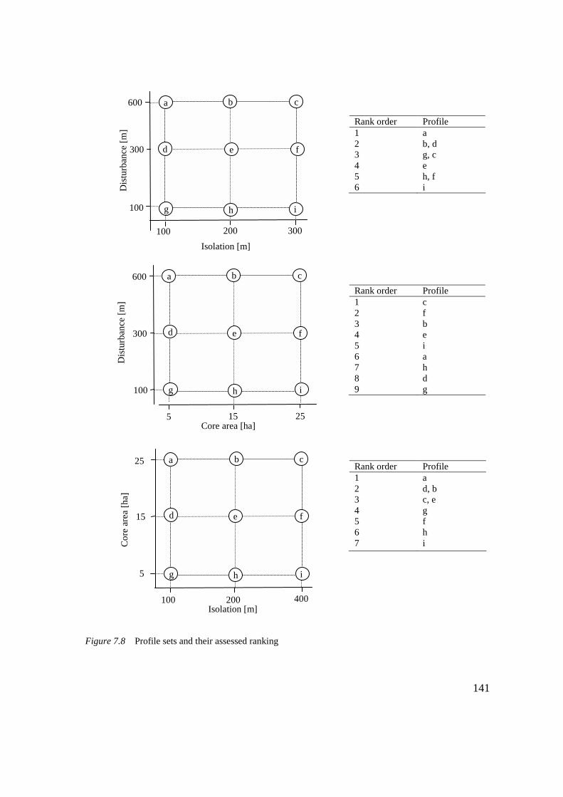
141

Rank order Profile 1 a 2 b, d 3 g, c 4 e 5 h, f 6 i

Rank order Profile 1 c 2 f 3 b 4 e 5 i 6 a 7 h 8 d 9 g

Rank order Profile 1 a 2 d, b 3 c, e 4 g 5 f 6 h 7 i

Figure 7.8 Profile sets and their assessed ranking

b

d

c

e

g

f

h i

a

100 200 300

Isolation [m]

600

100

300

Dis

turb

ance

[m]

b

d

c

e

g

f

h i

a

100 200 400 Isolation [m]

25

5

15

Cor

e ar

ea [h

a]

b

d

c

e

g

f

h i

a

5 15 25 Core area [ha]

600

100

300

Dis

turb

ance

[m]

142

0

0.1

0.2

0.3

0.4

0.5

0.6

0.7

0.8

0.9

1

0 50000 100000 150000 200000 250000 300000 350000 400000Core area [m2]

Value region boundary

Com puted value function

Estim ated value function

0

0.1

0.2

0.3

0.4

0.5

0.6

0.7

0.8

0.9

1

0 100 200 300 400 500 600 700Isolation [m]


Computed value function

Estimated value function

0

0.1

0.2

0.3

0.4

0.5

0.6

0.7

0.8

0.9

1

0 200 400 600 800

Disturbance [m]


Computed value function

Estimated value function

Figure 7.9 The assessed value functions for core area (top), isolation (middle) and disturbance (bottom)

143

7.3.4.2 ASSESSMENT OF ECOSYSTEM VIABILITY VALUES Having defined value functions and weights for the three indicators, it was possible to assess the viability of every ecosystem patch as follows:

3

Vi = Σ (wj * aj) (7.2) j=1

where: Vi = viability value of patch i; wj = weight of the indicator j; aj = value score of the indicator j, calculated using the relevant value function.

As a result, seven viability maps were obtained, showing the viability of the remnant natural ecosystems in the original condition (zero alternative), and in the six alternative scenarios. Figures 7.10 and 7.11 show two examples of them.

Figure 7.10 Ecosystem-viability map of Alternative 0. The legend refers to the viability value of the ecosystem patches. See relevant colour plate

144

Figure 7.11 Ecosystem-viability map of Alternative 6. The legend refers to the viability value of the ecosystem patches. See relevant colour plate

7.3.5 Assessing ecosystem fragmentation As discussed in 4.4.3, the fragmentation impact caused by the six project alternatives was to be assessed in terms of reduction of viability of the natural ecosystems that remain after the construction of the project. For this purpose, each of the six viability maps was compared with the pre-project viability map. This allowed generating the fragmentation-impact maps shown in Figure 7.12. Such maps quantify the reduction in viability (VL, in expression 7.3) expected for each remnant ecosystem patch, due to the presence of the new infrastructure. Only the patches whose viability value is different from the original one are represented, so that the maps highlight the spatial spread of the fragmentation impact of each project alternative. To allow a numerical comparison of the alternatives, each fragmentation-impact map was aggregated into a synthetic impact score. Such a score was computed by multiplying the loss in viability of each remnant ecosystem by its area and by its rarity value (R, see Table 7.5). So, for each alternative i, the fragmentation-impact score EFi was assigned according to the following expression: n

EFi = Σ (VLj * Sj * Rj) (7.3) j=1

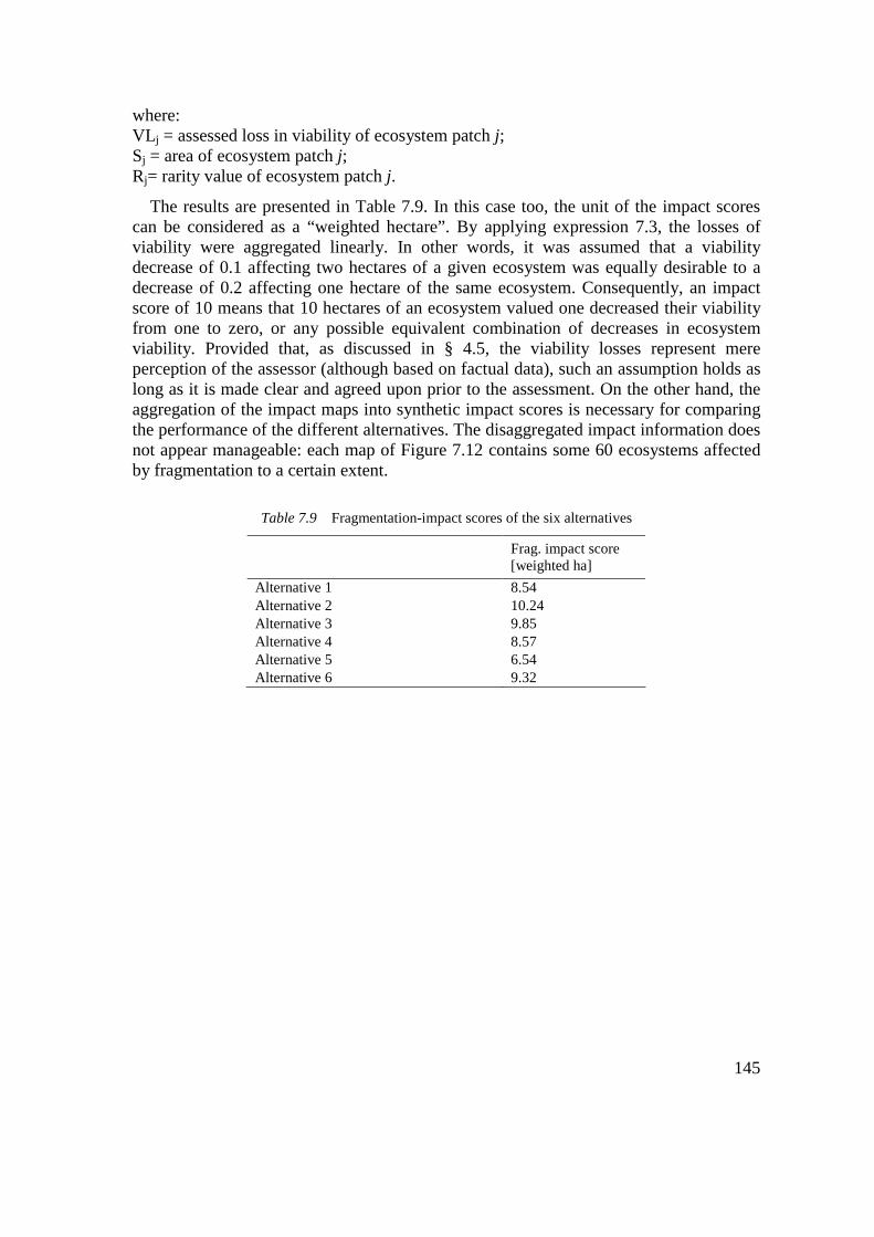
145

where: VLj = assessed loss in viability of ecosystem patch j; Sj = area of ecosystem patch j; Rj= rarity value of ecosystem patch j.

The results are presented in Table 7.9. In this case too, the unit of the impact scores can be considered as a “weighted hectare”. By applying expression 7.3, the losses of viability were aggregated linearly. In other words, it was assumed that a viability decrease of 0.1 affecting two hectares of a given ecosystem was equally desirable to a decrease of 0.2 affecting one hectare of the same ecosystem. Consequently, an impact score of 10 means that 10 hectares of an ecosystem valued one decreased their viability from one to zero, or any possible equivalent combination of decreases in ecosystem viability. Provided that, as discussed in § 4.5, the viability losses represent mere perception of the assessor (although based on factual data), such an assumption holds as long as it is made clear and agreed upon prior to the assessment. On the other hand, the aggregation of the impact maps into synthetic impact scores is necessary for comparing the performance of the different alternatives. The disaggregated impact information does not appear manageable: each map of Figure 7.12 contains some 60 ecosystems affected by fragmentation to a certain extent.

Table 7.9 Fragmentation-impact scores of the six alternatives

Frag. impact score [weighted ha]

Alternative 1 8.54 Alternative 2 10.24 Alternative 3 9.85 Alternative 4 8.57 Alternative 5 6.54 Alternative 6 9.32

146

Figure 7.12 Fragmentation-impact maps of the six alternatives (outlined in black). The values indicate the reduction in viability of the affected ecosystems. See relevant colour plate

Alt.1 Alt.2

Alt.3 Alt.4

Alt.5 Alt.6

147

7.4 Performance of the six alternatives The impact analysis carried out in this chapter has led to the generation of the ecosystem-loss and ecosystem-fragmentation impact scores for each of the six project alternatives (see Tables 7.10). This section comments such results in the light of the main characteristics of the six alignments. A preliminary remark is that, as expected, there is not necessarily a correlation between the two types of impacts caused by the alternatives. For example, Alternative 2 has a rather low impact in terms of ecosystem loss, but the highest impact in terms of ecosystem fragmentation. This underlines the fact that a truly complete analysis of the impacts on ecosystems caused by a road development needs to consider a broader area than the mere road-corridor, so as to fully account for relevant effects, such as fragmentation. Table 7.10 Synthesis of the impact assessment results

Ecosystem-loss impact score [weighted ha]

Ecosystem-fragm. impact score [weighted ha]

Alternative 1 45.43 8.54 Alternative 2 37.22 10.24 Alternative 3 35.92 9.85 Alternative 4 35.41 8.57 Alternative 5 28.10 6.54 Alternative 6 45.79 9.32

Alternative 1 represents the second-to-worst performing layout in terms of direct ecosystem loss. On the contrary, it ranks in the second position according to the ecosystem-fragmentation impact (see Table 7.11). The reason of the intense ecosystem loss resides in the fact that this project alternative is to run right along the Noce River for over 3 km, affecting the highly valuable vegetation that covers its banks (see Figure 7.1). For this same reason the fragmentation impact is relatively low: the track, by running close to the river’s banks, do not interfere with the small ecosystem patches that are scattered around the gorge of La Rocchetta. Moreover, the layout crosses the Avisio River’s delta using an already existing road corridor, and therefore not introducing further disruption between the natural ecosystems (see the relevant fragmentation-impact map in Figure 7.12).

Table 7.11 Performance of Alternative 1

Among the six layouts considered in this study, Alternative 2 is the worst-performing one in terms of ecosystem fragmentation and rank only 4th with respect to direct ecosystem loss (see Table 7.12). This is due to the winding crossing of the La Rocchetta

Ecosystem loss Ecosystem

fragmentation Impact score 45.43 8.54 Position 5th 2nd

148

gorge, as well as to the interference with the La Rupe biotope (see Figure 7.1). The biotope is to be crossed just before the beginning of the longest tunnel section. However, by running along the western side of the Valley, the road avoids to affect the remnant patches of Orno-ostryetum woodland scattered in the proximity of the eastern hilly belt.


Alternative 3 ranks 3rd for what concern the ecosystem-loss impact, and 5th for what concerns the ecosystem-fragmentation impact (see Table 7.13). As a matter of fact, despite the long tunnel sections, the layout is to heavily interfere with the Noce riverside ecosystems, especially in the area surrounding the La Rupe biotope (see Figure 7.1). Moreover, the crossing of the La Rocchetta gorge causes loss and disruption of the remnant natural ecosystems, especially in the vicinity of the entrance of the tunnel. However, the road has a limited impact on the ecosystems within the Non Valley, because the track follows closely the existing infrastructure corridors.


Alternative 4 ranks in a rather high position with respect to either types of impact (see Table 7.14). The track has a limited interference with the Noce River system because it first runs along the western side of the Adige Valley, and then cut through it and crosses the river just south of the town of Mezzolombardo, sparing the ecologically relevant area around the La Rupe biotope. However the track cuts through some of the Orno-ostryetum forest remnants scattered along the eastern side of the Adige Valley (see Figure 7.1). Furthermore, the crossing of the Non Valley is particularly impacting, owing to the winding road layout and the proximity to valuable ecosystems, such as the ones within the La Rocchetta biotope.



fragmentation Impact score 37.22 10.24 Position 4th 6th


fragmentation Impact score 35.92 9.85 Position 3rd 5th


fragmentation Impact score 35.41 8.57 Position 2nd 3rd

149

Alternative 5 is the best-performing one, according to both types of impact (see Table 7.15). Its alignment is similar to the one of Alternative 4 up to the crossing of the Noce River. Consequently, its interference with the Noce River system and its natural vegetation is rather limited. The La Rupe biotope is left undisturbed (see Figure 7.1). Furthermore, analogously to Alternative 3, this alternative has also a relatively low impact on the ecosystems within the Non Valley, because the track follows closely the existing infrastructure corridors. However, the road cuts through some of the remnant woodland patches scattered along the eastern side of the Adige Valley.


Alternative 6 is the most impacting one in terms of direct ecosystem loss and among the most impacting in terms of ecosystem fragmentation (see Table 7.16). From an ecological standpoint, its layout seems to include most of the negative characteristics found in the other alternatives. First of all, the road is to cross the Avisio River’s delta by means of a new viaduct, rather than using or enlarging the existing ones. The road is then to interfere with the remnants of Orno-ostryetum woodland, by crossing the eastern side of the Adige Valley, and with the Noce riverside vegetation, by running along the river for few kilometers (see Figure 7.1). The crossing of the La Rocchetta gorge is also highly impacting, because of the rather short tunnel section. However, the layout spares the ecologically relevant La Rupe biotope.

Table 7.16 The performance of Alternative 6

Concluding, Alternative 5 is the best-performing one for what concerns both the ecosystem-loss and the ecosystem-fragmentation impact. Considering that this alternative has also a rather short tunnel section (see Figure 5.4), it can be concluded that the land corridor through which it was designed appears particularly suitable in terms of effects on natural ecosystems. The dominance of Alternative 5 is the only clear indication that emerges from the analysis of the impact scores. The ranking of the other alternatives cannot be established straightforwardly because they perform differently according to the type of impact. It may actually appear of little relevance to rank the remaining alternatives. However it must be remembered that each disciplinary study (like the Biodiversity Impact Assessment carried out in this research) represents only a piece of the mosaic that form the overall Environmental Impact Statement. In turn, environmental concerns embody only a share of the issues involved in the decision-


fragmentation Impact score 28.10 6.54 Position 1st 1st

Ecosystem loss Ecosystem fragmentation

Impact score 45.79 9.32 Position 6th 4th

150

making concerning a development. Obviously, economic and social analyses play a role too, and their conclusions may be at odds with the results of the environmental assessment. Consequently, the disciplinary studies are to offer as many clues as possible about the significance of the predicted impacts, as well as about the position in the ranking of the different alternatives. Differences between alternatives that appear insignificant at this stage may turn out to be relevant during the overall evaluation. Analogously, alternatives may be left out because unacceptable from some standpoints. Hence, it is important to have as clear a picture as possible of the behaviour of the alternatives throughout the whole ranking. In order to obtain such a complete ranking, the impact assessment needs to include one more step: the aggregation of the impact scores and the formulation of synthetic judgments about the overall performance of each alternative. This is the topic of the next chapter that will dwell in particular on the use of uncertainty analysis to test the stability of the ranking. 7.5 Concluding remarks

This section presents a discussion of the advantages, shortcomings and open issues related to the application of the proposed approach that emerged during the analysis. A particular attention has been given to issues concerning its operationalisation, and therefore its potential role in real-life EIAs. Impact prediction and impact assessment. The approach offers the advantage of forcing the evaluation to follow the typical stages of an EIA, and in particular to clearly separate impact prediction from impact assessment. Even though, from a methodological point of view, it is widely held that predicting impacts is something different than assessing impacts, in practice those two stages are often confused and undertaken simultaneously. This happens in EISs, as well as in the scientific literature, as testified by the review carried out in the first part of the book. Impact prediction and impact assessment rely on different techniques and methodologies. In particular, the use of subjective judgments is part of the impact assessment. However, subjectivity should not be included in the impact prediction. If the two stages are merged together, the resulting impact scores will fail to indicate what has been predicted and how this prediction has been transformed into an assessment. In other words, they will be less transparent. Transparency is fundamental in EIA because it represents, among other things, a pre-requisite to ensure effective public participation. The less transparent an EIS is, the harder it will be for the public to react to it, and provide discussions, critics, revisions, and improvements. Biodiversity levels. As discussed in Chapter 4, it was decided to focus the analysis on the ecosystem level of biodiversity only. Investigating the species level too is to provide a more complete impact assessment. For instance, different ecosystems could have been valued not only for the rarity of their vegetation cover, but also by virtue of the presence of rare or endangered or, anyway, relevant animal and plant species. Unfortunately, such analyses require a considerable amount of information on the distribution of species with a level of spatial detail that is usually unavailable. For instance, for the whole territory of the Autonomous Province of Trento, information on the distribution of endangered and

151

endemic plant species are available only at 10-km spatial resolution (De Marchi 2000, Prosser 2000). On the basis of these data, it is not possible to carry out project-level impact assessments. Additional surveys are required. Such surveys are extremely resource-consuming, and therefore should be limited to the locations where they are actually needed. The results of the impact analysis performed in this study can be used as a filter to highlight those sites worth of further investigations. For example, the fragmentation-impact maps shown in Figure 7.12 provide an indication on the ecosystem patches that are to be particularly affected by the project. Within such patches, species-targeted surveys could be carried out to throw the basis for a more comprehensive impact assessment. Planning phase and EIA The prediction and the assessment of the impacts caused by the different alternatives have been carried out by referring to a general space occupation buffer, estimated from the available information about the project. This information was limited because the project was only in the planning phase. In particular, most technical details, such as the exact width of the paved area, the presence of bridges or viaducts, the location of the road-yard and parking lots, were missing. Such details are fundamental to quantify in a more reliable way the space occupation of the infrastructure. On the other hand, developers are reluctant to finance the design of operational projects when several alternatives are proposed and the final one has not been identified yet. Therefore, this case study can be considered as a likely situation. EIA studies dealing with several alternatives need to expect not be able to count on final blueprints, but rather on designs that are not fully detailed. Even though based on imprecise information, the EIA has the task of identifying the most suitable land corridor through which the project can be designed. Once the least-impacting corridor has been identified, the appointed engineers provide the operational project. At this point, the impact assessment can be refined. This is particularly relevant when the law enforces compensation measures for impacts such as habitat loss. That is, the project’s proponent has to restore elsewhere the same amount of habitat that is to be lost, owing to the construction of the project. An example is represented by the “no-net loss” policy adopted for wetland preservation in the USA, or by the ecosystem restoration that follows road developments in The Netherlands (Cuperus et al. 2001, 1999). Adequate compensations can be proposed only when the project details are known, and consequently the losses can be estimated more precisely. Concluding, the proposed approach for impact assessment is suitable as a preliminary way to identify and suggest the least-impacting alignment. Nevertheless, only the operational project can be used to estimate the final impact figures, and to propose suitable compensation measures, such as habitat restoration. Experts. The assessment of the relevance of the impacts was based on the opinion of an expert in the field of ecological evaluation and ecosystem viability. Consequently, the results are influenced by the expert’s personal perception and judgment. To overcome this inconvenient, a panel of experts can be appointed and consulted. Theoretical and practical issues related to the construction of value functions for expert panels were discussed in Beinat (1997). Resorting to an expert panel, rather than a single expert, is particularly recommended for the most delicate issues and those issues characterised by a high degree of uncertainty. In cases where it is not possible to count on expert panels,

152

an alternative approach consists in including uncertainty ranges into the response of the single expert. This approach was adopted in the present research and will be explored in the next chapter, discussing its benefit in terms of confidence in the evaluation results. EISs and biodiversity values. The approach relies on the evaluation of the significance of the different ecosystem types in terms of biodiversity conservation. This requires the establishment of a “value system” (e.g., the functional curve for rarity shown in Figure 7.5). However, it appears neither advisable nor feasible that each and every EIS generates its own value system to assess rarity or whatever other ecological criterion. This would result in a very heterogeneous assessment for the same object throughout the same region and would complicate the procedure of both compiling the EIS and reviewing it. It appears much more adequate, considering both feasibility and effectiveness, that the planning authorities provide their own standards and its own value systems in the form, for instance, of a Biodiversity Conservation Plan.

154

8 Multicriteria evaluation and uncertainty analysis

8.1 Introduction Impact prediction and assessment form the crucial part of an EIS. Consequently, most of the resources available to carry out the study are invested in surveys, analyses and models that can help to obtain a reliable and complete evaluation of the environmental impacts. However, for the EIS to effectively contribute in decision-making, the impact assessment needs to include one critical step: the formulation of synthetic judgments about the overall performance of each alternative, and the subsequent generation of a suitability ranking of the alternatives. In general the analysis of the impacts, being based upon large and complex enquiries, tends to generate encyclopedic reports, unsuitable for direct evaluation by decision-makers. On the contrary, a synthetic analysis is to provide decision-makers with the essential information on the environmental implications of a project, paving the way to an effective decision process. The term “effective” is here used in the sense that it can rely on all the relevant information, provided in a suitable form. A technique that can be used to support the comparison of alternatives for EIA is Multicriteria Evaluation (see § 4.1.2). This technique has been developed to ease and make as transparent as possible the process of comparing the overall performances of the alternatives proposed as solution to a decision problem. Transparency is a fundamental requisite of this process, especially because there is always some degree of subjective judgment involved. The use of Multicriteria Evaluation (MCE) is growing instrumental in EIA applications to the point that, at least in some countries, it can now be considered as a standard supporting technique (Janssen 2001). Besides the ranking and the evaluation of the overall performance of the different alternatives, it is important for the decision-makers to rely on estimations of the uncertainties affecting the MCE results. As discussed in § 3.3.4, the knowledge of the uncertainties related to the decision process increases the awareness of decision-makers, and better orients their strategy. Moreover, it underlines the most critical data or methodological steps of the analysis. This in turn allows steering additional information acquisition and processing toward where it is actually needed to broaden the scientific basis of the decision. As presented in § 4.1.2, MCE-based approaches for comparative assessment of alternatives typically include a procedural step aimed at checking the reliability of the evaluation results: the sensitivity analysis. This analysis consists in introducing a certain level of uncertainty into the evaluation parameters (e.g., the impact scores) and in verifying the consequences on the results, i.e., on the overall performance of the alternatives and their ranking. Sensitivity analyses clearly offer an added-value to the

155

evaluation, providing the decision-makers with insights on the robustness of the ranking. Robustness refers to the degree to which it is possible to draw clear conclusions on the relative merit of the different alternatives (Beinat et al. 1999). However, the limitation of the sensitivity-analysis approach resides in the fact that the uncertainty ranges are imposed arbitrarily. This reduces the usefulness of the output, because it does not tell decision-makers how realistic such ranges are, and how much they should worry about their effects on the result of the evaluation. Consequently, sensitivity analysis can gain in effectiveness if complemented by a sound uncertainty analysis. The latter should be aimed at identifying meaningful ranges of variation of the impact scores, according to the data and the methodologies that have been used for their computation. In this way, a clear connection between the actual sources of uncertainty (e.g., errors in the database, simplified assumptions) and their effects on the final ranking of the alternatives can be established. This helps decision-makers in increasing their awareness about the degree of confidence associated with the evaluation results. In the light of these considerations, the objective of this chapter is to complement the impact assessment undertaken in Chapter 7 by means of two additional analyses. The first one consists in applying MCE techniques to aggregate the impact scores and obtaining a ranking of the alternatives. The second one consists in studying some of the main uncertainties that affect the computation of the impacts and checking their effects on the evaluation results. In particular, the selected uncertainties affect the following data/actions, as shown in Figure 8.1:

� The ecosystem map; � The space-occupation buffer of the alternatives; � The expert’s assessment of both ecosystem viability and rarity.

The rationale that guided the selection of the uncertainty factors is provided by the following observations:

� They sweep all the three procedural stages of EIA undertaken in this research, namely the baseline study, the impact prediction, and the impact assessment. Consequently, it becomes possible to test the propagation of the uncertainties throughout the whole procedure and to highlight the stages that appear particularly critical. This in turn allows to provide indications on where further resources need to be allocated to improve the reliability and the usefulness of the study;

� They involve three different kinds of uncertainty that are typical of EIA and environmental decision-making in general: uncertainty in the data that are used (i.e., the ecosystem map), uncertainty in the methodologies/models that are adopted (i.e., the use of buffers of a given width to model the space-occupation impact of the roadway), and uncertainty in the expression of values (i.e., the expert’s judgments).

For these reasons, the selected factors are deemed to represent the broad range of uncertainties that need to be dealt with in EIA applications. A comprehensive analysis of all the uncertainties affecting the data and of their propagation throughout the different procedural stages (e.g., GIS operations, such as map overlay) goes beyond the scope of this chapter. The chapter focuses on the contribution to EIA decision-making offered by the combination of uncertainty analysis and sensitivity analysis. In particular, the

156

proposed approach aims at enhancing the analysis and the comparison of different project alternatives, as discussed in Section 4.5.

Figure 8.1 Flow-chart of the impact analysis. The gray boxes indicate the methodological steps and the data whose uncertainty factors will be discussed in this chapter. Rectangles refer to actions, whereas parallelogram to data/knowledge

The chapter is organised as follows. Section 8.2 shows the application of MCE to the case study. Sections 8.3 to 8.5 deal with the uncertainty analyses in the baseline study, the impact prediction and the impact assessment, respectively. Finally, Section 8.6 brings the chapter to a close with some concluding remarks. All the MCE-based procedures have been conducted by programming the required operations with spreadsheets.

Generation of space occupation maps

Ecosystem map

Road layouts



Computation of changes in the spatial

parameters

Expert’s opinion

Expert’s opinion



Computation of ecosystem-loss impact scores


impact scores

BASELINE STUDY

IMPACT PREDICTION

IMPACT ASSESSMENT

Aggregation through MCE and ranking of the

alternatives

157

8.2 Application of MCE to the case study

This section aims at applying an MCE approach to derive a suitability ranking of the six project alternatives. The input data are provided by the results of the impact analysis carried out in Chapter 7. Those results are summarised in the two diagrams of Figure 8.2. In particular, § 8.2.1 deals with the procedural steps of value assessment, prioritisation, and aggregation, whereas § 8.2.2 describes the sensitivity analysis of the ranking. Assessing value functions, prioritising and aggregating require value-based information. In other words, value judgments have to be formulated so to orient the selection of the most adequate value function, weight set, and aggregation method. Hence it is crucial at this stage to involve experts, stakeholders and decision-makers in the analysis to make sure that the results match their perspectives. A thorough treatment of these aspects goes beyond the scope of this chapter, as anticipated in the introduction. Consequently, these procedural steps are undertaken without discussing the rationale that has justified the selection of a particular technique. On the contrary, sensitivity analysis is given particular attention, presenting both its advantages and limitations in terms of how it can support decision-making. This is to underline the link with the uncertainty analysis that will be presented and discussed in the remaining of the chapter.

45.43

37.22

35.92

35.41

28.1

45.79

0 10 20 30 40 50

Alt.1

Alt.2

Alt.3

Alt.4

Alt.5

Alt.6

Habitat-loss impact score [weighted ha]

8.54

10.24

9.85

8.57

6.54

9.32

0 2 4 6 8 10 12

Alt.1

Alt.2

Alt.3

Alt.4

Alt.5

Alt.6

Habitat-fragmentation impact score [weighted ha]

Figure 8.2 Ecosystem-loss and ecosystem-fragmentation impact scores of the six project alternatives

8.2.1 Value functions, weight assignment and aggregation The first step of the evaluation consisted in constructing the impact table that contains the impact scores of the six project alternatives (Table 8.1). The scores were then valued by using the following value function:

S = - r /max + 1 (8.1)

where: S : value score; r : raw score; max: highest raw score of the respective criterion.

158

The use of such a linear function has the following implications: � The same increase of an impact scores is equally valued all over the range of the

possible scores (e.g., an increase in the ecosystem loss from 20 to 30 “weighted hectares” is considered as significant as an increase from 30 to 40);

� The ratio between the value scores of two alternatives is the same as the ratio of their original raw scores;

� The worst possible situation (i.e., the value zero) is represented by the highest impact score among the ones of the alternatives under analysis;

� The best possible situation (i.e., the value one) occurs only if an alternative causes no impact at all.

A linear relationship between the impact scores and the perceived significance of the impacts was considered reasonable, being the impact scores already based on the results of value judgments. The application of the value function lead to the results shown in Table 8.1 and in the diagram of Figure 8.3. As it can be seen, a value of zero is assigned to the highest score for each criterion. It represents the highest impact, and therefore the worst performance. All other scores get a value between zero and one. Table 8.1 Raw impact scores (left-hand columns) and valued impact scores (right-hand columns) of the six alternatives

Alt.1 Alt.2 Alt.3 Alt.4 Alt.5 Alt.6 Ecosystem loss 45.43 0.01 37.22 0.19 35.92 0.22 35.41 0.23 28.10 0.39 45.79 0.00

Ecosystem fragment. 8.54 0.17 10.24 0.00 9.85 0.04 8.57 0.16 6.54 0.36 9.32 0.09

0.01

0.19

0.22

0.23

0.39

0

0.17

0

0.04

0.16

0.36

0.09

0 0.1 0.2 0.3 0.4 0.5

Alt.1

Alt.2

Alt.3

Alt.4

Alt.5

Alt.6

Assessed impact score

Habitat fragmentationHabitat loss

Figure 8.3 Diagram representing the impact table after the value assessment

The following step consists in assigning a weight to each criterion. The weight assignment should reflect the relative importance of the habitat-loss impact with respect to the habitat-fragmentation impact. In particular, weights relate to the change in the overall impact significance that occurs when each of the two impact types is moved from

159

its minimum to its maximum score, all other things being equal. Unfortunately, a pair of weights whose suitability can be supported by analytical and objective data does not exist. Weight assignment is a largely subjective operation. Therefore, it is fundamental to involve the decision-makers to make explicit their value systems with respect to the impacts at stake. Here for simplicity equal weights were assigned to the two impact types. The use of equal weights implies that an ecosystem-loss impact of 45.79 (i.e., the worst situation in terms of ecosystem-loss) is equally bad as an ecosystem-fragmentation impact of 10.24 (i.e., the worst situation in terms of ecosystem fragmentation). The effects of using different weight pairs are discussed later on with the sensitivity analysis. Here the aggregation is performed by the weighted summation method, that leads to the results shown in Figure 8.4. Through weighted summation, each alternative was given an overall score ranging between zero and one. Zero means that the alternative is the worst-performing one in terms of both impacts. One means that the alternative causes no impact at all. This value assignment results in a suitability ranking of the alternatives. As shown in Figure 8.4, Alternative 5 outranks unambiguously all the other ones. Alternative 4 ranks in the second position. Alternative 1, 2, and 3 are characterised by rather similar scores. Finally, Alternative 6 ranks in the last position.

0.09

0.09

0.13

0.19

0.37

0.04

0 0.1 0.2 0.3 0.4

Alt.1

Alt.2

Alt.3

Alt.4

Alt.5

Alt.6

Overall score

Figure 8.4 Overall scores obtained using equal weights

8.2.2 Basic sensitivity analysis The last step of the procedure consisted in testing the sensitivity of the results. In particular, two sensitivity analyses can be performed to verify the effects related to changes in the weights and in the impact scores, respectively. The result of the sensitivity analysis related to changes in the weights is shown in Figure 8.5. The diagram represents the overall score of the six alternatives concomitant with all possible pairs of weights assigned to the two impact types. The scores obtained using a weight of 0.5 for both the impact types are indicated by the dotted line. This representation highlights the reversal points, i.e., the weight values that cause a reversal in the rank order of two alternatives. The reversal points occur whenever the lines of two alternatives meet. For example, a weight of about 0.42 assigned to the ecosystem-loss impact causes a reversal between

160

Alternative 1 and Alternative 3, as shown by the little circle in Figure 8.5. This is because for weight values smaller than 0.42 Alternative 1 outranks Alternative 3, whereas the opposite occurs for values larger than 0.42. This analysis suggests that Alternative 5 ranks stably in the first position regardless the weight values. Alternative 4 ranks in the second position as long as the weight assigned to the ecosystem-loss impact is greater than 0.1. As for the remaining alternatives, if the weight assigned to the ecosystem-loss impact is larger than 0.5 they rank as follows: Alternative 3, Alternative, 2, Alternative 1 and Alternative 6. For weight values smaller than that, rank reversals between these four alternatives occur frequently. It is worth noting that the weight value of 0.5 indicates a rank-reversal value for Alternative 1 and 2 (see the rectangle in Figure 8.5). As a matter of fact, these alternatives scored the same when equal weights were used, as shown in Figure 8.4. This analysis offers the decision-makers a clear picture of the effects related to the use of different weight pairs. Hence, it can contribute to a more efficient weight-assignment, for instance by limiting the arguing to the issues that have an actual influence on the evaluation results. However, as specified in the introduction, issues connected with the weight-assignment procedure do not represent the focus of this chapter and this analysis will not be discussed any further.

Figure 8.5 Diagram of the overall scores versus the weight assigned to the ecosystem-loss impact (see text)

The second sensitivity analysis aims at testing the robustness of the results with respect to changes in the impact scores. A way of performing this consists in imposing perturbations on the impact scores to verify their effect on the overall performance of the alternatives. First of all, it is necessary to identify an uncertainty range for every impact score. Such a range represents the maximum percentage by which we expect the score to deviate from its original value. Afterwards, the overall score of each alternative is calculated a large number of times using a random number generator. In this research, a procedure has been implemented that generates 1,000 random number for each impact score, uniformly distributed within the pre-defined uncertainty ranges. Subsequently, new

Weight of the ecosystem-loss impact

0.2

0.4

0.5

0.6

0.8

1

0.4 -

0.3 -

0.2 -

0.1 -

0 -

Alt.5

Score

Alt.4 Alt.1

Alt.6Alt.3

Alt.2

0.5 -

161

standardised impact scores and new overall scores are computed for each alternative, generating 1,000 separate rankings. The procedure can be run, for instance, using an uncertainty range of 10% for all the impact scores and by keeping all the parameters (e.g., weights, value functions) used in the previous sub-section. The results can be summarised in a frequency table that shows how many times an alternative ranks in every position (see Table 8.2). The values of each row in this table do not necessarily sum up to 1,000 because when two alternatives draw they are given the same ranking position, and the next position is not assigned. Table 8.2 Frequency table obtained using an uncertainty range of 10%

Alt.1 Alt.2 Alt.3 Alt.4 Alt.5 Alt.6 1st 0 0 0 0 1,000 0 2nd 8 10 94 894 0 0 3rd 177 195 498 98 0 26 4th 292 344 265 8 0 91 5th 298 321 127 0 0 234 6th 225 130 16 0 0 649

As in the previous analysis, Alternative 5 ranks stably in the first position. Alternative 4 appears also reasonably stable, holding the second position for nearly the 90% of the rounds. On the contrary, the remainder of the ranking appears rather sensitive to the uncertainty factors that have been introduced into the impact scores. In particular, there is no alternative that occupies the 3rd, 4th and 5th position in at least the 50% of the rounds. These results also offer clues for expressing a preference between Alternative 1 and 2 that, as shown in Figure 8.4, used to score the same. In this case the frequency table shows a slightly better performance of Alternative 2. The above-described sensitivity analyses clearly offer an added-value to the overall evaluation, providing the decision-makers with insights about the robustness of the ranking. The procedure can be repeated using different uncertainty percentages, so as to gain knowledge about the behaviour of the alternatives. This increases the confidence that decision-makers have in the results. However, the limitation of this approach resides in the fact that the uncertainty ranges are arbitrarily imposed on the impact scores. As pointed out in Section 8.1, this reduces the usefulness of the analysis because decision-makers are not provided with indications on the likelihood of such ranges. For overcoming this limitation, a sound uncertainty analysis is to be combined with the sensitivity analysis. This is performed in the following three sections. The aim is to estimate and highlight some of the main uncertainty factors affecting the impact scores, and to study their influence on the performance of the alternatives. Owing to the undisputed dominance of Alternative 5 (see Figure 8.4 and 8.5 and Table 8.2), the analysis focuses on the performance of the other five alternatives. The analysis is broken down into the baseline study, the impact prediction, and the impact assessment.

162

8.3 Uncertainty in the baseline study

The baseline study involves the collection and processing of data on the issues of concern highlighted during the scoping stage of an EIA. Such data represent the starting point for the subsequent impact prediction and impact assessment. Consequently, the completeness and accuracy of the whole impact analysis heavily rely on the quality of the database that has been built during the baseline study. As a matter of fact, all errors and inaccuracies contained in the database will propagate throughout the impact prediction and assessment stages, thus influencing the ultimate results of the analysis. In the case study analysed in this research work, the key-data generated during the baseline study is represented by the map of the natural ecosystems occurring within the study area. This map was used as the basic reference to identify the impacts caused by the six road layouts and to estimate their significance (see Sections 7.2 and 7.3). For this reason, it was decided to focus the uncertainty analysis on this data layer. The ecosystem map was derived by the land-cover map, that in turn was constructed by integrating an existing forest database with the classification obtained from remotely sensed data. The procedure has been described in Chapter 6. Just as every map, this map too is likely to contain misclassifications, i.e., discrepancies between the cover type of a pixel and the actual cover of the portion of the earth’s surface to which that pixel corresponds. In particular, automatic classifications of remotely sensed data are subjected to an array of potential sources of error that range from the overlap of spectral signatures of different classes, to the issue of mixed pixels (Janssen 2000, Richards 1993). The present analysis considers only one of all the possible problematic aspects related to the ecosystem map: the identification of the boundary of the ecosystem patches. This is because the study of all the possible sources of error goes beyond the scope of the present chapter and would easily fill a chapter by itself. Mapping the boundary of the different ecosystem types is critical for two main reasons:

a. The boundary may not be evident on the ground. Many natural features are fuzzy by definition, consequently drawing their boundaries involves some degree of arbitrariness. Different forest types naturally occurring within a watershed, for example, may tend to blend gradually into each other, rather than being sharply separated. This problem has been thoroughly discussed in Burrough and McDonnell (1998);

b. Even if the boundaries appear neat on the ground, as in the case of the edges of agricultural fields, they may just not match with the pixel structure of the relevant image data. The unstated implication of classifying each pixel into a land cover type is that the actual land cover fits nicely into multiples of rectangular spatial units (Fisher 1997). This is obviously not the case in the real world, and as a consequence most of the boundary pixels of every mapping unit are actually mixed pixels, i.e., pixels that contain two or more cover types. This prevents from generating a correct delineation of the boundary of the units.

In the present study this situation is further complicated by the fact that the classification of the land cover was performed by combining remotely sensed data with

163

varying spatial resolutions (i.e., aerial photographs and Landsat TM images). Therefore, even though the output map has the compromise resolution of 15 m, the classification is affected by the 30-m resolution of the TM data. In particular, the ortho-photos were acquired in the visible range, therefore the spectral information concerning the infrared range is provided only by the TM image, and therefore has coarser spatial resolution. This type of problem is common to all classifications based on the combination of multi-source images. In the light of these observations, the identification of the patch boundaries is certainly one of the most critical issues related to the accuracy of the ecosystem map. This issue plays also a major role in the prediction of the space-occupation impact of the different road alternatives. Let us consider the example of Figure 8.6. This illustration represents a sub-window of the ecosystem map overlaid with one of the project layouts. As it can be seen, the layout runs along a strip of riverside vegetation. It is clear that a few-meter shift of the boundary of that ecosystem will result in a considerable increase or decrease in the ecosystem loss caused by the road. Such situations are rather common in the study area, due to the fact that many of the layouts tend to follow stretches of the Noce and Adige rivers at the valley bottoms. Moreover, being the riverside vegetation particularly valuable, even small differences in the land-take of this kind of ecosystem are likely to cause significant changes in the overall impact scores. For these reasons, the uncertainty analysis within the baseline study was focused on the identification of the boundaries of the natural ecosystem patches occurring within the study area. In particular, a classification model based on fuzzy boundaries was adopted, as illustrated in § 8.3.1. The effects of such an analysis on the impact scores of the different alternatives and on their ranking are then discussed in § 8.3.2. Conclusions are drawn in § 8.3.3.

Figure 8.6 The layout of Alternative 1 as a black line superimposed on a sub-window of the ecosystem map. Ecosystems are represented as gray patches

Alternative 1

Riverside vegetation

164

8.3.1 Fuzzy-boundary mapping The concept of “fuzzy sets” was introduced in the 1960s (Zadeh 1965) to surmount the restrictions posed by the Boolean logic. Fuzziness can be seen as “a type of imprecision characterising classes that for various reasons cannot have or do not have sharply defined boundaries” (Burrough and McDonnell 1998). These inexactly defined classes are called fuzzy sets. The inclusion of an element within a fuzzy set is defined by a degree of belonging, which is mathematically expressed by a membership function. Such a function in general ranges between zero and one, with one representing full membership and zero non-membership. The assessment of the membership function of a fuzzy set can rely upon expert knowledge or subjective preference, as well as upon clearly defined uncertainties that have a basis in probability theory (Burrough and McDonnell 1998). In Boolean sets, on the contrary, an element is either included in or excluded from a set, and partial membership is not permitted. Hence, the membership function can only take the value zero or one. The concept of fuzzy sets has received some attention in recent GIS applications such as land suitability analysis, where the inclusion of an element within a class is a matter of interpretation, rather than an unequivocal determination (Metternicht 1996, Banai 1993, Burrough et al. 1992). Let us consider an example. The evaluation of the suitability of a land parcel to grow a given crop may be based, among other criteria, on the soil depth. An approach based on crisp sets consists in setting a threshold value and deciding that the parcel is to be considered “suitable” if its soil is deeper than that value, as shown in Figure 8.7 (a). On the contrary, a fuzzy approach allows defining gradual “shades” of suitability, according to the different soil depths. This can be mathematically represented by a membership function that associates any soil depth to a degree of belonging to the “suitable” class, as shown in Figure 8.7 (b). a b

Figure 8.7 Example of crispy (a) and fuzzy (b) membership functions for soil depth-related suitability

In the example just described, the fuzzy concept has been applied to the classification of the attributes (such as the suitability) of geographical objects. The methods of fuzzy logic can be applied also to the delineation of the boundary of geographical objects. This

20

Soil depth

50

100

150

200

1.0

0.8

0.2

0.5

0.0

MF

Suitable

20

Soil depth

50

100

150

200

1.0

0.8

0.2

0.5

0.0

MF

Suitable

165

means that the boundaries of a polygon can be considered “diffuse”, and consequently be represented by a transition zone rather than by a neat line. The transition zone is described by a membership function that specifies, for each location, the degree of belonging to the polygon according to the distance from the original crisp boundary of the polygon itself. In other words, as explained in Burrough and McDonnell (1998), a membership function can be applied so that those sites that are well within the original boundary receive a membership value of one, those sites inside but near the boundary receive a membership value between 0.5 and one, and those sites outside the boundary receive a membership value below 0.5, concomitant with their distance from the boundary. This type of approach has been adopted in the present study to describe the uncertainty associated with the delineation of the patches in the ecosystem map. 8.3.1.1 FUZZY-BOUNDARY ECOSYSTEM MAP The most critical step in generating a fuzzy-boundary ecosystem map consists in defining an appropriate width for the transition zone, and then a suitable membership function. Such choices should be dictated by the scale of the map and by the available knowledge on the fuzzy phenomenon under consideration. As for the size of the transition zone, a 30-m width was considered suitable because it corresponds to the spatial resolution of the coarser data (i.e., the Landsat TM image) used to generate the ecosystem map. Therefore, it was assumed that the actual boundary could be located within a range of 30 m from the mapped one. Not being able to count on evidences about the uncertainty related to the mapping of the boundaries, and for the sake of simplicity, it was decided to adopt a linear membership function. These considerations lead to the definition of the function shown in Figure 8.8 (a). a b Figure 8.8 The membership function adopted in this study (a) and its effects on a generic patch (b). In (a) the negative values refer to distances from the boundary outward. In (b) the different shades of gray relate to the membership values: the darker the hue, the higher the membership to the patch. The dotted circle represents the original (crisp) boundary

-30

Distance from the crisp boundary

-15

0

15

30

1.0

0.8

0.2

0.5

0.0

MF

30 m 30 m

166

This membership function states the following (see also Figure 8.8 b): � The cells located inside a patch and that have a distance of at least 30 m from

the patch boundaries are considered to belong to the patch; � The cells located outside a patch at a distance of at least 30 m from the patch

boundary are considered not to belong to the patch; � The cells located in between are considered to have a degree of membership to

the patch that varies according to their distance from the boundary. Such a membership is defined by a linear function, so that the cells located on the boundary have a membership value of 0.5.

This implies also that the cells located in the transition area of two or more patches will get two or more membership values, expressing their degree of belonging to each of the patches. The procedure to compute a fuzzy boundary in a raster representation consists in first extracting the boundary of the mapping units (using, for instance, edge-detector filters), and then applying the relevant spread function to assign membership values to the cells located in the transition area. In this application, the operation has been performed using the rarity value as attribute of the different ecosystems, according to the assessment illustrated in § 7.3.3. This means that the pixels falling within the transition zones of two or more patches were assigned a value given by the weighted combination of the values of the relevant patches, as in the following expression: n FRa = ∑ (Ri * MVi) (8.2) i=1

where: FRa= rarity value of the pixel a considering fuzzy boundaries; Ri = rarity value of the ith patch whose transition zone encompasses the pixel a; MVi= membership value of the pixel a with respect to the ith patch. n = number of patches within whose transition zone pixel a falls.

From a computational point of view, the area laying around the ecosystem patches (i.e., the landscape matrix characterised by artificial land-cover types) is considered as a patch with a rarity value equal to zero. In case the pixel does not belong to a transition zone, it just keeps its original rarity value. The construction of the ecosystem-rarity map with fuzzy boundaries was performed by means of a dedicated C++ computer program (C. F. Chung, Spatial Data Analysis Laboratory, Geological Survey of Canada: personal communication). The results are shown in Figure 8.9 for a sub-window of the study area. Figure 8.10 presents an enlargement of a transition zone, to better appreciate the effects of the membership function that has been applied.

167

a b

Figure 8.9 A sub-window of the fuzzy-boundary ecosystem map (a) compared with the crisp boundary map (b) used for the impact analysis described in Chapter 7. The rectangle indicates the enlargement in Figure 8.10

Figure 8.10 An example of transition zone between two adjacent ecosystem patches (the original crisp boundary is represented as dashed line). The rarity values are expressed in gray-levels according to the legend of Figure 8.9

8.3.2 Effects on impact scores and alternative ranking This sub-section illustrates the effects caused by the introduction of fuzziness in the ecosystem boundaries on the overall results of the impact analysis. The procedure followed for assessing fragmentation requires the estimation of viability values, which in turn are based on the assessment of three spatial parameters: ecosystem size, isolation and disturbance. Computing and evaluating such parameters while considering fuzzy ecosystem boundaries appeared extremely cumbersome. On top of this, a similar analysis,

60 m

AB

168

but based on the introduction of fuzziness in the value functions used to assess the three parameter, is presented in § 8.5.2. For these reasons, the effects of introducing fuzziness in the ecosystem map were studied only with respect to the ecosystem-loss impact. This was done following one more time the procedural steps carried out in Chapter 7, as described in Figure 8.11.

Figure 8.11 Flow chart of the procedure. The gray boxes indicate the steps repeated in the fuzzy-boundary sensitivity analysis

The ecosystem-rarity map with fuzzy boundaries was superimposed on the space-occupation maps of the five alternatives described in § 7.2.1. This allowed computing the ecosystem-loss impact scores, according to expression (7.1). Table 8.3 contains the impact scores compared with the ones obtained by using the crisp-boundary ecosystem map (see Figure 8.2). As it can be seen, the differences range from about 0.5 to 2%. These new impact scores were then entered in the impact table and a new MCE session was carried out, by using the same parameters and methods, as w ell as the same scores for the ecosystem-fragmentation impact, as in § 8.2.1. The resulting overall scores of the five alternatives (Alternative 5 was not included owing to its unequivocal first position in


Fuzzy- boundary ecosystem map

Road layouts




parameters

Expert’s opinion

Expert’s opinion




scores


impact scores


alternatives

BASELINE STUDY

IMPACT PREDICTION

IMPACT ASSESSMENT

169

the ranking) are shown in Figure 8.12 and compared with the scores obtained during the original analysis. As in that analysis, the best-performing alternative is still Alternative 4 and the second-to-best Alternative 3. However, Alternative 1 and 2 appear now separated and Alternative 6 approaches Alternative 2. Therefore, even though the use of the fuzzy-boundary ecosystem map did not cause any rank reversal, it induced some changes in the relative merits of the different alternatives, especially within the lower part of the ranking. It is worth noting that the approach followed did not change the overall value of each ecosystem patch, but only redistributed it. In particular, the values were assigned in a more gradual way, by smoothing the edges between different mapping units. As a consequence, the alternatives are likely to cause more impact in some locations, but less impact somewhere else. For this reason, a sort of compensation in the ecosystem-loss impact scores is to be expected. As a matter of fact, the differences are only in the order of 1-2 %. On the other hand, the analysis could have highlighted critical situations, such as alternatives whose impact scores changed remarkably when using the fuzzy-boundary ecosystem map. This would have indicated a high sensitivity to eventual errors related to the ecosystem mapping. The analysis was useful in suggesting that there appear not to be such a “sensitive” situation, in which a few-meter shift in a particularly valuable ecosystem upsets the overall impact score of some of the alternatives. Table 8.3 Impact scores computed with fuzzy and crisp ecosystem boundaries

Ecosystem-loss impact scores

Crisp boundaries [weighted ha]

Fuzzy boundaries [weighted ha]

Difference in %

Alternative 1 45.43 46.22 + 1.73 Alternative 2 37.22 37.01 - 0.56 Alternative 3 35.92 35.32 -1.67 Alternative 4 35.41 36.12 +2.00 Alternative 6 45.79 44.90 -1.94

0.08

0.10

0.14

0.19

0.06

0.09

0.09

0.13

0.19

0.04

0 0.05 0.1 0.15 0.2

Alt.1

Alt.2

Alt.3

Alt.4

Alt.6

Overall score

Crisp boundariesFuzzy boundaries

Figure 8.12 Comparison between the overall scores obtained using the fuzzy-boundary and the crisp-boundary ecosystem maps

170

8.3.3 Discussion This section tested the robustness of the impact scores and of the subsequent alternative ranking against a specific source of uncertainty: the fuzziness of the mapping-unit boundary in the ecosystem map. It represents a sensitivity analysis in which the changes in the evaluation parameters are not assigned arbitrarily, but derive from the study of the actual uncertainties affecting the parameters themselves. This analysis could be pushed further to involve a more comprehensive evaluation of the accuracy and reliability of the ecosystem map. The membership function, for instance, could vary according to the unit type, rather than being homogeneous all over the map. Some boundaries (e.g., forest/agriculture) are likely to be sharper than other (forest/grassland), or are likely to be better classified than others (e.g., because of the contrast between the spectral signature of the relevant classes). Analogously, some cover classes are likely to be classified more successfully than others. All this information can be used to carry out an in-depth error analysis on the ecosystem map. This in turn would provide more reliable variability ranges of the parameters to be input in the sensitivity analysis. It goes beyond the scope of this chapter to perform further investigations on the accuracy of the ecosystem map. The main objective of this section, as well as of the following ones, is to exemplify how a framework can be set in which the results of the uncertainty analysis performed on relevant data/methods can accompany the different stages of an EIS so to eventually play a role into the final output of the study to be provided to decision-makers. However, it is worth stressing that the assessment of the accuracy of land cover classifications has been largely addressed in the remote-sensing literature of the last decade (De Groeve and Lowell 2001, Pugh and Congalton 2001, Heuvelink and Lemmens 2000, Stein et al. 1999, Janssen and Wel 1994). Consequently, impact analysts are likely to be provided more and more often not just with the data layers, but also with indications on their accuracy. Such indications must be taken into consideration during the impact analysis. 8.4 Uncertainty in the impact prediction

Uncertainty is an unavoidable component of each prediction (De Jongh 1988). This is because impact predictions rely on models of the environment that need to have simplified assumptions, and consequently cannot reproduce exactly what happens in reality. In this study, the key-operation during the impact-prediction stage consisted in overlaying the image of the expected space occupation of the different project alternatives with the map image representing the distribution of the natural ecosystems within the study area. This allowed generating landscape scenarios that were subsequently used to compute the ecosystem losses, as well as the changes in the spatial parameters of each patch. The critical stage of this procedure is represented by the identification of a suitable space occupation buffer, as discussed in § 7.2.1. The width of such a buffer was estimated by considering the available information about the project, and by referring to analogous case studies found in the literature. However, the choice of the buffer width necessarily involved some degree of arbitrariness. This is due to the

171

unavailability of the technical details of the project (e.g., presence of bridges or viaducts, location of the road-yard, etc.), as well as to the lack of knowledge about the actual spread of the impacts outward from the paved area. On the other hand, even small differences in what is assumed to be the width of the area occupied may produce, over the whole length of the track, significant changes in the predicted impact. In the light of these observations, it becomes meaningful to study the sensitivity of the final impact scores with respect to variations in the width of the selected space-occupation buffer. This has been accomplished by using space-occupation “ranges” and by studying their effect on the ecosystem-loss impact scores. This analysis is described in § 8.4.1 and the relevant conclusions are drawn in § 8.4.2.

8.4.1 Considering space-occupation ranges The actual width of the space-occupation buffer of each alternative is difficult to estimate. Moreover, such a width is subjected to variations along the track, concomitant to changes in the topography (Heinrich and Hergt 1996, Lanzavecchia 1986), as well as in the technical characteristics of the project. A possible approach to account for this consists in deciding that, not being able to count on the engineering details of the projects, it is more meaningful to provide impact ranges, rather than sharp impact scores. The end points of such ranges are computed considering the minimum and the maximum expected space occupation widths. In other words, it is assumed that, at every location of the road track, the effect extends on both sides between a minimum and a maximum distance. The obtained impact ranges are then treated statistically to provide an evaluation of the performance of the alternatives in form of frequency tables. The procedure is akin to the sensitivity analysis on the impact scores performed in § 8.2.2. However, the philosophy of this approach is different because the perturbations are not imposed directly on the impact scores, but on the data and methods that were used to generate such scores. The original space occupation buffer had a width of 120 m. In this analysis it was considered to vary first between 110 and 130 m. For each of these extreme values the ecosystem-loss impact of the five alternatives was computed, following the procedure illustrated in Figure 8.13. The results are shown in Table 8.4. As it can be seen, shifting the buffer width of ± 10 m induces a variation in the impact scores in the order of 5-10%. In particular, Alternative 6 appears rather sensitive, whereas Alternative 2 is the most stable one. It is interesting to notice that the percentages of variation of the impact scores are generally not “symmetric.” For example, the score of Alternative 3 varies by almost 11% if the buffer is 10 m wider, but only by 4.5% is the buffer is 10 m narrower. These results provide indications on the distribution of the ecological values within the land corridors through which the alternatives have been designed. The last step of the analysis consisted in obtaining a large number of points to generate statistically relevant results. For this purpose, 1,000 random numbers for each impact score were generated. They were uniformly distributed between the variation ranges previously obtained. Subsequently, the MCE was repeated, originating 1,000 separated rankings of the alternatives. The results are summarised in Table 8.5. This frequency table shows that the first two positions are firmly held by Alternative 4 and 3,

172

respectively. It also indicates that Alternative 2 tends to outrank Alternative 1, offering a solution to the draw present in the original analysis (see Figure 8.4).

Figure 8.13 Flow-chart of the procedure. The gray boxes indicate the steps repeated in the fuzzy space-occupation sensitivity analysis

Table 8.4 Impact scores computed by shifting the buffer width of ± 10 m

Ecosystem-loss impact scores

120-m buffer [weighted ha]

110-m buffer [weighted ha]

Difference (%) 130-m buffer [weighted ha]

Difference (%)

Alternative 1 45.43 41.86 -7.85 48.90 +7.63 Alternative 2 37.22 34.33 -7.76 39.28 +5.53 Alternative 3 35.92 32.03 -10.82 37.57 +4.59 Alternative 4 35.41 32.17 -9.14 37.40 +5.61 Alternative 6 45.79 40.78 -10.94 48.93 +6.85


Fuzzy- boundary ecosystem map

Road layouts




parameters

Expert’s opinion

Expert’s opinion




scores


impact scores


alternatives

BASELINE STUDY

IMPACT PREDICTION

IMPACT ASSESSMENT

173

Table 8.5 Frequency table obtained using the 110-130 m buffer range

Alt.1 Alt.2 Alt.3 Alt.4 Alt.6 1st 0 0 0 1,000 0 2nd 32 42 926 0 0 3rd 303 600 67 0 30 4th 509 314 7 0 170 5th 156 44 0 0 800

A second analysis was run considering a wider range of the space-occupation buffer: between 100 and 140 m. Table 8.6 shows the resulting impact scores and Table 8.7 the rank frequencies obtained. As it can be seen, shifting the buffer of ± 20 m causes a variation in the impact scores of about ± 20%. As in the previous analysis, Alternative 2 is the most stable one. The frequency table highlights a number of possible rank reversals. In particular, only the first, second and sixth positions are held by the same alternative (i.e., by Alternative 5, 4, and 6 respectively) in more than 50% of the rounds. The remaining ranks, and especially the forth one, appear highly unstable and hard to assign to one single alternative. Table 8.6 Impact scores computed by shifting the buffer width of ± 20 m

Ecosystem-loss impact scores 120-m buffer

[weighted ha] 100-m buffer [weighted ha]

Difference (%) 140-m buffer [weighted ha]

Difference (%)

Alt. 1 45.43 37.04 -18.46 54.54 +20.05 Alt. 2 37.22 31.57 -15.18 43.1 +15.79 Alt. 3 35.92 30.09 -16.23 42.03 +17.01 Alt. 4 35.41 29.7 -16.12 41.66 +17.65 Alt. 6 45.79 36.59 -20.09 55.48 +21.16 Table 8.7 Frequency table obtained using the 100-140 m buffer range

Alt.1 Alt.2 Alt.3 Alt.4 Alt.6 1st 54 28 114 802 2 2nd 195 186 407 156 56 3rd 221 312 279 39 149 4th 292 337 168 3 200 5th 238 137 32 0 593

8.4.2 Discussion This section aimed at creeping perturbations at the impact-prediction level and tracking their effects throughout the impact-analysis procedure to the ranking of the alternative (see Figure 8.13). The perturbations factors derived from a specific uncertainty related to the size of the space-occupation buffer of each alternative. This resulted in a sensitivity analysis driven by the actual uncertainty related to the adopted procedure. The uncertainty analysis performed in this section could be further extended, by considering

174

different membership functions or different variation ranges for the space-occupation buffers. Statistical distributions different from the uniform distribution (such as the normal one) could also be used for generating the random numbers. However, it seems that further evidences on the road effects are needed to justify the selection of one specific method. This section mainly aimed at stressing that, being the space occupation hard to define in a reliable way, it is worth to make explicit this vagueness during the impact analysis and to test its effects on the final results. One conclusive remark is that this section undertook a type of uncertainty related to the method (how should we predict the space occupation impact?), whereas the previous section dealt with uncertainty related to the data (how good is the map that we are using for the impact analysis?). Finally, the next section discusses another fundamental type of uncertainty that affects EIA: the value-based uncertainty, i.e., the uncertainty connected with the formulation of the value judgments and preferences upon which the estimation of the significance of the impacts is based. 8.5 Uncertainty in the impact assessment

The assessment of environmental impacts is based upon value judgments, and therefore it involves subjectivity by definition. This makes this stage particularly prone to criticisms by opponents and open to arguments of every sort. Sensitivity analysis is important to help in representing the consequences of each assessment, so as to mainstream discussions and further analyses (e.g., broadening the panel of experts) toward the issues that are bound to play a significant role for the problem under investigation. This section considers the sensitivity of the results with respect to changes in the expert’s assessment. In particular, the analysis is based on the use of indications of value coarser than the sharp value functions originally provided by the expert. The impact analysis performed in Chapter 7 turned to the expert’s opinion in two explicit stages: the evaluation of ecosystem rarity, and the evaluation of ecosystem viability. As shown in Figure 8.14, the first assessment has an influence on the computation of both the ecosystem-loss and ecosystem-fragmentation impact. On the contrary, the second assessment affects only the ecosystem-fragmentation impact scores. The uncertainty analyses with respect to these two assessments are discussed next.

175

Figure 8.14 Flow-chart of the procedure. The gray boxes indicate the steps repeated in the sensitivity analysis related to the uncertainty in the rarity values

8.5.1 Uncertainty in the assessment of rarity values The assessment of the rarity value of the different ecosystems was provided by an expert through the functional curve shown in Figure 7.5. Such rarity values were then employed to compute the scores for both the ecosystem-loss and the ecosystem-fragmentation impact, applying expressions (7.1) and (7.3), respectively. This sub-section aims at testing the sensitivity of the impact scores and of the subsequent alternative ranking with respect to changes in the assignment of the rarity values. In particular, it was decided to “shake” those values within the ranges provided by the expert in the first stage of the assessment (see Figure 7.5 and Table 7.4). The rationale behind this decision was provided by the following considerations. The expert was selected because he was thought capable of providing meaningful judgments. Therefore, it does not make sense to test the sensitivity of the results using values that completely disregard his opinion. On the other hand, the expert himself showed some hesitation in assessing the sharp values, whereas he was rather confident about the value ranges. Consequently, it appears informative to see the effect on the results of the analysis caused by the fluctuation of the rarity values within the ranges delimited by the end points provided by the expert. This is obtained by repeating the procedural steps highlighted in Figure 8.14. The curves connecting the minimum and the maximum values were used to re-compute the impact scores for both ecosystem loss and ecosystem fragmentation. The results are shown in Table 8.8 and 8.9, respectively. These results offer an impression of the sensitivity of the impact scores to changes in the rarity values. For example, an interesting remark is that the best-performing Alternative 4 appears also as the less stable in terms of ecosystem-loss impact.



parameters

Expert’s opinion

Expert’s opinion




scores


impact scores


alternatives

IMPACT PREDICTION

IMPACT ASSESSMENT

176

Table 8.8 Ecosystem-loss impact scores computed using sharp, minimum, and maximum rarity values

Ecosystem-loss impact scores Sharp values Min values Difference (%) Max values Difference (%) Alternative 1 45.43 42.09 -7.35 49.01 7.88 Alternative 2 37.22 34.33 -7.76 40.44 8.65 Alternative 3 35.92 32.55 -9.38 39.26 9.29 Alternative 4 35.41 31.22 -11.83 39 10.13 Alternative 6 45.79 41.15 -10.13 49.25 7.55 Table 8.9 Ecosystem-fragmentation impact scores computed using sharp, minimum, and maximum rarity values

Ecosystem-fragmentation impact scores Sharp values Min values Difference (%) Max values Difference (%) Alternative 1 8.54 8.10 -5.15 8.98 5.15 Alternative 2 10.24 9.05 -11.62 10.72 4.68 Alternative 3 9.85 9.30 -5.58 10.12 2.74 Alternative 4 8.57 7.91 -7.70 8.95 4.43 Alternative 6 9.32 8.75 -6.11 10.11 8.47 The ranges obtained were then used to generate 1,000 separate alternative rankings. The resulting frequency values are shown in Table 8.10. As it can be seen, Alternative 4 occupies the first position in over the 95% of the rounds. On the contrary, the remainder of the ranking is characterised by a rather high instability as several reversals occur. Alternative 2 and Alternative 1 scored the same in the original analysis. Here Alternative 2 seems to perform better than Alternative 1, confirming the results obtained by introducing uncertainty at the impact-prediction level (compare with Tables 8.5 and 8.7). This can be deduced by comparing the frequency with which the two alternatives occupy the different position of the ranking. Table 8.10 Frequency table

Alt.1 Alt.2 Alt.3 Alt.4 Alt.6 1st 0 8 34 958 0 2nd 50 232 672 41 5 3rd 243 476 233 1 47 4th 536 229 60 0 175 5th 171 55 1 0 773

8.5.2 Uncertainty in the assessment of viability values The other stage in which expert’s opinion was input to the impact analysis was the assessment of viability values, which represented the basis for the computation of the fragmentation-impact scores. The viability of each ecosystem patch was computed through the weighted summation of the values assigned to three indicators: size, isolation, and disturbance. Therefore, for each indicator the expert was asked to assess both a value

177

function and a weight. The current analysis aims at testing the robustness of the results when uncertainties are crept into such assessments. In particular, it aims at exploring the effects of changing the assessed parameters in a limited surrounding of their original value. For what concerns the value functions, such “limited surrounding” was inferred by the value regions drawn by the expert in the very first stage of the assessment (see Figure 7.7). As for the weights, arbitrary percentage ranges were set. The analysis consisted in generating for each ecosystem a high number of possible viability values. Each viability value was computed using randomly generated indicator values and weights. The random values were statistically distributed within the value region of the relevant indicator. The weights were distributed around the value originally selected by the expert. The operation was performed by a dedicated C++ computer program (C. F. Chung, personal communication) that allowed choosing the desired statistical distribution for each parameter. The output of the program consists in a table that summarises for each ecosystem patch the statistical parameters of its viability value, such as median, average, and standard deviation. For the purposes of the current analysis, a uniform distribution was used and a variation of ± 20% was permitted in the weight values. The resulting average viability values were used to compute the fragmentation-impact scores and to generate a new alternative ranking, following the procedure indicated in Figure 8.15. The results are shown in Table 8.11 and Figure 8.16. As indicated by Table 8.11, the uncertainty introduced in the viability values causes variations ranging between –5% and + 10% in the fragmentation-impact scores. This results in quite some change in the overall score of the different alternatives, and in particular of Alternative 2 and 4 (see Figure 8.16). However, the only rank reversal occurred in the second position, now hold by Alternative 2.

Figure 8.15 Flow chart of the procedure. The gray boxes indicate the steps repeated in the sensitivity analysis related to uncertainty in the viability values



parameters

Expert’s opinion

Expert’s opinion




scores

Computation of ecosystem-

fragmentation impact

Aggregation and ranking of the alternatives

IMPACT PREDICTION

IMPACT ASSESSMENT

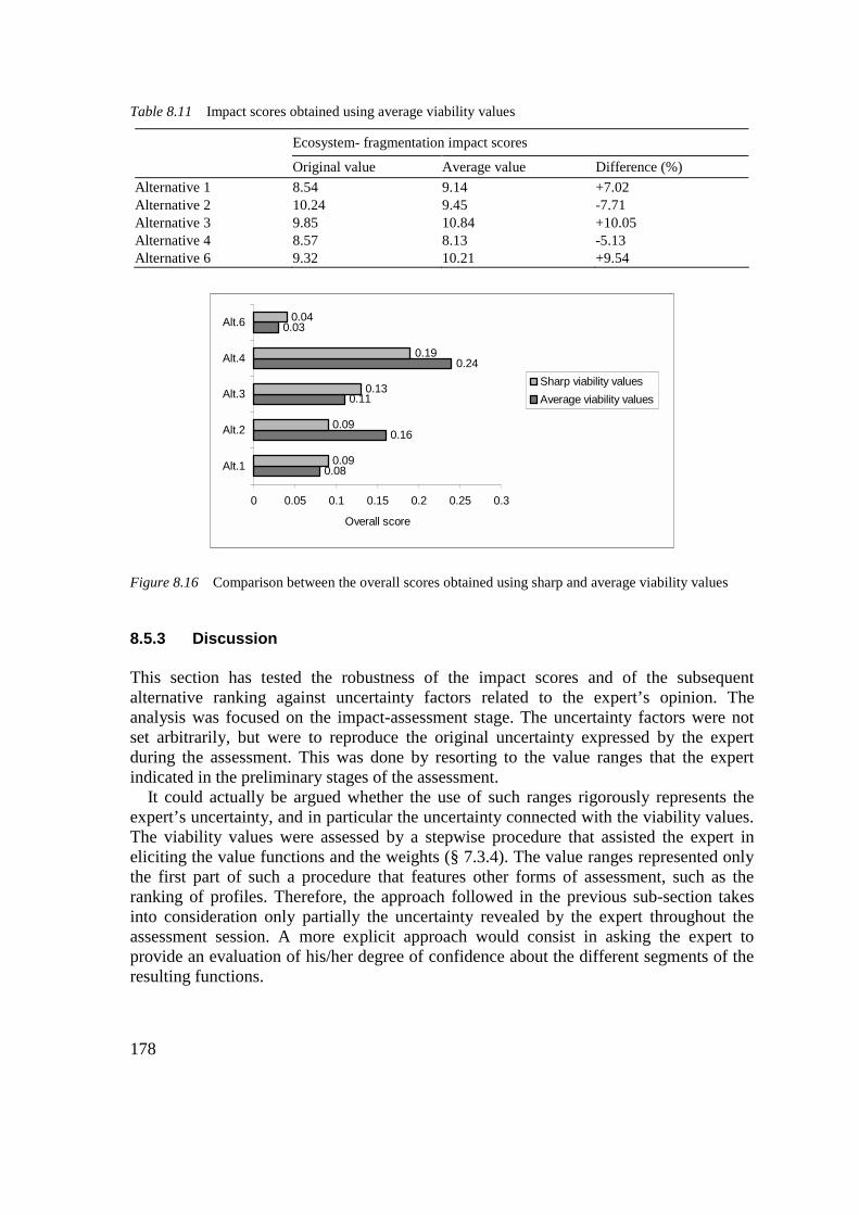
178

Table 8.11 Impact scores obtained using average viability values

Ecosystem- fragmentation impact scores Original value Average value Difference (%) Alternative 1 8.54 9.14 +7.02 Alternative 2 10.24 9.45 -7.71 Alternative 3 9.85 10.84 +10.05 Alternative 4 8.57 8.13 -5.13 Alternative 6 9.32 10.21 +9.54

0.08

0.16

0.11

0.24

0.03

0.09

0.09

0.13

0.19

0.04

0 0.05 0.1 0.15 0.2 0.25 0.3

Alt.1

Alt.2

Alt.3

Alt.4

Alt.6

Overall score

Sharp viability valuesAverage viability values

Figure 8.16 Comparison between the overall scores obtained using sharp and average viability values

8.5.3 Discussion This section has tested the robustness of the impact scores and of the subsequent alternative ranking against uncertainty factors related to the expert’s opinion. The analysis was focused on the impact-assessment stage. The uncertainty factors were not set arbitrarily, but were to reproduce the original uncertainty expressed by the expert during the assessment. This was done by resorting to the value ranges that the expert indicated in the preliminary stages of the assessment. It could actually be argued whether the use of such ranges rigorously represents the expert’s uncertainty, and in particular the uncertainty connected with the viability values. The viability values were assessed by a stepwise procedure that assisted the expert in eliciting the value functions and the weights (§ 7.3.4). The value ranges represented only the first part of such a procedure that features other forms of assessment, such as the ranking of profiles. Therefore, the approach followed in the previous sub-section takes into consideration only partially the uncertainty revealed by the expert throughout the assessment session. A more explicit approach would consist in asking the expert to provide an evaluation of his/her degree of confidence about the different segments of the resulting functions.

179

However, the main scope of this section is to show the applicability of a method that accounts for value-based uncertainty and tracks its effects to the impact assessment results. Uncertainty is introduced at the stage in which the value judgments are formulated, rather than in the final impact scores directly. This causes the different alternatives to react in different ways, revealing their intrinsic sensitivity to the specific value-based uncertainty. This intrinsic sensitivity depends upon the degree of uncertainty associated with the viability and rarity values of the ecosystems that the alternative is to impact. The main advantage, as in the previous two sections, is that decision-makers are provided with clear connections between the sources of uncertainty and their effects on the merit and ranking of the alternatives. 8.6 Concluding remarks

This chapter complemented the impact assessment of the Trento-Rocchetta road project performed in Chapter 7. First of all it proposed a framework based on MCE techniques for aggregating the impact scores and obtaining a suitability ranking of the alternatives. Secondly, it assessed the sensitivity of the results obtained with respect to possible changes in the input of the analysis. The estimation of these changes was derived from a specific study of some of the main uncertainties that affect the different stages of the procedure applied in Chapter 7. The overall objective of this chapter was to provide decision-makers with as comprehensive an information as possible about the performance of the different alternatives. This last section presents some considerations on the results of the case study, the added-value provided by the approach proposed, and the problems related to its operationalisation. On the case-study results. Alternative 5 is by far the best-performing one, i.e., the one that causes the least impact on ecosystems. Such an alternative is to cross the eastern margin of the Adige Valley and managed to spare most of the sites relevant for biodiversity conservation. As for the remaining alternatives, all the uncertainty analysis revealed that Alternative 4 holds the second position rather firmly. Alternative 3 tends to rank in the third position, though a reversal often occur with Alternative 2. Alternative 2 performs generally better than Alternative 1. Finally, Alternative 6 is the last one, though its performance is often very close to the one of Alternative 1. On the added-value for decision-making (1). The results of the analyses performed in this chapter can be used to increase the awareness of the decision-makers about the merit of the different alternatives, and consequently to better orients their strategy. Mere sensitivity analyses provide general indications on the stability of the ranking, but do not tell decision-makers anything about the meaningfulness of the variability ranges selected and of the results obtained. For example, the sensitivity analysis carried out in § 8.2.2 sets the variability range of the impact scores to 10%. This leaves the decision-makers with unanswered questions such as the following ones:

� Is it reasonable to expect a variation of 10% in the impact scores? � Is it reasonable to apply the same variation range to all the impact scores?

180

� Is it reasonable to consider a variation in both directions (i.e., plus and minus 10%) equally probable?

Consequently, the resulting frequency table (see Table 8.2) is hard to interpret. For example, say that we want to identify the alternative that ranks in the second position. The frequency table suggests that Alternative 4 occupies such a position in nearly the 90% of the rounds. However, Alternative 3 also ranked in that position in about the 10% of the rounds. Decision-makers are not told how much they should worry about this 10%, and consequently how confident they can be in assigning the second position to Alternative 4. On the contrary, the approach proposed in this chapter provides a clear connection between the actual sources of uncertainty and their effects on the stability of the ranking. Therefore, the sensitivity analysis explicitly refers to a problematic aspect of the procedure that, at least in principle, can be deepened and improved whenever required to support the decision-making. For example, the frequency table obtained by considering space-occupation ranges (see Table 8.7) shows that Alternative 4 ranks in the first position in about 80% of the cases. The decision-makers are told that this is due to the fact that the actual space occupation of the project cannot be sharply predicted. Consequently, they gain insights on how to interpret the results and they become aware of the risk related to, for instance, selecting Alternative 4. In cases in which they may want to rely on a more stable ranking, the results of the analyses suggest in which directions further efforts must be pointed. This last issue is discussed next. On the added-value for decision-making (2). The analysis performed in this chapter is useful to highlight the most critical data or methodological steps. This in turn allows steering additional information acquisition and processing toward where it is actually needed to support the decision. For example, the selection of the width of the space occupation buffer proved to have an influence on the relative performance of the alternatives (see Tables 8.5 and 8.7). On the contrary, the fuzzy-boundary ecosystem mapping did not introduce significant changes in the impact scores (see Table 8.3). Therefore, the first type of analysis is worth further investigations, especially so because the selection of the buffer width is hard to be justified soundly. Such investigations may be targeted only at the road corridors that appear more sensitive, such as the ones of Alternative 6 and Alternative 1. Let us consider another example. If the decision problem narrows down to choosing between Alternative 3 and Alternative 2 (for instance because Alternatives 5 and 4 appeared not suitable from other standpoints) the analyses conducted in this chapter suggest to pay particular attention to the assignment of the viability scores. As shown in Figure 8.16, small changes in such scores caused a reversal in the ranking of these two alternatives. Consequently, it may be worthwhile to invest more resources in the generation of the value functions used to assess viability. New evaluation sessions could be run to define the functions with more detail (e.g., by using more control points) or another expert could be involved in the assessment to obtain a second opinion. Indications on where to invest further resources are vital in EIAs, which typically are carried out under time and budget constraints and have to deal with potentially endless data collections, analyses and evaluations. On the added-value for decision-making (3). The third contribution to decision-making provided by the analyses discussed in this chapter consists in the increased

181

honesty about the limits of understanding and assessing of ecological impacts. It means that difficulties and uncertainties are not concealed, but made explicit. Moreover, their effects on the performance of the alternatives are accounted for, providing more credible results. This smoothes the decision-making process because it helps in preventing from last-minute objections and arguments. For example, sharp boundaries between natural ecosystems are rarely found in nature. Showing that this fact was considered, and providing the results obtained when fuzzy boundaries are used, increases the defensibility of the assessment. The same applies to critical issues, such as the width of the space-occupation buffer or the assignment of rarity values. One final note. Most of the analyses exemplified in this chapter are fairly simple from both a conceptual and a computational standpoint. In principle, it appears realistic to consider them applicable on a routine basis to complement the impact analysis within an EIS. However, there is one limitation in current EIS practice that is bound to affect the operationalisation of the approach proposed here. This limitation concerns the actors involved in the EIS. This approach relies on the full co-operation and information sharing within the work group that is appointed to perform the EIS. In particular, the specialist in charge of the aggregation of the results (e.g., through the MCE) needs to be fully aware of the procedural steps that have lead to the generation of the impact scores and of the uncertainty that affects such steps. In other words, he/she needs to closely interact with the specialists (ecologist, geologist, etc.) that carried out every single disciplinary study. The impression from reviewing an EIS is that often this is not the case and the different tasks are split rather neatly among the work groups. This is common also to most research papers dealing with EIA issues: either they focus on the prediction and assessment of the impact on some environmental components, or in the subsequent aggregation of the results and decision-making. The former group deepens problems such as data collection and impact modeling, whereas the latter group typically starts the analysis from an impact table and discusses issues connected with weighting techniques, stakeholder analysis, group decisions, etc. This division of tasks and approaches reduces the feedback between the impact analysis and the MCE. Such a feedback contributes to enhance the overall support to decision-making, as underlined by the approach proposed in this chapter.

182

9 Summary and conclusions 9.1 Introduction

The procedure of EIA is to promote the consideration of environmental concerns during the decision-making related to the approval of new development activities. Among these concerns are ecological issues, such as the loss in the value and the viability of natural ecosystems and species. Accounting for such issues is critical for attaining sustainable development objectives, which have recently emerged as the main frame to guide in future environmental management. Ecological evaluation aims at developing and applying methodologies to assess the relevance of an area for nature conservation. As such, it is to support the assessment of the ecological impact of a proposed project, by providing guidance on how to describe the ecological features within the area affected, how to value them, and how to predict the value losses caused by the project activities. However, limited progress has been made by the scientific research to adapt the existing frameworks for ecological evaluation specifically to the evolving procedure of EIA. As a result, the assessment of the ecological component within EIA tends to be flawed. Ecological research needs to improve the guidance provided to impact analyses, so as to encourage good practice within EISs, and to eventually strengthen the consideration of ecological issues in the decision-making for new developments. To this end, the application of ecological evaluation to EIA was chosen as the subject of this study. In particular, the overall objective of the study was to expand the use of ecological evaluation within EISs. The study has focused on one specific target of ecological evaluations, i.e., biodiversity conservation, and on one specific type of projects, i.e., linear infrastructures, and roads in particular. This overall objective was reached by pursuing the following intermediate objectives:

1. To illustrate the role played by ecological evaluation within the procedure of EIA and to highlight the key-issues that need to be addressed by research in this field (Chapter 2);

2. To provide the rationale for the selection of the specific research topic, i.e., BIA of road projects, and to identify the main limitations that affect the current applications in such a topic (Chapter 3);

3. To develop a methodological approach for BIA of road projects so as to provide solutions to the limitations that emerged during the literature review (Chapter 4);

4. To test the applicability of the proposed approach to a case study and to discuss issues related to its operationalisation in real contexts (Chapters 5-8).

Through this sequence of steps it was possible to provide a contribution to the current practice of BIA of road developments. In particular, three stages of EIA (baseline study,

183

impact prediction, and impact assessment) and two types of impact (ecosystem loss and ecosystem fragmentation) have been addressed. The next four sections describe how each of the objectives listed above has been reached. Section 9.6 discusses some thoughts on possible future developments of this study. 9.2 Ecological evaluation for EIA

Ecological evaluation is the process of assessing the significance of an area for nature conservation. EIA is a well-established procedure that aims at evaluating the full range of effects on the environment of a proposed project. After having defined these two key-concepts, Chapter 2 has discussed their integration. It was concluded that the main role of ecological evaluations within EIA is played in the three closely connected stages of baseline study, impact prediction, and impact assessment. In particular, the results of an ecological evaluation can be applied for:

� Determining the pre-project ecological significance of the area (baseline study); � Selecting suitable indicators to express changes in such an ecological

significance (impact prediction); � Estimating the post-project ecological significance (impact assessment).

Chapter 2 suggested that research in the field of ecological evaluation applied to EIA should address, on the one hand, the shortcomings that affect the practice of ecological evaluation, and on the other hand, the trends of EIA in the light of the recently proposed tools and approaches for environmental management. With respect to the latter, three considerations have emerged. The first one was that EIA is to improve the treatment of project-level key-issues, and in particular the evaluation and comparison of different alternatives. This is to effectively complement the analyses carried out during the SEA, and to enhance the contribution of EIA to decision-making. The second consideration regarded the necessity for EIA to explicitly include a thorough treatment of the biodiversity component. This is because the conservation of biodiversity has emerged as one of the main environmental concerns addressed by studies and policies aimed at promoting sustainable development. The third consideration was that EIA is to strengthen the separation between the stages of impact prediction and impact assessment. This increases the transparency of the analysis and allows to make explicit the losses of natural capital represented by the impact of a project. As for the main shortcomings that affect ecological evaluations, the most problematic issues appeared the facts that direct assessments are preferred to the use of indicators, and that the objectives of the evaluation are unclearly stated and poorly linked to the relevant criteria. In the light of these considerations, Chapter 2 has concluded that the proposal of new approaches in the field of ecological evaluation applied to EIA should address:

� The explicit inclusion of biodiversity conservation among the objectives of the evaluation, and the consequent identification of adequate criteria to assess its status;

� The use of measurable indicators to assess the evaluation criteria. In the context of EIA, this means also that the impact prediction (i.e., the description of

184

changes in the indicator values) can be kept separated from the impact assessment (i.e., the evaluation of the relevance of such changes);

� The enhancement of methods to compare different alternatives and to rank them according to their merits.

These general guidelines were used to orient the approach developed in the research. 9.3 BIA of roads and its shortcomings

Chapter 3 has identified a narrower research topic within the field of ecological evaluation applied to EIA: the Biodiversity Impact Assessment (BIA) of roads. Targeting the research to a specific objective of ecological evaluation and to a specific type of projects was necessary in order to thoroughly review the literature, to propose an improved approach, and to test its applicability to a case study. Biodiversity was selected because, as underlined in Chapter 2, its conservation has recently emerged as a global concern. Road developments were selected because of their commonness within all types of landscape, and because of their severe and widespread ecological effects. The practice of BIA of roads is still in a rudimental phase and it has not yet received the level of importance attached to it in the literature. The review presented in the second part of Chapter 3 has highlighted a number of limitations that testify the need for further research on this topic. The findings of the review are summarised next, divided into the three relevant EIA stages: baseline study, impact prediction, and impact assessment. As for the baseline study, three main shortcomings were identified. The first one refers to the fact that the study area, despite its relevance, is identified on a non-ecological basis, undermining the effectiveness of the subsequent impact analysis. The second shortcoming consists in the fact that, frequently, the analysis of the biodiversity features is narrowed down to include designated conservation sites or protected species only. This represents a very severe limitation with potentially harmful consequences for the conservation of biodiversity, especially within man-dominated landscapes where the sites designated for nature conservation are scarce. The third shortcoming refers to the fact that biodiversity is not addressed in its complexity, but the analysis is typically limited to one level only (e.g., species diversity), apparently more on the basis of the available data and knowledge, than on a sound scoping. As for the impact prediction, the review was split into the two impact types targeted by this research: habitat loss and habitat fragmentation. For what concerns habitat loss, the review showed that the EISs often fail to provide quantitative predictions and omit those technical parameters that are fundamental to estimate the space occupation of the projects. On the contrary, the scientific literature broadly exemplifies approaches for the computation of the land-take of a road, and its use for impact prediction. However, the sound identification of such a land-take is left as an open issue. For what concerns habitat fragmentation, this is rarely predicted by means of specific indicators, being often just mentioned, or described in general terms. On the other hand, the common practice of restricting the investigation to a narrow strip of land jeopardises the possibility of carrying out satisfactory prediction of the fragmentation impact.

185

As for impact assessment, the review has concluded that that is often missing in EIA. This is because the studies tend not to go beyond a mere description of the ecological features and their expected loss or damage, disregarding the actual evaluation. Prediction and assessment are actually rarely explicitly treated as separated stages. As a result, the EISs remain largely descriptive, so that much of the effort made in compiling them is wasted because they contain information that contributes little to the actual decision-making. Finally, a general remark that applies to all the three stages is the lack of consideration for the uncertainty factors that affect both the data used and the methodologies applied. This is so despite the fact that the assessment of impacts on ecosystems involves a high degree of simplification, and consequently a high level of uncertainty. 9.4 A methodological approach for BIA of roads

9.4.1 Contributions to the literature shortcomings Chapter 4 has developed a methodological approach to improve the current practice of BIA of roads, providing solutions to the shortcomings highlighted during the literature review. As for the delimitation of the physical boundary of the study area, it has been proposed to include the whole landscape that is to be traversed by the infrastructure. This is to ensure a comprehensive spatial assessment of the impacts on biodiversity targeted by this study. Once identified the study area, all the natural ecosystems laying within it are to be considered as potentially affected by the project. This implies that the baseline study is to provide an adequate description of the different ecosystem types and of their distribution. As to the prediction of the ecosystem-loss impact, a quantification of it has been proposed, together with the introduction of uncertainty factors. That was to make up for the lack of precise knowledge about the actual land-take of a road. For the prediction of the ecosystem-fragmentation impact, there are two aspects worth noting. First of all, the approach allows accounting for the full range of effects caused by the fragmentation on natural ecosystems, or anyway for the most widely acknowledged ones. These effects encompass the reduction in ecosystem size, the increase in ecosystem exposure to external disturbances, and the decrease in ecosystem connectivity. Secondly, the approach provides for the quantification of the changes that affect every single ecosystem patch, via the use of landscape ecological indicators. This is a prerequisite for a sound impact assessment because different patches are bound to have a different relevance for biodiversity conservation (e.g., by virtue of their position or vegetation cover). For the impact assessment, the approach has made explicit the role played by the factual and the value-based information throughout the procedure. The assessment relied as much as possible on objective data, and when subjective judgments needed to be introduced, they were set in a transparent framework. This was done by resorting to methods and techniques developed by the discipline of Decision Analysis. In particular, an operational methodology was proposed to provide quantitative assessment of the fragmentation impact. Such a methodology is based on a synthetic appraisal of the

186

changes in the landscape ecological indicators measured during the impact assessment stage. The approach followed the three general guidelines that emerged from the analysis of the application of ecological evaluation to EIA (see § 9.2). The first of such guidelines called for the explicit reference to biodiversity. This was satisfied by the choice of selecting biodiversity as the specific target of the ecological evaluation. The second guideline concerned the use of measurable indicators to assess ecological values, and the consequent separation between prediction and assessment of impacts. This was fulfilled by resorting to specific ecological indicators (rarity, isolation, core area, etc.) and by setting-up a structured evaluation framework, as discussed also in the next sub-section. The third guideline concerned the evaluation of different project alternatives, and the improvement of methods for their comparison and ranking. This was fulfilled by introducing some form of uncertainty analysis during the procedure. The uncertainty analysis is to provide further insight into the performance of the different alternatives, and consequently to help in establishing a more reliable and informative ranking. Furthermore, it is useful to highlight the most critical data or methodological steps. This in turn allows steering additional information acquisition and processing toward where it is actually needed to support the decision.

9.4.2 Advantages and limitations Impact prediction and impact assessment. The approach offers the advantage of forcing the evaluation to follow the typical stages of EIA, and in particular to clearly separate impact prediction from impact assessment. Even though, from a methodological point of view, it is widely held that predicting impacts is something different than assessing impacts, in practice those two stages are often confused and undertaken simultaneously. Prediction is to identify the impacts, whereas assessment is to evaluate their relevance. Consequently, the two stages rely on different techniques and methodologies. In particular, the use of subjective judgments is allowed, or better said necessary, to perform the impact assessment. However, subjectivity should not be included in the impact prediction. If the two stages are merged together, the resulting impact scores will fail to indicate what has been predicted and how this prediction has been transformed into an assessment. In other words, they will be less transparent. Transparency is fundamental in EIA because it represents a pre-requisite to ensure effective public participation. The less transparent an EIS is, the harder it will be for the public to react to it, and provide discussions, critics, revisions and improvements. An effective participation is possible only if critics can be addressed to specific steps of the procedure, rather than generically to the overall results. For instance, in the present study the rarity score given to an ecosystem type may be criticised. Well, if this score is disagreed upon, one can easily track its influence throughout the whole procedure, and check the effect on the final results. Subsequently, a different score can be proposed, and again, we can assess whether and how this affects the results. By doing this, a ground for discussion is created, in which it is possible to identify the most critical issues, and consequently propose new analyses to be carried out, further data to be collected, further “expertise” to be involved (e.g., new assessors for the value functions), etc.

187

Public participation, besides being explicitly required by current EIA legislations, is to play an even greater role when the concept of sustainability will be fully included into environmental and land-management policies. As a matter of fact, one of the pillars of sustainable development is represented by a stronger involvement of the public into decision-making. This is to ensure the “intra-generational equity” of developments (see for instance George 2001, 1999). Biodiversity levels. The analyses included in the approach proposed here cannot be considered exhaustive for a BIA. Rather, they aim at a baseline assessment of the ecological impacts, and as such, in many cases they will need to be integrated by a further and more specific study. In this respect, the main limitation of the approach consists in the fact that only the ecosystem level of biodiversity is explored. This was justified by the consideration that such a level is typically the most relevant when dealing with road projects. Furthermore, biodiversity conservation tends to be most efficient when focused on ecosystems. This is because by maintaining the ecosystems the species that live in will also persist. However, investigating the species level too is to provide a more complete impact assessment. For instance, different ecosystems could have been valued not only for the rarity of their vegetation cover, but also by virtue of the presence of rare or endangered animal and plant species. Bridging landscape ecology theories and management implications. The approach proposes an operational method to quantitatively account for the full range of fragmentation effects and to assess their overall impact on ecosystems. The background for such a method was provided by the findings of landscape ecology. The concept that blocks of habitat that are larger, closer together, and further from human disturbances better sustain their biodiversity has been largely agreed upon by landscape ecological studies. This research has applied this concept to impact studies. Because no target species were selected, the evaluation could not refer to specific models, and had to rely on expert’s opinion. However, the assessment allows to include into the impact analysis those elements, such as the ecosystem’s spatial parameters, that have proven to play a relevant role for nature conservation. The approach aims at taking the best out of the available data and knowledge, ensuring that they all contribute to the impact assessment, and therefore to the subsequent decision-making phase. Land-use decisions “will not wait for scientist to get it right” (Theobald et al. 2000) and there is an urgent need to provide reasonable estimates of impacts such as fragmentation, whose ecological implications cannot be ignored during the design of transportation infrastructure.

9.4.3 Extension toward other types of project Even though the approach proposed has targeted road developments, it appears suitable for the BIA of all type of transportation systems (railways, cable cars, etc.), as well as linear infrastructures in general (power lines, oil pipes, etc.). This is because such projects are characterised by a series of common problems in terms of ecological impact, due to the complex interactions with the landscape they cross. A linear infrastructure represents a new artificial element that interferes with the natural structure of the landscape: it creates barriers, breaks natural corridors, and alters the conditions of both the intersected and the surrounding ecosystems. Its effects are spread over a vast area that

188

is often difficult to delimit. Obviously, each type of infrastructure has its peculiarities. The disturbance induced by the space occupation of a power line is bound to be different than the one caused by a road. However, most of the guidelines provided in this study to assess the impact of roads (e.g., identification of the affected area, description of the target ecosystems, measurement of fragmentation, etc.) can be generalised to all type of linear infrastructures. On the contrary, non-linear projects (e.g., power plant, industrial setting, etc.) do not usually require such an in-depth analysis of their space-occupation. This is because this effect can be predicted more straightforwardly, and causes much more localised impacts. Hence, the focus of a BIA is bound to be on other types of impact, such as soil or air pollution. 9.5 Case study and operationalisation of the approach

9.5.1 Results of the case study The second part of the book was dedicated to test the applicability of the approach through a case study. This case study was represented by a new road connection to be constructed within the Autonomous Province of Trento, in northern Italy: the Trento-Rocchetta road project. Such an infrastructure is to cross a wide alpine valley, the Adige Valley, so as to link the northern outskirt of the town of Trento with the southern part of the Non Valley. The area affected by this project is characterised by a high population density and by an intensive use of the land. However, the area has also an ecological relevance, by virtue of the presence of remnant patches of natural ecosystems, most of which are wetlands. Six different alternative layouts were proposed for the Trento-Rocchetta road project. The approach developed in the first part of this book was applied to assess the impacts on ecosystems caused by the different alternatives, and compare their performances. In particular, Chapter 6 has illustrated the baseline study and the generation of suitable ecosystem maps. Chapter 7 has dealt with the impact prediction and the impact assessment stages. Finally, in Chapter 8 a ranking of the alternatives has been established that accounted for the indications provided by combined uncertainty and sensitivity analyses. This strategy has increased the awareness about the merit of the different alternatives and could contribute to better orient the strategy of the decision-makers. This is because a clear connection was provided between the different sources of uncertainty and their effects on the alternative performances. This allowed to highlight the problematic aspects of the procedure, which consequently could be deepened and improved, whenever required to support the decision-making. The results of the analysis have indicated that Alternative 5 is by far the best-performing one, i.e., the one that causes the least impact on ecosystems. Alternative 5 is to cross the eastern margin of the Adige Valley and manages to spare most of the relevant sites for biodiversity conservation. Alternative 4 holds the second position rather firmly. Alternative 3 tends to rank in the third position, though a reversal may occur with Alternative 2. Alternative 2 performs generally better than Alternative 1. Finally,

189

Alternative 6 is the worst one, though its performance is often very close to the one of Alternative 1. The impact assessment was performed by referring to the available information about the project. Such information was limited because the project was only in the planning phase, and most technical details (width of the paved area, presence of bridges or viaducts, etc.) were still missing. This represents a likely situation in a real EIAs because developers are reluctant to finance the design of operational projects, when several alternatives are still under evaluation. Consequently, the analyses performed can be used as a preliminary assessment aimed at suggesting the most suitable land corridor, through which the project can be designed in detail. Once such a piece of information is available, the assessment can be refined to obtain the definitive impact figures, which can be used, for instance, to set adequate compensation measures (e.g., habitat restoration). The application of the approach to a case study has offered the advantage to get further insights about its operationalisation. This is discussed in the next sub-section.

9.5.2 Data availability and tasks of the Public Administration EIA is a procedure regulated by laws that is to be undertaken with the auditing of the Public Administration. Consequently, research in EIA is to produce results that can be applied in such contexts. The approach proposed in this study has provided solutions to some of the shortcomings that affect the current practice. However, for the approach to actually contribute to EIA, it is important to discuss its operationalisation, i.e., the possibility to repeat it in real-life situations. The treatment of a complete case study (from data collection and analysis, to impact assessment) has permitted a first-hand impression of the administrative context of the Autonomous Province of Trento (APT). This sub-section aims at drawing a balance of this experience to assess to what extend it appears feasible to implement the approach in operational EIAs. In particular, the focus is on the availability of the data required to undertake the analyses proposed. It is believed that the problems experienced within the APT are likely to be common to most administrations throughout Europe. Therefore, the analysis that follows, although based only on the experience within the APT, may have a more general validity. As discussed in Chapter 5, one of the main problems experienced during the data collection was related to the incompleteness of the provincial GIS database. This database does not contain all the information actually available, but only the main data layers produced by the different provincial offices (Forest Survey, Geological Survey, Urban Planning Unit, etc.). Further data are generated that may turn out useful for an EIA, but they are not shared through the GIS. Moreover, there is no comprehensive inventory of such data. Another problem concerns the ecological data specifically. From the administration point of view, the domain of ecology is split into several different offices (and responsibilities). Consequently, the data are fragmented and require much more effort to be collected and integrated into a database. On top of this, some fundamental ecological data layers were missing, probably because they do not specifically fall within the competence of any of the units. In particular, there was not a land-cover or a vegetation

190

map with a level of detail suitable for EIA applications. For this reason, this research had to generate the required land-cover mapping, by integrating the available information with the classification of remotely sensed data. However, this approach may still be considered as too resource-consuming to be routinely undertaken within an EIS today. In the light of these considerations, the availability of data appears as a major limiting factor, undermining the applicability of the proposed approach in EISs. Generally, an EIS is to be completed within few months, and the team in charge of compiling it cannot afford to dedicate most of this time to the collection and generation of the baseline information only. It is felt that the Public Administrations are to provide more support in terms of availability of reference data. This is to lighten the burden of the EISs, and allow the studies to focus on the thorough application of methodologies for impact analysis, such as the one proposed in this research. A solution to the problems related to the availability of data would be the setting-up of a provincial EIA database. That is, a database to which reference can be made during the compilation of an EIS. The EIA database would gather all the information produced by the different provincial offices that appears relevant for the purposes of EIA. The information will be merged, and whenever necessary, completed by additional data collection and processing. As an example, a procedure similar to the one undertaken in Chapter 6 could be followed to generate land-cover maps of the whole territory of the APT. Most of the required data are already available and this study proved that they can be effectively integrated to obtain a map suitable for ecological analyses within an EIA. This would also allow to exploit information, such as the remotely sensed images, of which only a marginal use is currently made. Moreover, the EIA database could be integrated with information generated ad hoc to support EIA applications within the ATP. Such information, in particular, should include guidelines for the assessment of environmental features. For example, the approach proposed in this research has required the assessment of ecosystem rarity. This has involved consultations with an expert and the construction of a functional curve. However, it is neither advisable nor feasible that each and every EIS generate its own value system for the assessment of the ecological indicators. This would result in a heterogeneous evaluation for the same object throughout the provincial territory, and would complicate the procedure of both compiling the EIS and reviewing it. It appears more adequate that the Public Administration does provide its own standards and its own value systems in the form, for instance, of a Biodiversity Conservation Plan. Such a plan could contain the conservation objectives (i.e., conservation or restoration of ecosystems so that a minimum of 20% of their original area is remaining), as well as guidelines to achieve them. This information can be included in the EIA database, and used as a reference during the compilation of the EIS. Analogously, other surveys and studies could be planned and carried out by the Province with the specific purpose of supporting EIA (e.g., evaluation of geomorphologic assets over the territory of the APT). After all, the analysis of effects such as noise or air pollution is already based on a similar approach: the authority provides the standards (e.g., thresholds of pollutant concentration), and the EIS is to show whether the project meet them or not. The EIA database is to be constructed and maintained by a work group appointed, for instance, within the EIA Unit. As such, this unit would represent the only administrative

191

reference for the team in charge of performing the EIS: all the required data and information are to be found there. There will be no need to contact other provincial units, and consequently the data acquisition is bound to become more efficient and faster. Concluding, the methodological approach proposed in this research was aimed at providing guidance for performing EISs. However, its routine application in real-life contexts requires an effort also from the Public Administrations. This effort should be directed, on the one hand, toward the improvement of the accessibility to the existing data, and on the other hand, toward the generation of new data and services tailored to the needs of EIA. 9.6 Directions for further research

There are several directions for further development of this study. Among those, two areas of research should receive priority:

1. The prediction of space-occupation impacts; 2. The generation of project alternatives.

The first issue is crucial to improve the analyses conducted in this research by means of further ecological evidences. The second issue is fundamental to include biodiversity considerations in the early stages of environmental decision-making, and promote the implementation of a tiered EIA-SEA system.

9.6.1 Prediction of space-occupation impacts Habitat loss. Chapter 8 has demonstrated the relevance of accurately predicting the land-take of a road. However, there is little literature on evidences that could support such a prediction. One possible approach to fill this gap consists in monitoring the effect of infrastructures that have been already constructed, and extracting conclusions that could be used to predict the impact of future projects. The ideal tool for such an analysis is represented by multi-temporal images, such as sets of aerial photos or high-resolution satellite data. The pre-project landscape conditions are to be compared with the post-project ones and the analysis is to be repeated over a number of years, so as to follow the evolution of the natural vegetation around the infrastructure. Monitoring the impact of past projects to predict the one of future developments appears as a promising, but little exploited, strategy for assisting EIA. Such an approach can be also supported by statistical frameworks, as proposed in Fabbri et al. (2000). Habitat fragmentation. Assessing habitat fragmentation is a complex issue. It requires the understanding of the relationship between the spatial setting of the ecosystems and the conservation of their functions and biodiversity. This is one of the main topics addressed by landscape ecology, which is deemed to provide a significant contribution to nature conservation practice in the near future (Burke 2000). However, for its findings to be actually applicable within an EIA, landscape ecological research needs to formulate guidelines on the optimal landscape structure for biodiversity conservation. Such guidelines will allow to decide among different ecosystem configurations within a

192

landscape, and consequently among alternative locations for a proposed project. Research on this topic could start by analysing ecosystem viability within a single type of landscape and investigating the influence of parameters such as connectivity, size, etc. This would require the selection and the study of indicator species, which in turn requires thorough ecological surveys that could not be performed in the framework of the present research. Once more, monitoring the consequences of existing developments appears as a suitable approach to provide answers to fundamental questions, such as the following: how does the ecosystem viability react to the presence of the project? What time frame is it necessary to analyse to depict representative post-project conditions? Are there any threshold values in the spatial indicators that appear to be critical in influencing ecosystem viability? Such answers are to support the assessment of the fragmentation caused by alternative projects.

9.6.2 Generation of project alternatives As discussed in Chapter 2, an EIA is to be complemented by an SEA, within a tiered system for environmental decision-making (refer to Figure 2.5). However, the conceptual development of such a system is still in its infancy (Lee and George 2000). A prerequisite to its implementation is represented by the establishment of a coherent evaluation framework, so that each level of decision-making generates an assessment that is taken into account by each subsequent level. This research has developed an approach to assess the impacts on biodiversity of proposed project alternatives. This approach could be extended to the realm of SEA to contribute to earlier stages of environmental decision-making, such as the generation of possible alternatives. In particular, this research has built-up an evaluation framework through which it was possible to characterise the landscape in terms of relevance for biodiversity conservation. Such a result could represent the starting point to develop strategies for identifying the least-impact corridors, through which the infrastructure can be designed. Hence, the value models expressed and applied in this study could support the proposal of suitable project alternatives. This would represent a significant step to ensure coherence between project-level and strategic-level environmental decision-making. Including biodiversity considerations since the earliest stages of infrastructure planning appears particularly urgent because it rarely happens in reality. The choice of possible land corridors is typically driven by economic or engineering constraints. As a result, the proposed alternatives often “connect the dots” among the remnant natural patches, due to the land value of the surrounding areas. In such cases, the BIA has the limited task of suggesting the least disruptive option.

194

Appendix List of the Italian EISs consulted The Italian EISs reviewed in this research are the ones that were submitted to the EIA Office of the APT between 1993 and 2000 and that concerned linear infrastructure developments. In particular, the following studies were consulted:

� Circonvallazione di Fiera di Primiero di S. Martino di Castrozza e Passo Rolle (1993);

� Sistema impianti e piste da sci “Val Mastellina” (1993); � Variante strada per Vasio (1994); � Prolungamento ferrovia Trento-Malè (1994); � Nuova seggiovia quadriposto “Valbiolo-Passo dei Contrabbandieri” e pista da sci

“Contrabbandieri” (1995); � Sistemazione idraulica del canale Adigetto (1997); � Collegamento stradale Rovereto Sud – S.S. 240 (1998); � Interventi di adeguamento e potenziamento delle infrastrutture esistenti finalizzati

all’apertura al traffico aereo commerciale dell’aeroporto “G. Caproni” (1998); � Integrazione viabilità a servizio della zona industriale in località Spini di Gardolo

(1998); � Impianti e piste Monte Ust (1998); � Circonvallazione Sud di Trento (1999); � Potenziamento ferrovia Trento-Malè – Variante Marileva (1999); � Raddoppio S.S. n. 47 della Valsugana nel tratto Ponte Alto – Trento Nord –

Variante di Marignano (2000); � Collegamento viario tra Trento Nord e La Rocchetta (2000); � Circonvallazione della S.S. del Grappa e del Rolle in corrispondenza degli abitati

di Mezzano ed Imer (2000).

196

References ACTON, S.T. (1996), On unsupervised segmentation of remotely sensed imagery using non-linear

regression. International Journal of Remote Sensing 7(17), pp. 1407-1415. ANDREIS, C. (1996), L'analisi della componente floristico-vegetazionale nel quadro ecosistemico

delle procedure di VIA. In: Vismara R. and A. Zavatti, eds., Indicatori e scale di qualità. Bologna: Pitagora, pp. 243-266.

ANTUNES, P., R. SANTOS, L. JORDÃO (2001), The application of geographical information systems to determine environmental impact significance. Environmental Impact Assessment Review 21, pp. 511-535.

AQUILA, C., E. PADOA-SCHIOPPA (1997), Studio dell'ecotessuto forestale del Gariglione. In: Ingegnoli V., ed., Esercizi di ecologia del paesaggio. Milano: Città Studi, pp. 43-71.

ARCE, R., N. GULLÓN (2000), The application of strategic environmental assessment to sustainability assessment of infrastructure development. Environmental Impact Assessment Review 20, pp. 393-402.

ATKINSON, S.F., S. BHATIA, F. SCHOOLMASTER, A.W.T. WALLER (2000), Treatment of biodiversity impacts in a sample of US environmental impact statements. Impact Assessment and Project Appraisal 18(4), pp. 271-282.

AUSTIN, M.P., C.R. MARGULES (1986), Assessing representativeness. In: Usher M.B., ed., Wildlife conservation evaluation. London: Chapman & Hall, pp. 45-67.

AWIMBO, J.A., D.A. NORTON, F.B. OVERMARS (1996), An evaluation of representativeness for nature conservation, Hokitika Ecological District, New Zealand. Biological Conservation 75, pp. 177-186.

BANAI, R. (1993), Fuzziness in geographical information systems: contributions from the analytic hierarchy process. International Journal of Geographical Information Systems 7(4), pp. 315-329.

BASKENT, E.Z. (1999), Controlling spatial structure of forested landscapes: a case study towards landscape management. Landscape Ecology 14, pp. 83-97.

BEHRENS, T., ET AL. (2001), Study site selection and gradient detection in complex landscapes using an automated patch detection tool (PaDS). In: Belward A. et al., eds., Proceedings of the international workshop on geo-spatial knowledge processing for natural resource management, Varese, pp. 217-220.

BEINAT, E. (1997), Value functions for environmental management. Dordrecht: Kluwer. BEINAT, E., M. BRESSAN, M. JONES, K. FABBRI (1999), Geographical information systems and

environmental impact assessment. UNIGIS Module, Faculty of Economics, Vrije Universiteit Amsterdam.

BEINAT, E., P. NIJKAMP, eds. (1998), Multicriteria analysis for land-use management. Dordrecht: Kluwer.

BEINAT, E., P. NIJKAMP, P. RIETVELD (1994), Multicriteria value functions for evaluating soil pollution: a new assessment procedure and its applications. In: Guariso G. and B. Page, eds., Computer support for environmental impact assessment. Amsterdam: North Holland, pp. 209-220.

BENNET, A.F. (1991), Roads, roadsides and wildlife conservation: a review. In: Saunders D.A. and R.J. Hobbs, eds., Nature conservation 2: the role of corridors. Chipping Norton: Surrey Beatty, pp. 99-117.

197

BISSET, R., P. TOMLINSON (1988), Monitoring and auditing of impacts. In: Wathern P., ed., Environmental impact assessment. Theory and practice. London: Unwin Hyman, pp. 117-128.

BOGAERT, J., P. VAN HECKE, D.S. VAN EYSENRODE, I. IMPENS (2000), Landscape fragmentation assessment using a single measure. Wildlife Society Bulletin 28(4), pp. 875-881.

BONTE, R. ET AL. (1998), Multicriteria analysis: making subjectivity explicit. In: New experiences on EIA in The Netherlands. Utrecht: MER Commissie, pp. 23-30.

BRIDGEWATER, P.B. (1993), Landscape ecology, geographic information systems and nature conservation. In: Haines-Young R., D.R. Green. and S. Cousins, eds., Landscape ecology and geographic information systems. London: Taylor & Francis, pp. 23-36.

BUCKLEY, R. C. (1991), How accurate are environmental impact predictions? Ambio 20, pp.3-5. BURGESS, R.L., D.M. SHARPE (1981), Forest island dynamics in man-dominated landscapes. New

York: Springer. BURKE, V. J. (2000), Landscape ecology and species conservation. Landscape Ecology 15, pp. 1-

3. BURROUGH, P.A. (1986), Principles of geographic information systems for land resource

assessment. Oxford: Oxford University Press. BURROUGH, P.A., R. MCDONNELL (1998), Principles of geographical information systems.

Oxford: Oxford University Press. BURROUGH, P.A., R.A. MCMILLAN, W. V. DEURSEN (1992), Fuzzy classification methods for

determining land suitability from soil profile observations and topography. Journal of Soil Science 43, pp. 193-210.

BYRON, H.J. (1999), Biodiversity issues in road environmental impact assessments: guidance and case studies. In: Evink G.L., P. Garrett and D. Zeigler, eds., Proceedings of the Third International Conference on Wildlife Ecology and Transportation. Tallahassee: Florida Department of Transportation.

BYRON, H.J. ET AL. (2000), Road developments in the UK: an analysis of ecological assessment in environmental impact statements produced between 1993 and 1997. Journal of Environmental Planning and Management 43(1), pp. 71-97.

CAGGIATI, P., A. RAGAZZONI (2000), La valutazione dell'ambiente. Metodologie di analisi e casi di studio. Bologna: Pitagora.

CANADIAN ENVIRONMENTAL ASSESSMENT AGENCY (1996), A guide on biodiversity and environmental impact assessment. Ottawa: Minister of Supply and Services.

CANTER, L.W. (1995), Environmental impact assessment. New York: McGraw-Hill. CANTERS, K., ed. (1997), Habitat fragmentation and infrastructure. The Hague: Ministry of

Transport, Public Works and Water Management. CEC (COMMISSION OF THE EUROPEAN COMMUNITIES) (1985), Council Directive (85/337/EEC)

on the assessment of the effects of certain public and private projects on the environment. Official Journal of the European Communities L175 of 5 July 1985.

CEC (COMMISSION OF THE EUROPEAN COMMUNITIES) (1992), Council Directive 92/43/EEC of 21 May 1992 on the conservation of natural habitats and of wild fauna and flora. Official Journal of the European Communities L206 of 22 July 1992.

CEC (COMMISSION OF THE EUROPEAN COMMUNITIES) (1997), Council Directive 97/11/EC of 3 March 1997 amending Directive 85/337/EEC on the assessment of the effects of certain public and private projects on the environment. Official Journal of the European Communities LO73 of 14 March 1997.

CEC (COMMISSION OF THE EUROPEAN COMMUNITIES) (2001), Directive 2001/42/EC of the European Parliament and of the Council on the assessment of the effects of certain plans and programmes on the environment. Official Journal of the European Communities L197 of 21 July 2001.

198

CEQ (COUNCIL ON ENVIRONMENTAL QUALITY) (1978), National environmental policy act – Regulations. Federal Register, vol. 43, no. 230, Nov. 29, 1978. Washington D.C.: U.S. Government Printing Office.

CEQ (COUNCIL ON ENVIRONMENTAL QUALITY) (1993), Incorporating biodiversity considerations into environmental impact analysis under the national environmental policy act. Washington D.C.: U.S. Government Printing Office.

CHEN, J., J.F. FRANKLIN, T.A. SPIES (1992), Vegetation response to edge environment in old growth Douglas-fir forests. Ecological Applications 2, pp. 387-396.

CODORNI, A., S. MALCEVSCHI, eds. (1994), Guida agli studi di impatto ambientale. Paderno Dugnano: Regione Lombardia.

COOK, E.A. (2000), Ecological networks in urban landscapes. PhD thesis, Wageningen University, Wageningen.

COOPER, C.F., P.H. ZEDLER (1980), Ecological assessment for regional development. Journal of Environmental Management 10, pp. 285-296.

CROSS, A.M., D.C. MASON, S.J. DRURY (1988), Segmentation of remotely sensed images by a split-and-merge process. International Journal of Remote Sensing 8(9), pp. 1329-1345.

CSUTI, B., A.R. KIESTER (1996), Hierarchical gap analysis for identifying priority areas for biodiversity. In: Scott J.M., T.H. Tear and F.W. Davis, eds., Gap analysis: a landscape approach to biodiversity planning. Bethesda: American Society for Photogrammetry and Remote Sensing, pp. 25-37.

CULHANE, P.J., H.P. FRIESEMA, J.A. BEECHER (1987), Forecasts and environmental decisionmaking. London: Westview Press.

CUPERUS, R., M.M.G.J. BAKERMANS, H.A.U. DE HAES, K.J. CANTERS (2001), Ecological compensation in Dutch highway planning. Environmental Management 27(1), pp. 75-89.

CUPERUS, R., K.J. CANTERS, H. A.U. DE HAES, D.S. FRIEDMAN (1999), Guidelines for ecological compensation associated with highways. Biological Conservation 90: 40-51.

DALAL-CLAYTON, B. (1992), Modified EIA and indicators of sustainability: first steps towards sustainability analysis. London: International Institute for Environment and Development.

DALE, V.H. ET AL. (1998), Assessing land-use impacts on natural resources. Environmental Management 22(2), pp. 203-211.

DAVIDSON, A.D. (1992), The evaluation of land resources. Harlow: Longman. DE AMICIS, M., D. GENELETTI, C. RAVAZZI, A. ZANCHI (1999), Environmental impact

assessment in a natural park: the case of a motorway construction in the "Parco dei Colli di Bergamo" (Italy). In: Orombelli G., ed., Studi geografici e geologici in onore di Severino Belloni. Genova: Glauco Brigati, pp. 303-323.

DEFINIENS IMAGING (2001), eCognition User Guide 2.1. Berlin: Definiens Imaging. DE GROEVE, T., K. LOWELL (2001), Boundary uncertainty assessment from a single forest-type

map. Photogrammetric Engineering & Remote Sensing 67(6), pp. 717-726. DE JONGH, P. (1988), Uncertainty in EIA. In: Wathern P., ed., Environmental impact assessment.

Theory and practice. London: Unwin Hyman, pp. 62-84. DE MARCHI, M. (2000), La biodiversità. In: Diamantini, C., ed., Progetto per lo sviluppo

sostenibile del Trentino, Dipartimento di Ingegneria Civile e Ambientale, Università degli Studi di Trento.

DEE, N. ET AL. (1972), Environmental evaluation system for water resource planning. Columbus, Ohio: Battelle-Columbus Laboratories.

DIAMANTINI, C., B. ZAMBON (2000), Planning the urban sustainable development. The case of the plan for the province of Trento, Italy. Environmental Impact Assessment Review 20, pp. 299-310.

DOT (DEPARTMENT OF TRANSPORT) (1993), Design manual for roads and bridges. London: HMSO.

199

DOUVEN, W. (1997), Improving the accessibility of spatial information for environmental management. An application to pesticide risk management. PhD Thesis, Vrije Universiteit, Amsterdam.

DUINKER, P.N., G.E. BEANLANDS (1986), The significance of environmental impacts: an exploration of the concept. Environmental Management 10(1), pp. 1-10.

EDWARDS-JONES, G., B. DAVIES, S. HUSSAIN (2000), Ecological Economics. An introduction. Cornwall: Blackwell Science.

EPA (ENVIRONMENTAL PROTECTION AGENCY) (1999), Considering ecological processes in environmental impact assessments. U.S. Environmental Protection Agency - Office of Federal Activities.

ERDAS (1991), ERDAS Imagine field guide. Atlanta: ERDAS. EUROPEAN COMMISSION (1993), Corine land cover: technical guide. Brussels: Directorate -

General Environment, Nuclear Safety and Civil Protection. EUROPEAN COMMISSION (1994), Environmental impact assessment review checklist. Brussels:

Directorate General for Environment, Nuclear Safety and Civil Protection. EUROPEAN COMMISSION (1995 a), Environmental impact assessment: guidance on screening.

Brussels: Directorate General for Environment, Nuclear Safety and Civil Protection. EUROPEAN COMMISSION (1995 b), Scoping in environmental impact assessment. A practical

guide. Brussels: Directorate General for Environment, Nuclear Safety and Civil Protection. EVINK, G.L., P. GARRETT, D. ZEIGLER, J. BERRY, eds. (1996), Proceedings of the transportation

related wildlife mortality seminar. Tallahassee: Florida Department of Transportation. EVINK, G.L., P. GARRETT, D. ZEIGLER, J. BERRY, eds. (1998), Proceedings of the international

conference on wildlife ecology and transportation. Tallahassee: Florida Department of Transportation.

EVINK, G.L., P. GARRETT, D. ZEIGLER, eds. (1999), Proceedings of the third international conference on wildlife ecology and transportation. Tallahassee: Florida Department of Transportation.

FABBRI, A. ET AL. (in press), Geomorphologic assets in an environmental context. In: Fabbri A.G., T. van Asch and D. Castaldini, eds., Geomorphology and environmental impact assessment of transportation systems. Utrecht: Netherlands Geographical Studies.

FANDIÑO, M. (1996), Framework for ecological evaluation. PhD thesis, University of Amsterdam. Enschede: ITC publication 45.

FAO (1976), A Framework for land evaluation. Rome: FAO. FERNANDES, J.P. (2000), Landscape ecology and conservation management - Evaluation of

alternatives in a highway process. Environmental Impact Assessment Review 20, pp. 665-680. FISHER, P. (1997), The pixel: a snare and a delusion. International Journal of Remote Sensing

18(3), pp. 679-685. FLATHER, C.H., S.J. BRADY, D.B. INKLEY (1992), Regional habitat appraisals of wildlife

communities: A landscape-level evaluation of a resource planning model using avian distribution data. Landscape Ecology 7, pp. 137-147.

FOPPEN, R., J.P. CHARDON (1998), LARCH-EUROPE, a model to assess biodiversity potential in fragmented European ecosystems. Institute for Forestry and Nature Research, IBN-research report 98/4, Wageningen.

FORMAN, R.T.T. (1995), The ecology of landscapes and regions. Cambridge: Cambridge University Press.

FORMAN, R.T.T. (1998), Road ecology: a solution for the giant embracing us. Landscape Ecology 13, pp. iii-v.

FORMAN, R.T.T. (1999), Spatial models as an emerging foundation of road system ecology and a handle for transportation planning and policy. In: Evink G.L., P. Garrett and D. Zeigler, eds.,

200

Proceedings of the Third International Conference on Wildlife Ecology and Transportation. Tallahassee: Florida Department of Transportation.

FORMAN, R.T.T. (2000), Estimate of the area affected ecologically by the road system in the United States. Conservation Biology 14(1), pp. 31-35.

FORMAN, R.T.T., L.E. ALEXANDER (1998), Roads and their major ecological effects. Annual Review of Ecology and Systematics 29, pp. 207-231.

FORMAN, R.T.T., R.D. DEBLINGER (2000), The ecological road-effect zone of a Massachusetts (U.S.A.) suburban highway. Conservation Biology 14(1), pp. 36-46.

FORMAN, R.T.T., M. GODRON (1986), Landscape Ecology. New York: Wiley. FRANKLIN, S.E., B.A. WILSON (1991), Spatial and spectral classification for remote-sensing

imagery. Computers and Geosciences 8(17), pp. 1151-1172. FRISINGHELLI, M., F. FESTI, F. PROSSER, A. SARZO (1997), Flora e vegetazione del biotopo "Foci

dell'Avisio". Trento: Museo Civico di Rovereto/Servizio Parchi Provincia Autonoma di Trento.

GEHLBACH, F.R. (1975), Investigation, evaluation, and priority ranking of natural areas. Biological Conservation 8, pp. 79-88.

GENELETTI, D. (1997), Studio dell'impatto del terzo tratto (2o stralcio) della S.S. n. 42 sulle componenti geologiche-geomorfologiche, vegetazionali e paesaggistiche del Parco dei Colli di Bergamo, Tesi di laurea, DISAT, University of Milano.

GENELETTI, D. (2000 a), Using classification and spatial index techniques on remotely sensed data for environmental impact assessment. Proceedings of the 28th international symposium on remote sensing of the environment, Cape Town.

GENELETTI, D. (2000 b), GIS, dati telerilevati e sistemi di supporto alla decisione applicati alla valutazione di impatto ambientale. GEOmedia 6, pp. 16-21.

GENELETTI, D. (in press), Using satellite imagery and ancillary data for land-cover mapping in the central part of the Autonomous Province of Trento (northern Italy). In: Fabbri A.G., T. van Asch and D. Castaldini, eds., Geomorphology and environmental impact assessment of transportation systems. Utrecht: Netherlands Geographical Studies.

GENELETTI, D., A.G. FABBRI, A. MOLTRER (in press), Assessing environmental sensitivity for impact studies on transportation systems. In: Fabbri A.G., T. van Asch and D. Castaldini, eds., Geomorphology and environmental impact assessment of transportation systems. Utrecht: Netherlands Geographical Studies.

GENELETTI, D., B.G.H. GORTE (in press), A method for object-oriented land cover classification combining Landsat TM data and aerial photographs. International Journal of Remote Sensing.

GENELETTI, D., A. PISTOCCHI (2001), Landscape ecology for sustainable land use planning: a GIS approach in a man-dominated landscape. In: Belward A. et al., eds., Proceedings of the international workshop on geo-spatial knowledge processing for natural resource management, Varese, pp. 244-248.

GEORGE, C. (1999), Testing for sustainable development through environmental assessment. Environmental Impact Assessment Review 19, pp. 175-200.

GEORGE, C. (2000 a), Environmental impact prediction and evaluation. In: Lee N. and C. George, eds., Environmental assessment in developing and transitional countries. Chichester: Wiley, pp. 85-110.

GEORGE, C. (2000 b), Environmental monitoring, management and auditing. In: Lee N. and C. George, eds., Environmental assessment in developing and transitional countries. Chichester: Wiley, pp. 177-193.

GEORGE, C. (2001), Sustainability appraisal for sustainable development: integrating everything from jobs to climate change. Impact Assessment and Project Appraisal 19(2), pp. 95-106.

GILES, R.H., M.K. TRANI (1999), Key elements of landscape pattern measures. Environmental Management 23(4), pp. 477-481.

201

GOLDSMITH, F.B. (1975), The evaluation of ecological resources in the countryside for conservation purposes. Biological Conservation 8, pp. 89-96.

GORTE, B.G.H. (1996), Multi-spectral quadtree based image segmentation. Proceedings of the 18th ISPRS Congress, ASPRS, Vienna, July 9-19 1996.

GORTE, B.G.H. (1998), Probabilistic segmentation of remotely sensed images. PhD thesis, University of Twente. Enschede: ITC publication 63.

GÖTMARK, F. (1992), Naturalness as an evaluation criterion in nature conservation: a response to Anderson. Conservation Biology 6, pp. 455-458.

GULINCK, H., O. WALPOT, P. JANSSENS (1993), Landscape structural analysis of central Belgium using SPOT data. In: Haines-Young R., D.R. Green, and S. Cousins, eds., Landscape ecology and geographic information systems. London: Taylor & Francis, pp. 129-139.

HAAF, B. (1996), Environmental impact assessment applied to landforms in the Vosges area, France. In: Panizza M., A.G. Fabbri, M. Marchetti and A. Patrono, eds., Geomorphologic analysis and evaluation in environmental impact assessment. Enschede: ITC publication 32.

HAINES-YOUNG, R., D.R. GREEN, S. COUSINS, eds. (1993), Landscape ecology and geographic information systems. London: Taylor & Francis.

HAMILTON, R.S., R.M. HAMILTON, eds. (1991), Highway pollution. Studies in environmental sciences. Amsterdam: Elsevier.

HANNSON, H., P. ANGELSTAM (1991), Landscape ecology as a theoretical basis for nature conservation. Landscape Ecology 5(4), pp. 191-201.

HARRIS, L.D. (1984), The fragmented forest: island biogeography theory and the preservation of biotic diversity. Chicago: University of Chicago Press.

HEINRICH, D., M. HERGT (1996), Atlante di ecologia. Milano: Hoepli. HERWIJNEN, M. VAN (1999), Spatial decision support for environmental management. PhD

thesis, Vrije Universiteit, Amsterdam. HEUVELINK, G.B.M, M.J.P.M. LEMMENS (Eds) (2000), Accuracy 2000: Proceedings of the 4th

international symposium on spatial accuracy assessment in natural resources and environmental sciences. Delft: Delft University Press.

HICKIE, D., M. WADE (1998), Development of guidelines for improving the effectiveness of environmental assessment. Environmental Impact Assessment Review 18(3), pp. 267-287.

HUNTER, M.L. (1996), Fundamentals of conservation biology. Cambridge, MA: Blackwell Science.

IAIA (INTERNATIONAL ASSOCIATION FOR IMPACT ASSESSMENT) (2001), Proposed conceptual and procedural framework for the integration of biological diversity consideations with national systems for impact assessment. Utrecht: Commissie voor de milieueffectrapportage.

ILWIS (1997), ILWIS User's guide. Enschede: ITC. INGEGNOLI, V., ed. (1997), Esercizi di ecologia del paesaggio. Milano: Città Studi. JANSSEN, L.L.F., ed. (2000), Principles of remote sensing. Enschede: ITC. JANSSEN, L.L.F., F.G.M. V.D. WEL (1994), Accuracy assessment of satellite derived land-cover

data: a review. Photogrammetric Engineering & Remote Sensing 60(4), pp. 419-426. JANSSEN, R. (1992), Multiobjective decision support for environmental management. Dordrecht:

Kluwer. JANSSEN, R. (2001), On the use of multi-criteria analysis in environmental impact assessment.

Journal of Multi-Criteria Decision Analysis 10, pp. 101-109. JANSSEN, R., M. V. HERWIJNEN, E. BEINAT (2001), DEFINITE. Case studies and user manual.

Amsterdam: Institute for Environmental Studies, Vrije Universiteit Amsterdam, R-01/01. JENNINGS, M.D. (1993), Natural terrestrial cover classification: assumptions and definitions.

Moscow, Id.: Idaho Cooperative Fish and Wildlife Research Unit. JOHNSSON, K. (1994), Segment-based land-use classification from SPOT satellite data.

Photogrammetric Engineering and Remote Sensing 60(1), pp. 47-53.

202

JONGMAN, R. (1995), Ecological network in Europe. Congruent Development. In: Arts G.H.P. et al., eds, Ecological networks. Special Issue Landschap 95-3, pp. 3-10.

KEENEY, R.L. (1992), Value-focused thinking. A path to creative decisionmaking. Cambridge: Harward University Press.

KEENEY, R.L., H. RAIFFA (1976), Decisions with multiple objectives: preferences and value tradeoffs. New York: Wiley.

KLINGEBIEL, A.A., P.H. MONTGOMERY (1961), Land capability classification. Washington D.C.: USDA Soil Conservation Service.

KNAAPEN, J.P., M. SCHEFFER, B. HARMS (1992), Estimating habitat isolation in landscape planning. Landscape and Urban Planning 23, pp. 1-16.

KOLHOFF, A. (2000), Biodiversity in EIA. An overview and assessment of the present situation and recommendations for integration. Paper submitted to The 20th conference event of the International Association for Impact Assessment, Hong Kong.

KONTIC, B. (2000), Why are some experts more credible than others? Environmental Impact Assessment Review 20, pp. 427-434.

LAFORTEZZA, R., D. MARTIMUCCI (2000), Lo studio ecologico del paesaggio mediterraneo con l'ausilio di un sistema informativo geografico. Atti della 4a Conferenza Nazionale ASITA, Genova.

LAHDELMA, R., P. SALMINEN, J. HOKKANEN (2000), Using multicriteria methods in environmental planning and management. Environmental Management 26(6), pp. 595-605.

LANGEVELDE, F. VAN (1999), Habitat connectivity and fragmented nuthatch populations in Agricultural Landscapes. Phd thesis, Wageningen Agricultural University, Wageningen.

LANZAVECCHIA, S. (1986), Guida pratica alle valutazioni di impatto ambientale. Corso di formazione sulla valutazione ambientale, Unpublished lecture notes. Milano: Settore Energia, CNR.

LAURANCE, W.F., E. YENSEN (1991), Predicting the impacts of the edge effects in fragmented habitats. Biological Conservation 55, pp. 77-92.

LEE, J. T., M.J. ELTON, S. THOMPSON (1999), The role of GIS in landscape assessment: using land-use-based criteria for an area of the Chiltern Hills Area of Outstanding Natural Beauty. Land Use Policy 16, pp. 23-32.

LEE, N. (2000), Reviewing the quality of environmental assessments. In: Lee N. and C. George, eds., Environmental assessment in developing and transitional countries. Chichester: Wiley, pp. 137-148.

LEE, N., C. GEORGE, eds. (2000), Environmental assessment in developing and transitional countries. Chichester: Wiley.

LEOPOLD, L.B., F.E. CLARKE, B.B.HANSHAW, J.R. BALSLEY (1971), A procedure for evaluating environmental impact. Geological Survey Circular 645. Washington D.C.: Government Printing Office.

LESSLIE, R., B. MACKEY, K.L. PREECE (1988), A computer-based method of wilderness evaluation. Environmental Conservation 15(3), pp. 225-232.

LOVEJOY, T.E., D.C. OREN (1981), The minimum critical size of ecosystems. In: Burgess R.L. and D.M. Sharpe, eds., Forest island dynamics in man-dominated landscapes. New York: Springer-Verlag, pp. 7-12.

MALCEVSCHI, S., L.G. BISOGNI, A. GARIBOLDI (1996), Ecological networks and habitat restoration. Theory and application. Milano: Il Verde Editoriale.

MALCZEWSKI, J. (1999), GIS and multicriteria decision analysis. New York: Wiley. MARGULES, C.R., M.B. USHER (1981), Criteria used in assessing wildlife conservation potential:

a review. Biological Conservation 21, pp. 79-109. MAURER, M.E. (1999), Development of a community-based, landscape-level terrestrial mitigation

decision support system for transportation planners. In: Evink G.L., P. Garrett and D. Zeigler,

203

eds., Proceedings of the third international conference on wildlife ecology and transportation. Tallahassee: Florida Department of Transportation.

MCCOLD, L., J. HOLMAN (1995), Cumulative impacts in environmental assessments: how well are they considered? The Environmental Professional 17, pp. 2-8.

MCGARIGAL, K., W.H. ROMME, M. CRIST, E. ROWORTH (2001), Cumulative effects of roads and logging on landscape structure in the San Juan Mountains, Colorado (USA). Landscape Ecology 16, pp. 327-349.

MERRIAM, G. (1991), Corridors and connectivity: animal populations in heterogeneous environments. In: Saunders D.A. and R.J. Hobbs, eds., Nature conservation 2: the role of corridors. Chipping Norton: Surrey Beatty, pp. 133-142.

METTERNICHT, G.I. (1996), Detecting and monitoring land degradation features and processes in the Cochabamba Valleys, Bolivia. PhD thesis, University of Gent. Enschede: ITC publication 41.

NIJKAMP, P., P. RIETVELD, H. VOOGD (1990), Multicriteria evaluation in physical planning. Amsterdam: North Holland.

NILSSON, C., G. GRELSSON (1995), The fragility of ecosystems: a review. Journal of Applied Ecology 32, pp. 677-692.

NOSS, R.F. (1983), A regional landscape approach to maintain diversity. BioScience 33(11), pp. 700-706.

NOSS, R.F. (1987), From plant communities to landscapes in conservation inventories: a look at The Nature Conservancy (USA). Biological Conservation 41, pp. 11-37.

NOSS, R.F., A.Y. COOPERRIDER (1994), Saving nature's legacy. protecting and restoring biodiversity. Washington D.C.: Island Press.

NOSS, R.F., M.A. O'CONNELL, D.D. MURPHY, D. (1997), The science of conservation planning: habitat-based conservation under the endangered species act. Washington, D.C.: Island Press.

OECD (ORGANISATION FOR ECONOMIC CO-OPERATION AND DEVELOPMENT) (1994), Environmental impact assessment of roads. Paris: OECD.

O'NEILL, R.V., ET AL. (1988), Indices of landscape pattern. Landscape Ecology 1(3), pp. 153-162. PALMERI, F., M.G. GIBELLI (1997), Valutazione di impatto ambientale e paesaggio: il caso della

ferrovia Trento-Malè. In: Ingegnoli V., ed., Esercizi di ecologia del paesaggio. Milano: Città Studi, pp. 169-201.

PARTIDÁRIO, M. (1999), Strategic environmental assessment - Principles and potential. In: Petts J., ed., Handbook on environmental impact assessment. London: Blackwell.

PAT (PROVINCIA AUTONOMA DI TRENTO) (1993), Piano generale forestale. Trento: Servizio Foreste, Caccia e Pesca, PAT.

PAT (PROVINCIA AUTONOMA DI TRENTO) (1998), Piano urbanistico provinciale (PUP). Trento: PAT.

PATRONO, A. (1993), A study in environmental impact assessment. MSc Thesis, ITC, Enschede. PATRONO, A. (1998), Multi-criteria analysis and Geographic Information Systems: analysis of

natural areas and ecological distributions. In: Beinat E. and P. Nijkamp, eds., Multicriteria analysis for land-use management. Dordrecht: Kluwer, pp. 271-291.

PATRONO, A., A. SALDANA (1997), Modeling with neighbourhood operators. In: ILWIS 2.1 Application Guide. Enschede: ITC, pp. 201-212.

PATRONO, A., F. DE FRANCHESCH, M. MARCHETTI, A. MOLTRER (2001), GIS applications for environmental impact assessment. An analysis of the effects of a motorway project in an Alpine valley. In: Marchetti M. and V. Rivas, eds., Geomorphology and environmental Impact assessment. Rotterdam: Balkema, pp. 207-221.

PEARCE, D., ET AL. (1993), Blueprint 3. Measuring sustainable development. London: Earthscan. PEDROTTI, F. (1981),Carta della vegetazione del foglio Trento. Rome: CNR. PEDROTTI, F. (1982),Carta della vegetazione del foglio Mezzolombardo. Rome: CNR.

204

PERCO, F. (1990), Progetto fauna. Trento: Servizio Foreste, Caccia e Pesca, Provincia Autonoma di Trento.

PLOEG, S.W.F. VAN DER, L. VLIJM (1978), Ecological evaluation, nature conservation and land use planning with particular reference to methods used in The Netherlands. Biological Conservation 14, pp. 197-221.

POLDINI, L., M. PERTOT (1989), Criteri di indicizzazione del valore naturalistico sull'esempio del Carso triestino-goriziano. Informatore Botanico Italiano 21, pp. 1-9.

PRESSEY, R.L., A.O. NICHOLLS (1989), Efficiency in conservation evaluation: scoring versus iterative approaches. Biological Conservation 50, pp. 199-218.

PROSSER, F. (2000), La distribuzione delle entità endemiche "strette" in Trentino alla luce delle piu' recenti esplorazioni floristiche. Annali Museo Civico di Rovereto 14, pp. 31-64.

PUGH, S.A., R.G. CONGALTON (2001), Applying spatial autocorrelation analysis to evaluate error in New England forest-cover-type maps derived from Landsat Thematic Mapper data. Photogrammetric Engineering & Remote Sensing 67(5), pp. 613-620.

RATCLIFFE, D.A. (1971), Criteria for the selection of natural reserves. Advancement of Science 27, pp. 294-296.

RATCLIFFE, D.A. (1977), A Nature conservation review. Cambridge: Cambridge University Press.

RECKHOW, K.H. (1994), Importance of scientific uncertainty in decision making. Environmental Management 18(2), pp. 161-166.

RIBAUT, J. (1995), Ecological networks. Experience gained by the Council of Europe. In: Arts G.H.P. et al., eds., Ecological networks. Special issue Landschap 95-3, pp. 11-16.

RICHARDS, J.A. (1993), Remote sensing digital image analysis. An introduction. Berlin: Springer. RIJNEN, R., R. FOPPEN, C. T. BRAAK, J. THISSEN (1995), The effect of car traffic on breeding bird

population in woodland. Journal of Applied Ecology 32, pp. 187-202. RIVAS, V. ET AL. (1995), The use of indicators for the assessment of environmental impacts on

geomorphological features. In: Marchetti M., M. Panizza, M. Soldati and D. Barani, eds., Geomorphology and environmental impact assessment. Quaderni di Geodinamica Alpina e Quaternaria, 3. Milano: CNR, pp. 157-180.

RIVAS, V. ET AL. (1996), Assessing impacts on landforms. In: Panizza M., A.G. Fabbri, M. Marchetti and A. Patrono, eds., Geomorphologic analysis and evaluation in environmental impact assessment. Enschede: ITC publication 32.

ROOME, N.J. (1984), Evaluation in nature conservation decision-making. Environmental Conservation 11(3), pp. 247-152.

ROWE, J.S. (1998), Biodiversity at the landscape level. In: Bunnel F.L. and J.F. Johnson, eds., Policy and practices for biodiversity in managed forests: the living dance. Vancouver: UBC Press, pp. 82-95.

ROY, B. (1985), Méthodologie multicritère d'aide à la décision. Paris: Economica. SANKOH, O.A. ET AL. (1993), Finding and assessing route alternatives. Journal of Environmental

Management 38, pp. 323-334. SAUNDERS, D.A., R.J. HOBBS, eds. (1991), Nature conservation 2: the role of corridors. Chipping

Norton: Surrey Beatty. SAUNDERS, D.A., R.J. HOBBS, C.R. MARGULES (1991), Biological consequences of ecosystem

fragmentation: a review. Conservation Biology 5(1), pp. 18-32. SCHOLTEN, H.J. (1991). Het vakgebied der Ruimtelijke Informatica: de wetenschappelijke en

maatschappelijke relevantie van de ruimtelijke component van informatie. Rede uitgesproken ter aanvaarding van het ambt als hoogleraar in de ruimtelijke informatica aan de faculteit der Economische Wetenschappen en Econometrie, Vrije Universiteit, Amsterdam.

SCOTT, J. M., T.H. TEAR, F.W. DAVIS, eds. (1996), Gap analysis. A landscape approach to biodiversity planning. Bethesda: American Society for Photogrammetry and Remote Sensing.

205

SEILER, A., I.M. ERIKSSON (1995), New approaches for ecological consideration in Swedish road planning. In: Canters K.J., ed., International conference on habitat fragmentation, infrastructure and the role of ecological engineering. Maastricht and The Hague: Ministry of Transport, Public Works and Water Management.

SLUIS, T. VAN DER (2001), How to define European ecological networks. In: Villacampa Y., C.A. Brebbia and J.L. Usó, eds., Ecosystem and sustainable development III. Southampton: WIT press.

SMITH, P.G.R., J.B. THEBERGE (1986), A review of criteria for evaluating natural areas. Environmental Management 10(6), pp. 715-734.

SMITH, P.G.R., J.B. THEBERGE (1987), Evaluating natural areas using multiple criteria: theory and practice. Environmental Management 11(4), pp. 447-460.

SMITH, B. (1990), Nature conservation and transport. Landscape Design, May 1990, pp. 51-53. SOULÉ, M.E., B.A. WILCOX, eds. (1980), Conservation biology: an ecological-evolutionary

perspective. Sunderland, MA : Sinauer. SOUTHERLAND, M.T. (1995), Conserving biodiversity in highway development projects. The

Environmental Professional 17, pp. 226-242. SPELLEMBERG, I.F. (1992), Evaluation and assessment for conservation. London: Chapman and

Hall. SPELLEMBERG, I.F. (1994), The biological content of environmental assessments. Biologist 41(3),

pp. 126-128. SPFD (SERVIZIO PARCHI E FORESTE DEMANIALI) (1997 a), I biotopi tutelati. Trento: Provincia

Autonoma di Trento. SPFD (SERVIZIO PARCHI E FORESTE DEMANIALI) (1997 b), Monitoraggio faunistico 1996: Foci

dell'Avisio. Trento: Provincia Autonoma di Trento. SPFD (SERVIZIO PARCHI E FORESTE DEMANIALI) (1997 c), Relazione sulla fauna vertebrata del

biotopo di interesse provinciale La Rocchetta. Trento: Provincia Autonoma di Trento. SPFD (SERVIZIO PARCHI E FORESTE DEMANIALI) (1997 d), Relazione sulla fauna vertebrata del

biotopo di interesse provinciale La Rupe. Trento: Provincia Autonoma di Trento. STEIN, A., F. V.D. MEER, B.G.H. GORTE, eds. (1999), Spatial statistics for remote sensing.

Dordrecht: Kluwer. STOMS, D.M. (2000), GAP management status and regional indicators of threats to biodiversity.

Landscape Ecology 15, pp. 21-33. TEN HEUVELHOF, E., C. NAUTA (1997), The effects of environmental impact assessment in The

Netherlands. Project Appraisal 12(1), pp. 25-30. THEOBALD, D.M. ET AL. (2000), Incorporating biological information in local land-use decision

making: designing a system for conservation planning. Landscape Ecology 15, pp. 35-45. THOMPSON, S., J.R. TREWEEK, N. VEICTH, D.J. THURLING (1997), The ecological component of

environmental impact assessment: a critical review of British environmental statements. Journal of environmental Planning and Management 40(2), pp. 157-171.

TREWEEK, J. (1996), Ecology and environmental impact assessment. Journal of Applied Ecology 33, pp. 191-199.

TREWEEK, J. ET AL. (1998), Scope for strategic ecological assessment of trunk-road development in England with respect to potential impacts on lowland heathland, the Dartford warbler (Sylvia undata) and the sand lizard (Lacerta agilis). Journal of Environmental Management 53, pp. 147-163.

TREWEEK, J.R., S. THOMPSON, N. VEICHT, C. JAPP (1993), Ecological assessment of proposed road developments: a review of environmental statements. Journal of Environmental Planning and Management 36(3), pp. 295-307.

206

TREWEEK, J., N. VEITCH (1996), The potential application of GIS and remotely sensed data to the ecological assessment of proposed new road schemes. Global Ecology and Biogeography Letters 5, pp. 249-257.

TROMBULAK, S.C., C.A. FRISSELL (2000), Review of ecological effects of roads on terrestrial and aquatic communities. Conservation Biology 14(1), pp. 18-30.

TROUMBIS, A. (1995), Ecological networks in Greece. In: Arts G.H.P. et al., eds., Ecological networks, Special issue Landschap 95-3, pp. 51-62.

TUBBS, C.R., J.W. BLACKWOOD (1971), Ecological evaluation of land for planning purposes. Biological Conservation 3(3), pp. 169-172.

TURNER, M.G. (1989), Landscape ecology: the effect of pattern on process. Annual Review of Ecology and Systematics 20, pp. 171-197.

TURNER, M.G., R.H. GARDNER (1991), Quantitative methods in landscape ecology: the analysis and interpretation of landscape heterogeneity. New York: Springer.

UNCED (UNITED NATIONS COMMISSION ON ENVIRONMENT AND DEVELOPMENT) (1992), Convention on biological diversity. UNCED, Rio de Janeiro.

UNITED NATIONS (1992), Report of the United Nations conference on environment and development. UNCED, Report A/CONF.151/5/Rev.1 13 June 1992, Agenda 21 14 June 1992.

USHER, M.B. (1985), Implications of species-area relationhsips for wildlife conservation. Journal of Environmental Management 21, pp. 181-191.

USHER, M.B. (1986), Wildlife conservation evaluation. London: Chapman & Hall. USHER, M.B. (1989), Nature conservation in the U.K. Journal of Applied Ecology 26, pp. 813-

824. VIOLA, F. (1995), Progetto biotopi. Una strategia di sviluppo compatibile. Trento: Servizio Parchi

e Foreste Demaniali, Provincia Autonoma di Trento. VROM (1985), Handling uncertainty in environmental impact assessment. Leidschendam:

Ministry of Housing, Spatial Planning and the Environment, The Netherlands. VROM (1994), The quality of environmental impact statements. Zoetemeer: Ministry of Housing,

Spatial Planning and the Environment. WATHERN, P. (1988), An introductory guide to EIA. In: Wathern P., ed., Environmental impact

assessment. Theory and practice. London: Unwin Hyman, pp. 3-30. WATHERN, P., S.N. YOUNG, I.W. BROWN, D.A. ROBERTS (1987), Assessing the environmental

impacts of policies: a generalised framework for appraisal. Landscape and Urban Planning 14, pp. 321-336.

WHITE, D., ET AL. (1997), Assessing risks to biodiversity from future landscape changes. Conservation Biology 11(2), pp. 349-360.

WICKHAM, J.D., J. WU, D.F. BRADFORD (1997), A conceptual framework for selecting and analyzing stressor data to study species richness at large spatial scales. Environmental Management 21(2), pp. 247-257.

WINTERFELDT, D., W. EDWARDS (1986), Decision analysis and behavioral research. Cambridge: Cambridge University Press.

WITTIG, R., M.T. ARMITAGE, M.T. FIRSE, D. MOSS (1983), A quick method for assessing the importance of open spaces in towns for urban nature conservation. Biological Conservation 26, pp. 57-64.

WOOD, C. (1988), EIA in plan making. In: Wathern P., ed., Environmental impact assessment. Theory and practice. London: Unwin Hyman, pp. 98-113.

WOOD, C. (2000), Screening and scoping. In: Lee N. and C. George, eds., Environmental assessment in developing and transitional countries. Chichester: Wiley, pp. 71-84.

WOOD, C., A. BARKER, C. JONES, J. HUGHES (1996), Evaluation of the performance of the EIA process. Manchester: EIA Centre, University of Manchester.

207

WOOD, C., B. DIPPER, C. JONES (2000), Auditing the assessment of the environmental impacts of planning projects. Journal of Environmental Planning and Management 43(1), pp. 23-47.

WRBKA, T. ET AL. (1999), Landscape structure derived from satellite images as indicator for sustainable landuse. In: Nieuwenhuis G.J.A., R.A. Vaughan and M. Molenaar, eds., Operational remote sensing for sustainable development. Rotterdam: Balkema, pp. 119-128.

WRIGHT, D.F. (1977), A site evaluation scheme for use in the assessment of potential nature reserves. Biological Conservation 11, pp. 293-305.

WRIGHT, R.G. (1985), Principles of new park area planning as applied to the Wrangell-St Elias region of Alaska. Environmental Conservation 12(1), pp. 59-66.

ZADEH, L.A. (1965), Fuzzy sets. Information and Control 8(3), pp. 338-353. ZEE, D. V.D., I.S. ZONNEVELD (Eds.) (2001), Landscape ecology applied in land evaluation,

development and conservation. Some worldwide selected examples. Enschede: ITC publication 81.

ZONNEVELD, I.S. (1995), Land ecology. An introduction to landscape ecology as a base for land evaluation, land management and conservation. Amsterdam: SPB Academic Publishing.

ZURLINI, G. ET AL. (2001), Assessing multi-scale fragility of landscapes: concepts, methods and recent results of the map of Italian nature. In: Belward A. et al., eds., Proceedings of the international workshop on geo-spatial knowledge processing for natural resource management, Varese, pp. 153-159.

208

Dutch summary Evaluatie van ecologische aspecten voor milieueffectrapportage Milieueffectrapportage (MER) heeft als doel de aandacht voor milieubelangen te promoten bij de besluitvorming over activiteiten met mogelijk belangrijke nadelige gevolgen voor het milieu. Bij deze belangen horen milieukwesties zoals het verlies aan waarde en levensvatbaarheid van natuurlijke ecosystemen en soorten. Het is van cruciaal belang om met dergelijke kwesties rekening te houden en duurzame doelstellingen te ontwikkelen. Deze doelstellingen zijn onlangs geformuleerd als de leidraad voor toekomstig milieumanagement. Milieuevaluatie heeft als doel methoden te ontwikkelen en toe te passen die het belang van een gebied voor natuurbehoud moeten inschatten. Het moet dus de beoordeling van van een voorgesteld project ondersteunen door een leidraad te verschaffen bij zowel de manier van beschrijven en taxeren van de ecologische kenmerken van het betrokken gebied als bij de manier van het voorspellen van de gevolgen die de activiteiten van het project met zich zullen brengen. Wetenschappelijk onderzoek om het bestaande kader van ecologische evaluatie an te passen heeft echter een beperkte vooruitgang geboekt, vooral op het gebied van de zich ontwikkelende procedure van MER. Hierdoor heeft de rapportage van de ecologische component binnen MER de neiging niet altijd correct te zijn en conclusies te verschaffen die op weinig feiten en duidelijke principes gebaseerd zijn. De zwakke analyse van de milieu-impact beperkt de invloed van deze kwesties bij de besluitvorming. Ecologisch onderzoek moet de procedures verbeteren die gebruikt worden bij effectstudies en een correcte toepassing binnen MER nastreven. En als uiteindelijke doelstelling moet het een versterkte aandacht vestigen op milieukwesties bij de besluitvorming van nieuwe activiteiten. Daarom werd de toepassing van milieuevaluatie bij MER naar voren geschoven als onderwerp van deze studie. De algemene doelstelling van deze studie is de uitbreiding van het gebruik van ecologische evaluatie binnen milieueffectrapportage. De studie concentreert zich op een specifieke doelstelling van milieuevaluatie, nl. het behoud van biodiversiteit, en een bepaald type project, nl. de aanleg van wegen. Om dit doel te bereiken werden een aantal stappen voorgesteld die elk hun eigen doelstelling hebben. Hier volgt een lijst van de verschillende stappen en hun respectieve doelstellingen.

1. De beschrijving van de rol van een ecologische evaluatie binnen de procedure van een MER. Het doel van deze stap is het naar voren halen van de hoofdthema’s die nodig zijn bij een ecologische evaluatie. Deze beschrijving vormt het kader van dit promotieonderzoek (Hoofdstuk 2).

2. De identificatie van het specifieke onderwerp van deze studie, nl. biodiversiteit- effectrapportage van wegenprojecten en een overzicht van de belangrijkste literatuur op dit gebied. Het doel van deze stap bestaat er enerzijds in de basis voor het

209

onderwerp van deze studie te verschaffen en anderzijds de belangrijkste beperkingen aan te duiden die een weerslag hebben op de huidige toepassingen (Hoofdstuk 3).

3. De ontwikkeling van een methodologische benadering voor de Biodiversiteit- effectrapportage van wegenbouwprojecten en in het bijzonder voor 3 procedurele fasen: de basisstudie, de voorspelling van de effecten en de effectrapportage. Deze stap wil oplossingen bieden voor de beperkingen die naar voren kwamen tijdens het literatuuroverzicht (Hoofdstuk 4).

4. De toepassing van de voorgestelde werkwijze op een casestudy. In dit geval gaat het om de ontwikkeling van een stuk infrastructuur in een Alpenvallei, gesitueerd in Noord-Italië: het Trento-Rocchetta wegenbouwproject (Hoofdstuk 5-8). Deze stap wil de toepasbaarheid testen van de voorgestelde werkwijze en kwesties behandelen die verband houden met de gebruiksklaarheid van de werkwijze.

De voorgestelde werkwijze van dit onderzoek is niet bedoeld om een uitgebreide handleiding te verschaffen bij het toepassen van biologische effectrapportage bij wegenbouwprojecten. Het is eerder bedoeld om een basis te verschaffen en een aanzet te geven tot een correcte uitvoer van een ecologische effectrapportage, zoals dat normaliter gebeurt binnen MER voor bijvoorbeeld geluidshinder en luchtvervuiling. Daarom is ervoor gekozen om een volledige casestudy te behandelen, van het verzamelen en verwerken van data tot de beoordeling van de effecten en de uiteindelijke aanbevelingen. Aangezien MER een wettelijk bepaalde procedure is en beheerd wordt door de daartoe bevoegde overheidsinstantie, is het van cruciaal belang voor onderzoek binnen MER om uit de eerste hand informatie te krijgen over de problemen die een dergelijke context beïnvloeden en om resultaten te boeken die effectief kunnen worden toegepast.

210

Colour plates

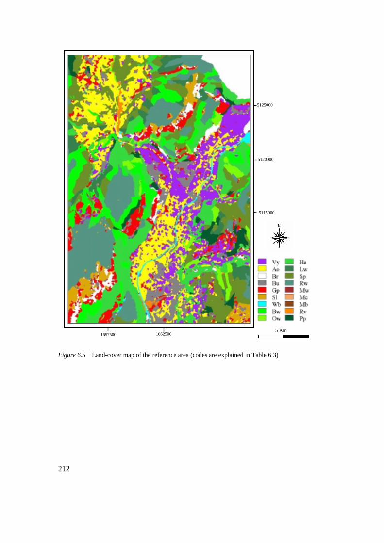
212

Figure 6.5 Land-cover map of the reference area (codes are explained in Table 6.3)

1662500

5125000

5 Km

5120000

5115000

1657500

213

Figure 6.8 Land-cover map of the study area (codes are explained in Table 6.3)

1662500

5125000

5 Km

5120000

5115000

1657500

214

Figure6.9 Map of the natural ecosystems occurring within the study area

1662500

5125000

5 Km

5120000

5115000

1657500

215

Figure 7.1 The space-occupation buffer of the six alternatives displayed on top of the ecosystem map (see legend in Figure 7.2)

Alt.1 Alt.2 Alt.3

Alt.4 Alt.5 Alt.6

Noce R.

Avisio R.

La Rocchetta

Non Valley

La Rupe

Noce R.

Avisio R.

La Rocchetta

Non Valley

La Rupe

Noce R.

Avisio R.

La Rocchetta

Non Valley

La Rupe

Noce R.

Avisio R.

La Rocchetta

Non Valley

La Rupe

Noce R.

Avisio R.

La Rocchetta

Non Valley

La Rupe

Noce R.

Avisio R.

La Rocchetta

Non Valley

La Rupe

216

Figure 7.2 Comparison between the pre-project ecosystem map (Alt.0) and the six scenario maps for a subset of the study area

Alt.0

Legend

Alt.1 Alt.2 Alt.3

Alt.4 Alt.5 Alt.6

217

Figure7.4 The potential-vegetation map (after Pedrotti 1981, 1982)

218

Figure 7.10 Ecosystem-viability map of Alternative 0. The legend refers to the viability value of the ecosystem patches

Figure 7.11 Ecosystem-viability map of Alternative 6. The legend refers to the viability value of the ecosystem patches

219

Figure7.12 Fragmentation-impact maps of the six alternatives (outlined in black). The values indicate the reduction in viability of the affected ecosystems

Alt.1 Alt.2

Alt.3 Alt.4

Alt.5 Alt.6

ecological evaluation for environmental impact … · 3.2.1 what objective of ecological...

Documents