eece 460 : control system design - pid control · eece 460 : control system design pid control guy...
TRANSCRIPT
EECE 460 : Control System DesignPID Control
Guy A. Dumont
UBC EECE
January 2012
Guy A. Dumont (UBC EECE) EECE 460 PID Control January 2012 1 / 32
Contents
1 Background
2 PID StructureThe Textbook PIDAlternate RepresentationsThe Proportional ActionThe Integral ActionThe Derivative ActionSetpoint Weighting
3 Integrator WindupThe ProblemAnti-Windup
4 Uses of PID
Guy A. Dumont (UBC EECE) EECE 460 PID Control January 2012 2 / 32
Background
The Ubiquitous Controller
Almost universally used in industrial control.
PID has proven to be robust and extremely beneficial in the control ofmany important applications.PID stands for:
P: ProportionalI: IntegralD: Derivative
This presentation contains several figures from this excellent book:
K. Åström and T. Hägglund. Advanced PID Control. ISA 2006
Guy A. Dumont (UBC EECE) EECE 460 PID Control January 2012 3 / 32
Background
Historical Note
Early feedback control devices implicitly or explicitly used the ideas ofproportional, integral and derivative action in their structures.
However, it was probably not until Minorsky’s work on ship steeringpublished in 19221, that rigorous theoretical consideration was given toPID control.
This was the first mathematical treatment of the type of controller that isnow used to control almost all industrial processes.
1Minorsky (1922) ’Directional stability of automatically steered bodies’, J. Am.Soc. Naval Eng., 34, p.284
Guy A. Dumont (UBC EECE) EECE 460 PID Control January 2012 4 / 32
Background
Current Situation
Despite the abundance of sophisticated tools, including advancedcontrollers, the Proportional, Integral, Derivative (PID controller) is stillthe most widely used in modern industry
Based on a survey of over eleven thousand controllers in the refining,chemi-cals and pulp and paper industries, 97% of regulatory controllersutilize PID feedback!Many tuning methods
Empirical methods: Ziegler-Nichols, Cohen-Coon. Although used byindustrial practitioners, not recommended, presented for historicalpurposesModel-based methods: Dahlin algorithm, pole-placement, Q-design.Recommended, will be studied in details.
Guy A. Dumont (UBC EECE) EECE 460 PID Control January 2012 5 / 32
PID Structure The Textbook PID
PID Structure
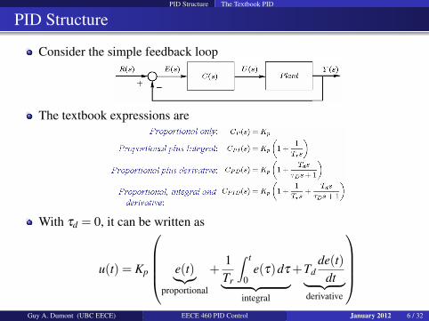
Consider the simple feedback loop
The textbook expressions are
With τd = 0, it can be written as
u(t) = Kp
e(t)︸︷︷︸proportional
+1Tr
∫ t
0e(τ)dτ︸ ︷︷ ︸
integral
+Tdde(t)
dt︸ ︷︷ ︸derivative
where u is the control action and e = ysp− y is the control error.Guy A. Dumont (UBC EECE) EECE 460 PID Control January 2012 6 / 32
PID Structure Alternate Representations
Alternate Representations
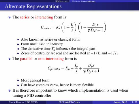
The series or interacting form is
Cseries = Ks
(1+
Is
s
)(1+
DssγsDss+1
)Also known as series or classical formForm most used in industryThe derivative time T ′d influence the integral partZeros of controller are real and are located at −1/Ti and −1/Td
The parallel or non-interacting form is
Cparallel = Kp +Ip
s+
DpsγpDps+1
Most general formCan have complex zeros, hence is more flexible
It is therefore important to know which implementation is used whentuning a PID controller
Guy A. Dumont (UBC EECE) EECE 460 PID Control January 2012 7 / 32
PID Structure Alternate Representations
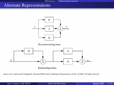
Alternate Representations
Source: K.J. Astrom and T. Hagglund, Advanced PID Control. Published with permission of ISA. c©2009. All rights reserved.
Guy A. Dumont (UBC EECE) EECE 460 PID Control January 2012 8 / 32
PID Structure The Proportional Action
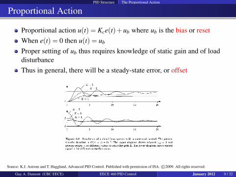
Proportional Action
Proportional action u(t) = Kce(t)+ub where ub is the bias or resetWhen e(t) = 0 then u(t) = ub
Proper setting of ub thus requires knowledge of static gain and of loaddisturbanceThus in general, there will be a steady-state error, or offset
Source: K.J. Astrom and T. Hagglund, Advanced PID Control. Published with permission of ISA. c©2009. All rights reserved.
Guy A. Dumont (UBC EECE) EECE 460 PID Control January 2012 9 / 32
PID Structure The Integral Action
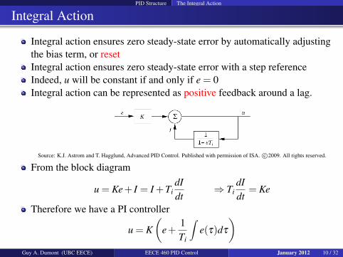
Integral Action
Integral action ensures zero steady-state error by automatically adjustingthe bias term, or resetIntegral action ensures zero steady-state error with a step referenceIndeed, u will be constant if and only if e = 0Integral action can be represented as positive feedback around a lag.
Source: K.J. Astrom and T. Hagglund, Advanced PID Control. Published with permission of ISA. c©2009. All rights reserved.
From the block diagram
u = Ke+ I = I +TidIdt
⇒ TidIdt
= Ke
Therefore we have a PI controller
u = K(
e+1Ti
∫e(τ)dτ
)Guy A. Dumont (UBC EECE) EECE 460 PID Control January 2012 10 / 32
PID Structure The Integral Action
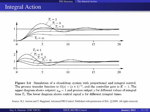
Integral Action
Source: K.J. Astrom and T. Hagglund, Advanced PID Control. Published with permission of ISA. c©2009. All rights reserved.
Guy A. Dumont (UBC EECE) EECE 460 PID Control January 2012 11 / 32
PID Structure The Derivative Action
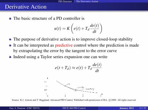
Derivative Action
The basic structure of a PD controller is
u(t) = K(
e(t)+Tdde(t)
dt
)The purpose of derivative action is to improve closed-loop stabilityIt can be interpreted as predictive control where the prediction is madeby extrapolating the error by the tangent to the error curveIndeed using a Taylor series expansion one can write
e(t+Td)≈ e(t)+Tdde(t)
dt
Source: K.J. Astrom and T. Hagglund, Advanced PID Control. Published with permission of ISA. c©2009. All rights reserved.
Guy A. Dumont (UBC EECE) EECE 460 PID Control January 2012 12 / 32
PID Structure The Derivative Action
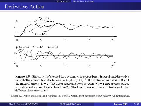
Derivative Action
Source: K.J. Astrom and T. Hagglund, Advanced PID Control. Published with permission of ISA. c©2009. All rights reserved.
Guy A. Dumont (UBC EECE) EECE 460 PID Control January 2012 13 / 32
PID Structure The Derivative Action
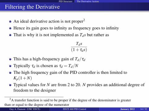
Filtering the Derivative
An ideal derivative action is not proper2
Hence its gain goes to infinity as frequency goes to infinity
That is why it is not implemented as Tds but rather as
Tds(1+ τds)
This has a high-frequency gain of Td/τd
Typically τd is chosen as τd = Td/N
The high frequency gain of the PID controller is then limited toKp(1+N)
Typical values for N are from 2 to 20. N provides an additional degree offreedom to the designer
2A transfer function is said to be proper if the degree of the denominator is greaterthan or equal to the degree of the numerator
Guy A. Dumont (UBC EECE) EECE 460 PID Control January 2012 14 / 32
PID Structure Setpoint Weighting
Setpoint Weighting
A more flexible structure treats the plant output and the setpointseparately
u(t) = Kp
(ep +
1Ti
∫ t
0e(τ)dτ +Td
ded
dt
)where
ep = bysp− y 0≤ b≤ 1
ed = cysp− y 0≤ c≤ 1
The response to load disturbances and measurement noise is unaffectedby b and cThe response to setpoint changes will be affected by the setpoint weightsb and cDecreasing b toward zero reduces the overshoot on setpoint changesThe weight c is usually set to zero to avoid the large derivative action onsetpoint changes (the exception is when the controller is the secondarycontroller in a cascade configuration, as in that case the setpoint rarelychanges in a step manner)
Guy A. Dumont (UBC EECE) EECE 460 PID Control January 2012 15 / 32
PID Structure Setpoint Weighting
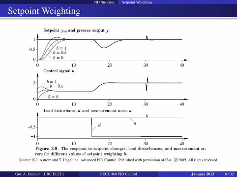
Setpoint Weighting
Source: K.J. Astrom and T. Hagglund, Advanced PID Control. Published with permission of ISA. c©2009. All rights reserved.
Guy A. Dumont (UBC EECE) EECE 460 PID Control January 2012 16 / 32
PID Structure Setpoint Weighting
Setpoint Weighting
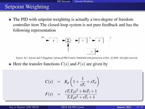
The PID with setpoint weighting is actually a two-degree of freedomcontroller item The closed-loop system is not pure feedback and has thefollowing representation
Source: K.J. Astrom and T. Hagglund, Advanced PID Control. Published with permission of ISA. c©2009. All rights reserved.
Here the transfer functions C(s) and F(s) are given by
C(s) = Kp
(1+
1sTi
+ sTd
)F(s) =
cTiTds2 +bsTi +1TiTds2 + sTi +1
Guy A. Dumont (UBC EECE) EECE 460 PID Control January 2012 17 / 32
Integrator Windup The Problem
Integrator Windup
The ProblemIf the actuator saturates , the system runs in open loopThe integral term may become very largeThe error needs to be of opposite sign for a very long time for integralterm to normal valuesThis might lead to large oscillations
Guy A. Dumont (UBC EECE) EECE 460 PID Control January 2012 18 / 32
Integrator Windup The Problem
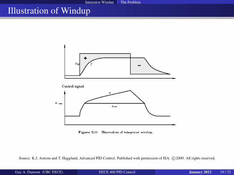
Illustration of Windup
Source: K.J. Astrom and T. Hagglund, Advanced PID Control. Published with permission of ISA. c©2009. All rights reserved.
Guy A. Dumont (UBC EECE) EECE 460 PID Control January 2012 19 / 32
Integrator Windup The Problem
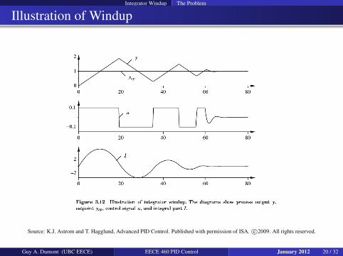
Illustration of Windup
Source: K.J. Astrom and T. Hagglund, Advanced PID Control. Published with permission of ISA. c©2009. All rights reserved.
Guy A. Dumont (UBC EECE) EECE 460 PID Control January 2012 20 / 32
Integrator Windup Anti-Windup
Anti-Windup Schemes
Anti-Windup SchemesBack-calculation and trackingConditional integrationIncremental controller
Guy A. Dumont (UBC EECE) EECE 460 PID Control January 2012 21 / 32
Integrator Windup Anti-Windup
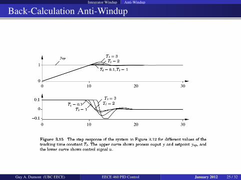
Back-Calculation Anti-Windup
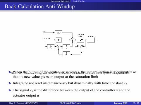
Source: K.J. Astrom and T. Hagglund, Advanced PID Control. Published with permission of ISA. c©2009. All rights reserved.When the output of the controller saturates, the integral action is recomputed sothat its new value gives an output at the saturation limit
Integrator not reset instantaneously but dynamically with time constant Tt
The signal es is the difference between the output of the controller v and theactuator output u
Guy A. Dumont (UBC EECE) EECE 460 PID Control January 2012 22 / 32
Integrator Windup Anti-Windup
Back-Calculation Anti-Windup
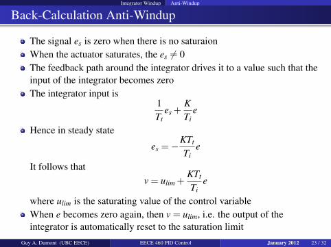
The signal es is zero when there is no saturaionWhen the actuator saturates, the es 6= 0The feedback path around the integrator drives it to a value such that theinput of the integrator becomes zeroThe integrator input is
1Tt
es +KTi
e
Hence in steady state
es =−KTt
Tie
It follows thatv = ulim +
KTt
Tie
where ulim is the saturating value of the control variableWhen e becomes zero again, then v = ulim, i.e. the output of theintegrator is automatically reset to the saturation limit
Guy A. Dumont (UBC EECE) EECE 460 PID Control January 2012 23 / 32
Integrator Windup Anti-Windup
Back-Calculation Anti-Windup
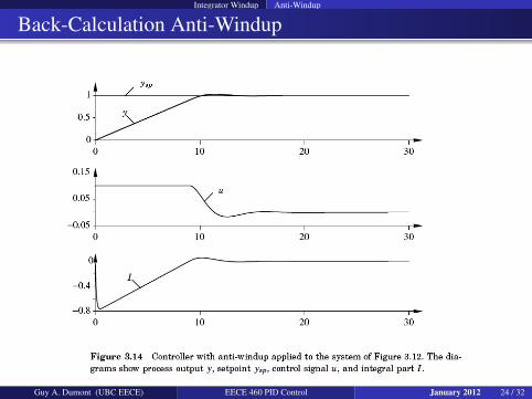
Source: K.J. Astrom and T. Hagglund, Advanced PID Control. Published with permission of ISA. c©2009. All rights reserved.
Guy A. Dumont (UBC EECE) EECE 460 PID Control January 2012 24 / 32
Integrator Windup Anti-Windup
Back-Calculation Anti-Windup
Source: K.J. Astrom and T. Hagglund, Advanced PID Control. Published with permission of ISA. c©2009. All rights reserved.
Guy A. Dumont (UBC EECE) EECE 460 PID Control January 2012 25 / 32
Uses of PID
When To Use PID Control?
Most industrial processes can be controlled by PID controllers as long asperformance requirements are not too stringentApplications of PI Control
Used much more often than PIDFirst-order dynamicsWell damped higher-order dynamics with control only in low bandwidth
Applications of PID ControlSecond-order dynamicsStiff systemsImproves damping, allows higher proportional gain
Guy A. Dumont (UBC EECE) EECE 460 PID Control January 2012 26 / 32
Uses of PID
When Not To Use PID Control?
High-order processes
Systems with long dead time3
Systems with oscillatory modes (for systems with only one oscillatorymode, the non-interacting PID controller may be used)
Important quality control loops call for controllers designed with respectto the disturbance characteristics, rarely giving PID control
3there is some disagreement about this in the process control community, more onthis later
Guy A. Dumont (UBC EECE) EECE 460 PID Control January 2012 27 / 32
Uses of PID
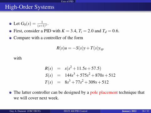
High-Order Systems
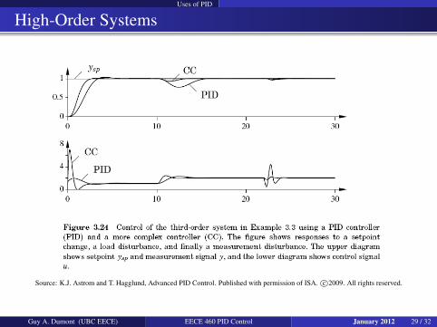
Let G0(s) = 1(s+1)3 .
First, consider a PID with K = 3.4, Ti = 2.0 and Td = 0.6.
Compare with a controller of the form
R(s)u =−S(s)y+T(s)ysp
with
R(s) = s(s2 +11.5s+57.5)
S(s) = 144s3 +575s2 +870s+512
T(s) = 8s3 +77s2 +309s+512
The latter controller can be designed by a pole placement technique thatwe will cover next week.
Guy A. Dumont (UBC EECE) EECE 460 PID Control January 2012 28 / 32
Uses of PID
High-Order Systems
Source: K.J. Astrom and T. Hagglund, Advanced PID Control. Published with permission of ISA. c©2009. All rights reserved.
Guy A. Dumont (UBC EECE) EECE 460 PID Control January 2012 29 / 32
Uses of PID
Systems with Long Time Delays
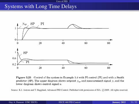
Consider the system
G0(s) =1
1+2se−4s
First, consider a PID controller with K = 0.2 and Ti = 2.5
Compare with a Smith predictor which we will learn to design as aspecial case of pole placement
Guy A. Dumont (UBC EECE) EECE 460 PID Control January 2012 30 / 32
Uses of PID
Systems with Long Time Delays
Source: K.J. Astrom and T. Hagglund, Advanced PID Control. Published with permission of ISA. c©2009. All rights reserved.
Guy A. Dumont (UBC EECE) EECE 460 PID Control January 2012 31 / 32
Uses of PID
Summary
Basics of the PID
Structure and implementation
Windup and remedies
Uses of PID
Next Lecture:PID Design and Tuning
Guy A. Dumont (UBC EECE) EECE 460 PID Control January 2012 32 / 32