t

Entrainment and Optical Properties of an Elevated Forest Fire Plume Transported

into the Planetary Boundary Layer near Washington, D.C.

P. R. Colarco, Goddard Earth Science and Technology Center, University of Maryland-

Baltimore County, NASA Goddard Space Flight Center, Code 91 6, Greenbelt, MD

2077 1

M. R. Schoeberl, NASA Goddard Space Flight Center, Code 916, Greenbelt, MD 20771

B. G. Doddridge, Department of Meteorology, University of Maryland, College Park,

MD 20742 t

L. T. Marufu, Department of Meteorology, University of Maryland, College Park, MD

20742

0. Torres, Joint Center for Earth Systems Technology, University of Maryland-Baltimore

County, NASA Goddard Space Flight Center, Code 916, Greenbelt, MD 20771

E. J. Welton, NASA Goddard Space Flight Center, Code 9 12, Greenbelt, MD 2077 1

Abstract

Smoke and pollutants from Canadian forest fires were transported over the northeastern

United States in July 2002. Lidar observations at the NASA Goddard Space Flight

Center show the smoke fro'm these fires arriving in an elevated plume that was

subsequently transported to the surface. Trajectory and three-dimensional model

calculations confirm the origin of the smoke and show that it mixed to the surface after it

was intercepted by the turbulent planetary boundary layer. Modeled smoke optical

properties agreed well with aircraft and remote sensing observations provided

1

https://ntrs.nasa.gov/search.jsp?R=20030105587 2018-06-27T01:41:45+00:00Z

coagulation of smoke particles was accounted for in the model. Our results have

important implications for the long-range transport of pollutants and their subsequent

entrainment to the surface, as well as the evolving optical properties of smoke from

boreal forest fires.

t

2

Introduction

Ozone (0,) and aerosols transported over long distances can affect air quality at local

and regional scales. For example, the air over the Mediterranean contains a complicated

mix of pollutants transported from Asia, North America, and Europe (1). Saharan dust

transported to the U.S. in the summertime occasionally contributes enough dust to put

portions of Florida out of compliance with U.S. Environmental Protection Agency (EPA)

standards for fine particulate matter (2). High surface-level concentrations of carbon

monoxide (CO) observed during summer 1995 in the eastern and southeastern U.S. were

attributed to pollutants produced and transported in the plumes from large Canadian

forest fires (3). CO and nitrogen oxide (NO, also produced in the forest fires) are

important precursors to the photochemical production of tropospheric ozone. Pollutants

from Canadian and other northern forest fires are frequently transported long distances at

low altitudes behind advancing cold fronts. In this paper, however, we discuss a case in

which smoke from a Canadian forest fire was observed at the NASA Goddard Space

Flight Center (GSFC, 39.02' N, 76.86' W, near Washington, D.C.) in an elevated plume t

that was subsequently mixed to the surface when it was intercepted by the turbulent

planetary boundary layer (PBL).

Over the period July 5 - 9,2002, lightning initiated multiple fires in central Quebec

which burned about 250,000 ha (1 ha = lo4 m2) of boreal forest (4). An upper level low-

pressure system over the Canadian Maritime Provinces coupled with a high pressure

ridge to the west channeled the smoke and pollutants from the fires about 1000 km

southward to the eastern U.S. These plumes were clearly visible in satellite imagery

(Figure Sl), and aerosol optical thickness (AOT) retrievals from the Earth-Probe Total

Ozone Mapping Spectrometer (EP-TOMS) satellite instrument (5) showed that the

plumes were optically thick (Figure 1). During the passage of the plumes the U.S. East

Coast experienced some of the worst air quality days of the summer.

Evolution of Plume Vertical Structure

The NASA Micro-Pulse Lidar NETwork (MPLNET) operates a lidar at GSFC, co-

located with a sudsky photometer in the Aerosol Robotic NETwork (AERONET) (6,7).

Figure 2a shows the MPLNET normalized relative backscatter ratio (8) measured by the t

lidar from July 6 - 9,2002. These measurements show a smoke layer between 2 - 3 km

arriving on July 6. On July 7 the smoke plume rapidly mixed to the surface after about

12:OO UTC. Because the MPLNET signal is completely attenuated above the lowest part

of the smoke plume we do not have any information on the thickness of the smoke layer

on July 7. On July 8 there is still an elevated plume around 2 km. Also shown in Figure

2 is the PBL height at GSFC from the NCAR Model for Atmospheric Transport and

Chemistry (MATCH) (9). The peak height of the MATCH PBL is as high as the top of

the MPLNET signal at 18:OO UTC on July 7, and the subsequent collapse of the model’s

PBL later in the day is coiqcident with the observed plume descent and mixing to the

surface.

Trajectory analyses carried out with the NASA Goddard trajectory model (10) using

the NCEP/NCAR reanalyses (1 1) show that the July 6 - 8 plume observed by MPLNET

over GSFC originated 24 - 48 hours earlier over the Quebec fire regions (Figure S2).

4

Figure 3 shows two-day back-trajectories initialized at GSFC at the altitude of the

MPLNET observed peak bFckscatter in the smoke plume. Trajectories were run for

every hour between 18:OO UTC July 6 (when the smoke arrives) and 12:OO UTC July 8

(when the MPLNET lidar was shut off). We determine the plume altitude by considering

only backscatter altitudes above 0.75 km so that we are not biased by low altitude

anthropogenic pollutants. The times the fires were actively burning in Quebec were

determined from GOES-8 geostationary satellite imagery (12,13) and are indicated by the

grey bars in Figure 3. For each trajectory we show the time and the altitude it crosses

southward of 5 1 O N, roughly the southern edge of the fire region identified from the

GOES-8 imagery. For almost all of the trajectories this point occurred during or shortly

after the period when the fires were active on July 5. The trajectories were between 2 - 6

km altitude over the fire rekion and descended during transport. Trajectories at higher

altitudes over the fire region were transported to GSFC more rapidly than those that were

at lower altitudes.

On July 6 and 7 the surface ozone levels (14) were low over most of the northeastern

U.S. (Figure S3). The pollutants from the fires had not yet been transported to the

surface. Figure 4a shows that on July 8, however, there were very high surface mixing

ratios of ozone (mixing ratio > 125 ppbv) near Washington, D.C., across New Jersey, and

in Ohio and western Pennsylvania. The high surface ozone near GSFC on July 8

occurred shortly after MPLNET observations showed the pollutants from the plume

mixing to the surface. 1

Modeled Smoke Plume

Based on these data and our trajectory calculations we hypothesize that the pollutants

from the fires were transported from Canada toward GSFC in an elevated but subsiding

plume, and that this plume was rapidly mixed to the surface over GSFC on July 7 as it

was intercepted by the turbulent PBL. To test this hypothesis we simulated the evolution

of the smoke plume with a three-dimensional aerosol microphysical and transport model

(15). The model dynamics are from the NCEP/NCAR reanalyses, with parameterizations

for moist convection, precipitation, and boundary layer mixing from MATCH (16,17).

t

Fire locations and timing were prescribed in the model using fire hot spots identified

from GOES-8 imagery. The satellite imagery showed the fires had a distinct diurnal

cycle (Figure 3). In these simulations we treat the smoke aerosol particle size distribution

in 16 discrete size bins space between 0.01 - 1 pm radius. Because the aerosol particles

are all sub-micron in size they are not strongly affected by sedimentation. Particles are

removed by precipitation scavenging or by dry deposition. We determined that neither

of these processes were especially important to our simulated smoke distributions over

GSFC. t

The modeled vertical distribution of smoke at GSFC is sensitive to the height at

which we assume emissions from the fires occur. Global scale models typically inject

biomass burning emissions near the surface or in the PBL (1 8), but there is ample

evidence that intense fires or fires occurring near convective cells can loft smoke and

pollutants to much higher altitudes (19). Starting from the trajectory analysis and data

discussed earlier, in our baseline simulation we add smoke to the model during the active

fire times by distributing it uniformly between 2 - 6 km altitude over the fire hot spots.

Figure 2b shows the resulting vertical smoke mass distribution from the model over

GSFC. The model vertical profile is similar to the MPLNET backscatter observations.

Because the MPLNET observations are attenuated above 2 km on July 7 we cannot use

them to verify the existence of the higher altitude model plume that appears at 4 km late

on July 7. Sensitivity tests show that this plume is from the fires burning on July 6,

whereas the rest of the profile-including the elevated plume on July 8-can be

explained almost entirely by the fires burning on July 5 (consistent with our trajectory

analysis). The smoke plunles were continuously and clearly visible in GOES-8 daytime

imagery. This imagery suggested that most of the smoke over GSFC during this period is

from the fires on July 5 , so it is unlikely the high altitude plume in the model on July 7 is

real.

In order to understand the observed vertical profile at GSFC we considered several

model sensitivity tests. In one case we injected all of the smoke at the surface. Because

of moist convection over the fire regions on July 5 , a large fraction of this smoke was

lifted to 2 - 8 km. In this simulation the vertical profile over GSFC was similar to the

baseline case because both simulations had a great deal of smoke in the 2 - 6 km range.

Because the moist convection was not as strong on July 6 the smoke injected remains

near the surface and the model did not produce a high altitude plume over GSFC on July t

7. The convective mixing parameterization in the model does not greatly redistribute

material already above the surface and below the convective cloud top, so in our baseline

simulation the plume over the fire region remained relatively intact. Likewise, in another

7

sensitivity test where the smoke was injected between 0.5 - 3 km altitude it descended to

the surface rapidly because of subsidence and the vertical profile at GSFC did not agree

well with the MPLNET observations. In summary, the modeled vertical profile was *

similar to the MPLNET observations only when some of the smoke was lifted to 2 - 6

km over the fire regions on July 5. Moist convection over the fires provides a plausible

mechanism for elevating the smoke.

The above discussion largely explains the arrival of an elevated but subsiding plume

at GSFC. Subsidence, however, is not sufficient to explain how the material gets to the

surface at GSFC. We test the importance of PBL entrainment in the model by turning off

the PBL mixing mechanism downwind of the fire regions. For this model run the vertical

profile over GSFC looks similar to our baseline simulation shown in Figure 2b except

that almost all of the aerosvl remains above 500 m (Figure S4). For the baseline

simulation with PBL entrainment, the peak surface mass concentration over GSFC is 140

pg m-3. When PBL entrainment is turned off the peak in the surface mass concentration

at GSFC falls to 4 pg m-3. Figure 4 shows the modeled surface mass concentration of the

smoke aerosol over the northeastern U.S. for the simulations both with and without

entrainment into the PBL. For the case with PBL entrainment the distribution of high

surface mass loadings of aerosol is similar to the distribution of high ozone occurrences

in the EPA data over Ohio, Pennsylvania, and New Jersey on July 8. With PBL

entrainment turned off, however, this correlation is not apparent. We conclude then that

aerosol from the fires was transported mainly in an elevated plume, and that entrainment

into the PBL was critical td bringing the aerosol to the surface near GSFC. Other

8

pollutants transported with the aerosol in the plume (e.g., CO, NO, 0,) would have been

transported in a similar fashion.

July 8 Aircraft Profiles of Plume

The remnant smoke plume observed on July 8 by MPLNET at GSFC was profiled

several times with the University Research Foundation- Advanced Development

Laboratory’s twin engine Piper Aztec-F PA-23-250 research aircraft. The Aztec was

outfitted with an atmospheric research package run by the University of Maryland (20).

Particle scattering measurements were made with a three-channel integrating

nephelometer operating at 450,550, and 700 nm. Aerosol absorption was measured with

a particlehoot absorption photometer operating at 565 nm. Additional measurements

made include particle number concentrations and CO and 0, mixing ratios. Five vertical

profiles were made from near the surface to the aircraft’s operational ceiling at 3 km, four

of which were dominantly influenced by plume material from the Canadian fires. A fifth

profile was flown to the west of the main smoke plume and was more strongly influenced

by anthropogenic pollutants in the PBL. The profiles spanned a region about 200 km

east-west and occurred over a period of about 8 hours. There is some variability in the

smoke aerosol properties owing to the time and space variations in the plume. For the

four profiles which showed evidence of the smoke plume, it was always at about 2 - 3

km altitude and had distinctly different scattering and absorption properties from the

aerosols in the PBL. Back trajectories calculated from this 2 - 3 km range show that for

each profile the air passed over the fire regions during the burning on July 5 at about 4

*

9

km. Finally, for all of these profiles the enhanced aerosol scattering and absorption were

well correlated with enhanced particle number concentrations and CO and 0, mixing

ratios.

Figure 5 shows the narrow layer of aerosol scattering and absorption observed in the

smoke plume on the Aztec profile flown above Easton, MD (38.80' N, 76.06' W, about

70 km E of GSFC, profile flown between 19:45 - 20:12 UTC). Also shown are the

scattering and absorption profiles from the MPLNET data at GSFC at 11:35 UTC July 8

(determined from the retrieved extinction profile and the AERONET single scatter albedo

in Table l), which show a peak in the 2 - 3 km altitude range. The MPLNET data also

show a strong scattering and absorption peak below 1 km. Because of the high

extinction-to-backscatter ratio determined for the MPLNET lidar profile it is likely that

this low altitude peak is due to remnants from the smoke plume intercepted at the surface

on July 7. Figure 5 also shows the modeled scattering and absorption profiles at GSFC at

20:OO UTC on July 8. The model clearly shows an elevated smoke layer, although it is at

a lower altitude (1.5 - 2.5 km) than the Aztec or MPLNET profiles. The peak magnitude

of the modeled scattering and absorption are smaller than the lidar or aircraft

measurements, but the vertical extent of the smoke is much greater in the model than in

the observations. The model vertical grid spacing varies from 100 - 200 m below 1 km

altitude, and increases to about 500 m at 2 km and 800 m at 5 km. The vertical grid

spacing is thus too coarse to adequately resolve the sharp peaks seen with the aircraft and

lidar.

10

Smoke Plume Optical Properties

Our understanding of smoke optical properties has increased in recent years thanks to

field campaigns such as the Smoke, Clouds, and Radiation-Brazil (SCAR-B) experiment

(21). While most such experiments have focused on smoke from tropical fires, there

t

have been relatively few experiments devoted to smoke from boreal forest fires. The

spectral AOT from measurements the Aztec, AERONET, and EP-TOMS observations

thus contribute important constraints on optical properties of boreal forest fire smoke that

has been transported over long-distances. The AERONET AOT measurements at GSFC

on July 7 - 8 were among the highest values ever recorded in the entire network (22).

Additionally, the Angstrom exponents derived from the AERONET and Aztec

measurements near GSFC are quite low compared to observations made closer to boreal

forest fire sources (23). These observations are consistent with a smoke plume in which

the particles have grown ("aged") considerably during transport. Various mechanisms

can explain the smoke particle growth during transport, including hygroscopic water

uptake (24), condensation of volatile organic species (25), and coagulation (26,27).

Integrating these aging mechanisms and the observations into our aerosol model is a

formidable challenge. We focus here on the importance of coagulation in modifying the

aerosol particle size distribution by running simulations with and without this process.

For both simulations we initialize the model with a particle size distribution

representative of fresh boreal smoke emissions and make no assumptions about the

smoke composition other than its refractive index (see supplemental online material).

Without coagulation, the particle size distribution is modified only slightly by removal 1

1 1

processes. With coagulation the particle size distribution shifts to larger particles as

expected (Figure SS).

Table 1 summarizes the observed and modeled optical properties of the smoke plume

near GSFC on July 8. The EP-TOMS 380 nm AOT is from the closest satellite footprint

to GSFC, and is 20 - 30% larger than the AERONET measurements occurring within 30

minutes of the satellite overpass. This difference is likely related to the large EP-TOMS

footprint relative to the essentially point-like AERONET measurement, and is possibly t

affected by sub-gridscale cloud contamination. The AERONET measurements at longer

wavelengths are comparable to the column AOT measurements from the Aztec profiles

of the smoke plume. The model AOT is at the high end of the range of AERONET and

Aztec measurements shown, but is slightly smaller than the EP-TOMS retrieval.

The single scatter albedo from the AERONET and Aztec measurements indicate a

weakly absorbing aerosol. The model single scatter albedo agrees best with the

AERONET measurements, although the AERONET and Aztec values are almost within

each other’s error bars. The lower single scatter albedo determined from EP-TOMS is

mainly because the optica1,effective radius of the smoke particle size distribution

assumed in the retrieval is too small compared to the AERONET measurements of this

plume. Underestimating the particle effective radius makes the aerosol look more

absorbing than it actually is, but has only a small effect on the retrieved AOT (5). Note

that the model calculated and AERONET retrieved single scatter albedos are relatively

independent of wavelength for the cases discussed here.

Scattering angstrom exponents determined inside the smoke plume from the Aztec

12

* nephelometer measurements (20) are recorded for each wavelength pair in Table 1 . For

the model run with particle coagulation the Angstrom exponents calculated at GSFC on

July 8 are similar to the values determined from the aircraft measurements. Without

coagulation, however, the model's values are much larger than and outside the error bars

of the observations. The comparison is somewhat ambiguous between the model and

AERONET scattering Angstrom exponent for the 440 - 670 nm wavelength pair. An

explanation for this is that the model particle size distribution has too many large

particles compared to the AERONET retrieved particle size distribution (Figure S5). The

comparison of the model size distribution to AERONET is much better when coagulation

is accounted for, however,*as the model substantially underestimates the mean particle

radius when coagulation is ignored.

There are uncertainties in comparing the model to these measurements. Because of

its coarse spatial resolution it is difficult to justify comparing the model at the scale of a

single grid-column to the essentially point-like measurements from the aircraft profiles

and the sunphotometer measurements. On the other hand, the spatial extent of the plume

is comparable to the model grid size. Furthermore the model does not have significant

spatial or temporal variability in the computed optical properties for the grid points

surrounding GSFC. The largest uncertainties are associated with the choice of refractive

index used in the calculations (28). Small variations in the wavelength dependent AOT

calculated can lead to large variations in the Angstrom exponent. This is a primary t

indicator of particle size, however, so that despite whatever uncertainties we may have in

the refractive index there is always a clear difference in the angstrom exponents when

I

the model runs with and wkhout coagulation are compared. The model results are much

more coherent with the observations for the runs with coagulation than they are for runs

which neglect this process. This leads us to conclude that coagulation is important to

modifying the initial aerosol particle size distribution and can explain at least some of the

observed spectral dependence in the AOT far downwind. This has implications to

radiative forcing calculations as well as retrievals of aerosol properties made from

satellite observations. Neglecting the aging of aerosol particles in smoke plumes and

instead relying on particle size distributions measured near the smoke emission point for

these calculations will yield the wrong spectral dependence in the optical properties.

I

Conclusions

Our analysis of the transport of a Canadian forest fire plume over the eastern U.S.

during July 2002 demonstrates that an important mechanism for transporting pollutants

from elevated layers to the surface is by entrainment into the PBI, of a gradually

subsiding plume. An aerosol microphysics and transport model driven by assimilated

meteorology confirms this mechanism. This model also tested various assumptions about

the initial injection altitude of the plume from the fires. The modeled vertical profile at

GSFC was similar to the MPLNET observations provided the majority of the smoke was

initially injected into a 2 - 6 km altitude layer, as suggested by our trajectory

calculations. Moist conveation over the fire regions can explain how this elevated layer L I

developed. Our simulation yielded spectral AOT values similar to those observed with

the aircraft flights and sunphotometer measurements provided we accounted for

14

modification of the smoke particle size distribution by coagulation. The aerosol lifting

and deposition mechanisms discussed here have important implications for the long-

range transport of smoke aerosols from boreal forest fires and their effects at the surface

through subsequent coupling to the PBL downstream. Accounting for the modification

of the smoker aerosol particle size distribution due to coagulation and other modification ‘1

processes is also important for correctly determining the direct radiative effect of the

aerosol, as well as for quantitative retrievals of aerosol properties from remote sensing

measurements (29,30).

I

‘1

‘1

1s

I

t

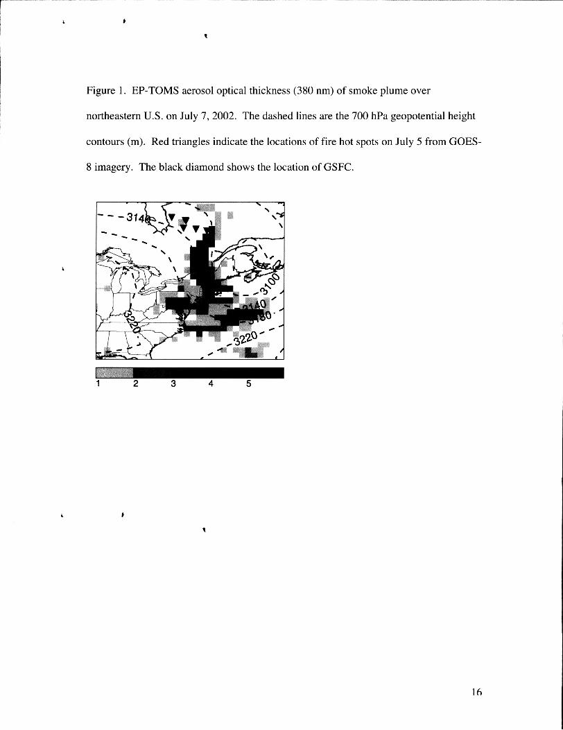
Figure 1. EP-TOMS aerosol optical thickness (380 nm) of smoke plume over

northeastern U.S. on July 7,2002. The dashed lines are the 700 hPa geopotential height

contours (m). Red triangles indicate the locations of fire hot spots on July 5 from GOES-

8 imagery. The black diamond shows the location of GSFC.

t

16

Figure 2. Vertical profile of aerosol at GSFC from (a) MPLNET and (b) the aerosol

model. The white line is the MATCH PBL height. Note that the MPL did not collect

data after about 12:OO UTC on July 8 until late on July 9.

L

8 9 6 7 8 9

- 6 ((I w 5- July 2002 ’ July 2002

6

Normalized Relape Backscatter 1 0 [counts ps pJ km’] 0

B

Model Smoke Mass 150 Concentration [pg mq

17

Figure 3. Two-day back trajectories from GSFC at the altitude of the observed peak

MPLNET backscatter. The color shading of the line indicates the start time of the

trajectory. The grey bars show the times the fires were active in Quebec as inferred from

GOES-8 imagery. The black diamonds on each trajectory show the time at which the

trajectory passed south of 5 1 O N.

8

6

2

0 5 6 7 8 9

July

0207061 8 Start Time 0207081 2

t

18

1 #

Figure 4. (a) EPA peak 1-hour average surface ozone mixing ratios on July 8,2002.

Also shown are the modeled surface mass concentrations of smoke particles for the high-

injection model runs (b) with and (c) without PBL entrainment.

Observed Surface O3 Mixing Ratio [ppbl 60 80 100 110 125 Modd Surface Mass Concenttatlon tug m7 5 10 25 50 100

I

I

a

t

19

Figure 5. Observed and modeled aerosol (a) scattering and (b) absorption profiles at

Easton on July 8, 2002. Shown are the Aztec profiles (diamonds:) and the model profiles

at 20:OO UTC (thick lines). Also shown are the MPLNET measurements of scattering

1 and extinction at GSFC at 11:30 UTC (thin line). t

a) Scattering Coefficient (550 nm] 5 h Easton (Aztec)

0.0000 0.0005 0.0010 0.0015 0.0020 Scattering Coefficient [m-'1

b) Absorption Coefficient [565 nm] 5 6

0 20 40 60 80 100 120 140 Absorption Coefficient [Mm '1

a

1 t

Model (coag.) Model (no coag.)

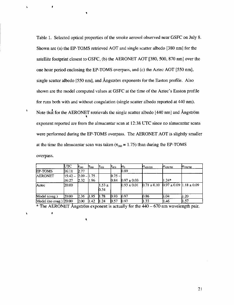
Table 1. Selected optical properties of the smoke aerosol observed near GSFC on July 8.

20:OO 2.36 1.95 1.78 3.93 0.97 3.86 1.04 1.20 20:OO 2.00 1.42 1.24 3.57 3.97 1.33 1.46 1.57

Shown are (a) the EP-TOMS retrieved AOT and single scatter albedo [380 nm] for the

satellite footprint closest to GSFC, (b) the AERONET AOT [380,500, 870 nm] over the

one hour period enclosing the EP-TOMS overpass, and (c) the Aztec AOT [550 nm],

single scatter albedo [550 nm], and Angstrom exponents for the Easton profile. Also

shown are the model computed values at GSFC at the time of the Aztec’s Easton profile

for runs both with and without coagulation (single scatter albedo reported at 440 nm).

1 Note that for the AERONET retrievals the single scatter albedo [440 nm] and Angstrom

exponent reported are from the almucantar scan at 12:38 UTC since no almucantar scans

t

were performed during the EP-TOMS overpass. The AERONET AOT is slightly smaller

at the time the almucantar scan was taken = 1.75) than during the EP-TOMS

overpass.

t

21

References: 1 I

1 J. Lelieveld et al., Science 298,794 (2002). 2 J. M. Prospero, I. Olmez, M. Ames, Water Air Soil Poll. 125,291 (2001). 3 G. Wotawa, M. Trainer, Science 288,324 (2000). 4 http://www.nrcan.gc.ca/cfs-scf/science/prodserv/firerepo~archives/july 1002-e.html 5 0. Torres et al., J. Atmos. Sci. 59,398 (2002). 6 E. J. Welton, J. R. Campbell, J. D. Spinhirne, V. S . Scott, in Proceedings SPIE, Vol. 4153: Lidar Remote Sensing for Industry and Environmental Monitoring, U. N. Singh, T. Itabe, N. Sugimoto, Eds. (SPIE, Bellingham, WA, 2001), pp. 151-158. 7 B. N. Holben et al., Remote Sens. Environ. 66, 1 (1998). 8 J. R. Campbell et al., J. Atm. Ocean. Tech. 19,431 (2002). 9 P. J. Rasch, N. M. Mahowald, B. E. Eaton, J. Geophys. Res. 102,28,127 (1997). 10 D. R. Allen, M. R. Schoeberl, J. R. Herman, J. Geophys. Res., 104,27,461 (1999). 1 1 E. Kalnay et al., B. Am. Meteorol. SOC. 77,437 (1996). 12 E. M. Prins, W. P. Menzel, Znt. J. Rem. Sens. 13,2783 (1992). 1 3 http://rsd.gsfc.nasa.gov/users/marit/projects/canada_smoke/ 14 Data are courtesy of the U.S. Environmental Protection Agency: http://www .epa.gov/airnow/2002. 15 0. BjToon, R. P. Turco, D. Westphal, R. Malone, M. S . Liu, J. Atmos. Sci. 452,123

16 P. R. Colarco, 0. B. Toon, 0. Torres, P. J. Rasch, J. Geophys. Res. 106, art. no. 4289

17 A description of the model is provided in the online supporting material. 18 C. Liousse et al., J. Geophys. Res. 101, 19,411 (1996). 19 M. Fromm et al., Geophys. Res. Let. 27, 1,407 (2000). 20 B. F. Taubman, L. T. Marufu, C. A. Piety, B. G. Doddridge, R. R. Dickerson, J. Geophys. Res. (submitted 2003). 21 Y. J. Kaufman et al., J. Geophys. Res. 103,31783 (1998). 22 T. F. Eck et al., Geophys. Res. Let. (submitted 2003). 23 N. T. O’Neill et al., J. Geophys. Res. 107, 10.1029/2001JDO00877 (2002). 24 P. V. Hobbs, J. S. Reid, R. A. Kotchenruther, R. J. Ferek, R. Weiss, Science 275, 1776 (1997). 25 J. S. Reid et al., J. Geophys. Res. 103,32059 (1998). 26 D. L. Westphal, 0. B. Toon, J. Geophys. Res. 96,22,379 (1991). 27 L. F. Radke, A. S. Hegg, P. V. Hobbs, J. E. Penner, Atmos. Res. 38,3 15 (1995). 28 Uncertainties in the modeled optical properties due to the choice of refractive index are discussed in more detail in the supporting online material. 29 Suppprting online material, www .sciencemag.org, Model Description, Uncertainties in Computed Optical Properties, Figs. S 1, S2, S3, S4, S5, Tables SI, S2. 30 This research was partihy funded by the NASA Interdisciplinary Science program. BGD and LTM acknowledge support from Maryland Department of Environment and

a

( 1 98 8). t

(2002).

1

22

Mid-Atlantic and Northeast Visibility Union. The Micro-Pulse Lidar NETwork (MPLNET) is funded by the NASA Earth Observing System. B. N. Holben provided AERONET data. T. F. Eck and B. F. Taubmann provided valuable comments to this manuscript.

t

Supplemental Online Material

Model Description

Our model (1,2) couples dynamical fields from the NCEP/NCAR reanalyses (3) and

the NCAR Model for Atmospheric Transport and Chemistry (MATCH) (4) to the

University of Colorado/NASA Ames Community Aerosol and Radiation Model for

Atmospheres (CARMA) (5). CARMA is a bin-resolving microphysical model which

solves the aerosol continuity equation for source, transport, removal, and t

transformational processes (e.g., coagulation). The reanalyses and MATCH provide

wind, temperature, and pressure fields, as well as convective mass fluxes, precipitation

rates, and eddy-diffusion coefficients for mixing in the PBL. These fields are archived

globally every six hours at the resolution of the reanalyses (approximately 1.875" x

1.875' in the horizontal and 21 vertical sigma levels from the surface to about 15 km).

CARMA is run on a limited domain encompassing most of North America and the North

Atlantic Ocean with the same grid spacing. The model is run from July 5 to 11 with an

1800 second time step and we linearly interpolate the input dynamical fields to the

current time step. t

The timing and locations of fire hot spots are determined from the 4 ym and 11 ym

GOES-8 channels (6,7). The locations of fire hot spots on July 5,2002, are shown in

Figure 1, and the active fire times are indicated by the grey bars in Figure 3. We assume

that the fires are emitting at a constant rate while the fires are active. We assume a flux

of 5 x kg m-2 s-' per hot spot, which yields total emissions of about 1.5 Tg. The

24

injection altitude of the smQke particles is as described in the text.

We do not have a dataset to quantify the actual smoke emissions. A rough estimate

was obtained by assuming typical land-surface characteristics and assuming 250,000 ha

of land burned (8), where we assume average biofuel loadings of 17 Mg ha-' of above-

ground carbon material (consumed with 26% efficiency) and 108 Mg ha" of ground-level

carbon material (consumed with 6% efficiency) (9). Assuming the carbon content is 45%

of the total dry matter mass and applying a typical emission factor of 0.013 g PM2.5 per

1 g dry matter burned (10) we estimate total PM2.5 emissions from the fires to be about

0.10 Tg, which is about a factor of 10 smaller than the emissions used in the model. The

emissions used in the model were tuned to give reasonable agreement between the model

and observed aerosol optic'al properties at GSFC. Reducing the model emissions to 0.10

Tg results in a dramatic decrease in the AOT at GSFC so that the model greatly

underestimates the observed AOT. We point out that there is considerable uncertainty in

this emission estimate because we are applying average land spatial characteristics and

assuming a smoke emission factor which may not be representative of the actual fires.

Alternatively, because of numerical diffusion and the model's coarse spatial resolution

we may require unrealistically large total emissions in order to get 200 km x 200 km grid

cells to represent aerosol distributions which might be present on much smaller scales.

Higher spatial resolution simulations will answer this question, but for now we are

satisfied to get reasonably AOT agreement between the model and the observations. t

The injected smoke particles are distributed across 16 size bins spaced

logarithmically in radius between 0.01 - 1 pm. There are observations of coarse mode

25

particles with radius > 1 pm in boreal forest fire plumes (1 1). These particles are usually

ash, partially burned foliage, and lofted soil particles that make up a small fraction of the

total particulate mass, have large fall speeds, and are less optically efficient than the fine

mode particles. We neglect these large particles in this study of long-range transport of

smoke, although they may be important to the properties of the smoke plume near the

sources. We assume the smoke particles have a lognormal size distribution with a

volume mode radius of 0.145 pm and a standard deviation of 2.00 (1 2). This initial

particle size distribution is similar to a recent climatology of South American and African

biomass burning aerosols determined from AERONET observations near major source

regions (13). The density of the particles is assumed to be 1.35 g cm-3 (14).

Sedimentation, dry deposition, and precipitation scavenging rates are determined for each

size bin (2). For some of our simulations we allow coagulation to modify the particle

size distribution, which increases the mean radius of the particle size distribution at a rate

approximately proportional to the air temperature, the square of the particle number

concentration, and the invAse of the particle radius (15). Our algorithm (5) preserves the

total aerosol volume but decreases the number concentration of particles as small

particles stick together and grow larger.

t

We calculate the smoke optical properties in the model assuming a wavelength

dependent refractive index based on AERONET almucantar retrievals of the smoke

plume over GSFC (16,17). AERONET inverts aerosol optical properties by fitting

radiance measurements over a wide angular and spectral range (the almucantar scan) to a

pre-computed look-up table of radiances. The retrieval provides the column integrated

26

aerosol particle size distribution, and the complex index of refraction and single scatter

albedo at four reference wavelengths (440,670,870, and 1020 nm). Because of

restrictions on the inversion the retrievals are only valid for almucantar scans taken at

high solar zenith angle (1 45") and high AOT ( T ~ ~ ~ 2 0.4). Additional screening criteria

may further restrict the availability of retrievals (1 8). For this study we use a complex

index of refraction from the AERONET almucantar scan taken at 12:38 UTC at GSFC on

July 8,2002 (Table Sl). Refractive indices at other than the reference wavelengths are

computed by a least-squares second-order polynomial fit to the retrieved values. These

refractive indices are representative of the atmospheric column over GSFC at the time the t

scan was taken, although because of the high AOT of the smoke plume (Table 1) we

expect that contributions from other aerosols present (e.g., anthropogenic pollutants) will

have only a minor effect on the column integrated value.

Uncertainties in Computed Optical Properties

The are uncertainties in the modeled smoke optical properties associated with

temporal and spatial variations in the smoke plume. The model has a relatively coarse

spatial resolution such that a single grid cell is comparable to the entire spatial extent of

the Aztec measurements. The model also has a coarse temporal resolution in the sense

that we have made some simple assumptions about the timing of the smoke emissions.

The net result is that there is not much variability in the modeled particle size distribution

and computed Angstrom exponents at GSFC or in surrounding grid cells over the period

12:OO UTC July 8 - 0O:OO UTC July 9. In contrast, there is significant variability in the

27

Angstrom exponents from the Aztec profiles that sampled the smoke plume.

Additionally, there is variability in the refractive index retrieved from AERONET

depending on which almucantar scan is used and at which site. For example, AERONET

measurements at the Maryland Science Center in Baltimore, MD (39.27" N, 76.62' W),

observed the same smoke plume on July 8 that was seen at GSFC, but because of the

spatial and temporal variability of the plume somewhat different refractive indices were

retrieved. In Table S2 we summarize the Angstrom exponents from the Aztec flights

sampling the smoke plume and from the model for various choices of refractive index.

The model results shown are all from the simulation in which particles were allowed to

coagulate. For most choices of refractive index shown in Table S2 the computed

Angstrom exponents fit somewhere in the range of values observed by the Aztec. The

tendencies are for a decrease in Angstrom exponent with an increase in either the real or

imaginary component of the refractive index. Although we do not show the variability of

t

Angstrom exponents for the model runs without coagulation it is clear that for a given

choice of refractive index the Angstrom exponents will always be larger in the run

without coagulation than in the run with coagulation. For a reasonable range of refractive

index, then, the model looks most like the aircraft measurements when coagulation is

accounted for. This implies that the smoke particles are larger at GSFC than they were

assumed to be at the source region, and that coagulation provides a reasonable

explanation for how this growth occurred.

Additional uncertainties in the modeled aerosol optical properties computed could

also result from other assumptions made about the aerosol microphysics. We have not t

28

considered hygroscopic growth of the smoke aerosols during transport, although since the

Aztec profiles show that the relative humidity at the 2 - 3 km altitude of the smoke plume

was less than 30% this process is probably unimportant to modifying the smoke optical

properties. We also did not consider that the smoke plume may have mixed with clouds

or other aerosol species, although because the plumes were mainly transported in an

elevated layer they were probably largely unaffected by clouds or aerosols until after they t

had been intercepted by the PBL.

29

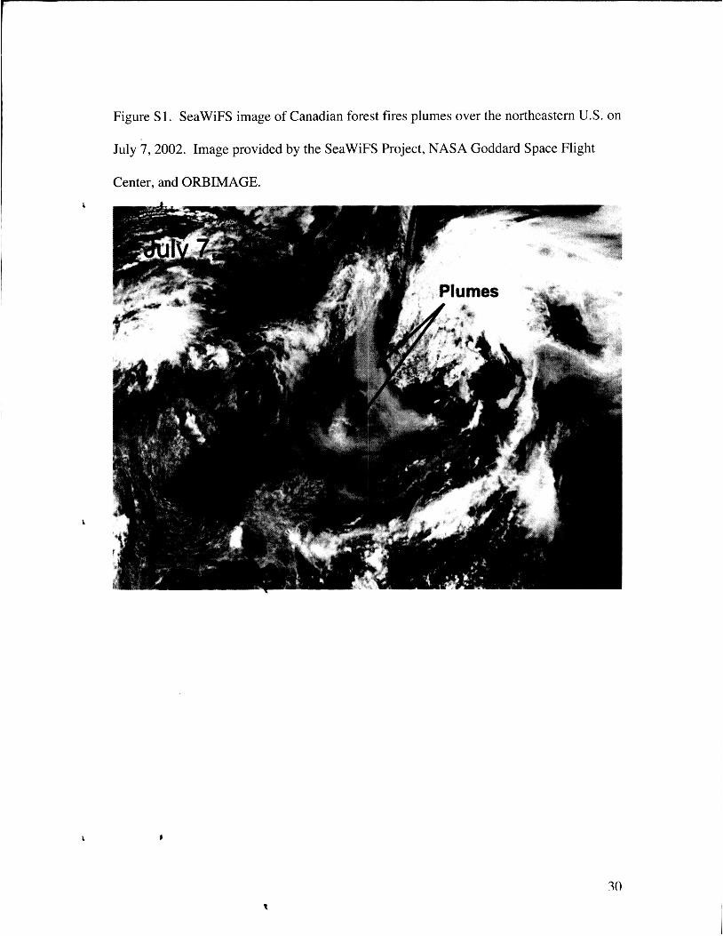
Figure S 1. SeaWiFS image of Canadian forest fires plumes over the northeastern U.S. on

July 7,2002. Image provided by the SeaWiFS Project, NASA Goddard Space Flight

Center, and ORBIMAGE.

L I

Figure S2. Two-day back-trajectories from GSFC. The shading of the trajectories

indicates the initialization time of the trajectory, with initial times and altitudes consistent

with Figure 3. The black diamond shows the location of GSFC. Red triangles are the

GOES-8 fire locations on July 5,2002. The dashed line shows the 5 1" N latitude,

approximately the southern edge of the fire region.

a

0207061 8 Start Time 0207081 2

I

31

Figure S3. EPA peak 1-hour average ozone mixing ratios for July 6 - 9,2002.

7

July 8, 2002’ ( 7 42. \

“y.‘

Surface 0, mixing ratio [ppb]

. &$ July6,2002’

Surface 0, mixing ratio [ppb]

’ ‘.;d July 7,2002‘

60 80 100 110 125 Surface 0, mixing ratio [ppb]

July 9, 2002‘ ,--- ---

60 80 100 110 125 I F, ,

60 80 100 110 125

32

a

a

Figure S4. Observed and modeled aerosol vertical profiles. As in Figure 2 except that

the model shown in (b) is from a run with PBL entrainment turned off.

7 8 9 6 7 8 9

(1 *- * .*1-

July 2002

Concentration [pg md]

July 2002

[counts ps pJ kmq

6

0 Normalized Relative packscatter 1 0 Model Smoke Mass 150

33

a

a

Figure S5. Observed and modeled aerosol particle size distribution at GSFC on July 8,

2002. The size distributions are integrated over the atmospheric column and normalized

to the same peak value in the volume. Recall that the model does not contain

anthropogenic aerosols in the PBL, which are seen by AERONET if present. Red line is

the size distribution from the baseline model run with coagulation turned off. Blue line is

from the baseline model run with coagulation turned on. Black dashed line is the

AERONET retrieval.

0.50 F

t

0.01

Model (No Coagulation) Model (Coagulation)

0.1 0 radius bm]

1 .oo

a

34

Table S 1. Wavelength dependent complex index of refraction from the AERONET

1 h[nml 1 Ne,

440 1.524 - 0.0056i

670 1.554 - 0.0043i t

870 1.573 - 0.0038i

1020 1.583 - 0.0037i

t

t

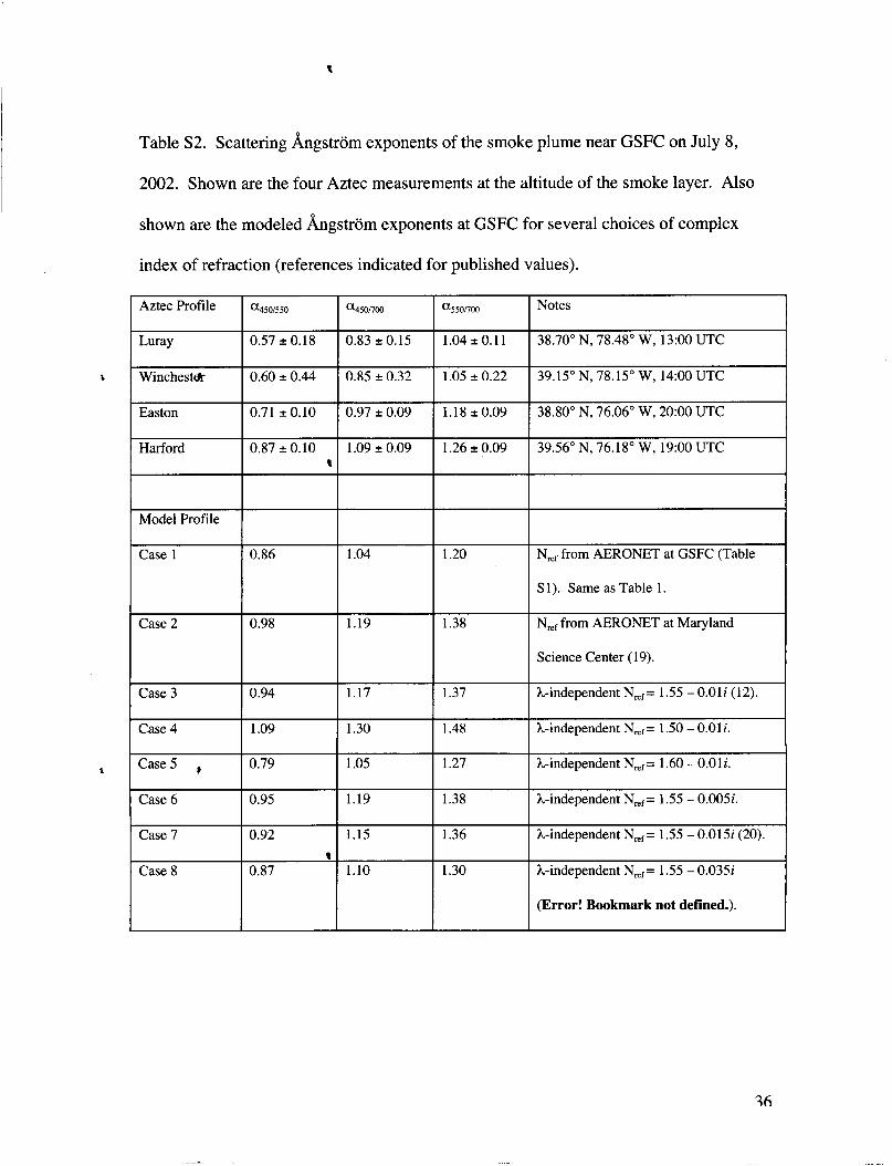
Table S2. Scattering Angstrom exponents of the smoke plume near GSFC on July 8,

2002. Shown are the four Aztec measurements at the altitude of the smoke layer. Also

shown are the modeled Angstrom exponents at GSFC for several choices of complex

index of refraction (references indicated for published values).

Easton

Aztec Profile a4501550 a450/700 a550/700

Luray 0.57 2 0.18 0.83 2 0.15 1.04 2 0.1 1 t Winchest& 0.60 2 0.44 0.85 2 0.32 1.05 2 0.22

0.71 2 0.10 0.97 2 0.09 1.18 2 0.09

Harford 0.87 2 0.10 1.09 0.09 1.26 2 0.09 %

Model Profile

Case 5 , Case 6

Case 7

I I I

Case 4 I 1.09 I 1.30 I 1.48

0.79 1.05 1.27

0.95 1.19 1.38

0.92 1.15 1.36 ; Case 8

Notes

38.70" N, 78.48" W, 13:OO UTC

39.15" N, 78.15" W, 14:OO UTC

38.80" N, 76.06" W, 20:OO UTC

39.56" N, 76.18" W, 19:OO UTC

N,, from AERONET at GSFC (Table

Sl). Same as Table 1.

N,, from AERONET at Maryland

Science Center (1 9).

A-independent Nref= 1.55 -0.Oli (12).

h-independent Nref= 1 S O - 0.01 i.

A-independent N,, = 1.60 - 0.0 1 i.

A-independent Nref= 1.55 - 0.005i.

A-independent Nref= 1.55 -0.015 (20).

A-independent NEf= 1.55 - 0.035

(Error! Bookmark not defined.).

' Referenhes:

1 P. R. Colarco, 0. B. Tooh, 0. Torres, P. J. Rasch, J . Geophys. Res. 106, art. no. 4289 (2002). 2 P. R. Colarco, 0. B. Toon, B. N. Holben, J . Geophys. Res. (in press). 3 E. Kalnay et al., B. Am. Meteorol. SOC. 77,437 (1996). 4 P. J. Rasch, N. M. Mahowald, B. E. Eaton, J . Geophys. Res. 102,28,127 (1997). 5 0. B. Toon, R. P. Turco, D. Westphal, R. Malone, M. S. Liu, J . Atmos. Sci. 45,2,123 (1988). 6 E. M. Prins, W. P. Menzel, Int. J . Rem. Sens. 13,2783 (1992). 7 http://rsd.gsfc.nasa.gov/users/marit/projects/canada_smoke/ 8 http://www .nrcan.gc.ca/cfs-scf /science/prodserv/f iuly 1002-e.html 9 E. S. Kasischke et al., in Biomass Burning and its Inter-relationships with the Climate System, J. L. Innes, Ed. (Kluwer, Dordrecht, 2000). 10 M. 0. Andreae, P. Merlet, Glob. Biogeochem. Cyc. 15,955 (2001). 1 1 L. F. Radke et al., in Global Biomass Burning, J. S. Levine, Ed. (MIT, Cambridge, MA, 1991), chap. 28. 12 D.L. Westphal, O.B. Toon, J . Geophys. Res. 96,22,379 (1991). 13 0. Dubovik et al., J . Atmos. Sci. 59,590 (2002). 14 J. S. Reid, P. V. Hobbs, J . Geophys. Res. 103,32,013 (1998). 15 H. R. Prupacher, J. D. Klett, Microphysics of Clouds and Precipitation (Kluwer,

16 B. N. Holben et al., Remote Sens. Environ. 66, 1 (1998). 17 0. Dubovik, M. D. King, J . Geophys. Res. 105,20,673 (2000). 18 http://aeronet.gsfc.nasa.gov/ 19 T. F. Eck et al., Geophys. Res. Let. (submitted 2003). 20 0. Torres et al., J . Atmos. Sci. 59,398 (2002).

a

Dordrecht, 1997). I

I

37