erd working paper no. 62 - asian development bank · erd working paper no. 62 a small...
TRANSCRIPT


ERD Working Paper No. 62
A Small Macroeconometric Modelof the Philippine Economy
GEOFFREY DUCANES, MARIE ANNE CAGAS, DUO QIN, PILIPINAS QUISING,AND NEDELYN MAGTIBAY-RAMOS
January 2005
Geoffrey Ducanes and Marie Anne Cagas are consultants, Duo Qin is an economist, and Pilipinas Quising and NedelynMagtibay-Ramos are economic analysts in the Economics and Research Department, Asian Development Bank.

Asian Development BankP.O. Box 7890980 ManilaPhilippines
©2005 by Asian Development BankJanuary 2005ISSN 1655-5252
The views expressed in this paperare those of the author(s) and do notnecessarily reflect the views or policiesof the Asian Development Bank.

FOREWORD
The ERD Working Paper Series is a forum for ongoing and recentlycompleted research and policy studies undertaken in the Asian DevelopmentBank or on its behalf. The Series is a quick-disseminating, informal publicationmeant to stimulate discussion and elicit feedback. Papers published under thisSeries could subsequently be revised for publication as articles in professionaljournals or chapters in books.

CONTENTS
Abstract vii
I. INTRODUCTION 1
II. BRIEF OVERVIEW OF THE ECONOMY AND THE DATA 3
III. THE STRUCTURE OF THE MODEL 4
A. Private Consumption Block 4B. Investment Block 4C. Government Block 4D. Trade Block 5E. Production Block 5F. Price Block 6G. Monetary Block 7H. Employment Block 7
IV. SIMULATION EXPERIMENTS 8
A. Model Evaluation 8B. Impact Analysis 12
V. CONCLUSION 18
Appendix: Specification and structure of the model 21References 46

ABSTRACT
This paper describes a small quarterly macroeconometric model of the Philippineeconomy. The model consists of sectors of private consumption, investment,government, trade, production, prices, money, and labor. The equilibrium-correctionform is used for all the behavioral equations. The tracking performance of the model,both within-sample and out-of-sample, is evaluated and found satisfactory. Policysimulations indicate it is crucial that the Philippine government address its debtproblem for it to achieve higher future growth. Oil price simulations also showthe country is highly vulnerable to external shocks.

I. INTRODUCTION
This paper presents a model of the Philippine economy, which was developed as part of the AsianDevelopment Bank’s (ADB) project to develop macroeconometric models of its major debt membercountries. These models are to be used for forecasting and policy simulation.
There are several existing Philippine macroeconometric models.1 The major ones still in use arethe PIDS-NEDA Annual Model, NEDA Quarterly Macroeconomic Model (NEDA QMM), and AteneoMacroeconomic Forecasting Model (AMFM).2 The PIDS-NEDA Annual Model is the oldest of the grouphaving been started in the mid-1980s but later modified into several versions, the latest of whichis reported in Yap (2000). The main objective of the model is to guide the formulation of the MediumTerm Development Plan of the government. Its 2000 version is divided into four blocks: the realsector including output, expenditure, employment, prices, and wages; the fiscal sector; the financialsector; and the external sector. The model is estimated in levels and is basically static with statictheories. In many of the equations, serial correlation is addressed by specifying the error term asan autoregressive process.
The NEDA QMM likewise has several versions, the first version having been an intergovernmentagency effort completed in 1996, and the most recent one still under revision, see Bautista etal. (2004). The previous version used the Engle-Granger two-step procedure in constructing themodel. The most recent one, however, adopts the same econometric approach as the annual model(in levels, mostly static, and essentially the same structure) but tries to improve on the use ofeconomic theories, such as rational expectations.
The AMFM, also a quarterly model, was constructed in 2002 and is also divided into the fourmajor blocks of the real sector, government sector, financial sector, and external sector. The equationsfor some key variables (such as output, labor demand, import demand, and export supply) are constructedin two stages. The first stage involves solution of the equilibrium values for the key variables usingan optimization framework (as in a computable general equilibrium [CGE] model), while the secondstage depicts the adjustment of economic variables to these equilibrium values (as in an equilibriumcorrection model). Other key variables are estimated in levels so that the key equations of the modelare a mix of ECM equations and level equations.
A common criticism that can be attached to all these previous models is their frequent use ofdummy variables, thus casting doubt on the robustness of their parameter estimates. Some of the
1 See Yap (2002) for more detailed descriptions, including computable general equilibrium models of the Philippine economy.2 The National Economic and Development Authority (NEDA) is the government agency in charge of coordinating the economic
policies of the different agencies of government. The Philippine Institute for Development Studies (PIDS) is a governmentthink tank. The Ateneo de Manila University is a private university.
3 The model is currently undergoing revisions.
2 JANUARY 2005
A SMALL MACROECONOMETRIC MODEL OF THE PHILIPPINE ECONOMY
GEOFFREY DUCANES, MARIE ANNE CAGAS, DUO QIN, PILIPINAS QUISING, AND NEDELYN MAGTIBAY-RAMOS
behavioral equations in their models also appear poorly specified. We addressed these issues byensuring that behavioral equations are always economically meaningful and that the parameterestimates are relatively robust and time-invariant. We also use dummy variables as rarely as possibleand see to it that variables representing policy instruments have valid properties of exogeneity.We believe our model is a significant improvement in comparison to the three aforementionedPhilippine models, especially from the following two aspects.
1. Economic Structure
To reflect the high degree of marketization of the Philippine economy, most equations are demand-oriented especially in the short run. However, several long-run equilibrium equations are supply equations.Gross domestic product (GDP) is modeled from both the production and expenditure sides. The economiclink of the two sides is assured by incorporating demand side variables as explanatory variables inthe production-side equations and vice versa. For example, whereas second-sector value added isdetermined by the level of capital and labor in the sector in the long run, in the short run it alsodepends on private and government consumption and export demand. Since we consider the fiscalsector as the most crucial sector for this economy, we also took extra effort to extend it and linkit with other sectors. For instance, the government debt-to-GDP ratio is one of the variables explaininginvestments, and government tax revenue is one of the determinants of private consumption. Long-run equilibrium equations are only partially estimated and we impose strong but data permissibleparameter restrictions where we believe that theory should dominate.3
2. Econometric Methods
The equilibrium/error correction model (ECM) form is used for all the behavioral equations toembed long-run economic theories into adequately specified dynamic equations. The modeling processfollows the dynamic specification approach; see Hendry (1995 and 2002). To ensure coefficient invariance,we used recursive estimation methods and/or parameter constancy tests especially for the sampleperiods where significant policy shifts are known to have occurred. All the behavioral equations inthe Philippine model are estimated individually by recursive OLS to ensure within-sample coefficientconstancy. We also kept to a minimum the use of dummy variables, except for seasonal dummies,as imposition of occasional dummies often indicates lack of super exogeneity4 and significantlyreduces the policy simulation capacity of the model.
The rest of the paper is organized as follows. Section II gives a brief overview of the evolutionof the Philippine economy in the last two decades and a description of the data set used in themodel. Section III discusses the structure of the model and describes all the behavioral equations.Section IV presents two sets of simulation experiments. The first set details the results of ex poststatic and dynamic simulations as well as ex ante stochastic simulations to evaluate the predictiveaccuracy of the model. The second set comprises the evaluation of the future economic effects ofthree kinds of shock to the economy: an interest rate shock, a fiscal shock, and an oil price shock.The final section concludes.
3 See Pagan (1999 and 2003) for more methodological discussion about blending imposed theoretic parameters withinestimated structural equations.
4 For a detailed description of different types of exogeneity, see Engle et al. (1983). Failure in super exogeneity willmake the model suffer from Lucas critique (1976).

3ERD WORKING PAPER SERIES NO. 62
SECTION IIBRIEF OVERVIEW OF THE ECONOMY AND THE DATA
II. BRIEF OVERVIEW OF THE ECONOMY AND THE DATA
The Philippines has been largely a market-driven economy especially since the 1980s, whichhave seen the deregulation of many previously government-controlled industries as well as variousreforms in trade, monetary, and exchange rate policies.
A brief background of how the Philippine economy has evolved in recent years follows. (SeeGochoco-Bautista and Canlas 2003, Hill 2003, and Sicat and Abdula 2003 for a more comprehensivediscussion of the country’s recent economic history.) Debt-funded, import-substitutingindustrialization was the main economic thrust of the pre-Marcos and Marcos years, the latter lastingtwo decades from the mid-1960s to the mid-1980s. This entailed government creation and takeoverof many vital corporations such as for energy, water, and even banking. During this period, thecentral bank was not truly independent but was instead more like a development bank involvedin lending to government corporations. When this strategy failed because of inefficiency, corruption,and external shocks, the government was stuck with a huge amount of debt that up to now is thebiggest burden in its budget.
The post-Marcos years beginning 1986 saw the reversal of many of these policies. Privatizationof many government corporations was widely pursued (and still ongoing). A new, truly more independentcentral bank was created in 1993 to replace the old one, with the government absorbing the massivedebts incurred by the latter. The exchange rate, which was nominally free-floating but was actuallya managed float with a very narrow band, was made after the Asian crisis to be more truly free-floating, or at least a managed float with a much larger band. Tariffs are much lower and near WorldTrade Organization commitment. The banking, insurance, retail sectors have also been opened toforeign competition.
At present what appears to be the crucial sector for this economy is the fiscal sector wherereforms have conspicuously failed to take place. The country is caught in a vicious cycle of fiscaldeficits caused in large part by huge interest payments on debts, and huge interest payments onever-growing debts caused by consistent budget deficits and the absorption by the central governmentof the losses of still extant state-owned corporations. Interest payments consume about a third oftotal central government expenditure. If personnel services and maintenance expenditures are addedto interest payments, they eat up almost four fifths of total expenditure thus limiting governmentbudget flexibility. This means that modeling the fiscal sector is of paramount importance for thePhilippines and thus this macroeconomic model goes into some detail toward that goal.
The data used in the model are quarterly series from 1990 to 2004 and make up most of thedata set. For a few variables, data series begin later than 1990. The data is culled mostly from differentgovernment statistical agencies such as National Statistical Coordination Board (national accountsvariables); National Statistics Office (employment, population, and consumer price index [CPI]variables); Bangko Sentral ng Pilipinas (monetary variables); Bureau of Treasury (governmentrevenue and expenditure variables); and Philippine Atmospheric, Geophysical and AstronomicalServices Agency (weather variables). The International Financial Statistics and Datastream are additionalsources of data. The national accounts constant variables were rebased to 1994 from 1985 to makethe base year more recent and to coincide with the consumer price index (CPI) base year.5
5 This was done by applying to the 1994 current values the growth rates (backward and forward) from the 1985-basedseries. The government is set to release in 2005 national income account figures based on 2000 prices.

4 JANUARY 2005
A SMALL MACROECONOMETRIC MODEL OF THE PHILIPPINE ECONOMY
GEOFFREY DUCANES, MARIE ANNE CAGAS, DUO QIN, PILIPINAS QUISING, AND NEDELYN MAGTIBAY-RAMOS
III. THE STRUCTURE OF THE MODEL
The present model is a small, compact, and highly aggregate macro model. It can be dividedinto eight blocks: private consumption, investment, government, trade, production, prices, monetary,and labor sectors. There are 48 behavioral and technical equations, 17 identities, and 81 variablesin total. The behavioral and technical equations are specified and estimated using PcGive and PcGetssoftware; see Doornik and Hendry (2001) and Hendry and Krolzig (2001). A brief description of thebehavioral and technical equations in each block is given below.6
A. Private Consumption Block
Constant-price private consumption is formulated in the long run as a homogenous demandfunction of income and “wealth”, while also being affected by the deposit rate and the unemploymentrate. Income is measured as the gross national product (GNP) net of government tax; and wealth isloosely measured by the sum of domestic debt, currency in circulation, and net foreign assets alldeflated to real prices. Because foreign remittances have become a significant source of income formany households in the country, we incorporated the ratio of net factor income from abroad to GNPas a short-run factor affecting changes in constant-price private consumption.
Current price private consumption is modeled via its deflator. The deflator is formulated as afunction of the consumer price index and the import price deflator.
B. Investment Block
Constant-price investment is formulated as a demand function with long-run unit elasticity withrespect to GDP. In the short run, it is also affected by changes in the real domestic lending rateand the total government debt to GDP ratio (proxy for risk). The latter is of particular importanceas the country is now experiencing record high debt-to-GDP ratio.
C. Government Block
Government tax revenue is modeled in the long run as linear with respect to gross nationalproduct (GNP) while also depending on the tax rate. Government total revenue is modeled as a simplefunction of government tax revenue.
Total government expenditure is divided between interest payment on debt and noninterestexpenditure. Interest expenditure is modeled as a fraction of total debt and depends on the Treasurybill rate and the exchange rate. Noninterest expenditure is formulated in the long run as linear withrespect to government total revenue while also being affected by the debt-to-GDP ratio negativelyand the unemployment rate positively. When the debt ratio is high, government expenditure shiftsto interest payments, while when unemployment is high, the government engages in expansionaryspending. In the short run, changes in noninterest expenditures depend on changes in governmenttotal revenues and the unemployment rate.
5 See the Appendix for the detailed variable list and equation list together with the main test results at the end ofeach estimated equation.

5ERD WORKING PAPER SERIES NO. 62
Central government debt was not modeled as an identity using the deficit because a significantportion of the debt is due to nondeficit financing factors, such as the debt incurred by state-ownedenterprises. As such, we decided to model debt as a behavioral equation. Because different variablespossibly enter into the determination of foreign and domestic debt (the exchange rate for examplehas a much bigger impact on foreign debt level), we modeled each separately. Change in governmentdomestic debt is formulated in the long run as linear with respect to the government deficit. Inthe short run, the acceleration of domestic debt depends on changes in the government deficit andthe 91-day T-bill rate. Change in government foreign debt is modeled in the long run as likewiselinear with respect to the government deficit while also depending on the exchange rate. In theshort run, the acceleration of foreign debt depends on changes in the US lending rate, the interestdifferential between domestic and US lending rates, and the exchange rate.
The average tax rate of the government is modeled as depending negatively on the revenue-to-GNP ratio and positively on the debt-to-GNP ratio.
The national account component government consumption in current price is explained bygovernment noninterest expenditure with a linear long-run relationship
Constant-price government consumption is modeled through its deflator. The deflator is explainedby the price deflator of the third sector with a linear long-run relationship.
In order to facilitate fiscal policy simulation, alternative equations to the government noninterestpayment expenditure and government tax revenue equations are also built. The alternative tax revenueequation incorporates a rule by which the government reduces its usual expenditure once it breachesa certain debt-to-GDP ratio or deficit-to-GDP ratio (user-adjustable). The amount of expenditure reductionis related to the size of the breach. The alternative tax revenue equation allows the model user tofix future tax revenue growth by setting the number of years it will take the government to achieveits optimal tax effort ratio (equivalent to the tax rate).
D. Trade Block
Dollar exports is formulated as a simple function of a world trade variable—defined as theimports of the world from the Philippines. The latter is computed from a world trade matrixcomprising 30 countries that historically has accounted for about 85 percent of Philippine exports.Current imports is modeled in the long run as a homogenous demand function of domestic demand(sum of private consumption, government consumption, and investments) and external demand(exports), while also depending on relative prices between domestic products (proxied by producerprice index) and foreign products (price of world exports). A significant portion of domestic importsis in intermediate and capital goods used by the export industry. Dollar current account balanceis formulated as a linear function of the trade balance.
E. Production Block
The long-run supply trend of GDP in constant price is modeled as a homogenous Cobb-Douglasproduction function (capital in constant prices and employment as arguments).
The primary sector value added in constant price is modeled as a function of the weather (proxiedby the rainfall index) and the growth of demand for agricultural output as represented by the sum
SECTION IIITHE STRUCTURE OF THE MODEL
6 JANUARY 2005
A SMALL MACROECONOMETRIC MODEL OF THE PHILIPPINE ECONOMY
GEOFFREY DUCANES, MARIE ANNE CAGAS, DUO QIN, PILIPINAS QUISING, AND NEDELYN MAGTIBAY-RAMOS
of the value added in the secondary and tertiary sectors. This is because the agriculture sectorof the Philippines is still relatively backward and depends more on the vagaries of the weatherthan the level of capital and/or labor in the sector. Agriculture is considered the residual laborsector where workers who cannot find better paying jobs in the other sectors go. Primary sectorvalue added in current price is modeled via its deflator. The deflator depends on the price of imports,world price of exports, and a measure of trade openness (exports plus imports over GDP).
Secondary sector value added in constant price is formulated in the long run as a homogenousproduction function. In the short run, changes in private consumption (the share of exports toGDP and relative prices among the sectors) also influence second sector value added. Secondarysector value added in current price is modeled via its deflator. The deflator is in the long run ahomogenous function of wage, price of investments, and price of imports. In the short run, changesin wage affect current-price secondary sector value added through its deflator.
Tertiary sector value added in constant price is modeled in the long run as linear with respectto constant-price GNP. In the short run, it is affected by relative prices among the three sectors.Tertiary sector value added in current price is also modeled via its deflator. The deflator is modeledin the long run as linear to the secondary sector price deflator. In the short run, its changes dependon changes in import prices and the price deflator of the secondary sector.
Net factor income from abroad in current price is modeled as linear with respect to theunemployment rate. The idea is that high unemployment within the country induces workers to findoverseas jobs and thus increases foreign remittances, which comprise the bulk of the factor incomeof the country.
Constant-price GNP is modeled via its deflator, which depends only on the price deflator ofGDP.
F. Price Block
The price deflator of GDP is formulated as a function of the price deflators of its expenditureside components (private consumption, government consumption, investments, exports, and imports).The consumer price index is modeled in the long run as a homogenous function of the price deflatorsof the secondary and the tertiary sectors, and the money supply (M1) to GDP ratio. In the shortrun, changes in the consumer price index depend on changes in the price deflators of the three sectorsand the import price index.
The producer price index (PPI) is modeled in the long run as a linear function of the secondsector price deflator. In the short run, changes in the PPI are due to changes in the price deflatorsof the first and tertiary sectors as well as the price of imports.
The price deflator of investments is formulated in the long run as a homogenous function ofthe price deflators of the primary and secondary sectors while also depending on the real interestrate (defined as the lending rate minus the inflation rate). Changes in sector prices affect changesin investment price in the short run.
Export price index is modeled in the long run as a homogenous function of the import pricedeflator. In the short run, its changes are affected by changes in the price of imports and primaryand secondary sector prices.

7ERD WORKING PAPER SERIES NO. 62
The import price deflator is modeled as linear with respect to domestic and world export prices.
G. Monetary Block
Currency in circulation (M0) is explained by narrow money (M1) with a nonlinear long-runrelationship to reflect the impact of technical progress, such as electronic transactions, on cash demand.
M1 is formulated as a real money demand function with long-run unit elasticity with respectto GNP while also being affected by the overnight borrowing rate.
Net foreign assets (NFA) is modeled in the long run as linear with respect to the balance oftrade. In the short run, changes in NFA are influenced by net factor income from abroad and theexchange rate, in addition to changes in the trade balance.
Changes in domestic credit of deposit money banks are modeled in the long run as linear withrespect to investments while depending also on the exchange rate. The real lending rate joins inas an additional short-run explanatory variable.
Changes in domestic credit of the central bank are modeled in the long run as linear with respectto the government deficit while depending also on the exchange rate. In the short run, it dependson changes on the Treasury bill rate.
The interest rate on overnight borrowing, considered the country’s benchmark rate, is modeledon past period inflation rates and US interest rate, following the Taylor rule (1993). Other interestrates (91-day Treasury bill rate, lending rate, deposit rate) are modeled as a function of the overnightborrowing rate and the depreciation rate of the domestic currency.
H. Employment Block
The labor force is modeled as linear with respect to population but in addition is further influencedby the share of the employed in the population. In the short run, changes in employment level affectchanges in the labor force.
Total employment is modeled in the long run as a homogenous demand function of the constantvalue added in the three sectors while also being affected by the estimated real wage and the shareof the primary sector in total GDP. In the short run, changes in total employment are affected bychanges in the primary sector value added and changes in the share of the primary and tertiary sectorsin total GDP.
Employment in the secondary sector is modeled as a factor demand function in terms of thevalue added in the secondary sector and the wage rate. In the short run, changes in the price deflatorof the second sector, and changes in the share of the primary sector in total employment join inas additional explanatory variables.
Employment in the tertiary sector is modeled via its aggregate with the secondary sector andis linear with respect to the value added in the secondary and tertiary sectors while also being affectedby the real wage rate.
SECTION IIITHE STRUCTURE OF THE MODEL
8 JANUARY 2005
A SMALL MACROECONOMETRIC MODEL OF THE PHILIPPINE ECONOMY
GEOFFREY DUCANES, MARIE ANNE CAGAS, DUO QIN, PILIPINAS QUISING, AND NEDELYN MAGTIBAY-RAMOS
IV. SIMULATION EXPERIMENTS
Model simulations are performed in the software package Winsolve, see Pierse (2001). Two setsof simulation experiments are carried out here. The first set is designed to evaluate the predictiveaccuracy of the model. The second set is mainly designed to evaluate the policy simulation capacityof the model.
A. Model Evaluation
The model is evaluated for both within-sample and out-of-sample predictive performance. Theevaluation of within-sample performance is mainly via conventional statistics such as the root meansquare percentage errors (RMSPE) and the mean percentage errors (MPE). Out-of-sample forecastingperformance is evaluated using stochastic simulations.
1. Within-sample Performance
Using historical data, both static and dynamic solutions of the model are obtained.7 The RMSPEand MPE of both solutions as compared to the actual values for key macroeconomic variables arereported in Table 1. As easily seen from the table, the model is able to track the historical developmentof the Philippine economy reasonably well. This even if the simulation runs smack into the Asianfinancial crisis and hardly any dummy for this period was used. Figures 1 and 2 depict the trajectoriesof the static and dynamic ex post simulations over the period 1997-2003 along with the actual valuesof 16 macroeconomic variables. These variables are: constant-price value added in the primary sector,constant-price value added in the secondary sector, constant-price value added in the tertiary sector,constant-price private consumption, constant-price investments, employment level, constant-priceimports, current account balance, government revenue, government expenditure, domestic debt, foreigndebt, money supply (M1), net foreign assets, GDP price deflator, and consumer price index. It canbe seen from the figures that both static and dynamic simulations track the actual time paths ofthe variables reasonably well.
2. Out-of-sample Performance
Out-of-sample performance of the model is evaluated through stochastic simulations. Unlikedynamic simulation that simply projects the variables into the future, stochastic simulations introduceuncertainty into forecasts by adding random shocks into each estimated equation during forecastsimulations. The bootstrap method is used here, which draws random shocks from individual equationresiduals for a specified sample period. By carrying out a large number of stochastic simulations,we are able to obtain an empirical distribution of the forecasts under the assumption that the uncertaintyduring the forecasting period resembles that embodied by the residuals of the specified sample period.
7 With static solution, the model is solved simultaneously but lagged actual values are used in place of lagged forecastvalues. As a result, forecast errors do not cumulate dynamically. With dynamic solution, the equations of the model aresolved simultaneously, period by period, with the solution values for previous periods being used as lagged values insubsequent periods (see Pierse 2001).

9ERD WORKING PAPER SERIES NO. 62
TABLE 1PREDICTION STATISTICS OF THE PHILIPPINE MODEL, Q21997 TO Q42003a
RMSPE MPEVARIABLE STATIC DYNAMIC STATIC DYNAMIC
Primary sector value added constant price 0.018 0.027 -0.001 -0.004
Secondary sector value added constant price 0.018 0.064 0.000 -0.048
Tertiary sector value added constant price 0.006 0.009 0.001 0.004
Private consumption constant price 0.004 0.011 -0.001 -0.009
Investments constant price 0.054 0.078 -0.002 -0.035
Imports constant price 0.077 0.096 -0.004 -0.007
Current account balanceb 5.932 4.617 1.576 0.940
Employment 0.012 0.021 0.001 0.001
Government expenditure 0.057 0.020 -0.005 -0.001
Government revenue 0.049 0.018 0.001 -0.001
Domestic debt 0.021 0.030 0.000 -0.005
Foreign debt 0.052 0.075 -0.009 -0.068
Money supply (M1) 0.033 0.021 0.006 -0.002
Net foreign assetsb 4.271 0.487 -0.859 -0.348
GDP price deflator 0.009 0.023 0.000 0.014
Consumer price index 0.006 0.034 0.001 0.018
a The RMSPE and MPE are computed as follows:where Ys and Ya are the simulated and actual values of an endogenous variable, respectively, and T is the number of simulation periods.
= =
− −= = ∑ ∑
1 1
1 1;
s a s aT Tt t t t
a at tt t
Y Y Y YRMSPE MPE
T Y T Y
b The current account balance and net foreign assets take values very close to zero and change from negative to positive (and viceversa) in the estimation period, which account for their large RMSPE and MPE. See Figures 1 and 2 for the fit.
SECTION IVSIMULATION EXPERIMENTS

10 JANUARY 2005
A SMALL MACROECONOMETRIC MODEL OF THE PHILIPPINE ECONOMY
GEOFFREY DUCANES, MARIE ANNE CAGAS, DUO QIN, PILIPINAS QUISING, AND NEDELYN MAGTIBAY-RAMOS
Note: Actual Static Dynamic
160000
140000
120000
100000
80000
60000
40000
20000
1997 1998 1999 2000 2001 2002 2003Primary Sector Value Added
1997 1998 1999 2000 2001 2002 2003Secondary Sector Value Added
250000
200000
150000
100000
50000
0
1997 1998 1999 2000 2001 2002 2003Tertiary Sector Value Added
1997 1998 1999 2000 2001 2002 2003Private consumption
400000350000
300000
250000
200000150000
100000
500000
600000
500000
400000
300000
200000
100000
0
160000
140000
120000
100000
80000
60000
40000
20000
01997 1998 1999 2000 2001 2002 2003
Investments
300000
250000
200000
150000
100000
50000
01997 1998 1999 2000 2001 2002 2003
Imports
1997 1998 1999 2000 2001 2002 2003
Employed
35000
30000
25000
20000
15000
5000
0
10000
1997 1998 1999 2000 2001 2002 2003
Current account balance
30002500200015001000500
-5000
-1000-1500-2000
FIGURE 1STATIC AND DYNAMIC SIMULATION RESULTS: SELECTED REAL SECTOR VARIABLES
0
See Appendix A for the variable units.

11ERD WORKING PAPER SERIES NO. 62
Note: Actual Static Dynamic
20000018000016000014000012000010000080000600004000020000
01997 1998 1999 2000 2001 2002 2003
Government revenue1997 1998 1999 2000 2001 2002 2003
Government expenditure
250000
200000
150000
100000
50000
0
1997 1998 1999 2000 2001 2002 2003Domestic debt
1997 1998 1999 2000 2001 2002 2003Foreign debt
2000000180000016000001400000
1000000800000600000400000
0200000
1200000
180000016000001400000
1000000800000600000400000
0200000
1200000
1997 1998 1999 2000 2001 2002 2003Money Supply (M1)
1997 1998 1999 2000 2001 2002 2003Net Foreign Assets
1997 1998 1999 2000 2001 2002 2003GDP Deflator
1997 1998 1999 2000 2001 2002 2003CPI
2.01.81.61.41.21.0
0.60.8
0.40.20.0
600000
400000
300000
200000
100000
0
500000
700000
500000400000300000200000
0
600000
100000
-200000-100000
2.0
1.6
1.21.00.8
0.0
1.8
1.4
0.60.40.2
FIGURE 2STATIC AND DYNAMIC SIMULATION RESULTS: SELECTED FISCAL, MONETARY AND PRICE VARIABLES
See Appendix A for the variable units.
SECTION IVSIMULATION EXPERIMENTS

12 JANUARY 2005
A SMALL MACROECONOMETRIC MODEL OF THE PHILIPPINE ECONOMY
GEOFFREY DUCANES, MARIE ANNE CAGAS, DUO QIN, PILIPINAS QUISING, AND NEDELYN MAGTIBAY-RAMOS
Quantiles are computed to represent the distribution. Figures 3 and 4 present the forecasts, generatedby 200 stochastic simulations, of 16 selected variables from the model. Three curves are plottedfor each variable: the simulated values at 2 percent quantile, 50 percent quantile, and 97 percentquantile. We could regard the series at the 50 percent quantile as the approximate mean forecastingvalues, and the series at the 2 percent quartile and at the 97 percent quartile approximately as the95 percent confidence interval.8 As illustrated in the figures, the model generally exhibits goodforecasting performance.
B. Impact Analysis
We look at the impact of three sets of shocks. We first look at a nominal shock as representedby a shock on the benchmark rate of the central bank. Then we consider a fiscal shock in the formof a change in the revenue and expenditure patterns of the government. Finally, we look at an externalshock in the form of rising oil prices.
1. Interest Rate Shock
This simulation looks at the impact of raising the benchmark central bank overnight borrowingrate to 10 percent, first for only two quarters, 2004Q4 and 2005Q1, and then for the entire forecastperiod from 2004Q4 to 2010Q4 from a base value of 8 percent for the entire forecast period.9
The former is what is referred to here as the impulse shock and the latter the step shock.
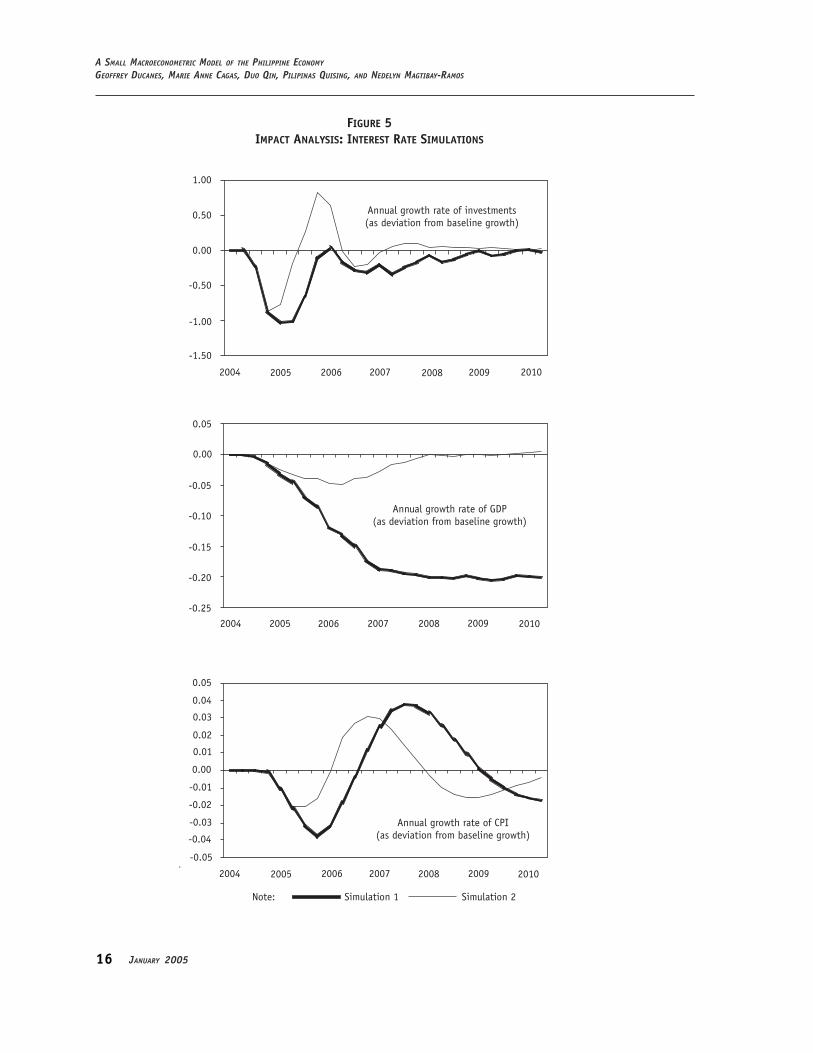
Figure 5 shows the effect of the interest rate shock on investments, GDP, and inflation. Notethat in the model investments depend negatively on the lending rate, which in turn follows themovement of the overnight borrowing rate. As the figure shows, the impulse shock reduces the growthrate of investments immediately after the shock although it recovers after about a year and thengrowth is higher than it would have been for about a year also, before finally tapering off. The effectof the step shock lingers but also erodes and, unlike in the impulse shock, there is no period whengrowth would have been significantly higher than it would have been without the shock.
The impulse shock lowers GDP growth very slightly for about 4 years (around 0.03 of a percentagepoint) before tapering off. The effect of the step shock is higher (average of slightly higher thanone tenth of one percentage point) and lingers before showing signs of leveling off at the end ofthe simulation period.
The impulse shock reduces inflation slightly compared to the base run for about a year afterthe shock, but this is short-lived as inflation becomes higher for about two years after that beforedeclining again and leveling off toward the end of the simulation period. The step shock reducesinflation initially for about two years but then inflation increases after that before declining again.
The effects of the interest rate hike on the real variables appear high, especially compared toa similar experiment done with ADB’s PRC model (see He et al. 2004). The high debt levels in the
8 The distribution should be approximately symmetric, as we have allowed for the use of antithetic stochastic shocks.For the detailed description of the stochastic simulations, see Pierse (2001).
9 This involved exogenizing the overnight borrowing rate, which is endogenous in the model.

13ERD WORKING PAPER SERIES NO. 62
2004 2005 2006 2007 2008 2009 2010Secondary sector value added
2004 2005 2006 2007 2008 2009 2010Primary sector value added
250000
200000
150000
100000
50000
0
350000
300000
250000
200000
150000
0
100000
50000
2004 2005 2006 2007 2008 2009 2010Private consumption
2004 2005 2006 2007 2008 2009 2010Tertiary sector value added
50000045000040000035000030000025000020000015000010000050000
0
800000
700000
600000
500000
300000200000100000
0
400000
2004 2005 2006 2007 2008 2009 2010Imports
350000
300000
250000
200000
150000
100000
50000
02004 2005 2006 2007 2008 2009 2010
Investments
200000
150000
100000
50000
0
250000
2004 2005 2006 2007 2008 2009 2010Employed
500004500040000350003000025000200001500010000
05000 -1000
-500
500
1500200025003000
0
2004 2005 2006 2007 2008 2009 2010-1500
1000
Current account balance
Note: 2% quantile 50% quantile 97% quantile
FIGURE 3STOCHASTIC SIMULATION RESULTS: SELECTED REAL SECTOR VARIABLES
See Appendix A for the variable units.
SECTION IVSIMULATION EXPERIMENTS

14 JANUARY 2005
A SMALL MACROECONOMETRIC MODEL OF THE PHILIPPINE ECONOMY
GEOFFREY DUCANES, MARIE ANNE CAGAS, DUO QIN, PILIPINAS QUISING, AND NEDELYN MAGTIBAY-RAMOS
1
2004 2005 2006 2007 2008 2009 2010Government expenditure
2004 2005 2006 2007 2008 2009 2010Government revenue
2004 2005 2006 2007 2008 2009 2010Foreign debt
2004 2005 2006 2007 2008 2009 2010Domestic debt
2004 2005 2006 2007 2008 2009 2010Net foreign assets
2004 2005 2006 2007 2008 2009 2010Money supply (M1)
2004 2004CPI
2005 2006 2007 2007 2008 2009 2010 20102004 2004 2005 2006 2007 2007 2008 2009 2010 2010GDP deflator
600000
500000
400000
300000
200000
100000
0
4500000400000035000003000000
2000000
1000000
0
2500000
1500000
500000
600000
500000
400000
300000
200000
100000
0
4000000
3500000
30000002500000
1500000
500000
0
2000000
1000000
1000000
600000
1200000
800000
400000
200000
0
1400000
1000000
1600000
1200000
800000600000400000200000
0-200000-400000
3
2.5
2
1.5
1
0.5
0
3.0
2.5
2.0
1.5
1.0
0.5
0.0
FIGURE 4STOCHASTIC RESULTS: SELECTED FISCAL, MONETARY AND PRICE VARIABLES
Note: 2% quantile 50% quantile 97% quantile
See Appendix A for the variable units.

15ERD WORKING PAPER SERIES NO. 62
country and persistent public deficits may account for this. Favero and Giavazzi (2003) in the caseof Brazil suggest that when the country’s fundamentals are weak and the risk of default high,monetary policy can have perverse effects. Following their framework and applying it to thePhilippines with modifications, the mechanism can be described as follows: With a significant portionof the public debt short term, an increase by the central bank of its benchmark rate raises domesticdebt service payments. As budget deficits continue, the debt level further rises and so does therisk of default. This results in a higher risk perception and higher interest rates on debts sourcedfrom abroad, and thus even higher debt, especially if currency depreciation also occurs. Investmentsalso decline as a result of the higher risk. The currency depreciation exerts inflationary pressure,which would cause the central bank to further raise interest rates, and so on. The result is a lingeringand even perverse (higher inflation) effect of an interest rate hike.
2. Fiscal Simulations
As noted above, the fiscal situation is deemed most critical for the Philippine economy. Thecentral government debt-to-GDP ratio is at an all-time high of about 78 percent, and with no immediatesolution to the chronic budget deficit, it is feared a fiscal crisis is looming. Very high debt levelsaffect the country negatively on several fronts. First, it raises the perceived risk of default of thecountry and as a result, investments go down. Second, higher debt levels mean increasingly higherinterest payment allocations by the government and thus lower allocation for other more importantitems such as infrastructure and social expenditures. These are reflected in the model.
Two simulation scenarios, illustrating two ways the government could address the budget deficitproblem, are run and compared to the base run where the government is assumed to just continueon its current path.
(i) Simulation Scenario 1: Government sets an upper-bound limit for the debt-to-GDPratio of 70 percent and for the government deficit to GDP ratio of 4 percent.10
The government reacts to a breach of either of these upper bounds by reducinggovernment noninterest payment expenditure by the fraction of the excess, or incase both are breached by the fraction of the higher excess. For instance, ifgovernment deficit for a quarter is 6 percent of GDP and the debt-to-GDP ratio isless than 70 percent, then government expenditure in the following quarter is reducedby 2 percent.
(ii) Simulation Scenario 2: In addition to what is in Scenario 1, the government is alsoable to maintain an annual increase in tax collection of 15 percent. This is notunreasonably high as figures higher than these have been achieved in the mid-1990s, moreover, tax efficiency is so low that there is a very large room forimprovement.
Figure 6 shows the evolution of the debt-to-GDP ratio under the base run and the twoalternative simulation scenarios as well as the effect of the two simulations on GDP growth andinvestment growth. As the dashed lines in the second graph show, GDP growth would be initially(slightly) lower when government expenditure is reduced as a response to too-high debt or deficit
10 The model allows for these bounds to be easily adjusted.
SECTION IVSIMULATION EXPERIMENTS
16 JANUARY 2005
A SMALL MACROECONOMETRIC MODEL OF THE PHILIPPINE ECONOMY
GEOFFREY DUCANES, MARIE ANNE CAGAS, DUO QIN, PILIPINAS QUISING, AND NEDELYN MAGTIBAY-RAMOS
.
Annual growth rate of investments(as deviation from baseline growth)
1.00
0.50
0.00
-0.50
-1.00
-1.50
2004 2005 2006 2007 2008 2009 2010
Annual growth rate of GDP(as deviation from baseline growth)
2004 2005 2006 2007 2008 2009 2010
0.05
0.00
-0.05
-0.10
-0.15
-0.20
-0.25
2004 2005 2006 2007 2008 2009 2010.
0.05
0.03
0.01
0.00
-0.02
-0.03
-0.05
Annual growth rate of CPI(as deviation from baseline growth)
0.04
0.02
-0.01
-0.04
FIGURE 5IMPACT ANALYSIS: INTEREST RATE SIMULATIONS
Note: Simulation 1 Simulation 2

17ERD WORKING PAPER SERIES NO. 62
Debt-to-GDP ratio
2004 2005 2006 2007 2008 2009 2010
0.86
0.84
0.82
0.80
0.78
0.76
0.74
0.72
0.70
0.68
2004 2005 2006 2007 2008 2009 2010
0.20
0.15
0.10
0.05
0.00
-0.05
1.00
0.80
0.60
0.40
0.20
0.00
-0.20
-0.40
-0.60
Annual growth rate of GDP(as deviation from base-run growth rate)
Annual growth rate of Investments(as deviation from base-run growth rate)
2004 2005 2006 2007 2008 2009 2010
FIGURE 6IMPACT ANALYSIS: FISCAL SIMULATIONS
Note: Base Simulation 1 Simulation 2
SECTION IVSIMULATION EXPERIMENTS

18 JANUARY 2005
A SMALL MACROECONOMETRIC MODEL OF THE PHILIPPINE ECONOMY
GEOFFREY DUCANES, MARIE ANNE CAGAS, DUO QIN, PILIPINAS QUISING, AND NEDELYN MAGTIBAY-RAMOS
but then afterward becomes significantly higher. At the end of the forecast period GDP growthis about 0.15 of a percentage point higher. Under Scenario 2, when an increase in tax collectionaccompanies the reduction in expenditure, GDP growth is even initially slightly lower than in Scenario1 but then also catches up and becomes much higher than base growth although not as high asin Scenario 1.11 These show the importance of reining in the government’s deficit problems. Theincrease in GDP growth under the two scenarios can be traced primarily to the increase in investmentsfor most of the period as shown in the last graph.
3. Oil Price Shock
As a final simulation exercise, we look at the effects of both impulse and step oil price shocksto the economy. The Philippines, being a small open economy highly dependent on oil imports, isseen as highly vulnerable to drastic upward swings in world oil prices. The base run assumes thatBrent oil price per barrel is at $45 for 2004Q4 and then declines to $35 per barrel by 2005Q1 up tothe end of the simulation period. The impulse shock assumes the $45 dollar per barrel lasts fortwo quarters from 2004Q4 to 2005Q1 then down to $35 per barrel in Q22005 up to the end of thesimulation period, while the step shock assumes the $45 dollar per barrel is constant from Q42004to the end of the simulation period.
Figure 7 shows the effects of the oil shocks to GDP growth, inflation, and private consumption.The impulse shock reduces GDP growth by about a fifth of a percentage point for about a year afterthe shock before tapering off. The step shock reduces GDP growth by an average of about six tenthsof a percentage point up to the end of the simulation period.
The impulse shock increases inflation by about a tenth of a percentage point for three yearsbefore tapering off. The effect of the step shock is much larger and pervasive, reaching a high ofalmost two percentage points before settling at about a third of a percentage point by the end ofthe simulation period. The average increase in inflation for the entire simulation period due to thestep shock is 0.55 percentage point.
The impulse shock reduces private consumption growth slightly by about a tenth of a percentagepoint for about 3 years before tapering off. However, the step shock has a huge effect on privateconsumption growth, cutting it increasingly until it settles at about half a percentage point at theend of the simulation period.
V. CONCLUSION
This paper describes an ADB quarterly macroeconometric model of the Philippines. The modelexhibits a number of desirable properties that the authors believe accords it distinct advantageover other existing macroeconometric models of the Philippines. During the modeling process,great efforts have been made to try to achieve the best possible blend of well-established a priorilong-run theories, short-run shock variables through a posteriori data guidance, and special features
11 The lower growth under Scenario 2 compared to Scenario 1 (at least up to 2010) can be attributed to the lowerprivate consumption growth that occurs in the former as disposable incomes decline because of higher taxes. Historically,private consumption has been a strong driving force of the Philippine economy.

19ERD WORKING PAPER SERIES NO. 62
-
FIGURE 7IMPACT ANALYSIS: OIL PRICE SIMULATIONS
Annual growth rate of GDP(as deviation from baseline growth)
0.20
0.10
0.00
-0.10
-0.20
-0.30
-0.40
-0.50
-0.60
-0.70
-0.80
Annual growth rate of CPI(as deviation from baseline growth)
2.00
1.50
1.00
0.50
0.00
-0.50
2004 2005 2006 2007 2008 2009 2010
2004 2005 2006 2007 2008 2009 2010
Annual growth rateof Private Consumption
(as deviation from baseline growth)
2004 2005 2006 2007 2008 2009 2010
0.10
0.10
-0.10
-0.20
-0.30
-0.40
-0.50
-0.60
-0.70
-0.80
Note: Impulse Step
SECTION VCONCLUSION

20 JANUARY 2005
A SMALL MACROECONOMETRIC MODEL OF THE PHILIPPINE ECONOMY
GEOFFREY DUCANES, MARIE ANNE CAGAS, DUO QIN, PILIPINAS QUISING, AND NEDELYN MAGTIBAY-RAMOS
of the Philippine economy. The resulting model demonstrates good forecasting capacity and versatilepotential for policy simulations.
The satisfactory within-sample forecasting capacity of the model is illustrated by conventionalmeasures of the predictive accuracy of the model such as root mean square percentage error andmean absolute percentage error, which were computed for several key variables in both static anddynamic runs of the model. The out-of-sample forecasting capacity of the model is illustrated bythe reasonably narrow uncertainty bands of the forecasts generated by stochastic simulations.
The policy simulation potential of the model is illustrated by three types of simulations: interestrate shocks, fiscal policy shocks, and world oil price shocks. The first set of simulations shows theimportance of maintaining a low interest rate regime in the country. The second set of simulationsshows that addressing the deficit and debt problems is very important if the Philippine governmenthopes to achieve and maintain higher growth of its economy in the medium and longer term. Theoil price simulations show the vulnerability of the Philippine economy to external shocks.

21ERD WORKING PAPER SERIES NO. 62
APPENDIX
APPENDIXSPECIFICATION AND STRUCTURE OF THE MODEL
A. List of Variables
1. Endogenous Variables
Consumption block
PCONc_PHI Private consumption in constant price (million 1994 pesos)PCON_PHI Private consumption in current price (million pesos)
Investment block
INVc_PHI Investments in constant price (million 1994 pesos)STKc_PHI Inventories in constant price (million 1994 pesos)STK_PHI Inventories in current price (million pesos)
Government block
GREV_PHI Government total revenue (million pesos)GTAX_PHI Government tax revenue (million pesos)GCON_PHI Government consumption in current price (million pesos)GCONc_PHI Government consumption in constant price (million 1994 pesos)GPAY_PHI Government expenditure less interest payments (million pesos)GINT_PHI Government interest payments (million pesos)DDEBT_PHI Domestic debt (million pesos)FDEBT_PHI Foreign debt (million pesos)
Trade block
X$_PHI Exports (million US dollars)M_PHI Imports (million pesos)CAB$_PHI Current account balance (million US dollars)
Production block
GDPcLR_PHI Long-run supply trend of constant GDP (million 1994 pesos)VA1c_PHI Value added of primary sector in constant price (million 1994 pesos)VA1_PHI Value added of primary sector in current price (million pesos)VA2c_PHI Value added of secondary sector in constant price (million 1994 pesos)VA2_PHI Value added of secondary sector in current price (million pesos)VA3c_PHI Value added of tertiary sector in constant price (million 1994 pesos)VA3_PHI Value added of tertiary sector in current price (million pesos)NFIA_PHI Net factor income from abroad in current price (million pesos)GNPc_PHI Gross national product in constant price (million 1994 pesos)
22 JANUARY 2005
A SMALL MACROECONOMETRIC MODEL OF THE PHILIPPINE ECONOMY
GEOFFREY DUCANES, MARIE ANNE CAGAS, DUO QIN, PILIPINAS QUISING, AND NEDELYN MAGTIBAY-RAMOS
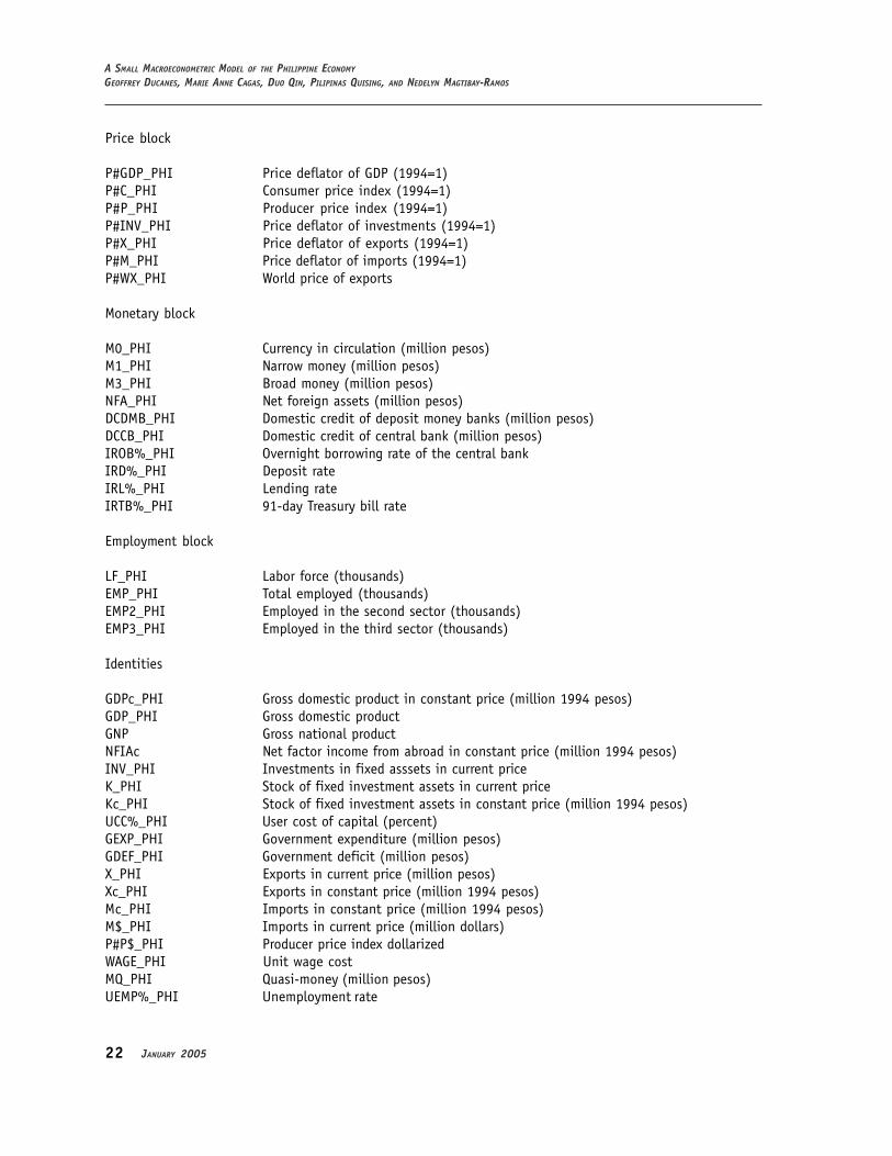
Price block
P#GDP_PHI Price deflator of GDP (1994=1)P#C_PHI Consumer price index (1994=1)P#P_PHI Producer price index (1994=1)P#INV_PHI Price deflator of investments (1994=1)P#X_PHI Price deflator of exports (1994=1)P#M_PHI Price deflator of imports (1994=1)P#WX_PHI World price of exports
Monetary block
M0_PHI Currency in circulation (million pesos)M1_PHI Narrow money (million pesos)M3_PHI Broad money (million pesos)NFA_PHI Net foreign assets (million pesos)DCDMB_PHI Domestic credit of deposit money banks (million pesos)DCCB_PHI Domestic credit of central bank (million pesos)IROB%_PHI Overnight borrowing rate of the central bankIRD%_PHI Deposit rateIRL%_PHI Lending rateIRTB%_PHI 91-day Treasury bill rate
Employment block
LF_PHI Labor force (thousands)EMP_PHI Total employed (thousands)EMP2_PHI Employed in the second sector (thousands)EMP3_PHI Employed in the third sector (thousands)
Identities
GDPc_PHI Gross domestic product in constant price (million 1994 pesos)GDP_PHI Gross domestic productGNP Gross national productNFIAc Net factor income from abroad in constant price (million 1994 pesos)INV_PHI Investments in fixed asssets in current priceK_PHI Stock of fixed investment assets in current priceKc_PHI Stock of fixed investment assets in constant price (million 1994 pesos)UCC%_PHI User cost of capital (percent)GEXP_PHI Government expenditure (million pesos)GDEF_PHI Government deficit (million pesos)X_PHI Exports in current price (million pesos)Xc_PHI Exports in constant price (million 1994 pesos)Mc_PHI Imports in constant price (million 1994 pesos)M$_PHI Imports in current price (million dollars)P#P$_PHI Producer price index dollarizedWAGE_PHI Unit wage costMQ_PHI Quasi-money (million pesos)UEMP%_PHI Unemployment rate
23ERD WORKING PAPER SERIES NO. 62
EMP1_PHI Employed in the primary sector (thousands)TDEBTr_PHI Total debt-to-GDP ratio of previous yearGDEFr_PHI Government deficit-to-GDP ratio of previous yearTEFT%_PHI Tax effort ratio of previous yearBEFT%_PHI Base tax effort ratio
2. Exogenous Variables
DEPK%_PHI Annual depreciation rate of fixed assetsER_PHI Peso-dollar exchange rateIRL%_USA US lending rateP#C_USA Consumer price index, USP#OIL$ Brent oil price spot rate (US dollars per barrel)P#WX$ World export price index dollarizedPOP_PHI Population (thousands)RAIN_PHI Rainfall indexTAX%_PHI Tax rateWT$_PHI World imports from the Philippines
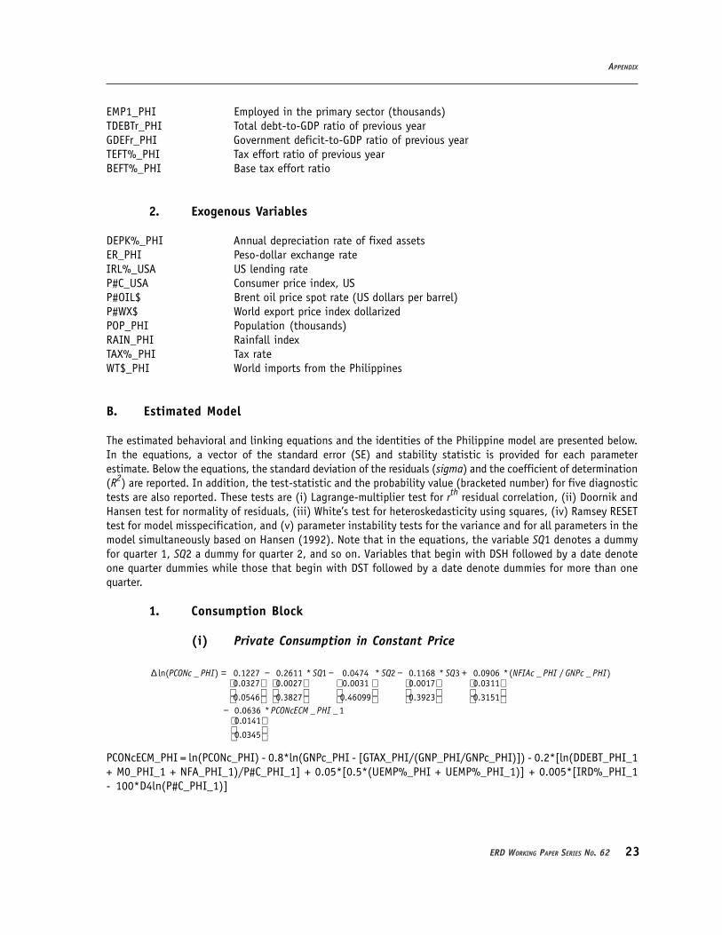
B. Estimated Model
The estimated behavioral and linking equations and the identities of the Philippine model are presented below.In the equations, a vector of the standard error (SE) and stability statistic is provided for each parameterestimate. Below the equations, the standard deviation of the residuals (sigma) and the coefficient of determination(R2) are reported. In addition, the test-statistic and the probability value (bracketed number) for five diagnostictests are also reported. These tests are (i) Lagrange-multiplier test for rth residual correlation, (ii) Doornik andHansen test for normality of residuals, (iii) White’s test for heteroskedasticity using squares, (iv) Ramsey RESETtest for model misspecification, and (v) parameter instability tests for the variance and for all parameters in themodel simultaneously based on Hansen (1992). Note that in the equations, the variable SQ1 denotes a dummyfor quarter 1, SQ2 a dummy for quarter 2, and so on. Variables that begin with DSH followed by a date denoteone quarter dummies while those that begin with DST followed by a date denote dummies for more than onequarter.
1. Consumption Block
(i) Private Consumption in Constant Price
∆ = − − − +
−
ln( _ ) 0.1227 0.2611 * 1 0.0474 * 2 0.1168 * 3 0.0906 *( _ / _ )0.0327 0.0027 0.0031 0.0017 0.0311
0.0546 0.3827 0.46099 0.3923 0.31510.0636 *0.0141
0.0345
PCONc PHI SQ SQ SQ NFIAc PHI GNPc PHI
P _ _ 1CONcECM PHI
PCONcECM_PHI = ln(PCONc_PHI) - 0.8*ln(GNPc_PHI - [GTAX_PHI/(GNP_PHI/GNPc_PHI)]) - 0.2*[ln(DDEBT_PHI_1+ M0_PHI_1 + NFA_PHI_1)/P#C_PHI_1] + 0.05*[0.5*(UEMP%_PHI + UEMP%_PHI_1)] + 0.005*[IRD%_PHI_1- 100*D4ln(P#C_PHI_1)]
APPENDIX

24 JANUARY 2005
A SMALL MACROECONOMETRIC MODEL OF THE PHILIPPINE ECONOMY
GEOFFREY DUCANES, MARIE ANNE CAGAS, DUO QIN, PILIPINAS QUISING, AND NEDELYN MAGTIBAY-RAMOS
sigma 0.0036R2 0.9988Autocorrelation F(3,29) = 3.1041 [0.0582]Normality Chi^2(2) = 1.4000 [0.4966]Homoscedasticity F(7,27) = 0.9004 [0.5205]RESET F(1,34) = 1.2779 [0.2662]Stability
variance 0.1049joint parameter constancy 2.4605
(ii) Private Consumption in Current Price
∆ = ∆ + ∆ + ∆
− ∆ −
ln( _ ) ln( _ ) 0.9779 * ln( # _ ) 0.0249 * ln( # _ _ 1)4 4 40.0179 0.0112
0.18345 0.09490.03345 * ln( # _ ) 0.1640 * _ _ 4
40.0091 0.0659
0.1784 0.4155
PCON PHI PCONc PHI P C PHI P M PHI
P M PHI PCONECM PHI
PCONECM_PHI = ln(PCON_PHI) - ln(PCONc_PHI) - 0.86*ln(P#C_PHI) - 0.07*ln(P#M_PHI_5)sigma 0.0049R2 —Autocorrelation F(3,36) = 0.5541 [0.6487]Normality Chi^2(2) = 0.6156 [0.7351]Homoscedasticity F(8,30) = 1.0293 [0.4363]RESET F(1,38) = 0.3620 [0.5510]Stability
variance 0.2813joint parameter constancy 1.0662
2. Investment Block
(i) Investment in Constant Price
∆ = − + ∆ − ∆ − + − −
− ∆ − − ∆ −
ln( _ ) 0.5198 1.1086 * ln( _ ) 0.3114 * [( _ ( 3) _ ( 3)) / _ ( 3)]30.1268 0.2078 0.0995
0.1926 0.1321 0.24140.0080 * [ % _ ( 1) ln( # (
40.0064
0.0381
INVc PHI GDPc PHI DDEBT PHI FDEBT PHI GDP PHI
IRL PHI P C −
1))] 0.3405 * _ _ 10.0878
0.1956
INVcECM PHI
INVcECM_PHI = ln(INVc_PHI) - ln(GDPc_PHI)
sigma 0.0578R2 0.6920Autocorrelation F(3,25) = 0.0918 [0.9640]Normality Chi^2(2) = 2.2117 [0.3309]Homoscedasticity F(6,21) = 0.5443 [0.8115]

25ERD WORKING PAPER SERIES NO. 62
RESET F(1,27) = 0.0684 [0.7953]Stability
variance 0.1133joint parameter constancy 0.8749
(ii) Inventories in Constant Price
∆ = + − ∆
− ∆ −
+
_ _ *[( _ _1 / _ _1)] 0.0297 0.4778 * ln( # _ _ 4)30.0061 0.0839
0.1768 0.11880.1034 * ln( _ ) 0.1889 * _ _1
30.0305 0.0498
0.1041 0.28390.16740.06
STKc PHI GDPc PHI STKc PHI GDPc PHI P GDP PHI
ER PHI STKcECM PHI
∆ + + + −
−+ ∆ + + + −
−
* [ln( _ _ 3 _ _ 3 _ _ 3 _ _ 3 _ _ 3)235
0.1306ln( _ _ 3)]0.1153 * [ln( _ _ 5 _ _ 5 _ _5 _ _5 _ _ 5)
20.0602
0.0722ln( _ _ 5)]
PCONc PHI GCONc PHI INVc PHI Xc PHI M PHI
GDPcLR PHIPCONc PHI GCONc PHI INVc PHI Xc PHI Mc PHI
GDPcLR PHI
STKcECM_PHI = STKc_PHI/GDPc_PHI - [ln(PCONc_PHI + GCONc_PHI + INVc_PHI + Xc_PHI -Mc_PHI) - ln(GDPcLR_PHI)]
sigma 0.0141R2 0.5884Autocorrelation F(3,27) = 0.3309 [0.8031]Normality Chi^2(2) = 0.4832 [0.7854]Homoscedasticity F(10,19) = 1.1909 [0.3553]RESET F(1,29) = 1.0383 [0.3167]Stability
variance 0.2123joint parameter constancy 1.2020
(iii) Inventories in Current Price
∆ = + ∆ −
_ 729.422 0.6698 * ( _ * # _ ) 1.1425 * _ _1478.3 0.0337 0.1671
0.1312 0.0965 0.2797
STK PHI STKc PHI P INV PHI STKECM PHI
STKECM_PHI = STK_PHI - 0.70*(STKc_PHI*P#INV_PHI)
sigma 2810.05R2 0.9349Autocorrelation F(3,30) = 0.4185 [0.7410]Normality Chi^2(2) = 0.4790 [0.7870]Homoscedasticity F(4,28) = 0.4600 [0.7644]RESET F(1,32) = 0.2639 [0.6110]Stability
variance 0.2023joint parameter constancy 0.6152
APPENDIX

26 JANUARY 2005
A SMALL MACROECONOMETRIC MODEL OF THE PHILIPPINE ECONOMY
GEOFFREY DUCANES, MARIE ANNE CAGAS, DUO QIN, PILIPINAS QUISING, AND NEDELYN MAGTIBAY-RAMOS
3. Government Block
(i) Government Revenue
∆ = + ∆ + −
ln( _ ) 0.1161 0.9347 * ln( _ ) 0.0316 * 2002 3 0.9745 * _ _ 10.0223 0.0431 0.1816 0.0161
0.0860 0.1432 0.1191 0.0682
GREV PHI GTAX PHI DST Q GREVECM PHI
GREVECM_PHI = ln(GREV_PHI) - ln(GTAX_PHI)
Sigma 0.0346R2 0.9442Autocorrelation F(3,25) = 1.3762 [0.2730]Normality Chi^2(2) = 3.8701 [0.1444]Homoscedasticity F(5,22) = 2.2084 [0.0900]RESET F(1,27) = 3.5454 [0.0705]Stability
variance 0.4598joint parameter constancy 1.3423
(ii) Government Tax Revenues
∆ = − − − +
+ ∆ + ∆
ln( _ ) 0.2710 *(ln( _ ) ln( _ _ 2)) 0.2110 * 1 0.1753 * 20.0929 0.0538 0.0279
0.06116 0.0807 0.05840.6448 * ln( _ ) 0.8331 * ln( _0.1097 0.3045
0.0374 0.0753
GTAX PHI GTAX PHI GTAX PHI SQ SQ
GNP PHI GNP
+ ∆ −
_ 1)
0.4470 * ln( _ _ 2) 0.5769 *0.1569 0.1023
0.1217 0.0513
PHI
GNP PHI GTAXECM
GTAXECM_PHI = ln(GTAX_PHI) - ln(GNP_PHI) - 0.095*TAX%_PHI +5.17
sigma 0.0333R2 —Autocorrelation F(3,22) = 0.5576 [0.6808]Normality Chi^2(2) = 2.9366 [0.2303]Homoscedasticity F(10,14) = 1.1246 [0.3831]RESET F(1,24) = 0.0946 [0.7600]Stability
variance 0.25084joint parameter constancy 1.6218

27ERD WORKING PAPER SERIES NO. 62
(iii) Government Tax Revenues (alternative)
= − − −
+ + ∆ +
ln( _ ) (200402)*(ln( _ _ 1) 0.2710 *(ln( _ ) ln( _ _ 2)) 0.2110 * 10.0929 0.0538
0.06116 0.08070.1753 * 2 0.6448 * ln( _ ) 0.83310.0279 0.1097
0.0584 0.0374
GTAX PHI ifle GTAX PHI GTAX PHI GTAX PHI SQ
SQ GNP PHI ∆ + ∆
− +
+ + +
* ln( _ _ 1) 0.4470 * ln( _ _ 2)0.3045 0.1569
0.0753 0.12170.5769 * ) ( 2004 2)* ln(( % _ _ 4 / % _ )^ (1 / )*0.1023
0.0513( _ _ 1 _ _ 2 _ _ 3 _ _ 4)
GNP PHI GNP PHI
GTAXECM DST Q TAX PHI BEFT PHI YRStxGAP
GDP PHI GDP PHI GDP PHI GDP PHI ++ + +
/( _ _ 5 _ _ 6_ _7 _ _ 8))) ln( _ _ 4)
GDP PHI GDP PHIGDP PHI GDP PHI GTAX PHI
GTAXECM_PHI = ln(GTAX_PHI) - ln(GNP_PHI) - 0.095*TAX%_PHI +5.17
4. Government Consumption in Current Price
∆ = ∆ − + ∆ −
−
ln( _ ) 0.5480 * ln( _ _1) 0.0997 0.2911 * ln( _ ) 0.0312 * 2003 34 4 40.1074 0.0285 0.0779 0.0173
0.1672 0.2012 0.1882 0.01160.5896 * _ _ 40.1255
0.1096
GCON PHI GCON PHI GPAY PHI DST Q
GCONECM PHI
GCONECM_PHI = ln(GCON_PHI) - ln(GPAY_PHI)
Sigma 0.0321R2 0.8118Autocorrelation F(3,20) = 1.1620 [0.3489]Normality Chi^2(2) = 0.6760 [0.3201]Homoscedasticity F(7,15) = 0.2606 [0.9602]RESET F(1,22) = 0.2826 [0.6004]Stability
variance 0.2242joint parameter constancy 1.1232
(i) Government Noninterest Payment Expenditure
= + + ∆ + ∆
−
ln( _ ) [ln( _ _ 4) 0.0825 0.6166 * ln( _ ) 0.0227 * % _ _ 34 20.0161 0.1572 0.0063
0.0965 0.1998 0.07360.9088 * _ _ 4]0.1448
0.0795
GPAY PHI GPAY PHI GREV PHI UEMP PHI
GPAYECM PHI
GPAYECM_PHI = ln(GPAY_PHI) - ln(GREV_PHI)+ 0.24*[(DDEBT_PHI_4+FDEBT_PHI_4)/GNP_PHI_4] - 0.04*UEMP%_PHI_1
APPENDIX

28 JANUARY 2005
A SMALL MACROECONOMETRIC MODEL OF THE PHILIPPINE ECONOMY
GEOFFREY DUCANES, MARIE ANNE CAGAS, DUO QIN, PILIPINAS QUISING, AND NEDELYN MAGTIBAY-RAMOS
sigma 0.0703R2 0.6128Autocorrelation F(3,25) = 0.8108 [0.4999]Normality Chi^2(2) = 4.9365 [0.0847]Homoscedasticity F(6,21) = 0.2500 [0.9538]RESET F(1,27) = 0.4187 [0.5230]Stability
variance 0.2765joint parameter constancy 0.9869
(ii) Government Noninterest Payment Expenditure (alternative)
ln( _ ) [ln( _ _ 4) 0.0825 0.6166 * ln( _ ) 0.0227 * % _ _ 34 20.0161 0.1572 0.0063
0.0965 0.1998 0.07360.9088 * _ _ 4] ( 2004 2)*min[1,( _0.1448
0.0795
GPAY PHI GPAY PHI GREV PHI UEMP PHI
GPAYECM PHI DST Q TDEBTr P
= + + ∆ + ∆
− +
0.75 _ 0.04)]
*log[1 0.25*max( _ 0.75, _ 0.04)])
HI GDEFr PHI
TDEBTr PHI GDEFr PHI
− + +
− − − −
GPAYECM_PHI = ln(GPAY_PHI) - ln(GREV_PHI)+ 0.24*[(DDEBT_PHI_4+FDEBT_PHI_4)/GNP_PHI_4] - 0.04*UEMP%_PHI_1
5. Government Interest Payment Expenditure
_ *1000.0283 * _ 0.0394 * % _ 0.2107 * 3
_ _ 0.0013 0.0064 0.0639
0.1395 0.1699 0.0962
GINT PHIER PHI IRTB PHI SQ
DDEBT PHI FDEBT PHI= + +
+
sigma 0.1376R2 —Autocorrelation F(3,36) = 0.4748 [0.7033]Normality Chi^2(2) = 4.7449 [0.0933]Homoscedasticity F(4,34) = 0.9600 [0.4691]RESET F(1,38) = 0.1527 [0.6997]Stability
variance 0.4417joint parameter constancy 0.9410
6. Domestic Debt
2 _ 7388.86 1.4700 * _ _ 1 1.1947 * _ _13828.0 0.3093 0.1556
0.2604 0.2070 0.31198489.14 * [0.25*( % _ _ 3 % _ _ 4 % _ _ 5 % _ _ 6)]4462.0
0.3979
DDEBT PHI GDEF PHI DDEBTECM PHI
IRTB PHI IRTB PHI IRTB PHI IRTB PHI
∆ = + ∆ −
+ ∆ + + +

29ERD WORKING PAPER SERIES NO. 62
DDEBTECM_PHI = ∆DDDEBT_PHI + GDEF_PHI_1
sigma 21355.9R2 0.7076Autocorrelation F(3,27) = 1.0733 [0.3769]Normality Chi^2(2) = 0.2554 [0.9945]Homoscedasticity F(6,23) = 1.6129 [0.1887]RESET F(1,29) = 0.1523 [0.6992]Stability
variance 0.0785joint parameter constancy 1.0005
7. Foreign Debt
2 2_ 7638.41 15125 * _ 5504.4 * ( % _ % _ ) 54321.7 * % _6351.0 3168.0 4455.0 16900
0.0758 0.0463 0.3332 0.06941.74598 * _ _10.1972
0.0859
FDEBT PHI ER PHI IRL PHI IRL USA IRL USA
FDEBTECM PHI
∆ = + ∆ + ∆ − + ∆
−
FDEBTECM_PHI = ∆DFDEBT_PHI + GDEF_PHI - 10021*∆ER_PHIsigma 35268.6R2 0.7527Autocorrelation F(3,26) = 0.4736 [0.7033]Normality Chi^2(2) = 5.0872 [0.0786]Homoscedasticity F(8,20) = 0.3681 [0.9253]RESET F(1,28) = 1.3708 [0.2515]Stability
variance 0.1090joint parameter constancy 0.7842
8. Government Consumption in Constant Price
ln( _ ) ln( _ ) ln( _ _ 1 / _ _ 1) 0.1968 0.3537 * 1 0.1571 * 20.0141 0.0333 0.0133
0.24555 0.1897 0.13280.13397 * 3 1.7417 * ln( 30.0155 0.4602
0.1581 0.2078
GCONc PHI GCON PHI GCON PHI GCONc PHI SQ SQ
SQ VA
= − − + +
+ − ∆
_ / 3 _ ) 0.3970 * _ _ 10.1167
0.1943
PHI VA c PHI GCONcECM PHI+
GCONcECM_PHI = ln(GCON_PHI) - ln(GCONc_PHI) - ln(VA3_PHI/VA3c_PHI)
sigma 0.0279R2 —Autocorrelation F(4,34) = 1.7646 [0.1725]Normality Chi^2(2) = 0.1828 [0.9127]Homoscedasticity F(6,30) = 2.7377 [0.0305]*RESET F(1,36) = 8.5123 [0.0060]**
APPENDIX

30 JANUARY 2005
A SMALL MACROECONOMETRIC MODEL OF THE PHILIPPINE ECONOMY
GEOFFREY DUCANES, MARIE ANNE CAGAS, DUO QIN, PILIPINAS QUISING, AND NEDELYN MAGTIBAY-RAMOS
Stabilityvariance 0.1937joint parameter constancy 1.6331**
D. Trade Block
1. Exports
ln( $ _ ) 0.0527 0.7389 * ln( $ _ ) 0.1727 * 90 197 4 0.1068 * 00 110 40.0236 0.0932 0.0323 0.0313
0.0949 0.3133 0.0397 0.15910.5786 *(ln( $ _ _ 1) ln( $ _ _ 1))0.1046
0.0690
X PHI WT PHI DST Q Q DST Q Q
X PHI WT PHI
= + + −
− −
sigma 0.0496R2 0.7058Autocorrelation F(3,20) = 0.3425 [0.8474]Normality Chi^2(2) = 0.5798 [0.7483]Homoscedasticity F(5,17) = 0.4233 [0.8581]RESET F(1,22) = 0.0559 [0.8143]Stability
variance 0.1293joint parameter constancy 1.0285
2. Imports
ln( _ ) 0.2730 0.1707 * ln( _ ) 0.5040 * ln( _ ) 0.6095 * _ _ 150.0601 0.0919 0.1391 0.1378
0.2073 0.0877 0.1529 0.17880.4228 * ln( _ _ 2 _ _ 2
20.2110
0.2303
M PHI X PHI X PHI MECM PHI
PCON PHI GCON PHI IN
∆ = − + ∆ + ∆ −
+ ∆ + +
_ _ 2)V PHI
MECM_PHI = ln(M_PHI) - 0.6*ln(X_PHI) - 0.4*ln(PCON_PHI+GCON_PHI+INV_PHI) -6*[P#P_PHI/(P#WX$_PHI*ER_PHI)]
sigma 0.0631R2 0.6446Autocorrelation F(3,28) = 0.7928 [0.5082]Normality Chi^2(2) = 4.2113 [0.1218]Homoscedasticity F(8,22) = 0.5447 [0.8103]RESET F(1,30) = 0.6133 [0.4397]Stability
variance 0.1231joint parameter constancy 0.8399

31ERD WORKING PAPER SERIES NO. 62
3. Current Account Balance
$ _ 281.602 0.9578 * ln( $ _ $ _ ) 0.6937 * $ _ _194.360 0.0801 0.1777
0.1311 0.1144 0.1373
CAB PHI X PHI M PHI CAB ECM PHI∆ = + ∆ − −
CAB$ECM_PHI = CAB$_PHI - (X$_PHI - M$_PHI)
sigma 382.196R2 0.8278Autocorrelation F(3,27) = 1.4714 [0.2445]Normality Chi^2(2) = 5.5125 [0.0635]Homoscedasticity F(4,25) = 0.6799 [0.6124]RESET F(1,29) = 0.9634 [0.3344]Stability
variance 0.2082joint parameter constancy 0.5228
E. Production Block
1. Long-run Supply Trend of GDP in Constant Price
ln( _ ) 0.95 0.0689* ln( ) 0.64 * ln( _ ) 0.36* ln( _ ) 0.0286* (2000 1)GDPcLR PHI TIME EMP PHI Kc PHI DST Q= + + + +
2. Value Added in the Primary Sector in Constant Price
ln( 1 _ ) 0.8101 0.0916 * ln( _ _ 1) 1.8134 * ln( 3 _ _1) 0.2418 * ln( 3 _ _ 4)4 4 40.1095 0.0081 0.3485 0.0430
0.0870 0.1660 0.1013 0.10970.0664 * ln( 2
30.0363
0.1012
VA c PHI RAIN PHI VA c PHI VA c PHI
VA c
∆ = − + ∆ + ∆ + ∆
+ ∆
_ _2) 0.2469 * 1 _ _ 40.0356
0.0866
PHI VA cECM PHI−
VA1cECM_PHI = ln(VA1c_PHI) - 0.31*ln(RAIN_PHI_1) - ln(VA2c_PHI_1 + VA3c_PHI_1)
sigma 0.0195R2 0.8411Autocorrelation F(3,23) = 1.0295 [0.3980]Normality Chi^2(2) = 0.5826 [0.7473]Homoscedasticity F(10,15) = 0.8513 [0.5920]RESET F(1,25) = 1.3205 [0.2614]Stability
variance 0.1251joint parameter constancy 0.9690
APPENDIX
32 JANUARY 2005
A SMALL MACROECONOMETRIC MODEL OF THE PHILIPPINE ECONOMY
GEOFFREY DUCANES, MARIE ANNE CAGAS, DUO QIN, PILIPINAS QUISING, AND NEDELYN MAGTIBAY-RAMOS
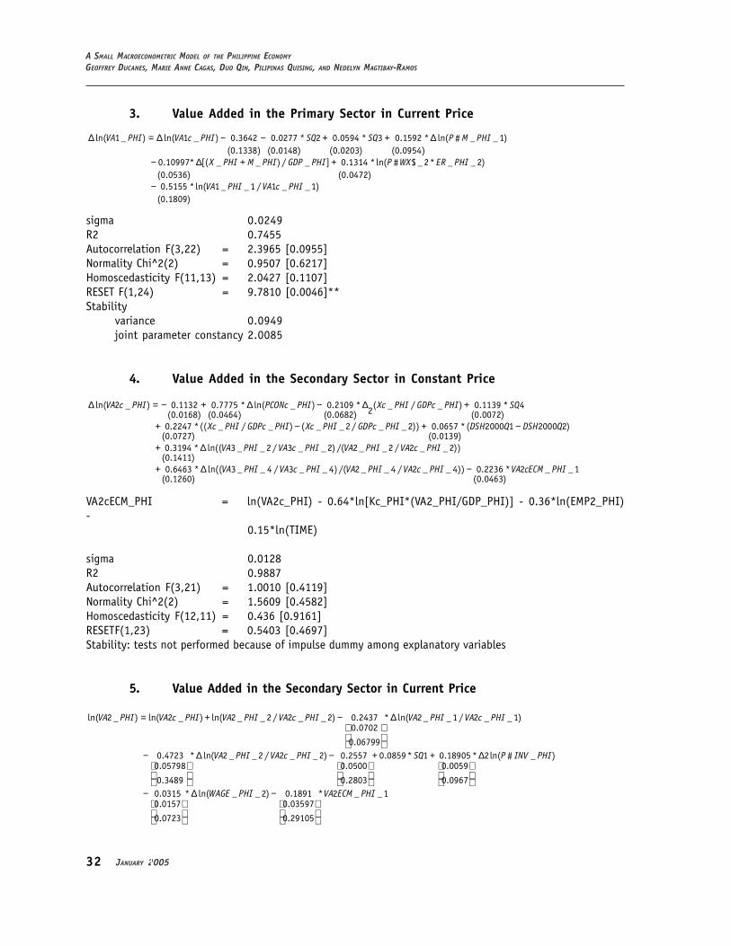
3. Value Added in the Primary Sector in Current Price
ln( 1 _ ) ln( 1 _ ) 0.3642 0.0277 * 2 0.0594 * 3 0.1592 * ln( # _ _ 1)(0.1338) (0.0148) (0.0203) (0.0954)
0.10997* [( _ _ ) / _ ] 0.1314 * ln( # $ _ 2* _ _ 2)(0.0536) (0.0472)0.5155
(0.1809
VA PHI VA c PHI SQ SQ P M PHI
X PHI M PHI GDP PHI P WX ER PHI
∆ = ∆ − − + + ∆
− ∆ + +
− * ln( 1 _ _ 1 / 1 _ _1))
VA PHI VA c PHI
sigma 0.0249R2 0.7455Autocorrelation F(3,22) = 2.3965 [0.0955]Normality Chi^2(2) = 0.9507 [0.6217]Homoscedasticity F(11,13) = 2.0427 [0.1107]RESET F(1,24) = 9.7810 [0.0046]**Stability
variance 0.0949joint parameter constancy 2.0085
4. Value Added in the Secondary Sector in Constant Price
ln( 2 _ ) 0.1132 0.7775 * ln( _ ) 0.2109 * ( _ / _ ) 0.1139 * 42(0.0168) (0.0464) (0.0682) (0.0072)
0.2247 *(( _ / _ ) ( _ _ 2 / _ _ 2)) 0.0657 *( 2000 1(0.0727) (0.0139)
VA c PHI PCONc PHI Xc PHI GDPc PHI SQ
Xc PHI GDPc PHI Xc PHI GDPc PHI DSH Q DSH
∆ = − + ∆ − ∆ +
+ − + − 2000 2)
0.3194 * ln(( 3 _ _ 2 / 3 _ _ 2) /( 2 _ _2 / 2 _ _ 2))(0.1411)0.6463 * ln(( 3 _ _ 4 / 3 _ _ 4) /( 2 _ _ 4 / 2 _ _ 4)) 0.2236 * 2 _ _1
(0.1260) (0.0463)
Q
VA PHI VA c PHI VA PHI VA c PHI
VA PHI VA c PHI VA PHI VA c PHI VA cECM PHI
+ ∆
+ ∆ −
VA2cECM_PHI = ln(VA2c_PHI) - 0.64*ln[Kc_PHI*(VA2_PHI/GDP_PHI)] - 0.36*ln(EMP2_PHI)-
0.15*ln(TIME)
sigma 0.0128R2 0.9887Autocorrelation F(3,21) = 1.0010 [0.4119]Normality Chi^2(2) = 1.5609 [0.4582]Homoscedasticity F(12,11) = 0.436 [0.9161]RESETF(1,23) = 0.5403 [0.4697]Stability: tests not performed because of impulse dummy among explanatory variables
5. Value Added in the Secondary Sector in Current Price
ln( 2 _ ) ln( 2 _ ) ln( 2 _ _ 2 / 2 _ _ 2) 0.2437 * ln( 2 _ _1 / 2 _ _ 1)0.0702
0.067990.4723 * ln( 2 _ _ 2 / 2 _ _ 2) 0.2557 0.0859* 1 0.189050.05798 0.0500 0.0
0.3489 0.2803
VA PHI VA c PHI VA PHI VA c PHI VA PHI VA c PHI
VA PHI VA c PHI SQ
= + − ∆
− ∆ − + +
* 2ln( # _ )059
0.09670.0315 * ln( _ _ 2) 0.1891 * 2 _ _10.0157 0.03597
0.0723 0.29105
P INV PHI
WAGE PHI VA ECM PHI
∆
− ∆ −

33ERD WORKING PAPER SERIES NO. 62
VA2ECM_PHI = ln(VA2_PHI) - ln(VA2c_PHI) - 0.65*ln(P#INV_PHI) - 0.2*ln(P#M_PHI_1) -0.15*ln(WAGE_PHI)
sigma 0.0120R2 0.9393Autocorrelation F(3,31) = 0.4225 [0.7382]Normality Chi^2(2) = 0.2705 [0.8735]Homoscedasticity F(11,22) = 0.4715 [0.9014]RESET F(1,33) = 1.2670 [0.2684]Stability
variance 0.1623joint parameter constancy 1.2881
6. Value Added in the Tertiary Sector in Constant Price
ln( 3 _ ) 0.0328 0.2501 * 1 0.0453 * 2 0.0993 * 3 0.0161 * 2000 4(0.0261) (0.0102) (0.0039) (0.0038) (0.0040)0.0074 * 2001 1 0.1911 * ln[ _ /( 2 _ / 2 _ )]
(0.0042) (0.0324)0.0324 *
(0.0068)
VA c PHI SQ SQ SQ DSH Q
DSH Q GNP PHI VA PHI VA c PHI
∆ = − − − − −
+ + ∆
− ∆ ln[( 1 _ / 1 _ ) /( 2 _ / 2 _ )]2
0.1016 * ln[( 3 _ / 3 _ ) /( 2 _ / 2 _ )] 0.1177 * 3 _ _1(0.0388) (0.0212)
VA PHI VA c PHI VA PHI VA c PHI
VA PHI VA c PHI VA PHI VA c PHI VA cECM PHI− ∆ −
VA3cECM_PHI = ln(VA3c_PHI) - ln[GNP_PHI/(VA2_PHI/VA2c_PHI)] - 0.13*ln(TIME) +ln[(VA3_PHI/VA3c_PHI)/(VA2_PHI/VA2c_PHI)]
sigma 0.0038R2 0.9991Autocorrelation F(4,31) = 2.3908 [0.0721]Normality Chi^2(2) = 0.6292 [0.7301]Homoscedasticity F(13,21) = 0.5353 [0.8763]RESET F(1,34) = 3.1455 [0.0851]Stability: tests not performed because of impulse dummy among explanatory variables
7. Value Added in the Tertiary Sector in Current Price
ln( 3 _ ) ln( 3 _ ) 0.4286 * ln( 3 _ / 3 _ ) 0.0097 0.0653 * 1 0.0583 * 30.1144 0.00345 0.0037 0.0080
0.1291 0.15097 0.2502 0.18980.10550.04775
0.0869
VA PHI VA c PHI VA PHI VA c PHI SQ SQ
= + ∆ + + −
* ln( 2 _ _2 / 2 _ _ 2) 0.0424 * ln( # _ ) 0.0560 * _ _ 14 30.0131 0.0237
0.1631 0.0852
VA PHI VA c PHI P M PHI VA ECM PHI
∆ + ∆ −
VA3ECM_PHI = ln(VA3_PHI) - ln(VA3c_PHI) - ln(VA2_PHI_1/VA2c_PHI_1)sigma 0.0073R2 0.7121
APPENDIX

34 JANUARY 2005
A SMALL MACROECONOMETRIC MODEL OF THE PHILIPPINE ECONOMY
GEOFFREY DUCANES, MARIE ANNE CAGAS, DUO QIN, PILIPINAS QUISING, AND NEDELYN MAGTIBAY-RAMOS
Autocorrelation F(3,32) = 2.9901 [0.0455]*Normality Chi^2(2) = 1.1489 [0.5630]Homoscedasticity F(6,28) = 1.2151 [0.3280]RESET F(1,34) = 0.9546 [0.3355]Stability
variance 0.5793*joint parameter constancy 1.5135
8. Net Factor Income from Abroad in Current Price
( _ ) 0.6368 * _ _ 1 18808.2 10526.8* 1 7736.38* 2 12795.9* 200004(0.1107) (8554) (3103)(5007) (5454)
1353.62* % _ _ 2 0.0496 * _ _ 1(835.5) (0.0202)
NFIA PHI NFIA PHI SQ SQ DSH
UEMP PHI NFIAECM PHI
∆ = − ∆ − + + +
+ ∆ −
NFIAECM_PHI = NFIA_PHI - 38000*UEMP%_PHI
sigma 4717.1R2 0.6200Autocorrelation F(3,30) = 0.3319 [0.8023]Normality Chi^2(2) = 37.356 [0.0000]**Homoscedasticity F(9,23) = 0.6932 [0.7081]RESET F(1,32) = 0.0562 [0.8140]Stability: tests not performed because of impulse dummy among explanatory variables
9. Gross National Product in Constant Price
ln( _ ) ln( _ ) ( 0.0134 0.9914 * ln( # _ ) 0.0606 * 1 0.0094 * 30.0001 0.0097 0.0005 0.0002
0.0247 0.0898 0.0762 0.11900.1732 * _ _ 1)0.0060
0.1414
GNPc PHI GNP PHI P GDP PHI SQ SQ
GNPcECM PHI
= − + ∆ − +
−
GNPcECM_PHI = ln(GNP_PHI) - ln(GNPc_PHI) - 0.98326*ln(P#GDP_PHI)
sigma 0.0005R2 0.9984Autocorrelation F(3,26) = 2.2927 [0.1016]Normality Chi^2(2) = 4.4759 [0.1067]Homoscedasticity F(6,22) = 0.4358 [0.8470]RESET F(1,28) = 0.1031 [0.7506]Stability
variance 0.3947joint parameter constancy 0.8819
35ERD WORKING PAPER SERIES NO. 62
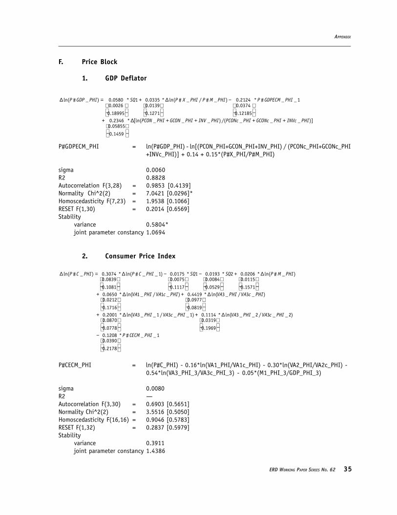
F. Price Block
1. GDP Deflator
ln( # _ ) 0.0580 * 1 0.0335 * ln( # _ / # _ ) 0.2124 * # _ _10.0026 0.0139 0.0374
0.18995 0.1271 0.121850.2346 * [ln( _ _ _ ) /( _0.05855
0.1459
P GDP PHI SQ P X PHI P M PHI P GDPECM PHI
PCON PHI GCON PHI INV PHI PCONc PHI
∆ = + ∆ −
+ ∆ + +
_ _ )]GCONc PHI INVc PHI+ +
P#GDPECM_PHI = ln(P#GDP_PHI) - ln[(PCON_PHI+GCON_PHI+INV_PHI) / (PCONc_PHI+GCONc_PHI+INVc_PHI)] + 0.14 + 0.15*(P#X_PHI/P#M_PHI)
sigma 0.0060R2 0.8828Autocorrelation F(3,28) = 0.9853 [0.4139]Normality Chi^2(2) = 7.0421 [0.0296]*Homoscedasticity F(7,23) = 1.9538 [0.1066]RESET F(1,30) = 0.2014 [0.6569]Stability
variance 0.5804*joint parameter constancy 1.0694
2. Consumer Price Index
ln( # _ ) 0.3074 * ln( # _ _ 1) 0.0175 * 1 0.0193 * 2 0.0206 * ln( # _ )0.0839 0.0075 0.0084 0.0115
0.1081 0.1117 0.0529 0.15710.0650 * ln( 1 _ / 1 _ ) 0.440.0212
0.1716
P C PHI P C PHI SQ SQ P M PHI
VA PHI VA c PHI
∆ = ∆ − − + ∆
+ ∆ +
19 * ln( 3 _ / 3 _ )0.0977
0.08190.2001 * ln( 3 _ _ 1 / 3 _ _1) 0.1114 * ln( 3 _ _ 2 / 3 _ _ 2)0.0870 0.0319
0.0778 0.19690.1208 * # _ _ 10.0390
0.2178
VA PHI VA c PHI
VA PHI VA c PHI VA PHI VA c PHI
P CECM PHI
∆
+ ∆ + ∆
−
P#CECM_PHI = ln(P#C_PHI) - 0.16*ln(VA1_PHI/VA1c_PHI) - 0.30*ln(VA2_PHI/VA2c_PHI) -0.54*ln(VA3_PHI_3/VA3c_PHI_3) - 0.05*(M1_PHI_3/GDP_PHI_3)
sigma 0.0080R2 —Autocorrelation F(3,30) = 0.6903 [0.5651]Normality Chi^2(2) = 3.5516 [0.5050]Homoscedasticity F(16,16) = 0.9046 [0.5783]RESET F(1,32) = 0.2837 [0.5979]Stability
variance 0.3911joint parameter constancy 1.4386
APPENDIX

36 JANUARY 2005
A SMALL MACROECONOMETRIC MODEL OF THE PHILIPPINE ECONOMY
GEOFFREY DUCANES, MARIE ANNE CAGAS, DUO QIN, PILIPINAS QUISING, AND NEDELYN MAGTIBAY-RAMOS
3. Producer Price Index
ln( # _ ) 0.1248 0.1451 * ln( # _ ) 0.2358 * ln( 1 _ / 1 _ )0.0325 0.0332 0.0514
0.0627 0.1259 0.34850.6201 * ln( 3 _ / 3 _ ) 0.2091 * #
40.1514 0.0557
0.0677 0.0727
P P PHI P M PHI VA PHI VA c PHI
VA PHI VA c PHI P P
∆ = − + ∆ + ∆
+ ∆ −
_ 0.2352 * ln( # _ _ 3)0.0429
0.1357
ECM PHI P INV PHI+ ∆
P#PECM_PHI = ln(P#P_PHI) - ln(VA2_PHI/VA2c_PHI)
sigma 0.0126R2 0.7311Autocorrelation F(3,22) = 0.5591 [0.6476]Normality Chi^2(2) = 3.9676 [0.1375]Homoscedasticity F(10,14) = 0.3491 [0.9500]RESET F(1,24) = 0.6748 [0.4195]Stability
variance 0.0452joint parameter constancy 1.4507
4. Investment Deflator
ln( # _ ) 0.0235 0.3544 * ln( 1 _ _ 1 / 1 _ _ 1) 0.4069 * ln( 3 _ / 3 _ )0.0056 0.0809 0.1131
0.2129 0.0822 0.22941.5749 * ln( 3 _ ( 1) / 3 _ ( 1)) 0.25090.1085
0.1208
P INV PHI VA PHI VA c PHI VA PHI VA c PHI
VA PHI VA c PHI
∆ = − + ∆ − ∆
+ ∆ − − −
* # _ _ 10.0754
0.0455
P INVECM PHI
P#INVECM_PHI = ln(P#INV_PHI) - 0.46*ln(VA2_PHI_2/VA2c_PHI_2) - 0.54*ln(VA2_PHI_2/VA2c_PHI_2) - 0.005*(0.25*[(IRL%_PHI_2 -100*∆4ln(P#C_PHI_2))+(IRL%_PHI_3 - 100*∆4ln(P#C_PHI_3))+(IRL%_PHI_4- 100*∆4ln(P#C_PHI_4))+(IRL%_PHI_5 - 100*∆4ln(P#C_PHI_5))])
sigma 0.0188R2 0.9020Autocorrelation F(3,21) = 0.3429 [0.7945]Normality Chi^2(2) = 0.0577 [0.9716]Homoscedasticity F(12,11) = 1.5452 [0.2041]RESET F(1,23) = 5 0.0062 [0.9376]Stability
variance 0.1210joint parameter constancy 0.9495
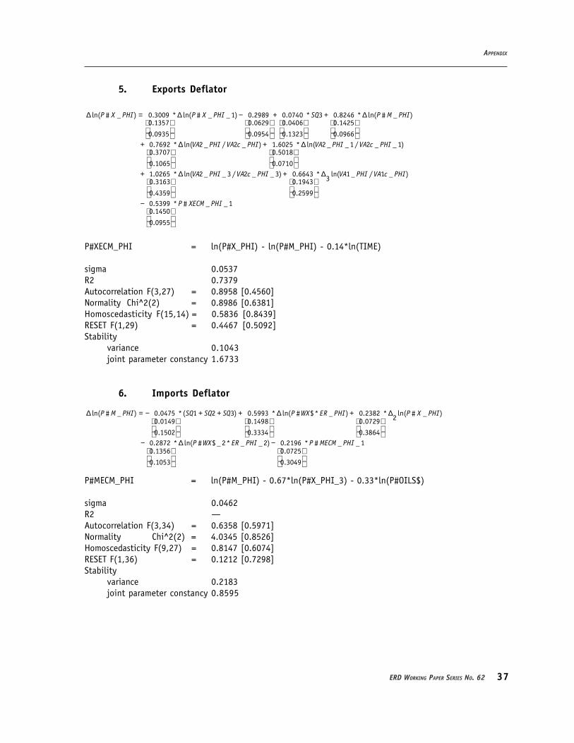
37ERD WORKING PAPER SERIES NO. 62
5. Exports Deflator
ln( # _ ) 0.3009 * ln( # _ _1) 0.2989 0.0740 * 3 0.8246 * ln( # _ )0.1357 0.0629 0.0406 0.1425
0.0935 0.0954 0.1323 0.09660.7692 * ln( 2 _ / 2 _ ) 1.60250.3707 0.
0.1065
P X PHI P X PHI SQ P M PHI
VA PHI VA c PHI
∆ = ∆ − + + ∆
+ ∆ +
* ln( 2 _ _ 1 / 2 _ _ 1)5018
0.07101.0265 * ln( 2 _ _ 3 / 2 _ _ 3) 0.6643 * ln( 1 _ / 1 _ )
30.3163 0.1943
0.4359 0.25990.5399 * # _ _10.1450
0.0955
VA PHI VA c PHI
VA PHI VA c PHI VA PHI VA c PHI
P XECM PHI
∆
+ ∆ + ∆
−
P#XECM_PHI = ln(P#X_PHI) - ln(P#M_PHI) - 0.14*ln(TIME)
sigma 0.0537R2 0.7379Autocorrelation F(3,27) = 0.8958 [0.4560]Normality Chi^2(2) = 0.8986 [0.6381]Homoscedasticity F(15,14) = 0.5836 [0.8439]RESET F(1,29) = 0.4467 [0.5092]Stability
variance 0.1043joint parameter constancy 1.6733
6. Imports Deflator
ln( # _ ) 0.0475 *( 1 2 3) 0.5993 * ln( # $* _ ) 0.2382 * ln( # _ )20.0149 0.1498 0.0729
0.1502 0.3334 0.38640.2872 * ln( # $ _ 2* _ _ 2) 0.21960.1356 0.0725
0.1053 0.3049
P M PHI SQ SQ SQ P WX ER PHI P X PHI
P WX ER PHI
∆ = − + + + ∆ + ∆
− ∆ −
* # _ _ 1P MECM PHI
P#MECM_PHI = ln(P#M_PHI) - 0.67*ln(P#X_PHI_3) - 0.33*ln(P#OILS$)
sigma 0.0462R2 —Autocorrelation F(3,34) = 0.6358 [0.5971]Normality Chi^2(2) = 4.0345 [0.8526]Homoscedasticity F(9,27) = 0.8147 [0.6074]RESET F(1,36) = 0.1212 [0.7298]Stability
variance 0.2183joint parameter constancy 0.8595
APPENDIX

38 JANUARY 2005
A SMALL MACROECONOMETRIC MODEL OF THE PHILIPPINE ECONOMY
GEOFFREY DUCANES, MARIE ANNE CAGAS, DUO QIN, PILIPINAS QUISING, AND NEDELYN MAGTIBAY-RAMOS
7. World Price of Exports
ln( # _ ) 0.1506 0.4739 ln( # _ _ 1) 0.3463 ln( # _ _ 2)20.0549 0.1662 0.1671
0.1726 0.0273 0.05010.1880 * ln( # $ _ * _ ) 0.0933 * ln( #0.0516 0.0511
0.1760 0.1145
P WX PHI P WX PH P WX PH
P OIL PHI ER PHI P O
∆ = + + ∆ + + ∆
+ ∆ − ∆
$ _ _ 2* _ _ 2)
0.0456 * 2 0.0425 * 3 0.1423 * # _ _ 10.0185 0.0189 0.0629
0.0838 0.2051 0.1905
IL PHI ER PHI
SQ SQ P WXECM PHI− − −
P#WXECM_PHI = ln(P#WXa_PHI) - 0.4065*ln(P#OILS$_2*ER_PHI_2)
sigma 0.0417R2 0.5094Autocorrelation F(3,27) = 1.5976 [0.2173]Normality Chi^2(2) = 2.5325 [0.2819]Homoscedasticity F(9,20) = 2.0188 [0.1117]RESET F(1,29) = 0.0185 [0.8928]Stability
variance 0.4055joint parameter constancy 1.2082
G. Monetary Block
1. Currency in Circulation
ln( 0 _ ) 0.1545 0.5262 * ln( 1 _ ) 0.2364 * 1 0.1879 * 2 0.1816 * 3 0.1860 * 1999 4(0.0215) (0.1253) (0.0282) (0.0194) (0.0220) (0.0299)0.1720 * 2000 1 0.2435 * 0 _ _1
(0.0316) (0.0928)
M PHI M PHI SQ SQ SQ DSH Q
DSH Q M ECM PHI
∆ = + ∆ − − − +
− −
M0ECM_PHI = ln(M0_PHI) - ln[(1 - 0.14*ln(TIME))*M1_PHI]
sigma 0.0248R2 0.9795Autocorrelation F(4,36) = 1.1831 [0.3347]Normality Chi^2(2) = 0.3897 [0.8230]Homoscedasticity F(9,30) = 0.5047 [0.8594]RESET F(1,39) = 0.0314 [0.8603]Stability: tests not performed because of impulse dummy among explanatory variables
2. Narrow Money
( )ln( 1 _ ) ln( # _ ) 0.4492 0.7888 * ln( _ ) 0.01385 * % _ 0.1518 * 199904
0.1077 0.0846 0.0054 0.0352
0.0946 0.2603 0.14190.5692 * 1 _ _10.1365
0.0945
M PHI P C PHI GNPc PHI IROB PHI DSH
M ECM PHI
∆ = ∆ − + ∆ − ∆ +
−

39ERD WORKING PAPER SERIES NO. 62
M1ECM_PHI = ln(M1_PHI/P#C_PHI) - ln(GNPc_PHI) + 0.0146*IROB%_PHI
sigma 0.0332R2 0.8872Autocorrelation F(2,17) = 2.0339 [0.1615]Normality Chi^2(2) = 2.5186 [0.2838]Homoscedasticity F(7,11) = 0.6564 [0.7040]RESET F(1,18) = 0.0454 [0.8836]Stability: tests not performed because of impulse dummy among explanatory variables
3. Broad Money
ln( 3 _ ) 0.1521 0.8655 * ln( _ _ _ ) 0.2964 * 3 _ _10.0588 0.1377 0.1125
0.2268 0.0873 0.2177
M PHI NFA PHI DCDMB PHI DCCB PHI M ECM PHI∆ = − + ∆ + + −
M3ECM_PHI = ln(M3_PHI) - ln(NFA_PHI + DCDMB_PHI + DCCB_PHI)
sigma 0.0282R2 0.5896Autocorrelation F(3,29) = 1.0146 [0.4005]Normality Chi^2(2) = 2.6285 [0.2687]Homoscedasticity F(4,27) = 1.8102 [0.1560]RESET F(1,31) = 0.0203 [0.8878]Stability
variance 0.1802joint parameter constancy 0.6234
4. Net Foreign Assets
2 _ 7460.3 8182.1 * _ _ 2 3.5674 * _ _ 2 0.5107 * ( _ _ )29888.0 3370.0 1.0020 0.1697
0.2193 0.2604 0.0942 0.10020.3288 * ( _ _ 1 _ _ 1) 0.74770.1811 0.
0.0868
NFA PHI ER PHI NFIA PHI X PHI M PHI
X PHI M PHI
∆ = + ∆ + ∆ + ∆ −
+ ∆ − −
* _ _ 11480
0.1722
NFAECM PHI
NFAECM_PHI = ∆NFA_PHI - X_PHI + M_PHI
sigma 33755.7R2 0.7628Autocorrelation F(3,22) = 1.9034 [0.1586]Normality Chi^2(2) = 5.6163 [0.0603]Homoscedasticity F(10,14) = 5.6163 [0.0603]RESET F(1,24) = 0.0202 [0.8881]Stability
variance 0.1939joint parameter constancy 1.0515
APPENDIX

40 JANUARY 2005
A SMALL MACROECONOMETRIC MODEL OF THE PHILIPPINE ECONOMY
GEOFFREY DUCANES, MARIE ANNE CAGAS, DUO QIN, PILIPINAS QUISING, AND NEDELYN MAGTIBAY-RAMOS
5. Domestic Credit of Deposit Money Banks
2 _ 60961 1.5865 * _ 8082.16 * ( % _ _ 1 _ _ 1)2 413460 0.5704 2836.0
0.1756 0.1068 0.06965847.51 * _ _ 2 1.0781 * _ _1
41943.0 0.1739
0.1197 0.2119
DCDMB PHI INV PHI IRL PHI CPI PHI
ER PHI DCDMBECM PHI
∆ = + ∆ − ∆ − ∆
− ∆ −
DCDMBECM_PHI = ∆DCDMB_PHI - INV_PHI_1 + 4862*ER_PHI_3
sigma 40218.7R2 0.6505Autocorrelation F(3,24) = 1.0349 [0.3949]Normality Chi^2(2) = 0.2924 [0.8640]Homoscedasticity F(8,18) = 0.9013 [0.5360]RESET F(1,26) = 0.0505[0.5045]Stability
variance 0.0784joint parameter constancy 0.8710
6. Domestic Credit of Central Bank
2 _ 79544.4 5308.48 * % _ _ 2 8091.30 * % _ _5 1.3638 * _ _ 19994.0 3047.0 2852.0 0.1369
0.0722 0.0897 0.1985 0.0723
DCCB PHI IRTB PHI IRTB PHI DCCBECM PHI∆ = − ∆ − ∆ −
DCCBECM_PHI = ∆DCCB_PHI - GDEF_PHI_1 + 2088*ER_PHI_1
sigma 32811.5R2 0.7697Autocorrelation F(3,29) = 1.3933 [0.2671]Normality Chi^2(2) = 0.7274 [0.6951]Homoscedasticity F(6,25) = 0.8050 [0.6270]RESET F(1,28) = 0.0002 [0.9893]Stability
variance 0.1120joint parameter constancy 0.6541

41ERD WORKING PAPER SERIES NO. 62
7. Overnight Borrowing Rate
% _ 2.7506 1.0977 * ( # _ _ 1 / # _ _ 5)*10040.9203 0.2215
0.2237 0.35220.7410 * ( # _ _2 / # _ _ 6)*100 0.7137 * % _ _ 1
40.2104 0.1459
0.2956 0.2283
IROB PHI P C PHI P C PHI
P C PHI P C PHI IRL USA
∆ = + ∆
− ∆ +
sigma 1.1100R2 0.8482Autocorrelation F(3,19) = 0.4501 [0.6446]Normality Chi^2(2) = 0.3551 [0.1694]Homoscedasticity F(8,13) = 1.0972 [0.4141]RESET F(1,21) = 7.9738 [0.0108]Stability
variance 0.2085joint parameter constancy 0.9674
8. Deposit Rate
% _ 1.2098 0.3246 * % _ 0.6492 * % _ _ 1 0.5432 * % _ _10.5739 0.0790 0.1052 0.0922
0.0308 0.2705 0.02866 0.03070.28785 * _ _ 10.0774
0.04997
IRD PHI IROB PHI IRD PHI IROB PHI
ER PHI
∆ = − + ∆ − +
+ ∆
sigma 0.7644R2 0.7386Autocorrelation F(3,19) = 2.4514 [0.0948]Normality Chi^2(2) = 0.5230 [0.7699]Homoscedasticity F(8,13) = 2.0263 [0.1240]RESET F(1,21) = 0.2017 [0.6579]Stability
variance 0.1702joint parameter constancy 0.7474
(i) Lending Rate
% _ 1.3062 0.3031 * % _ _ 1 0.2194 * % _ _ 1 8.0652 * ln( _ )0.7300 0.0829 0.0919 4.4860
0.1416 0.1422 0.1633 0.30360.3621 * % _ 0.19720.1355 0.1061
0.3587 0.2607
IRL PHI IRL PHI IROB PHI ER PHI
IRTB PHI
∆ = − + + ∆
+ ∆ +
* % _ _1IRTB PHI∆
IRL%ECM_PHI = IRL%_PHI - 0.8*IRTB%_PHI
sigma 0.8639R2 0.7614Autocorrelation F(3,18) = 0.5168 [0.6760]
APPENDIX
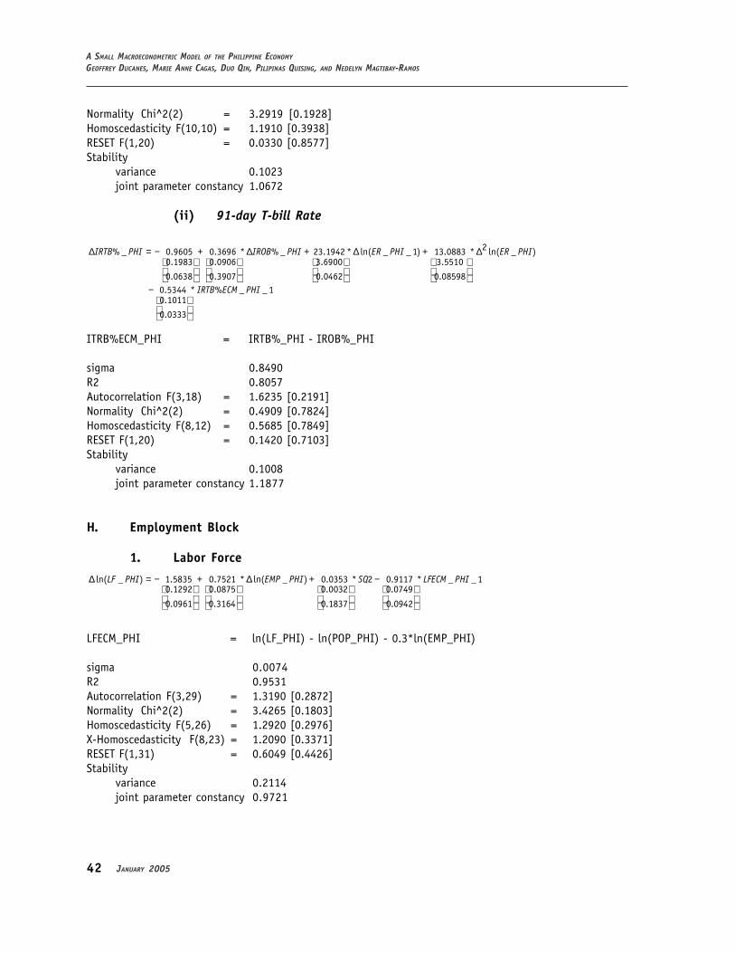
42 JANUARY 2005
A SMALL MACROECONOMETRIC MODEL OF THE PHILIPPINE ECONOMY
GEOFFREY DUCANES, MARIE ANNE CAGAS, DUO QIN, PILIPINAS QUISING, AND NEDELYN MAGTIBAY-RAMOS
Normality Chi^2(2) = 3.2919 [0.1928]Homoscedasticity F(10,10) = 1.1910 [0.3938]RESET F(1,20) = 0.0330 [0.8577]Stability
variance 0.1023joint parameter constancy 1.0672
(ii) 91-day T-bill Rate
2% _ 0.9605 0.3696 * % _ 23.1942 * ln( _ _ 1) 13.0883 * ln( _ )0.1983 0.0906 3.6900 3.5510
0.0638 0.3907 0.0462 0.085980.5344 * % _ _ 10.1011
0.0333
IRTB PHI IROB PHI ER PHI ER PHI
IRTB ECM PHI
∆ = − + ∆ + ∆ + ∆
−
ITRB%ECM_PHI = IRTB%_PHI - IROB%_PHI
sigma 0.8490R2 0.8057Autocorrelation F(3,18) = 1.6235 [0.2191]Normality Chi^2(2) = 0.4909 [0.7824]Homoscedasticity F(8,12) = 0.5685 [0.7849]RESET F(1,20) = 0.1420 [0.7103]Stability
variance 0.1008joint parameter constancy 1.1877
H. Employment Block
1. Labor Force
ln( _ ) 1.5835 0.7521 * ln( _ ) 0.0353 * 2 0.9117 * _ _10.1292 0.0875 0.0032 0.0749
0.0961 0.3164 0.1837 0.0942
LF PHI EMP PHI SQ LFECM PHI∆ = − + ∆ + −
LFECM_PHI = ln(LF_PHI) - ln(POP_PHI) - 0.3*ln(EMP_PHI)
sigma 0.0074R2 0.9531Autocorrelation F(3,29) = 1.3190 [0.2872]Normality Chi^2(2) = 3.4265 [0.1803]Homoscedasticity F(5,26) = 1.2920 [0.2976]X-Homoscedasticity F(8,23) = 1.2090 [0.3371]RESET F(1,31) = 0.6049 [0.4426]Stability
variance 0.2114joint parameter constancy 0.9721

43ERD WORKING PAPER SERIES NO. 62
2. Total Employed
ln( _ ) 0.2837 0.1661 * ln( 1 _ ) 1.2169 * ( 1 _ _ 1 / _ _1)30.03835 0.0203 0.1928
0.18215 0.2027 0.40630.7745 * ( 3 _ _1 / _ _ 1) 0.2886
30.2398 0.0378
0.3120 0.1736
EMP PHI VA c PHI VA c PHI GDPc PHI
VA c PHI GDPc PHI
∆ = − + ∆ + ∆
+ ∆ −
* _ _ 1EMPECM PHI
EMPECM_PHI = ln(EMP_PHI) - 0.26*ln(VA1c_PHI) - 0.37*ln(VA2c_PHI_2) -0.37*ln(VA3c_PHI_1) + 0.13*ln(WAGE_PHI_2/P#GDP_PHI_2) -2.2*(VA1c_PHI_3/GDPc_PHI_3)
sigma 0.0095R2 0.7187Autocorrelation F(3,32) = 0.1771 [0.9111]Normality Chi^2(2) = 2.7159 [0.2572]Homoscedasticity F(8,26) = 2.2639 [0.0551]RESET F(1,34) = 0.0337 [0.8555]Stability
variance 0.2484joint parameter constancy 1.2865
3. Employed in the Tertiary Sector3 _ 2_ exp[ln( 2 _ 3_ ) 0.3120 0.0320 * 1998 3 0.1240 * 3 _ _1]
(0.0701) (0.0118) (0.0268)EMP PHI EMP PHI EMP PHI EMP PHI DSH Q EMP ECM PHI= − + + − − −
EMP3ECM_PHI = ln(EMP3_PHI+EMP2_PHI) - ln(VA2c_PHI_1 + VA3c_PHI_1) +0.06*[ln(WAGE_PHI_1) - ln (P#GDP_PHI_1)]
sigma 0.0114R2 0.4931Autocorrelation F(3,34) = 1.8257 [0.1611]Normality Chi^2(2) = 5.0232 [0.0811]Homoscedasticity F(3,33) = 0.6663 [0.5788]RESET F(1,36) = 0.0593 [0.8089]Stability: tests not performed because of impulse dummy among explanatory variables
4. Employed in the Secondary Sector
ln( 2 _ ) 0.161996 0.0797 * ln( 2 _ ) 1.0152 * ( 1 _ / _ )0.0199 0.0272 0.2642
0.2169 0.0896 0.09990.1730 * ln( 2 _ / 2 _ ) 0.0
20.0683
0.1138
EMP PHI VA c PHI EMP PHI EMP PHI
VA PHI VA c PHI
∆ = + ∆ − ∆
− ∆ − 145 * ln( _ ) 0.4613 * 2 _ _ 130.0068 0.0553
0.0714 0.1763
WAGE PHI EMP ECM PHI
∆ −
EMP2ECM_PHI = ln(EMP2_PHI) - 0.64*ln(VA2c_PHI_1) - 0.4*ln(WAGE_PHI)sigma 0.0168R2 0.7193
APPENDIX

44 JANUARY 2005
A SMALL MACROECONOMETRIC MODEL OF THE PHILIPPINE ECONOMY
GEOFFREY DUCANES, MARIE ANNE CAGAS, DUO QIN, PILIPINAS QUISING, AND NEDELYN MAGTIBAY-RAMOS
Autocorrelation F(4,38) = 0.3088 [0.8703]Normality Chi^2(2) = 6.8307 [0.0329]*Homoscedasticity F(10,31) = 0.6155 [0.7888]RESET F(1,41) = 1.3625 [0.2498]Stability
variance 0.0664joint parameter constancy 0.8788
I. Identities
1. Investment Block
INV_PHI = INVc_PHI*P#INV_PHI
K_PHI = K_PHI(-1)*[1 - DEPK%_PHI/400] + INV_PHI
Kc_PHI = K_PHI/P#INV_PHI
UCC%_PHI = [IRL%_PHI/4 - 100*([P#INV_PHI + P#INV_PHI(-1) + P#INV_PHI(-2) + P#INV_PHI(-3)] / [P#INV_PHI(-1) + P#INV_PHI(-2) + P#INV_PHI(-3) + P#INV_PHI(-4)] -1 ) + DEPK%_PHI/4] * [0.25*(P#INV_PHI +P#INV_PHI(-1) + P#INV_PHI(-2) + P#INV_PHI(-3))] / P#GDP_PHI / (1 - TAX%_PHI/100)
2. Government Block
GEXP_PHI = GPAY_PHI + GINT_PHI
GDEF_PHI = GREV_PHI - GEXP_PHI
TDEBTr_PHI = (DDEBT_PHI_1*SQ1 + DDEBT_PHI_2*SQ2 + DDEBT_PHI_3*SQ3 + DDEBT_PHI_4*SQ4 +FDEBT_PHI_1*SQ1 + FDEBT_PHI_2*SQ2 + FDEBT_PHI_3*SQ3 + FDEBT_PHI_4*SQ4) / [(GDP_PHI_1 +GDP_PHI_2 + GDP_PHI_3 + GDP_PHI_4)*SQ1 + (GDP_PHI_2 + GDP_PHI_3 + GDP_PHI_4 +GDP_PHI_5)*SQ2 + (GDP_PHI_3 + GDP_PHI_4 + GDP_PHI_5 + GDP_PHI_6)*SQ3 + (GDP_PHI_4 +GDP_PHI_5 + GDP_PHI_6 + GDP_PHI_7)*SQ4]
GDEFr_PHI = [(GDEF_PHI_1 + GDEF_PHI_2 + GDEF_PHI_3 + GDEF_PHI_4)*SQ1 + (GDEF_PHI_2 + GDEF_PHI_3 +GDEF_PHI_4 + GDEF_PHI_5)*SQ2 + (GDEF_PHI_3 + GDEF_PHI_4 + GDEF_PHI_5 + GDEF_PHI_6)*SQ3 +(GDEF_PHI_4 + GDEF_PHI_5 + GDEF_PHI_6 + GDEF_PHI_7)*SQ4] / [(GDP_PHI_1 + GDP_PHI_2 +GDP_PHI_3 + GDP_PHI_4)*SQ1 + (GDP_PHI_2 + GDP_PHI_3 + GDP_PHI_4 + GDP_PHI_5)*SQ2 +(GDP_PHI_3 + GDP_PHI_4 + GDP_PHI_5 + GDP_PHI_6)*SQ3 + (GDP_PHI_4 + GDP_PHI_5 + GDP_PHI_6+ GDP_PHI_7)*SQ4]
TEFT%_PHI = 100*[(GTAX_PHI_1 + GTAX_PHI_2 + GTAX_PHI_3 + GTAX_PHI_4)*SQ1 + (GTAX_PHI_2 + GTAX_PHI_3+ GTAX_PHI_4 + GTAX_PHI_5)*SQ2 + (GTAX_PHI_3 + GTAX_PHI_4 + GTAX_PHI_5 + GTAX_PHI_6)*SQ3 +(GTAX_PHI_4 + GTAX_PHI_5 + GTAX_PHI_6 + GTAX_PHI_7)*SQ4] / [(GDP_PHI_1 + GDP_PHI_2 +GDP_PHI_3 + GDP_PHI_4)*SQ1 + (GDP_PHI_2 + GDP_PHI_3 + GDP_PHI_4 + GDP_PHI_5)*SQ2 +(GDP_PHI_3 + GDP_PHI_4 + GDP_PHI_5 + GDP_PHI_6)*SQ3 + (GDP_PHI_4 + GDP_PHI_5 + GDP_PHI_6+ GDP_PHI_7)*SQ4]
BEFT%_PHI = DST90Q104Q1*TEFT%_PHI + DST2004Q1*BEFT%_PHI_1

45ERD WORKING PAPER SERIES NO. 62
3. Trade Block
X_PHI = X$_PHI * ER_PHI
Xc_PHI = X_PHI / P#X_PHI
Mc_PHI = M_PHI / P#M_PHI
M$_PHI = M_PHI / ER_PHI
4. Production Block
GDPc_PHI = VA1c_PHI + VA2c_PHI + VA3c_PHI
GDP_PHI = GDPc_PHI*P#GDP_PHI
GNP_PHI = GDP_PHI + NFIA_PHI
NFIAc_PHI = GNPc_PHI - GDPc_PHI
5. Price Block
P#INV_PHI(-2) + P#INV_PHI(-3) + P#INV_PHI(-4)] -1 ) + DEPK%_PHI/4] * [0.25*(P#INV_PHI + P#INV_PHI(-1) + P#INV_PHI(-2) + P#INV_PHI(-3))] / P#GDP_PHI / (1 - TAX%_PHI/100)
P#P$_PHI = P#P_PHI/ER_PHI
WAGE_PHI = [GDP_PHI - UCC%_PHI*K_PHI/100] / (EMP_PHI/1000)
P#WX$ = DST90Q104Q2*P#WX$ + DST2004Q2*P#Wxa_PHI/ER_PHI
6. Monetary Block
MQ_PHI = M3_PHI - M1_PHI
7. Employment Block
UEMP%_PHI = (LF_PHI - EMP_PHI) / LF_PHI *100EMP1_PHI = EMP_PHI - EMP2_PHI - EMP3_PHI
APPENDIX
46 JANUARY 2005
A SMALL MACROECONOMETRIC MODEL OF THE PHILIPPINE ECONOMY
GEOFFREY DUCANES, MARIE ANNE CAGAS, DUO QIN, PILIPINAS QUISING, AND NEDELYN MAGTIBAY-RAMOS
REFERENCES
Bautista, C. C., R. S. Mariano, and B. V. Bawagan, 2004. “The NEDA Quarterly Macroeconomic Model: TheoreticalStructure and Some Empirical results.” Paper presented during the 9th National Convention in Statistics,October, Manila, Philippines.
Doornik, J. A., and D. F. Hendry, 2001. Empircal Econometric Modelling Using PcGive. London: Timberlake ConsultantsLtd.
Engle, R. F., D. F. Hendry, and J. F. Richard, 1983. “Exogeneity.” Econometrica 51:277-304.Favero, C., and F. Giavazzi, 2003. “Monetary Policy when Debt and Default Risk are High: Lessons from Brazil.”
Processed. Available: http://cep.lse.ac.uk/seminarpapers/22-05-03-GIA.pdf.Gochoco-Bautista, M. S., and D. Canlas, 2003. “Monetary and Exchange Rate Policy.” In A. Balisacan and H.
Hill, eds., The Philippine Economy: Development, Policies, and Challenges. Manila: Ateneo de Manila UniversityPress.
He, X. H., D. Qin, and P. Quising, 2004. “Macroeconomic Model of China: Summary Report.” Economics andResearch Department, Asian Development Bank. Processed.
Hendry, D. F., 1995. Dynamic Economics. Oxford: Oxford University Press. , 2002. “Applied Econometrics without Sinning.” Journal of Economic Surveys 16:591-604.
Hendry, D. F., and H-M. Krolzig, 2001. Automatic Econometric Model Selection Using PcGets. London: TimberlakeConsultants Ltd.
Hill, H., 2003. “Industry.” In A. Balisacan and H. Hill, eds. The Philippine Economy: Development, Policies,and Challenges. Manila: Ateneo de Manila University Press.
Lucas, R. E., 1976. “Econometric Policy Evaluation: A Critique.” In K. Brunner and A. Meltzer, eds., The PhillipsCurve and Labor Markets, Vol. 1, Cornegie-Rochester Conferences on Public Policy. Amsterdam: North-HollandPublishing Company.
Pagan, A., 1999. “The Getting of Macroeconomic Wisdom.” Paper delivered during the 12th World Congress ofthe International Economic Association, August, Buenos Aires, Argentina.
, 2003. “An Examination of Some Tools for Macro-econometric Model Building.” METU Lecture at ERCConference VII, September, Ankara.
Pierse, R., 2001. Winsolve Manual. Department of Economics, University of Surrey, United Kingdom.Sicat, G., and R. Abdula, 2003. “Public Finance.” In A. Balisacan and H. Hill, eds. The Philippine Economy:
Development, Policies, and Challenges. Manila: Ateneo de Manila University Press.Taylor, J. B., 1993. “Discretion versus Policy Rules in Practice.” Carnegie-Rochester Conference Series on Public
Policy 39:195-214.Yap, J. T., 2000. PIDS Annual Macroeconometric Model 2000. Discussion Paper Series 2000-13, Philippine
Institute for Development Studies, Makati City, Philippines. , 2002. A Perspective on Macroeconomic and Economy-wide Quantitative Models of the Philippines: 1990-
2002. Philippine Institute for Development Studies, Manila.

47
PUBLICATIONS FROM THEECONOMICS AND RESEARCH DEPARTMENT
ERD WORKING PAPER SERIES (WPS)(Published in-house; Available through ADB Office of External Relations; Free of Charge)
No. 1 Capitalizing on Globalization—Barry Eichengreen, January 2002
No. 2 Policy-based Lending and Poverty Reduction:An Overview of Processes, Assessmentand Options—Richard Bolt and Manabu Fujimura
January 2002No. 3 The Automotive Supply Chain: Global Trends
and Asian Perspectives—Francisco Veloso and Rajiv Kumar
January 2002No. 4 International Competitiveness of Asian Firms:
An Analytical Framework—Rajiv Kumar and Doren Chadee
February 2002No. 5 The International Competitiveness of Asian
Economies in the Apparel Commodity Chain—Gary Gereffi
February 2002No. 6 Monetary and Financial Cooperation in East
Asia—The Chiang Mai Initiative and Beyond—Pradumna B. Rana
February 2002No. 7 Probing Beneath Cross-national Averages: Poverty,
Inequality, and Growth in the Philippines—Arsenio M. Balisacan and Ernesto M. Pernia
March 2002No. 8 Poverty, Growth, and Inequality in Thailand
—Anil B. DeolalikarApril 2002
No. 9 Microfinance in Northeast Thailand: Who Benefitsand How Much?—Brett E. Coleman
April 2002No. 10 Poverty Reduction and the Role of Institutions in
Developing Asia—Anil B. Deolalikar, Alex B. Brilliantes, Jr.,
Raghav Gaiha, Ernesto M. Pernia, Mary Raceliswith the assistance of Marita Concepcion Castro-Guevara, Liza L. Lim, Pilipinas F. QuisingMay 2002
No. 11 The European Social Model: Lessons forDeveloping Countries—Assar Lindbeck
May 2002No. 12 Costs and Benefits of a Common Currency for
ASEAN—Srinivasa Madhur
May 2002No. 13 Monetary Cooperation in East Asia: A Survey
—Raul FabellaMay 2002
No. 14 Toward A Political Economy Approachto Policy-based Lending—George Abonyi
May 2002No. 15 A Framework for Establishing Priorities in a
Country Poverty Reduction Strategy—Ron Duncan and Steve Pollard
June 2002
No. 16 The Role of Infrastructure in Land-use Dynamicsand Rice Production in Viet Nam’s Mekong RiverDelta—Christopher Edmonds
July 2002No. 17 Effect of Decentralization Strategy on
Macroeconomic Stability in Thailand—Kanokpan Lao-Araya
August 2002No. 18 Poverty and Patterns of Growth
—Rana Hasan and M. G. QuibriaAugust 2002
No. 19 Why are Some Countries Richer than Others?A Reassessment of Mankiw-Romer-Weil’s Test ofthe Neoclassical Growth Model—Jesus Felipe and John McCombie
August 2002No. 20 Modernization and Son Preference in People’s
Republic of China—Robin Burgess and Juzhong Zhuang
September 2002No. 21 The Doha Agenda and Development: A View from
the Uruguay Round—J. Michael Finger
September 2002No. 22 Conceptual Issues in the Role of Education
Decentralization in Promoting Effective Schooling inAsian Developing Countries—Jere R. Behrman, Anil B. Deolalikar, and Lee-
Ying SonSeptember 2002
No. 23 Promoting Effective Schooling through EducationDecentralization in Bangladesh, Indonesia, andPhilippines—Jere R. Behrman, Anil B. Deolalikar, and Lee- Ying Son
September 2002No. 24 Financial Opening under the WTO Agreement in
Selected Asian Countries: Progress and Issues—Yun-Hwan Kim
September 2002No. 25 Revisiting Growth and Poverty Reduction in
Indonesia: What Do Subnational Data Show?—Arsenio M. Balisacan, Ernesto M. Pernia, and Abuzar Asra October 2002
No. 26 Causes of the 1997 Asian Financial Crisis: WhatCan an Early Warning System Model Tell Us?—Juzhong Zhuang and J. Malcolm Dowling October 2002
No. 27 Digital Divide: Determinants and Policies withSpecial Reference to Asia—M. G. Quibria, Shamsun N. Ahmed, TedTschang, and Mari-Len Reyes-Macasaquit October 2002
No. 28 Regional Cooperation in Asia: Long-term Progress,Recent Retrogression, and the Way Forward—Ramgopal Agarwala and Brahm Prakash
October 2002

48
No. 29 How can Cambodia, Lao PDR, Myanmar, and VietNam Cope with Revenue Lost Due to AFTA TariffReductions?—Kanokpan Lao-Araya
November 2002No. 30 Asian Regionalism and Its Effects on Trade in the
1980s and 1990s—Ramon Clarete, Christopher Edmonds, andJessica Seddon Wallack
November 2002No. 31 New Economy and the Effects of Industrial
Structures on International Equity MarketCorrelations—Cyn-Young Park and Jaejoon Woo
December 2002No. 32 Leading Indicators of Business Cycles in Malaysia
and the Philippines—Wenda Zhang and Juzhong Zhuang
December 2002No. 33 Technological Spillovers from Foreign Direct
Investment—A Survey—Emma Xiaoqin Fan
December 2002No. 34 Economic Openness and Regional Development in
the Philippines—Ernesto M. Pernia and Pilipinas F. Quising
January 2003No. 35 Bond Market Development in East Asia:
Issues and Challenges—Raul Fabella and Srinivasa Madhur
January 2003No. 36 Environment Statistics in Central Asia: Progress
and Prospects—Robert Ballance and Bishnu D. Pant
March 2003No. 37 Electricity Demand in the People’s Republic of
China: Investment Requirement andEnvironmental Impact—Bo Q. Lin
March 2003No. 38 Foreign Direct Investment in Developing Asia:
Trends, Effects, and Likely Issues for theForthcoming WTO Negotiations—Douglas H. Brooks, Emma Xiaoqin Fan,and Lea R. Sumulong
April 2003No. 39 The Political Economy of Good Governance for
Poverty Alleviation Policies—Narayan Lakshman
April 2003No. 40 The Puzzle of Social Capital
A Critical Review—M. G. Quibria
May 2003No. 41 Industrial Structure, Technical Change, and the
Role of Government in Development of theElectronics and Information Industry inTaipei,China—Yeo Lin
May 2003No. 42 Economic Growth and Poverty Reduction
in Viet Nam—Arsenio M. Balisacan, Ernesto M. Pernia, andGemma Esther B. Estrada
June 2003No. 43 Why Has Income Inequality in Thailand
Increased? An Analysis Using 1975-1998 Surveys—Taizo Motonishi
June 2003
No. 44 Welfare Impacts of Electricity Generation SectorReform in the Philippines—Natsuko Toba
June 2003No. 45 A Review of Commitment Savings Products in
Developing Countries—Nava Ashraf, Nathalie Gons, Dean S. Karlan,and Wesley Yin
July 2003No. 46 Local Government Finance, Private Resources,
and Local Credit Markets in Asia—Roberto de Vera and Yun-Hwan Kim
October 2003July 2003
No. 47 Excess Investment and Efficiency Loss DuringReforms: The Case of Provincial-level Fixed-AssetInvestment in People’s Republic of China—Duo Qin and Haiyan Song
October 2003No. 48 Is Export-led Growth Passe? Implications for
Developing Asia—Jesus Felipe
December 2003No. 49 Changing Bank Lending Behavior and Corporate
Financing in Asia—Some Research Issues—Emma Xiaoqin Fan and Akiko Terada-Hagiwara
December 2003No. 50 Is People’s Republic of China’s Rising Services
Sector Leading to Cost Disease?—Duo Qin
March 2004No. 51 Poverty Estimates in India: Some Key Issues
—Savita SharmaMay 2004
No. 52 Restructuring and Regulatory Reform in the PowerSector: Review of Experience and Issues—Peter Choynowski
May 2004No. 53 Competitiveness, Income Distribution, and Growth
in the Philippines: What Does the Long-runEvidence Show?—Jesus Felipe and Grace C. Sipin
June 2004No. 54 Practices of Poverty Measurement and Poverty
Profile of Bangladesh—Faizuddin Ahmed
August 2004No. 55 Experience of Asian Asset Management
Companies: Do They Increase Moral Hazard?—Evidence from Thailand—Akiko Terada-Hagiwara and Gloria Pasadilla
September 2004No. 56 Viet Nam: Foreign Direct Investment and
Postcrisis Regional Integration—Vittorio Leproux and Douglas H. Brooks
September 2004No. 57 Practices of Poverty Measurement and Poverty
Profile of Nepal—Devendra Chhetry
September 2004No. 58 Monetary Poverty Estimates in Sri Lanka:
Selected Issues—Neranjana Gunetilleke and Dinushka Senanayake
October 2004No. 59 Labor Market Distortions, Rural-Urban Inequality,
and the Opening of People’s Republic of China’sEconomy—Thomas Hertel and Fan Zhai
November 2004

49
—Erik Bloom and Peter ChoynowskiMay 2003
No. 7 Strengthening the Economic Analysis of NaturalResource Management Projects—Keith Ward
September 2003No. 8 Testing Savings Product Innovations Using an
Experimental Methodology—Nava Ashraf, Dean S. Karlan, and Wesley Yin
November 2003No. 9 Setting User Charges for Public Services: Policies
and Practice at the Asian Development Bank—David Dole
December 2003No. 10 Beyond Cost Recovery: Setting User Charges for
Financial, Economic, and Social Goals—David Dole and Ian Bartlett
January 2004No. 11 Shadow Exchange Rates for Project Economic
Analysis: Toward Improving Practice at the AsianDevelopment Bank—Anneli Lagman-Martin
February 2004
ERD POLICY BRIEF SERIES (PBS)(Published in-house; Available through ADB Office of External Relations; Free of charge)
No. 1 Is Growth Good Enough for the Poor?—Ernesto M. Pernia, October 2001
No. 2 India’s Economic ReformsWhat Has Been Accomplished?What Remains to Be Done?—Arvind Panagariya, November 2001
No. 3 Unequal Benefits of Growth in Viet Nam—Indu Bhushan, Erik Bloom, and Nguyen MinhThang, January 2002
No. 4 Is Volatility Built into Today’s World Economy?—J. Malcolm Dowling and J.P. Verbiest,February 2002
No. 5 What Else Besides Growth Matters to PovertyReduction? Philippines—Arsenio M. Balisacan and Ernesto M. Pernia,February 2002
ERD TECHNICAL NOTE SERIES (TNS)(Published in-house; Available through ADB Office of External Relations; Free of Charge)
No. 1 Contingency Calculations for EnvironmentalImpacts with Unknown Monetary Values—David Dole February 2002
No. 2 Integrating Risk into ADB’s Economic Analysisof Projects—Nigel Rayner, Anneli Lagman-Martin,
and Keith Ward June 2002
No. 3 Measuring Willingness to Pay for Electricity—Peter Choynowski July 2002
No. 4 Economic Issues in the Design and Analysis of aWastewater Treatment Project—David Dole
July 2002No. 5 An Analysis and Case Study of the Role of
Environmental Economics at the AsianDevelopment Bank—David Dole and Piya Abeygunawardena
September 2002No. 6 Economic Analysis of Health Projects: A Case Study
in Cambodia
No. 6 Achieving the Twin Objectives of Efficiency andEquity: Contracting Health Services in Cambodia—Indu Bhushan, Sheryl Keller, and Brad Schwartz,March 2002
No. 7 Causes of the 1997 Asian Financial Crisis: WhatCan an Early Warning System Model Tell Us?—Juzhong Zhuang and Malcolm Dowling,June 2002
No. 8 The Role of Preferential Trading Arrangementsin Asia—Christopher Edmonds and Jean-Pierre Verbiest,July 2002
No. 9 The Doha Round: A Development Perspective—Jean-Pierre Verbiest, Jeffrey Liang, and LeaSumulong
July 2002
No. 60 Measuring Competitiveness in the World’s SmallestEconomies: Introducing the SSMECI—Ganeshan Wignaraja and David Joiner
November 2004No. 61 Foreign Exchange Reserves, Exchange Rate
Regimes, and Monetary Policy: Issues in Asia—Akiko Terada-Hagiwara
January 2005No. 62 A Small Macroeconometric Model of the Philippine
Economy—Geoffrey Ducanes, Marie Anne Cagas, Duo Qin, Pilipinas Quising, and Nedelyn Magtibay-Ramos
January 2005

50
SERIALS(Co-published with Oxford University Press; Available commercially through Oxford University PressOffices, Associated Companies, and Agents)
1. Asian Development Outlook (ADO; annual)$36.00 (paperback)
2. Key Indicators of Developing Asian and Pacific Countries (KI; annual)$35.00 (paperback)
JOURNAL(Published in-house; Available commercially through ADB Office of External Relations)
1. Asian Development Review (ADR; semiannual)$5.00 per issue; $8.00 per year (2 issues)
No. 10 Is Economic Openness Good for RegionalDevelopment and Poverty Reduction? ThePhilippines—E. M. Pernia and P. F. Quising
October 2002No. 11 Implications of a US Dollar Depreciation for Asian
Developing Countries—Emma Fan
July 2002No. 12 Dangers of Deflation
—D. Brooks and P. F. QuisingDecember 2002
No. 13 Infrastructure and Poverty Reduction—What is the Connection?—I. Ali and E. Pernia
January 2003No. 14 Infrastructure and Poverty Reduction—
Making Markets Work for the Poor—Xianbin Yao
May 2003No. 15 SARS: Economic Impacts and Implications
—Emma Xiaoqin FanMay 2003
No. 16 Emerging Tax Issues: Implications of Globalizationand Technology—Kanokpan Lao Araya
May 2003No. 17 Pro-Poor Growth: What is It and Why is It
Important?—Ernesto M. Pernia
May 2003No. 18 Public–Private Partnership for Competitiveness
—Jesus FelipeJune 2003
No. 19 Reviving Asian Economic Growth Requires FurtherReforms—Ifzal Ali
June 2003No. 20 The Millennium Development Goals and Poverty:
Are We Counting the World’s Poor Right?—M. G. Quibria
July 2003No. 21 Trade and Poverty: What are the Connections?
—Douglas H. BrooksJuly 2003
No. 22 Adapting Education to the Global Economy—Olivier Dupriez September 2003
No. 23 Avian Flu: An Economic Assessment for SelectedDeveloping Countries in Asia—Jean-Pierre Verbiest and Charissa Castillo March 2004
No. 25 Purchasing Power Parities and the InternationalComparison Program in a Globalized World—Bishnu Pant March 2004
No. 26 A Note on Dual/Multiple Exchange Rates—Emma Xiaoqin Fan May 2004
No. 27 Inclusive Growth for Sustainable Poverty Reductionin Developing Asia: The Enabling Role ofInfrastructure Development—Ifzal Ali and Xianbin Yao May 2004
No. 28 Higher Oil Prices: Asian Perspectives andImplications for 2004-2005—Cyn-Young Park June 2004
No. 29 Accelerating Agriculture and Rural Development forInclusive Growth: Policy Implications forDeveloping Asia—Richard Bolt July 2004
No. 30 Living with Higher Interest Rates: Is Asia Ready?—Cyn-Young Park August 2004
No. 31 Reserve Accumulation, Sterilization, and PolicyDilemma—Akiko Terada-Hagiwara October 2004
32 The Primacy of Reforms in the Emergence ofPeople’s Republic of China and India—Ifzal Ali and Emma Xiaoqin Fan November 2004
33 Population Health and Foreign Direct Investment:Does Poor Health Signal Poor GovernmentEffectiveness?—Ajay Tandon January 2005

51
MONOGRAPH SERIES(Published in-house; Available through ADB Office of External Relations; Free of charge)
EDRC REPORT SERIES (ER)
No. 1 ASEAN and the Asian Development Bank—Seiji Naya, April 1982
No. 2 Development Issues for the Developing Eastand Southeast Asian Countriesand International Cooperation—Seiji Naya and Graham Abbott, April 1982
No. 3 Aid, Savings, and Growth in the Asian Region—J. Malcolm Dowling and Ulrich Hiemenz,
April 1982No. 4 Development-oriented Foreign Investment
and the Role of ADB—Kiyoshi Kojima, April 1982
No. 5 The Multilateral Development Banksand the International Economy’s MissingPublic Sector—John Lewis, June 1982
No. 6 Notes on External Debt of DMCs—Evelyn Go, July 1982
No. 7 Grant Element in Bank Loans—Dal Hyun Kim, July 1982
No. 8 Shadow Exchange Rates and StandardConversion Factors in Project Evaluation—Peter Warr, September 1982
No. 9 Small and Medium-Scale ManufacturingEstablishments in ASEAN Countries:Perspectives and Policy Issues—Mathias Bruch and Ulrich Hiemenz,
January 1983No. 10 A Note on the Third Ministerial Meeting of GATT
—Jungsoo Lee, January 1983No. 11 Macroeconomic Forecasts for the Republic
of China, Hong Kong, and Republic of Korea—J.M. Dowling, January 1983
No. 12 ASEAN: Economic Situation and Prospects—Seiji Naya, March 1983
No. 13 The Future Prospects for the DevelopingCountries of Asia—Seiji Naya, March 1983
No. 14 Energy and Structural Change in the Asia-Pacific Region, Summary of the ThirteenthPacific Trade and Development Conference—Seiji Naya, March 1983
No. 15 A Survey of Empirical Studies on Demandfor Electricity with Special Emphasis on PriceElasticity of Demand—Wisarn Pupphavesa, June 1983
No. 16 Determinants of Paddy Production in Indonesia:1972-1981–A Simultaneous Equation ModelApproach—T.K. Jayaraman, June 1983
No. 17 The Philippine Economy: EconomicForecasts for 1983 and 1984—J.M. Dowling, E. Go, and C.N. Castillo,
June 1983No. 18 Economic Forecast for Indonesia
—J.M. Dowling, H.Y. Kim, Y.K. Wang,and C.N. Castillo, June 1983
No. 19 Relative External Debt Situation of AsianDeveloping Countries: An Applicationof Ranking Method—Jungsoo Lee, June 1983
No. 20 New Evidence on Yields, Fertilizer Application,and Prices in Asian Rice Production—William James and Teresita Ramirez, July 1983
No. 21 Inflationary Effects of Exchange RateChanges in Nine Asian LDCs—Pradumna B. Rana and J. Malcolm Dowling, Jr., December 1983
No. 22 Effects of External Shocks on the Balanceof Payments, Policy Responses, and DebtProblems of Asian Developing Countries—Seiji Naya, December 1983
No. 23 Changing Trade Patterns and Policy Issues:The Prospects for East and Southeast AsianDeveloping Countries—Seiji Naya and Ulrich Hiemenz, February 1984
No. 24 Small-Scale Industries in Asian EconomicDevelopment: Problems and Prospects—Seiji Naya, February 1984
No. 25 A Study on the External Debt IndicatorsApplying Logit Analysis—Jungsoo Lee and Clarita Barretto, February 1984
No. 26 Alternatives to Institutional Credit Programsin the Agricultural Sector of Low-IncomeCountries—Jennifer Sour, March 1984
No. 27 Economic Scene in Asia and Its Special Features—Kedar N. Kohli, November 1984
No. 28 The Effect of Terms of Trade Changes on theBalance of Payments and Real NationalIncome of Asian Developing Countries—Jungsoo Lee and Lutgarda Labios, January 1985
No. 29 Cause and Effect in the World Sugar Market:Some Empirical Findings 1951-1982—Yoshihiro Iwasaki, February 1985
No. 30 Sources of Balance of Payments Problemin the 1970s: The Asian Experience—Pradumna Rana, February 1985
No. 31 India’s Manufactured Exports: An Analysisof Supply Sectors—Ifzal Ali, February 1985
No. 32 Meeting Basic Human Needs in AsianDeveloping Countries—Jungsoo Lee and Emma Banaria, March 1985
No. 33 The Impact of Foreign Capital Inflowon Investment and Economic Growthin Developing Asia—Evelyn Go, May 1985
No. 34 The Climate for Energy Developmentin the Pacific and Asian Region:Priorities and Perspectives—V.V. Desai, April 1986
No. 35 Impact of Appreciation of the Yen onDeveloping Member Countries of the Bank—Jungsoo Lee, Pradumna Rana, and Ifzal Ali,
May 1986No. 36 Smuggling and Domestic Economic Policies
in Developing Countries—A.H.M.N. Chowdhury, October 1986
No. 37 Public Investment Criteria: Economic InternalRate of Return and Equalizing Discount Rate—Ifzal Ali, November 1986
No. 38 Review of the Theory of Neoclassical PoliticalEconomy: An Application to Trade Policies—M.G. Quibria, December 1986
No. 39 Factors Influencing the Choice of Location:Local and Foreign Firms in the Philippines—E.M. Pernia and A.N. Herrin, February 1987
No. 40 A Demographic Perspective on DevelopingAsia and Its Relevance to the Bank—E.M. Pernia, May 1987
No. 41 Emerging Issues in Asia and Social CostBenefit Analysis—I. Ali, September 1988
No. 42 Shifting Revealed Comparative Advantage:

52
No. 1 International Reserves:Factors Determining Needs and Adequacy—Evelyn Go, May 1981
No. 2 Domestic Savings in Selected DevelopingAsian Countries—Basil Moore, assisted by
A.H.M. Nuruddin Chowdhury, September 1981No. 3 Changes in Consumption, Imports and Exports
of Oil Since 1973: A Preliminary Survey ofthe Developing Member Countriesof the Asian Development Bank—Dal Hyun Kim and Graham Abbott,
September 1981No. 4 By-Passed Areas, Regional Inequalities,
and Development Policies in SelectedSoutheast Asian Countries—William James, October 1981
No. 5 Asian Agriculture and Economic Development—William James, March 1982
No. 6 Inflation in Developing Member Countries:An Analysis of Recent Trends—A.H.M. Nuruddin Chowdhury and
J. Malcolm Dowling, March 1982No. 7 Industrial Growth and Employment in
Developing Asian Countries: Issues and
ECONOMIC STAFF PAPERS (ES)
Experiences of Asian and Pacific DevelopingCountries—P.B. Rana, November 1988
No. 43 Agricultural Price Policy in Asia:Issues and Areas of Reforms—I. Ali, November 1988
No. 44 Service Trade and Asian Developing Economies—M.G. Quibria, October 1989
No. 45 A Review of the Economic Analysis of PowerProjects in Asia and Identification of Areasof Improvement—I. Ali, November 1989
No. 46 Growth Perspective and Challenges for Asia:Areas for Policy Review and Research—I. Ali, November 1989
No. 47 An Approach to Estimating the PovertyAlleviation Impact of an Agricultural Project—I. Ali, January 1990
No. 48 Economic Growth Performance of Indonesia,the Philippines, and Thailand:The Human Resource Dimension—E.M. Pernia, January 1990
No. 49 Foreign Exchange and Fiscal Impact of a Project:A Methodological Framework for Estimation—I. Ali, February 1990
No. 50 Public Investment Criteria: Financialand Economic Internal Rates of Return—I. Ali, April 1990
No. 51 Evaluation of Water Supply Projects:An Economic Framework—Arlene M. Tadle, June 1990
No. 52 Interrelationship Between Shadow Prices, ProjectInvestment, and Policy Reforms:An Analytical Framework—I. Ali, November 1990
No. 53 Issues in Assessing the Impact of Projectand Sector Adjustment Lending—I. Ali, December 1990
No. 54 Some Aspects of Urbanizationand the Environment in Southeast Asia—Ernesto M. Pernia, January 1991
No. 55 Financial Sector and EconomicDevelopment: A Survey—Jungsoo Lee, September 1991
No. 56 A Framework for Justifying Bank-AssistedEducation Projects in Asia: A Reviewof the Socioeconomic Analysisand Identification of Areas of Improvement—Etienne Van De Walle, February 1992
No. 57 Medium-term Growth-StabilizationRelationship in Asian Developing Countriesand Some Policy Considerations—Yun-Hwan Kim, February 1993
No. 58 Urbanization, Population Distribution,and Economic Development in Asia—Ernesto M. Pernia, February 1993
No. 59 The Need for Fiscal Consolidation in Nepal:The Results of a Simulation—Filippo di Mauro and Ronald Antonio Butiong,
July 1993No. 60 A Computable General Equilibrium Model
of Nepal—Timothy Buehrer and Filippo di Mauro,
October 1993No. 61 The Role of Government in Export Expansion
in the Republic of Korea: A Revisit—Yun-Hwan Kim, February 1994
No. 62 Rural Reforms, Structural Change,and Agricultural Growth inthe People’s Republic of China—Bo Lin, August 1994
No. 63 Incentives and Regulation for Pollution Abatementwith an Application to Waste Water Treatment—Sudipto Mundle, U. Shankar,and Shekhar Mehta, October 1995
No. 64 Saving Transitions in Southeast Asia—Frank Harrigan, February 1996
No. 65 Total Factor Productivity Growth in East Asia:A Critical Survey—Jesus Felipe, September 1997
No. 66 Foreign Direct Investment in Pakistan:Policy Issues and Operational Implications—Ashfaque H. Khan and Yun-Hwan Kim,
July 1999No. 67 Fiscal Policy, Income Distribution and Growth
—Sailesh K. Jha, November 1999
Perspectives for the Coming Decade—Ulrich Hiemenz, March 1982
No. 8 Petrodollar Recycling 1973-1980.Part 1: Regional Adjustments andthe World Economy—Burnham Campbell, April 1982
No. 9 Developing Asia: The Importanceof Domestic Policies—Economics Office Staff under the direction
of Seiji Naya, May 1982No. 10 Financial Development and Household
Savings: Issues in Domestic ResourceMobilization in Asian Developing Countries—Wan-Soon Kim, July 1982
No. 11 Industrial Development: Role of SpecializedFinancial Institutions—Kedar N. Kohli, August 1982
No. 12 Petrodollar Recycling 1973-1980.Part II: Debt Problems and an Evaluationof Suggested Remedies—Burnham Campbell, September 1982
No. 13 Credit Rationing, Rural Savings, and FinancialPolicy in Developing Countries—William James, September 1982
No. 14 Small and Medium-Scale Manufacturing

53
Establishments in ASEAN Countries:Perspectives and Policy Issues—Mathias Bruch and Ulrich Hiemenz, March 1983
No. 15 Income Distribution and EconomicGrowth in Developing Asian Countries—J. Malcolm Dowling and David Soo, March 1983
No. 16 Long-Run Debt-Servicing Capacity ofAsian Developing Countries: An Applicationof Critical Interest Rate Approach—Jungsoo Lee, June 1983
No. 17 External Shocks, Energy Policy,and Macroeconomic Performance of AsianDeveloping Countries: A Policy Analysis—William James, July 1983
No. 18 The Impact of the Current Exchange RateSystem on Trade and Inflation of SelectedDeveloping Member Countries—Pradumna Rana, September 1983
No. 19 Asian Agriculture in Transition: Key Policy Issues—William James, September 1983
No. 20 The Transition to an Industrial Economyin Monsoon Asia—Harry T. Oshima, October 1983
No. 21 The Significance of Off-Farm Employmentand Incomes in Post-War East Asian Growth—Harry T. Oshima, January 1984
No. 22 Income Distribution and Poverty in SelectedAsian Countries—John Malcolm Dowling, Jr., November 1984
No. 23 ASEAN Economies and ASEAN EconomicCooperation—Narongchai Akrasanee, November 1984
No. 24 Economic Analysis of Power Projects—Nitin Desai, January 1985
No. 25 Exports and Economic Growth in the Asian Region—Pradumna Rana, February 1985
No. 26 Patterns of External Financing of DMCs—E. Go, May 1985
No. 27 Industrial Technology Developmentthe Republic of Korea—S.Y. Lo, July 1985
No. 28 Risk Analysis and Project Selection:A Review of Practical Issues—J.K. Johnson, August 1985
No. 29 Rice in Indonesia: Price Policy and ComparativeAdvantage—I. Ali, January 1986
No. 30 Effects of Foreign Capital Inflowson Developing Countries of Asia—Jungsoo Lee, Pradumna B. Rana,
and Yoshihiro Iwasaki, April 1986No. 31 Economic Analysis of the Environmental
Impacts of Development Projects—John A. Dixon et al., EAPI,
East-West Center, August 1986No. 32 Science and Technology for Development:
Role of the Bank—Kedar N. Kohli and Ifzal Ali, November 1986
No. 33 Satellite Remote Sensing in the Asianand Pacific Region—Mohan Sundara Rajan, December 1986
No. 34 Changes in the Export Patterns of Asian andPacific Developing Countries: An EmpiricalOverview—Pradumna B. Rana, January 1987
No. 35 Agricultural Price Policy in Nepal—Gerald C. Nelson, March 1987
No. 36 Implications of Falling Primary CommodityPrices for Agricultural Strategy in the Philippines—Ifzal Ali, September 1987
No. 37 Determining Irrigation Charges: A Framework—Prabhakar B. Ghate, October 1987
No. 38 The Role of Fertilizer Subsidies in AgriculturalProduction: A Review of Select Issues—M.G. Quibria, October 1987
No. 39 Domestic Adjustment to External Shocksin Developing Asia—Jungsoo Lee, October 1987
No. 40 Improving Domestic Resource Mobilizationthrough Financial Development: Indonesia—Philip Erquiaga, November 1987
No. 41 Recent Trends and Issues on Foreign DirectInvestment in Asian and Pacific DevelopingCountries—P.B. Rana, March 1988
No. 42 Manufactured Exports from the Philippines:A Sector Profile and an Agenda for Reform—I. Ali, September 1988
No. 43 A Framework for Evaluating the EconomicBenefits of Power Projects—I. Ali, August 1989
No. 44 Promotion of Manufactured Exports in Pakistan—Jungsoo Lee and Yoshihiro Iwasaki,
September 1989No. 45 Education and Labor Markets in Indonesia:
A Sector Survey—Ernesto M. Pernia and David N. Wilson,
September 1989No. 46 Industrial Technology Capabilities
and Policies in Selected ADCs—Hiroshi Kakazu, June 1990
No. 47 Designing Strategies and Policiesfor Managing Structural Change in Asia—Ifzal Ali, June 1990
No. 48 The Completion of the Single European CommunityMarket in 1992: A Tentative Assessment of itsImpact on Asian Developing Countries—J.P. Verbiest and Min Tang, June 1991
No. 49 Economic Analysis of Investment in Power Systems—Ifzal Ali, June 1991
No. 50 External Finance and the Role of MultilateralFinancial Institutions in South Asia:Changing Patterns, Prospects, and Challenges—Jungsoo Lee, November 1991
No. 51 The Gender and Poverty Nexus: Issues andPolicies—M.G. Quibria, November 1993
No. 52 The Role of the State in Economic Development:Theory, the East Asian Experience,and the Malaysian Case—Jason Brown, December 1993
No. 53 The Economic Benefits of Potable Water SupplyProjects to Households in Developing Countries—Dale Whittington and Venkateswarlu Swarna,
January 1994No. 54 Growth Triangles: Conceptual Issues
and Operational Problems—Min Tang and Myo Thant, February 1994
No. 55 The Emerging Global Trading Environmentand Developing Asia—Arvind Panagariya, M.G. Quibria,
and Narhari Rao, July 1996No. 56 Aspects of Urban Water and Sanitation in
the Context of Rapid Urbanization inDeveloping Asia—Ernesto M. Pernia and Stella LF. Alabastro,
September 1997No. 57 Challenges for Asia’s Trade and Environment
—Douglas H. Brooks, January 1998No. 58 Economic Analysis of Health Sector Projects-
A Review of Issues, Methods, and Approaches—Ramesh Adhikari, Paul Gertler, and
Anneli Lagman, March 1999No. 59 The Asian Crisis: An Alternate View
—Rajiv Kumar and Bibek Debroy, July 1999No. 60 Social Consequences of the Financial Crisis in
Asia—James C. Knowles, Ernesto M. Pernia, and
Mary Racelis, November 1999

54
No. 1 Estimates of the Total External Debt ofthe Developing Member Countries of ADB:1981-1983—I.P. David, September 1984
No. 2 Multivariate Statistical and GraphicalClassification Techniques Appliedto the Problem of Grouping Countries—I.P. David and D.S. Maligalig, March 1985
No. 3 Gross National Product (GNP) MeasurementIssues in South Pacific Developing MemberCountries of ADB—S.G. Tiwari, September 1985
No. 4 Estimates of Comparable Savings in SelectedDMCs—Hananto Sigit, December 1985
No. 5 Keeping Sample Survey Designand Analysis Simple—I.P. David, December 1985
No. 6 External Debt Situation in AsianDeveloping Countries—I.P. David and Jungsoo Lee, March 1986
No. 7 Study of GNP Measurement Issues in theSouth Pacific Developing Member Countries.Part I: Existing National Accountsof SPDMCs–Analysis of Methodologyand Application of SNA Concepts—P. Hodgkinson, October 1986
No. 8 Study of GNP Measurement Issues in the SouthPacific Developing Member Countries.Part II: Factors Affecting IntercountryComparability of Per Capita GNP—P. Hodgkinson, October 1986
No. 9 Survey of the External Debt Situation
STATISTICAL REPORT SERIES (SR)
in Asian Developing Countries, 1985—Jungsoo Lee and I.P. David, April 1987
No. 10 A Survey of the External Debt Situationin Asian Developing Countries, 1986—Jungsoo Lee and I.P. David, April 1988
No. 11 Changing Pattern of Financial Flows to Asianand Pacific Developing Countries—Jungsoo Lee and I.P. David, March 1989
No. 12 The State of Agricultural Statistics inSoutheast Asia—I.P. David, March 1989
No. 13 A Survey of the External Debt Situationin Asian and Pacific Developing Countries:1987-1988—Jungsoo Lee and I.P. David, July 1989
No. 14 A Survey of the External Debt Situation inAsian and Pacific Developing Countries: 1988-1989—Jungsoo Lee, May 1990
No. 15 A Survey of the External Debt Situationin Asian and Pacific Developing Countries: 1989-1992—Min Tang, June 1991
No. 16 Recent Trends and Prospects of External DebtSituation and Financial Flows to Asianand Pacific Developing Countries—Min Tang and Aludia Pardo, June 1992
No. 17 Purchasing Power Parity in Asian DevelopingCountries: A Co-Integration Test—Min Tang and Ronald Q. Butiong, April 1994
No. 18 Capital Flows to Asian and Pacific DevelopingCountries: Recent Trends and Future Prospects—Min Tang and James Villafuerte, October 1995
No. 1 Poverty in the People’s Republic of China:Recent Developments and Scopefor Bank Assistance—K.H. Moinuddin, November 1992
No. 2 The Eastern Islands of Indonesia: An Overviewof Development Needs and Potential—Brien K. Parkinson, January 1993
No. 3 Rural Institutional Finance in Bangladeshand Nepal: Review and Agenda for Reforms—A.H.M.N. Chowdhury and Marcelia C. Garcia,
November 1993No. 4 Fiscal Deficits and Current Account Imbalances
of the South Pacific Countries:A Case Study of Vanuatu—T.K. Jayaraman, December 1993
No. 5 Reforms in the Transitional Economies of Asia—Pradumna B. Rana, December 1993
No. 6 Environmental Challenges in the People’s Republicof China and Scope for Bank Assistance—Elisabetta Capannelli and Omkar L. Shrestha,
December 1993No. 7 Sustainable Development Environment
and Poverty Nexus—K.F. Jalal, December 1993
No. 8 Intermediate Services and EconomicDevelopment: The Malaysian Example—Sutanu Behuria and Rahul Khullar, May 1994
No. 9 Interest Rate Deregulation: A Brief Surveyof the Policy Issues and the Asian Experience—Carlos J. Glower, July 1994
No. 10 Some Aspects of Land Administrationin Indonesia: Implications for Bank Operations—Sutanu Behuria, July 1994
No. 11 Demographic and Socioeconomic Determinantsof Contraceptive Use among Urban Women inthe Melanesian Countries in the South Pacific:A Case Study of Port Vila Town in Vanuatu—T.K. Jayaraman, February 1995
No. 12 Managing Development throughInstitution Building— Hilton L. Root, October 1995
No. 13 Growth, Structural Change, and OptimalPoverty Interventions—Shiladitya Chatterjee, November 1995
No. 14 Private Investment and MacroeconomicEnvironment in the South Pacific IslandCountries: A Cross-Country Analysis—T.K. Jayaraman, October 1996
No. 15 The Rural-Urban Transition in Viet Nam:Some Selected Issues—Sudipto Mundle and Brian Van Arkadie,
October 1997No. 16 A New Approach to Setting the Future
Transport Agenda—Roger Allport, Geoff Key, and Charles Melhuish
June 1998No. 17 Adjustment and Distribution:
The Indian Experience—Sudipto Mundle and V.B. Tulasidhar, June 1998
No. 18 Tax Reforms in Viet Nam: A Selective Analysis—Sudipto Mundle, December 1998
No. 19 Surges and Volatility of Private Capital Flows toAsian Developing Countries: Implicationsfor Multilateral Development Banks—Pradumna B. Rana, December 1998
No. 20 The Millennium Round and the Asian Economies:An Introduction—Dilip K. Das, October 1999
No. 21 Occupational Segregation and the GenderEarnings Gap—Joseph E. Zveglich, Jr. and Yana van der MeulenRodgers, December 1999
No. 22 Information Technology: Next Locomotive ofGrowth?—Dilip K. Das, June 2000
OCCASIONAL PAPERS (OP)
55
FROM OXFORD UNIVERSITY PRESS:Oxford University Press (China) Ltd18th Floor, Warwick House EastTaikoo Place, 979 King’s RoadQuarry Bay, Hong KongTel (852) 2516 3222Fax (852) 2565 8491E-mail: [email protected]: www.oupchina.com.hk
1. Informal Finance: Some Findings from AsiaPrabhu Ghate et. al., 1992$15.00 (paperback)
2. Mongolia: A Centrally Planned Economyin TransitionAsian Development Bank, 1992$15.00 (paperback)
3. Rural Poverty in Asia, Priority Issues and PolicyOptionsEdited by M.G. Quibria, 1994$25.00 (paperback)
4. Growth Triangles in Asia: A New Approachto Regional Economic CooperationEdited by Myo Thant, Min Tang, and Hiroshi Kakazu1st ed., 1994 $36.00 (hardbound)Revised ed., 1998 $55.00 (hardbound)
5. Urban Poverty in Asia: A Survey of Critical IssuesEdited by Ernesto Pernia, 1994$18.00 (paperback)
6. Critical Issues in Asian Development:Theories, Experiences, and PoliciesEdited by M.G. Quibria, 1995$15.00 (paperback)$36.00 (hardbound)
7. Financial Sector Development in AsiaEdited by Shahid N. Zahid, 1995$50.00 (hardbound)
8. Financial Sector Development in Asia: Country StudiesEdited by Shahid N. Zahid, 1995$55.00 (hardbound)
9. Fiscal Management and Economic Reformin the People’s Republic of ChinaChristine P.W. Wong, Christopher Heady,and Wing T. Woo, 1995$15.00 (paperback)
10. From Centrally Planned to Market Economies:The Asian ApproachEdited by Pradumna B. Rana and Naved Hamid, 1995Vol. 1: Overview$36.00 (hardbound)Vol. 2: People’s Republic of China and Mongolia$50.00 (hardbound)Vol. 3: Lao PDR, Myanmar, and Viet Nam$50.00 (hardbound)
11. Current Issues in Economic Development:An Asian PerspectiveEdited by M.G. Quibria and J. Malcolm Dowling, 1996$50.00 (hardbound)
12. The Bangladesh Economy in TransitionEdited by M.G. Quibria, 1997$20.00 (hardbound)
13. The Global Trading System and Developing AsiaEdited by Arvind Panagariya, M.G. Quibria,and Narhari Rao, 1997$55.00 (hardbound)
14. Social Sector Issues in Transitional Economies of AsiaEdited by Douglas H. Brooks and Myo Thant, 1998$25.00 (paperback)$55.00 (hardbound)
15. Intergovernmental Fiscal Transfers in Asia: CurrentPractice and Challenges for the FutureEdited by Yun-Hwan Kim and Paul Smoke, 2003$15.00 (paperback)
16. Local Government Finance and Bond MarketsEdited by Yun-Hwan Kim, 2003$15.00 (paperback)
FROM EDWARD ELGAR:Marston Book Services LimitedPO Box 269, AbingdonOxon OX14 4YNUnited KingdomTel +44 1235 465500Fax +44 1235 465555Email: [email protected]: www.marston.co.uk
1. Reducing Poverty in Asia: Emerging Issues in Growth,Targeting, and MeasurementEdited by Christopher M. Edmonds, 2003
FROM PALGRAVE MACMILLAN:Palgrave Macmillan LtdHoundmillsBasingstokeHampshire RG21 6XSUnited KingdomTel: +44 (0)1256 329242Fax: +44 (0)1256 479476Email: [email protected]: www.palgrave.com/home/
1. Managing FDI in a Globalizing EconomyAsian ExperiencesEdited by Douglas H. Brooks and Hal Hill2004
2. Poverty, Growth, and Institutions in Developing AsiaEdited by Ernesto M. Pernia and Anil B. Deolalikar,2003
SPECIAL STUDIES, OUP (SS,Comm)(Co-published titles; Available commercially through Oxford University Press Offices, Edward ElgarPublishing, and Palgrave MacMillan)

56
1. Rural Poverty in Developing AsiaEdited by M.G. QuibriaVol. 1: Bangladesh, India, and Sri Lanka, 1994$35.00 (paperback)Vol. 2: Indonesia, Republic of Korea, Philippines,and Thailand, 1996$35.00 (paperback)
2. Gender Indicators of Developing Asianand Pacific CountriesAsian Development Bank, 1993$25.00 (paperback)
3. External Shocks and Policy Adjustments:Lessons from the Gulf CrisisEdited by Naved Hamid and Shahid N. Zahid, 1995$15.00 (paperback)
4. Indonesia-Malaysia-Thailand Growth Triangle:Theory to PracticeEdited by Myo Thant and Min Tang, 1996$15.00 (paperback)
5. Emerging Asia: Changes and ChallengesAsian Development Bank, 1997$30.00 (paperback)
6. Asian ExportsEdited by Dilip Das, 1999$35.00 (paperback)$55.00 (hardbound)
7. Development of Environment Statistics in DevelopingAsian and Pacific CountriesAsian Development Bank, 1999$30.00 (paperback)
8. Mortgage-Backed Securities Markets in AsiaEdited by S.Ghon Rhee & Yutaka Shimomoto, 1999$35.00 (paperback)
9. Rising to the Challenge in Asia: A Study of FinancialMarketsAsian Development BankVol. 1: An Overview, 2000 $20.00 (paperback)Vol. 2: Special Issues, 1999 $15.00 (paperback)Vol 3: Sound Practices, 2000 $25.00 (paperback)Vol. 4: People’s Republic of China, 1999 $20.00(paperback)Vol. 5: India, 1999 $30.00 (paperback)Vol. 6: Indonesia, 1999 $30.00 (paperback)Vol. 7: Republic of Korea, 1999 $30.00 (paperback)Vol. 8: Malaysia, 1999 $20.00 (paperback)Vol. 9: Pakistan, 1999 $30.00 (paperback)Vol. 10: Philippines, 1999 $30.00 (paperback)Vol. 11: Thailand, 1999 $30.00 (paperback)Vol. 12: Socialist Republic of Viet Nam, 1999 $30.00(paperback)
10. Corporate Governance and Finance in East Asia:A Study of Indonesia, Republic of Korea, Malaysia,Philippines and ThailandJ. Zhuang, David Edwards, D. Webb,& Ma. Virginita CapulongVol. 1: A Consolidated Report, 2000 $10.00 (paperback)Vol. 2: Country Studies, 2001 $15.00 (paperback)
11. Financial Management and Governance IssuesAsian Development Bank, 2000Cambodia $10.00 (paperback)People’s Republic of China $10.00 (paperback)Mongolia $10.00 (paperback)Pakistan $10.00 (paperback)Papua New Guinea $10.00 (paperback)Uzbekistan $10.00 (paperback)Viet Nam $10.00 (paperback)Selected Developing Member Countries $10.00 (paperback)
12. Government Bond Market Development in AsiaEdited by Yun-Hwan Kim, 2001$25.00 (paperback)
13. Intergovernmental Fiscal Transfers in Asia: Current Practiceand Challenges for the FutureEdited by Paul Smoke and Yun-Hwan Kim, 2002$15.00 (paperback)
14. Guidelines for the Economic Analysis of ProjectsAsian Development Bank, 1997$10.00 (paperback)
15. Guidelines for the Economic Analysis ofTelecommunications ProjectsAsian Development Bank, 1997$10.00 (paperback)
16. Handbook for the Economic Analysis of Water Supply ProjectsAsian Development Bank, 1999$10.00 (hardbound)
17. Handbook for the Economic Analysis of Health Sector ProjectsAsian Development Bank, 2000$10.00 (paperback)
18. Handbook for Integrating Povery Impact Assessment inthe Economic Analysis of ProjectsAsian Development Bank, 2001$10.00 (paperback)
19. Handbook for Integrating Risk Analysis in the EconomicAnalysis of ProjectsAsian Development Bank, 2002$10.00 (paperback)
20. Guidelines for the Financial Governance andManagement of Investment Projects Financed by theAsian Development BankAsian Development Bank, 2002$10.00 (paperback)
21. Handbook on Environment StatisticsAsian Development Bank, 2002$10.00 (hardback)
22. Defining an Agenda for Poverty Reduction, Volume 1Edited by Christopher Edmonds and Sara Medina, 2002$15.00 (paperback)
23. Defining an Agenda for Poverty Reduction, Volume 2Edited by Isabel Ortiz, 2002$15.00 (paperback)
24. Economic Analysis of Policy-based Operations: KeyDimensionsAsian Development Bank, 2003$10.00 (paperback)
SPECIAL STUDIES, ADB (SS, ADB)(Published in-house; Available commercially through ADB Office of External Relations)

57
1. Improving Domestic Resource Mobilization ThroughFinancial Development: Overview September 1985
2. Improving Domestic Resource Mobilization ThroughFinancial Development: Bangladesh July 1986
3. Improving Domestic Resource Mobilization ThroughFinancial Development: Sri Lanka April 1987
4. Improving Domestic Resource Mobilization ThroughFinancial Development: India December 1987
5. Financing Public Sector Development Expenditurein Selected Countries: Overview January 1988
6. Study of Selected Industries: A Brief ReportApril 1988
7. Financing Public Sector Development Expenditurein Selected Countries: Bangladesh June 1988
8. Financing Public Sector Development Expenditurein Selected Countries: India June 1988
9. Financing Public Sector Development Expenditurein Selected Countries: Indonesia June 1988
10. Financing Public Sector Development Expenditurein Selected Countries: Nepal June 1988
11. Financing Public Sector Development Expenditurein Selected Countries: Pakistan June 1988
12. Financing Public Sector Development Expenditurein Selected Countries: Philippines June 1988
13. Financing Public Sector Development Expenditurein Selected Countries: Thailand June 1988
14. Towards Regional Cooperation in South Asia:ADB/EWC Symposium on Regional Cooperationin South Asia February 1988
15. Evaluating Rice Market Intervention Policies:Some Asian Examples April 1988
16. Improving Domestic Resource Mobilization ThroughFinancial Development: Nepal November 1988
17. Foreign Trade Barriers and Export GrowthSeptember 1988
18. The Role of Small and Medium-Scale Industries in theIndustrial Development of the PhilippinesApril 1989
19. The Role of Small and Medium-Scale ManufacturingIndustries in Industrial Development: The Experience ofSelected Asian CountriesJanuary 1990
20. National Accounts of Vanuatu, 1983-1987January 1990
21. National Accounts of Western Samoa, 1984-1986February 1990
22. Human Resource Policy and EconomicDevelopment: Selected Country StudiesJuly 1990
23. Export Finance: Some Asian ExamplesSeptember 1990
24. National Accounts of the Cook Islands, 1982-1986September 1990
25. Framework for the Economic and Financial Appraisal ofUrban Development Sector Projects January 1994
26. Framework and Criteria for the Appraisaland Socioeconomic Justification of Education ProjectsJanuary 1994
27. Guidelines for the Economic Analysis ofTelecommunications ProjectsAsian Development Bank, 1997
28. Guidelines for the Economic Analysis of Water Supply ProjectsAsian Development Bank, 1998
29. Investing in AsiaCo-published with OECD, 1997
30. The Future of Asia in the World EconomyCo-published with OECD, 1998
31. Financial Liberalisation in Asia: Analysis and ProspectsCo-published with OECD, 1999
32. Sustainable Recovery in Asia: Mobilizing Resources forDevelopmentCo-published with OECD, 2000
33. Technology and Poverty Reduction in Asia and the PacificCo-published with OECD, 2001
34. Asia and EuropeCo-published with OECD, 2002
SPECIAL STUDIES, COMPLIMENTARY (SSC)(Published in-house; Available through ADB Office of External Relations; Free of Charge)