essays on economic growth and business cycle dynamics
TRANSCRIPT

Essays on Economic Growth and Business Cycle Dynamics
Inaugural-Dissertationzur Erlangung des akademischen Grades eines Doktors
der Wirtschafts- und Sozialwissenschaftender Wirtschafts- und Sozialwissenschaftlichen Fakultät der
Christian-Albrechts-Universität zu Kiel
vorgelegt von
Diplom-Volkswirt Ulrich Stolzenburgaus Bremen
Kiel 2015

Gedruckt mit Genehmigung derWirtschafts- und Sozialwissenschaftlichen Fakultätder Christian-Albrechts-Universität zu Kiel
Dekan: Prof. Dr. Achim WalterErstberichterstattender: Prof. Dr. Thomas LuxZweitberichterstattender: Prof. Dr. Hans-Werner Wohltmann
Tag der Abgabe der Arbeit: 17.12.2014Tag der mündlichen Prüfung: 18.02.2015
Contents
List of Acronyms 3
1 Outline 4
2 The Agent-Based Solow Growth Model with Endogenous Business Cycles 92.1 Introduction . . . . . . . . . . . . . . . . . . . . . . . . . . . . . . . . . . . . . 102.2 Model . . . . . . . . . . . . . . . . . . . . . . . . . . . . . . . . . . . . . . . . 14
2.2.1 Structure and Timing . . . . . . . . . . . . . . . . . . . . . . . . . . . 142.2.2 Banking System . . . . . . . . . . . . . . . . . . . . . . . . . . . . . . 152.2.3 Household . . . . . . . . . . . . . . . . . . . . . . . . . . . . . . . . . . 162.2.4 Firm . . . . . . . . . . . . . . . . . . . . . . . . . . . . . . . . . . . . . 202.2.5 Government . . . . . . . . . . . . . . . . . . . . . . . . . . . . . . . . . 272.2.6 Monetary Policy . . . . . . . . . . . . . . . . . . . . . . . . . . . . . . 28
2.3 Simulation and Model Behavior . . . . . . . . . . . . . . . . . . . . . . . . . . 292.3.1 Single Firm . . . . . . . . . . . . . . . . . . . . . . . . . . . . . . . . . 292.3.2 Macro Behavior: The Business Cycle . . . . . . . . . . . . . . . . . . . 342.3.3 (Non-)Neutrality of Money . . . . . . . . . . . . . . . . . . . . . . . . 372.3.4 Stabilization policy . . . . . . . . . . . . . . . . . . . . . . . . . . . . . 402.3.5 Calibration . . . . . . . . . . . . . . . . . . . . . . . . . . . . . . . . . 422.3.6 Limitations and Parameter Sensitivity . . . . . . . . . . . . . . . . . . 44
2.4 Conclusion . . . . . . . . . . . . . . . . . . . . . . . . . . . . . . . . . . . . . . 462.5 Bibliography . . . . . . . . . . . . . . . . . . . . . . . . . . . . . . . . . . . . 482.A Appendix: List of Symbols and Model Parameters . . . . . . . . . . . . . . . 522.B Appendix: National Accounting . . . . . . . . . . . . . . . . . . . . . . . . . . 54
3 Additional Welfare Gains From Stabilization Policy 563.1 Introduction . . . . . . . . . . . . . . . . . . . . . . . . . . . . . . . . . . . . . 573.2 The Argument of Robert Lucas . . . . . . . . . . . . . . . . . . . . . . . . . . 58
Contents 2
3.3 Stabilization Policy in ACE Model . . . . . . . . . . . . . . . . . . . . . . . . 603.4 Model comparison . . . . . . . . . . . . . . . . . . . . . . . . . . . . . . . . . 623.5 Conclusion . . . . . . . . . . . . . . . . . . . . . . . . . . . . . . . . . . . . . . 633.6 References . . . . . . . . . . . . . . . . . . . . . . . . . . . . . . . . . . . . . . 653.A Appendix: List of Symbols . . . . . . . . . . . . . . . . . . . . . . . . . . . . . 673.B Appendix: Proof . . . . . . . . . . . . . . . . . . . . . . . . . . . . . . . . . . 67
4 Identification of a Core-Periphery Structure Among Participants of a BusinessClimate Survey – An Investigation Based on the ZEW Survey Data 68
5 Growth Determinants Across Time and Space –A Semiparametric Panel Data Approach 695.1 Introduction . . . . . . . . . . . . . . . . . . . . . . . . . . . . . . . . . . . . . 705.2 Model and Data . . . . . . . . . . . . . . . . . . . . . . . . . . . . . . . . . . 72
5.2.1 Data Sources . . . . . . . . . . . . . . . . . . . . . . . . . . . . . . . . 725.2.2 Local Estimation in One Dimension . . . . . . . . . . . . . . . . . . . 735.2.3 Local Estimation in Two Dimensions . . . . . . . . . . . . . . . . . . . 77
5.3 Bivariate Growth Analysis . . . . . . . . . . . . . . . . . . . . . . . . . . . . . 785.3.1 Selection of Explanatory Variables . . . . . . . . . . . . . . . . . . . . 785.3.2 An Aghion-Howitt Model Revisited . . . . . . . . . . . . . . . . . . . . 805.3.3 Macroeconomic and Demographic Measures . . . . . . . . . . . . . . . 81
5.4 Functional and Constant Coefficients Combined . . . . . . . . . . . . . . . . . 835.4.1 Prefiltering of Control Variables . . . . . . . . . . . . . . . . . . . . . . 835.4.2 Selected Results . . . . . . . . . . . . . . . . . . . . . . . . . . . . . . 84
5.5 Contours of Development . . . . . . . . . . . . . . . . . . . . . . . . . . . . . 875.6 Conclusion . . . . . . . . . . . . . . . . . . . . . . . . . . . . . . . . . . . . . . 905.7 References . . . . . . . . . . . . . . . . . . . . . . . . . . . . . . . . . . . . . . 925.A Appendix: List of Symbols . . . . . . . . . . . . . . . . . . . . . . . . . . . . . 94
6 Charakteristika und Diffusion deutscher PRO-Patente 95
Eidesstattliche Erklärung 96
Lebenslauf 97

List of Acronyms
Acronym DescriptionACE Agent-based Computational EconomicsDSGE Dynamic Stochastic General EquilibriumFCM Functional Coefficient ModelFDI Foreign Direct InvestmentFRED Federal Reserve Economic DataGDP Gross Domestic ProductHIV Human Immunodeficiency VirusHP-Filter Hodrick-Prescott FilterIPC International Patent ClassificationMATLAB Matrix Laboratory (brand name)NK New KeynesianNKPC New Keynesian Phillips CurveOECD Organization for Economic Cooperation and DevelopmentOLS Ordinary Least SquaresPATSTAT Worldwide Patent Statistics DatabasePPP Purchasing Power ParityPRO Public Research OrganizationPWT Penn World TablesRV Random VariableSQL Structured Query LanguageWDI World Decelopment IndicatorsZEW Zentrum für Europäische Wirtschaftsforschung

CHAPTER 1
Outline
This dissertation consists of five articles. All covered topics are related to growth or businesscycle dynamics to some extent, although applied methodologies differ more or less stronglybetween them. Chapters 2, 4 and 5 are considered the main part. Chapter 6 is attached as acomplementary reference bearing witness to my efforts in the field of innovation research inthe years as a doctoral candidate.
Chapter 2: Agent-based model of Growth and Business Cycles
The first article describes a simulated monetary macro model with different types of inter-acting agents. As such, it is assigned to the field of agent-based computational economics(ACE), where agents become virtual objects in a computer simulation. The ACE model corewith labor market and goods market interaction between households and firms is adoptedfrom Lengnick (2013)1, whereas production technology and technological progress of firmsare adopted from the neoclassical Solow (1956) model. Therefore, long-run economic growthon aggregate level is determined by an exogenous growth rate. Nominal interest rates are setin accordance with the Taylor (1993) principle, characterized by strong responses of monetarypolicy to deviations from inflation target. Although inflation desirably follows lagged outputin a pro-cyclical manner, the dynamic system allows for long-run stability of inflation rates.Firms on aggregate level endogenously generate waves of higher and lower investment. A re-
current cyclical movement of aggregate economic activity, in particular demand, employmentand inflation, is transmitted from these waves of investment activity, so model dynamics arein line with the reasoning of Keynes (1936) and Kalecki (1937) on business cycles. Aggregateconsumption also develops pro-cyclically, but is less volatile compared to investment. Cyclicalpatterns of boom and bust emerge with a frequency of approximately seven years just like
1 References cited in this introductory outline are listed at the end of the respective chapters.

Outline 5
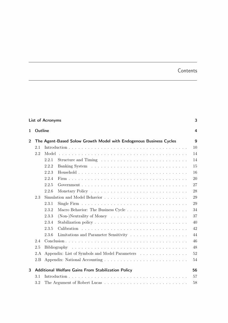
Juglar -type cycles. Moreover, the model generates a short-run Phillips-curve relationship,long-run neutrality of monetary policy and business cycle patterns similar to the Goodwin(1967) model. Fiscal stabilization policy is shown to dampen macroeconomic fluctuations,thus allowing for a higher level of average employment. Calibration of model parameters isconducted to generate realistic orders of magnitude of important macroeconomic proportions.The newly developed model is a combination of ideas from different economic perspectivesand contributes to macroeconomic model-building under the paradigm of agent-based compu-tational economics. The article demonstrates the usefulness of ACE model-building in generaland of the presented demand-led growth model in particular.This chapter is based on my single-authored paper “The Agent-Based Solow Growth Model
with Endogenous Business Cycles”.
Chapter 3: Stabilization Policy
A topic closely related to business cycle dynamics is macroeconomic stabilization policy. Todetermine the possible welfare gains from such policies to society, we adapt the approach ofLucas (2003) with a risk-averse representative agent. However, instead of using a GeneralEquilibrium model, we apply an agent-based macro model, thus relaxing the assumption ofperfect ex ante coordination brought about by the Walrasian auctioneer. We find that theACE macro model allows for a higher average level of employment, if economic activity isstabilized. As a result, the welfare gain of a perfect stabilization at full employment levelis by orders of magnitude higher compared to Lucas’ estimate, who implicitly assumes thatstabilization means dampening both, booms and recessions, in a symmetrical way. The welfaregain under the ACE paradigm consists not only of reduced variability, but also in a higheraverage level of consumption and output.This chapter is based on a joint article with Matthias Lengnick. The initial idea was
developed by Matthias, whereas my contribution consisted of programming the adjustment ofthe ACE model, as well as application and analysis of 1000 replications of both model types.The (short) article was written by both authors in collaborative work.
Chapter 4: Business Climate
Certainly, there are real causes beyond psychology that originarily cause macroeconomic fluc-tuations, like stochastic exogenous shocks in real business cycle theory; or endogenous ag-gregate dynamics emerging in the interaction of economic agents as described in chapter 2.These real causes may create some variability of demand and output in the first place, but un-doubtedly, upward and downward movements are reinforced by expectations. Confidence andexpectations of consumers and firms play an important role in the generation and dynamicsof business cycles. For example, a firm expecting demand to increase is more likely to invest,thus contributing even more to the increase of aggregate demand. Moreover, expectations ofagents are influenced by other agents’ expectations, thus linking the formation of expectations

Outline 6
with regard to economic prospects closely to the pattern and intensity of actually observablebusiness cycles.Processes of social opinion formation might be dominated by a set of closely connected
agents who constitute the cohesive ‘core’ of a network and have a higher influence on theoverall outcome of the process than those agents in the more sparsely connected ‘periphery’.In this chapter, it is explored whether such a perspective could shed light on the dynamicsof a well known economic sentiment index (ZEW survey). To this end, it was hypothesizedthat the respondents of the survey under investigation form a core-periphery network. In adiscrete setting, those agents defining the core were identified, whereas in a continuous setting,the proximity of each agent to the core was determined. As it turns out, there is significantcorrelation between the so identified cores of different survey questions. Both the discrete andthe continuous cores allow an almost perfect replication of the original series with a reduceddata set of core members or weighted entries according to core proximity. Using a monthlytime series on industrial production in Germany, experts’ predictions with the real economicdevelopment were also compared. The core members identified in the discrete setting showedsignificantly better prediction capabilities than those agents assigned to the periphery of thenetwork.This chapter is based on a joint paper with Thomas Lux published under the title “Iden-
tification of a Core-Periphery Structure Among Participants of a Business Climate Survey –An Investigation Based on the ZEW Survey Data” in European Physical Journal B 84 (2011),pp. 521 – 533. Prof. Lux came up with the initial idea to apply a core-periphery networkanalysis to ZEW data, gave valuable advice and suggestions throughout the process. My con-tribution to this paper consisted of handling and utilizing the raw data set, application andadjustment of algorithms and discussion and determination of further steps in coordinationwith Prof. Lux. The draft of the article was also written by me.
Chapter 5: Empirical Growth Analysis
The article “Growth Determinants Across Time and Space – A Semiparametric Panel DataApproach” empirically analyzes worldwide data on economic growth and its determinants. Apanel data set covering 145 countries between 1960 and 2010 has been investigated closely byusing models of parameter heterogeneity. The Functional Coefficient Model (FCM) introducedby Cai, Fan and Yao (2000) allows estimated parameters of growth determinants to vary asfunctions of one or two status variables. As a status variable, coefficients depend on the levelof development, measured by initial per capita GDP. In a two-dimensional setting, time is usedas an additional status variable. At first, the analysis is restricted to bivariate relationshipsbetween growth and only one of its determinants, dependent on one or both status variablesin a local estimation. Afterwards, the Solow (1956) model serves as a core setting of theory-based control variables, while functional dependence of additional explanatory variables isinvestigated. While some constraints of this modeling approach have to be kept in mind,functional specifications are a promising tool to investigate growth relationships. Moreover,

Outline 7
it contributes to an assessment of robustness and sensitivity of uncovered determinants ofgrowth to alterations in the covered period and in the composition of countries in cross-country growth regressions. At the end of this chapter, a simple derivation of FCM calledlocal mean values provides a suitable way to visualize macroeconomic or demographic patternsacross two dimensions in a descriptive diagram.This chapter is based on my single-authored paper “Growth Determinants Across Time and
Space – A Semiparametric Panel Data Approach” published as Economics Working Paper2014-11, University of Kiel, September 2014. Helmut Herwartz provided initial help andsome valuable comments and suggestions at intermediate stages of the article creation.
Chapter 6: Innovation and Patent Analysis
A major source of technological progress in models of endogenous growth is innovation. Inaddition, the private sector’s ability to pursue profitable and sustainable innovation activityis supplemented and supported by public research efforts, which uncover basic knowledgeor base technologies and provide education as a prerequisite for constructive innovation andenhancements. However, the economic significance of ideas and products generated by inno-vation is sometimes difficult to measure sharply. Patenting activity as an observable subsetof overall innovation activity can be illuminated by analyzing patent databases.In a recent research project at the institute of innovation research (University of Kiel)
in cooperation with the German federal ministry for education and research (BMBF), thePATSTAT world wide patent database was searched for patents assigned to publicly financedresearch organizations (PROs) in Germany. Prof. Walter and his research team, includ-ing myself, investigated the characteristics and diffusion of knowledge uncovered by GermanPROs, in particular the diffusion of patented knowledge and its economic relevance to the pri-vate sector. A shortened part from the research projects’ final report (Walter, A. (edt., 2014):"Wirtschaftliche Bedeutung des patentierten grundlagenorientierten Wissens in Deutschland",Hannover: Technische Informationsbibliothek Hannover, pp. 74–104), written in German lan-guage, is attached as chapter 6, covering descriptive statistics of the patent portfolio of GermanPROs and investigating knowledge diffusion by utilization of data on patent citations. Mycontribution to this part of the final report is particularly important. It required severalmonths of sometimes automated, sometimes manual work to recognize and determine about700 different institutions as German PROs as well as firms from numerous countries in the rawpatent data with all the inaccuracy and weakness attached to it, by means of SQL databasesearch. This time-consuming determination of a subset of worldwide patenting activity wasthe basis also for more elaborate statistical analyses within the research project. The excerptpresented in chapter 6 was drafted by myself and consists of a descriptive analysis of thedetermined PRO patent data set.A main finding is that public research appears to generate a stronger economic impact in
Germany, if the respective research area overlaps with technological fields, that are charac-terized by comparative advantages and research focuses of the private sector in Germany.

Outline 8
Appendices
Cited references are listed at the end of each chapter, since the overlap between the chapterswith regard to literature is rather limited. Similarly, lists of symbols that have been introducedin an article are positioned at the end of the respective chapter. However, such lists of symbolsare available only for chapters 2, 3 and 5, where a non-negligible number of symbols is used.

CHAPTER 2
The Agent-Based Solow Growth Modelwith Endogenous Business Cycles
Ulrich StolzenburgDepartment of Economics, University of Kiel
Abstract: This article describes a simulated monetary macro model with different types of interacting agents.As such, it is assigned to the field of agent-based computational economics (ACE), where agents become vir-tual objects in a computer simulation. The ACE model core with labor market and goods market interactionbetween households and firms is adopted from Lengnick (2013), whereas production technology and techno-logical progress of firms are adopted from the neoclassical Solow (1956) model. Nominal interest rates areset in accordance with the Taylor (1993) principle, characterized by strong responses of monetary policy todeviations from inflation target. Although inflation desirably follows lagged output in a pro-cyclical manner,the dynamic system allows for long-run stability of inflation rates. Firms on aggregate level endogenouslygenerate waves of higher and lower investment. A recurrent cyclical movement of aggregate economic activ-ity, in particular demand, employment and inflation, is transmitted from these waves of investment activity.Cyclical patterns of boom and bust emerge with a frequency of approximately seven years just like Juglar -typecycles. Moreover, the model generates a short-run Phillips-curve relationship, long-run neutrality of monetarypolicy and business cycle patterns similar to the Goodwin (1967) model. Fiscal stabilization policy is shownto dampen macroeconomic fluctuations, thus allowing for a higher level of average employment. Calibrationof model parameters is conducted to generate realistic orders of magnitude of important macroeconomic pro-portions. The newly developed model is a combination of ideas from different economic perspectives andcontributes to macroeconomic model-building under the paradigm of agent-based computational economics.
Also available as: Economics Working Papers 2015-01, University of Kiel.

The Agent-Based Solow Growth Model with Endogenous Business Cycles 10
2.1 Introduction
Agent-Based Computational economics (ACE) developed recently as a new branch of macroe-conomic modeling, which falls in the paradigm of complex adaptive systems (Tesfatsion, 2003).Economic agents become artificial objects in a computer simulation, which interact accordingto behavioral rules (Page, 2008). A newly developed ACE macro model is outlined in thisarticle.A key advantage of the ACE approach should be underscored here, which is that analytic
tractability is not a key requirement for model equations. There is no need to solve them foran equilibrium equation or set of equations, thereby forcing assumptions to be overly simple,well behaved and tractable. Instead, model outcome is analyzed by observation of emergenttime series. As a result, modeling of agent behavior becomes less restricted and allows toincorporate and combine research findings from neighboring fields such as experimental eco-nomics and behavioral economics. Another advantage of agent-based models in general is thatmacro results may occur that differ completely from disaggregate micro level agent behavior.A famous generally understandable example for such an emergent property on aggregate levelis Schellings (1969) model of racial segregation in cities, emerging from rather open-mindedindividual attitudes with regard to mixed neighborhoods.There are some disadvantages to acknowledge: First, it requires a good deal of effort to get
familiar with programming and typical challenges of calibrating these models. Oeffner (2009)provides a detailed and comprehensible introduction to the virtues and challenges of ACEmodel building. Secondly, there is no analytic solution of equilibrium or model dynamics,so people used to it may feel a lack of mathematical certainty. According to Page (2008),ACE models “occupy a middle ground between stark, dry rigorous mathematics and loose,possibly inconsistent, descriptive accounts”. Thirdly, freedom concerning modeling of agentbehavior is accompanied by a growing level of complexity, which complicates understandingand interpretation of results. The term “wilderness of bounded rationality” points to thedifficulty of transferring certain findings about non-rational agent behavior to functional forms.It is accompanied by the problem of (too) many parameters in large models (Sims, 1980). AsLengnick (2013) argues, ACE modelers are “tempted to over-increase the level of complexity”.Until recently, macroeconomic model building is rather dominated by Dynamic Stochastic
General Equilibrium (DSGE) models, which became the standard models of monetary policyanalysis (cf. Woodford, 2003; Clarida et al., 1999). However, DSGE modeling is subjectto ongoing criticism (Mankiw, 2006; Solow, 2010; Colander et al., 2009). Some standardparadigms appear questionable, especially in the light of possibilities offered by the ACEapproach.To begin with, most General Equilibrium models assume existence of a representative agent,
who optimizes utility with infinite horizons. Kirman (1993) argues why the assumption ofa representative agent is questionable. Solow (2010) challenges the idea “that the wholeeconomy can be thought of if it were a single [...] person carrying out a rationally designed,long-term plan, occasionally disturbed by unexpected shocks, but adapting to them in a

The Agent-Based Solow Growth Model with Endogenous Business Cycles 11
rational, consistent way.” He also argues that DSGE models by construction provide noreasonable way to cope with involuntary unemployment, since the representative agent onlyrationally chooses to substitute work with leisure a little more. Moreover, there may also occurthe need to analyze consequences of certain policies with regard to the income distribution;or to analyze how the distribution of wealth influences growth (e.g. Alesina and Rodrick,1994; Dynan, Skinner and Zeldes, 2004; Galor, 2009). The ACE approach allows agents tobe modeled as heterogeneous individuals, who partly can become involuntarily unemployed.Topics related to wealth and income distribution can also be tackled.Another assumption in general equilibrium models is that relative prices are simply set op-
timally, thus allowing for permanent market clearing as long as no frictions are imposed. Theconcept of permanent fulfillment of an equilibrium condition, brought about by a fictitiousWalrasian auctioneer, who calculates an optimal vector of relative prices in meta time, is notconvincing (Ackerman, 2002; Gaffeo et al., 2008; Kirman, 2006). In ACE models, the processand coordination of relative price adjustments can be modeled explicitly, possibly resultingin a temporary equilibrium situation. Finally, the famous Lucas (1976) critique argues thatrelations between macroeconomic variables may change with policy, because agents incorpo-rate new policies into economic decision making. This idea induced not only the spread ofmicrofoundations as an acknowledged requirement for macro models, it also made the ratio-nal expectations hypothesis a key ingredient of model building. As long as the consequencederived from Lucas’ critique concerns the requirement of microfounded agent behavior, ACEmodels allow for a much more complex and realistic set of assumptions applicable to simu-lated heterogeneous agents. However, an application of rational expectations to ACE modelsappears inappropriate, since it implies that (simulated) agents are able to fully understand acomplex dynamic system of agent interactions and to calculate expected values for aggregateoutcomes. Not even the designer of the dynamic ACE system is able to calculate an accurateprobability distribution of possible outcomes. A more general critique of rational expectationsin macro models is provided by Syll (2012).It should be noted that former arguments do not disqualify DSGE models to analyze and
estimate real aggregate economic behavior in a valuable way. Friedman (1951) argues thataccuracy of predictions derived from a theory is more important than the underlying assump-tions, as long as they are consistent. Nevertheless, the goal of economic theory is not restrictedto prediction and data-fitting; it also consists of providing convincing explanations of real-world phenomena and processes, so contrary to Friedmans claim assumptions actually domatter. The ACE approach offers a new way for macroeconomic model building, facilitatingmore realistic designs of agent behavior.Point of departure for the newly developed ACE macro model is the baseline model of
Lengnick (2013), later referred to as L13 model.1 It is a simple model of a closed economy,which partly draws on former models of Dosi et al. (2008) and Gaffeo et al. (2008). The
1 Java Source code of the Lengnick model was adopted, which was very helpful and facilitated the start. Programoutput such as macroeconomic time series were analyzed with MATLAB. The source code of the extendedmodel described here is available upon request.

The Agent-Based Solow Growth Model with Endogenous Business Cycles 12
simulated economy consists of households and firms interacting on a goods market and on alabor market, where each type of agent follows simple adaptive rules. The model generatesendogenous business cycles and some desired characteristics on aggregate level.2 The basicstructure of the model has been adopted, such as the sequence of activities, connectionsbetween agents and the organization of the goods market and of the labor market.Certain restrictions of the Lengnick model prompted several changes and extensions: (1)
Labor is sole production factor input in L13, while in the extended model each firm is endowedwith a capital stock, which is subject to depreciation. Technological progress in combinationwith Cobb-Douglas production technology is incorporated, so that firms become customersof other firms by purchasing investment goods. This extension simply forces productiontechnology and architecture of the Solow-Swan growth model (Solow, 1956; Swan, 1956) onsingle firms of an agent-based framework.3 (2) In L13, firm ownership remains unspecified.Here, households are shareholders of firms, so that profit is paid out as a return rate of firmshares. (3) In L13, firms are frequently unable to meet customer demand, followed by a lossof customers. To prevent a constant flow of restricted, disappointed customers between firms,firms are modeled with excess production capacity in the new model. (4) A fixed quantity ofmoney is circling between agents in L13. Instead, endogenous money is introduced with credit,savings, interest rates and a monetary policy rule. Availability of credit also avoids frequentemergency wage cuts of firms, if they run out of money in L13. (5) Finally, consumptionpaths of unemployed households in L13 are unrealistic, since consumption almost immediatelydrops to low one-digit percentages of former levels. The new model introduces a government,providing for unemployment benefits and collecting taxes.The presented monetary model incorporates elements from different economic schools: It
is Keynesian, since economic activity of firms is strictly demand-driven and features involun-tary unemployment, while there is no hypothetical lower wage that allows for market-clearing.Say’s law does not apply, when firms are designed to have excess production capacities, thusallowing for unsold quantities. Fluctuating consumption and investment, combined with un-known household savings and availability of credit weaken the link between production andaggregate demand even more. In the context of this model, the notion of “equilibrium” maybe understood as a situation when aggregate demand fluctuates around a target percentage ofproduction capacity. Business cycles are created endogenously, generated by higher or lowerfirm investment as the leading determinant of economic dynamics. Both Keynes (1936) andKalecki (1937) also uncovered investment as a major source of periodical macroeconomic fluc-
2 Crises in the L13 emerge as follows: After a period of abundant aggregate demand, firm inventories decline tocritical lower values. Firms are permanently unable to acquire more workers for production enlargement, thusinducing rising wages and correspondingly decreasing profits. As soon as profits reach a lower bound, priceincreases are triggered, by which the money supply is devalued in a system with a fixed quantity of money.Finally, the reduced value of real money in the system causes a drop in firm sales, which induces firms to fireworkers.
3 To name a few major differences of the Solow model: It only captures the aggregate level and assumes allfactors of production to be constantly employed; there is no role for money; savings are generated as a fixedproportion of output and are directly invested.

The Agent-Based Solow Growth Model with Endogenous Business Cycles 13
tuations. As it turns out, firm profits depend on aggregate investment, but not on investmentof the one single firm. On the other hand, firm investment in turn depends on past firm profits.A reinforcing spiral of investment, demand and profits is an emergent property on aggregatelevel, both upwards and downwards. As it turns out, the emergent cyclical pattern resemblesdynamics of the Goodwin (1961) model. Elements from neoclassical theory are incorporated,namely the Solow-Swan growth model from which firm technology and technological progressare adopted on firm level. Monetary policy is conducted in accordance with the New Macroe-conomic Consensus where the Taylor principle is applied to automatically adjust nominalinterest rates as a strong response to deviations from inflation target. A short-run Phillipscurve emerges from aggregate model dynamics, similar to New Keynesian models.Naturally, there have been other approaches to ACE macro modeling before. Lengnick
(2013) distinguishes two categories of such models: The first category models the economyin considerable detail and complexity such as the EURACE project (Dawid et al., 2011) witheven a spatial structure. The second category abstracts from reality to a larger degree, whichis where L13 and the presented model belong to. Dosi et al. (2008) develop a model ofinvestment with R&D, where aggregate demand and output are driven by lumpy investment.They obtain macro behavior in line with a number of stylized facts. However, contrary to theapproach followed here, neither a labor market nor a goods market are modeled, instead firmsare simply assigned a proportion of aggregate demand. Moreover, households fully consumetheir income, which also differs from the more general consumption decision applied here.Gaffeo et al. (2008) explicitly model the goods market, but do not capture the capital sideof the economy, since their production function employs labor as the sole input. Oeffner(2009) develops an ACE macro model characterized by demand-driven economic activity,business cycles amplified by firm investment, Cobb-Douglas technology, growth and inflation.It resembles in many ways the model presented here. However, it simulates three firm sectorsinstead of one: Two consumption goods sectors (with a capital stock) and a capital goodssector (modeled without a capital stock); each of them populated by a fixed number of firms.Another major difference is that firm employment is fixed in Oeffners model, so there is noanalysis of unemployment.The ACE model presented here is the first to combine an explicit modeling of goods market
and labor market, firm capital stock, investment, growth, inflation and endogenously createdbusiness cycles. Contrary to numerous other models, it encompasses the demand-led characterof firm decisions on employment and price setting. This article provides a comprehensivedescription of the model structure and analyzes simulation behavior. As will be shown, themodel reproduces a number of stylized facts and is calibrated to generate realistic proportionson aggregate level. To further demonstrate the usefulness of ACE models in general and ofthis extended model in particular, the response to a monetary shock is analyzed. Additionally,three different fiscal policy regimes are analyzed: As it turns out, a policy aiming at demandstabilization performs best with respect to average employment. Yet this result, admittedly,is a rather expectable property of a demand-led macro model.

The Agent-Based Solow Growth Model with Endogenous Business Cycles 14
The remainder of this article is organized as follows: Section 2.2 explains the building blocksof the agent-based economy step-by-step, such as the basic structure, banking system, agentclasses of households, firms and the government as well as the conduct of monetary policy.Section 2.3 describes the model behavior in the running simulation. Time series for individualfirms (2.3.1) are followed by macroeconomic variables and analysis of business cycle dynamics(2.3.2). In addition, Phillips curves, monetary policy shocks (2.3.3), fiscal policy (2.3.4),calibration issues (2.3.5) and limitations (2.3.6) are also treated in this chapter. Section 2.4concludes.
2.2 Model
2.2.1 Structure and Timing
The sequence of activities consists of in two different time intervals (cf. Lengnick, 2013).All relevant decisions take place on a monthly basis, as well as payment of wages, profits,interest, taxes and unemployment benefits. On daily basis, goods are only produced and soldto customers. Figure 2.1 provides an overview of the sequence of important activities.
Figure 2.1: Sequence of monthly events.
The developed monetary model distinguishes carefully between real variables, which arecounted in natural units (goods), and nominal measures counted in currency units. Regardingnotation, all nominal measures are written consequently with a preceding letter n in order toavoid confusion, while real measures are written without this preceding letter.4 The modelinternally calculates on a monthly basis, so that inflation rates, interest rates, the depreciationrate and return rates are actually very small values. In this article, however, correspondingvalues are presented as annualized percentages in order to simplify understanding. In the
4 The only exception is the nominal interest rate it, which is measured as a percentage, so it is actually not anominal variable with respect to its unit of measurement.

The Agent-Based Solow Growth Model with Endogenous Business Cycles 15
following sections, variables are in monthly notation with a subscript t with months t =
1, ..., T .There are three types of agents: households, firms, and a government sector (state). The
number of households (Nhh = 2000) and firms (Nfi = 100) is fixed in order to excludedemographic aspects as well as firm entry and exit. A central bank is also present, but has noother function but to set the nominal interest rate. Figure 2.2 depicts the model structure.
Figure 2.2: Model structure with financial and real flows between agents.
2.2.2 Banking System
All households, firms and the government are endowed with a bank account. There is only onebank representing the banking system. However, it is abstracted from administration costs,employees and the objective to generate profits. Each bank account contains a money account,which is used for payments5, and a savings account, which can be used as an interest-bearingfinancial asset; and which can also become a credit account, if the balance is negative. Themoney account is restricted to positive values and it is interest-free. The savings account canbe positive and negative, so it is either a financial asset or a credit account.All agents are free to transfer arbitrary amounts from the money account to the savings
account and back, so there is no credit restriction and no credit risk evaluation. Money5 The model abstracts from cash payments, so deposits of the money account are transferred between agentsin order to execute payments. The two-staged structure of real-world banking systems with a role for centralbank money is also not captured.

The Agent-Based Solow Growth Model with Endogenous Business Cycles 16
is created endogenously once an agent demands for additional liquidity, thereby increasingaggregate money. The created monetary amount is used for payments, thus circling betweenagents. Once it is transferred to a savings account, the aggregate quantity of money is reducedrespectively.6 At the start of each month, agents decide about their liquidity need, so theydecide to hold transaction money based on their past monthly cost. Spare money is moved tothe savings/credit account, either to gain interest income (households) or to avoid unnecessarycost (firms).All Money and savings accounts sum up to zero at all times.7
0 = nMhht + nMfi
t︸ ︷︷ ︸transaction money
+nSChht︸ ︷︷ ︸+
+nSCfit︸ ︷︷ ︸−
+nSCstt︸ ︷︷ ︸−
, (2.1)
Aggregate money and savings/credit accounts of the household sector and firm sector aresimple aggregates: nMhh
t =∑Nhh
h=1 nMhht,h , nM
fit =
∑Nfi
i=1 nMfit,i , nSC
hht =
∑Nhh
h=1 nSChht,h and
nSCfit =∑Nfi
i=1 nSCfit,i. The government does not hold any transaction money at trading
days. Therefore, nM stt = 0.
The interest rate is adjusted monthly by a central bank. It is imposed on all savings/creditaccount balances and is paid by debtors and received by creditors of the bank. For simplicity,the current nominal interest rate is valid for the whole stock of savings and credit.8
2.2.3 Household
Job Market
Job market decisions take place at the beginning of a month. Each household is connected toone employer unless he is unemployed, while a firm is able to employ an arbitrary number ofemployees. Households offer inelastically one unit of labor per month, so that wage paymentis monthly labor income. Each firm pays the same wage to all of its employees, though theremay be differences between firms.If a household is fired, it will remain employed during the current month and becomes un-
employed at the beginning of the following month. A reservation wage, which is the minimum
6 Concerning double bookkeeping, money is created in a credit contract, once an indebted firm asks for morecredit, which is a balance sheet extension. If a household transfers an amount of money from its savingsaccount to the money account, it is a mere asset swap. Both ways, aggregate money is increased. On theother hand, the quantity of money is reduced if a firm transfers it to the savings/credit account in order topay back debt, which is a balance sheet contraction. A household transferring money to its stock of savingsis experiencing an asset swap again. The aggregate quantity of money is decreased in both cases.
7 Firms and the government are usually indebted, so they are debtors of the banking system. Householdsaccumulate savings, so they are creditors of the banking system. Money holders (households and firms) arealso creditors.
8 In a more complex setting, savings and credit are modeled as financial contracts featured by a contract durationof a fixed number of months. This is actually more plausible, since firms consider investments dependent onthe current nominal interest rate and expected inflation. An investment decision financed by a fixed creditcontract at least preserves decisive credit conditions.

The Agent-Based Solow Growth Model with Endogenous Business Cycles 17
Figure 2.3: Household Connections: Seven firms as trading partners for consumption goods (arrows) and oneemployer (dashed line).
wage for acceptance of a new job, is set at its latest wage payment. Each month of unsuc-cessful job search reduces the reservation wage by 5%, which is effectively a small obstacle toemployment. The household contacts up to five firms per month to ask for a job. As soon asa firm offers a job, for which the wage exceeds the current reservation wage, the household isemployed instantly. With a probability of 10%, an employed household will also contact onefirm to ask for a better-paid job. These job offers are refused directly, if the new wage is lowerthan the current one. If the offered wage is higher, the job is accepted with a probabilitydependent on the wage difference according to Prob(Accept) = 1− e−γw·ln(2)·∆nW (see Figure2.4), which ensures a restricted level of wage competition.
0 10 20 30 40 500
20
40
60
80
100
Price / Wage Difference (%)
Sw
itch
Pro
babi
lity
(%)
γ = 5
Figure 2.4: Household decision: Probability to change employer (supplier) dependent on wage (price) difference.
Income and Taxes
All monthly payments to households will be carried out at the end of a month, thus deter-mining household income for the following month. Primary income consists of up to threesources: (1) wage from employer i, (2) paid-out profit of firms the household is shareholder ofand (3) nominal interest payment on nominal savings/credit account nSCt,h. If a householdis indebted, nSCt,h and interest payments are negative.
nIncprimt,h = nWt,i + nΠpaidt,h + it · nSCt,h (2.2)

The Agent-Based Solow Growth Model with Endogenous Business Cycles 18
A tax rate τt is imposed equally on all sorts of primary income: nTaxt,h = τt · nIncprimt,h .Unemployment benefits (nUBt) are paid if the household was unemployed during the runningmonth. Instead of wage, it receives unemployment benefits, which is 50% of net average wage:
nUBt = 0.5 · (1− τt) · nWIt−1, (2.3)
where nWIt−1 is the average wage (or the wage index), calculated as a mean value of previousmonth’ firm wages, weighted by the employment share of each firm.9 Household h is left withnet income
nIncnett,h =
(nWt,i + nΠpaid
t,h + it · nSCt,h)· (1− τt) if employed(
nΠpaidt,h + it · nSCt,h
)· (1− τt) + nUBt if unemployed
(2.4)
Goods Market Trading Partners
Each household maintains a fixed number of seven connections to firms (cf. Lengnick, 2013).Firms, on the other hand, are not limited in the number of connections to customers. Con-nections to supplying firms are adjusted slowly and infrequently, thus expressing loyalty ofcustomers and stability of trading relations. Nevertheless, each household adapts its list offirm connections monthly due to price consideration, customer restrictions and randomly.
1. With a fixed probability of pp = 25%, households search for cheaper trading partners.One existing (old) connection is chosen randomly, and one other (new) firm is also chosenrandomly. If the new price is higher than the old price, the existing connection is kept.Otherwise, the price difference is translated into a probability to replace the existingconnection: Prob(Switch) = 1−e−γp·ln(2)·∆P (see Figure 2.4). This way, imperfect pricecompetition is established, but customers do not react strongly when price differencesare negligible.
2. If a firm is sold out, it is unable to satisfy further customer requests. In the respec-tive trading day, restricted customers simply buy from the next firm. However, beingrestricted more often by the same firm induces households to replace the respectivetrading connection. Again, with a probability pr = 25% one (restricted) connectionis reconsidered and eventually replaced by a random new firm. The probability for aswitch is dependent on the severeness of the restriction compared to consumption plans,while negligible restrictions will have no consequences.10
3. Finally, trading connections are exchanged randomly with a low percentage of ps = 2%.With a sum of 2, 000 · 7 = 14, 000 firm connections, random rearrangement concerns 40
9 nWIt−1 =∑Nfi
i=1 nWt−1,i · Lt−1,i∑Nfij=1 Lt−1,j
10Restrictions of demand are measured in daily consumption packages: RDt. Probability to change a connectiondepends on last month’ restriction: Prob(Switch) = 1− e−γr·ln(2)·RDt−1 . Restrictions by more than one firmwill induce replacement of one connection dependent on the relation of the restriction between the two (ormore) restricting firms.

The Agent-Based Solow Growth Model with Endogenous Business Cycles 19
connections per months. This random customer redistribution ensures that small firmsdo not run out of customers but are stabilized at some point.
Consumption
Simulated households plan consumption based on current income, not taking into consider-ation the stock of savings, which may be a multitude of income. However, it is assumedthat households offset expected real devaluation of savings stocks (nSCt,h · πet ) by directlyreinvesting the respective amount, where πet is expected inflation (as defined below in section2.2.4). Therefore, consumption-relevant net income is reduced, so that interest income is onlyrelevant for consumption, as long as it is generated by the real interest rate rt.11 A personalprice index nPIct,h, which is the average price of current trading partners, is calculated todetermine the purchasing power of individual income. Consumption-relevant real net incomeis therefore
RNIt,h =nIncnett−1,h − nSCt,h · πet
nPIct,h(2.5)
All households are assigned a common intercept parameter Ct and a common marginalrate of consumption c.12 Consumption also depends negatively on the expected real interestrate rt = it − πet , which is not only plausible, but also derived from optimizing behavior ofrepresentative agents in DSGE models like Woodford (2003).Households plan real consumption at the beginning of each month.13 It is strongly affected
by latest consumption, so it adjusts only gradually to a new income level, modeled with aparameter of consumption inertia λc = 0.9. Therefore, a household adjusts at a monthly rateof (1 − λc) = 10% to a new income level, for example if there is a change in employmentstatus. Planned real consumption of household h is:
Ct,h = λc · Ct−1,h + (1− λc) ·(Ct + c · e−rt ·RNIt,h
)(2.6)
11Oeffner (2009) went further and made interest payments reinvested completely, not only the part of nominalinterest that offsets inflationary devaluation. He argues at length why reinvestment of interest paymentsis a crucial stability condition for the simulated economy. Otherwise, a rising interest rate would increasehousehold income and induce higher consumption expenditure, so that economic activity were counter-factuallystimulated by “tight” monetary policy.
12A simple linear Keynesian consumption function is adopted here as explained in Mankiw (2000, p. 480).Parameter c = 0.85 reflects the marginal propensity to consume, whereas the intercept parameter is set at asmall share of previous month’ net average wage: Ct = 0.18 · (1− τt) · nWIt−1, therefore the intercept growsat the same rate as the entire economy.
13Usually, planned real consumption becomes actual real consumption. If one of the randomly chosen tradingpartners is sold out, the household simply chooses randomly the next firm out of 7 (see section 2.2.3) to satisfyits daily demand. Since all firms provide excess production capacities, it practically never happens that ahousehold is restricted completely by all seven firms, even if the case is a theoretical possibility.

The Agent-Based Solow Growth Model with Endogenous Business Cycles 20
2.2.4 Firm
Technology
Firms employ Cobb-Douglas production technology with factor inputs capital Kt,i, labor Lt,iand technology parameter At. Daily production capacity of firm i with capital exponentα = 0.2 is: Y c,day
t,i = Kαt,i · (At · Lt,i)
1−α. Thus, monthly production capacity multiplies theformer equation by 30 days per month:
Y ct,i = 30 ·Kα
t,i · (At · Lt,i)1−α (2.7)
Technology parameter At is identical for all firms and grows at a constant exogenous rate oflabor-enhancing technological progress gA = 1.2% annually (or 0.1% per month), so At =
At−1 · egA (cf. Barro and Sala-i-Martin, 2003, chapter 3).
Capital Stock Development
In contrast to the original Lengnick (2013) model, each firm not only acts as a supplier butalso as a customer of goods and services, when it invests in real capital. There is no dis-tinction between consumption goods and investment goods.14 Investing firms and consuminghouseholds contribute to a unique demand flow. To purchase goods or services for investment,each firm maintains a limited number of seven connections to other supplying firms. Thesesupplier connections are reconsidered monthly equivalent to household connections in sec-tion 2.2.3 with regard to prices, restrictions and randomly. At the beginning of each month,connections are reconsidered and replaced with some probability.
Figure 2.5: Firm Connections: Number of trading partners for investment goods supply is limited to 7, numberof employees (households) and customers (households and firms) is not limited.
14The same implicit assumption is part of the Solow (1956) model, where aggregate output is split into investment(s · Y ) and consumption.

The Agent-Based Solow Growth Model with Endogenous Business Cycles 21
Each firm maintains a stock of real capital goods, which is devalued by parameter ρ at theend of each month at an annual rate of 9.6% (or monthly 0.8%). A firm invests accordingto its monthly gross investment plan, which is discussed later (see section 2.2.4). On a dailybasis, each firm purchases goods from other firms to accomplish its investment plan. As soonas the month has passed, the sum of newly purchased investment goods is added to the capitalstock. It is ready for productive use in the following month. Firm capital evolves accordingto
Kt,i = Kt−1,i + It−1,i − ρ ·Kt−1,i︸ ︷︷ ︸Inett−1,i
(2.8)
Key Data for Firm Decisions
Firm decisions are built upon few key variables, some of which are explained here:Utilization: Capacity utilization is defined as real sales divided by production capacity:
Ut,i =Y salest,i
Y ct,i
(2.9)
In order to prevent supply shortages with a likely loss of trading relations to customers, firmsprovide for excess capacity. The target value U∗ is 85%, permitting firms to accommodatedemand fluctuations.15 Prices are set such that they offset cost of temporarily idle resources.For decision-making, firms determine a short-run weighted average level of utilization of lastTu = 6 months, where weights are highest for the most current month and decline linearly:
U t,i =
Tu∑s=1
Ut−s,i ·(Tu + 1− s)
0.5 · (Tu · (Tu + 1))(2.10)
Expected Inflation: Inflation is measured by the price index PIt which is a mean priceof all Nfi = 100 firms in month t, weighted by their (real) market shares:
nPIt =
Nfi∑i=1
nPt,i ·Y salest,i∑Nfi
i=1 Ysalest,i
(2.11)
Annual inflation is the logarithmic difference of the price index with 12 months lag:πt = (ln(nPIt)− ln(nPIt−12)). Annualized monthly inflation is the logarithmic differenceof neighboring values of the price index: πmt = 12 · (ln(nPIt)− ln(nPIt−1)).For simplicity, inflation expectations are homogeneous among all agents. It is assumed that
medium-run expected inflation is adaptive based on the last T π = 24 monthly inflation ratesas a weighted mean value with linearly declining weights. It is further assumed that central
15 Idle resources are quite normal: Think of restaurants, empty shops, hotel rooms, or food production. Ap-parently, the degree of utilization of available resources is not 100% in many branches, but on average wellbelow, particularly in the service sector. Moreover, consumption goods are often short-lived (food), go out offashion or out of date (clothes, electronics) and are costly to store. Respective firms will have to deal withidle resources and emergent cost of produced goods that can not be sold immediately.

The Agent-Based Solow Growth Model with Endogenous Business Cycles 22
bank announcements of the inflation target π∗ influence expectations directly to a some extentwith λπ = 0.1 reflecting central bank credibility. Expected inflation is
πet = λπ · π∗ + (1− λπ) ·Tπ∑s=1
πmt−s ·(T π + 1− s)
0.5 · T π · (T π + 1)(2.12)
Profit Rate: Let return on capital (RoC, elsewhere also termed h, e.g. in Hein andSchoder, 2011) relate profit with capital stock value. In order to assess profitability per unitof invested capital, nominal interest payments on firm debt are left out of the calculation.Therefore, return on capital is calculated by subtracting costs of wages and capital depreci-ation from firm turnover, and to divide it by the current capital stock, valued by the meanprice nPIKt,i of currently connected suppliers of investment goods:
RoCt,i =nPt,i · Y sales
t,i − nWt,i · Lt,i − ρ ·Kt,i · PIKt,iKt,i · nPIKt,i
(2.13)
The profit rate of last 12 months RoCt,i is calculated as a simple mean value of monthlyprofit rates. Firm decisions for investment also consider the development of the profit rate, inparticular the difference between RoCt,i and the average profit rate 12 months before, whichis RoCt−12,i.
Decision: Price
Firms adjust their prices only infrequently as a result of menu costs. The current firm marketprice nPt,i is accompanied by a target price nP ∗i which reflects the exact price the firm wouldbe willing to choose in the absence of menu costs. If the target price deviates by more than (anarbitrary threshold of) 1.5% from the current market price, the firm sets the current targetprice as a new market price.
nPt,i =
nPt−1,i ifnP ∗t,i−nPt,i
nPt,i∈ (0.985; 1.015)
nP ∗t,i else(2.14)
Similar to the Calvo (1983) model, this price setting behavior ensures that only a fraction offirms changes its price in a certain period. However, unlike the Calvo approach, where firmsare forced to wait for a random event (the “Calvo fairy”) to finally being allowed to adjustthe price, firms decide freely about the timing of price adjustments here.The target price evolves monthly with expected inflation and capacity utilization: With
a high level of capacity utilization, a firm is more likely and willing to increase the price,considering itself in a strong market position. Deviations below target utilization triggerprice drops, utilization above target leads to a rising target price. The probability of anadditional target price movement is modeled with a random decision, whose probability isgiven by a reversed bell curve with standard deviation σ = 0.14 as shown in Figure 2.6. The

The Agent-Based Solow Growth Model with Endogenous Business Cycles 23
price change decision is given by:
DPt,i =
1 if (U t,i − U∗ ≥ 0) with Prob = 1− e
−(Ut,i−U
∗
σ
)2
−1 if (U t,i − U∗ < 0) with Prob = 1− e−(Ut,i−U
∗
σ
)2
0 with Prob = e−(Ut,i−U
∗
σ
)2
(2.15)
70 75 80 85 90 95 1000
10
20
30
40
50
60
Latest Capacity Utilisation (%)
Pric
e C
hang
e P
roba
bilit
y (%
)
Shadow Price down Keep Price Shadow Price up
Figure 2.6: Probability to change the firm shadow price. When capacity utilization is low, price is likelydecreased, for high utilization, price is likely increased.
Then, the target price is actually moved up or down by εp, which again is a random variablethat follows a uniform distribution between 0% and 1.5%.16 Therefore, utilization below targetimplies a likely reduction (or slower increase) of the target price. Utilization above target levelimplies a higher probability of additional increases. In the absence of such acceleration of theslow inflationary price drift, an annual inflation of approximately 1.2% leaves the market priceunchanged for more than 12 months on average, before price adjustments are triggered.
nP ∗t,i = nP ∗i · (1 + πet +DPt,i · εp), εp ∼ U(0, 0.015), (2.16)
Please note that deviation of firm utilization from target, U t,i −U∗, is a similar concept asthe output gap in New Keynesian (NK) models. Price setting of an individual firm dependson this “utilization gap” and is effectively a similar mechanism as the New Keynesian PhillipsCurve (cf. Woodford, 2003). Target utilization at 85% of production capacity equates to pro-duction at 100% of the so-called production potential of a representative firm. In NK models,the output gap directly affects inflation with an estimated parameter. Here, deviation fromtarget utilization of a single firm generates price movements only with a certain probability,while on aggregate this stochastic element reliably generates inflation dynamics following eco-nomic activity. One key difference is that NK models assume rational expectations, while thepresented ACE model applies adaptive inflation expectations. However, NK models often use
16Since latest utilization is correlated with neighboring values, a high degree of latest utilization will likely befollowed by another one, so the target price may rise several months in a row.

The Agent-Based Solow Growth Model with Endogenous Business Cycles 24
hybrid Phillips curves which incorporate forward-looking and also backward-looking inflation(hybrid NKPC).
Decision: Hire or Fire
Short-run fluctuations of demand and utilization will be accommodated within a corridor(U low, Uup) around the target value U∗ = 0.85, without any adjustments to production.However, if latest utilization rises to levels above Uup = 0.91, the firm will create an openposition by increasing the employment target L∗t,i. A household asking for a job in that monthis employed immediately, if the firms’ offered wage is high enough for the household to acceptit. On the other hand, if latest utilization falls below U low = 0.78, the employment target isdecreased so that a random worker is fired at the beginning of the following month:
Firm Decision:
L∗t,i = L∗t−1,i − 1 (Fire) U t,i < U low
L∗t,i = L∗t−1,i + 1 (Hire) U t,i > Uup
L∗t,i = L∗t−1,i U low <= U t,i <= Uup
(2.17)
However, if employment of the firm has changed during the last Tu = 6 months, the firm hasto recalculate its degree of latest utilization U t,i with production capacity values based oncurrent employment. Then, firm employment decisions are based on hypothetical values ofpast utilization. For example, if the firm just fired a worker, past sales are compared to nowreduced production capacity.
Decision: Wage
A firm-specific wage contract is fixed for several months. Similar to price setting behavior, atarget wage develops permanently, while the actual market wage is adjusted only infrequently.When a new wage contract is due at time s, the current target wage is set as new firm wage.
nWt,i = nW ∗t,i if t = s (2.18)
The new wage contract runs until month s = t + 10 + ν, while ν follows a discrete uniformdistribution between 0 and 4, so duration for the new contract is a random number between10 and 14 months. Only a part of firms adjusts its wage in each month; average contractduration is 12 months.Owners of the capital stock and workers struggle for their proper share of generated value
added. The development of firm target wages depends on (1) expected inflation, (2) laborproductivity growth, (3) latest utilization (4) the deviation of current markup (of price overunit wage cost) from its target value and (5) whether the firm was able to fulfill its employmenttarget lately. The target wage is adjusted monthly:
1. It is increased by expected monthly inflation, so nW ∗t,i is multiplied by (1 + πet ).
2. The rate of labor productivity growth is a natural part of wage negotiations. The targetwage is therefore multiplied by: (1 + gA)

The Agent-Based Solow Growth Model with Endogenous Business Cycles 25
3. High utilization increases firm profit, so negotiation power of employees increases withhigh utilization. Monthly deviations from utilization target are translated with factorau = 0.05 to changes in the target wage. nW ∗ is multiplied by (1 + au · (U t,i − U∗)).
4. The firm compares wage cost per unit of production with its current market price.Assuming a target value of m∗ = 60% for a markup of price over unit wage cost, thecurrent markup mt,i is closing the gap to its target value m∗ at a rate of am = 3% permonth. The target wage is multiplied monthly by (1 + am · ln(
mt,im∗ )).
5. If the firm was unable to fulfill its employment target L∗t,i in the last month, for examplewhen no household was willing to get hired, the shadow wage is increased by a randomvariable εw, which follows a uniform distribution between 0 and 0.01. If the firm wasable to fulfill its employment target for the past Tw = 6 months, the shadow wage isdecreased by that random variable. Therefore, the target wage is changed additionally,if DWt,i is different from 0:
DWt,i =
1 if L∗t,i > Lt,i
−1 if L∗t−s,i = Lt−s,i, s = 0, 1, ..., Tw − 1
0 else
(2.19)
The target wage is multiplied by (1 +DWt,i · εw) with εw ∼ U(0, 0.01). Note that thislast part of the wage setting mechanism is adopted from Lengnick (2013).
In addition, the target wage evolves according to:
nW ∗t,i = nW ∗t−1,i ·(
1 + πet + gA + au · (U t,i − U∗) + am · ln(mt,i
m∗
)+DWt,i · εw
)(2.20)
Decision: Investment
In the context of investment decisions, hypothetical profit nΠhypt,i is maximized, which ignores
nominal interest payments, but optimizes capital input with respect to the real interest rate:
nΠhypt,i = nPt,i · Y Sales
t,i − nWt,i · Lt,i − (rt + ρ) ·Kt,i · nPIKt,i. (2.21)
nPIKt,i is the mean price of current trading partners for capital investment (which is closeto the general price index nPIt), rt = it − πet is the expected real interest rate. The firmcalculates with output at target utilization U∗:
Y Salest,i ≈ U∗ · Y c
t,i = U∗ · 30 ·Kαt,i · (At · Lt,i)
1−α (2.22)
The capital stock is optimal when the marginal productivity of capital equals its marginalrunning cost, i.e. capital depreciation and real interest payments.
∂nΠhypt,i
∂Kt,i= 0 = nPt,i · U∗ ·
∂Y c
∂K− (it − πet + ρ) · nPIKt,i (2.23)

The Agent-Based Solow Growth Model with Endogenous Business Cycles 26
Rearranging yields the target capital stock:
K∗t,i =
(nPt,i
nPIKt,i· U∗ · 30 · α
(it − πet + ρ)
) 11−α
·At · Lt,i (2.24)
All terms in brackets of equation (2.24) are constant or stable in the long run. Therefore,we see that the target capital depends linearly on labor input Lt,i and technology parameterAt. Once a firm hires a worker, marginal productivity of capital rises, so that K∗ risesproportionally. When employment is constant, At grows at a constant rate gA, so K∗ alsogrows at that rate. For the whole economy, aggregate capital also grows at gA.Investment of a firm depends on (1) capital depreciation, (2) distance to the target capital
stock K∗t,i (3) last years average profit rate RoCt,i and (4) the change in the average profitrate.
1. The base level of gross investment is set by real capital depreciation ρ ·Kt,i.
2. It is multiplied by target capital divided by current capital. The resulting convergence totarget capital also brings about a dependence of current investment on employment Lt,i,current capital Kt,i and real interest rates rt). Constant growth of At also determinesaverage net investment to be positive.
3. The return rate to the capital stock of the last 12 months influences investment, sincecapital is invested where it is most productive and profitable. Gross investment ismultiplied by (1 + ah ·RoCt,i).
4. The development of profit also influences investment, as it was claimed by Kalecki asdescribed by Dobb (1973, p.222). Investment is multiplied by (1 + a∆h · (RoCt,i −RoCt−12,i)). As it turns out, this term strongly determines business cycle dynamics onaggregate level.
Finally, since investment decisions are often carried out with some lag, actual gross investmentis adjusted slowly with an investment inertia parameter λI = 0.9. In sum, planned grossinvestment is:17
It,i = λI · It−1,i + (1− λI) ·(ρ ·Kt,i ·
K∗t,iKt,i·(1 + ah ·RoCt,i + a∆h · (RoCt,i −RoCt−12,i)
)),
which boils down to
It,i = λI · It−1,i + (1− λI) · ρ ·K∗t,i ·(1 + (ah + a∆h) ·RoCt,i − a∆h ·RoCt−12,i
). (2.25)
17Usually, planned real gross investment becomes actual real gross investment. If one of the randomly chosentrading partners is sold out, the firm simply randomly chooses the next supplier (out of 7) to satisfy its dailyinvestment demand. Since all firms have excess production capacities, it practically never happens that a firmis restricted completely by all seven trading partners.

The Agent-Based Solow Growth Model with Endogenous Business Cycles 27
Decision: Profit Payout
Payout decisions are based on realized profit nΠt,i. It is different from hypothetical profit (asexplained above in section 2.2.4), since realized profit is determined by calculating nominalsales subtracted by realized cost for wages, nominal interest payments and capital deprecia-tion:
nΠt,i = nPt,i · Y salest,i − wt,i · Lt,i + it · SCt,i − ρ ·Kt,i · nPIKt,i (2.26)
Each firm decides about paid-out profit, which is distributed equally among shareholders.Overall profit is either paid out or kept in to increase equity, i.e. to reduce the debt ratio:nΠt,i = nΠpaid
t,i + nΠkeptt,i . If realized profit is negative, no profit is paid out. Otherwise, as
long as the debt ratio is lower than 50%, all profits are paid out to shareholders. If the debtratio increases to levels above 50%, only half of the profit is paid out.
nΠpaidt,i =
0 nΠt,i ≤ 0
0.5 · nΠt,i (nΠt,i > 0)&
(nSCt,i
nPIKt,i·Kt,i< −0.5
)nΠt,i (nΠt,i > 0)&
(nSCt,i
nPIKt,i·Kt,i≥ −0.5
) (2.27)
2.2.5 Government
Ten per cent of all households are employed by public authorities at private sectors averagewage. Randomly chosen workers are publicly employed at the start of the simulation andnever change their employer. Public employment does not play a vital role in the model:Employees simply receive monthly wages and do not produce any goods.18
The fiscal surplus (or deficit) nFSt is calculated as public revenue minus public cost. Rev-enue is composed of taxes and seignorage gain (see below). Cost includes unemploymentbenefits, wages for public employment Lst = 200 and interest on public debt:
nFSt = nTaxt + nSGt︸ ︷︷ ︸revenue
−UPt · nUBt − Lst · nWIt−1 + it · nSCstt︸ ︷︷ ︸public cost
, (2.28)
where monthly tax revenue nTaxt = τt · nInct depends on the tax base, which is currenthousehold income nInct. Public employees receive wage payments as high as previous month’wage index nWIt−1. All unemployed persons UPt receive monthly unemployment benefitsUBt (see section 2.2.3). There is also a rather small seignorage gain nSGt from the bankingsystem, which is transferred to the treasury and is therefore a public revenue. It emergesbecause money, as a liability of the banking system, is interest-free, while the opposing crediton the banks’ balance sheet is met with interest payments. Interest payments to the bankby debtors outweigh interest payments by the bank to creditors. The difference is nSGt =
it ·(nMhh
t + nMfit
).
18Public employment was introduced to permanently generate a considerable amount of public cost, so that theincome tax rate ranges around 10% rather that 0.5%.

The Agent-Based Solow Growth Model with Endogenous Business Cycles 28
The sum of average public cost subtracted by the seignorage gain represents the financingrequirement of the general income tax. The respective tax base is composed of all sorts ofprimary income, on which the general income tax is applied. The tax rate is set to balancelong-run public cost and long-revenue so that public debt remains stable. It is calculated asan average long-run financing requirement. However, the government approves a small budgetdeficit on average, since nominal output is constantly growing. The tax rate is set so that itgenerates revenue as high as 95% of financing requirements on average, adjusting very slowly.
τt =1
300·
t−1∑s=t−300
0.95 · UPt · nUBt + Lst · nWIt−1 − it · nSCstt − nSGsnIncs
(2.29)
In this long-run perspective, the tax rate remains stable across business cycles and servesas an automatic stabilization mechanism. In a recession, for example, when public revenuestagnates and public cost rises, a stable tax rate ensures that the fiscal deficit (and publicdebt) rises, so that aggregate demand is dampened automatically (see section 2.3.4).
2.2.6 Monetary Policy
The central bank aims at price stability by employing the nominal interest rate it as itssole instrument. Price stability is accomplished if medium-run inflation remains close to itstarget value of π∗ = 1.2% annually (0.1% per month). The central bank influences inflationrates directly via inflation expectations (cf. equation (2.12)). Moreover, the aggregate levelof economic activity is also influenced by it. It is the sum of aggregate consumption andinvestment.
Nfi∑i=1
Y salest,i =
Nhh∑h=1
Ct,h +Nfi∑i=1
It,i
Y Salest =Ct + It. (2.30)
Firm investment as well as household consumption both depend negatively on the real in-terest rate. Therefore, monetary policy transmission runs along a consumption channel andan investment channel. For comparison, baseline New Keynesian models apply an IS-curvewithout investment activity, which is derived from a representative consumer, optimizing thelevel of economic activity dependent on real interest rates. Both cases share negative depen-dence of economic activity on rt. In the ACE model, consumption also depends strongly oncurrent income and past consumption.The nominal interest rate is set by the central bank according to the Taylor (1993) rule,
except that the output gap is not part of the equation.
it = r∗ + π∗ + 1.5 · (πt,i − π∗), (2.31)
where r∗ is the long-run real interest rate that is considered neutral with respect to monetarypolicy (Blinder, 1999), π∗ ≈ 1.2% is the annual inflation target (0.1% monthly) and πt,i is

The Agent-Based Solow Growth Model with Endogenous Business Cycles 29
inflation during last 12 months.19 In the simulation, r∗ is adjusted if the central bank doesnot meet its inflation target over a long period. Deviation of measured inflation above (below)target are responded by more than proportionate raises (declines) of the nominal interest rate,thus dampening (stimulating) economic activity by raising (lowering) the real interest rate.The Taylor principle is expressed in the more than proportionate policy reaction with a factorof 1.5 to deviations from target.
2.3 Simulation and Model Behavior
The simulation is started with initialization. At the beginning, all virtual agents are createdand randomly connected with respect to employment and trading relations. 100 shares perfirm are also randomly distributed equally to 2, 000 households. Then, reasonable startingvalues for capital stock and household consumption are calculated based on model param-eters. Firms are initially indebted by 50% of the capital stock value, thus firms are partlyfinanced externally.20 To ensure that all monetary accounts sum up to zero, the sum of firmcredit is accompanied by the transfer of an identical amount of deposits to bank accounts ofhouseholds, both as transaction money and savings. Household savings are also distributedequally, rendering the initial wealth distribution completely equal with small random fluctu-ations. Finally, the simulation starts and requires some "burn-in" adjustment time to adjustinitial firm values and random connections to stable proportions.
2.3.1 Single Firm
This section covers a closer investigation of individual firm behavior. Key firm variables acrossbusiness cycles are analyzed. The left side of figure 2.7 shows how price setting behavior of
0 5 10 15 2012
14
16
18
20
Pric
e
Years Years
Pric
e
0 5 10 1512
14
16
18
20
Price Index90% conf.50% conf.
Figure 2.7: Firm price (left) with price index (dotted) and distribution of firm prices across business cycles(right).
19To be precise, the central bank uses a weighted average of inflation rates of different horizons. It consists of3-month-inflation (weight 0.25), 6-month-inflation (weight 0.25) and annual inflation (weight 0.5) in order torespond directly and properly to short-run developments.
20Given that firms pay out profits as explained in section 2.2.4, simulation shows that firm debt ratios are stableat around 50%, as long as the simulated economy does not experience strong movements of the price level likea deflation.

The Agent-Based Solow Growth Model with Endogenous Business Cycles 30
firms works in the simulated economy. On average, the firm adjusts its price less than oncein a year, while in times of recessions, price adjustment is delayed even more due to reducedpressure on prices. For comparison, the dotted line depicts the current aggregate price index.A considerable deviation of a firm price from competing prices affects firm sales strongly, soprice competition prevents firm prices from diverging. The graph on the right side depicts theaggregate price index surrounded by shaded areas, which indicate the (narrow) distributionof firm prices. Competition for customer connections keeps prices on a comparable level.
0 5 10 15 202
3
4
5
6x 10
4
Years
Wag
e
YearsW
age
0 5 10 152
3
4
5
6x 10
4
Wage Index90% conf.50% conf.
Figure 2.8: Firm wage (left) with wage index (dotted) and distribution of firm wages across business cycles(right).
Similarly, the diagram on the left side of figure 2.8 shows how wage contracts are actuallyfixed across business cycles. On average, firm wage is adjusted once every 12 months, whilesometimes there are bigger “jumps”, when employees are in a good position for negotiation.For comparison, the dotted line depicts the current aggregate wage index. A considerabledeviation of a firm wage from competing wages has consequences for the firm’s ability tofulfill its employment target. Since wage competition is less intense than price competitionin the presented setting, wages fluctuate more than prices. The diagram on the right sidedepicts the wage index surrounded by shaded areas, indicating the distribution of firm wages.In times of recession, firm wages deviate stronger from average, while increasing competitionfor employees during boom induces wages to converge.More firm-specific variables are shown in Figure 2.9, such as monthly real firm sales (solid
line) together with production capacity (dotted line) in the upper left. Excess capacity ac-commodates short-run fluctuations of monthly demand. Below, an internal variable of themodeled firm is shown, namely the number of trading connections to customers (mostly house-holds, but also firms). Actual sales fluctuate, but follow on average the number of connections,whereas there is an upward trend of sales due to rising labor productivity and therefore risingincome. Please note that the number of connections tends to rise whenever the firm price isbelow average and vice versa (compare to Figure 2.7, left side). The bottom graph on theleft is latest utilization as a weighted average of last six months, which is a key variable forfirm decisions as explained above. Whenever average utilization leaves the corridor aroundits target, firm employment is adjusted, which is shown on the upper right. Employment ofthis firm ranges between 22 and 29 in the shown time period, whereas changes in employment

The Agent-Based Solow Growth Model with Endogenous Business Cycles 31
are triggered by latest utilization.21
0 5 10 15 206
8
10
12x 10
4
Sal
es
0 5 10 15 2020
25
30
Em
ploy
men
t
0 5 10 15 20150
200
250
Con
nect
ions
0 5 10 15 201.5
2
2.5
Cap
ital O
utpu
t Rat
io
0 5 10 15 20
70
80
90
100
Late
st U
til.
Years0 5 10 15 20
0
1
2
3
x 104
Gro
ss In
vest
men
t
Years
Figure 2.9: Firm-specific variables across business cycles: Demand, customer connections, average utilization(left), employment, capital-output ratio, gross investment (right).
Firms’ capital-output ratio is depicted below employment. Whenever a worker is hired orfired, there is a jump in this ratio. Please note the dotted line, which is the average capital-output-ratio of all firms (≈ 1.85). If a firms’ capital output ratio deviates from the averagevalue, there is a tendency of convergence back to the dotted line. Since investment activitydepends on the optimal capital stock, which itself depends on employment, hiring and firingdecisions are followed by investment decisions that support the new level of employment.Gross investment is depicted as solid line in the bottom diagram on the right side, togetherwith a dotted line, indicating the amount of capital depreciation. When the firm reducesemployment, net investment may become even negative, while hiring decisions are followedby growing investment activity. Therefore, investment of a firm clearly follows employment22,although it also depends on past profits and the current interest rate.Figure 2.10 shows monthly utilization of a firm (left) and the distribution of firm utilization
(right). Firm sales and corresponding utilization degrees are fluctuating from month to month.Therefore, the distribution of utilization values is scattered with considerable variance. Ifmonthly utilization leaves the corridor bounded by dotted lines only once in a while, the firmdoes not immediately hire or fire workers. Yet if the short-run average of utilization (left sideof figure 2.11) leaves the respective corridor, employment decisions are triggered immediately.
21Firm employment is 17− 18 on average: 200 households are public employees, so that 100 firms employ up to1, 800 households.
22The Solow (1956) growth model predicts this dependency on aggregate level, i.e. population growth inducesadditional capital accumulation.

The Agent-Based Solow Growth Model with Endogenous Business Cycles 32
0 5 10 15
70
80
90
100
Util
izat
ion
Years Years
Util
izat
ion
0 5 10 15
70
80
90
100
Aggregate90% conf.50% conf.
Figure 2.10: Distribution of firm utilization across business cycles.
The right side shows the distribution of latest utilization, whose variance is considerably lowercompared to monthly utilization, since fluctuations of firm sales from one month to the nextare smoothed away to a large extent. The business cycle is clearly visible, with a higherpercentage of firms beyond the upper corridor line in booms and a higher percentage beyondthe lower dotted line in times of recession.
Late
st U
til.
Years0 5 10 15
70
80
90
100
Years
Late
st U
til.
0 5 10 15
70
80
90
100
Median90% conf.50% conf.
Figure 2.11: Distribution of short-run average firm utilization across business cycles.
A firm’s return on capital (RoC) (as defined in equation (2.13)) is shown in the left diagramof figure 2.12, whereas the graph on the right side shows the distribution of return rates tocapital across business cycles. Please compare to firm utilization in figure 2.10 to recognizethat monthly returns are strongly correlated with sales and utilization. The rate of return tocapital of most firms ranges between 0% and 15%, while average returns are approximately 5%
during recessions and 8% during booms. However, return rates of individual firms comprisea continuum of values waving up and down with aggregate economic activity.Finally, Figure 2.13 plots a histogram of return rates as they occur during 20 years. In the
upper graph, a histogram of return rates to capital of 100 firms with 240 monthly observationsis shown. Below, return on equity is shown for comparison, which is defined as realized firmprofit, which is already subtracted by nominal interest payments, divided by equity. Note thatequity owners also experience capital gains when nominal firm debt is devalued by inflation,which is also considered. Firm equity is calculated by subtracting firm debt from the capitalstock value. The return rate of shareholders is:
RoEt,i =nPt,i · Y sales
t,i − nWt,i · Lt,i − ρ ·Kt,i · nPIKt,i + (it − πt) · nSCfit,iKt,i · nPIKt,i + nSCfit,i
(2.32)

The Agent-Based Solow Growth Model with Endogenous Business Cycles 33
0 5 10 15 20−5
0
5
10
15
Pro
fit R
ate
/ RoC
(%
)
Years Years
Pro
fit R
ate
/ RoC
(%
)
0 5 10 15−5
0
5
10
15
Mean90% conf.50% conf.
Figure 2.12: Monthly return on capital (RoC) distribution across business cycles.
−10 0 10 20 300
500
1000
1500
RoC
−10 0 10 20 300
500
1000
1500
RoE
%
Figure 2.13: Return distributions of 100 firms across business cycles. Upper graph: Return on capital stock,lower graph: Return on equity (≈ 50% of capital stock).
Equity investment is risky, so variance of the RoE distribution is considerably larger. More-over, since the real interest rate is lower than corresponding return on capital in the currentmodel setting, the mean of the RoE distribution (of approximately 10− 12%) is considerablyhigher compared to the RoC distribution (6− 7%).23
A closer look at firms marginal cost of production provides an argument why firm produc-tion is actually limited by demand. In the short run, production is adjusted by hiring orfiring employees, while capital depreciation and interest payments are fixed cost components.Therefore, marginal cost of production nMCt,i is given by wage cost of one produced good:
nMCt,i =∂ (nWt,i · L(Y c,K))
∂Y c
∣∣∣∣(Kt,i,Y ct,i)
=nWt,i
At · (1− α) · 301
1−α·
(Kt,i
Y ct,i
) −α1−α
(2.33)
23Return rates seem to be normally distributed. The reason is that households and firms split monthly spendingto 30 daily consumption packages and choose one random supplier per day from their list of suppliers. Asa result, this stochasticity of individual demand decisions generates fluctuations in firm sales, utilization andprofit. The law of large numbers applies to both distributions, rendering the sum of random choices to followa normal distribution.

The Agent-Based Solow Growth Model with Endogenous Business Cycles 34
Similarly, marginal productivity of labor nMPLt,i is calculated by evaluating the partialderivative of monthly production capacity with regard to labor input at current values forcapital and labor and multiplying it with the current price:
nMPLt,i = Pt,i ·∂Y c(K,L)
∂L
∣∣∣∣(Kt,i,Lt,i)
= Pt,i · 30 ·Kαt,i ·A1−α
t · (1− α) · L−αt,i (2.34)
0 5 10 15 205
10
15
20
Pric
e vs
. MC
Years0 5 10 15 20
2
3
4
5
6
7x 10
4
Wag
e vs
. MP
L
Years
Figure 2.14: Left: Marginal cost (solid) compared to price (dashed), right: Marginal productivity of labor(solid) compared to wage (dashed).
The left side of Figure 2.14 shows that marginal cost of production is always below currentfirm price, with certain “jumps” occurring when the firm wage is adjusted. The right sideindicates that marginal productivity of labor is always considerably higher than the currentwage. Again, there are small “jumps” in marginal productivity occurring when the firm’smarket price is adjusted. Both graphs suggest that firm production is effectively limited bydemand, since each additional unit sold increases profit. Therefore, firms in general wouldenjoy to increase output by large amounts, if there were the possibility to sell the additionallyproduced units.
2.3.2 Macro Behavior: The Business Cycle
Figure 2.15 shows aggregate model behavior and emergent business cycle dynamics by plottingsix macroeconomic variables over 240 months. Endogenous business cycles are generated byrecurrent waves of investment activity as shown in the upper left diagram, with a frequencyof about 7 years.The second graph on the left depicts aggregate firm sales (solid) with investment as a com-
ponent of it. With a small lag, aggregate consumption (dashed line) also shows an smallcyclical movement, since increasing sales are accompanied by increasing household incomes.Production capacity (dotted line) rises with technology growth, but experiences cyclical pe-riods of slightly higher and lower growth. Slope differences in the development of productioncapacity result from different levels of employment and net investment. Aggregate capacityutilization is depicted in the lower graph on the left with dotted lines of target utilizationand the corridor around it determining employment decisions. The business cycle is clearlyvisible also in this measure of aggregate economic activity, when aggregate utilization fallsbelow target in recessions and rises above in times of boom.

The Agent-Based Solow Growth Model with Endogenous Business Cycles 35
0 5 10 15 20
0
2
4x 10
5
Net
Inve
stm
ent
0 5 10 15 20
97
98
99
100
Em
ploy
men
t (%
)
0 5 10 15 20
5
6
7
8
x 106
Sal
es (
solid
)
0 5 10 15 2060
70
80
90
Wag
e S
hare
0 5 10 15 2070
80
90
100
Cap
acity
Util
.
Years0 5 10 15 20
1.5
2
2.5
Cap
ital O
utpu
t Rat
io
Years
Figure 2.15: Model behavior on macro level across business cycles. Left side: Net investment, aggregate sales(GDP), utilization. Right side: employment, wage share as a percentage of GDP, capital output ratio. Secondgraph on the left (Sales, solid line) also shows production capacity (dotted) and consumption (dashed).
The graph on top right side of figure 2.15 shows how employment develops during busi-ness cycles. The economy is near full employment, since no relevant labor market frictionsare modeled and labor is a universal factor input, thus rendering each worker to match inall firms. During recession, unemployment rises by about three per cent, unless recoveringinvestment activity increases utilization levels above target again. Then, more firms decideto hire workers, instead of firing them. The second graph on the right shows the sum of wageincome compared to GDP, which rises up to 75% during recession, accompanied by a drop infirm profits. During boom, it falls slightly below 70% when firm profit is at its peak. Finally,the lower graph on the right depicts the capital-output ratio, calculated as real capital stockdivided by annual production capacity, which is constant in a steady-state equilibrium in theSolow (1956) model. Except from small variations over the business cycles, resulting fromvariations in aggregate employment, it is actually stable at about 185% of annual productioncapacity.Concerning long-run growth of aggregate sales, it is known that technology parameter At
grows at 1.2%. In section 2.2.4 it was argued that the firm capital stock grows at the samerate. With constant returns to scale, this implies that firm production capacity also grows at1.2% in the long run, as long as employment is stable:
Y c(λ ·K,λ ·A,L) = 30 · (λ ·K)α · (λ ·A · L)1−α = λ · Y c(K,A,L), (2.35)
where λ is an arbitrary factor. If a single firm (with constant employment) grows at a certain

The Agent-Based Solow Growth Model with Endogenous Business Cycles 36
rate, the aggregate of all firms with employment on a constant level will also grow at thatrate. As it turns out, aggregate real firm turnover (GDP) actually grows at an average annualrate of approximately 1.2% when it is calculated for a long horizon of 1, 000 months or more,thus capturing several cycles. Therefore, aggregate long-run growth is determined by theexogenous rate of technological progress, similar to the Solow (1956) model.
0 5 10 15 200
2
4
Infla
tion
(Avg
= 1
.27%
)
0 5 10 15 200
2
4
Int.R
ate
(Avg
= 3
.59%
)
0 5 10 15 20−5
0
5
10
Wag
e In
fl.(A
vg =
2.3
%)
Years0 5 10 15 20
1.5
2
2.5
3
LR r
eal I
R
Years
Figure 2.16: Monetary variables across business cycles. Left side: inflation, wage inflation. Right side: nominalinterest rate, long-run real interest rate.
Figure 2.16 shows the development of monetary variables. On the left, (annual) inflation andwage inflation both follow economic activity along the business cycle. On average, inflation isquite close to its target value (dotted line). Wage inflation fluctuates stronger than inflationand is higher on average, because it additionally incorporates labor productivity growth.Over long horizons, average growth of wages converges to 2.4%, which is the sum of laborproductivity growth and the inflation target. On the top right of Figure 2.16, the nominalinterest rate set by the central bank is depicted. Below, the almost invariant long run realinterest rate is shown, which is relevant for monetary policy decisions. The average nominalinterest rate is approximately the sum of average inflation and the long run real rate (dottedline). Note that the interest rate time series amplifies fluctuations of inflation, which reflectsover-proportionate reactions of monetary policy to deviations from inflation target (Taylorprinciple). In its presented setting, the model runs at a long-run real interest rate of about2.3% on average.24
As it turns out, dynamics of the business cycle in the ACE model resembles Goodwin (1967)cycles. Figure 2.17 depicts these Goodwin cycles in a scatterplot of employment level and the
24A drop in household’s consumption propensity, however, would induce the model dynamics to converge to alower real interest rate. This mechanism is known as “paradox of thrift” and was described by Keynes (1936,chapter 23). An increase in the savings rate (thrift) induces adverse effects on aggregate demand and othermacroeconomic variables. In the adjustment process, the simulated ACE economy faces a drop in aggregateconsumption, demand and employment. The central bank will eventually recognize that the current value ofr∗ generates average inflation rates below target, so that r∗ is reduced.
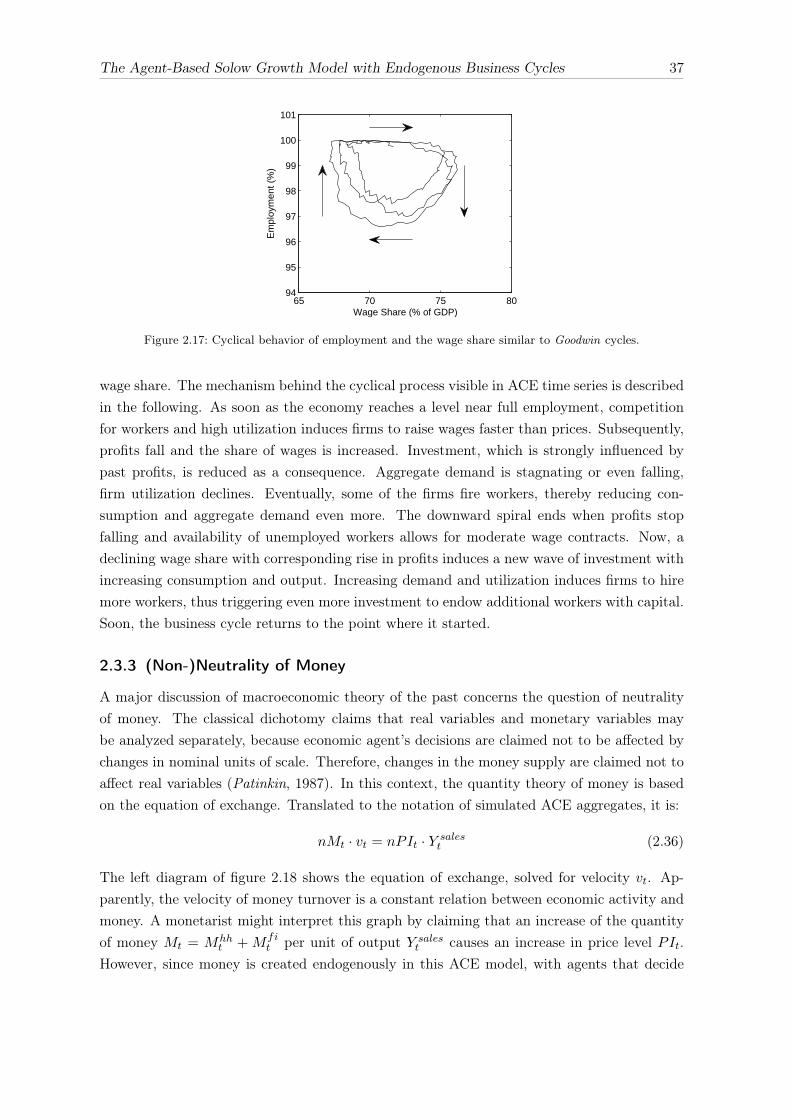
The Agent-Based Solow Growth Model with Endogenous Business Cycles 37
65 70 75 8094
95
96
97
98
99
100
101
Em
ploy
men
t (%
)
Wage Share (% of GDP)
Figure 2.17: Cyclical behavior of employment and the wage share similar to Goodwin cycles.
wage share. The mechanism behind the cyclical process visible in ACE time series is describedin the following. As soon as the economy reaches a level near full employment, competitionfor workers and high utilization induces firms to raise wages faster than prices. Subsequently,profits fall and the share of wages is increased. Investment, which is strongly influenced bypast profits, is reduced as a consequence. Aggregate demand is stagnating or even falling,firm utilization declines. Eventually, some of the firms fire workers, thereby reducing con-sumption and aggregate demand even more. The downward spiral ends when profits stopfalling and availability of unemployed workers allows for moderate wage contracts. Now, adeclining wage share with corresponding rise in profits induces a new wave of investment withincreasing consumption and output. Increasing demand and utilization induces firms to hiremore workers, thus triggering even more investment to endow additional workers with capital.Soon, the business cycle returns to the point where it started.
2.3.3 (Non-)Neutrality of Money
A major discussion of macroeconomic theory of the past concerns the question of neutralityof money. The classical dichotomy claims that real variables and monetary variables maybe analyzed separately, because economic agent’s decisions are claimed not to be affected bychanges in nominal units of scale. Therefore, changes in the money supply are claimed not toaffect real variables (Patinkin, 1987). In this context, the quantity theory of money is basedon the equation of exchange. Translated to the notation of simulated ACE aggregates, it is:
nMt · vt = nPIt · Y salest (2.36)
The left diagram of figure 2.18 shows the equation of exchange, solved for velocity vt. Ap-parently, the velocity of money turnover is a constant relation between economic activity andmoney. A monetarist might interpret this graph by claiming that an increase of the quantityof money Mt = Mhh
t + Mfit per unit of output Y sales
t causes an increase in price level PIt.However, since money is created endogenously in this ACE model, with agents that decide

The Agent-Based Solow Growth Model with Endogenous Business Cycles 38
freely about the desired amount of transaction money, such an interpretation is invalid. Ac-tually, agents hold transaction money as high as previous month’s individual cost, plus aliquidity buffer of 20%. As a result, velocity of monthly money holding is slightly higher than1, when compared to monthly turnover. Causality runs from price level to the desired andrealized amount of transaction money, not vice versa.Economists in the tradition of Keynes argue that money actually affects economic activity.
Recent New Keynesian DSGE models incorporate frictions of price and wage developmentsthat render short-run economic activity influenceable by monetary policy., However, in thelong run, the classical dichotomy holds (see, for example, Benchimol and Fourçans, 2012).The New Keynesian Phillips curve marks the short run efficiency of monetary policy.
0 5 10 15 200
0.5
1
1.5
2
v =
M /
(P⋅ Y
)
Years0 1 2 3 4
0.5
1
1.5
2
2.5
Unemployment (%)
Infla
tion
(%)
Figure 2.18: Left: Velocity of money turnover, Right: Phillips curve at π∗ = 1.2% of 240 subsequent monthlyobservations. Dashed line depicts OLS regression.
The presented ACE model also generates a Phillips curve relationship, which will be derivedhere: Inflation is measured as a growth rate of the price index PIt, which itself depends onprice decisions of each single firm (cf. equations (2.11), (2.12) and (2.16) above). Now, firmprices are driven by a common value for expected inflation πet , therefore aggregate inflationis also directly influenced by it. Moreover, firms accelerate or slow down their individualtarget price development with capacity utilization. On aggregate, there is a continuum offirm capacity utilization levels. As the right diagram of figure 2.11 indicates, the positioningof this continuum shifts with aggregate capacity utilization Ut:
Ut =
∑Nfi
i=1 YSalest,i∑Nfi
i=1 Yct,i
(2.37)
If Ut increases (decreases), a larger number of firms faces high (low) levels of capacity uti-lization, thus inflation accelerates (slows down). On aggregate, we can state that inflation isdriven by aggregate utilization, or rather its deviation from target:
πt ≈ πet + f (Ut − U∗) (2.38)
Please note the similarity to a New Keynesian Phillips curve (Woodford, 2003), except thatthe output gap has been replaced by a “utilization gap” as another measure for aggregate

The Agent-Based Solow Growth Model with Endogenous Business Cycles 39
economic activity. Another difference is that inflation expectation πet is purely adaptive,so there is no rational expectations hypothesis employed. Moreover, no stochastic term isexplicitly given, although there are stochastic elements incorporated in the ACE simulation,for example the number of firms that actually adjusts its price in a certain month.In the ACE economy, a Phillips curve is clearly visible in the right diagram of figure 2.18,
where annual inflation is plotted against current unemployment, indicating non-neutrality ofmoney at least in the short run. Due to adaptive expectations, a central bank that tries toreduce unemployment by increasing its inflation target will increase demand in the short run.However, there is no trade-off in a way that higher inflation causes low unemployment, as wasimplicitly assumed in the “rules vs. discretion” debate.25
0 5 10 15 200
0.5
1
1.5
2
2.5
3
3.5
Infla
tion
(%)
0 5 10 15 2095
96
97
98
99
100
Em
ploy
men
t (%
)
0 1 2 3 4
1
1.5
2
2.5
3
Unemployment (%)In
flatio
n (%
)
Figure 2.19: Adjustment after shock to inflation target from 1.2% to 1.8%. Left: Inflation, Middle: Employ-ment, Right: Phillips curve 240 monthly observations right after shock month.
The direction of causality runs strictly from economic activity to rising prices in this model.Nevertheless, monetary policy is not necessarily inefficient: A sudden increase of the inflationtarget induces monetary policy to lower the nominal interest rate, which moves economicactivity upward in the short run. Adaptive expectations subsequently adjust to the new levelof inflation and afterwards, the central bank faces a shifted Phillips curve that emerges from ahigher inflation target. See Figure 2.19 to see the adjustment process after the annual inflationtarget is increased to π∗ = 1.8% at year 5. Inflation almost immediately switches to cyclicalfluctuation on a higher average level of inflation. Employment also continues in its cyclicalpattern. The graph on the right side depicts the Phillips curve relationship for 240 monthlyobservations after the shock month. Clearly, the new Philips curve relation is simply shiftedupward. Therefore, monetary policy is neutral with respect to real variables in the mediumand long run.
25See Kydland and Prescott (1982). According to this view, a representative agent balances leisure and consump-tion. Surprise inflation, in turn, induces the agent to work more, as a result of erroneously over-estimatingthe real purchasing power of nominal wages. This is a good example for the limited explanatory value ofmicrofoundations, if assumptions on individual behavior are questionable. In the real world, most householdsdetermine their level of work time by a mixture of labor contracts with fixed hours (as a convention of soci-ety) and the need to satisfy their employer, who might ask for temporary overtime to accommodate demandvariations.

The Agent-Based Solow Growth Model with Endogenous Business Cycles 40
2.3.4 Stabilization policy
The tax regime of “automatic stabilization” as described above (section 2.2.5, equation (2.29))is applied in all diagrams throughout this article, except partly for this section. Its mecha-nism is shown in the left side of figure 2.20. The upper graph shows public cost and revenue;the corresponding tax rate is depicted in the middle and the bottom graph depicts aggregateemployment. Please note that the tax rate remains stable slightly above 9%. In recessions,tax revenue is stagnating, while public cost for unemployment benefits is increasing strongly.Therefore, the fiscal deficit is increasing during economic downturn, so that we have an effectof automatic stabilization of aggregate demand: Public debt growth is increased in timesof recession.26 Fluctuations of demand are dampened automatically by the state, which isthe reason for the term “Automatic Stabilization” assigned to this tax regime. A second tax
0 5 10 15 206
7
8
9
10
11
x 106
Cos
t & R
even
ue
0 5 10 15 20
8
10
12
14
Tax
Rat
e (%
)
0 5 10 15 2092
94
96
98
100
Em
ploy
men
t (%
)
Years
0 5 10 15 20
6
7
8
9
10
x 106
Cos
t & R
even
ue
0 5 10 15 20
8
10
12
14
Tax
Rat
e (%
)
0 5 10 15 2092
94
96
98
100
Em
ploy
men
t (%
)
Years
0 5 10 15 20
6
8
10
12
x 106
Cos
t & R
even
ue
0 5 10 15 20
8
10
12
14
Tax
Rat
e (%
)
0 5 10 15 2092
94
96
98
100
Em
ploy
men
t (%
)
Years
Figure 2.20: Fiscal Policy Regimes: Automatic Stabilization (left side), Deficit Spending (middle) and Pro-Cyclical (right). All columns show: Upper diagram: Public cost (dotted) and revenue (solid), middle: Taxrate, bottom: Employment.
regime is termed “Deficit Spending”, which is shown in the middle column of figure 2.20. Sincethis is a Keynesian model characterized by demand-led economic activity, it is not surprisingthat fiscal policy aiming at demand stabilization actually works. The government in this ACE
26Public debt varies between 15 and 20% of the capital stock value in the presented setting. When comparedto annual turnover, the public debt burden is stable at 25-35% of GDP.

The Agent-Based Solow Growth Model with Endogenous Business Cycles 41
model does not directly buy goods and services. Instead, aggregate demand is influenced byadjusting the general income tax. Whenever aggregate utilization falls considerably belowtarget, the state reacts with a tax cut in order to stimulate consumption expenditure. Oth-erwise, the tax rate is adjusted according to the regime of “Automatic Stabilization”, definedas τt in equation (2.29). The deficit-spending tax rate is adjusted according to
τDeft =
τt if Ut − U∗ ≥ −0.01
τt + (Ut − U∗) if Ut − U∗ < −0.01(2.39)
The second column of diagrams in figure 2.20 depicts the fiscal regime of deficit spending.As the employment plot (bottom diagram) shows, business cycles are dampened considerablyin this Keynesian regime of demand stabilization. As a result, there is less unemployment onaverage, so that financing requirements of the general income tax are even reduced. Therefore,the average tax rate is slightly lower at approximately 8.5−9%. Public debt is also lower in thisregime, because high deficits in times of recession are reduced in frequency and magnitude.27
In principle, the ACE framework allows for stabilization of aggregate demand with a higheraverage level of output. In General Equilibrium frameworks such as Lucas (2003) as wellas Gali, Gertler and López-Salido (2007), deviations from potential output are symmetricand can only be dampened in both directions. However, the modeled stabilization policy ofdeficit spending shows how it becomes possible in ACE models to “fill in troughs withoutshaving off peaks” (DeLong and Summers, 1988, p. 434). The employment plot in themiddle column of figure 2.20 shows the reduction of unemployment in recessions and onaverage. Therefore, stabilization policy in an ACE framework offers additional welfare gainscompared to General Equilibrium models as applied by Lucas (2003). Risk-averse individualswill not only appreciate reduced variability of consumption and employment, they will captureadditional welfare gains from a higher level of average consumption.28
Finally, a third tax regime is termed “pro-cyclical”, which is shown in the right column offigure 2.20. Again, the government conducts fiscal policy in this ACE model by adjustingthe general income tax. Here, the state aims at balancing of public finance requirements andcollected taxes permanently throughout business cycles. To this end, a recession, which isaccompanied by a stagnating tax base and rising cost, is answered with an increasing tax rate,thereby dampening aggregate consumption even more. The respective tax rate is given by:
τProt = 0.95 · UPt−1 · nUBt−1 + Lst · nWIt−1 − it · nSCstt − nSGt−1
nInct−1(2.40)
27Public debt in the deficit spending regime varies between 7 and 11% of the capital stock value, given thesame model parametrization. When compared to annual turnover, the debt burden is stable at 15-20% ofGDP. That is, public debt is considerably lower than in the benchmark regime of automatic stabilization.Compared to real-world experience with Keynesian fiscal policy in the twentieth century, this result appearscounter-factual.
28Moreover, we might determine additional gains from analyzing welfare on disaggregate level. Income and con-sumption paths of individual heterogeneous agents are considerably less volatile, because a smaller proportionof agents becomes unemployed at all. Therefore, welfare gains of stabilization are even higher.

The Agent-Based Solow Growth Model with Endogenous Business Cycles 42
Observe the parallel development of cost and revenue in the upper diagram of the rightcolumn of figure 2.20, thus indicating a stable budget deficit as was intended by this policyregime. However, the tax rate is increased pro-cyclically whenever demand and utilization islow already, thus dampening consumption even more. In the other extreme, the tax rate islowered when the economy is at full employment levels and aggregate demand is at its peak,thus stimulating economic activity even more. As a result, business cycles are reinforced andamplified, with considerably higher unemployment burdens and longer duration. Therefore,fiscal policy aiming at permanently balancing the state deficit is accompanied by high cost tosociety.29
Keynes (1936) showed that anti-cyclical fiscal policy is effective when the goal is to dampenrecessions. It should have become public knowledge by now that pro-cyclical fiscal policy willhave strongly adverse effects on the real economy, as shown in former analysis. However, in thecurrent Euro crisis, economic policy of austerity is forced on southern Euro-zone countries.When investment activity and aggregate demand in general are low already, accompaniedby lower tax revenue and increasing cost, governments in these countries are “encouraged”to balance the budget pro-cyclically. As a result, southern Euro-zone countries face highunemployment rates and deflationary tendencies.30 In a system of double-entry bookkeeping,it can be shown that it is not possible to reduce public debt and firm sector debt at the sametime, if there is no other group of agents which is willing to spend considerably more.31
2.3.5 Calibration
The model is calibrated to produce a number of desired properties and proportions on aggre-gate level. Business cycles are of 7 years frequency, which corresponds quite well to Juglarcycles with a length between 7 and 11 years as reported by Korotayev and Tsirel (2010).However, in the absence of exogenous shocks in the simulation, endogenous simulated cyclesare more predictable and more even, when compared to real-world business cycle occurrences.
Figure 2.21 (again) depicts real values for production capacity (dotted line), firm sales(solid) and consumption (dashed) per capita (as shown before). Please note the upwardtrend of shown measures. Even production capacity fluctuates around a trend, since firmsreduce employment and capital accumulation during recessions. Note that consumption isconsiderably less volatile than investment, given as distance between sales and consumption,which is in line with stylized facts (cf. Stock and Watson, 1999). The annual growth rate ofaggregate firm sales (real GDP) varies approximately between −1.5% in economic downturnand +3.5% in times of boom. All real variables grow annually at 1.2% in the long run. Over
29Public debt in the pro-cyclical regime varies between 8 and 9% of the capital stock value, given the samemodel parametrization. When compared to annual turnover, the debt burden is stable at 15-20% of GDP.
30At this point, it is still unclear whether the strategy will at least accomplish the goal of an internal devaluationof countries in a crisis of competitiveness in the end. The future will show whether imbalances within theEuro zone can be reduced sufficiently, before pro-cyclical policy is perceived too costly to society.
31See proof in appendix 2.B.

The Agent-Based Solow Growth Model with Endogenous Business Cycles 43
0 5 10 15 20
2500
3000
3500
4000
Con
sum
ptio
n, S
ales
, Cap
acity
p.c
.
Years
Figure 2.21: Per capita real production capacity (dotted line), real firm sales (solid) and real consumption(dashed).
20 years, exponential growth of 0.1% per month amounts to an increase of 27.1%.The annual depreciation rate of productive firm capital is set at 9.6%. Madsen et al.
(2012) distinguish average depreciation rates of firm capital into structures (buildings) with adepreciation rate of 1.75% and machinery and equipment with a depreciation rate of 17.6%.So the chosen depreciation rate is a compromise between both components of firms capitalstocks. Chiarella, Flaschel and Franke (2005, p. 85) refer to detailed data on the US economyand calculate with a similar capital depreciation rate (9.5%) as this model. The ACE modelproduces a capital-output ratio of approximately 185%. This amounts to a reciprocal valueof output to firm capital Y/K of 0.54 and is a reasonable order of magnitude for developedeconomies. Madsen et al. (2012) estimate a long-run average for 16 OECD countries for Y/Kand find it to converge to levels of about 0.5 since 1980. Chiarella et al. (2005, p.85) calculatewith 0.7 for the Y/K ratio referring to US data.A wage share of approximately 70−75% is slightly higher than respective proportions in real-
world developed economies. According to OECD data (stats.oecd.org) for the total economyin Germany and the US, the wage share ranged between 65% and 70% recently. However,unlike the simulated economy, in real world economies there are considerable amounts ofcapital in the form of real estate: returns of invested capital in real estate also contributeto overall GDP. Closely related, the average profit rate of simulated firms ranges between5% in recessions and 8% in booms, so we have an average return rate to invested capital ofapproximately 6 − 7%. The average return rate to (debt-free) equity is considerably higherat 10− 12%.32
Finally, figure 2.22 depicts the correlation between detrended GDP and price level for 24months backward and forward. For comparison, respective lags (on a quarterly basis) forUS data between 1947 and 2007 are shown as reported by Lengnick (2013). Apparently, thepattern is rather similar, so the model qualitatively fits real data quite well.
32The implied distribution of simulated GDP (100%): Wages (70-75%), Depreciation (17-18%), Profit (9-15%).Multiplying profit (as percentage of GDP) by simulated output-capital ratio (Y/K = 0.54) yields a profit rateranging between 5 and 8 per cent again.

The Agent-Based Solow Growth Model with Endogenous Business Cycles 44
−8 −6 −4 −2 0 2 4 6 8−1
−0.5
0
0.5
Lags (quarters)
Cor
rela
tion
GD
P a
nd la
gged
PI
modelUS 1947Q1−2007Q3
Figure 2.22: Correlation of detrended GDP and detrended Price Index from ACE model (solid line) and withdata for the US economy between 1947 and 2007 (dotted line).
2.3.6 Limitations and Parameter Sensitivity
Since the developed model does not perfectly mimic real-world behavior on individual level,consider this (not necessarily exhaustive) list of limitations: Concerning firms, (1) competitionbetween them is reduced to price competition (for customers) and wage competition (foremployees), which does not even closely capture the complexity of actual firm decisions. Toname a few, innovation, marketing, product quality and corporate governance are left out. (2)The model abstracts from firm entry and exit. (3) The firm size distribution as depicted inFigure 2.23 is skewed to the right, which is a stylized fact (Delli Gatti et al., 2010). However,the range of firm sizes is very limited. Realism in this respect is beyond the scope of thisarticle. (4) Firms are behaving according to fixed rules instead of adapting their strategiesin a process of learning. (5) Technological progress is exogenous instead of being the productof innovative activities; a criticism that also applies to the Solow model, which induced morerecent developments of modern growth theory.
0 10 20 30 40 500
500
1000
1500
2000
2500
Employment
Fre
quen
cy
0 5 10 15
x 104
0
500
1000
1500
2000
Detrended Sales
Fre
quen
cy
Figure 2.23: Distributions of monthly firm size (100 firms, 20 years): Employees (left) and detrended sales(right).
Workers, on the other hand, (1) are modeled with identical labor supply, so there areno individual differences in capabilities, human capital, specialization or productivity. (2)Household agents are infinitely living. (3) The distribution of firm shares is fixed from thebeginning, so there is no market to trade shares and no market determining asset prices. (4)

The Agent-Based Solow Growth Model with Endogenous Business Cycles 45
Savings and asset prices are not subject to agent behavior, for example asset prices inflationmight increase household consumption. (5) ACE modeling permits investigation of topicsrelated to wealth and income distribution. However, the current model specification is notcalibrated with respect to actual distributions.Lorenz (1905) curves are depicted in figure 2.24, which are useful to visualize the concen-
tration of wealth (left) and income (right) in the population. It was measured at the end ofthe period presented throughout the diagrams above. Starting from an initially equal wealthdistribution, even after more than 100 years wealth inequality did not increase to extremelevels. Moreover, the income distribution is almost egalitarian. The reason is that householdsare modeled homogeneous with respect to the value of individual labor supply, which renderswages between households almost identical. Since about 80% of national income consist ofwages, the income distribution would be quite close to equality, even if the wealth distributionreflected a maximum level of inequality. Moreover, the modeled income tax applies equallyto all levels of wage and capital income. It appears to be a fruitful area of future research toapply realistic patterns for a wealth and income distribution.
0 50 1000
20
40
60
80
100
% o
f Wea
lth
% of Population0 50 100
0
20
40
60
80
100
% o
f Inc
ome
% of Population
Figure 2.24: Lorenz curve of wealth (left) and income distribution (right).
Regarding sensitivity of model parameters, it should be distinguished between two differentgoals: Stability and establishment of business cycles. First, in order to render the simulatedeconomy somewhat stable, hyper inflation or a deflationary depression with increasing debtburdens should be avoided. To this end, some parameters are crucial: (1) Model parameters ofthe consumption function have to be chosen, so that the sum of consumption and investmentis sufficiently utilizing firm capacities. Aggregate demand needs to be in a range that allowsthe central bank to stabilize aggregate demand at a level, that corresponds to firms’ targetcapacity utilization. (2) Another important parameter is λπ, which allows the central bank todirectly influence expected inflation. In the current setting it is 0.1, however, if it is 0, adaptiveinflation expectations become much more likely to destabilize the economy in a deflationaryor inflationary spiral. (3) Upper and lower boundaries for acceptable firm utilization levelsshould not be too narrow. Otherwise, employment becomes volatile with small variations inaggregate demand. This becomes critical, when fired workers reduce consumption, so thataggregate demand is lowered even more, thus triggering firing decisions of other firms. (4)

The Agent-Based Solow Growth Model with Endogenous Business Cycles 46
Limited variability of firm investment is a desired property, but it should also remain reliablystable. If, for example, a firm tried to invest as much to directly “jump” to the target capitalstock in a single month, aggregate investment might become extremely volatile. In thatsituation, firms might suddenly be unable to satisfy demand on aggregate scale, rendering thecentral bank unable to influence aggregate output sufficiently.Secondly, the establishment of a business cycle pattern as presented in this article is quite
sensible to model parameters determining firm investment. Small variations may influencethe shape and intensity of endogenously created business cycles strongly, with the possibleresult, that variability vanishes almost completely. Among the most important parametersfor emergence of business cycles are: (1) Parameter a∆h which determines the dependence ofinvestment on changes in profits is particularly critical. (2) Parameter ah which determinesthe degree to which investment is influenced by past profits. (3) The depreciation rate, whichdetermines the level of gross investment as a major component of aggregate demand. (4) Thefrequency of business cycles is strongly affected by investment inertia λI . However, seeminglyunrelated parameters in their interplay may also influence the pattern to some extent. Thepresented set of parameter values was determined in a process of trial and error by usingcommon-sensical reasoning. It is a characteristic feature of agent-based computational modelswith a considerable degree of complexity, that aggregate dynamic model behavior can not betraced back to a single parameter. Therefore, it is a feature of ACE models that can hardlybe displaced.
2.4 Conclusion
“Yet another model” might be a comprehensible first comment on a newly developed macromodel. There have been numerous attempts to establish new models and new variants ofexisting models. These models differ with respect to the underlying paradigm, thus high-lighting different mechanisms or key variables. Surely it constitutes a sound request to askwhether a new model actually contributes to this large reservoir of ideas and elaborate modelconstructions.First, agent-based computational economics is a fairly new and yet densely populated field
of research, compared to widespread paradigms like general equilibrium models. The merenumber of economists employing this way of model-building is limited, so chances are thatyet undiscovered ideas emerge when conducting research off the beaten track. Secondly, thepresented model combines modeling of economic growth and business cycle dynamics in acomprehensive approach, where even unemployment is modeled explicitly, instead of simplyrelying on the link of output and employment. Usually, growth and business cycle dynam-ics are analyzed separately, although they are related closely. Thirdly, the newly presentedmodel is capable of incorporating elements and ideas from different perspectives and economicschools. It encompasses neoclassical technology and investment decisions; Keynesian ideasenter in multiple ways such as demand-led output determination, involuntary unemployment,income-dependent consumption and business cycles, that are created and reinforced by in-

The Agent-Based Solow Growth Model with Endogenous Business Cycles 47
vestment activity as the main engine of market economies. Monetary policy is conducted inaccordance with the Taylor rule. Moreover, it is designed as a monetary model with double-entry bookkeeping, allowing for close supervision of monetary flows between agents and groupsof agents.The model simulates households and firms as artificial objects in a computer simulation,
who interact according to behavioral rules on a goods market and on a labor market. A stateprovides for unemployment benefits and collects taxes, a central bank adjusts the nominalinterest rate in order to stabilize inflation close to a target level. Firm investment is modeledsuch that it is reinforced by rising profit, whereas firm profit in turn depends on aggregateinvestment activity. This way, a virtuous circle (or a vicious circle) in the interplay of in-vestment and profit generates recurrent waves of increasing and declining economic activityon aggregate level. Business cycles are created endogenously from investment activity, whosefluctuations are transmitted to firm demand, capacity utilization, employment and price set-ting behavior. Model parameters are calibrated in order to mimic reasonable macroeconomicproportions like cycle length, the capital-output ratio and the wage share.As it turns out, the model is capable to generate Goodwin cycles and a Phillips curve
relationship. After a monetary policy shock with a higher inflation target, the Phillips curveis simply shifted upward, so money neutrality holds in the long run. Demand stabilizationpolicy is shown to dampen business cycles considerably, while on the contrary, a pro-cyclicalfiscal regime is characterized by business cycles of larger amplitude and cycle length.In addition, it appeals to common-sense, when modeled firm agents resemble important
characteristics of real-world firms. Decisions are constructed to actually depend on the amountof goods or services, that a firm is able to sell. This explicit demand-led property of firmbehavior is absent in many other models. As a consequence, production decisions are generallynot limited by restricted availability of resources or rising marginal cost of production, whichis counter-factually assumed in many models (e.g. Lindbeck and Snower, 1994). Instead,modeled firms are restricted by demand and would be glad to sell as many units as possible.As Sraffa (1926) puts it: “The chief obstacle against which [business men] have to contendwhen they want gradually to increase their production does not lie in the cost of production– which, indeed, generally favors them in that direction – but of the difficulty of selling thelarger quantity of goods without reducing the price [...]”Avenues for future research are plenty in the yet densely populated world of ACE modeling.
For example, starting from this presented model, imposing a more realistic distribution ofincome and wealth among households would be required to investigate suppositions aboutrelationships of certain macro variables with measures of wealth concentration. Anotherexample would be the design of herd behavior among firms concerning economic outlook,combined with firm investment depending on this level of sentiment. Waves of high and loweconomic sentiment index values might thus be transmitted to real variables, so that businesscycles emerge from a process of social opinion formation (Lux and Stolzenburg, 2011).

The Agent-Based Solow Growth Model with Endogenous Business Cycles 48
2.5 Bibliography
[1] Ackerman, F. (2002). Still dead after all these years: interpreting the failure of generalequilibrium theory. Journal of Economic Methodology 9(2), 119–139.
[2] Alesina, A., Rodrick, D. (1994). Distributive Politics and Economic Growth. QuarterlyJournal of Economics 109(2), 465–90.
[3] Barro, R.J., Sala-i-Martin, X. (2003). Economic Growth. MIT Press, ed.2, vol.1.
[4] Blinder, A. (1999), Central Banking in Theory and Practice. MIT Press Cambridge.
[5] Calvo, G.A., 1983. Staggered prices in a utility-maximizing framework, Journal of Mon-etary Economics, No. 12(3), pp. 383–398.
[6] Chiarella, C., Flaschel, P., Franke, R. (2011). Foundations for a Disequilibrium Theoryof the Business Cycle. Cambridge University Press.
[7] Clarida, R., Gali, J., Gertler, M. (1999). The Science of Monetary Policy: A New Key-nesian Perspective. Journal of Economic Literature 37(2), 1661–1707.
[8] Colander, D., Föllmer, H., Haas, A., Goldberg, M., Juselius, K., Kirman, A., Lux, T.,Sloth, B. (2009). The financial crisis and the systemic failure of the economics profession.Critical Review 21(2–3), 249–267.
[9] De Long, J.B., Summers, L.H. (1988). Brookings Papers on Economic Activity 19(2),433–494.
[10] Delli Gatti, D., Gaffeo, E., Gallegati, M. (2010). Complex agent-based macroeconomics:a manifesto for a new paradigm. Journal of Economic Interaction and Coordination 5(2),111–135.
[11] Dobb, M. (1973). Theories of value and distribution since Adam Smith. Cambridge Uni-versity Press.
[12] Dosi, G., Fagiolo, G., Roventini, A. (2008). The microfoundations of business cycles: anevolutionary, multi-agent model. Journal of Evolutionary Economics 18, 413–432.
[13] Dynan, K.E. Skinner, J. and Zeldes, S.P. (2004). Do the Rich Save More? Journal ofPolitical Economy 112(2), 397–444.
[14] Benchimol, J., Fourçans, A. (2012). Money and risk in a DSGE framework: A Bayesianapplication to the Eurozone. Journal of Macroeconomics 34, 95–111.
[15] Gaffeo, E., Delli Gatti, D., Desiderio, S., Gallegati, M. (2008). Adaptive microfoundationsfor emergent macroeconomics. Eastern Economic Journal 34 (4), pp. 441–463.

The Agent-Based Solow Growth Model with Endogenous Business Cycles 49
[16] Galí, J., Gertler, M., López-Salido, J.D. (2007). Markups, Gaps, and the Welfare Costsof Business Fluctuations. Review of Economics and Statistics 89(1), 44–59.
[17] Galor, O. (2009). Inequality and Economic Development. Edward Elgar Publishing Lim-ited, Cheltenham.
[18] Goodwin, R.M. (1967). A Growth Cycle, in C.H. Feinstein (edt.): Socialism, Capitalismand Economic Growth. Cambridge.
[19] Hein, E., Schoder, C. (2011). Interest rates, distribution and capital accumulation – Apost- Kaleckian perspective on the US and Germany. International Review of AppliedEconomics 25(6), 693–723.
[20] Kalecki, M. (1937). A Theory of the Business Cycle, Review of Economic Studies 4, 77–97. Reprinted in: Kalecki, M. (1971), Selected Essays on the Dynamics of the CapitalistEconomy. 1933-1970. Cambridge University Press.
[21] Keynes, J.M. (1936). The General Theory of Employment, Interest and Money, London(reprinted 2007).
[22] Kirman, A.P. (1992). Whom or what does the representative individual represent? Jour-nal of Economic Perspectives 6(2), pp. 117–136.
[23] Kirman, A.P. (2006). Demand theory and general equilibrium: from explanation to in-trospection, a journey down the wrong road. History of Political Economy 38, 246–280.
[24] Korotayev, Andrey V., Tsirel, Sergey V. (2010). A Spectral Analysis of World GDPDynamics: Kondratieff Waves, Kuznets Swings, Juglar and Kitchin Cycles in GlobalEconomic Development, and the 2008–2009 Economic Crisis. Structure and Dynamics4(1), 3–57.
[25] Kydland, F., and E. C. Prescott (1977). Rules Rather than Discretion: The Inconsistencyof Optimal Plans. Journal of Political Economy, 473–492.
[26] Lengnick, M. (2013). Agent-based macroeconomics: A baseline model. Journal of Eco-nomic Behavior and Organization 86, pp. 102–120.
[27] Lindbeck, A., Snower, D.J. (1993). How are Product Demand Changes Transmitted tothe Labor Market? Economic Journal 104 (423), 386–398.
[28] Lorenz, M.O. (1905). Methods of measuring the concentration of wealth. Publications ofthe American Statistical Association 9(70), 209–219.
[29] Lucas, R. (1976). Econometric Policy Evaluation: A Critique. In: Brunner, K.; Meltzer,A. (edt.) The Phillips Curve and Labor Markets. Carnegie-Rochester Conference Serieson Public Policy 1, 19–46.

The Agent-Based Solow Growth Model with Endogenous Business Cycles 50
[30] Lucas, Jr., R.E. (2003). Macroeconomic priorities, American Economic Review 93(1),1–14.
[31] Lux, T., Stolzenburg, U. (2011). Identification of a Core-Periphery Structure AmongParticipants of a Business Climate Survey. European Physical Journal B 84, 521–533.
[32] Madsen, J.B., Mishra, V. and Smyth, R. (2012). Is the Output-Capital Ratio Constantin the Very Long Run? The Manchester School 80(2), pp. 210–236.
[33] Mankiw, N.G. (2000). Makroökonomik. 4th edt., Schäffer-Poeschel, Stuttgart.
[34] Mankiw, N.G. (2006), The Macroeconomist as Scientist and Engineer, Journal of Eco-nomic Perspectives 20(4), 29–46.
[35] Oeffner, M., (2008). Agent-Based Keynesian Macroeconomics - An Evolutionary ModelEmbedded in an Agent-Based Computer Simulation, MPRA Paper 18199, UniversityLibrary of Munich.
[36] Page, S.E. (2008). "Agent-based models," The New Palgrave Dictionary of Economics,2nd Edition.
Patinkin, D. (1987). Neutrality of money, The New Palgrave: A Dictionary of Economicsv.3, 639–644.
[37] Solow, R.M. (1956), A contribution to the Theory of Economic Growth, Quarterly Jour-nal of Economics 70, 5–94.
[38] Solow, R. (2010). Building a Science of Economics for the Real World.Prepared Statement of Robert Solow, Professor Emeritus, MIT, to theHouse Committee on Science and Technology, Subcommittee on Investiga-tions and Oversight: July 20, 2010. Link: http://www2.econ.iastate.edu/classes/econ502/tesfatsion/Solow.StateOfMacro.CongressionalTestimony.July2010.pdf
[39] Schelling, T.C. (1969). Models of segregation. American Economic Review 59(2), 488–493.
[40] Sims, C.A., (1980). Macroeconomics and reality. Econometrica 48, 1–48.
[41] Sraffa, P. (1926). The Law of Returns Under Competitive Conditions. Economic Journal40, S.538–550.
[42] Stock, J., Watson, M. (1999). Business cycle fluctuations in U.S. macroeconomic time se-ries. In: Taylor, J., Woodford, M. (eds.). Handbook of macroeconomics. Elsevier Science,Amsterdam.
[43] Swan, T.W. (1956). Economic Growth and Capital Accumulation. Economic Record 32(2): 334–361.

The Agent-Based Solow Growth Model with Endogenous Business Cycles 51
[44] Syll, L.P. (2012). Rational expectations - a fallacious foundation for macroeconomics ina non-ergodic world. real-world economics review 62, 34–50.
[45] Taylor, J.B. (1993). Discretion versus Policy Rules in Practice. Carnegie-Rochester Con-ference Series on Public Policy 39, 195–214.
[46] Tesfatsion, L. (2003). Agent-based Computational Economics: Modeling Economies asComplex Adaptive Systems. Information Sciences 149(4), 262–268.
[47] Woodford, M. (2003). Interest and prices: Foundations of a theory of monetary policy.Princeton, New Jersey: Princeton University Press.

The Agent-Based Solow Growth Model with Endogenous Business Cycles 52
2.A Appendix: List of Symbols and Model Parameters
Symbol Type Unit/Value Descriptioni subscript # Firm numberh subscript # Household numbert subscript # Monthah Parameter 7 Dependence of firm investment on profit ratea∆h Parameter 5 Dependence of firm investment on change in profit rateau Parameter 0.03 Dependence of firm wage setting on utilizationam Parameter 0.05 Dependence of firm wage setting on price markupα Parameter 0.2 Cobb-Douglas capital exponentc Parameter 0.85 Marginal rate of consumptiongA Parameter (annually) 1.2% Technology growth rateγp Parameter 5 Price competition intensityγr Parameter 0.5 Restriction aversionγw Parameter 2.5 Wage competition intensityλI Parameter 0.9 Investment inertiaλC Parameter 0.9 Consumption inertiaLst Parameter 200 Public Employment (fixed)m∗ Parameter 60% Target price markup over unit wage costNhh Parameter 2,000 Number of householdsNfi Parameter 100 Number of firmspp Parameter 25% Probability to search for a cheaper supplying firmpr Parameter 25% Probability to reconsider 1 connection to restricting firm(s)ps Parameter 2% Probability to replace 1 connection randomlyπ∗ Parameter (annually) 1.2% Inflation targetρ Parameter (annually) 9.6% Capital stock depreciation rateσp Parameter 0.14 Standard deviation of bell curve (price setting behavior)T Parameter 3,000 Number of simulated monthsTπ Parameter 24 Backward-looking months of adaptive inflation expectationTu Parameter 6 Backward-looking months of short run utilization averageTw Parameter 6 Backward-looking months of employment target fulfillmentU∗ Parameter 85% Firm target utilizationU∗ Parameter 78% Firm lower bound utilizationU∗ Parameter 91% Firm upper bound utilization
At Variable real number Technology parameter (growing)Ct Variable goods Aggregate real consumptionCt,h Variable goods Real household consumptionCt Variable goods Autonomous real household consumptiondur Variable # Wage contract duration (month number)DPt,i Variable ∈ {−1, 0, 1} Decision target price change (Price setting behavior)DWt,i Variable ∈ {−1, 0, 1} Decision target wage change (Wage setting behavior)εp RV ∈ (0, 0.015) Stochastic price changeεw RV ∈ (0, 0.01) Stochastic wage changeit Variable % Nominal interest rateIt Variable goods Aggregate real gross investmentIt,i Variable goods Firm real gross investmentInett−1,i Variable goods Firm real net investmentKt,i Variable goods Firm real capital stock
Continued on next page

The Agent-Based Solow Growth Model with Endogenous Business Cycles 53
Table – ContinuedSymbol Type Unit/Value DescriptionK∗t,i Variable goods Firm target capital stockLt,i Variable # Firm employeesL∗t,i Variable # Firm employment targetmt,i Variable % Firm markup over unit wage costν RV ∈ {0, 1, .., 4} Stochastic wage contract duration (+10)πt Variable % Inflation rate during last 12 monthsπet Variable % Expected inflation rateπmt Variable % Monthly inflation rate (annualized)rt Variable % Expected real interest rater∗ Variable % Long run real interest rateRNIt,h Variable goods Real net disposable household incomeRoCt,i Variable % Profit rate (Return on capital stock)RoC
12t,i Variable % Profit rate (RoC) during last 12 months
RoEt,i Variable % Return on equityτt Variable % Tax rate in default fiscal policy regime “Automatic Stabil.”τDeft Variable % Tax rate in fiscal policy regime “Deficit spending”τProt Variable % Tax rate in fiscal policy regime “Pro-cyclical”Ut,i Variable % Firm utilizationUt Variable % Aggregate utilizationUPt Variable # Unemployed personsY ct,i Variable goods Firm real production capacityY salest,i Variable goods Firm real salesY salest Variable goods Firm turnover / Aggregate salesnCt,h Variable currency Nominal household consumption expenditurenFSt Variable currency Fiscal surplus / deficitnIt,i Variable currency Firm nominal investment expenditurenIncprimt,h Variable currency Primary household incomenIncnett,h Variable currency Net household income (secondary)nMt Variable currency Aggregate transaction moneynMhh
t Variable currency Aggregate household sector moneynMhh
t,h Variable currency Household moneynMfi
t Variable currency Aggregate firm sector money.nMfi
t,i Variable currency Firm moneynMst
t Variable currency State moneynMCt,i Variable currency Marginal cost of production (1 good)nMPLt,i Variable currency Marginal productivity of labornOt,i Variable currency Firm nominal operative resultnOt Variable currency Aggregate firm nominal operative resultnPt,i Variable currency Firm pricenP ∗t,i Variable currency Firm target pricenPIt Variable currency Price indexnPICt,h Variable currency Average price of supplying firms (HH consumption)nPIKt,i Variable currency Average price of supplying firms (firm investment)nΠt,i Variable currency Realized firm profitnΠhyp
t,i Variable currency Hypothetical firm profit (for optimal investment)nΠkept
t,i Variable currency Accumulated kept-in part of firm profitnΠpaid
t,i Variable currency Firm profit paid-out to shareholdersContinued on next page

The Agent-Based Solow Growth Model with Endogenous Business Cycles 54
Table – ContinuedSymbol Type Unit/Value DescriptionnSt,h Variable currency Nominal household savingsnSt Variable currency Aggregate nominal household savingsnSChht Variable currency Aggregate household sector savingsnSChht,h Variable currency Household Savings/Credit accountnSChht Variable currency Aggregate firm sector savings (debt)nSChht,h Variable currency Firm Savings/Credit accountnSGt Variable currency Seignorage gain (public revenue)nTaxt Variable currency Tax revenuenWt,i Variable currency Firm wagenW ∗t,i Variable currency Firm target wagenWIt Variable currency Wage indexnUBt Variable currency Unemployment benefit
2.B Appendix: National Accounting
The monetary ACE model features double-entry bookkeeping, that is, each movement of anamount of money has a counterpart on another agents’ bank account. Agent-Based modelsimulation allows a closer look on aggregate and disaggregate movement of economic variables.By defining aggregate monetary flows of sectors, macroeconomic relations are derived thatallow for economic policy consequences.
1. Let nominal household savings nSCt,h be calculated as monthly net income of a house-hold nIncnett,h , subtracted by consumption expenditures nCt,h, which equals the sumof changes in households money account ∆nMt,h and savings/credit account ∆nSCt,h,both individually and on aggregate.33
nSt,h = nInct,h − nCt,h = ∆nMt,h + ∆nSCt,h (2.41)Nhh∑h=1
nSt,h =
Nhh∑h=1
(nInct,h − nCt,h) =
Nhh∑h=1
(∆nMt,h + ∆nSCt,h)
nSt = ∆nMhht + ∆nSChht (2.42)
2. Let nominal firm operating result nOt,i be calculated as firm nominal turnover, sub-tracted by all monetary outflows (nominal wages, interest payments, gross investmentexpenditure34 and profit payout):
nOt,i = nPt,i · Y salest,i − nWt,i · Lt,i + it · nSCfit,i − nΠpaid
t,i − nIt,i, (2.43)
33Due to random choice of trading partners, nominal consumption expenditures are only translated approxi-mately to real consumption: nCt,h ≈ PIct,h · Ct,h.
34Translation of nominal investment expenditures to real investment holds only approximately due to randomchoice of trading partners: nIt,i ≈ PIKt,i · It,h.

The Agent-Based Solow Growth Model with Endogenous Business Cycles 55
nOt,i equals changes in firms money and savings accounts, both individually and onaggregate.
nOt,i = ∆nMt,i + ∆nSCt,i (2.44)Nfi∑i=1
(nOt,i) =
Nfi∑i=1
(∆nMt,i + ∆nSCt,i)
nOt = ∆nMfit + ∆nSCfit (2.45)
3. The fiscal surplus/deficit is public revenue minus cost for unemployment benefits, publicemployment Lstt = 200 and interest on public debt:
nFSt = nTaxt + nSGt︸ ︷︷ ︸revenue
−UPt · nUBt − Lstt · nWIt−1 + it · nSCstt︸ ︷︷ ︸public cost
(2.46)
with tax revenue nTaxt, seignorage gain nSGt, public wage nWIt−1 and UPt the num-ber of unemployed households. The fiscal surplus also equals the change in the states’wealth position (public debt):
nFSt = ∆nSCstt,i + ∆M stt,i︸ ︷︷ ︸
=0
(2.47)
As introduced in section 2.2.2, positive and negative monetary balances of all agents sum upto zero (deposit equals debt) at all times:
0 = nMhht + nMfi
t︸ ︷︷ ︸transaction money
+nSChht︸ ︷︷ ︸Savings
+nSCfit + nSCstt︸ ︷︷ ︸Credit
(2.48)
By taking differences and rearranging, we have:
0 = ∆nMhht + ∆nSChht︸ ︷︷ ︸
nominal HH savings
+ ∆nMfit + ∆nSCfit︸ ︷︷ ︸
firm sector operating result
+ ∆nSCstt,i︸ ︷︷ ︸fiscal deficit
(2.49)
Therefore, the sum of nominal household savings, nominal firm operating result, and statesurplus/deficit is zero, as the running simulation confirms every month:
0 = nSt + nOt + nFSt (2.50)
That is, improvement of aggregate financial position of one sector35 is possible if and only ifsomeone else’s financial position is worsened, given a closed economy as is modeled here. Forexample, if the household sector increases savings, either firms or the state will have to takea higher debt burden with mathematical certainty. Put differently, if firms on aggregate andthe state both try to reduce their nominal debt burden, they will only succeed if householdson aggregate are willing reduce the aggregate stock of savings.
35Sum of all money and savings/credit accounts.

CHAPTER 3
Additional Welfare Gains From Stabilization Policy
Matthias LengnickDepartment of Economics, University of Kiel
&Ulrich Stolzenburg
Department of Economics, University of Kiel
Abstract: To determine the possible welfare gains from macroeconomic stabilization policy, we adapt the ap-proach of Lucas (2003) with a risk-averse representative agent. However, instead of using a General Equilibriummodel, we apply an agent-based macro model, thus relaxing the assumption of perfect ex ante coordinationbrought about by the Walrasian auctioneer. We find that the ACE macro model allows for a higher averagelevel of employment when economic activity is stabilized. Therefore, the welfare gain of perfect stabilization atan optimal level of production is approximately 16 times higher than Lucas estimated. It consists of reducedvariability and also in a higher level of average consumption.

Additional Welfare Gains From Stabilization Policy 57
3.1 Introduction
One of the topics most heavily debated among macroeconomists is the question whetherstabilization policy (monetary or fiscal) should be conducted and to what extent. Lucas(2003) has made a very simple but strong argument that additional stabilization of aggregatevariables will not improve welfare of a representative consumer considerably, thereby repeatinga provocative exercise (Lucas, 1987).Others have argued against it, for example Barlevy (2004) develops a model where output
smoothing today increases the long-run growth rate tomorrow. Also, Gali, Gertler and Lopez-Salido (2007) argue within the framework of a New Keynesian General Equilibrium model,that welfare gains of output above potential are not symmetric to welfare losses of identicaldeviations below output. According to their argument, the welfare gain of additional job cre-ation for the marginal employee in good times is outweighed by the bigger welfare loss duringrecession. Krusell and Smith (1998) investigate welfare effects for heterogeneous consumers,some of whom experience considerable welfare losses during crisis. While the average welfareloss of business cycles is moderate, it is not for individual consumers, which are heterogeneouswith respect to employment status, preferences and wealth. Yellen (2007) refers to researchfindings from behavioral economics suggesting a higher level of employment on average in astabilized economy.In recent years, a new methodology is becoming popular among macroeconomists, which
is agent-based computational economics (ACE). This methodology defines different types ofinteracting agents, in order to generate households and firms as artificial objects in a computersimulation (Page, 2008). Models of this type apply no equilibrium assumption, but insteadhave to deal with adjustment of relative prices and quantities as well as coordination betweeninteracting agents. On the contrary, DSGE models assume perfect ex ante coordination: TheWalrasian auctioneer computes equilibrium prices before trade takes place (Kirman (2006),Gaffeo et. al. (2007, 2008)). Real markets, however, operate the other way around: Pricesare a result of the market mechanism and not its precondition. For example, under changingconditions, a new equilibrium price vector is not simply set by some auctioneer, but has tobe uncovered by agents themselves.1
Lucas’ argument on the negligible benefit of stabilization policy is questionable, since itstrongly depends on the seemingly innocent assumption of general equilibrium. Once theunrealistic assumption of the Walrasian auctioneer (or GE) is relaxed, stabilization policyperforms systematically better. We demonstrate this point within the model of Lengnick(2013), which is developed under the ACE paradigm and leaves the coordination problemto the agents instead of a fictitious auctioneer. Stabilization policy in this model (as wellas in Lucas, 2003) reduces output volatility. Reduced volatility, in turn, also implies fewerchanges of the market environment and thus a reduced need for coordination between agents:
1 According to Austrian theory, one of the most important properties of real world economies is that they are socomplex that no individual possesses the computational power to determine the efficient (equilibrium) state.Instead, it is the market mechanism that has to work out the equilibrium over time. Compare Hayek (1945).

Additional Welfare Gains From Stabilization Policy 58
The economy as a whole is capable of producing closer to its efficient level. Therefore, bysupporting agents in the reduction of required coordination, stabilization policy not onlyreduces volatility, but also increases the average level of output. On the contrary, generalequilibrium models implicitly assume that stabilization means dampening both, recessions aswell as booms.In this article, we oppose Lucas (2003) by showing that stabilization policy actually per-
forms better in ACE models. Dampening output variability allows for additional welfare gains,emerging from an increase in average employment, instead of simply smoothing output on anaverage level. We apply the model of Lengnick (2013), which was developed under the ACEparadigm and show that the the argument of Lucas (2003) does not hold in the given model,i.e. it does not survive relaxation of the assumptions of perfect coordination and existence ofa representative agent. In the context of this framework with interacting agents, we will showhow stabilization policy actually increases average employment and consumption.In section 3.2 we repeat the argument put forward by Lucas (2003). In section 3.3 we
briefly sketch the ACE model and explain the way stabilization policy is implemented to it.In section 3.4 we evaluate stabilization policy with respect to attainable welfare gains andcompare it to the results of Lucas. Section 3.5 concludes.
3.2 The Argument of Robert Lucas
Lucas (2003) assumes the utility of a representative agent to depend on the consumptionstream {ct}∞t=0 in the following way:2
U({Ct}) = E
[ ∞∑t=0
βt log(Ct)
](3.1)
The above utility function implies risk aversion, that is, a representative consumer preferssmooth consumption paths over variations. Let the consumption stream follow the law ofmotion
Ct = A0 · eµt+ηt , ηt ∼ N(0, σ2) (3.2)
which fluctuates around the trend:
Ctrendt = A0 · eµt ∀ t = 0, 1, 2, ... (3.3)
Estimates of log-linear trend consumption (3.2) with real annual per capita US consumptionbetween 1947 and 20133 yield A0 = 8197, µ = 0.023 and σ = 0.038 (see Figure 3.1(a)). In
2 Lucas (2003) also mentions a more general version of the risk-averse utility function, given by U({Ct}) =
E[∑∞
t=0 βt C
1−γt
1−γ
], where γ is the coefficient of risk aversion that has been estimated to lie in the range
of γ ∈ (1, 4) as reported by Lucas (2003, p. 4). We follow him and henceforth assume lim γ → 1. Aftersubtracting 1
1−γ from the utility function (a linear transformation), we take the limit for which the utilityfunction approaches equation (3.1).
3 Data source: FRED, Federal reserve bank of St. Louis.

Additional Welfare Gains From Stabilization Policy 59
order to simplify comparison, we use the same period as Lucas for further investigation, whichis 1947 through 2001. Then, estimation of (3.2) yields A0 = 8076, µ = 0.0237 and σ = 0.0299.
1950 1960 1970 1980 1990 2000 2010
1
1.5
2
2.5
3
3.5
4
x 104
year
Rea
l Ann
ual C
onsu
mpt
ion
p.c.
A = 8197
µ = 0.023
σ = 0.0379
TrueTrend99% conf.90% conf.50% conf.
(a)
1950 1960 1970 1980 1990 2000 2010
7400
7600
7800
8000
8200
8400
8600
8800
9000
9200
9400
yearLO
G R
eal A
nnua
l Con
sum
ptio
n p.
c.
True (detrended)Mean99% conf.90% conf.50% conf.
(b)
Figure 3.1: (a) US consumption per capita with estimated trend and (b) detrended time series.
Dynamic general equilibrium models return to their steady states if they are not hit byexogenous shocks. Put differently: Once exogenous noise is turned off, their state correspondsto the potential level of output, i.e. the maximum sustainable level of economic activity.4 Theterm is still misleading, since the economy is capable of producing at a higher level, at leasttemporarily. However, this level of production beyond “potential output”, which is attainablewith available productive resources, is not an equilibrium of dynamically optimizing behavior:Representative agents are modeled to favor an allocation with a different balance of work andleisure. Therefore, it can be considered a decision of rational agents, to produce at a lower levelthan the true production potential.5 From a theoretical perspective, the so-called “potentialoutput” in the context of general equilibrium models is actually below the true productionpotential of the economy. Empirically, a medium-run average level of output, often determinedex-post by HP-filtering, is simply claimed to represent potential output. Then, it is assumedthat deviations above and below average are symmetric, so that stabilization policy impliesdampening both, recessions as well as booms.As a typical representative of the GE paradigm, Lucas interprets Ctrend
t as potential outputand answers the hypothetical question of how much a representative agent would value aperfect smoothing of all business cycle fluctuations, by solving
U ({(1 + λ) · Ct}) = U({Ctrend
t })
(3.4)
4 For definitions of potential output, consider Gibbs (1995) or Borio (2013).5 In a simplified two-good world, the production-possibility frontier (or product transformation curve) marks themaximum level of attainable production levels. An economy that operates below this production-possibilityfrontier is considered inefficient. Cf. Varian (2006), p. 605.

Additional Welfare Gains From Stabilization Policy 60
for λ. The result is interpreted as the necessary (relative) increase of the stochastic consump-tion path (3.2) that yields indifference between stochastic and trend consumption. Lucas(2003) finds that the representative agent values a perfect smoothing of consumption by onlyone-twentieth of one per cent (λ = 0.0005).6 This surprisingly low estimate suggests thatadditional efforts of macroeconomic stabilization policy will not even remotely allow for con-siderable welfare gains.7
The welfare loss of fluctuations around trend consumption λ identified by (3.4) is indepen-dent of A and µ, i.e. the growth trend.8 For simplicity, we can therefore use the detrended(stationary) time series
log(Ct)− µt = log(A0) + ηt ∼ N(log(A0), σ2
)(3.5)
3.3 Stabilization Policy in ACE Model
The agent-based macro model of Lengnick (2013) generates stationary time series of aggre-gate consumption. It simulates 1000 households along with 100 firms interacting accordingto simple adaptive rules. No state and therefore no stabilization policy is present in the base-line version of the model. Each firm sets its own price and wage, competing for customersand employees. Households receive wages and decide individually about consumption andsavings. The model endogenously generates business cycles, i.e. waves of higher and lowereconomic activity. Figure 3.2(a) depicts a typical pattern of aggregate employment with reg-ular business cycle downturns and recoveries at a frequency of approximately 7 years, 3.2(b)shows corresponding aggregate consumption. Temporary consumption levels above 100 (FullProduction) are accomplished only because firms are modeled with inventories. Note thatwhenever consumption drops, aggregate production (dotted line) follows with a lag.The maximum level of output is accomplished when all 1000 households are employed, which
happens only temporarily due to the necessity of coordination between households (workers)and firms (employers). Theoretically, this level is sustainable: If an auctioneer calculatedthe general equilibrium and enforced the corresponding price vector, full employment wouldbecome a permanent state and consumption would be given by Cmax=100, i.e. potentialoutput. However, the absence of an enforced permanent equilibrium prevents the economyfrom settling down at potential output. Instead, the model is subject to endogenous businesscycles created by individual interactions.Analogous to Lucas (2003) we evaluate the welfare gain from stabilization policy by com-
paring the baseline model with two different settings. First, we compare it to the theoretical6 Using newer data for US consumption between 1947 and 2013 (instead of 2001) with σ = 0.038 (instead ofσ = 0.032), Lucas’ estimate would have been λ = 0.00076.
7 However, Lucas rather confirms that log(1+x) ≈ x for small x. The sum of deviations from average consump-tion Ctrend
t · (1 + η̂t) is zero by construction, since it captures deviations from log-linear trend consumption:∑Tt=1 η̂t = E [ηt] = 0. The accumulated utility loss resulting from small variations of Ctrend is therefore:∑Tt=1 log (1 + η̂t) ≈
∑Tt=1 η̂t = 0. Seen this way, it becomes obvious that calculated welfare gains from
stabilization policy are negligibly low.8 See proof 1 in appendix.

Additional Welfare Gains From Stabilization Policy 61
0 5 10 15 20 25 30940
950
960
970
980
990
1000E
mpl
oym
ent
Years
(a)
0 5 10 15 20 25 3094
95
96
97
98
99
100
101
Agg
r. C
onsu
mpt
ion
Years
(b)
Figure 3.2: (a) Monthly Employment and (b) aggregate consumption in ACE model.
case where a “perfect stabilization” policy brings production in line with (true) potential out-put. In this case consumption equals Cmax for all t, which is full employment output. Theresult could be interpreted as the upper bound of welfare gains that Lucas claimed to assess.In a second experiment we compare our result with a more realistic policy: Unemploy-
ment benefits (UB). The Lengnick (2013) model is extended by a state that provides for UBamounting to 25% of the average wage. Taxes are collected from employed households in orderto finance public expenses for UB.9 During crisis, cost of unemployment benefits outweighstax revenue, such that public debt increases, while in times of full employment collected taxespay back public debt.Figure 3.3(a) depicts the distribution of aggregate consumption in the original Lengnick
model, figure 3.3(b) shows the distribution of consumption in the adjusted model with UB,calculated from S=1000 Monte-Carlo replications of both models. Aggregate household con-sumption is dampened strongly by the described stabilization policy. Note that not only thevariability of consumption is reduced, but there is also an increase in the average level ofconsumption. Stabilization policy reduces the need for coordination among agents, therebyincreasing the average level. See table 3.1 below for details.We have already shown qualitatively, that if the coordination problem is not assumed away
by imposing equilibrium from the outset, stabilization policy might give rise to both a decreasein volatility and also an increase in average consumption. In the next section we compute thewelfare gains λ of the two experiments and compare the results to Lucas.
9 The tax rate is adjusted smoothly with respect to the long-run financing requirements of unemploymentbenefits. This assumption reflects the fact that tax rates do not encounter large jumps over the course of abusiness cycle.

Additional Welfare Gains From Stabilization Policy 62
1950 1960 1970 1980 1990 200096.5
97
97.5
98
98.5
99
99.5
100
100.5
101
(a)
1950 1960 1970 1980 1990 200096.5
97
97.5
98
98.5
99
99.5
100
100.5
101
Mean99% conf.90% conf.50% conf.
(b)
Figure 3.3: Distribution of aggregate consumption as a percentage of full production (a) from original modeland (b) from adjusted model with UB using S=1000 replications.
3.4 Model comparison
We compare real consumption paths from the original model Corigt,s to those from the adjustedmodel CUBt,s ; and to perfectly smoothed consumption at full production Cmaxt , with yearst = 1, 2, ..., T and random seeds s = 1, 2, ..., S. However, measured deviations of real-worldconsumption from an estimated long-run log-linear trend as shown in Figure 3.1(a) happento be higher than medium-run consumption variability generated by the baseline ACE model.In order to ensure comparability, we enforce an identical standard deviation. To this end, wescaled the standard deviation of annual ACE consumption time series up.10
To assess the welfare gains of stabilization policy λ, we apply the same approach as above(compare eq. (3.4) and proof 1 in appendix):
U({(1 + λ) · Corigt,s }Tt=1) =U({CUBt,s }Tt=1) (3.6)
E
[T∑t=0
βt · (1 + λ) · Corigt,s
]=E
[T∑t=0
βt · CUBt,s
](3.7)
To approximate the expectational value we have to apply a Monte Carlo Simulation simulationmethod over S replications:
1
S
S∑s=1
[T∑t=1
βt · (1 + λ) · Corigt,s
]=
1
S
S∑s=1
[T∑t=1
βt · CUBt,s
](3.8)
The benchmark value for λ (Lucas’ estimate) is calculated by choosing trend consumptionfor comparison, so that the right side of equation (3.8) is replaced by the mean value ofconsumption
∑Tt=1 β
t · Corig. In this case, λ = 0.00049 represents the welfare gain from10To this end, each annualized consumption path is subtracted by its mean. Then, it is multiplied by therelation of desired standard deviation and average standard deviation of all ACE consumption paths. Finally,the mean value of the consumption path is added again.

Additional Welfare Gains From Stabilization Policy 63
smoothing consumption on the average level. Finally, comparison of consumption Corigt,s witha perfectly smooth consumption path at full production is conducted when the right side ofequation (3.8) is replaced by
∑Tt=1 β
t · Cmax.Calculations replicate Lucas’ (approximated) estimate of λ in the upper row of table 3.1 as
a benchmark case, thus providing an estimate for the welfare gain of eliminating fluctuationsat average consumption.11 With S = 1000 replications, T = 55 years (to apply the sametime span from 1947 to 2001) and β = 1 to apply equal weights to all simulated consumptionvalues, λ is estimated at 0.0016, which is 3.4 times higher than the benchmark estimate ofLucas (see table 3.1, second row). Note that the estimated welfare gain can be decomposedinto the gain from higher average consumption (λa ≈ 0.0012) and that from reduced variability(λv ≈ 0.0004).
Corigt,s compared to... welfare gain Lucas “error”Mean (no variation): Corig λ = 0.000487 (1.0)
Adjusted Model: CUBt,s λ = 0.00163 3.4
Full Production (no variation): Cmax λ = 0.00787 16.2
Table 3.1: Welfare gain λ between original model consumption and competing setups.
In the case of perfect coordination between agents, where all workers are constantly em-ployed, consumption would be permanently at potential output Cmax. Comparing this casewith Corigt,s yields a welfare gain of λ = 0.0079. This value is 16.2 times as high as Lucas’estimate for the upper bound of welfare gains from stabilization, whereas the major part ofit results from a higher value of average consumption (approx. λa = 0.0074). The absenceof coordination problems (i.e. GE) is not an innocent assumption, if effects of stabilizationpolicy are analyzed. As soon as the coordination problem is taken into account, such policiesmight perform much better because they “fill the troughs without shaving the peaks” (DeLongand Summers (1988)).
3.5 Conclusion
We have argued that the common assumptions of perfect coordination and existence of arepresentative agent in general equilibrium models give rise to systematically biased (i.e. un-dervalued) estimates of the attainable welfare gain from macroeconomic stabilization policies.The application of such policies in a baseline ACE macro model induced a reduction of co-ordination necessities between interacting agents and thus a slightly higher average level ofemployment and consumption, thus confirming Debelle and Laxton (1997) in their findingof a dependence between volatility in unemployment and mean unemployment. Given the
11Lucas’ estimate was λ = 0.0005 for data between 1947 and 2001, which is almost reproduced here. Newerdata of aggregate US consumption until 2013 yields λ = 0.00076, since the financial crisis after 2007 induceda strong deviation from long-run trend.

Additional Welfare Gains From Stabilization Policy 64
adapted methodology of Lucas (2003), the welfare gain of perfect stabilization at an optimallevel of production in the ACE framework is 16.2 times higher than the Lucas estimate.However, the order of magnitude is still very low. Even the disappearance of all variability
of per capita consumption in the ACE model at potential output is valued according to formeranalysis by only 0.79% of average consumption. This result appears utterly unrealistic and itprincipally challenges the adapted methodology of measuring welfare gains. For the sake ofcompleteness, we like to add some additional arguments why the methodology does not cap-ture welfare implications of business cycles properly: To begin with, the chosen utility functiondoes not incorporate the true uncertainty of unemployment, of unknown future income andconsumption, that real-world households face particularly during crises.12 Secondly, the ideaof a representative consumer who deliberately chooses or decides to enjoy more leisure limedoes not capture welfare losses of actually involuntarily unemployed individuals. Accordingto behavioral research, people’s happiness is inversely correlated with unemployment (Yellen,2007). Wolfers (2003) exploits subjective measures of life satisfaction and finds that volatilityof unemployment has adverse effects on overall well-being. Finally, aggregate consumptionis rather stable across business cycles, whereas investment, industrial production and incomeare more affected by macroeconomic fluctuations. Households are able to smooth consump-tion paths, both on aggregate and on individual level, but variability of other macroeconomicquantities also affects welfare.
12The distinction between true uncertainty and risk, understood as an unknown outcome of a known distributionwas introduced by Knight (1921).

Additional Welfare Gains From Stabilization Policy 65
3.6 References
[1] Barlevy, G. (2004). The Cost of Business Cycles under Endogenous Growth, AmericanEconomic Review 94(4), 964–90.
[2] Borio, C., Disyatat, P. and Juselius, M. (2013). Rethinking potential output: Embeddinginformation about the financial cycle, Bank of International Settlements, BIS WorkingPapers 404.
[3] Debelle, G., Laxton, D. (1997). Is the Phillips Curve Really a Curve? Some evidence forCanada„ the United Kingdom, and the United States. IMF Staff Papers 44(2), 249–82.
[4] De Long, J.B., Summers, L.H. (1988). Brookings Papers on Economic Activity 19(2),433–494.
[5] Gaffeo, E., Catalano, M., Clementi, F., Delli Gatti, D., Gallegati, M. and Russo, A.(2007). Reflections on Modern Macroeconomics: Can we Travel Along a Safer Road?,Physica A: Statistical Mechanics and its Applications 382, 89–97.
[6] Gaffeo, E., Delli Gatti, D., Desiderio, S. and Gallegati, M. (2008). Adaptive Microfoun-dations for Emergent Macroeconomics, Eastern Economic Journal 34(4), 441–463.
[7] Gibbs, D. (2008). Potential Output: Concepts and Measurement, Labour Market Bulletin1995(1), 72–115.
[8] Hayek, F. A. (1945). The Use of Knowledge in Society, American Economic Review 35(4),519–530.
[9] Kirman, A. (2006). Demand Theory and General Equilibrium: From Explanation toIntrospection, a Journey Down the Wrong Road, History of Political Economy 38: 246–280.
[10] Knight, F.H. (1921) Risk, Uncertainty, and Profit. Boston.
[11] Krusell, P. and Smith, A. (1999). On the welfare effects of eliminating business cycles,Review of Economic Dynamics 2(1), 245–72.
[12] Lengnick, M. (2013). Agent-based macroeconomics: A baseline model, Journal of Eco-nomic Behavior & Organization 86, 102–120.
[13] Lucas, Jr., R.E. (1987). Models of Business Cycles. New York.
[14] Lucas, Jr., R.E. (2003). Macroeconomic priorities, American Economic Review 93(1),1–14.
[15] Page, S.E. (2008). Agent-based models. The New Palgrave Dictionary of Economics, 2ndEdition.

Additional Welfare Gains From Stabilization Policy 66
[16] Varian, Hal (2006). Intermediate Microeconomics (7th ed.). W. W. Norton.
[17] Wolfers, J. (2003). Is Business Cycle Volatility Costly? Evidence from Surveys of Sub-jective Well-being. International Finance 6(1), 1–26.
[18] Yellen, J.L. (2007). Implications of behavioral economics for monetary policy, Speech 41,Federal Reserve Bank of San Francisco.

Additional Welfare Gains From Stabilization Policy 67
3.A Appendix: List of Symbols
Symbol DescriptionA0 Base level of trend consumption streamCt Consumption streamCorigt,s Consumption stream from original modelCorig Average consumption in original model
Ctrendt Consumption trendCUBt,s Consumption stream from adjusted modelCmax Consumption level of full productionηt Normally distributed random variableη̂t Estimated deviation from trend consumptionβ time preference factor (β < 1)γ risk aversion parameterλ Welfare gain between two consumption streamsµ Growth rate of consumption trendσ Standard deviation of fluctuations around trend consumptions Random seedS Number of random seeds / replicationst Discrete time period (year)T Number of yearsU(. . .) Utility function
3.B Appendix: Proof
Proof 1. The welfare gain of perfect stabilization λ, which assures indifference between theconsumption path (3.2) and its mean is identified by:
E
[ ∞∑t=0
βt log((1 + λ) ·A0e
µt+ηt)]
=
∞∑t=0
βt log(A0e
µt)
(3.9)
Taking logs
E
[ ∞∑t=0
βt {log (1 + λ) + log(A0) + µt+ ηt}
]=
∞∑t=0
βt {logA0 + µt} (3.10)
and cancelling non-stochastic elements on both sides:
E
[ ∞∑t=0
βt {log (1 + λ) + ηt}
]= 0 (3.11)
The welfare gain λ is thus independent of A0 und µ. �

CHAPTER 4
Identification of a Core-Periphery StructureAmong Participants of a Business Climate Survey –An Investigation Based on the ZEW Survey Data
Ulrich StolzenburgDepartment of Economics, University of Kiel
&Thomas Lux
Department of Economics, University of Kiel
Abstract: Processes of social opinion formation might be dominated by a set of closely connected agents whoconstitute the cohesive ‘core’ of a network and have a higher influence on the overall outcome of the processthan those agents in the more sparsely connected ‘periphery’. Here we explore whether such a perspectivecould shed light on the dynamics of a well known economic sentiment index. To this end, we hypothesize thatthe respondents of the survey under investigation form a core-periphery network, and we identify those agentsthat define the core (in a discrete setting) or the proximity of each agent to the core (in a continuous setting).As it turns out, there is significant correlation between the so identified cores of different survey questions.Both the discrete and the continuous cores allow an almost perfect replication of the original series with areduced data set of core members or weighted entries according to core proximity. Using a monthly time serieson industrial production in Germany, we also compared experts’ predictions with the real economic develop-ment. The core members identified in the discrete setting showed significantly better prediction capabilitiesthan those agents assigned to the periphery of the network.
Published: European Physical Journal B 84, 2011, 521 – 533.

CHAPTER 5
Growth Determinants Across Time and Space –A Semiparametric Panel Data Approach
Ulrich StolzenburgDepartment of Economics, University of Kiel
Abstract: A panel data set covering 145 countries between 1960 and 2010 has been investigated closely byusing models of parameter heterogeneity. The Functional Coefficient Model (FCM) introduced by Cai, Fanand Yao (2000) allows estimated parameters of growth determinants to vary as functions of one or two statusvariables. As a status variable, coefficients depend on the level of development, measured by initial per capitaGDP. In a two-dimensional setting, time is used as an additional status variable. At first, the analysis is re-stricted to bivariate relationships between growth and only one of its determinants, dependent on one or bothstatus variables in a local estimation. Afterwards, the well-known Solow (1956) model serves as a core settingof control variables, while functional dependence of additional explanatory variables is investigated. Whilesome constraints of this modeling approach have to be kept in mind, functional specifications are a promisingtool to investigate growth relationships, as well as their robustness and sensitivity. Finally, a simple derivationof FCM called local mean values provides a suitable way to visualize macroeconomic or demographic patternsover time in a descriptive diagram.
Also available as: Economics Working Papers 2014-11, University of Kiel.

Growth Determinants Across Time and Space 70
5.1 Introduction
Improved data availability and computing power gave birth to large empirical studies search-ing for determinants of growth during the last 30 years. A popular method turned out to becross-country growth regressions, trying to uncover relationships between per-capita growthrates and supposedly growth-relevant measures in a multiple regression model. Explanatoryvariables in these regressions covered macroeconomics, demographic and geographic charac-teristics, education measures, political and social indicators and even the prevalence of certaindiseases. A numerous but still incomplete list of variables that have been applied in growthregressions is provided by Durlauf, Johnson and Temple (2005).Without mentioning, most of these empirical studies assume parameter homogeneity, that
is, a certain explanatory variable is expected to have a homogeneous influence on economicgrowth across countries and years. McCartney (2006) denotes this procedure the ‘assumptionof universalism’ - which exposes the view that each statistical observation will shed light on auniversal underlying economic relationship, no matter when and where it has been observed.Some authors deny this assumption of universal growth determinants. For example, Sala-
i-Martin and Artadi (2004) rank countries according to their definition of competitiveness,which supposedly influences future growth prospects. According to this concept, there arethree different stages of development in which different input factors are most relevant fora countries’ growth prospects.1 Put differently, certain economic variables are of changingimportance for growth, depending on the stage of development. Aghion and Howitt (2006)argue that countries with highly developed technology will accomplish further improvementsof their productivity only by innovation, while less developed countries primarily need to adaptavailable technologies in order to enhance growth prospects. Therefore, economic policy andthe design of institutions should depend on a countries’ stage of development. As a result,capital accumulation and the adaption of available technologies serve as a powerful growthengine as long as the country is somewhat distant to the technological frontier. The closer aneconomy converges to the technological frontier, the more important becomes, for example,attainment of higher education for further growth prospects. Again, changing key factorsfostering economic growth are highlighted dependent on a countries’ development stage. Withregard to growth regressions, this implies coefficients for mentioned variables to be dependenton the stage of development.A suitable way to investigate functional dependencies of estimated coefficients is provided
by Cai, Fan und Yao’s (2000) Functional Coefficient Model (FCM), which was applied in adifferent context by Herwartz and Xu (2007). It is a multivariate version of the non-parametric
1 The underlying idea is that economic development is following three subsequent stages: In the factor-drivenstage, basic economic requirements are considered crucial for development: Quality of institutions, infras-tructure, macroeconomic stability, personal security and basic human capital. In the second, efficiency-drivenstage, a growing importance is attached to advanced human capital, efficiency of goods markets, labor marketsand financial markets, ‘technological readiness’ and access to markets. During the innovation-driven stage ofdevelopment, capability to innovate and business sophistication are considered most important. See Snowdon(2006) for more details.

Growth Determinants Across Time and Space 71
Nadaraya-Watson-Estimator2 and allows for local estimation depending on one (or more)economic status variables. FCM is considered a semi-parametric approach, since a linear(parametric) model is estimated locally by a nonparametric method, which is Kernel regression(cf. Härdle, 1990). For instance, in the light of arguments of Aghion and Howitt (2006) thestatus variable indicates the stage of development of an economy. Using FCM, estimatedfunctional parameters can be plotted against the underlying status variable in a suitablediagram. This way, we are able to investigate whether an economic relationship changesduring the stages of economic development, but we may also confirm that it remains ratherstable as is implicitly assumed in conventional growth regressions. The aim of this study isan investigation of functional dependence of coefficients in empirical growth models. Thereby,we weaken the restrictive assumption of universalism, i.e. we allow estimated parameters ofgrowth determinants to vary across development stages. In a setting with two status variables,we also allow coefficients to change over time.The remainder of this paper is structured as follows: Section 5.1 provides a brief overview
on existing literature modeling economic growth with parameter heterogeneity. Section 5.2describes briefly the composition of our panel dataset, followed by descriptions of statisticalmethods and diagrams used throughout the paper. The paper presents selected results withregard to a bivariate setting (section 5.3), a multivariate model with partial least squaresprefiltering (Section 5.4), followed by some examples of two-dimensional local mean values,which provide a useful visualization of macroeconomic and demographic panel data (Section5.5). Section 5.6 concludes.
Related Literature: A Brief Overview
Explicit modeling of varying parameters has been conducted by several studies. Durlauf andJohnson (1995) use average growth rates between 1960 and 1985 and divide their sample of96 countries into four groups according to output level and literacy in order to generate foursubsamples. Estimated coefficients in each regression differ considerably in sign, magnitudeand p-value, so Durlauf and Johnson conclude that there are considerable differences betweenthe groups which may be explained with a perspective of different steady states for eachsubsample. At the same time, countries of similar initial conditions may obey the same linearmodel.Liu and Stengos (1999) use a semiparametric partially linear approach for the augmented
Solow model fromMankiw et al. (1992), in which they allow the coefficients of initial GDP andof initial human capital investment to vary for different values of the respective explanatoryvariable. Data covers 86 countries from 1960 to 1990 in three 10-year-averages for all includedvariables. They find that there is a threshold effect, such that a growth-dampening effect ofhigh initial GDP is only valid if initial GDP exceeds $ 1800. Similarly, results suggest thatsecondary school enrollment (as a measure of human capital formation) fosters growth onlyfor values beyond 15 %. Similarly to Durlauf and Johnson (1995), findings of Liu and Stengos
2 See Nadaraya (1964) and Watson (1964).

Growth Determinants Across Time and Space 72
(1999) suggest that there might be different growth regimes and different equilibria.Durlauf, Kourtellos and Minkin (2001) allow for parameter heterogeneity also in the aug-
mented Solow model, while they use initial GDP per capita as a status variable. Explanatoryvariables are population growth, investment and initial human capital, such that they use atheory-based small setting for their cross-country growth regression model. Data covers 98countries with average growth rates over the whole period between 1960 and 1985. Theyconclude that there appears to be a considerable degree of parameter heterogeneity in thedata, without providing an explicit interpretation of locally estimated parameters. Instead, ageneral finding is that growth rates, the magnitude of local parameters as well as estimatedresiduals vary considerably more for the poorest countries. Accordingly, local measures forgoodness-of-fit reach a much higher level for countries with a high initial GDP. Kourtellos(2002) confirms the finding of parameter heterogeneity using the same smooth coefficient ap-proach. Instead of initial GDP, he uses initial literacy and initial life expectancy as statusvariables for dependent local parameters. Additional studies investigating parameter hetero-geneity and finding considerable nonlinearities with regard to economic growth regressionsare Ketteni, Mamuneas and Stengos (2007), Mamuneas, Savides and Stengos (2006) as wellas Vaona and Schiavo (2007).
5.2 Model and Data
5.2.1 Data Sources
The data set is combined from two sources. From ‘Penn World Tables’ Version 7.1 (Heston,Summers and Aten, 2012) annual data on per capita growth rates, GDP levels, investmentand government shares between 1960 and 2010 are obtained. The second source is WorldBanks ‘World Development Indicators’ (World Bank, 2012) providing other macroeconomicmeasures, demographic variables and data on educational attainment.3
Measurement quality of real per capita GDP is not convincing throughout the whole dataset,since we observe considerable fluctuations of real GDP values that can hardly be explainedby regular growth dynamics. Annual growth rate “jumps” of more than 10 percentage points,up or down, are recorded in 1150 cases out of about 7500 valid observations. Annual growthrates of more than 10 per cent, up or down, can be observed in 839 observations. A fewextreme values may reasonably be explained by growth spurts (for example in East Asia) oreconomic and political turmoil. Nonetheless, there appears to be a considerable amount ofmeasurement uncertainty in the data. Since too much additional uncertainty may jeopardizeour goal of explaining economic growth rates properly, extreme fluctuations have been reduced
3 Data availability: Time series from PWT are rather complete, except for countries of former Yugoslavia andSoviet Union and some developing countries. As a result, no more than about 10-15% of values are missingfor measures drawn from Penn World Tables between 1960 and 2010. Data availability for WDI measures israther mixed: While demographic variables offer almost complete time series for most countries and years,time series of macroeconomic variables and some of the educational attainment measures are incomplete moreoften with missing values in 20-25% of the cases.

Growth Determinants Across Time and Space 73
to some extent. To this end, a standard HP-Filter (Hodrick and Prescott, 1997) was employedon annual observations of real GDP per capita. Resulting trend growth rates, computed fromHP-filtered GDP values, are used in subsequent growth regressions.4
Throughout this paper, per capita growth rates and explanatory variables were transformedto 5-year averages in order to focus on medium-run growth. Former HP-Prefiltering ensuresthat discussed fluctuations of annual GDP values at the beginning and at the end of 5-yearepisodes do not affect the dependent variable too much. Each country in the data set consistsof up to 10 growth observations between 1960 and 2010.Logarithm of real GDP per capita (measured in constant PPP-adjusted prices) is used as
status variable. It is expected to capture and to rank the development stage of each countryin the data set at any point in time. Thus, the status variable contains initial GDP of eachof the ten growth episodes. However, due to our choice, we exclude a few heavily oil- andgas-producing small countries from estimation, because growth rates are fluctuating stronglyand GDP levels may not reflect their true stage of development.5 We also exclude countrieswith a population of less than one million in order to exclude tax havens and independentisland groups whose economies may work differently. From 185 countries available both inthe WDI and PWT data sets we use 145 countries in the following analysis.6
5.2.2 Local Estimation in One Dimension
Model
A model equation for the growth rate yi,t is specified as follows:
yi,t = x̃′i,t · β̃ + ei,t, i = 1, . . . , N, t = 1, . . . T, (5.1)
where N and T are the cross sectional and time dimension number of observations, respec-tively, x̃i,t is the vector of explanatory variables for country i at time t, β̃ is a vector containingK corresponding coefficients and ei,t is the stochastic error term satisfying E[ei,t] = 0.The model equation for a one-dimensional FCM is
yi,t = x̃′i,t · β̃(ui,t) + ei,t. (5.2)
4 HP-filtered time series of real GDP per capita for each country were computed by using a (small) smoothingparameter of 10, in order to smooth away only strong short-term fluctuations. Then, first and last values ofthe smoothed time series were replaced by actual values, such that a countries’ overall growth record remainsto be built upon observed values only. Trend growth rates are computed by computing logarithmic differences.
5 Annual GDP levels of these countries are influenced strongly by concurrent international oil prices and oilproduction quotas. Therefore growth rates as the dependent variable is influenced strongly by it, which is notthe focus of our study. Moreover, some of these countries have very high average income levels, not capturingtheir real development stage. This might render the chosen status variable unsuitable, since these countrieswere to be found among the highly developed countries.
6 Exclusion of countries has been made by using arbitrary thresholds of at least one million people (whichexcludes 34 countries) and an average share of fuel exports of at most 80% of all merchandise exports incombination with a logarithm of GDP per capita of more than 9.5 (about US-$ 13.300) which excludesadditional 6 countries). Arbitrary thresholds were not chosen in order to influence results in any way.

Growth Determinants Across Time and Space 74
A local vector β̂(ui,t) is determined through minimization of the weighted residual sum ofsquares
RSS =
N∑i=1
T∑t=1
[yi,t −
K∑k=1
βk · xi,t,k
]2
·Ku(ui,t − u)
In this study, we rely exclusively on the Gaussian pdf as a Kernel function:
Ku(u) =1
h ·√
2π· e−
12(uh)
2
(5.3)
Local estimation at focus u is carried out by computing
β̂(u) =
(N∑i=1
T∑t=1
x̃i,t · x̃′i,t ·Ku(ui,t − u)
)−1
·N∑i=1
T∑t=1
x̃i,t · yi,t ·Ku(ui,t − u). (5.4)
Note that (5.4) is reduced to the pooled least squares estimator, if multiplication of eachterm with Kernel function Ku is left out of the equation, that is, if we assign uniform weightsto all available observations. In that case, estimates for β are no more dependent on focus u.In other words, equation (5.4) is a “Pooled Least Squares” regression, augmented by a certainweighting scheme. The weights for each observation are dependent on the current focus uof local estimation, such that observations with a status variable very close to u are given arelatively high weight. Moving away from the estimation weight peak, weights are reducedaccording to the pdf of a Normal distribution. The local environment around u will be givenrelevant weights, distant observations will be given weights close to zero, thus incapable ofinfluencing local estimates.
Bandwidth Selection
Selection of a proper bandwidth parameter for the Kernel is crucial to allow for a usefulinterpretation of results. Loosely speaking, the higher bandwidth parameter h, the moresmoothing will be done. A relatively high value of h ensures that more weight will be appliedto more distant observations relative to the focus of local estimation. Estimated functionalcoefficients will be smoother if a larger value for the bandwidth parameter is chosen. On theother hand, a low value for h ensures that only observations in a very close environment tothe focus will be given relevant weights in the estimation. In that case, functional coefficientsare more volatile over the status variables’ support.Local estimation can only provide reasonable results in an environment with a sufficient
number of observations. Otherwise a functional coefficient estimate may be dominated by veryfew observations and will be characterized by strong fluctuations and weird estimates in thatrange. To maintain confidence with the results it is desirable to apply a slightly higher valuefor bandwidth parameter h when the density of observations is comparably thin at a certainlocal environment around u. Therefore, local bandwidth parameters are selected dependenton the density of observations. Loosely inhabited environments of the status support will besmoothed stronger.7
7 See Jennen-Steinmetz and Gasser (1988) for density-dependent local bandwidth selection. A two-stage ap-

Growth Determinants Across Time and Space 75
Visualization of Local Coefficients
(a) (b)
Figure 5.1: Functional coefficient estimates for 5-year growth rates between 1960 and 2010 as a dependentvariable, using a constant and investment (% of GDP) as explanatory variables, N=1267, 1960-2010. (a)Functional coefficient of the constant, (b) Functional slope coefficient of investment in a one-dimensional FCM.The grey shaded area around 0 depicts the interval of coefficient values that are not considered significant at5% level in pooled OLS estimation. The dashed line marks the pooled OLS point estimate.
Figures 5.1(a) and 5.1(b) depict the estimated functional coefficient values across the sup-port of the status variable. The grey area around 0 can be considered the “area of insignifi-cance”, i.e. coefficient values not significant at 5% confidence level in a pooled ordinary leastsquares (OLS) regression, while the dashed line depicts the pooled OLS point estimate of bothparameters, respectively. The left figure 5.1(a) shows the intercept of the regression line in ascatter plot of growth vs. investment with OLS estimation. Since the influence of explanatoryvariables on growth is of primary interest, following sections will focus on slope parametersonly, leaving functional estimates of the constant in the dark.
proach for the choice of appropriate local smoothing parameters along the support of the status variable hasbeen followed here. In the first stage, a fixed value of h = 0.35 served to compute a preliminary weightingschemeKuh(ui,t−u). The “effective number of observations” for each point u of the status support is computedas follows:
Neff (u) =
∑Ni=1
∑Tt=1 Ku(ui,t − u)
max(Ku(ui,t − u))
Thus, all the weights given to observations across countries and years are summed up, divided by the maximumweight of the current local weighting scheme. In a second stage, local bandwidth parameters in dependenceof Neff are generated via:
h(u) =1
Neff (u)14
The bottom line is that a low number of effective observations at some point u will result in a larger bandwidthparameter h(u). Therefore, desired additional smoothing in loosely populated environments of the statussupport is done. Note that the bandwidth parameter of the functional coefficient model needs to be multipliedby the standard deviation of its status variable, if it is not normalized to a standard deviation of 1.

Growth Determinants Across Time and Space 76
Local Mean Value
By using the weighting scheme from functional estimation, we are able to compute weighted,local mean values of explanatory variables. In fact, this procedure is identical to using thevariable xi,t as dependent variable and to regress it on a constant using FCM along the supportof the status variable ui,t as before. They are computed for different values of u as follows:
x(u) =
∑Ni=1
∑Tt=1 xi,t ·Ku(ui,t − u)∑N
i=1
∑Tt=1Ku(ui,t − u)
(5.5)
Figure 5.2: Local mean value of investment (% of GDP) over the support of the status variable, N=1267,1960-2010. Dotted line depicts the non-weighted, overall mean.
Figure 5.2 shows locally weighted mean values of investment as a percentage of GDP.Average investment shares are lower for the poorest countries (16-18 %) compared to middle-income and rich countries (about 25 %). The global mean value for all 1267 observations ofinvestment is slightly more than 22 %, which is depicted as a dotted line.
Local Correlation
To compute a local correlation coefficient between growth yi,t and some explanatory variablexi,t, we have to define the local variance as follows, here shown for xi,t:
σ2x(u) =
∑Ni=1
∑Tt=1 (xi,t − x(u))2 ·Ku(ui,t − u)∑Ni=1
∑Tt=1Ku(ui,t − u)
, (5.6)
as well as the local covariance between xi,t and yi,t:
σx,y(u) =
∑Ni=1
∑Tt=1 (xi,t − x(u)) · (yi,t − y(u)) ·Ku(ui,t − u)∑N
i=1
∑Tt=1Ku(ui,t − u)
(5.7)
Thus, we are able to define a local version of Spearman’s correlation coefficient, which isthe local covariance between xi,t and yi,t divided by local standard deviations at point urespectively:

Growth Determinants Across Time and Space 77
ρ(u) =σx,y(u)
σx(u) · σy(u)(5.8)
Figure 5.3 shows estimated values for a local correlation coefficient between growth andinvestment along the support of the status variable. It is largely related to Figure 5.1(b),but provides insights about the extent, to which investment is able to explain parts of thegrowth variation between countries and years. The dotted line depicts a correlation of zero.In this case the correlation between growth and investment is about 0.3 for poor countriesand is decreasing with development stage. Among the richest economies, the correlation isapproximately 0.
Figure 5.3: Local correlation coefficient of growth vs. investment (% of GDP) over the support of the statusvariable, N=1267, 1960-2010. Dotted line depicts a correlation of 0.
5.2.3 Local Estimation in Two Dimensions
Model
Instead of only using the stage of development as a status variable, time might also be includedas a second dimension of status dependence. This way it becomes possible to investigate thetemporal development of functional relationships, such that structural breaks in the quanti-tative influence of a certain variable on growth rates may be detected.The model equation for a two-dimensional FCM is
yi,t = x̃′i,t · β̃(ui,t, wi,t) + ei,t. (5.9)
Local estimation at focuses u and w is carried out by computing
β̂(u,w) =
(N∑i=1
T∑t=1
x̃i,t · x̃′i,t ·Ku(ui,t − u) ·Kw(wi,t − w)
)−1
·
N∑i=1
T∑t=1
x̃i,t · yi,t ·Ku(ui,t − u) ·Kw(wi,t − w).
(5.10)

Growth Determinants Across Time and Space 78
Note that the mere difference to (5.4) is a second weighting termKw which sets an additionallocal estimation focus w in the time dimension. Bandwidth parameters for both dimensionsare selected equally to the one-dimensional case: In loosely populated areas of the statusvariables (in terms of available observations), a higher bandwidth parameter is selected toensure additional smoothing.
Visualization of Local Coefficients
Figure 5.4(a) depicts the functional coefficient of the two-dimensional model of growth vs.investment in a surface plot. Values for the slope parameter of investment are highlightedaccording to the color scale on the right. Figure 5.4(b) shows the corresponding contour plot.Both figures give rise to the impression that the relationship of growth and investment isstrong and rather stable for poorer countries, while this relation is of decreasing importanceor strength in richer economies. The relation even turns negative in recent years.
(a) (b)
Figure 5.4: Functional coefficient estimates for 5-year growth average, using a constant and investment (% ofGDP) as explanatory variables, N=1267, 1960-2010. (a) functional coefficient of a two-dimensional FCM as asurface plot, (b) the same functional coefficient in a two-dimensional FCM as a contour plot.
A generalization of local mean values for the two-dimensional model is discussed in section5.5, together with a number of examples.
5.3 Bivariate Growth Analysis
5.3.1 Selection of Explanatory Variables
To reduce complexity, theoretical models of economic growth tend to emphasize one or veryfew aspects, but neglect other factors, that may also play an important role for real growthprocesses.8 Economic theory may contribute to the understanding of growth processes, but
8 The well-known Solow (1959) model highlights the role of factor accumulation, namely capital and laborendowment of an economy. Explicit modeling of innovation is not captured by this model, which is why modern

Growth Determinants Across Time and Space 79
it does not provide a feasible and ready-to-use empirical model of all important causal rela-tionships. Henderson et al. (2010) refer to this problem with the term “variable uncertainty”.A large number of possible explanatory variables have been investigated in cross-country
growth regressions. Durlauf et al. (2005) provide a still incomplete list of 140 such variables.However, coefficients with expected sign and significance level in a certain setting of explana-tory variables cannot be regarded as sufficient evidence for a stable or even causal relationshipbetween the measure of interest and economic growth. For most variables, it is possible to findspecifications with coefficients below critical values or even with reversed sign. Levine andRenelt (1992) performed a robustness analysis using more than 50 explanatory variables. Theresults were disappointing, because almost all relationships are very sensitive to alterations inthe composition of explanatory variables, and in many settings even the sign of the coefficientwas changing. Sala-i-Martin (2007), on the other hand, used a similar robustness analysisand found some variables with rather stable results.Anyway, intuition suggests that “true” growth determinants are not at all related in a simple
linear model. Their growth contribution is rather interdependent, some relationships may behierarchical and nonlinear. Moreover, each simple linear setting of explanatory variables givesrise to scepticism on the robustness of empirical findings with regard to the chosen combinationof explanatory and control variables. This is even more true for functional estimates, becausein this case there is not only a single point estimate of the corresponding coefficient, but afunctional course across the support of the status variable instead. Apparently, a functionalpattern for each coefficient is even more sensitive to alterations than a mere point estimate. Ina two-dimensional functional coefficient approach, allowing for additional functional variationin the time dimension, we have even more reason to be doubtful about its robustness. Formerapproaches of parameter heterogeneity like Liu and Stengos (1999) and Durlauf et al. (2001)circumvented this difficulty and used a theory-based list of explanatory variables from Mankiwet al. (1993): The augmented Solow model which captures investment, population growthand initial educational attainment. Nevertheless, there seems to be pretty low confidencein the estimated functional coefficients, when Durlauf et al. (2001) interpret their resultsconsiderably careful, claiming that “there appears to be a lot of heterogeneity in the data”.Since no theoretical model provides an exhaustive list of explanatory variables; since there is
doubt whether true relationships can be approximated properly by a linear regression model;since functional estimates are even more sensitive to alterations in the list of explanatoryvariables than OLS results, the growth analysis in this section is simplified. Relationships ofeconomic growth with only a single variable at a time will be considered, dependent on chosenstatus variables. However, a desirable quality of empirical growth analysis is a competitive test
growth models fill this gap by providing microfoundations for knowledge creation processes, resulting in a long-run growth rate dependent on human capital accumulation (Lucas (1988) as well as Mankiw, Romer and Weil(1992)), the level of research and development of new product variants (Romer (1986, 1990), Grossman andHelpman, 1991). Models of creative destruction, where newly developed products displace the old ones in anenvironment of temporal monopoly gains (Aghion and Howitt, 2006), provide another idea of the knowledgecreation process and economic progress.

Growth Determinants Across Time and Space 80
of certain measures in a multiple regression analysis.9 As Durlauf et al. (2005) put it, a lessambitious goal is pursued here, namely to investigate whether or not particular relationshipshave any support in the data at all. Patterns and systematic tendencies of the co-occurenceand correlation of certain parameters with good or bad growth records will be investigatedwith regard to the accompanying development stage of a country.
5.3.2 An Aghion-Howitt Model Revisited
This section covers a closer investigation of the relation between growth and the savingsrate. Aghion und Howitt (2006) argue that middle-income countries need technological spill-overs from higher developed countries to catch up with the technological frontier. Technologytransfer occurs when technologically leading firms from developed economies conduct directinvestments. To attract those foreign direct investments, the domestic climate for investmentsis crucial, i.e. infrastructure, macroeconomic stability, social peace. The governments’ willing-ness to create this fruitful investment climate is necessary and for this purpose economy-scalesavings are needed, as Aghion and Howitt argue. In highly developed countries, on the otherhand, the ability to create savings is not that crucial, because further growth is accomplishedrather by innovation, not by adaption of existing technologies. Therefore growth is not thatdependent on savings any more. With regard to poor countries, which are very far from thetechnological frontier, total economic costs for the creation of such a favorable investmentclimate are relatively high, so savings are not that important for this group of countries aswell. To investigate the relationship between growth and savings, Aghion und Howitt dividetheir sample into three subsamples of poor, medium-income and rich countries and regressaverage growth rates between 1960 and 2000 on a constant and the savings rate. In thegroup of poor and rich countries, they did not find the savings rate to be significantly re-lated to growth, while the medium income group resulted in a significantly positive influenceof economic savings on growth. Therefore, above mentioned hypotheses could be confirmedempirically.10
Compared to arbitrary sample division, functional estimation provides a more elegant wayto estimate this relation. Again, the logarithm of real GDP per capita is used as a statusvariable. Average growth rates (in 5-year episodes) are regressed on a constant and the 5-yearmean value of gross savings:
yi,t = β0(ui,t) + βs(ui,t) · si,t + ei,t. (5.11)
Figures 5.5(a) through 5.5(c) depict functional coefficients for the gross savings rate overthe status variables’ support in a one-dimensional and two-dimensional setting. Functionalestimates for the constant are left out due to space considerations, since the slope parameteris of primary interest. Observe that the functional estimate shows exactly the expectedpronounced hump (Inverse-U) shape, thus confirming the considerations and results of Aghion
9 This will be provided in section 5.4 to some extent.10See Aghion und Howitt (2006).

Growth Determinants Across Time and Space 81
(a) (b) (c)
Figure 5.5: FCM estimates for rate of adjusted gross savings (% of GNI), N=865, 1965-2010. (a) 1-dim FCMestimate, (b) 2-dim FCM estimate as a surface plot, (c) same 2-dim FCM estimate as a contour plot. Seesections 5.2.2 and 5.2.3 for a detailed description.
and Howitt (2006). The two-dimensional approach of Figures 5.5(b) and 5.5(c) shows thatthe expected hump shape is clearly visible over the whole sample period, even if the strengthof the relationship appears to decrease since the mid-nineties.In an alternative model setup, we replace the savings rate by a direct measure of the rela-
tionship under investigation, i.e. the net inflow of foreign direct investments as a percentageof real GDP. That way, we obtain Figures 5.6(a) through 5.6(c) as functional coefficient esti-mates of FDI inflow. Observe that the expected hump shape is clearly visible for the wholesample period, even if it becomes less ponounced since approximately 1995. For very richcountries as well as very poor countries the influence of foreign direct investments on growthrates is of minor importance compared to middle-income countries.
(a) (b) (c)
Figure 5.6: FCM estimates for FDI inflow, N=1008, 1965-2010. (a) 1-dim FCM estimate, (b) 2-dim FCMestimate as a surface plot, (c) same 2-dim FCM estimate as a contour plot. See sections 5.2.2 and 5.2.3 for adetailed description.
5.3.3 Macroeconomic and Demographic Measures
Figures 5.7(a) through 5.7(c) show that while the overall influence of higher governmentconsumption seems to be negative, this relationship appears absent for very poor countries.Moreover, in recent years (2005-2010), the relationship seems to become even positive, espe-cially in rich countries. This might be interpreted as an indication that counter-cyclical fiscal

Growth Determinants Across Time and Space 82
(a) (b) (c)
Figure 5.7: FCM estimates for government share (% of GDP), N=1267, 1960-2010. (a) 1-dim FCM estimate,(b) 2-dim FCM estimate as a surface plot, (c) same 2-dim FCM estimate as a contour plot. See sections 5.2.2and 5.2.3 for a detailed description.
policy during the world financial crisis have contributed to dampen output losses.The dotted line in Figure 5.8(a) shows that there is a positive sign for merchandise trade
(% of GDP) in a regular OLS growth regression, even if this result is not significant at 5%level. It also shows that the functional coefficient is turning strongly negative for very poorcountries, while only middle-income countries seem to actually benefit considerably from tradeliberalization. 5.8(b) through 5.8(c) show that the result for poor countries is not stable overtime. Until the seventies, possibly due to fixed exchange rates in the Bretton-Woods-System,the coefficient of trade was strongly positive. After 1980, the functional coefficient becomesnegative, thus indicating that a higher trade share is accompanied by a very bad growth recordin poor countries, at least on average. Poor open economies were probably unable to handlethe uncertainty of flexible exchange rates as good as middle-income and developed economies.However, causality is not proven, so it is reasonable to remain careful.
(a) (b) (c)
Figure 5.8: FCM estimates for share of merchandise trade (% of GDP), N=1178, 1960-2010. (a) 1-dim FCMestimate, (b) 2-dim FCM estimate as a surface plot, (c) same 2-dim FCM estimate as a contour plot. Seesections 5.2.2 and 5.2.3 for a detailed description.
Figures 5.9(a) through 5.9(c) show functional coefficients for a growth model with (a con-stant and) the old age dependency ratio, which is the population share aged 65 and olderdivided by the working age population (15-64 years). Functional estimates show that a posi-tive effect of this variable on growth seems to be present for poor and middle-income countries,

Growth Determinants Across Time and Space 83
(a) (b) (c)
Figure 5.9: FCM estimates for old age dependency ratio, N=1267, 1960-2010. (a) 1-dim FCM estimate, (b)2-dim FCM estimate as a surface plot, (c) same 2-dim FCM estimate as a contour plot. See sections 5.2.2 and5.2.3 for a detailed description.
which may rather reflect a proxy variable for positive effects of a good health care system. Inrich economies, this positive effect on growth seems to be non-existent over the whole spanfrom 1960 through 2010. In recent years, the relationship seems to have become even negativefor high-income counties reflecting the demographic burden of aging societies.It should be noted that not all variation in shown functional coefficients allows for an intu-
itively convincing interpretation. There is certainly a large degree of sensitivity of results tovariations in the panel data set. However, even if a detailed interpretation of functional coef-ficients is not found reliable, there are clearly benefits from using this method, since it allowsa closer investigation of heterogeneity. Similar to outlier analysis it is possible to determinewhether overall results are driven systematically by a certain number of observations. In thecontext of growth regressions, the overall influence of a certain measure on growth may bedriven by observations from a certain decade only, or by a group of very poor countries. Somegeneralized results may not be valid for a certain subgroup of countries. Running a functionalcoefficient approach may as well serve as a sensitivity analysis from which additional insightsare gained. Similarly, if we are interested in the determination of a suitable subsample ofa huge panel data set, that is, a subsample that allows to emphasize certain principles, thediscussed method might be a helpful tool to accomplish this goal.
5.4 Functional and Constant Coefficients Combined
5.4.1 Prefiltering of Control Variables
Bivariate analysis of growth determinants from section 5.3 does not include any control vari-ables. This could be viewed as a major shortcoming of previous analysis, since multiple re-gression models allow to test explanatory variables competitively. One way to include controlvariables is provided by the Frisch-Waugh-Theorem (Greene, 2003), by which a multivariatemodel can be reduced by means of a partial regression approach. The desired investigation offunctional relationships with a single selected variable remains possible, while important con-

Growth Determinants Across Time and Space 84
trol variables can also be included into the regression model.11 By using a partial regressionapproach it is possible to filter out control variables with assumed constant coefficients.The model is set such that only a part β̃2 of the explanatory variables’ coefficients are
characterized by functional dependence, which, in our case, is a constant and one additionalslope parameter. The control variables’ coefficients β̃1 are assumed to be constant:
yi,t = x̃1′i,t · β̃1 + x̃2
′i,t · β̃2(ui,t, wi,t) + ei,t. (5.12)
In partial regression, the dependent variable and remaining explanatory variable(s) areregressed in seperate runs on the matrix of variables to be filtered out. Then, residuals of firststage regressions are entering FCM in order to proceed with local estimation.12
The Solow (1956) growth model provides three explanatory variables suitable as a coremodel. Initial GDP, investment and population growth are established theory-based variablesthat can be filtered out via partial least squares. Logarithm of real initial GDP per capitais included to account for the effect of convergence. The coefficient is found significantlynegative in most studies (see Levine and Renelt, 1992). Investment is a measure for physicalcapital accumulation, whose coefficient is expected and usually found significantly positive.Population growth accounts for a growing workforce that needs to be endowed with physicalcapital. Moreover, child care is time-consuming, therefore high population growth is expectedto reduce per capita growth. Thus, the expected sign is negative, while existing findings inthe literature are rather mixed.13 In the following, one variable at a time is added to the coremodel to investigate its functional dependence while controlling for mentioned three variables.
5.4.2 Selected Results
Figures 5.10(a) through 5.10(c) show results of a growth model containing a constant, initialGDP, investment (% of GDP), population growth and the share of government consumption(% of GDP). Initial GDP, investment and population growth, referred to as the core Solowmodel, are filtered out via mentioned Frisch-Vaugh theorem. The remaining variance ofeconomic growth is then investigated closely for its functional dependence in one and twodimensions. Comparing the results to the model of bivariate relationships (Figures 5.7(a)through 5.7(c)), we see that its pattern is very similar. Including control variables did not
11Functional coefficients for multivariate model specifications were not found robust. See section 5.3.1 for somereasoning.
12 In a strictly linear case of partial regression, constant coefficients of x̃1i,t can be computed afterwards by usingthe estimated residuals of second stage partial regression. By using that procedure in our case, i.e. using localresiduals calculated from FCM regression to compute constant coefficients β̃1 afterwards, a strictly linear leastsquares model would be mixed up with a highly nonlinear functional coefficient approach. That is why onlyfunctional coefficients are shown, but reasonable estimates of the constant coefficients are not available.
13Long-run growth in the Solow model is dependent only on an external rate of technological progress, so allthree variables are expected to have no effect in the long run. In the short run, however, coefficients areexpected to be of mentioned sign.

Growth Determinants Across Time and Space 85
change the functional dependence to a large extent.14 Again, results suggest that while theoverall influence of higher government consumption seems to be negative, this relationshipis absent for very poor countries. Moreover, in recent years, the relationship even seems tobecome positive in all development stages. A standard model of constant coefficients mayclaim to find a statistically significant negative influence of government consumption over theyears 1960 through 2010, but FCM analysis shows how this finding is flawed for recent years.
(a) (b) (c)
Figure 5.10: FCM estimates for government share (% of GDP), controlling for investment, population growthand initial GDP, N=1253, 1960-2010. (a) 1-dim FCM estimate, (b) 2-dim FCM estimate as a surface plot, (c)same 2-dim FCM estimate as a contour plot. See sections 5.2.2 and 5.2.3 for a detailed description.
Again, Figures 5.11(a) through 5.11(c) are comparable in shape to the bivariate case ofFigures 5.8(a) through 5.8(c). Even if the overall effect of merchandise trade appears to beunrelated to growth, FCM analysis shows that too much trade may be detrimental to poorcountries’ growth prospects, at least since approximately 1980. On the other hand, middle-income countries may benefit from larger trade shares.
(a) (b) (c)
Figure 5.11: FCM estimates for share of merchandise trade (% of GDP), controlling for investment, populationgrowth and initial GDP, N=1166, 1960-2010. (a) 1-dim FCM estimate, (b) 2-dim FCM estimate as a surfaceplot, (c) same 2-dim FCM estimate as a contour plot. See sections 5.2.2 and 5.2.3 for a detailed description.
Figures 5.12(a) through 5.12(c), compared with its bivariate counterparts of section 5.3.3show some minor differences in detail, but qualitatively there is no big difference. The overalleffect of a larger dependency ratio appears slightly positive, if anything, but this finding is only
14Note that the dotted line in Figure 5.7(a) is very close to the grey-shaded area compared to Figure 5.10(a).Therefore, the p-value for this coefficients’ OLS estimate in the multivariate model is closer to 0.05.

Growth Determinants Across Time and Space 86
true for poor countries (see Figure 5.12(a)). The reason is that a relatively large proportionof elderly people in a poor country reflects a good health care system to some extent, whichis regarded as a prerequisite for growth. In high-income countries, there seems to be no effectuntil 1990. In latest years, however, a larger old age dependency ratio became a liability togrowth prospects in those countries, reflected by negative local coefficients in the upper rightcorner of Figures 5.12(b) and 5.12(c).
(a) (b) (c)
Figure 5.12: FCM estimates for old age dependency ratio, controlling for investment, population growth andinitial GDP, N=1253, 1960-2010. (a) 1-dim FCM estimate, (b) 2-dim FCM estimate as a surface plot, (c)same 2-dim FCM estimate as a contour plot. See sections 5.2.2 and 5.2.3 for a detailed description.
Figures 5.13(a) through 5.13(c) are shown to provide rather counter-intuitive results. Com-bined with given control variables, this model is close to the augmented Solow model fromMankiw et al. (1992), featuring an education variable to account for human capital accumu-lation. Pooled OLS provides a statistically significant positive coefficient for tertiary schoolenrolment, which is depicted as dotted line in Figure 5.13(a). While this overall result ap-pears convincing at first, Figure 5.13(a) shows that the coefficient is much higher in low-incomecountries, while tertiary education has no effect on growth in middle-income and developed,industrial countries. This appears rather counter-intuitive. Results of the two-dimensionalmodel suggest that tertiary education is less but still important in middle-income and high-income countries when we only focus on the years 1985 and later. Before that time, thecoefficient even turns negative.How come that the results suggest tertiary schooling to play a more important role in poor
countries, while the coefficient declines with GDP level? A technical constraint of functionalestimation emerges during a close investigation of results like this: Explanatory variablesof FCM should not vary in their order of magnitude across the status variables’ support.Otherwise, estimated local coefficients may also vary in their order of magnitude, whichrenders results highly questionable. In this case, tertiary school enrolment in low-incomecountries ranges on average between 2 and 3 per cent, while it ranges between 40 to 50 percent in high-income countries (see figure 5.14(c)). Local estimation in an environment wheremost observations of the explanatory variable assume values of 2 or 3 per cent will result inmuch higher slope coefficients, compared to a local environment with an explanatory variablewith values between 40 and 50 per cent, thus local coefficients in this case are not reliable.

Growth Determinants Across Time and Space 87
(a) (b) (c)
Figure 5.13: FCM estimates for tertiary school enrolment, controlling for investment, population growth andinitial GDP, N=1073, 1965-2010. (a) 1-dim FCM estimate, (b) 2-dim FCM estimate as a surface plot, (c)same 2-dim FCM estimate as a contour plot. See sections 5.2.2 and 5.2.3 for a detailed description.
Therefore we need to be careful regarding the choice of explanatory variables. Questionableresults may simply reflect a different order of magnitude of the explanatory variable at differentpositions of the status support. Figures 5.14(a) and 5.14(b) show that local mean values ofgovernment share and old age dependency ratio vary to a lesser extent.
(a) (b) (c)
Figure 5.14: Local mean values for (a) Government share (% of GDP) (b) Old age dependency ratio, (c)Tertiary school enrolment. See section 5.2.2 for a detailed description.
5.5 Contours of Development
By using the weighting scheme from functional estimation, we are able to compute local meanvalues dependent on status variables. Note that this procedure is identical to regressing thevariable xi,t on a mere constant along the support of the status variables ui,t and wi,t usingfunctional (local) estimation. Local mean values in a two-dimensional setting at position uand w are computed according to :15
xlocal.. (u,w) =
∑Ni=1
∑Tt=1 xi,t ·Ku(ui,t − u) ·Kw(wi,t − w)∑N
i=1
∑Tt=1Ku(ui,t − u) ·Kw(wi,t − w)
(5.13)
15See section 5.2.2 for comparison with one-dimensional local mean value and its description. Notation is inaccordance with earlier sections.
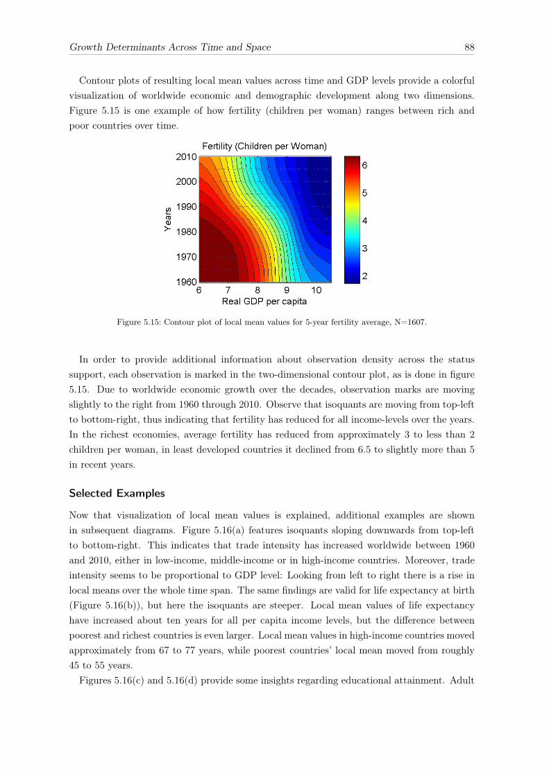
Growth Determinants Across Time and Space 88
Contour plots of resulting local mean values across time and GDP levels provide a colorfulvisualization of worldwide economic and demographic development along two dimensions.Figure 5.15 is one example of how fertility (children per woman) ranges between rich andpoor countries over time.
Figure 5.15: Contour plot of local mean values for 5-year fertility average, N=1607.
In order to provide additional information about observation density across the statussupport, each observation is marked in the two-dimensional contour plot, as is done in figure5.15. Due to worldwide economic growth over the decades, observation marks are movingslightly to the right from 1960 through 2010. Observe that isoquants are moving from top-leftto bottom-right, thus indicating that fertility has reduced for all income-levels over the years.In the richest economies, average fertility has reduced from approximately 3 to less than 2children per woman, in least developed countries it declined from 6.5 to slightly more than 5in recent years.
Selected Examples
Now that visualization of local mean values is explained, additional examples are shownin subsequent diagrams. Figure 5.16(a) features isoquants sloping downwards from top-leftto bottom-right. This indicates that trade intensity has increased worldwide between 1960and 2010, either in low-income, middle-income or in high-income countries. Moreover, tradeintensity seems to be proportional to GDP level: Looking from left to right there is a rise inlocal means over the whole time span. The same findings are valid for life expectancy at birth(Figure 5.16(b)), but here the isoquants are steeper. Local mean values of life expectancyhave increased about ten years for all per capita income levels, but the difference betweenpoorest and richest countries is even larger. Local mean values in high-income countries movedapproximately from 67 to 77 years, while poorest countries’ local mean moved from roughly45 to 55 years.Figures 5.16(c) and 5.16(d) provide some insights regarding educational attainment. Adult

Growth Determinants Across Time and Space 89
(a) (b)
(c) (d)
Figure 5.16: Contour plot of local mean values for (a) Trade share, N=1463, (b) Life expectancy at birth,N=1608, (c) Literacy rate of population (ages 15-49), N=675, (d) tertiary school enrollment ratio, N=1216.
literacy has been rising in all countries, but more so in poor and middle-income countries. Bylooking at literacy rates as a single indicator, it appears that the gap between high-incomecountries and the rest of the world has been narrowed over the years. Looking at tertiaryschool enrollment in Figure 5.16(d) as another indicator, downward sloping isoquants indicatea rise over all income-levels again. However, in this case the increase has been much larger forhigh-income countries. Therefore, this alternative indicator of educational attainment impliesthat the gap between rich and poor countries regarding higher education has widened.Figure 5.17(a) shows that the stock of migrants is much higher and growing in high-income
countries. This result is not surprising, since high-income countries appear more attractivethan low- and middle-income countries when people choose to migrate. The migration stockpercentage of the population in poor and middle-income countries has even been reduced overthe years. Finally, Figure 5.17(b) depicts local mean values of HIV prevalence between 1990and 2010. A maximum of infections has been recorded around the year 2000 in low-incomecountries. Since then, HIV casualties outweighed new infections such that the HIV prevalencein the population was reduced for the group of very poor countries. On the other hand,

Growth Determinants Across Time and Space 90
(a) (b)
Figure 5.17: Contour plot of local mean values for (a) Migration stock (% of total population), N=1668, (b)HIV prevalence (% of population ages 15-49), N=2709.
ascending isoquants for middle-income and richer countries suggest that overall prevalence ofHIV has sharply increased over time, even if average percentage levels for all income-levelsremain below 4 per cent, in high-income countries even below 1 per cent. Note that these areonly average levels of whole countries without considering population.The presented local mean value procedure offers a new way to visualize panel data. It
allows to investigate worldwide developments in demographic, macroeconomic and financialmeasures in a two-dimensional diagram.
5.6 Conclusion
This article applies functional coefficient analysis in the field of cross-country growth regres-sions. A panel data set of 145 countries between 1960 and 2010 was used, while focusing onmedium-run growth dynamics. Functional coefficients were determined in a one-dimensionalFCM with initial GDP as a status variable; and also in a two-dimensional FCM using the timedimension as a second status variable. Valuable insights can be generated from visualizationsof functional coefficients of both models.Instead of applying FCM to large multivariate models, whose results could hardly be consid-
ered robust, it was applied for the detailed investigation of bivariate relationships of economicgrowth. So the relationship of per capita growth rates with one variable at a time was investi-gated, namely investment, gross savings, foreign direct investment, government consumption,trade intensity, old age dependency ratio and tertiary educational attainment. For compar-ison, prefiltering of growth rates allowed to take established control variables of the Solowmodel into consideration. Estimated functional coefficients were qualitatively very similar tothe bivariate case. In the light of given results, showing that locally estimated coefficients ofgrowth determinants indeed vary strongly over time and also between poor and rich countries,it appears highly questionable to simply assume parameters to be constant as it is done in a

Growth Determinants Across Time and Space 91
conventional growth regression.Moreover, modeling economic relationships with functional coefficients allows a closer inves-
tigation of heterogeneity. It is possible to determine whether results of a constant coefficientmodel are primarily driven by a certain number of observations. The overall influence of acertain measure on a dependent variable may be strongly influenced by observations from acertain time period only, or by a subgroup of countries, while generalization of the finding forthe whole data set may be invalid. Hence, FCM may as well provide a sensitivity analysisand robustness check for OLS regression models in general.As a spin-off, the weighting scheme from FCM analysis can be used to compute a weighted
mean value for certain variables of interest. By computing and plotting these local meanvalues across the support of two status variables, a diagram is generated that visualizes paneldata. It is a colorful descriptive diagram, applicable for example in the field of developmenteconomics.

Growth Determinants Across Time and Space 92
5.7 References
[1] Aghion, P., Howitt, P. (2006), Appropriate Growth Policy: A Unifying Framework, in:Journal of the European Economic Association, 4 (2/3), 269–314.
[2] Baltagi, B. (2005), Econometric Analysis of Panel Data, 3rd ed., Chichester.
[3] Cai, Z., Fan, J. und Yao, Q. (2000), Functional Coefficient Regression Models for Non-linear Time Series, in: Journal of the American Statistical Association 95, 941–956.
[4] Durlauf, S.N. and Johnson, P.A. (1995), Multiple regimes and cross-country growth be-haviour. Journal of Applied Econometrics 10, 365–384.
[5] Durlauf, S.N., Kourtellos, A., Minkin, A. (2001), The local Solow growth model, in: TheEuropean Economic review 45, 928–940.
[6] Durlauf, S.N., Johnson, P.A., Temple, J. (2005), Growth econometrics, in: Aghion, P.,Durlauf, S.N. (2005), Handbook of economic growth, Amsterdam, 555–677.
[7] Jennen-Steinmetz, C. and Gasser, T. (1988). A unifying approach to nonparametricregression estimation. Journal of the American Statistical Association, 83, 1084–1089.
[8] Greene, W.H. (2003), Econometric Analysis, 5th ed., London.
[9] Härdle, W., Müller, M., Sperlich, S., Werwatz, A. (2004), Nonparametric and semipara-metric models, Berlin.
[10] Henderson, D. J., Papageorgiou, C. and Parmeter, C. F. (2012), Growth Empirics withoutParameters. The Economic Journal 122, 125–154.
[11] Herwartz, H. und Xu, F. (2007), A New Look at the Feldstein-Horioka Puzzle, UniversityKiel, Economics working paper 2007–14.
[12] Heston, A., Summers, R. and Aten, B. (2012), Penn World Table Version 7.1, Centerfor International Comparisons of Production, Income and Prices at the University ofPennsylvania, July 2012.
[13] Hodrick, R.J., Prescott, E.C. (1997), Postwar U.S. Business Cycles: An Empirical Inves-tigation, in: Journal of Money, Credit and Banking 29, 1–16.
[14] Ketteni, E., Mammuneas, T.P. and Stengos, T. (2007), Nonlinearities in economicgrowth: A semiparametric approach applied to information technology data, Journalof Macroeconomics 29 (3), 555–568.
[15] Kourtellos, A. (2002), Modeling Parameter Heterogeneity in Cross Country Growth Re-gression Models, University of Cyprus Discussion Paper 2002–12.

Growth Determinants Across Time and Space 93
[16] Levine, R., Renelt, D. (1992), A Sensitivity Analysis of Cross-Country Growth Regres-sions, American Economic Review 82(4), 942–963.
[17] Liu, Z. and Stengos, T. (1999), Non-linearities in cross-country growth regressions: asemiparametric approach. Journal of Applied Econometrics 14, 527–538.
[18] Lucas, R. (1988), On the Mechanics of Economic Development, Journal of MonetaryEconomics, 22, 3–42.
[19] Mamuneas, T.P., Savides, A. and Stengos, T. (2006). Economic development and the re-turn to human capital: a smooth coefficient semiparametric approach, Journal of AppliedEconometrics 21 (1), 111–132.
[20] Mankiw, N. G., Romer, D., and Weil, D. N. (1992). A Contribution to the empirics ofeconomic growth, Quarterly Journal of Economics 107(2): 407–437.
[21] McCartney, M. (2006), Can a Heterodox Economist Use Cross-Country Growth Regres-sions?, in: real-world economics review 37, 45–54.
[22] Nadaraya, E. (1964), On Estimating Regression, in: Theory of Probability and its Appli-cations 10, 186–190.
[23] Romer, P.M. (1986), Increasing Returns and Long-Run Growth, Journal of PoliticalEconomy 94, 1002–1037.
[24] Romer, P.M. (1990), Endogenous Technological Change, Journal of Political Economy99, 71–102.
[25] Sala-i-Martin, X., Artadi, E. (2004), The Global Competitiveness Index, in: Porter, M.et al. (Hrsg.), The Global Competitiveness Report, 2004-2005, Oxford University Press.
[26] Snowdon, B. (2006), The Enduring Elixier of Economic Growth. Xavier Sala-i-Martin onthe Wealth and Poverty of Nations, in: World Economics 7(1), 73–130.
[27] Solow, R.M. (1956), A contribution to the Theory of Economic Growth, Quarterly Jour-nal of Economics 70, 5–94.
[28] Vaona, A., Schiavo, S. (2007). Nonparametric and semiparametric evidence on the long-run effects of inflation on growth, Economic Letters 94(3), 452–458.
[29] Watson, G. (1964), Smooth Regression Analysis, in: Sankhya: The Indian Journal ofStatistics A 26, 359–372.
[30] World Bank (2012), World Development Indicators 2012, Washington, DC. Link:http://data.worldbank.org/data-catalog/world-development-indicators.

Growth Determinants Across Time and Space 94
5.A Appendix: List of Symbols
Symbol Descriptionβ̃ Parameter vectorβ̂(. . .) Locally estimated Parameter vectorβ0 Constantβ̃1 Vector of constant coefficient(s) (Prefiltering)β̃2(. . .) Vector of functional coefficient(s) (Prefiltering)βk k’th parameter in β̃βs Slope parameter for savingsei,t Residualh bandwidthh(. . .) local bandwidthi Country numberk Explanatory variable number in x̃i,tK Number of explanatory variablesKu Kernel function (Gaussian) for ui,tKw Kernel function (Gaussian) for wi,tN Number of countriesNeff Effective number of (weighted) observationsρ(. . .) Local correlationRSS Residual sum of squares (weighted)si,t Savings rate (explanatory variable)σ2x(. . .) Local variance of xi,tσ2y(. . .) Local variance of yi,tσxy(. . .) Local covariance between xi,t and yi,tt YearT Number of yearsui,t Status variableu Focus of local estimation in parameter space of ui,twi,t Additional status variable (time)w Focus of local estimation in parameter space of wi,txi,t Some variablex̃i,t Vector of explanatory variablesxi,t,k Explanatory variable in vector x̃i,tx( . . .) Local mean value of xi,t,k in one dimensionxlocal.. (. . .) Local mean value of xi,,kt in two dimensionsx̃1i,t Vector of explanatory variables with constant coefficientsx̃2i,t Vector of explanatory variables with functional coefficientsyi,t Dependent variable (growth rate)

CHAPTER 6
Charakteristika und Diffusion deutscher PRO-Patente
Ulrich StolzenburgInstitut für Vwl, Universität Kiel
&Joachim Tischler
Institut für Bwl, Universität Kiel
Abstract: Dieser Artikel charakterisiert die patentierten Forschungsergebnisse deutscher öffentlich fi-nanzierter Forschungseinrichtungen (PROs) und zeigt relevante Kennzahlen, Muster und Forschungsschwer-punkte auf. Hierbei wird nach Untergruppen institutionell verbundener Forschungseinrichtungen (Forschungs-familien) differenziert. Schließlich wird die Weiterverfolgung und Verwertung dieser Patente in unterschiedlicheLänder skizziert, wiederum unter Berücksichtigung von Technologiefeldern und Forschungsfamilien.
Erschienen in: Walter, Achim (Hrsg., 2014): "Wirtschaftliche Bedeutung des patentierten grundlagenorien-tierten Wissens in Deutschland", Hannover: Technische Informationsbibliothek Hannover. Schlussberichtdes BMBF-Forschungsvorhabens, Projektlaufzeit: 01.07.2010 bis 31.07.2013, kostenneutral verlängert bis30.09.2013. Auftragnehmer: Christian-Albrechts-Universität zu Kiel, Wirtschafts- und SozialwissenschaftlicheFakultät, Lehrstuhl für Gründungs- und Innovationsmanagement. Kapitel 5 (S.74–104).

Eidesstattliche Erklärung
Ich erkläre hiermit an Eides Statt, dass ich meine Doktorarbeit “Essays on Economic Growthand Business Cycle Dynamics” selbständig und ohne fremde Hilfe angefertigt habe und dass ichalle von anderen Autoren wörtlich übernommenen Stellen, wie auch die sich an die Gedankenanderer Autoren eng anlehnenden Ausführungen meiner Arbeit, besonders gekennzeichnetund die Quellen nach den mir angegebenen Richtlinien zitiert habe.
Ich versichere an Eides Statt, dass ich mich an keiner anderen Fakultät einer Doktorprüfungunterzogen habe.
Kiel,
(Ulrich Stolzenburg)

Lebenslauf
Persönliche DatenName Ulrich StolzenburgGeburtsdatum 05.06.1979Geburtsort Bremen
Jahr Tätigkeitbis 08/1998 Gymnasiale Oberstufe, Schulabschluss: Abitur (Durchschnittsnote 1,7),
Schulzentrum im Holter Feld, Bremen.09/1998 - 02/2001 Ausbildung zum "Mathematisch-Technischen Assistent / Informatik
(IHK)" bei "STN Atlas Elektronik GmbH", Bremen.03/2001 - 08/2001 Beschäftigung als Software-Assistent im Anschluss an die Berufsausbildung
bei "STN Atlas Elektronik GmbH", Bremen.10/2001 - 07/2007 Studium der Volkswirtschaftslehre an der Christian-Albrechts-Universität
Kiel, Schwerpunkt: Quantitative Wirtschaftsforschung, Wahlpflichtfach:Internationale Wirtschaftsbeziehungen. Abschluss: Diplom ("Sehr Gut",Durchschnittsnote 1,4)
01/2008 - 12/2008 Nebenberufliche Tätigkeit bei der "HSH Financial Markets Advisory", Kiel.11/2008 - 12/2013 Nebenberufliche Tätigkeit bei "Analytix GmbH - Institut für statistische
Datenanalyse und quantitative Marktforschung", Kiel.01/2011 - 12/2013 Wissenschaftlicher Mitarbeiter am Institut für Betriebswirtschaftslehre,
Lehrstuhl für Gründungs- und Innovationsmanagement (Prof. AchimWalter), Universität Kiel, im Rahmen des BMBF-Forschungsprojektes"Wirtschaftliche Bedeutung des patentierten Grundlagenwissens inDeutschland".
10/2007 - 02/2015 Teilnehmer im Doktorandenprogramm "Quantitative Economics" derWirtschafts- und Sozialwissenschaftlichen Fakultät der Christian-Albrechts-Universität Kiel. Abgabe der kumulativen Dissertation mitdem Titel "Essays on Economic Growth and Business Cycle Dynamics"am 17.12.2014, mündliche Doktorprüfung am 18.2.2015. Gesamtnote:"Summa Cum Laude".