Estimation of Joint Income-Wealth Poverty:A Sensitivity Analysis

Sarah Kuypers1 • Ive Marx1,2

Accepted: 6 December 2016� Springer Science+Business Media Dordrecht 2016

Abstract Most poverty studies build on measures that take account of recurring incomes

from sources such as labour or social transfers. However, other financial resources such as

savings and assets also affect living standards, often in very significant ways. Previous

studies that have sought to incorporate assets into poverty measures agree that (1) poverty

estimates including wealth are considerably lower than the traditional income-based

measures; (2) poverty rates of the elderly are more affected than those of the non-elderly

and (3) poverty rates are especially affected by the household’s main residence. This paper

assesses the sensitivity of these conclusions to various plausible alternative assumptions,

such as the poverty line calculation, the types of assets included in the wealth concept and

choices with respect to the equivalence scale. Moreover, we check whether the impact of

alternative assumptions is consistent across age and institutional settings. To that effect we

compare Belgium and Germany, two countries with similar living standards and income

poverty rates, but very different levels and distributions of wealth. Using data from the

Eurosystem Household Finance and Consumption Survey we show that accounting for

wealth affects the incidence and age structure of poverty in a very substantial way.

However, we also illustrate that results strongly depend on all kinds of measurement

choices. We show that poverty rates may increase as well as decrease depending on how

The authors gratefully acknowledge financial support from the Belgian Science Policy Office (BELSPO)under contract BR/121/A5/CRESUS. We would like to thank Koen Decancq, Gerlinde Verbist and par-ticipants of the 2015 Spring Meeting of the ISA RC28, the 2015 LISER/DSEF Joint PhD Workshop, the2016 Improve Final conference and 34th IARIW General Conference 2016 for their helpful comments andsuggestions on earlier versions of this paper.

& Sarah Kuyperssarah.kuypers@uantwerpen.be

Ive Marxive.marx@uantwerpen.be

1 Herman Deleeck Centre for Social Policy, University of Antwerp, Sint-Jacobsstraat 2,2000 Antwerp, Belgium

2 IZA, Bonn, Germany

123

Soc Indic ResDOI 10.1007/s11205-016-1529-5

wealth is accounted for. Cross-country rankings may also change, overall or for specific

groups. Second, current measures are not representative for young households such that

any conclusion on the age ratio of poverty is highly sensitive to the assumptions made.

Keywords Income � Wealth � Poverty measurement � Sensitivity analysis

JEL Classification I32

1 Introduction

Researchers and policy makers in the rich world mostly worry about income poverty.

However, the wider financial resources on which people can draw are also important in

assessing financial precariousness. Households that can smooth out consumption by relying

on savings and assets, loans or the financial help of others are clearly better off than

households who do not have these opportunities. Yet, apart from the direct income flows

they may generate, traditional poverty measures often disregard the role of such assets

(Azpitarte 2011; Brandolini et al. 2010). In contrast, financial liabilities may make

households more economically vulnerable than their incomes suggest. Moreover, evidence

also shows that wealth and income have an independent impact on subjective well-being

(Headey and Wooden 2004) and on satisfaction of life (D’Ambrosio et al. 2009). Recent

high-level reports also argue in favour of a joint income-wealth perspective on living

standards (Stiglitz et al. 2009; OECD 2013b).

If one agrees on the fact that wealth should be included in poverty measurement, the

question arises: how should we do it? In the literature there are two approaches. A first

approach integrates the two financial resources into one single dimension by converting

wealth into yearly annuities (Brandolini et al. 2010; Short and Ruggles 2005; Van den

Bosch 1998; Weisbrod and Hansen 1968), while a second approach applies a two-di-

mensional framework by developing separate poverty lines for income and wealth (Kim

and Kim 2013; Azpitarte 2012; Headey 2008; Haveman and Wolff 2004). The general

findings of these approaches are (1) that poverty estimates including wealth are much

lower than the traditional income-based measures; (2) that poverty rates of the elderly are

much more affected than those of the non-elderly and (3) that the decline in poverty rates is

much higher when the value of the household’s main residence is included than when only

non-housing wealth is taken into account (Azpitarte 2012; Brandolini et al. 2010; Headey

2008; Caner and Wolff 2004; Van den Bosch 1998). However, we may want to be careful

about generalizing these findings of a limited number of studies. Indeed, ‘‘we need to better

understand the properties of these alternative indicators and assess their sensitivity to

different assumptions’’ (Brandolini et al. 2010, p. 281).

The purpose of this paper is exactly this. We investigate several issues related to the

measurement of joint income-wealth poverty. We discuss in detail the two approaches

adopted in the literature and empirically review the robustness of poverty outcomes to

various measurement assumptions, such as the use of different poverty lines, wealth

concepts, equivalence scales, etc. Moreover, we also highlight the sensitivity of the results

from the angle of age. This after all is the socio-demographic characteristic which is

thought to be the most sensitive to the way we include wealth information. We use income

and wealth data from the Eurosystem Household Finance and Consumption Survey

(HFCS) for Belgium and Germany. These countries are known for having very similar

S. Kuypers, I. Marx

123

living standards and income poverty rates, but appear to have very different levels and

distributions of wealth, and which are differently correlated with income. We show that the

two most important conclusions drawn in the literature largely depend on specific mea-

surement choices. First, studies generally find that poverty estimates including wealth are

much lower than the traditional income-based measures. We show that this strongly

depends on the way one calculates the poverty line. Poverty rates may increase as well as

decrease after wealth is accounted for, substantially altering cross-country rankings. Sec-

ond, as one would expect, the inclusion of wealth has a great effect on the observed poverty

incidence among young versus older households, yet any conclusion on the ratio between

elderly and non-elderly poverty is again highly sensitive to the assumptions that are made.

The paper proceeds as follows. The second part discusses the literature on joint income-

wealth poverty and its relationship to the traditional poverty literature. More specifically,

we highlight several reasons why it is important to include wealth in the measurement of

poverty and how in practice this is implemented by the two approaches. The data are

briefly described in the third part and the fourth part presents the baseline results for

Belgium and Germany. In the following part we address the choices that researchers need

to make in the operationalisation of the joint income-wealth poverty index and we perform

sensitivity analyses for several of these measurement issues. In particular, we consider the

robustness of our outcomes to variations in the following aspects: the poverty line, wealth

concept, equivalence scale and the interest rate. The last part concludes.

2 Measuring Poverty

2.1 Why Include Wealth in Poverty Measurement?

‘‘Although poverty reduction is a universal goal among both nations and international

organizations, there is no commonly accepted way of identifying who is poor.’’ (Haveman

and Wolff 2004, p. 146). However, the concept of poverty usually refers to a situation of

economic hardship, when the financial resources over which people have command are

insufficient to guarantee a minimally acceptable standard of living. A definition of poverty

requires an identification of ‘financial resources’ and a method to determine the minimally

acceptable living standard. In a developed context, the first is typically expressed in terms

of yearly or monthly disposable income, while the latter is more contested. In the EU the

most important poverty indicator is the At-risk-of-poverty (AROP) measure, which sets the

poverty threshold at 60% of national median equivalised disposable household income.

This income concept covers income from labour, pensions and social transfers as well as

financial income such as interests, dividends, etc.

Hence, apart from the direct income flow they generate, the role of assets is absent

(Azpitarte 2011; Brandolini et al. 2010). Since there are also assets that generate little or no

income flow this approach is not satisfying. Moreover, evidence shows that estimates of

capital income and self-employment income (which often also includes some type of

capital income) are typically underestimated in household surveys (Mattonetti 2013;

Davies et al. 2011; Wagner and Grabka 1999 as cited by Milanovic 2006). The most

evident example of an asset that is currently not represented in poverty measures is

housing. A solution to this problem has been suggested by adding to income the concept of

‘imputed rent’, which is the estimated value of housing services provided by owner-

occupied dwellings less the value of costs incurred to maintain the property (Canberra

Estimation of Joint Income-Wealth Poverty: A Sensitivity…

123

Group 2011). However, this addition is not sufficient because savings and assets contribute

to living standards above and beyond the direct income flows they generate. They assure

economic and financial security because they can be used to face unexpected financial

setbacks. Moreover, assets provide their owners with a form of economic power by

enabling them to make purchases to move up or maintain class status (Cowell and Van

Kerm 2015; Nam et al. 2008). In other words, assets contribute to living standards not only

by generating income flows but also because they can be converted directly into cash or

can be used as collateral (Azpitarte 2012). In contrast, the presence of large financial

liabilities might also be incorporated in poverty measurement because it may make

households much more vulnerable than their mere incomes suggest. Furthermore, because

income is by nature rather volatile, evidence shows a large turnover in income poverty

(Azpitarte 2012), while assets and liabilities are much more stable. For these and other

reasons several authors have argued in favour of including information on wealth in

poverty measurement because it better reflects all the financial resources available to

households (e.g. Azpitarte 2012; Brandolini et al. 2010; OECD 2013a, b; Stiglitz et al.

2009).

Many authors would take these critiques as arguments for using consumption infor-

mation. Indeed, as it reflects the difference between income and the change in net worth it

might be sufficient to look at this single dimension instead of trying to integrate two

resources. The large drawback of this approach, however, is that it only looks at actual

consumption patterns. Particularly in the case of wealth, households may want to decide

not to use all available resources for consumption. Imagine two households with the same

low income and median wealth; it is not because the first household decides to use their

wealth to support consumption and the second household does not that the latter is nec-

essarily worse off. In the words of Sen (1985, 1997), we should look at all available

resources to be able to identify the capability set of households. Combining information on

income and wealth allows to determine all consumption possibilities (Stiglitz et al. 2009,

p. 115).

2.2 How Include Wealth in Poverty Measurement?

In a developed context there exist two main approaches to take account of the contribution

of assets to households’ living standards. The first one summarizes the wealth and income

dimensions into a unidimensional poverty index. Since wealth is a stock and income a flow

the annuity method proposed by Weisbrod and Hansen (1968) is often used in order to

make assets ‘‘commensurable’’ (p. 1315). The method is adopted by among others Bran-

dolini et al. (2010), Short and Ruggles (2005), Zagorsky (2005) and Van den Bosch (1998).

The second approach follows a two-dimensional approach by developing separate poverty

lines for income and wealth. The most notable contributions in this stream are Azpitarte

(2011, 2012), Headey (2008) and Haveman and Wolff (2004). We discuss both approaches

below in more detail, with a graphical illustration provided in Fig. 1.

First, the unidimensional approach defines poverty by the sum of income and wealth. In

general it is considered too extreme to expect households to use all their wealth to keep

living standards at an adequate level. Therefore, the method of Weisbrod and Hansen

(1968) to annuitize wealth is used. Wealth is converted into a flow of resources, so as to

end up with an augmented income concept (Azpitarte 2011; Brandolini et al. 2010).

‘‘Income and wealth are perfectly fungible, and one unit of wealth can be straightforwardly

substituted for one unit of income’’ (Brandolini et al. 2010, p. 269). This seems intuitive

because most assets are the result of an accumulation of income and can be converted back

S. Kuypers, I. Marx

123

into income (Kim and Kim 2013).1 The annuitization is specified using the following

formula:

AYt ¼ Yt þq

1� 1þ qð Þ�n

� �NWt�1

n ¼ T for unmarried;

T1 þ T � T1ð Þb for married

ð1Þ

(Brandolini et al. 2010, p. 270).

Where AYt refers to annuitized income, Yt equals income received in year t, NWt-1 is net

worth held at the beginning of the period and q and n are the interest rate and length of the

annuity respectively. The latter is expressed in terms of life expectancies, where T1 refers

to time to death of the person who dies first, T time to death of the survivor and b is the

reduction in the equivalence scale coefficient which results from the death of the first

person (for a detailed derivation of this formula see Brandolini et al. 2010, pp. 269–271,

273).2 Income (Yt) should be interpreted as net of the yield from net worth because this

yield would be lost if net worth is depleted (Weisbrod and Hansen 1968, p. 1317). In other

words, Yt only covers income received from labour, pensions and social transfers and not

financial income. A nuance that should be added to this, however, is that annuities exist as

distinct financial products. As this flow originates from assets that are no longer in pos-

session of the household it should also be added to the income variable.

The main critique on this first approach is that it aggregates all available information so

that it does not allow studying differences in income and wealth positions (Azpitarte 2012).

1 It should be clear that not all asset types can be easily sold or bought on the market. In the case of non-liquid assets like real estate it is certain that an immediate sale would mean incurring substantial costs.2 The specification of n in function of expected lifetimes of both partners is proposed by Rendall and Speare(1993). Although Brandolini et al. (2010) discuss this broader specification, they do not implement it. Asmost authors they use the longest of the two expected lifetimes. We prefer to use the Rendall and Spearespecification because it represents the improved economic situation of the surviving household as the samelevel of wealth is then available to fulfill the needs of fewer household members. Ideally, one should takeinto account the wealth loss due to inheritance taxes.

Only asset poor

Income poverty threshold

Asset poverty threshold

Poverty threshold when all wealth is taken into account

Annui�zed income-net

worth povertythreshold

Income poverty threshold

(a) (b)

Only incomepoor

Income & asset

poor

Y Y

NW NW

Fig. 1 Illustration of poverty lines. a Unidimensional poverty index, b two-dimensional poverty index.Source: Brandolini et al. (2010, pp. 270, 272)

Estimation of Joint Income-Wealth Poverty: A Sensitivity…

123

Second, it is argued that the single income-net worth approach obliges researchers to

impose several assumptions, mainly regarding the values of the length and interest rate of

the annuity. ‘‘We might be reluctant to impose so much structure on the measurement,

especially when we take into account the profound implications that such a measure has for

the age structure of poverty.’’ (Brandolini et al. 2010, p. 271). Finally, Weisbrod and

Hansen (1968) stress that they developed an approach that is operationally feasible, but

may not reflect how households handle their assets in practice. Indeed, they do not imply

‘‘[…] either that people generally do purchase annuities with any or all of their net worth,

that they necessarily should do so, or that they can do so’’ (pp. 1316–1317).

The second approach specifies poverty thresholds for each dimension separately. In this

regard income poverty retains its traditional interpretation, while asset poverty3 is seen as

the situation where asset holdings are insufficient to maintain the household at a minimally

acceptable living standard when income from labour or social transfers is not available

(Brandolini et al. 2010; Haveman and Wolff 2004). In other words, wealth adds a sort of

sustainability aspect to the definition of poverty (Tormalehto et al. 2013). Haveman and

Wolff (2004) and Caner and Wolff (2004) use the following operational definition: ‘‘a

household or a person is considered to be asset poor if their access to wealth-type resources

is insufficient to enable them to meet their basic needs for some limited period of time’’.

More specifically, they set the asset poverty threshold as a fraction (f) of the official

income poverty line (Zt), which can be formalised as follows:

Asset poverty : NWt�1\fZt

Income poverty : Yt\Z � rtNWt�1

ð2Þ

(Brandolini et al. 2010, p. 271).

This approach enables one to identify three types of poverty groups, and hence provides

an answer to the first critique. First, there are households which are poor in both dimen-

sions. Second, there is a group of households that fall under the income poverty line, but

can rely on substantial amounts of assets. Finally, households may have an income above

the income poverty threshold, but are asset poor because they own little or no assets to fall

back on (Azpitarte 2012). Headey (2008) also applies this approach to the measurement of

poverty in Australia but takes into account a third dimension, namely consumption. The

reason is mainly that it reflects borrowing opportunities. However, for reasons explained in

Sect. 2.1 and because borrowing opportunities are correlated with income and wealth (e.g.

Azpitarte 2012; Sullivan 2008) (i.e. they tend to be unavailable to those with both low

income and low wealth), it is sufficient to jointly look at income and wealth poverty.

3 Data and Methods

We use data from the first wave of the HFCS version 1.1. The HFCS is a rich dataset

covering detailed wealth, gross income and consumption information of more than 62,000

households in 15 Euro area member states [Eurosystem Household Finance and Con-

sumption Network (HFCN) 2013a, b]. In Belgium 2327 households were surveyed in 2010,

while the German HFCS covers information on 3565 households and surveys took place in

3 Authors tend to refer to wealth poverty when implementing the unidimensional approach, while the termasset poverty is mostly used for the two-dimensional approach. As both approaches use net worth in theircalculations, this reflects only a difference in terminology.

S. Kuypers, I. Marx

123

2010 and 2011. For both countries incomes refer to 2009, while the value of assets and

liabilities refers to the time of the interview. Noteworthy features of the HFCS are over-

sampling of the wealthy,4 multiply imputed data and replicate weights.

3.1 Belgium and Germany as Case Studies

This paper builds on Belgium and Germany as case studies. These neighbouring countries

belong to the most advanced economies in Europe and their social security systems are

both largely founded on Bismarckian principles. Both countries rely on pay-as-you go

pension systems. What makes the two countries particularly interesting is that while

median living standards and overall poverty rates are nearly identical, their levels and

distributions of private household wealth differ completely.

As can be seen in Table 1, median equivalised incomes are almost the same and the

traditional AROP rate is at a similar level in both countries. However, Table 1 also shows

that median wealth accumulations are much higher in Belgium than in Germany. This

difference is mainly the consequence of a significant discrepancy in the home-ownership

rate. About 70% of Belgian households own their house, but although many countries have

similar home-ownership rates today, Belgium has been a ‘nation of homeowners’ for a

long time already (De Decker 2011). This is the consequence of a century of an ‘‘asset-

based approach to welfare’’ (De Decker and Dewilde 2010) in which homeownership was

highly encouraged through various policy mechanisms. In contrast, Germany has at 44%

the lowest home-ownership rate in the Euro Area, which ‘‘[…] can be explained by

historical (WW2), taxation and institutional reasons’’ (HFCN 2013b, p. 29). Moreover, the

correlation between the income and wealth distributions is weaker in Belgium than in

Germany (Arrondel et al. 2014; Skopek et al. 2012). In particular, Belgium has a relatively

large share of households with low incomes but substantial wealth holdings, which are

mainly represented among the elderly population (Arrondel et al. 2014; Van den Bosch

1998). As a result of the combination of higher wealth levels and a weaker correlation with

income, we expect that the inclusion of wealth in poverty measurement will have a larger

impact in Belgium than in Germany.

3.2 Methods

With regard to wealth we use the HFCS ‘net worth’ concept (see first column of Table 3

for an overview of its components), which does not include asset types such as human and

social capital or the valuation of pension and social security wealth. The HFCS covers only

gross incomes, which are not suitable for poverty analysis. However, for several countries

these have been converted into disposable incomes5 using the tax-benefit microsimulation

model EUROMOD (see Kuypers et al. 2015).6 For the traditional income poverty we use

the EU At-risk-of-poverty line (AROP), which is defined as 60% of national median

equivalised disposable income. The income variable that is implemented in the two-di-

mensional approach refers to disposable income, while the income variable in the unidi-

mensional approach covers only income from employment, self-employment, public and

4 In Belgium this oversampling was based on the NUTS 1 region and the average income by neighbourhoodof residence.5 Property taxes could not be taken into account because the HFCS does not include cadastral values.6 A Eurostat study (2013) proposes another method to jointly assess poverty in disposable income and netwealth. By statistically matching the EU-SILC and HFCS data they largely find the same results.

Estimation of Joint Income-Wealth Poverty: A Sensitivity…

123

private pensions and social and private transfers. As annuity products are uncommon in

Europe, these types of assets are not surveyed in the HFCS.

Formulas (1) and (2) require income in year t and net worth at the beginning of that

year. Since the HFCS combines information on income during the last 12 months/calendar

year and net worth at time of survey, there could be some resources that are represented in

both income and net worth. This type of ‘double counting’ exists with regard to income

that is received during year t which is not consumed but instead saved or invested.7 The

problem is that it is not clear which part of wealth at the end of the year originated from

income received throughout the year. We propose to exclude from wealth an amount equal

to the income from financial investments, such as dividends, interests and rental income

from property. This appears to be a good proxy because evidence shows that people are

more likely to save from irregular income sources such as financial income than from

regular wages and salaries (Shefrin and Thaler 1992; Thaler 1990 as cited by Beverly et al.

2008). Indeed, since financial income is rather insecure it is often not accounted for in

household budgeting, which makes it easier to set aside. Moreover, it will be easier to save

or invest financial income because it already originates from the financial sphere and the

costs of reinvestment are smaller.

In order to calculate the annuity in the unidimensional approach we use life

expectancies by age and gender which are provided by the Directorate-General Statistics,

Department Economics of the Belgian Federal Government (2014) and the Statistisches

Bundesamt (2012). Since age is top coded at 85 years in the HFCS we restrict our analysis

to households where both partners are maximum 84 years old.8

4 Baseline Results

We start our empirical discussion by looking at poverty headcounts for Belgium and

Germany when implementing the standard assumptions of the literature, our so-called

‘baseline indicators’. The unidimensional approach to joint income-wealth poverty is in

most studies operationalised by setting the interest rate (q) equal to 2% and the poverty line

is set equal to the official income poverty line (e.g. Brandolini et al. 2010; Van den Bosch

1998; Weisbrod and Hansen 1968). The parameters of the two-dimensional approach are in

existing studies determined as follows: the income poverty line retains its traditional

7 Also saved income from the ongoing year can be represented in the net worth measure. As we have noinformation on current incomes we cannot correct for this.8 We cannot assign life expectancies if we do not have information on the exact age. As a consequence forboth countries about 80 sample households were not included in the analysis.

Table 1 Comparison of social indicators Belgium and Germany. Source: Eurostat, HFCN (2013a)

Belgium Germany

Median equivalised disposable incomea €19,313 €18,586

At-risk-of-poverty ratea 14.6% 15.5%

Median net wealth €206,000 €51,000

Home-ownership rate 69.6% 44.2%

a We use data from 2009, in line with the HFCS income reference period

S. Kuypers, I. Marx

123

interpretation and the asset poverty line is set at � of the income poverty line (e.g.

Azpitarte 2012; Haveman and Wolff 2004). Based on these choices the general findings of

the literature are first that the estimates are much lower than for the traditional income-

based measures. This is not surprising as they tend to keep the traditional poverty line

constant while including considerably more financial resources to the measure that is

evaluated against this poverty line. Second, as a consequence of the life-cycle model of

wealth accumulation poverty rates of the elderly are much more affected than those of the

non-elderly. Finally, since housing wealth represents the largest share of a household’s

asset portfolio the decline in poverty rates is much higher when the value of the house-

hold’s main residence is included than when non-housing wealth is only taken into account

(e.g. Azpitarte 2012; Brandolini et al. 2010; Caner and Wolff 2004).

The results of the baseline indicators for our two countries are shown in Table 2. In line

with previous studies we find lower poverty rates when wealth is incorporated in the

measurement of poverty compared to the traditional income poverty headcount, but the

impact differs largely between countries. The unidimensional approach suggests a decrease

of the number of poor households with 5.7% points for Belgium and with 2.2% points for

Germany. Outcomes for the two-dimensional approach indicate that about 6.2% of Belgian

households are both income and asset poor, while almost 11% have an income below the

poverty threshold but own substantial amounts of wealth, which is about two-thirds of all

income-poor households. Interestingly, 5.6% of households are not considered poor

according to the traditional income poverty line, but they have little or no assets to fall

back on, which makes them very vulnerable to an income loss. Among German households

the three groups represent about the same share. Less than half of all income poor

households are found to have sufficient wealth holdings. These outcomes confirm our

expectations; because wealth levels are lower in Germany and more correlated with

income, the inclusion of wealth information has a much weaker impact in Germany than in

Belgium.

Table 2 also provides results separately for the elderly and non-elderly.9 It is clear that

the inclusion of wealth has a much larger impact on the number of poor elderly than non-

elderly, which also corresponds to evidence from other studies. Again, the effect is larger

among the Belgian elderly than among the German elderly.

5 Sensitivity Analysis

The next step is to assess the robustness of these results to various measurement issues. In

the first section we consider how to determine the poverty line when taking a joint income-

wealth perspective on poverty. Several other issues related to the measurement of joint

income-wealth poverty are discussed in the second section, such as the wealth concept that

is adopted, the impact of equivalence scales and differing interest rates. The last section

focusses on the age structure of poverty.

5.1 Poverty Line

The most important choice when operationalising any poverty measure is where to draw

the poverty line. In case of the unidimensional approach it reflects whether or not to adapt

9 Elderly is defined as at least one of the adults being 65 years or older, the legal retirement age in Belgiumand Germany.

Estimation of Joint Income-Wealth Poverty: A Sensitivity…

123

the single poverty line to the inclusion of wealth information. Prior studies often only

change the sources which are taken into account to assess living standards and evaluates it

against the classic income poverty line (this is also what we have done in the baseline

indicator in Table 2). This is compatible with the view that the current income poverty line

reflects the true resources needed by households to sustain an acceptable living standard.

As shown above, this choice results in lower poverty estimates which are believed to be

closer to the true level of poverty (see e.g. Brandolini et al. 2010; Van den Bosch 1998;

Weisbrod and Hansen 1968).

A competing view argues that the income poverty line was initially set to represent a

‘standard’ level of resources, whereby different poverty lines are determined for example

for homeowners and tenants. If wealth is accounted for as a financial resource, then the

poverty line should be adjusted upwards in order to reflect the fact that it implies a higher

level of consumption possibilities (Lerman and Mikesell 1988, p. 360). The poverty line

would then be set as a percentage of ‘median equivalised income ? annuitized net worth’.

As Brandolini et al. (2010, p. 275) argue this is ‘‘more consistent with a fully relative

approach’’. Figure 2 shows the poverty rate for different percentages of median equivalised

income-net worth. In contrast to the baseline results in Table 1, the poverty headcount is

Table 2 Baseline poverty rates. Source: own calculations based on HFCS

Poverty measure All Elderly (65–84) Non-elderly (–64)

Belgium Germany Belgium Germany Belgium Germany

Income povertya 17.1 18.5 14.2 16.6 18.1 19.2

Unidimensional 11.4 16.3 3.5 11.9 14.1 18.0

Two-dimensional

Income and asset poor 6.2 9.7 1.4 5.7 7.9 11.3

Only income poor 10.9 8.7 12.8 10.9 10.2 7.9

Only asset poor 5.6 11.1 4.2 6.0 6.1 13.0

Unidimensional poverty is calculated using unadapted poverty line (i.e. traditional income poverty line) (seeSect. 5.1)a The results based on the HFCS are slightly higher than the official income poverty rates reported byEurostat (see Table 1). This is the consequence of the combination of a slightly higher median income in theHFCS than in other surveys and lower disposable incomes at the bottom of the distribution (Kuypers et al.2015). Moreover, in contrast to the general evidence on income poverty (OECD 2008; Eurostat), thetraditional income poverty measure based on the HFCS suggest a smaller incidence among elderly thanamong non-elderly

0

10

20

30

40

50

60

0 5 10 15 20 25 30 35 40 45 50 55 60 65 70 75 80 85 90 95 100

Pove

rty

rate

Poverty line (% of median annui�zed income-net worth)Belgium Germany

Fig. 2 Effect of a relativepoverty line on poverty rates.Source: own calculations basedon HFCS

S. Kuypers, I. Marx

123

considerable lower in Germany than in Belgium up until a poverty line at 45% of median

annuitized income-net worth, while poverty lines at higher percentages result in very

similar poverty rates in the two countries. For instance, if we would set it at 60% such as in

the AROP then the share of poor households would be equal to 21.3% in Belgium and

21.8% in Germany.

Hence, the conclusion of the literature that poverty rates decline when wealth is taken

into account largely depends on the assumption that the poverty line is not adapted to the

broader resources concept. The poverty headcount can both increase as decrease and this

may have a substantial impact on cross-country rankings. The remainder of the sensitivity

analyses will all use the 60% of median equivalised income-net worth (hence, the baseline

indicator is the one from Table 1 but with an adapted poverty line).

In the two-dimensional approach to income-wealth poverty a similar issue arises. In this

approach the asset poverty line is typically defined in function of the income poverty

threshold. It would also be possible to define the asset threshold in function of another

approximation of a minimally acceptable living standard, for example the household

budget standard. Moreover, one could just as well think of some absolute asset poverty

threshold, such as the asset poverty line of $200,000 implemented by Headey (2008).

Sherraden (1991) argues that in terms of political reality an absolute perspective on asset

poverty is more valid than a relative one. Finally, Bucks (2011) uses a subjective measure

of ‘assets/savings adequacy’ by evaluating the assets available to households to their

desired level of precautionary savings, i.e. the amount of savings households themselves

consider to be sufficient to cover unanticipated expenses.

When deciding to set the asset poverty line as a fraction of the income poverty

threshold, a second choice involves at which fraction it should be set. In other words, what

is the time period households are supposed to sustain themselves at the official poverty line

without income from work or other sources. In existing studies the asset poverty threshold

is generally set at one-fourth, which means that households need to have sufficient wealth

to keep them at the income poverty line for at least 3 months. The rationale provided for

this is that unemployment is regarded as the most important cause of economic hardship,

for which the expected duration in the United States, prior to the financial crisis, was

between 2 and 4 months (McKernan et al. 2012; Haveman and Wolff 2004; Caner and

Wolff 2004). However, expected unemployment duration is typically longer in Europe than

in the US (OECD 2014, p. 96) and also longer as a consequence of the crisis. Therefore, we

assess the sensitivity of the poverty rate for periods between 1 month and a year, which is

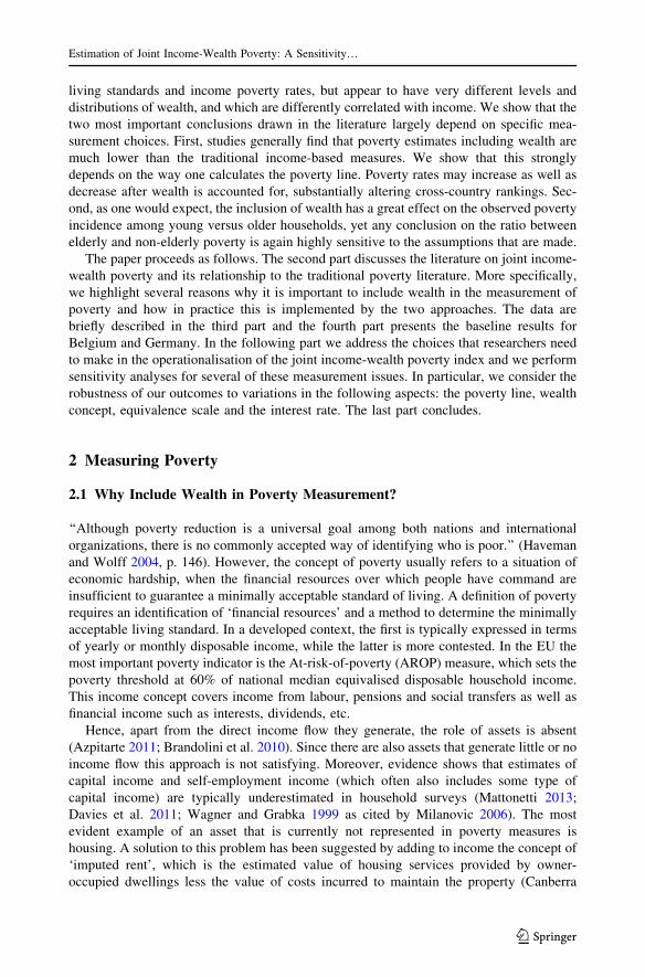
shown in Fig. 3.

As expected, the longer households are supposed to sustain themselves at the official

income poverty line the larger the share of the categories of income and asset poor and

only asset poor and the lower the share of those who are only income poor. For example, if

households need to be able to sustain themselves at the income poverty threshold for 6

instead of 3 months solely drawing on their wealth the number of income and asset poor

increases by about 1.5% points in both countries, which reflects a shift from the group who

is only income poor. At the same time the share of households which are only asset poor

increases with around 2 and 3.5% points in Belgium and Germany respectively. This

means that a non-negligible share of households have enough wealth accumulations to

sustain themselves for 3 months at the income poverty line, but not for 6 months. Fur-

thermore, the cross point where the share of only asset poor households becomes higher

than the share of the only income poor is already at an asset poverty line of 2 months in the

case of Germany, while it is found only at 8 months for Belgium. In other words, of those

Estimation of Joint Income-Wealth Poverty: A Sensitivity…

123

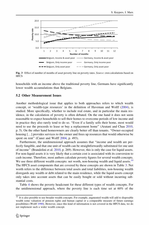
households with an income above the traditional poverty line, Germans have significantly

lower wealth accumulations than Belgians.

5.2 Other Measurement Issues

Another methodological issue that applies to both approaches refers to which wealth

concept, or ‘wealth-type resources’ in the definition of Haveman and Wolff (2004), is

studied. More specifically, whether to include real estate, and in particular the main res-

idence, in the calculation of poverty is often debated. On the one hand it does not seem

reasonable to expect households to sell their homes to overcome periods of low income and

in practice they also rarely tend to do so. ‘‘Even if a family sells their home, most would

need to use the proceeds to lease or buy a replacement home’’ (Aratani and Chau 2010,

p. 5). On the other hand homeowners are clearly better off than tenants. ‘‘Owner-occupied

housing […] provides services to the owner and frees up resources that would otherwise be

spent on rent’’ (Caner and Wolff 2004, p. 493).

Furthermore, the unidimensional approach assumes that ‘‘income and wealth are per-

fectly fungible, and that one unit of wealth can be straightforwardly substituted for one unit

of income’’ (Brandolini et al. 2010, p. 269). However, this is only the case for liquid assets.

For non-liquid assets it is very likely that a certain cost is associated with its conversion to

cash income. Therefore, most authors calculate poverty figures for several wealth concepts.

We use three different wealth concepts: net worth, non-housing wealth and liquid assets.10

The HFCS asset components that are covered by these concepts are shown in Table 3. Net

worth refers to the difference between total assets and total liabilities, non-housing wealth

disregards any wealth or debt related to the main residence, while the liquid assets concept

only takes into account assets that can be easily bought or sold without incurring sub-

stantial costs.

Table 4 shows the poverty headcount for these different types of wealth concepts. For

the unidimensional approach, where the poverty line is each time set at 60% of the

10 It is also possible to use broader wealth concepts. For example, augmented wealth will add to disposablewealth some valuation of pension rights and human capital or a comparable measure of future earningspossibilities (Wolff 1990). However, since this kind of information is not covered in the HFCS data, we donot implement such a wider wealth concept.

0.0

5.0

10.0

15.0

20.0

1 2 3 4 5 6 7 8 9 10 11 12

Pove

rty

rate

Number of months

Belgium, Income & asset poor Germany, Income & asset poor

Belgium, Only income poor Germany, Only income poor

Belgium, Only asset poor Germany, Only asset poor

Fig. 3 Effect of number of months of asset poverty line on poverty rates. Source: own calculations based onHFCS

S. Kuypers, I. Marx

123

respective wealth concept, the poverty headcount decreases in the case of non-housing

wealth by 2.1 and 1.2% points for Belgium and Germany respectively and by 2.9% points

for both countries in case only liquid assets are included. In case of the two-dimensional

approach the poverty line is as in the baseline indicator each time set at 3 months of the

traditional income poverty line. Results show that for Belgium the share of both income

and asset poor increases with 1.3% point when non-housing wealth is used and with about

4% points if only liquid assets are taken into account, while the share of only income poor

households decreases at the same rate. The largest impact is found with regard to the share

of those who are only asset poor; it increases from 5.6% in case of net worth to 10.4% in

Table 3 Asset components covered by the three wealth concepts

Net worth Non-housing wealth Liquid assets

? Household main residence? Other real estate property? Vehicles (cars and other)? Valuables? Self-employment businesswealth

? Deposits? Mutual funds? Bonds? Publicly traded shares? Non-self-employment businesswealth

? Managed accounts? Money owed to the household? Private pensions/whole lifeinsurance

? Other financial assets- Household main residencemortgage

- Other property mortgage- Credit line/ bank overdraft debt- Credit card debt- Non-mortgage loans

? Other real estate property? Vehicles (cars and other)? Valuables? Self-employment businesswealth

? Deposits? Mutual funds? Bonds? Publicly traded shares? Non-self-employment businesswealth

? Managed accounts? Money owed to the household? Private pensions/whole lifeinsurance

? Other financial assets- Other property mortgage- Credit line/ bank overdraft debt- Credit card debt- Non-mortgage loans

? Deposits? Mutual funds? Bonds? Publicly traded shares? Non-self-employment businesswealth

? Managed accounts

Table 4 Effect of different wealth concepts on poverty rates. Source: own calculations based on HFCS

Poverty measure Net worth Non-housing wealth Liquid assets

Belgium Germany Belgium Germany Belgium Germany

Unidimensional 21.3 21.8 19.2 20.6 18.4 18.9

Two-dimensional

Income and asset poor 6.2 9.7 7.5 10.2 10.3 12.4

Only income poor 10.9 8.7 9.6 8.3 6.8 6.1

Only asset poor 5.6 11.1 10.4 13.5 22.2 24.2

Unidimensional poverty is calculated using adapted poverty line (i.e. fully relative poverty line) (see Sect.5.1). However, the results are similar if the unadapted poverty line would be used

Estimation of Joint Income-Wealth Poverty: A Sensitivity…

123

case of non-housing wealth and even to more than 22% for the liquid assets concept. These

trends are also found for Germany, although the effects are slightly weaker. As a conse-

quence of a lower home-ownership rate, the difference between the different wealth

concepts is less expressed than in Belgium.

A second measurement consideration that applies to both poverty approaches is whether

or not to apply equivalence scales. Studies analysing income poverty typically use an

equivalised income concept to control for different needs, relating for instance to house-

hold size and composition in order to capture the impact of economies of scale, although

there remains considerable discussion on this issue (e.g. Buhmann et al. 1988; Coulter et al.

1992; de Vos and Zaidi 1997). There is no general agreement on whether equivalence

scales should be applied to wealth holdings and if so whether those used for income are

appropriate for wealth (OECD 2013a, p. 169). In studies of financial vulnerability wealth is

considered to be an economic resource supporting current consumption and therefore

contributing to the standard of living. In this case it seems appropriate to equivalize both

household income and wealth (OECD 2013b, pp. 141–142, 178; Jantti et al. 2013).

Equivalence scales for wealth are also used by Azpitarte (2012, 2011) and Brandolini et al.

(2010). In our baseline indicators the square root equivalence scale for both income and

wealth was implemented. In Fig. 4 we show poverty outcomes for different equivalence

scales. We use the functional form e ¼ 1=hh where h refers to household size and

h 2 ½0; 1�.11 We each time apply the same equivalence scale to wealth and income. We

only show the results for the unidimensional approach, but the same trend applies to the

two-dimensional approach. The overall poverty headcount appears to be largely robust to

the parameter h. Poverty slightly diminishes between 0 and 0.55, after which it is remains

more or less stable. As we will show below these small differences are largely driven by

effects among the elderly population.

In case of the unidimensional approach a further consideration reflects the interest rate

of the annuity (q). Radner (1990) argues that the interest rate is essentially an arbitrary

choice and that in the literature various interest rates, both real and nominal, have been

used. As mentioned before, existing studies mostly implement a 2% interest rate (e.g.

Brandolini et al. 2010; Van den Bosch 1998). Van den Bosch (1998) is one of the few who

provides an argumentation for this figure. His choice is based on Vuchelen (1991) who

shows that the real average return on wealth of Belgian households between 1961 and 1988

was equal to 2.34%. However, these estimations are based on a proxy indicator of wealth

rather than on direct information. Moreover, interest rates tend to fluctuate relatively

strongly over time, certainly across business cycles and also across longer economic phases

(e.g. Piketty 2014). Because of the profound impact of the chosen interest rate on the

weight that is granted to wealth (Radner 1990), we study the impact of a different interest

rate on our poverty outcomes. The results in Fig. 5 show a slightly decreasing share of poor

households with increasing interest rates of the annuity. Particularly the difference between

a 1 or 10% interest rate is significant, while higher interest rates appear to have only a

minor effect. Note also that most elderly households already have sufficient wealth

holdings to be above the poverty line even without applying an interest rate (see also part

5). Furthermore, evidence shows that rates of return on wealth differ strongly by initial

wealth level (through economies of scale and threshold effects), educational level (i.e.

financial literacy), etc. (e.g. Piketty 2014; Jappelli and Padula 2013).

The length of the annuity (n) is typically expressed in terms of life expectancies ‘‘such

that the economic welfare of a unit is equal to its current income plus the lifetime annuity

11 h equal to 0.5 refers to the square root equivalence scale, which is used in the baseline indicators.

S. Kuypers, I. Marx

123

value of its current net worth’’ (Azpitarte 2011, p. 90). This is consistent with the fact that

household saving is mainly motivated by consumption smoothing over the lifetime and

precautionary saving (Weisbrod and Hansen 1968, pp. 1317–1318). A first problem with

these expected remaining lifetimes is that they are only available by age and gender and

consequently ignore the fact that wealth and life expectancy are correlated. Wealthier

persons tend to live longer than poorer ones so that they need to spread out their wealth

over a longer period (Radner 1990, footnote 2 p. 4). This in turn implies that the level of

annuitized wealth that is included in poverty calculations is smaller, which results in more

households being classified as poor (Brandolini et al. 2010, p. 271).12

Furthermore, by basing the annuitization on life expectancies one assumes that no

wealth remains at death and consequently does not take into account the possibility of

bequests. However, besides the consumption smoothing and precautionary saving motives,

people are also found to be motivated by leaving something for their survivors (Szydlik

2011; Kopczuk and Lupton 2007).13 Moreover, elderly people might implicitly also trade

bequests for care (or future assurance for care) from children or other persons (Cremer and

Pestieau 2006; Bernheim et al. 1985; as cited by Rendall and Speare 1993, footnote 2 p. 3).

Own calculations on the HFCS reveal that in the Eurozone around 36% of households have

received a ‘substantial gift or inheritance’ and 13.5% expect to receive one in the future.

Moreover, 6% of respondents indicated that one of the purposes they are saving for are

bequests. If bequests would be made through inter vivos gifts, a smaller amount of wealth

is available for annuitization. Of course, one could wonder whether people ought to save

for estate purposes and if so how much (Weisbrod and Hansen 1968). Substantial inter-

generational transfers may be socially undesirable because they maintain, and possibly

increase, the level of wealth inequality from generation on generation. Indeed, Piketty

(2014) shows that the increasing importance of inherited wealth is one of the main driving

factors of rising inequalities over the last decades. However, alternatives to these aspects

cannot be expressed in terms of formulas (1) or (2) and hence require a fully different

perspective on joint income-wealth poverty, such that it is beyond the scope of this paper.

12 If wealth is annuitized over an infinite period it would be equal to the traditional income povertyindicator.13 Weisbrod and Hansen (1968) argue: ‘‘the fact that intergenerational transfers are so frequently made viathe estate route rather than by transfers before death may be less an indication of people’s desires to pass ontheir wealth than it is a reflection of their inability to anticipate the time of their death.’’ Indeed, if peoplewere to know exactly when they would die, they would transfer their wealth before death so as to avoidinheritance taxes.

0.0

10.0

20.0

30.0

40.0

50.0

60.0

00.

05 0.1

0.15 0.

20.

25 0.3

0.35 0.

40.

45 0.5

0.55 0.

60.

65 0.7

0.75 0.

80.

85 0.9

0.95 1

Pove

rty

rate

Parameter in equivalence scale

Belgium Germany

Fig. 4 Effect of equivalence scale on poverty rates. Source: own calculations based on HFCS

Estimation of Joint Income-Wealth Poverty: A Sensitivity…

123

5.3 Age Structure of Poverty

The results of the previous sections will likely not only affect the number of poor

households, but also the types of households that are regarded as poor. In this respect age

appears to be the most important aspect because traditional income poverty rates and

wealth accumulations significantly differ over the lifetime. As mentioned before, Belgian

elderly are often found to combine a low income with moderate to high wealth holdings.

In a more detailed analysis we have also performed the robustness analysis of the

previous part separately for elderly and non-elderly households. Although we have shown

in part 4 that the initial effect of taking wealth into account in poverty measurement has a

larger impact on poverty rates among the elderly than among the non-elderly, the overall

effect of different measurement assumptions appears to be relatively similar for the two

groups. However, when using the narrower wealth concepts discussed above the difference

in poverty rates of the elderly and non-elderly diminishes somewhat. This is because the

net value of the household main residence constitutes the largest share in total wealth, and

elderly households have typically paid off their mortgage, while younger households often

have substantial mortgages. Another notable exception is the effect of equivalence scales.

In Fig. 6 we show the same analysis as in Fig. 5, but for elderly and non-elderly house-

holds separately. It is clear that poverty rates of the elderly are strongly affected by

different equivalence scales, while they are relatively constant among the non-elderly.14

For Belgium the impact of different wealth concepts also appears to be significantly

different for the elderly and the non-elderly. Indeed, when the narrower wealth concepts of

non-housing wealth and liquid assets are used poverty increases for the elderly, while it

decreases for the non-elderly such that the difference between the elderly and non-elderly

diminishes somewhat. In other words, in Belgium the ratio between elderly and non-

elderly in poverty depends on whether or not all wealth is taken into account. Since the net

value of the household main residence constitutes the largest share in total wealth, this

difference is mainly the consequence of the elderly and non-elderly being in different

stages of life cycle accumulation. Elderly households have typically paid off their mort-

gage, while younger households are often substantially indebted. This means that the

difference between the net worth concept on the hand and non-housing and liquid assets

concepts on the other hand is much larger for pensioners. Because home-ownership is less

common this trend is much less visible for Germany.

14 This is not only true for the joint income-wealth poverty measures; equivalence scales also have thelargest impact on the elderly in terms of traditional income poverty (e.g. de Vos and Zaidi 1997).

0.010.020.030.040.050.060.0

0.5 1 1.5 2 2.5 3 3.5 4 4.5 5 5.5 6 6.5 7 7.5 8 8.5 9 9.5 10

Pove

rty

rate

Interest rate of annuity (%)Belgium Germany

Fig. 5 Effect of interest rate annuity on poverty rates. Source: own calculations based on HFCS

S. Kuypers, I. Marx

123

The most important aspect with regard to the age dimension, however, is that both

approaches to joint income-wealth poverty fail to take account of the life cycle effects of

wealth accumulation. Younger households typically have lower net worth and longer life

expectancies, which translates into much lower annual annuities, which in turn implies

higher poverty rates (Brandolini et al. 2010; Weisbrod and Hansen 1968). However, these

households usually have important saving potential and can expand their net worth above

and beyond a mere interest rate, for example by investing in a house or business. Also the

two-dimensional approach only takes into account the level of current net worth. Ideally,

one should be able to distinguish between structural asset poverty and age-related asset

poverty. Moreover, the age effect is likely to be an issue in comparisons across countries

and across time. If joint income-wealth poverty is larger in one country than in another this

can be the effect of either a different age structure in these countries, differences in wealth

accumulations or a combination of the two. Likewise, if joint income-wealth poverty of a

certain country changes over time it is not clear whether it is the consequence of changes in

its age structure or in the wealth accumulations of its households (see Cowell and Van

Kerm 2015; Almas and Mogstad 2012; Atkinson 1971 for a discussion of this issue in

relation to wealth inequality).

6 Conclusion

A convincing case can be made that the measurement of poverty, and more broadly living

standards, should be based on a joint income-wealth perspective. Conventional poverty

measures mostly assess actual household incomes against some threshold. But the wider

financial resources on which people can draw are also important in assessing financial

precariousness. Households that can smooth out consumption by relying on savings and

assets, loans or the financial help of others are clearly better off than households who do

not have these opportunities. Previous studies have implemented two different approaches,

one which integrates the two financial resources into a single dimension by converting

wealth into yearly annuities and one which applies a two-dimensional framework by

developing separate poverty lines for income and wealth. The findings so far are rather

similar and indicate that (1) poverty estimates including wealth are much lower than the

traditional income-based measures; (2) poverty rates of the elderly are much more affected

than those of the non-elderly and (3) the decline in poverty rates is much higher when the

0.0

5.0

10.0

15.0

20.0

25.0

30.0

0

0.05 0.

1

0.15 0.

2

0.25 0.

3

0.35 0.

4

0.45 0.

5

0.55 0.

6

0.65 0.

7

0.75 0.

8

0.85 0.

9

0.95 1

Pove

rty

rate

Parameter in equivalence scale

Belgium, Elderly Belgium, Non-elderly

Germany, Elderly Germany, Non-elderly

Fig. 6 Effect of equivalence scale on poverty rates, elderly versus non-elderly. Source: own calculationsbased on HFCS

Estimation of Joint Income-Wealth Poverty: A Sensitivity…

123

value of the household’s main residence is included than when only non-housing wealth is

taken into account.

However, the analysis here shows that such findings can be quite sensitive to the way

one accounts for wealth in measuring poverty. Most strikingly, the conclusion that poverty

rates decline when wealth is taken into account hinges on whether the poverty line is

adapted to the broader resources concept or not. When the poverty line is defined in fully

relative terms, poverty rates could increase as well as decrease and can substantially alter

cross-country rankings. Furthermore we show that any conclusion on the ratio between

elderly and non-elderly poverty is highly sensitive to plausible measurement choices.

This paper compared Belgium and Germany, countries with similar living standards and

income poverty rates, but very different levels and distributions of wealth. We find that the

inclusion of wealth information has a much weaker impact in Germany than in Belgium,

which is in line with expectations as wealth levels are lower in Germany and more

correlated with income. In terms of the sensitivity analysis we find that in the baseline

indicator poverty rates are higher for Germany than for Belgium, while it is the other way

around when using a fully relative poverty line up until 45% of median annuitized income-

net worth and very similar poverty rates for higher percentages. Poverty ranking between

the two countries appears to be less sensitive to the other measurement aspects discussed in

this paper.

These results may impact on the way we think about social policy and how we evaluate

the impact of policy. For example, it is clear that joint income-wealth based poverty

measures can impact quite significantly on the relative extent of poverty among young

people as compared to older people. For future research purposes it will therefore be

interesting to analyse how a joint income-wealth poverty measure could be operationalised

in practice such that it can guide future development of the European social agenda.

Moreover, in view to the growing importance of bequests shown by Piketty (2014) and

others, it might also prove interesting to study the intergenerational transmission of joint

income-wealth poverty. Unfortunately, data do not yet allow for this kind of analysis.

Important to note is that we were not able to submit all relevant aspects to an empirical

sensitivity analysis. First, sensitivity was checked for a single interest rate, while in

practice evidence shows that interest rates differ strongly by initial wealth level (through

economies of scale and threshold effects), educational level (i.e. financial literacy), etc.

Second, we did not assess the robustness of the specification of the length of the annuity in

terms of differential life expectancies. Also, we not yet accounted for the fact that wealth

and life expectancy are correlated. Bequest desires are still to be included too. Finally,

ideally one would want to take into account the savings potential of (younger) households

as well as social security wealth.

References

Almas, I., & Mogstad, M. (2012). Older or wealthier? The impact of age adjustment on wealth inequality.The Scandinavian Journal of Economics, 114(1), 24–54.

Aratani, Y., & Chau, M. (2010). Asset poverty and debt among families with children. New York: NationalCenter for Children in Poverty, Columbia University Mailman School of Public Health.

Arrondel, L., Roger, M., & Savignac, F. (2014). Wealth and income in the Euro area. Heterogeneity inhouseholds’ behaviours? ECB working paper no. 1709.

Atkinson, A. B. (1971). The distribution of wealth and the individual life-cycle. Oxford Economic Papers,23(2), 239–254.

S. Kuypers, I. Marx

123

Azpitarte, F. (2011). Measurement and identification of asset poor households: A cross-national comparisonof Spain and the United Kingdom. Journal of Economic Inequality, 9(1), 87–110.

Azpitarte, F. (2012). Measuring poverty using both income and wealth: A cross-country comparisonbetween the U.S. and Spain. Review of Income and Wealth, 58(1), 24–50.

Bernheim, B. D., Shleifer, A., & Summers, L. H. (1985). The strategic bequest motive. Journal of PoliticalEconomy, 93(6), 1045–1076.

Beverly, S., Sherraden, M., Cramer, R., Williams, T. R., Nam, Y., & Zhan, M. (2008). Determinants of assetholdings. In S.-M. McKernan & M. Sherraden (Eds.), Asset building and low-income families (pp.89–151). Washington, DC: The Urban Institute Press.

Brandolini, A., Magri, S., & Smeeding, T. (2010). Asset-based measurement of poverty. Journal of PolicyAnalysis and Management, 29(2), 267–284.

Bucks, B. (2011). Economic vulnerability in the United States: Measurement and trends. Paper prepared forthe IARIW-OECD conference on economic insecurity, Paris, France, 22–23 November 2011.

Buhmann, B., Rainwater, L., Schmaus, G., & Smeeding, T. (1988). Equivalence scales, well-being,inequality, and poverty: Sensitivity estimates across ten countries using the Luxembourg Income Study(LIS) database. Review of Income and Wealth, 34(2), 115–142.

Canberra Group. (2011). Canberra Group handbook on household income statistics (2nd ed.). Geneva:United Nations.

Caner, A., & Wolff, E. N. (2004). Asset poverty in the United States, 1984–99: Evidence from the panelstudy of income dynamics. Review of Income and Wealth, 50(4), 493–518.

Coulter, F., Cowell, F., & Jenkins, S. (1992). Equivalence scale relativities and the extent of inequality andpoverty. Economic Journal, 102(414), 1067–1082.

Cowell, F., & Van Kerm, P. (2015). Wealth inequality: A survey. Journal of Economic Surveys, 29(4),671–710.

Cremer, H., & Pestieau, P. (2006). Wealth transfer taxation: A survey of the theoretical literature. In S.C. Kolm & J. Mercier Ythier (Eds.), Handbook on altruism, giving and reciprocity (Vol. 2,pp. 1108–1134). Amsterdam: North Holland.

D’Ambrosio, C., Frick, J. R., & Jantti, M. (2009). Satisfaction with life and economic well-being: Evidencefrom Germany. Schmollers Jahrbuch: Journal of Applied Social Science Studies/Zeitschrift fur Wirt-schafts- und Sozialwissenschaften, 192(2), 283–295.

Davies, J. B., Sandstrom, S., Shorrocks, A., & Wolff, E. N. (2011). The level and distribution of globalhousehold wealth. The Economic Journal, 121(551), 223–254.

De Decker, P. (2011). Understanding housing sprawl: The case of Flanders, Belgium. Environment andPlanning Part A, 43(7), 1634–1654.

De Decker, P., & Dewilde, C. (2010). Home-ownership and asset-based welfare: The case of Belgium.Journal of Housing and the Built Environment, 25(2), 243–262.

de Vos, K., & Zaidi, A. (1997). Equivalence scale sensitivity of poverty statistics for the member states ofthe European Community. Review of Income and Wealth, 43(3), 319–333.

Directorate-General Statistics, Department Economics of the Belgian Federal Government. (2014). Sterf-tetafels jaarlijks in exacte leeftijd (1994–2012). Retrieved June 19, 2014 from http://statbel.fgiv.be/nl/modules/publications/statistiques/bevolking/downloads/bevolking_sterftetafels.jsp

European Central Bank. (n.d.). (2013). European Household Finance and Consumption Survey (HFCS)wave 1. Retrieved from https://www.ecb.europa.eu/secure/hfcs/login.html

Eurostat. (2013). Data matching—Final report ESTAT study. Case study on income and wealth (SILC-HFCS). Document LC-LEGAL/19/13 presented at the 7th meeting of the Task force on the revision ofthe EU-SILC legal basis 5–6 December 2013.

Eurosystem Household Finance and Consumption Network. (2013a). The Eurosystem Household Financeand Consumption Survey—Methodological report for the first wave. ECB statistics paper no. 1

Eurosystem Household Finance and Consumption Network. (2013b). The Eurosystem Household Financeand Consumption Survey—Results from the first wave. ECB statistics paper no. 2

Haveman, R., & Wolff, E. N. (2004). The concept and measurement of asset poverty: Levels, trends andcomposition for the U.S., 1983–2001. Journal of Economic Inequality, 2(2), 145–169.

Headey, B. (2008). Poverty is low consumption and low wealth, not just low income. Social IndicatorsResearch, 89(1), 23–39.

Headey, B., & Wooden, M. (2004). The effects of wealth and income on subjective well-being and ill-being.The Economic Record, 80(S1), S24–S33.

Jantti, M., Sierminska, E., & Van Kerm, P. (2013). The joint distribution of income and wealth. In J.C. Gornick & M. Jantti (Eds.), Income inequality. Economic disparities and the middle class in affluentcountries (pp. 312–333). Stanford: Stanford University Press.

Estimation of Joint Income-Wealth Poverty: A Sensitivity…

123

Jappelli, T., & Padula, M. (2013). Investment in financial literacy and saving decisions. Journal of Banking& Finance, 37(8), 2779–2792.

Kim, K. S., & Kim, Y. M. (2013). Asset poverty in Korea: Levels and composition based on Wolff’sdefinition. International Journal of Social Welfare, 22(2), 175–185.

Kopczuk, W., & Lupton, J. P. (2007). To leave or not to leave: The distribution of bequest motives. Reviewof Economic Studies, 74(1), 207–235.

Kuypers, S., Figari, F., & Verbist, G. (2015). Improving the incorporation of wealth information in data forpolicy analysis. Converting the Household Finance and Consumption Survey (HFCS) for microsim-ulation purposes. Paper prepared for the 5th general conference of the International MicrosimulationAssociation (IMA) 2–4 September 2015, Luxembourg.

Lerman, D. L., & Mikesell, J. J. (1988). Impacts of adding net worth to the poverty definition. EasternEconomic Journal, 15(2), 357–370.

Mattonetti, M. (2013). European household income by groups of households. Eurostat methodologies andworking papers.

McKernan, S.-M., Ratcliffe, C., & Williams Shanks, T. (2012). Is poverty incompatible with asset accu-mulation? In P. N. Jefferson (Ed.), The Oxford handbook of the economics of poverty (pp. 463–493).Oxford: Oxford University Press.

Milanovic, B. (2006). Global income inequality: What it is and why it matters. World Bank Policy Researchworking paper 3865.

Nam, Y., Huang, J., & Sherraden, M. (2008). Asset definitions. In S.-M. McKernan & M. Sherraden (Eds.),Asset building and low-income families (pp. 1–31). Washington: The Urban Institute Press.

OECD. (2008). Growing unequal? Income distribution and poverty in OECD countries. Paris: OECDPublishing.

OECD. (2013a). OECD guidelines for micro statistics on household wealth. Paris: OECD Publishing.OECD. (2013b). OECD framework for statistics on the distribution of household income, consumption and

wealth. Paris: OECD Publishing.OECD. (2014). OECD employment outlook 2014. Paris: OECD Publishing.Piketty, T. (2014). Capital in the twenty-first century. Harvard: Harvard University Press.Radner, D. B. (1990). Assessing the economic status of the aged and nonaged using alternative income-

wealth measures. Social Security Bulletin March, 53(3), 2–14.Rendall, M. S., & Speare, A. (1993). Comparing economic well-being among elderly Americans. Review if

Income and Wealth, 39(1), 1–21.Sen, A. (1985). Commodities and capabilties. Amsterdam: North-Holland.Sen, A. (1997). From income inequality to economic inequality. Southern Economic Journal, 64(2),

384–401.Shefrin, H. M., & Thaler, R. H. (1992). Mental accounting, saving, and self-control. In G. Loewenstein & J.

Elster (Eds.), Choice over time (pp. 287–330). New York: Russell Sage Foundation.Sherraden, M. W. (1991). Assets and the poor: A new American welfare policy. New York: M.E. Sharpe Inc.Short, K., & Ruggles, P. (2005). Experimental measures of poverty and net worth: 1996. Journal of Income

Distribution Special Issue on Assest and Poverty, 13(3–4), 8–21.Skopek, N., Kolb, K., Buchholz, S., & Blossfeld, H. P. (2012). Income rich–asset poor? The composition of

wealth and the meaning of different wealth components in a European comparison. Berliner Journalfur Soziologie, 22(2), 163–187.

Statistisches Bundesamt. (2012). Periodensterbetafeln fur Deutschland.Stiglitz, J. E., Sen, A., & Fitoussi, J.-P. (2009). Report by the commission on the measurement of economic

performance and social progress.Sullivan, J. X. (2008). Borrowing during unemployment: Unsecured debt as a safety net. Journal of Human

Resources, 43(2), 383–412.Szydlik, M. (2011). Inheritance in Europe. Kolner Zeitschrift fur Soziologie und Sozialpsychologie, 63(4),

543–565.Thaler, R. H. (1990). Saving, fungibility and mental accounts. Journal of Economic Perspectives, 4(1),

193–205.Tormalehto, V.-M., Kannas, O., & Sayla, M. (2013). Integrated measurement of household-level income,

wealth and non-monetary well-being in Finland. Statistics Finland working paper.Van den Bosch, K. (1998). Poverty and assets in Belgium. Review of Income and Wealth, 44(2), 215–228.Vuchelen, J. (1991). De beleggingen van de Belgische gezinnen, 1960–88 (The investments of Belgian

households, 1960–88). Brussels Economic Review, 130, 189–217.Wagner, G., & Grabka, M. (1999). Robustness assessment report (RAR) socio-economic panel 1984–1998.

Berlin: German Socio-Economic Panel.

S. Kuypers, I. Marx

123

Weisbrod, B. A., & Hansen, W. L. (1968). An income-net worth approach to measuring economic welfare.American Economic Review, 58(5), 1315–1329.

Wolff, E. N. (1990). Methodological issues in the estimation of the size distribution of household wealth.Journal of Econometrics, 25(2), 179–195.

Zagorsky, J. L. (2005). Measuring poverty using both income and wealth. Journal of Income DistributionSpecial Issue on Assets and Poverty, 13(3–4), 22–40.

Estimation of Joint Income-Wealth Poverty: A Sensitivity…

123