VALIDATION OF THE UNILIB FORTRAN LIBRARY

Hélène Schmitz, Université catholique de Louvain,

Institut de Physique Nucléaire, B-1348, Louvain-La-Neuve,

Belgium

Andrew Orr and Joseph Lemaire, Belgian Institute for Space Aeronomy,

Avenue Circulaire 3, B-1180 Brussels,

Belgium

August 2000

This study was supported, under contract No. BL/10/B07, by the Bulgarian-Belgian Cooperation Project Agreement: LIULIN-4.

1

Preface

The aim of this study is to validate and determine the limitations of some of the basic

subroutines forming the UNILIB (version 2.03) software tool. UNILIB was developed at the Belgian Institute for Space Aeronomy (BIRA-IASB), by M. Kruglanski, under the TREND-3 project. This project was suported by ESA (contract No. 10725/94/NL/JG). The Technical Project Manager was E. Daly, ESTEC/TOS-EMA, Noordwijck.

The UNILIB package is a basic software toolkit for Radiation Belt modelling and

development. It is currently used in the magnetospheric modelling community. It is a public and user friendly software, compiled for most computer operating systems, and accessed freely via the Internet at http://www.magnet.oma.be/home/unilib/home.html.

The calculation of B, the magnetic field intensity at the location of a satellite, using the UNILIB software, for a variety of geomagnetic field models (internal IGRF as well as external magnetospheric models), was validated by comparing with equivalent data computed using software available at various data centers in the World. Similar comparisons were performed for the calculation of I, the second adiabatic invariant, and the associated L-parameter introduced by McIlwain [8]. This benchmark study led us to quantify the relative error and limitations inherent for the relevant subroutines. Improvements to these subroutines, easily implemented in a future version of UNILIB, were detailed. Besides the frequently calculated values of B and L, McIlwain’s classical coordinates of a drift shell, the accuracy and CPU time of the UNILIB algorithm to calculate the minimum altitude hmin of a drift shell was examined. The calculation of this minimum altitude was performed using UNILIB drift shell tracing routines [either UD315 (search the mirror point of lowest altitude) or UD317 (trace a magnetic drift shell [new])] for different geomagnetic models (for the ideal case of a centered dipole an analytical expression is available while for the internal IGRF model an alternative method of evaluating hmin was devised). This benchmark study led us to propose a slight improvement to the UNILIB package so that hmin is calculated with an error less than 1 km (for all possible (B, L) drift shells). This improvement, at the expense of a somewhat increased CPU time, could, again, be easily implemented in a future version of UNILIB. Some of the UNILIB subroutines (version 2.03) were used in building the LMDB database of LIULIN dose and flux measurements collected on board the MIR station. The calculations of B, I, L and hmin in the database will be recalculated using the improved versions of the subroutines.

J Lemaire, August 2000

2

Acknowledgements This study has been supported by the ‘Contrat de Recherche No. BL/10/B07’ under

the ‘Agreement for Execution of the joint Bulgarian-Belgian Research project on the Analysis and Modelling of long-term variations of the near Earth’s radiation environment with the LIULIN-4 detector on board of the International Space Station’.

We wish to acknowledge the SSTC, Service du Pemier Ministre de Belgique, Service

Fédéraux des Affaires Scientifiques, Techniques et Culturelles. We would like to acknowledge the Rector of the Université catholique de Louvain,

where this contract has been administrated, and the Chairman of the Institute of Nuclear Physics (FYNU) where this study was completed.

Our special thanks go to Professor Gh. Grégoire (FYNU) for his hospitality and advice

during this work. The discussions with Drs Mathias Cyamukungu (FYNU), Michel Kruglanski (IASB) and Daniel Heynderickx (BIRA) have been most stimulating and useful. Thanks to them all for the time they have spent to discuss and counsel with us.

We wish to acknowledge Dr Isvetan Dachev, head of the Solar Terrestrial Influence

Laboratory (STIL) of the Bulgarian Academy of Sciences in Sofia, for providing the LIULIN-4 data collected on board the Russian MIR station.

J. Lemaire wishes to thank Rositza Koleva, Boby Tomov and Yuri Matchivutck for

the database and software development they have carried out at IASB-BIRA as part of this Bulgarian-Belgian cooperation agreement.

3

Abstract This report validates the UNILIB library (version 2.03) as a reliable and accurate

method for the computation of geomagnetic quantities, specifically, the geomagnetic field strength B, the adiabatic invariant I, McIlwain’s magnetic shell parameter L and the altitude of the lowest mirror point hmin. In addition, besides some other miscellaneous quantities, such as the modified Julian Day, it is shown that the library accurately implements all commonly used coordinate transformations. The library was validated against NASA’s library GEOPACK (NASA’s equivalent of UNILIB), the NSSDC program BILCAL, and against results from specially written Fortran programs, for the simple centered and aligned dipole model, the more realistic IGRF model and Tsyganenko’s external field model. It is shown that by increasing the number of steps used to trace a field line the accuracy of I, L and hmin can be improved beyond the already excellent accuracy, though at the expense of computation time. A recommendation is proposed that an input parameter is introduced within UNILIB allowing the user to choose the relative accuracy that a field line is traced and hmin is calculated.

4

1. Introduction The UNILIB library [1] was developed by the Belgian Institute for Space Aeronomy

as a useful tool for the TREND project (Trapped Radiation ENvironment Development). The purpose of TREND was to improve the radiation environment models and software used to predict the radiation experienced by spacecraft and satellites as they orbit the Earth.

The library consists of FORTRAN subroutines which enable computation of the

geomagnetic field strength, to evaluate averaged quantities along a drift trajectory and to trace magnetic field lines and drift shells. As well as the widely used (BBm, L) coordinates, the library enables evaluation of parameters such as the magnetic field intensity, the McIlwain parameter L, the third adibatic invariant I, the altitude of the lowest mirror point hmin, etc. The aim of this report is to validate the UNILIB library (version 2.03) against the ‘benchmark’ NASA library GEOPACK [2] (GEOPACK is a Fortran library supplying subroutines for the calculation of geomagnetic quantities), the NSSDC program BILCAL [3] (BILCAL is a software package calculating geomagnetic field strength and L for the IGRF (International Geomagnetic Reference Field) model), as well as against specially written Fortran programs. Much of the validation involves the ‘simple’ centered and aligned dipole model (referred to as the centered dipole model) of the Earth’s internal field in which many of the geomagnetic quantities under investigation can be easily evaluated. UNILIB’s implementation of the more realistic IGRF internal field model or Tsyganenko’s external field model is then validated.

The UNILIB library consists of Fortran subroutines which are classified into three

groups: (1) main subroutines, (2) internal subroutines and (3) miscellaneous subroutines. The main subroutines are ‘top-level’ subroutines which compute the geomagnetic quantities mentioned above. The internal subroutines are subroutines called by other subroutines of the library. The miscellaneous subroutines, though used by the main subroutines, may also be used directly for general calculations such as coordinates, coordinate transformation, modifed Julian Day, etc.

In the library, geographic positions are expressed, as often as possible, in Geocentric

Equatorial (GEO) coordinates. However, the library allows conversion to other coordinate systems such as Geocentric Equatorial Inertial (GEI), Geomagnetic (MAG), etc. In chapter 2, the different coordinate systems allowed by UNILIB are discussed and the subroutines that implement conversion from one coordinate system to another are validated by comparing geographic positions computed using UNILIB with equivalent positions computed using GEOPACK subroutines. Results confirming the accurate evaluation of modified Julian Day are also presented.

In chapter 3, UNILIB is applied to evaluate the geomagnetic field vector B. UNILIB

results were in good agreement with results from ‘exact’ mathematical formulas for the

5

centered dipole model. For the IGRF model, field values computed using UNILIB were in good agreement with equivalent results computed using both GEOPACK and BILCAL. Finally, for Tsyganenko’s external field model, field values computed using UNILIB were in good agreement with equivalent results computed using GEOPACK.

In chapter 4, UNILIB is applied to evaluate the integral invariant I. UNILIB results

for the centered dipole model were in good agreement, a relative error of approximately 10-5 at low latitudes to 10-6 at high latitudes, with ‘exact’ solutions. It is shown that the ‘Runge-Kutta adaptive’ method accurately solves the required ordinary differential equations needed to trace the field line and produce an accurate estimation of I. UNILIB results for the IGRF model were in good agreement, a relative error of 10-3 at low latitudes to 10-4 at high latitudes, with results computed using this method. This is better than the accuracy generally needed by modellers to determine the value of I.

In chapter 5, UNILIB is applied to evaluate McIlwain’s magnetic shell L parameter. UNILIB results for the centered dipole model were in good agreement, a relative error of 10-4 at low latitudes to 10-5 at high latitudes, with ‘exact’ solutions. For the IGRF model, UNILIB results were in good agreement, a relative error of 10-4, with values computed from I computed using the ‘Runge-Kutta adaptive’ method of chapter 4 (L is computed from I by applying the Hilton function). Again this is better than the accuracy needed by modellers to calculate L. Results confirming the accurate evaluation of the arc length l of a magnetic field line between two mirror points are also presented.

It is shown that the accuracy of both I and L returned by UNILIB increases, at the expense of computation time, if the number of steps used to trace the field line is increased. This is achieved by modifying the parameters prop and stepx within common block UC190 (control parameters, set 1). [prop (default value 0.2) determines the number of steps used to trace a field line and stepx (default value 0.075) is the maximum step size.] Using modified values prop= 0.02 and stepx= 0.02 the relative error in calculating I for the IGRF model was between 10-4 and 10-5, while the relative error in calculating L for the IGRF model was between 10-6 and 10-7. It is recommended that an input parameter is introduced to the subroutines that allows the user to specify either the accuracy of I or L required, or the accuracy with which the field line is traced.

In chapter 6, UNILIB is applied, for a given magnetic field and drift shell, to evaluate

hmin (the lowest altitude mirror point). For the centered dipole model, the maximum disagreement between UNILIB and ‘exact’ solutions was 2 km. For the IGRF model, the maximum disagreement between UNILIB and comparison values was 2.5 km (hmin was evaluated by locating the intercept of the line of constant B with the line of constant L). Note that the maximum disagreement was for points far from the Earth’s surface, for points close to the Earth’s surface the disagreement, for both models, was typically less than 0.5 km. It is shown that the maximum disagreement reduces to less than 0.3 km using modified values prop= 0.02 and stepx= 0.02. It is recommended that a parameter be introduced allowing the user to specify the accuracy of hmin .

6

2. Transformation between coordinate systems Within UNILIB, geographic positions are expressed, as often as possible, in the

Geographic (GEO) coordinate system, i.e. geocentric coordinates of longitude, colatitude and radial distance from the center of the Earth. However, UNILIB contains subroutines which allow conversion between geocentric and geodetic coordinates (positions are given with respect to the Earth’s geoid) [subroutines UM535 (geocentric to geodentic transformation) and UM536 (geodetic to geocentric transformation)] and between GEO and Geocentric Equatorial Inertial (GEI), Geomagnetic (MAG), Solar Magnetic (SM) and Geocentric Solar Magnetospheric (GSM) coordinate systems [4] [subroutines UT550 (select a coordinate transformation) and UT555 (coordinate conversion)]. [UT550 initializes the coordinate system and UT555 applies the computed transformation.]

This chapter will compare the results of transforming geographic positions (points on

the Earth’s surface at 0° longitude and varying latitude λ) from GEO to GSM, GEO to MAG, GSM to GSE, MAG to SM and GEO to GEI using UNILIB subroutines with the equivalent transformations using GEOPACK subroutines.

As GEOPACK performs coordinate transformations in cartesian coordinates (x, y, z),

while UNILIB uses spherical coordinates (ρ, θ, φ), UNILIB results were converted to cartesian coordinates to allow comparison (section 2.1).

7

2.1. Transformation from spherical to cartesian coordinates Table 2.1 compares geographic positions (on the Earth’s surface at 0° longitude), in

cartesian coordinates, computed using UNILIB and GEOPACK subroutines. UNILIB’s subroutine UT541 (convert spherical to cartesian coordinates) transforms the geographic positions from spherical to cartesian coordinates The two sets of data are in excellent agreement, as indicated by an average difference in the x coordinates of 20.5 cm and in the z coordinates of 17.5 cm.

λ / ° x / km y / km z / km

UNILIB GEOPACK UNILIB GEOPACK UNILIB GEOPACK -70 2187.93573 2187.93555 0.00000 0.00000 -5971.06087 -5971.06104 -60 3197.11636 3197.11663 0.00000 0.00000 -5500.49628 -5500.49623 -50 4107.87915 4107.87968 0.00000 0.00000 -4862.80588 -4862.80569 -40 4892.72545 4892.72531 0.00000 0.00000 -4077.99963 -4077.99995 -30 5528.27671 5528.27650 0.00000 0.00000 -3170.38461 -3170.38482 -20 5995.85808 5995.85801 0.00000 0.00000 -2167.70420 -2167.70404 -10 6281.89550 6281.89558 0.00000 0.00000 -1100.25230 -1100.25260 0 6378.16000 6378.16016 0.00000 0.00000 0.00000 0.00000 10 6281.89550 6281.89558 0.00000 0.00000 1100.25230 1100.25260 20 5995.85808 5995.85801 0.00000 0.00000 2167.70420 2167.70404 30 5528.27671 5528.27672 0.00000 0.00000 3170.38461 3170.38445 40 4892.72545 4892.72558 0.00000 0.00000 4077.99963 4077.99963 50 4107.87915 4107.87936 0.00000 0.00000 4862.80588 4862.80596 60 3197.11636 3197.11644 0.00000 0.00000 5500.49628 5500.49634 70 2187.93573 2187.93575 0.00000 0.00000 5971.06087 5971.06097

Table 2.1 Transformation from cartesian to spherical coordinates of points located at the Earth’s surface, at different geographic latitudes, along the meriodian 0° longitude, and epoch 1985.

The UNILIB subroutine UT546 (convert cartesian coordinates to spherical

coordinates) converts from cartesian to spherical coordinates. This was simply checked by transforming the data of Table 2.1 back into spherical coordinates where it was seen to match the initial UNILIB spherical coordinate data.

8

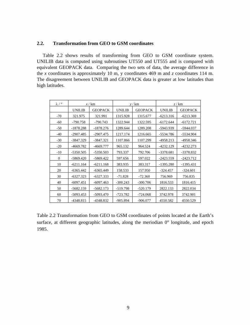
2.2. Transformation from GEO to GSM coordinates Table 2.2 shows results of transforming from GEO to GSM coordinate system.

UNILIB data is computed using subroutines UT550 and UT555 and is compared with equivalent GEOPACK data. Comparing the two sets of data, the average difference in the x coordinates is approximately 10 m, y coordinates 469 m and z coordinates 114 m. The disagreement between UNILIB and GEOPACK data is greater at low latitudes than high latitudes.

λ / ° x / km y / km z / km UNILIB GEOPACK UNILIB GEOPACK UNILIB GEOPACK

-70 321.975 321.991 1315.928 1315.677 -6213.316 -6213.369 -60 -790.758 -790.743 1322.944 1322.595 -6172.644 -6172.721 -50 -1878.288 -1878.276 1289.644 1289.208 -5943.939 -5944.037 -40 -2907.485 -2907.475 1217.174 1216.665 -5534.786 -5534.904 -30 -3847.329 -3847.321 1107.866 1107.299 -4958.213 -4958.346 -20 -4669.782 -4669.777 965.132 964.524 -4232.129 -4232.273 -10 -5350.505 -5350.503 793.337 792.706 -3378.681 -3378.832 0 -5869.420 -5869.422 597.656 597.022 -2423.559 -2423.712 10 -6211.164 -6211.168 383.935 383.317 -1395.280 -1395.431 20 -6365.442 -6365.449 158.533 157.950 -324.457 -324.601 30 -6327.323 -6327.333 -71.828 -72.360 756.969 756.835 40 -6097.451 -6097.463 -300.243 -300.706 1816.533 1816.415 50 -5682.159 -5682.173 -519.798 -520.179 2822.133 2822.034 60 -5093.453 -5093.470 -723.782 -724.068 3742.978 3742.901 70 -4348.815 -4348.832 -905.894 -906.077 4550.582 4550.529

Table 2.2 Transformation from GEO to GSM coordinates of points located at the Earth’s surface, at different geographic latitudes, along the meriodian 0° longitude, and epoch 1985.

9

2.3. Transformation from GEO to MAG coordinates Table 2.3 shows the results of transforming from GEO to MAG coordinate system.

The UNILIB and GEOPACK data are in excellent agreement. The average difference in the x coordinates is 9 m and in the y and z coordinates 4 m.

λ / ° x / km y / km z / km UNILIB GEOPACK UNILIB GEOPACK UNILIB GEOPACK

-70 1844.816 1844.816 2067.435 2067.434 -5723.897 -5723.897 -60 2079.018 2079.004 3021.035 3021.037 -5198.851 -5198.854 -50 2249.641 2249.626 3881.637 3881.640 -4515.924 -4515.928 -40 2351.677 2351.663 4623.258 4623.260 -3696.478 -3696.483 -30 2382.267 2382.253 5223.806 5223.810 -2765.835 -2765.840 -20 2340.716 2340.702 5665.635 5665.639 -1752.394 -1752.401 -10 2228.457 2228.444 5935.919 5935.923 -686.742 -686.748 0 2048.961 2048.950 6026.882 6026.886 399.227 399.222 10 1807.616 1807.607 5935.919 5935.923 1473.146 1473.141 20 1511.581 1511.573 5665.635 5665.640 2502.991 2502.986 30 1169.612 1169.606 5223.806 5223.810 3457.896 3457.892 40 791.864 791.861 4623.258 4623.261 4308.977 4308.974 50 389.643 389.642 3881.637 3881.640 5030.172 5030.169 60 -24.893 -24.891 3021.035 3021.037 5599.084 5599.083 70 -439.083 -439.079 2067.435 2067.436 5997.796 5997.795

Table 2.3 Transformation from GEO to MAG coordinates of points located at the Earth’s surface, at different geographic latitudes, along the meriodian 0° longitude, and epoch 1985.

10

2.4. Transformation from GSM to GSE coordinates Table 2.4 shows the results of transforming from GSM to GSE coordinate system. As

UNILIB works in the GEO coordinate system, a GSM to GSE transformation requires subroutine UT555 to preform an initial transformation from GEO to GSM. Comparing UNILIB with GEOPACK data, the x and z coordinates are in excellent agreement with average differences of 10 m and 17 m respectively. A relatively large disagreement of 399 m is seen between the y coordinate data (this is expected as the results of Table 2.2 show that the initial transformation of GEO to GSM has an average difference in the y coordinates of 469 m, limiting the accuracy of the GSM to GSE transformation).

λ / ° x / km y / km z / km

UNILIB GEOPACK UNILIB GEOPACK UNILIB GEOPACK -70 321.975 321.993 -468.862 -468.803 -6333.809 -6333.812 -60 -790.758 -790.743 -450.783 -450.826 -6296.706 -6296.705 -50 -1878.288 -1878.275 -418.987 -419.132 -6067.787 -6067.781 -40 -2907.486 -2907.474 -374.490 -374.731 -5654.656 -5654.645 -30 -3847.329 -3847.321 -318.683 -319.013 -5070.472 -5070.458 -20 -4669.782 -4669.777 -253.286 -253.694 -4333.387 -4333.369 -10 -5350.505 -5350.503 -180.282 -180.757 -3465.886 -3465.864 0 -5869.421 -5869.422 -101.864 -102.391 -2494.084 -2494.060 10 -6211.164 -6211.168 -20.370 -20.934 -1446.996 -1446.971 20 -6365.442 -6365.450 61.770 61.187 -355.794 -355.768 30 -6327.324 -6327.334 142.103 141.518 746.973 746.999 40 -6097.451 -6097.463 218.209 217.641 1828.202 1828.228 50 -5682.159 -5682.173 287.776 287.241 2855.138 2855.163 60 -5093.454 -5093.470 348.663 348.178 3796.338 3796.360 70 -4348.815 -4348.832 398.976 398.556 4622.690 4622.710

Table 2.4 Transformation from GSM to GSE coordinates of points located at the Earth’s surface, at different geographic latitudes, along the meriodian 0° longitude, and epoch 1985.

11

2.5. Transformation from MAG to SM coordinates Table 2.5 shows the results of transforming from MAG to SM coordinate system,

again requiring UNILIB to preform an initial transformation from GEO to MAG. As with the GSM to GSE transformation, the x and z coordinates are in very good agreement with average differences of 76 and 4 m respectively, while the y coordinates disagree quite appreciably with an average disagreement of 467 m (the disagreement being greater at low latitudes than high latitudes).

λ / ° x / km y / km z / km

UNILIB GEOPACK UNILIB GEOPACK UNILIB GEOPACK -70 -2438.435 -2438.563 1315.928 1315.689 -5723.897 -5723.897 -60 -3420.349 -3420.477 1322.944 1322.595 -5198.851 -5198.854 -50 -4297.070 -4297.195 1289.644 1289.208 -4515.924 -4515.928 -40 -5042.161 -5042.279 1217.174 1216.665 -3696.478 -3696.483 -30 -5633.469 -5633.577 1107.866 1107.299 -2765.835 -2765.840 -20 -6053.668 -6053.762 965.133 964.524 -1752.394 -1752.401 -10 -6290.610 -6290.688 793.337 792.706 -686.742 -686.748 0 -6337.535 -6337.594 597.656 597.022 399.227 399.222 10 -6193.158 -6193.197 383.935 383.317 1473.146 1473.141 20 -5861.669 -5861.687 158.533 157.950 2502.991 2502.986 30 -5352.661 -5352.656 -71.828 -72.360 3457.896 3457.892 40 -4680.963 -4680.935 -300.243 -300.706 4308.977 4308.974 50 -3866.360 -3866.311 -519.798 -520.179 5030.172 5030.169 60 -2933.157 -2933.088 -723.782 -724.068 5599.084 5599.083 70 -1909.565 -1909.478 -905.894 -906.077 5997.796 5997.795

Table 2.5 Transformation from MAG to SM coordinates of points located at the Earth’s surface, at different geographic latitudes, along the meriodian 0° longitude, and epoch 1985.

12

2.6. Transformation from GEO to GEI coordinates Since the GEO and GEI coordinate systems have their z-axis in common [4] (parallel

to the Earth’s rotation axis), the transformation from GEO to GEI is easily implemented by UNILIB as it simply requires a rotation about the z-axis.

2.7. Modified Julian Day Astronomers who need to deal with events separated by large time spans use ‘Julian

Day’ to refer to time. The Julian Day is the number of days that has elapsed since noon, 1st of January, 4713 BC. The modified Julian Day (MDJ), as defined by Scaliger, began at midnight, November 17, 1858. A second version of MDJ, as defined by Klinkard, began at midday, 1st of January, 1950. The difference between the starting times of the two versions of MJD is 33282.5 days.

UNILIB subroutine UT540 (compute modified Julian Day from date) converts an

‘actual’ date into MJD (Klinkard version). Accurate evaluation of MJD within UNILIB is of great importance, as it is required, for example, to evaluate the geomagnetic field, for coordinate systems such as SM or GSE which are dependent on the suns position.

Table 2.6 shows results of converting two actual dates (column 1) into MJD

(Klinkard) using subroutine UT540 (column 2). The results of converting the dates to MJD (Scaliger) are shown in column 3. For each of the dates the difference between MJD (Klinkard) and MJD (Scalinger) is, as expected, 33282.5 days (column 4), indicating that subroutine UT540 accurately calculates modified Julian Day.

Subroutine UT545 (compute date from modified Julian Day) performs the reverse

transformation from MJD (Klinkard) into the date. Applying this transformation to the column 2 data returned the initial dates of column 1.

Date MDJ (Klinkard) MDJ (Scaliger) Difference 1/1/1985 12784 46066.5 33282.5 5/1/1999 18017 51299.5 33282.5

Table 2.6 Calculation of the Klinkard and Scalinger versions of modified Julian Day (MJD) from a given date.

13

2.8. Recommendations UNILIB subroutines UT550 (select a coordinate transformation) and UT555

(coordinate conversion) implement the transformation from one coordinate system to another. Using these subroutines, the transformations GEO to MAG and GEO to GEI (a simple rotation about the z-axis) are accurately implemented. For transformations involving GEO to GSM, GSM to GSE and MAG to SM, the final y coordinate positions disagree by an average of 400 to 450 m with equivalent GEOPACK data. Additionally, the disagreement is greater at low latitudes than at high latitudes. The x and z positions were much more reliably found, typically disagreeing by tens of meters.

A possible recommendation is that the relative inaccuracy of the y coordinate positions

involving these transformations is examined further. This could be done by finding a second method with which to compare UNILIB results and so determine which of either GEOPACK or UNILIB is the ‘most’ correct.

14

3. Evaluation of the geomagnetic field vector B The Earth’s internal magnetic field (geomagnetic field) results primarily from

convective motion of the core and is approximately dipole configuration. The effective dipole is centered around 500 km from the center of the Earth toward the western Pacific and inclined at an angle of about 11.2° from the axis of rotation. The Earth’s external field comes from currents flowing above the surface of the Earth and is much less stable than the internal field [5].

In the UNILIB library, the magnetic field model of the Earth is defined by selection of

an internal field model using subroutine UM510 (select a geomagnetic field model) and an external field model using subroutine UM520 (select an external magnetic field model). These subroutines modify the contents of common block UC140 (magnetic field description) which is used by subroutine UM530 (evaluate the magnetic field vector) to evaluate the magnetic field at any geographic location. The most commonly used geomagnetic field model is the IGRF model, while for the external field it is Tsyganenko’s model [6]. (In the UNILIB library (version 2.03), see Example 1 (page 79) for a sample program for evaluation of the magnetic field vector and frequently asked questions number T.03 (page 38) on how to customize the magnetic field model.)

The IGRF model is the empirical representation of the Earth’s magnetic field. The

model employs a spherical harmonics expansion of the scalar potential VM giving

[ ]∑ ∑∞

= =

+

+⎟⎠⎞

⎜⎝⎛=

0 0

1

)sin()cos()(cosReRen

n

m

mn

mn

mn

n

M mhmgPr

V φφθ (3.1)

where r is the distance from the center of the Earth, θ and φ are the geographic

colatitude and east longitude respectively, Re is the Earth radius (6371.2 km), PP

mn (cos θ)

are normalized associated Legendre functions and gnm and hn

m gaussian coefficients. As both the center of the dipole and its inclination changes every year, the IGRF model consists of coefficient sets for the epochs 1945 to 1995 in steps of 5 years.

3.1. Centered dipole model Within a few Earth radii the magnetic field of the Earth is similar to the field found if

the Earth was modelled as a centered and aligned dipole (the dipole is aligned with the Earth’s axis of rotation). The fields from this dipole may be represented by exact analytical formulas [7].

15

The strength of a dipole magnetic field is given by

λλ 23 sin31),( +=

rMrB

(3.2) where λ is the latitude, r the distance from the center of the Earth and M the Earth’s

dipole moment. The field components, in spherical coordinates, are given as

λsin23rMBr −=

(3.3)

λθ cos3rMB −=

(3.4)

and

0=φB (3.5)

The field B along a field line can be shown to be

λ

λλcos

²sin31Re),( 6

3

00

+⎟⎟⎠

⎞⎜⎜⎝

⎛=

rMrB

(3.6)

where ro is the radius at the equator. Through subroutine UM510, UNILIB allows the centered dipole model (obtained

from the IGRF model by truncation to the 2nd order of the gaussian coefficients) to be selected. Table 3.1 shows modulus values of B computed using UNILIB subroutine UM530 and modulus values computed using equation (3.6) [labelled UNILIB and Exact respectively] at positions of radius 1 Re (on the Earth’s surface) and 3 Re and for the year 1985 (the magnetic field is year dependent with M= 0.3043476883 Gauss for 1985). The UNILIB field values, for both 1 Re and 3 Re, match the exact field values to the 14 digits shown. [Only data for latitudes 0° to 70° are shown as the fields are symmetrical about the equator.]

16

λ / ° 1 Re | B | / nT 3 Re | B | / nT

UNILIB Exact UNILIB Exact 0 30434.7688343447 30434.7688343447 1127.2136605313 1127.2136605313 10 31781.5511649967 31781.5511649967 1177.0944875925 1177.0944875925 20 35374.2276695716 35374.2276695716 1310.1565803545 1310.1565803545 30 40261.4147727076 40261.4147727076 1491.1635101003 1491.1635101003 40 45545.7890066098 45545.7890066098 1686.8810743189 1686.8810743189 50 50566.3610888245 50566.3610888245 1872.8281884750 1872.8281884750 60 54867.0597945616 54867.0597945616 2032.1133257245 2032.1133257245 70 58138.1095907092 58138.1095907092 2153.2633181744 2153.2633181744

Table 3.1 Comparison of UNILIB and ‘exact’ modulus values of magnetic field, computed using the centered dipole model, at points located at different geographic latitudes, at a radius of 1 and 3 Re, and epoch 1985.

Table 3.2 shows BBr field values (for 1985) computed using subroutine UM530 and

equation (3.3) [again labelled UNILIB and Exact respectively]. Again, the UNILIB field values, at both 1 Re and 3 Re, match the exact field values to the number of digits shown.

λ / ° 1 Re BBr / nT 3 Re BBr / nT

UNILIB Exact UNILIB Exact 0 0.000000000 0.000000000 0.0000000000 0.000000000 10 -10569.8842915960 -10569.8842915960 -391.477195985 -391.477195985 20 -20818.6079976120 -20818.6079976120 -771.059555467 -771.059555467 30 -30434.7688343450 -30434.7688343450 -1127.213660531 -1127.213660531 40 -39126.1846207820 -39126.1846207820 -1449.117948918 -1449.117948918 50 -46628.7710863210 -46628.7710863210 -1726.991521716 -1726.991521716 60 -52714.5659376990 -52714.5659376990 -1952.391331026 -1952.391331026 70 -57198.6553779170 -57198.6553779170 -2118.468717701 -2118.468717701

Table 3.2 Comparison of UNILIB and ‘exact’ BBr field values, computed using the centered dipole model, at points located at different geographic latitudes, at a radius of 1 and 3 Re, and epoch 1985.

17

Table 3.3 shows BBθ field values (for 1985) computed using subroutine UM530 and equation (3.4). Again, both sets of field values match to the number of digits shown.

λ / ° 1 Re BBθ / nT 3 Re BBθ / nT

UNILIB Exact UNILIB Exact 0 -30434.7688343450 -30434.7688343450 -1127.2136605313 -1127.2136605313 10 -29972.3963091970 -29972.3963091970 -1110.0887521925 -1110.0887521925 20 -28599.3276889590 -28599.3276889590 -1059.2343588503 -1059.2343588503 30 -26357.2829688490 -26357.2829688490 -976.1956655129 -976.1956655129 40 -23314.3855431600 -23314.3855431600 -863.4957608578 -863.4957608578 50 -19563.0923103910 -19563.0923103910 -724.5589744589 -724.5589744589 60 -15217.3844171720 -15217.3844171720 -563.6068302656 -563.6068302656 70 -10409.3039988060 -10409.3039988060 -385.5297777336 -385.5297777336

Table 3.3 Comparison of UNILIB and ‘exact’ BBθ field values, computed using the centered dipole model, at points located at different geographic latitudes, at a radius of 1 and 3 Re, and epoch 1985.

The magnetic field strength of a centered dipole is independent of longitude. This was

checked within the UNILIB subroutine by calculating the magnetic field on the Earth’s surface, at the equator, for epoch 1985, as a function of longitude. Table 3.4 shows that the field strengths computed by subroutine UM530 are, as expected, independent of longitude. Similar results were found for latitudes of 30° and –30°.

Longitude / ° | B | / nT

360 30434.7688343447 280 30434.7688343447 200 30434.7688343447 120 30434.7688343447 80 30434.7688343447 0 30434.7688343447

Table 3.4 Variation of magnetic field with longitude, computed using UNILIB’s implementation of the centered dipole model, at points located at 0° latitude, at a radius of 1 Re, and epoch 1985.

18

3.2. IGRF model A more representative model of the Earth’s internal field is the IGRF model [5].

Table 3.5 shows geomagnetic field values computed using UNILIB’s implementation of the IGRF model compared with results computed using GEOPACK’s implementation. The table shows modulus values and field component values in spherical coordinates, calculated at 3 Re, 320° longitude and epoch 1985. The UNILIB and GEOPACK field values either agree to all digits shown or differ by ‘one’ point in the final digit. [By choosing the longitude as 320°, the comparisons were made in the unfavorable region of the South Atlantic Anomaly.]

λ / ° | B | / nT Br / nT BBθ / nT BBφ / nT

UNILIB GEOPACK UNILIB GEOPACK UNILIB GEOPACK UNILIB GEOPACK -80 2032.181 2032.183 1980.517 1980.518 -446.370 -446.370 -89.833 -89.833 -70 1884.150 1884.150 1787.311 1787.311 -588.421 -588.421 -96.445 -96.445 -60 1713.688 1713.688 1556.739 1556.74 -708.670 -708.670 -105.242 -105.242 -50 1532.643 1532.643 1296.742 1296.742 -808.769 -808.769 -115.528 -115.528 -40 1354.673 1354.673 1012.832 1012.832 -890.692 -890.692 -126.410 -126.410 -30 1197.399 1197.399 708.462 708.462 -955.560 -955.560 -136.937 -136.937 -20 1084.553 1084.554 386.158 386.158 -1002.879 -1002.880 -146.224 -146.225 -10 1042.918 1042.918 48.991 48.991 -1030.390 -1030.390 -153.547 -153.547 0 1088.328 1088.329 -298.130 -298.130 -1034.640 -1034.640 -158.401 -158.401 10 1212.177 1212.178 -647.758 -647.758 -1011.940 -1011.940 -160.535 -160.535 20 1387.833 1387.834 -989.976 -989.976 -959.402 -959.402 -159.936 -159.936 30 1586.242 1586.242 -1313.179 -1313.177 -875.872 -875.872 -156.774 -156.774 40 1783.488 1783.489 -1605.270 -1605.269 -762.262 -762.262 -151.332 -151.332 50 1961.535 1961.535 -1854.909 -1854.908 -621.464 -621.464 -143.941 -143.941 60 2107.222 2107.222 -2052.453 -2052.453 -457.828 -457.828 -134.970 -134.970 70 2211.302 2211.301 -2190.391 -2190.393 -276.489 -276.489 -124.852 -124.852 80 2267.677 2267.678 -2263.290 -2263.290 -82.818 -82.818 -114.128 -114.128

Table 3.5 Comparison of UNILIB and GEOPACK magnetic field values, computed using the IGRF model, at points located at different geographic latitudes, at a radius of 3 Re, along the meriodian 320° longitude, and epoch 1985.

A second comparison can be made by comparing magnetic field strengths computed

using BILCAL’s [3] implementation of the IGRF model. Table 3.6 shows field values computed using UNILIB and BILCAL, at positions of 1 Re, 320° longitude and for

19

epoch 1985. The UNILIB and BILCAL field values match to the number of digits shown. [As BILCAL’s field components are in geodetic coordinates, while UNILIB’s are in geocentric, results are shown as geodetic field components.]

λ / ° | B | / nT BBr / nT Bθ / nT Bφ / nT UNILIB BILCAL UNILIB BILCAL UNILIB BILCAL UNILIB BILCAL

-80 49740.3 49740.3 -19209.2 -19209.2 3193.9 3193.9 45770.0 45770.1 -70 41657.2 41657.2 -20402.9 -20402.9 1682.2 1682.2 36279.7 36279.7 -60 33902.9 33902.9 -19396.9 -19396.9 -484.2 -484.2 27801.7 27801.7 -50 28116.0 28116.0 -17462.1 -17462.1 -2716.5 -2716.5 21867.9 21867.9 -40 25023.6 25023.6 -16420.4 -16420.4 -4656.9 -4656.9 18299.3 18299.3 -30 23979.5 23979.5 -17168.9 -17168.9 -6289.9 -6289.9 15514.0 15514.0 -20 24150.9 24150.9 -19507.5 -19507.5 -7764.3 -7764.3 11934.8 11934.8 -10 25355.7 25355.7 -22776.2 -22776.2 -9036.5 -9036.5 6519.2 6519.2 0 27790.7 27790.7 -25987.1 -25987.1 -9767.2 -9767.2 -1261.5 -1261.5 10 31562.1 31562.1 -27927.3 -27927.3 -9684.1 -9684.1 -11065.8 -11065.8 20 36406.1 36406.1 -27843.0 -27843.0 -8977.3 -8977.3 -21669.8 -21669.8 30 41758.8 41758.9 -25798.1 -25798.1 -8174.1 -8174.1 -31803.2 -31803.2 40 46939.8 46939.8 -22157.0 -22157.0 -7628.9 -7628.9 -40672.1 -40672.1 50 51128.3 51128.3 -17261.3 -17261.3 -7261.5 -7261.5 -47575.4 -47575.4 60 53628.9 53628.9 -11867.8 -11867.8 -6761.2 -6761.2 -51860.4 -51860.4 70 54597.7 54597.7 -7173.8 -7173.8 -5849.4 -5849.4 -53807.3 -53807.3 80 55221.5 55221.5 -3733.5 -3733.5 -4331.6 -4331.6 -54924.6 -54924.6

Table 3.6 Comparison of UNILIB and BILCAL magnetic field values, computed using the IGRF model, at points located at different geographic latitudes, at a radius of 1 Re, along the meriodian 320° longitude, and epoch 1985.

3.2.1. Computation time

The computer evaluation time of the UNILIB subroutines used to evaluate B field values is very rapid. For the IGRF model, using a Hewlett-Packard Workstation, it took 1.3 seconds to evaluate 100 B field values.

20

3.3. Tsyganenko’s external magnetic field model

Table 3.7 shows field values, in cartesian coordinates, computed using UNILIB’s implementation of the Tsyganenko (1989c) external field model [6] [subroutine UM520 (select an external magnetic field model)] compared with results computed using GEOPACK’s implementation. As GEOPACK uses a cartesian Geocentric Solar Magnetospheric (GSM) coordinate system, while UNILIB calculates in spherical GEO, UNILIB results were transformed into cartesian GSM for comparison [subroutine UT556 (vector conversion) and UT542 (convert spherical vector components to cartesian components)]. Additionally, as UNILIB only allows evaluation of either the internal magnetic field or the total magnetic field (i.e. internal + external), the external field was computed by subtracting the internal field from the total field.

λ / ° | B | / nT Bx / nT By / nT Bz / nT UNILIB GEOPACK UNILIB GEOPACK UNILIB GEOPACK UNILIB GEOPACK

0 43.82007 43.82012 1.33399 1.33576 -8.20702 -8.20681 -43.024 -43.02403 5 43.92521 43.92484 0.87812 0.87971 -8.22648 -8.22629 -43.13895 -43.13867 10 43.96019 43.96037 0.43223 0.43345 -8.22381 -8.22365 -43.1819 -43.18214 15 43.92680 43.92762 0.00774 0.00948 -8.19969 -8.19955 -43.15483 -43.15556 20 43.82881 43.82873 -0.38307 -0.38113 -8.15553 -8.15542 -43.06155 -43.0616 25 43.66750 43.66715 -0.73127 -0.72923 -8.09336 -8.09325 -42.90477 -42.90435 30 43.44738 43.44722 -1.03047 -1.0279 -8.01564 -8.01556 -42.68907 -42.68904 35 43.17429 43.17440 -1.27369 -1.27301 -7.92516 -7.92509 -42.42159 -42.4217 40 42.85468 42.85466 -1.46425 -1.46231 -7.82481 -7.82475 -42.10877 -42.10886 45 42.49443 42.49445 -1.59760 -1.59615 -7.71746 -7.71741 -41.75731 -41.75731 50 42.10103 42.10044 -1.67770 -1.67638 -7.60586 -7.60581 -41.37428 -41.37376 55 41.67903 41.67929 -1.70823 -1.70641 -7.49254 -7.49249 -40.96454 -40.96479 60 41.23735 41.23752 -1.69267 -1.69065 -7.37976 -7.37972 -40.53645 -40.53658 65 40.78083 40.7813 -1.63527 -1.63423 -7.26950 -7.26946 -40.09443 -40.09487 70 40.3165 40.31641 -1.54427 -1.54271 -7.16344 -7.16340 -39.64501 -39.64491 75 39.84765 39.84812 -1.42322 -1.42191 -7.06297 -7.06293 -39.19086 -39.1914 80 39.38149 39.38113 -1.27955 -1.27769 -6.96919 -6.96915 -38.73866 -38.73851

Table 3.7 Comparison of UNILIB and GEOPACK external magnetic field values, computed using the Tsyganenko (1989c) model, at points located at different geographic latitudes, at a radius of 1 Re, and along the meriodian 0° longitude.

21

Table 3.7 shows modulus values and field component values, calculated at 1 Re, 0° longitude, and using UNILIB’s default parameter values of Kp, Dst, solar wind velocity, etc. Typically, the modulus values agree to the first 4 or 5 digits, values of BBx to 3 digits and values of ByB and BBz to 4 or 5 digits. The good agreement of the results provides not only verification of UNILIB’s implementation of the Tsyganenko (1989c) external field model and the calculation of the geomagnetic field but also the implementation of the vector component conversion subroutine UT556 (vector conversion).

3.3.1. Computation time

The computer evaluation time for the evaluation of B field values using Tsyganenko’s external field model were similar to those for the IGRF model. Again, using a Hewlett-Packard Workstation, 100 B field values were evaluated in 1.3 seconds.

3.4. Recommendations UNILIB’s implementation of the centered dipole model, the IGRF model,

Tsyganenko´s (1989c) model, and the resulting calculation of the geomagnetic field, has been validated.

22

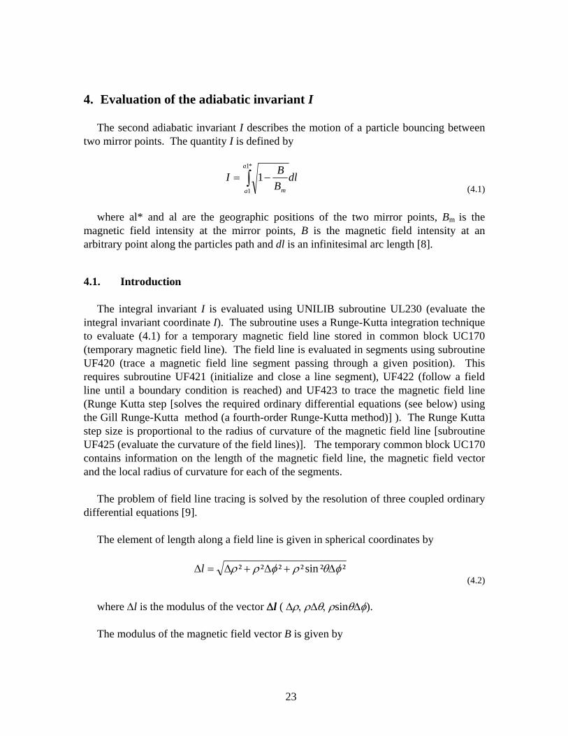
4. Evaluation of the adiabatic invariant I The second adiabatic invariant I describes the motion of a particle bouncing between

two mirror points. The quantity I is defined by

dlBBI

a

a m∫ −=

*1

1

1 (4.1)

where al* and al are the geographic positions of the two mirror points, BBm is the

magnetic field intensity at the mirror points, B is the magnetic field intensity at an arbitrary point along the particles path and dl is an infinitesimal arc length [8].

4.1. Introduction The integral invariant I is evaluated using UNILIB subroutine UL230 (evaluate the

integral invariant coordinate I). The subroutine uses a Runge-Kutta integration technique to evaluate (4.1) for a temporary magnetic field line stored in common block UC170 (temporary magnetic field line). The field line is evaluated in segments using subroutine UF420 (trace a magnetic field line segment passing through a given position). This requires subroutine UF421 (initialize and close a line segment), UF422 (follow a field line until a boundary condition is reached) and UF423 to trace the magnetic field line (Runge Kutta step [solves the required ordinary differential equations (see below) using the Gill Runge-Kutta method (a fourth-order Runge-Kutta method)] ). The Runge Kutta step size is proportional to the radius of curvature of the magnetic field line [subroutine UF425 (evaluate the curvature of the field lines)]. The temporary common block UC170 contains information on the length of the magnetic field line, the magnetic field vector and the local radius of curvature for each of the segments.

The problem of field line tracing is solved by the resolution of three coupled ordinary

differential equations [9]. The element of length along a field line is given in spherical coordinates by

²²sin²²²² φθρφρρ Δ+Δ+Δ=Δl (4.2)

where Δl is the modulus of the vector Δl ( Δρ, ρΔθ, ρsinθΔφ).

The modulus of the magnetic field vector B is given by

23

222φθρ BBB ++

(4.3) The unit vectors of both quantities follow as

lll ΔΔ

ΔΔ

ΔΔ ϕθρθρρ sin,,

(4.4)

and

BB

BB

BB φθρ ,,

(4.5) Since the vector Δl is always tangential to the field line, the two unit vectors must be

equal everywhere along the field line. This produces a set of three ordinary differential equations which, in spherical coordinates, are

lB

BΔ=Δ ρρ

(4.6)

ρθ θ l

BB Δ

=Δ (4.7)

and

θρφ φ

sinl

BB Δ

=Δ (4.8)

Given B, BBρ, BθB and BBφ, the differential equations can be solved by a Runge-Kutta

method (subroutine UF423) to find the increments Δρ, Δθ and Δφ, allowing the field line to be traced.

24

4.2. Calculation of I for a centered dipole model For the centered dipole model, the integral invariant I at magnetic latitude λ on a line

of force having an equatorial radial distance ro is given by [8]

( )∫ +⎥⎥⎦

⎤

⎢⎢⎣

⎡⎟⎟⎠

⎞⎜⎜⎝

⎛−−

⎟⎟⎠

⎞⎜⎜⎝

⎛++

−=Y

aaa

a dYYYY

YY

rI0

2/12

2/13

2

22/1

2

2

0 3111

3131

12 (4.9)

where Y= sin λ. I values computed using this integral will be referred to as ‘exact’ (the listing of the

Fortran program is given in Appendix A1). Table 4.1 shows I computed by UNILIB and ‘exact’ values computed using (4.9) for 1

Re and 3 Re. The columns labeled ‘Error’ show the relative error defined as( | UNILIB estimate – Exact | / Exact ). The two sets of results are in good agreement with a relative error of between 10-5 at low latitudes to 10-6 at high latitudes. Note that since the value of I increases with latitude, the relative error remains small.

1 Re I / km 3 Re I / km

λ / ° UNILIB / km Exact / km Error UNILIB / km Exact / km Error

-70 133811.361 133811.625 1.98E-06 161258.896 401434.875 5.98E-01 -60 53753.269 53753.578 5.75E-06 161258.896 161260.734 1.14E-05 -50 25877.046 25877.268 8.58E-06 77630.588 77631.805 1.57E-05 -40 13145.706 13146.062 2.71E-05 39436.781 39438.188 3.57E-05 -30 6436.064 6436.187 1.91E-05 19308.025 19308.561 2.78E-05 -20 2664.257 2664.337 3.00E-05 7992.653 7993.011 4.49E-05 -10 649.371 649.420 7.55E-05 1948.114 1948.261 7.55E-05 0 0.000 0.000 0.0 0.000 0.000 0.0 10 649.372 649.420 7.39E-05 1948.115 1948.261 7.50E-05 20 2664.258 2664.337 2.97E-05 7992.653 7993.011 4.48E-05 30 6436.064 6436.187 1.91E-05 19308.025 19308.561 2.77E-05 40 13145.707 13146.062 2.70E-05 39436.782 39438.188 3.56E-05 50 25877.046 25877.268 8.58E-06 77630.589 77631.805 1.57E-05 60 53753.269 53753.578 5.75E-06 161258.897 161260.734 1.14E-05 70 133811.361 133811.625 1.97E-06 161258.896 401434.875 5.98E-01

Table 4.1 Comparison of UNILIB and ‘exact’ I values, computed using the centered dipole model, at points located at different geographic latitudes, and at a radius of 1 and 3 Re.

25

The UNILIB estimate at ±70° and 3 Re is unreliable (equal to the estimate at ±60°).

For high latitudes the magnetic field lines penetrate out of the magnetosphere and into the magnetotail. By default UNILIB prevents the field line from being traced out of the magnetosphere, stopping the calculation of I within a fixed radial distance,. This explains the ‘saturation’ for the UNILIB estimate at λ=±70° as the field line in this case is incompletely traced.

Parameters kum533 in common block UC190 (control parameters, set 1) and xbmin in common block UC192 (control parameters, set 2) control whether the field lines are traced outside of the magnetosphere. Parameter kum533 is set by default to ‘1’ and prevents the magnetic field being traced outside the magnetosphere [subroutine UM533 (distance to magnetosphere)]. Parameter xbmin, the lowest allowed value of the magnetic field intensity, is set by default to 4.0E-05 Gauss. When kum533 is set to less than zero allowing field lines to be traced outside the magnetosphere and xbmin set to a lower intensity, say 1.0E-07 Gauss, the UNILIB estimate at ±70° and 3 Re was accurate (relative error approximately 10-5).

4.3. Calculation of I for the IGRF model As (4.9) is valid only for a centered dipole model, an alternative and independent

method of computing I (i.e. an alternative method of tracing the magnetic field line) which can be applied to the IGRF model had to be developed first. The ‘best’ alternative method was found through examination of the centered dipole model.

4.3.1. Comparison of integration methods Four ‘Runge-Kutta’ methods were examined to solve the differential equations (4.6) to

(4.8); Euler, Runge-Kutta (as used by UNILIB), Gill and Runge-Kutta adaptive [9]. The first three methods require a constant step size during integration. The fourth method, Runge-Kutta adaptive, exerts adaptive control over the step size. Each of the methods was applied in a Fortran program to evaluate I for the centered dipole model. As the field line is traced the value of the integrand √(1-B/BBm) and the length of the line segment is stored in a vector. Using this information, integral (4.1) is evaluated using the CERN integration routine DGAUSS [10].

Table 4.2 shows values of I, computed using the four Runge-Kutta methods, at a

radius of 3 Re for the centered dipole model. The final column of the table shows, for comparison, ‘exact’ values of I computed using (4.9). The step size used by the Euler method is 0.7 km, for Runge-Kutta 0.7 km, for Gill 15 km and for Runge-Kutta adaptive, an initial step size of 0.4 km.

26

The maximum difference between I computed using the Euler method to trace the

field line and exact values is 1.26 km (average difference 0.69 km). The two sets of data agree better at low rather than high latitudes. Additionally, Euler values are symmetric, as are the exact values, about 0°.

The maximum difference between I computed using the Runge-Kutta method and

exact values is 7.99 km (average difference1.69 km). Again the two sets of data agree better at low rather than high latitudes. Additionally, Runge-Kutta values agree better at northern hemisphere latitudes than southern hemisphere latitudes. Neglecting the Runge-Kutta values for ±70° , which are significantly different from the exact values, the average difference between the two sets of data is 0.91 km.

The maximum difference between I computed using the Gill method and exact values

is 0.8 km (average difference 0.50 km). The two sets of data agree better at low latitudes and in the Northern hemisphere.

The maximum difference between I computed using the Runge-Kutta adaptive method

and exact values is 2.38 km (average difference 0.47 km). Again, the two sets of data agree better at low latitudes and in the Northern hemisphere.

λ / ° Euler / km Runge-Kutta /

km Gill / km Runge-Kutta

adaptive / km Exact / km

-70 401433.613 401440.330 401434.058 401436.333 401434.875 -60 161261.296 161263.764 161260.160 161261.573 161260.734 -50 77632.741 77633.768 77631.206 77632.337 77631.805 -40 39439.087 39439.518 39437.578 39438.538 39438.188 -30 19309.320 19309.472 19307.963 19308.810 19308.561 -20 7993.529 7993.563 7992.458 7993.159 7993.011 -10 1948.500 1948.499 1947.813 1948.308 1948.261 0 0.000 0.000 0.000 0.000 0.000 10 1948.500 1948.499 1947.995 1948.308 1948.261 20 7993.529 7993.492 7992.646 7993.138 7993.011 30 19309.320 19309.165 19308.130 19308.722 19308.561 40 39439.090 39438.657 39437.676 39438.291 39438.188 50 77632.743 77631.687 77631.316 77631.742 77631.805 60 161261.310 161258.822 161260.195 161260.161 161260.734 70 401433.617 401426.888 401434.145 401432.492 401434.875

Table 4.2 Comparison of different integration methods applied to evaluate I, compared with ‘exact’ values, computed using the centered dipole model, at points located at different geographic latitudes, and at a radius of 3 Re.

27

Its is concluded that Gill and Runge-Kutta adaptive are the most suitable for

evaluating I. Section 4.3.2 will apply the Runge-Kutta adaptive program to evaluate I for the IGRF model and compare with the equivalent UNILIB data.

4.3.2. Results Table 4.3 shows I computed using UNILIB and the Runge-Kutta adaptive (RK

adaptive) program (the listing of the Fortran program is given in Appendix A2) for the 1985 IGRF model at 1 and 3 Re and 0° longitude. The columns labeled ‘Error’ show the relative error defined as ( | UNILIB estimate – RK adaptive estimate | / RK adaptive estimate). The two sets of data have a relative error of between 10-3 at low latitudes to 10-4 at high latitudes (two orders of magnitude greater than the relative errors shown for the centered dipole model). Additionally, as discussed in section 4.2, saturation is seen for the UNILIB estimate of I at +70° latitude and radius 3 Re.

λ / ° I Re I / km 3 Re I / km

UNILIB RK adaptive Error UNILIB RK adaptve Error -70 54790.651 54796.757 1.11E-04 213668.369 213696.916 1.34E-04 -60 33714.655 33719.567 1.46E-04 108432.565 108448.406 1.46E-04 -50 21912.759 21918.216 2.49E-04 58494.753 58520.259 4.36E-04 -40 14365.312 14371.110 4.03E-04 31606.675 31628.864 7.02E-04 -30 9078.048 9081.953 4.30E-04 15925.285 15940.199 9.36E-04 -20 5145.352 5148.855 6.80E-04 6540.867 6557.312 2.51E-03 -10 2284.202 2288.798 2.01E-03 1443.546 1452.069 5.87E-03 0 527.825 529.856 3.83E-03 19.989 20.614 3.03E-02 10 7.833 8.081 3.07E-03 2264.042 2278.234 6.23E-03 20 892.508 894.830 2.60E-03 8565.012 8578.372 1.56E-03 30 3589.598 3593.310 1.03E-03 20260.057 20277.488 8.60E-04 40 9477.023 9481.242 4.45E-04 41137.869 41155.962 4.40E-04 50 22032.144 22035.695 1.61E-04 80792.669 80813.728 2.61E-04 60 46725.819 46727.156 2.86E-05 166461.719 166477.427 9.44E-05 70 114326.464 114323.117 2.93E-05 166461.719 394085.161 1.37

Table 4.3 Comparison of I values computed using UNILIB and the Runge-Kutta adaptive method, computed using the IGRF model, at points located at different geographic latitudes, at a radius of 1 and 3 Re, along the meriodian 0° longitude, and epoch 1985.

28

4.4. Improving the accuracy of I The accuracy of UNILIB’s estimate of I for the IGRF model is relatively good.

However, by increasing the number of steps to trace the field line stored in common block UC170 (temporary magnetic field line), the accuracy of the computed I value can be improved (though at the expense of a longer computation time).

4.4.1. Modifying the parameters prop and stepx Fig 4.1 shows the difference between UNILIB and exact [equation (4.9)] values of I

for the centered dipole model for points located at different geographic latitudes and a radius of 1 Re. The difference is often as much as a few kilometers and its fluctuating nature due to UNILIB’s method of determining the step size as proportional to the radius of curvature rather than fixed [as in the Euler or Runge-Kutta methods (see Table 4.2)].

0

4

8

12

16

-15 -10 -5 0 5 10 15

Latitude (degrees)

Diffe

renc

e / k

m

Figure 4.1 Difference between UNILIB and exact values of I, computed using the centered dipole model at a radius of 1 Re. Results are computed using the default values of prop= 0.2 and stepx= 0.075.

The step size within UNILIB is defined as the radius of curvature multiplied by a constant prop [prop is a parameter of common block UC190 (control parameters, set 1) which is set, by default, to 0.2]. By decreasing the value of prop, and therefore increasing the number of steps used to trace a field line, UNILIB’s estimate of I increases in accuracy. This is illustrated by Fig. 4.2. Fig. 4.2 is similar to Fig. 4.1, but with the

29

value of prop used to calculate I reduced from 0.2 to 0.02, increasing the number of steps by a factor of 10 [the parameter stepx (maximum step size) was also reduced from 0.075 to 0.02]. The difference between UNILIB and exact values is now less than 0.09 km.

0

0.3

0.6

0.9

-15 -10 -5 0 5 10 15

Latitude (degrees)

Diffe

renc

e / k

m

Figure 4.2 Difference between UNILIB and exact values of I, computed using the centered dipole model at a radius of 1 Re. Results are computed using the modified values of prop= 0.02 and stepx= 0.02.

4.4.2. Centered dipole model Table 4.4 is similar to Table 4.1 but with UNILIB using modified values of prop=

0.02, stepx= 0.02, kum533 < 0 and xbmin= 1.0E-07 Gauss (section 4.2). The relative error varies from approximately 10-5 to 10-6, which despite the increased number of steps, is only slightly smaller than the errors shown in Table 4.1. Note that as modified values of parameters kum533 and xbmin have been used, at high latitudes the field lines will have been traced outside of the magnetosphere allowing an accurate estimation of I.

30

λ / ° I Re I / km 3 Re I / km UNILIB Exact Error UNILIB Exact Error

-80 566740.974 566741.375 7.08E-07 1700222.41 1700224.12 1.01E-06 -70 133811.361 133811.625 1.98E-06 401433.570 401434.875 3.25E-06 -60 53753.269 53753.578 5.75E-06 161258.896 161260.734 1.14E-05 -50 25877.046 25877.268 8.57E-06 77630.588 77631.805 1.57E-05 -40 13145.706 13146.062 2.70E-05 39436.781 39438.188 3.57E-05 -30 6436.064 6436.187 1.90E-05 19308.025 19308.561 2.78E-05 -20 2664.257 2664.337 3.01E-05 7992.653 7993.011 4.49E-05 -10 649.371 649.420 7.59E-05 1948.114 1948.261 7.54E-05 0 0.000 0.000 0.0 0.000 0.000 0.0 10 649.372 649.420 7.50E-05 1948.115 1948.261 7.50E-05 20 2664.258 2664.337 2.98E-05 7992.653 7993.011 4.48E-05 30 6436.064 6436.187 1.91E-05 19308.025 19308.561 2.77E-05 40 13145.707 13146.062 2.70E-05 39436.782 39438.188 3.56E-05 50 25877.046 25877.268 8.56E-06 77630.589 77631.805 1.57E-05 60 53753.269 53753.578 5.75E-06 161258.897 161260.734 1.14E-05 70 133811.361 133811.625 1.97E-06 401433.570 401434.875 3.25E-06 80 566740.974 566741.375 7.08E-07 1700222.41 1700224.13 1.01E-06

Table 4.4 Comparison of UNILIB and ‘exact’ I values, computed using the centered dipole model, at points located at different geographic latitudes, and at a radius of 1 and 3 Re. Results are computed using the modified values of prop= 0.02, stepx= 0.02, kum533 < 0 and xbmin= 1.0E-07 Gauss.

4.4.3. IGRF model

Table 4.5 is similar to 4.3 but with UNILIB using modified values of prop= 0.02, stepx= 0.02, kum533 < 0 and xbmin= 1.0E-07 Gauss. The relative error varies from 10-4 at low latitudes to 10-5 at high latitudes, an order of magnitude improvement in accuracy when compared to Table 4.3. Additionally, through modifying kum533 and xbmin, the UNILIB results are accurate at high latitudes.

31

I Re I / km 3 Re I / km λ / ° RK adaptive UNILIB Error RK adaptive UNILIB Error

-70 54795.2307 54794.0397 2.17E-05 213695.025 213692.348 1.25E-05 -60 33718.5107 33717.4827 3.05E-05 108447.134 108445.103 1.87E-05 -50 21917.3309 21916.6451 3.12E-05 58519.3604 58517.3229 3.48E-05 -40 14370.5676 14369.9636 4.20E-05 31628.2307 31626.1318 6.64E-05 -30 9081.5462 9080.9267 6.82E-05 15939.7539 15938.8674 5.56E-05 -20 5148.4566 5147.9001 1.08E-04 6557.0436 6556.6149 6.54E-05 -10 2288.5050 2288.0678 1.91E-04 1451.9436 1451.6513 2.01E-04 0 529.6991 529.4740 4.25E-04 20.5991 20.5570 2.05E-03 10 8.0556 7.9924 7.91E-03 2278.0695 2277.8290 1.06E-04 20 894.5811 894.2751 3.42E-04 8578.0830 8577.6109 5.50E-05 30 3592.8427 3592.2502 1.65E-04 20277.1384 20276.2960 4.16E-05 40 9480.6568 9479.9338 7.63E-05 41155.7174 41154.3765 3.26E-05 50 22035.4420 22035.0512 1.77E-05 80813.9211 80813.0058 1.13E-05 60 46727.9569 46728.3333 8.06E-06 166478.849 166478.364 2.91E-06 70 114327.425 114330.417 2.62E-05 394090.308 394093.114 7.12E-06

Table 4.5 Comparison of I values computed using UNILIB and the Runge-Kutta adaptive method, computed using the IGRF model, at points located at different geographic latitudes, at a radius of 1 and 3 Re, along the meriodian 0° longitude, and epoch 1985. Results are computed using the modified values of prop= 0.02, stepx= 0.02, kum533 < 0 and xbmin= 1.0E-07 Gauss.

4.5. Computation time

Figure 4.3 shows the difference in computation times between using values of prop of 0.2 and 0.02. For example, the time taken to compute 200 values of I increases from approximately 1.5 seconds to around 4 seconds if the value of prop is decreased, i.e. increasing the precision of the calculations increases the computation time. Tests were performed on a DEC Alpha/OSF system.

4.6. Recommendations For the IGRF model, using the default value of prop (0.2), UNILIB computes I to an

accuracy of 10-3 to 10-4. If the number of steps used to trace the field line is increased then the accuracy of I increases, though at the expense of a greater computation time. Results were shown for the IGRF model, while taking prop= 0.02, with relative errors of 10-4 to 10-5 .

32

0

2

4

6

8

10

12

0 100 200 300 400 500 600

No. of points

Tim

e (s

ecs)

prop = 0.2prop = 0.02

Figure 4.3 Comparison of computer evaluation times when using the default and modified values of prop in the calculation of I.

The user can increase the number of steps by reducing the values of prop and stepx in

common block UC190. The modified values of prop and stepx must be stated in the Fortran program after the subroutine UT990 (initialize the UNILIB library) has been called. This, however, is a rather laborious procedure with no means of knowing the exact accuracy of I as the parameters are changed. It is recommended that a parameter is introduced in subroutine UL230 allowing the user to choose the desired accuracy of I (or, at the very least, the subroutines are adapted to allow the parameters prop and stepx to be easily modified).

Additionally, it is recommended that the Runge-Kutta adaptive technique used within

subroutine UF423 (Runge Kutta step) to trace the magnetic field line. A further recommendation is further investigation of the simple Euler method to solve

the required differential equations. Finally, it is recommended that alternative default values for parameters kum535 and

xbmin be investigated to allow reliable computation of I at high latitudes.

33

5. Evaluation of McIlwain´s magnetic shell parameter L A convenient system of coordinates is McIlwain’s shell parameter L and magnetic

field strength B. Through UNILIB subroutine UL220 (get information on a magnetic field line segment), the subroutine UL240 (evaluate the Hilton function) computes the shell parameter L [8] from the integral invariant I and the magnetic field intensity BBm at the mirror points.

5.1. Centered dipole model L values computed using UNILIB were compared with results obtained by three

alternative methods;

1. For a centered dipole model the magnetic shell parameter L is defined as [8]

⎟⎟⎠

⎞⎜⎜⎝

⎛=

MBIF

MBL 33

(5.1) where M is the dipole moment of the Earth and F is the function given by

⎟⎟⎠

⎞⎜⎜⎝

⎛=

MBIF

MBr 33

0

(5.2) where r0 is the equatorial radius. This allows a set of values of the function F to be calculated, e.g. a table of I3B/M

values with the corresponding L3B/M values. For any particular combination of I and B, the corresponding value of L can be obtained. A table containing 1000 values of I3B/M and L3B/M as a function of latitude between 0 and 90° was calculated. A sample set of the table is shown as Table 5.1. Values of I3B/M that are not tabulated, and the corresponding L3B/M and L values, are found through interpolation (using CERN’s DIVDIF subroutine [10] ). Data obtained by this method will be labelled ‘Method 1’.

34

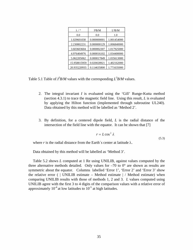
λ / ° I³B/M L³B/M

0.0 0.0 1.0 1.029601030 0.000000001 1.001454000 2.230802231 0.000000129 1.006840000 3.603603604 0.000002307 1.017925000 4.976404976 0.000016102 1.034400000 5.062205062 0.000017849 1.035613000

15.958815959 0.020028921 1.402162000 20.935220935 0.114635800 1.771635000

Table 5.1 Table of I3B/M values with the corresponding L3B/M values.

2. The integral invariant I is evaluated using the ‘Gill’ Runge-Kutta method (section 4.3.1) to trace the magnetic field line. Using this result, L is evaluated by applying the Hilton function (implemented through subroutine UL240). Data obtained by this method will be labelled as ‘Method 2’.

3. By definition, for a centered dipole field, L is the radial distance of the intersection of the field line with the equator. It can be shown that [7]

λ2cosLr =

(5.3) where r is the radial distance from the Earth´s center at latitude λ.

Data obtained by this method will be labelled as ‘Method 3’. Table 5.2 shows L computed at 1 Re using UNILIB, against values computed by the

three alternative methods detailed. Only values for –70 to 0° are shown as results are symmetric about the equator. Columns labelled ‘Error 1’, ‘Error 2’ and ‘Error 3’ show the relative error ( | UNILIB estimate – Method estimate | / Method estimate) when comparing UNILIB results with those of methods 1, 2 and 3. L values computed using UNILIB agree with the first 3 to 4 digits of the comparison values with a relative error of approximately 10-4 at low latitudes to 10-5 at high latitudes.

35

λ / ° L / Re Relative error

UNILIB Method 1 Method 2 Method 3 Error 1 Error 2 Error 3 -70 8.5491 8.5486 8.5493 8.5486 5.85E-05 2.34E-05 5.85E-05 -60 4.0002 4.0000 4.0004 4.0000 5.00E-05 5.00E-05 5.00E-05 -50 2.4202 2.4203 2.4204 2.4203 4.13E-05 8.26E-05 4.13E-05 -40 1.7038 1.7041 1.7040 1.7041 1.76E-04 1.17E-04 1.76E-04 -30 1.3330 1.3333 1.3332 1.3333 2.25E-04 1.50E-04 2.25E-04 -20 1.1322 1.1325 1.1324 1.1325 2.65E-04 1.77E-04 2.65E-04 -10 1.0309 1.0311 1.0311 1.0311 1.94E-04 1.94E-04 1.94E-04 0 1.0000 1.0000 1.0000 1.0000 0.0 0.0 0.0

Table 5.2 Comparison of values of L computed using UNILIB and three alternative methods, computed using the centered dipole model, at points located at different geographic latitudes, and at a radius of 1 Re.

Table 5.3 shows L computed at 3 Re. Again, the relative error varies from 10-4 to 10-5.

λ / ° L / Re Relative error

UNILIB Method 1 Method 2 Method 3 Error 1 Error 2 Error 3 -70 25.6472 25.6459 25.6479 25.6459 5.07E-05 2.73E-05 5.07E-05 -60 12.0004 12.0000 12.0012 12.0000 5.33E-05 6.67E-05 3.33E-05 -50 7.2604 7.2608 7.2612 7.2608 5.51E-04 1.10E-04 5.51E-05 -40 5.1113 5.1123 5.112 5.1123 1.96E-04 1.37E-04 1.96E-04 -30 3.9988 4.0000 3.9996 4.0000 3.00E-04 2.00E-04 3.00E-04 -20 3.3964 3.3974 3.3972 3.3974 2.94E-04 2.35E-04 2.94E-04 -10 3.0925 3.0933 3.0932 3.0933 2.59E-04 2.26E-04 2.59E-04 0 3.0000 3.0000 3.0000 3.0000 0.0 0.0 0.0

Table 5.3 Comparison of values of L computed using UNILIB and three alternative methods, computed using the centered dipole model, at points located at different geographic latitudes, and at a radius of 3 Re.

5.2. IGRF model For the IGRF model, L values computed by UNILIB were checked with values

computed using method 2 (methods 1 and 3 not being applicable). The integral invariant I is evaluated using the Runge-Kutta adaptive method (section 4.3.1) to trace the

36

magnetic field line (as detailed earlier, L is calculated by applying the Hilton function). Table 5.4 shows L computed using UNILIB and the RK adaptive program for the IGRF 1985 model at 1 and 3 Re and 0° longitude. The UNILIB and RK adaptive results agree to the first 3 or 4 digits. The relative error is typically 10-4 though occasionally 10-5 at high latitudes. (UNILIB data for 70° and 3 Re was unavailable as the field line was traced outside the magnetosphere and an error was returned.)

λ / ° 1 Re L / Re 3 Re L / Re

UNILIB RK adaptive Error UNILIB RK adaptive Error -70 4.168775 4.169125 8.40E-05 15.06390 15.0656 1.13E-04 -60 3.025265 3.02555 9.41E-05 9.104072 9.104985 1.00E-04 -50 2.391761 2.392082 1.34E-04 6.289990 6.291489 2.38E-04 -40 1.962656 1.963004 1.77E-04 4.789172 4.790518 2.81E-04 -30 1.63025 1.630488 1.48E-04 3.929591 3.930537 2.41E-04 -20 1.363903 1.364127 1.64E-04 3.430258 3.431355 3.20E-04 -10 1.162879 1.163185 2.63E-04 3.166793 3.167387 1.87E-04 0 1.035128 1.035269 1.37E-04 3.086154 3.086198 1.41E-05 10 0.984606 0.984623 1.76E-05 3.179744 3.180724 3.08E-04 20 1.017085 1.017244 1.56E-04 3.485356 3.486234 2.51E-04 30 1.161496 1.161737 2.07E-04 4.099315 4.100402 2.65E-04 40 1.499581 1.499838 1.72E-04 5.246298 5.247378 2.06E-04 50 2.222984 2.223192 9.36E-05 7.47172 7.472943 1.64E-04 60 3.633795 3.633871 2.10E-05 12.32155 12.322449 7.30E-05 70 7.481709 7.481518 2.55E-05 N/A 25.2488 N/A

Table 5.4 Comparison of L values computed using UNILIB and the Runge-Kutta adaptive method (the value of I is evaluated using RK adaptive to trace the field line, using the Hilton function L is calculated from this I value), computed using the IGRF model, at points located at different geographic latitudes, at a radius of 1 and 3 Re, along the meriodian 0° longitude, and epoch 1985.

5.2.1. Computation time

The computer evaluation time for evaluation of values of L using the IGRF model was, again, very rapid. On a Hewlett-Packard Workstation, 100 L values were evaluated in 1.15 seconds.

37

5.3. The Hilton function Subroutine UL240 (evaluate the Hilton function) can be simply checked by examining

the centered dipole model. UL230 (evaluate the integral invariant coordinate I ) is used to compute values of I. Using these values of I, values of I3B/M are calculated, which, using Table 5.1, allows values of L3B/M and therefore L to be calculated. L computed using this method will be labelled as ‘method 1’ and will be compared to L obtained by subroutine UL220 (get information on magnetic field line), labelled as ‘method 2’.

Table 5.5 shows values of L returned using the two methods at points located at

different geographic latitudes and at a radius of 3 Re. The relative error ranges from 10-4 at high latitudes to 10-5 at low latitudes indicating that the Hilton function is accurately implemented through subroutine UL240.

λ / ° L / Re Error

Method 1 Method 2 -70 8.546602 8.549134 3.00E-04 -60 3.999339 4.000219 2.20E-04 -50 2.419937 2.420231 1.21E-04 -40 1.703843 1.703837 4.18E-04 -30 1.333123 1.333018 7.81E-05 -20 1.132286 1.132223 5.63E-05 -10 1.030916 1.030913 3.72E-04 0 1.000000 1.000000 0.0 10 1.030919 1.030916 3.69E-04 20 1.132288 1.132225 5.63E-05 30 1.333123 1.333019 7.81E-05 40 1.703844 1.703837 4.17E-04 50 2.419938 2.420231 1.21E-04 60 3.999339 4.000219 2.20E-04 70 8.546603 8.549134 2.96E-04

Table 5.5 Verification of subroutine UL240 (evaluate the Hilton function). Comparison of L values computed using UNILIB (Method 2) and an alternative method (Method 1), computed using the centered dipole model, at points located at different geographic latitudes, and at a radius of 3 Re.

38

5.3.1. The inverse Hilton function The reverse transformation, subroutine UL242 (inverse the Hilton function),

determines the integral invariant I from the magnetic shell parameter L. Column 2 of Table 5.6 shows I (labelled Iinitial) for the IGRF 1995 model at 2 Re and 320° longitude. These I values are transformed to L by UL240 (evaluate the Hilton function) and then transformed back to I (shown in column 3 as Ifinal) by subroutine UL242. The I values of columns 2 and 3 are in good agreement, as expected, validating subroutine UL242. [The relative error is an order of magnitude smaller at low latitudes than high latitudes This is possibly due to the inaccuracy in the calculation of L (see Table 5.4), which is slightly greater at high latitudes and which may be amplified during the reverse transformation.]

λ / ° Iinitial Ifinal Error 0 754.90712 754.90711 2.00E-08 10 3910.1963 3910.1944 4.92E-07 20 10039.269 10039.242 2.65E-06 30 20814.281 20814.115 7.97E-06 40 40484.986 40484.290 1.72E-05 50 80601.792 80599.408 2.96E-05 60 180342.185 180334.482 4.27E-05 70 539626.740 539597.902 5.34E-05 80 2839629.087 2839461.843 5.89E-05

Table 5.6 Verification of subroutine UL242 (inverse the Hilton function). Comparison of I values (Iinitial) which are transformed first to L values using subroutine UL240 and then back to I using subroutine UL242 (Ifinal). Computed using the IGRF model, at points located at different geographic latitudes, at a radius of 2 Re, along the meriodian 320° longitude, and epoch 1995.

5.4. Evaluation of arc length Besides evaluating L, subroutine UL220 (get information on a magnetic field line

segment) computes the arc length of a magnetic field line between mirror points.

39

5.4.1. Centered dipole model For a centered dipole field, the length of the magnetic field line can be written as [7]

λλλ

λ

dLl ∫ +=max

0

²sin31cosRe (5.4)

This integral was evaluated using the integration routine DGAUSS [10]. Table 5.7

shows l computed at 3 Re using UNILIB subroutine UL220 and by integrating (5.4). Comparing the two sets of data, the relative error varies from 10-5 to 10-7 indicating the arc length l is reliably evaluated by UNILIB. Note that UNILIB results are more accurate at high rather than low latitudes.

λ / ° l / km Error UNILIB Exact

-70 412498.26 412498.95 1.68E-06 -60 172102.5 172101.9 3.54E-06 -50 88115.77 88114.95 9.32E-06 -40 49370.97 49370.15 1.67E-05 -30 28383.3 28382.6 2.59E-05 -20 15631.9 15631.3 3.59E-05 -10 6946.3 6945.8 7.64E-05 0 0.0 0.0 0.0 10 6946.33 6946.29 6.05E-06 20 15631.86 15631.81 2.88E-06 30 28383.34 28383.28 1.94E-06 40 49370.97 49370.92 1.13E-06 50 88115.77 88115.68 9.87E-06 60 172102.51 172102.38 7.32E-07 70 412498.26 412498.13 3.25E-07

Table 5.4 Comparison of UNILIB and ‘exact’ values of the magnetic field line length l, computed using the centered dipole model, at points located at different geographic latitudes, and at a radius 3 Re

40

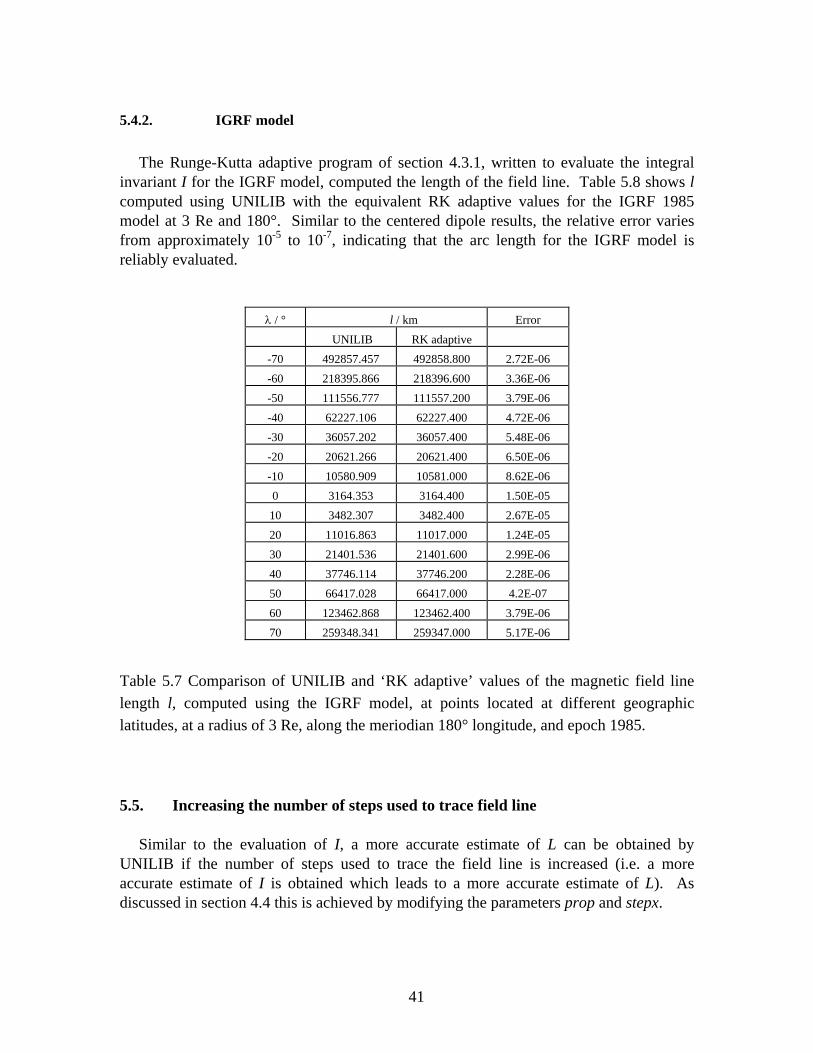
5.4.2. IGRF model The Runge-Kutta adaptive program of section 4.3.1, written to evaluate the integral

invariant I for the IGRF model, computed the length of the field line. Table 5.8 shows l computed using UNILIB with the equivalent RK adaptive values for the IGRF 1985 model at 3 Re and 180°. Similar to the centered dipole results, the relative error varies from approximately 10-5 to 10-7, indicating that the arc length for the IGRF model is reliably evaluated.

λ / ° l / km Error

UNILIB RK adaptive -70 492857.457 492858.800 2.72E-06 -60 218395.866 218396.600 3.36E-06 -50 111556.777 111557.200 3.79E-06 -40 62227.106 62227.400 4.72E-06 -30 36057.202 36057.400 5.48E-06 -20 20621.266 20621.400 6.50E-06 -10 10580.909 10581.000 8.62E-06 0 3164.353 3164.400 1.50E-05 10 3482.307 3482.400 2.67E-05 20 11016.863 11017.000 1.24E-05 30 21401.536 21401.600 2.99E-06 40 37746.114 37746.200 2.28E-06 50 66417.028 66417.000 4.2E-07 60 123462.868 123462.400 3.79E-06 70 259348.341 259347.000 5.17E-06

Table 5.7 Comparison of UNILIB and ‘RK adaptive’ values of the magnetic field line length l, computed using the IGRF model, at points located at different geographic latitudes, at a radius of 3 Re, along the meriodian 180° longitude, and epoch 1985.

5.5. Increasing the number of steps used to trace field line Similar to the evaluation of I, a more accurate estimate of L can be obtained by

UNILIB if the number of steps used to trace the field line is increased (i.e. a more accurate estimate of I is obtained which leads to a more accurate estimate of L). As discussed in section 4.4 this is achieved by modifying the parameters prop and stepx.

41

5.5.1. IGRF model Table 5.9 is similar to 5.4, but with L computed using modified values of prop= 0.02,

stepx= 0.02, kum533 < 0 and xbmin= 1.0E-07 Gauss. The relative error of the UNILIB data varies from 10-5 at low latitudes to 10-7 at high latitudes, two orders of magnitude less than the relative errors of Table 5.4 (calculated using the default parameter values). As discussed, reducing the value of prop from 0.2 to 0.02 increases the number of steps used to trace the field line by a factor of 10.

λ / ° 1 Re L / Re 3 Re L / Re UNILIB RK adaptive Error UNILIB RK adaptive Error

-70 4.168943 4.169038 2.28E-05 15.065327 15.065418 6.05E-06 -60 3.025448 3.025489 1.35E-05 9.104873 9.104912 4.27E-06 -50 2.392016 2.392030 5.94E-06 6.291418 6.291436 2.86E-06 -40 1.962969 1.962972 1.38E-06 4.79047 4.79048 5.09E-07 -30 1.630461 1.630463 1.41E-06 3.930506 3.930508 5.07E-07 -20 1.364104 1.364101 1.83E-06 3.431336 3.431337 2.91E-07 -10 1.163167 1.163166 7.74E-07 3.167378 3.167378 0.0 0 1.035258 1.035258 2.90E-07 3.0861973 3.086197 9.72E-08 10 0.984621 0.984621 3.05E-07 3.1807125 3.180712 1.57E-07 20 1.017227 1.017227 9.83E-08 3.4862166 3.486215 4.59E-07 30 1.161708 1.161706 1.64E-06 4.100385 4.10038 1.22E-06 40 1.499810 1.499802 5.20E-06 5.2473766 5.247363 2.59E-06 50 2.223196 2.223177 8.32E-06 7.4729844 7.472954 4.36E-06 60 3.633973 3.633917 1.54E-05 12.3226 12.32253 5.68E-06 70 7.481921 7.481764 2.10E-05 25.249267 25.249092 6.93E-06

Table 5.8 Comparison of L values computed using UNILIB and the Runge-Kutta adaptive method (the value of I is evaluated using RK adaptive to trace the field line, using the Hilton function L is calculated from this I value), computed using the IGRF model, at points located at different geographic latitudes, at a radius of 1 and 3 Re, along the meriodian 0° longitude, and epoch 1985. Results are computed using the modified values of prop= 0.02, stepx= 0.02, kum533 < 0 and xbmin= 1.0E-07 Gauss.

42

5.5.2. Computation time

Using the modified values of prop= 0.02 and stepx= 0.02 the computer evaluation time was, surprisingly, unchanged. Using a Hewlett-Packard Workstation it still took approximately 1.15 seconds to evaluate 100 L values using UNILIB subroutines.

5.6. Recommendations For the IGRF model, L computed using UNILIB subroutine UL220 had a relative

error of between 10-4 to 10-5. It was shown that by increasing the number of steps used to trace the field line by a factor of 10 the relative error was reduced to 10-5 to 10-7. It is recommended that a parameter is introduced in subroutine UL220 allowing the user to choose the desired accuracy of L.

43

6. Evaluation of the lowest altitude of mirror points

6.1. Introduction The drift shell is defined as a set of magnetic field line segments characterized by the

same integral invariant I, shell parameter L and magnetic field intensity Bm at the mirror point. Typically, the altitude of the mirror points will vary with latitude and longitude. An important geomagnetic quantity is to determine the geographic positions of the mirror points of lowest altitude in the northern and southern hemisphere and the lowest altitude hmin. Within UNILIB, this is achieved by either subroutine UD315 (search the mirror point of lowest altitude) or subroutine UD317 (trace a magnetic drift shell [new]). Rather than examine the location of the lowest altitude mirror point, this section will examine UNILIB’s evaluation of the minimum altitude hmin.

Subroutine UD315 scans the field line segments of a drift shell and determines the geographic positions of the mirror points with the lowest altitude in the northern and southern hemisphere [also required is subroutine UD310 (trace a magnetic drift shell)]. (In the UNILIB library, see Example 4 (page 88) for a sample program to search the point with lowest altitude on a magnetic drift shell.)

Subroutine UD317 traces a magnetic drift shell (used as an alternative to UD310) and

returns the altitude of the lowest mirror point (though not its geographic position).

6.2. Centered dipole model For a centered and aligned dipole model, the altitude hmin of the lowest mirror point is

defined as [7]

λ²cosReReminmin Lah =+= (6.1)

where amin is the minimum altitude above the Earth surface (Re, L and λ as previously

defined). Examining (6.1), the altitude of the lowest mirror point is independent of longitude.

As subroutine UD315 searches for the lowest mirror point position, as a function of longitude, by searching for an absolute minimum, it is not suitable for application to the centered dipole model. Therefore, for this instance, UD317 was applied to evaluate hmin.

Fig 6.1 shows the difference between UNILIB’s estimate of hmin and the ‘exact’ value

computed using (6.1) for combinations of B and L. The drift shell parameter L varies between 1 and 5 and the magnetic field of the mirror points varies between 0.01 and 0.35

44

Gauss. The relative difference between the two estimates is strongly dependent on the magnetic field strength B with points at high B (close to the Earth) having a relative difference less than 0.25 km and as B decreases (distance increasing from the Earth) the relative difference increasing to a maximum of around 2 km.

0.01

0.07

0.13

0.19

0.25

0.31

1.00

1.56

2.13

2.69

3.26

3.82

-0.5

0

0.5

1

1.5

2

2.5

Diff

eren

ce (k

m)

B intensity (Gauss)L parameter (Re)

Figure 6.1 Relative difference between UNILIB and exact estimate of hmin, computed using the centered dipole model for different combinations of B and L.

6.3. IGRF model As the exact formula (6.1) is not applicable for the IGRF model, section (6.3.1) describes an

alternative method of computing hmin.

6.3.1. Alternative method of evaluating hmin As discussed, a drift shell is characterized by a ring of mirror points BBm and a surface of

constant L. Figure 6.2 shows a line of constant B (B = BconstantB ) and a line of constant L (L= Lconstant) around the Earth. The ring of mirror points will lie on the intercept of the B

45

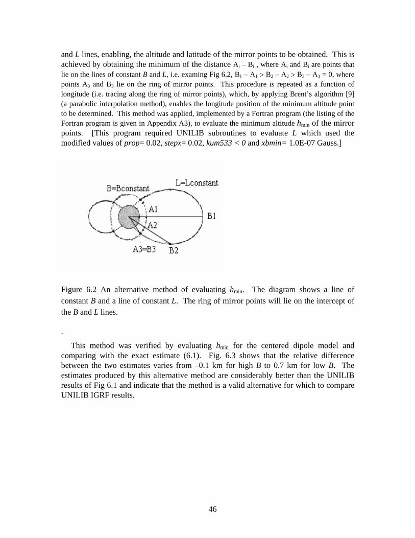
and L lines, enabling, the altitude and latitude of the mirror points to be obtained. This is achieved by obtaining the minimum of the distance Ai – Bi , where Ai and Bi are points that lie on the lines of constant B and L, i.e. examing Fig 6.2, B1 – A1 > B2 – A2 > B3 – A3 = 0, where points A3 and B3 lie on the ring of mirror points. This procedure is repeated as a function of longitude (i.e. tracing along the ring of mirror points), which, by applying Brent’s algorithm [9] (a parabolic interpolation method), enables the longitude position of the minimum altitude point to be determined. This method was applied, implemented by a Fortran program (the listing of the Fortran program is given in Appendix A3), to evaluate the minimum altitude hmin of the mirror points. [This program required UNILIB subroutines to evaluate L which used the modified values of prop= 0.02, stepx= 0.02, kum533 < 0 and xbmin= 1.0E-07 Gauss.]

Figure 6.2 An alternative method of evaluating hmin. The diagram shows a line of constant B and a line of constant L. The ring of mirror points will lie on the intercept of the B and L lines.

.

This method was verified by evaluating hmin for the centered dipole model and comparing with the exact estimate (6.1). Fig. 6.3 shows that the relative difference between the two estimates varies from –0.1 km for high B to 0.7 km for low B. The estimates produced by this alternative method are considerably better than the UNILIB results of Fig 6.1 and indicate that the method is a valid alternative for which to compare UNILIB IGRF results.

46

0.01

0.06

0.11

0.16

0.21

0.26

0.31

1.00

1.47

1.94

2.41

2.88

3.35

3.82

-0.1

0

0.1

0.2

0.3

0.4

0.5

0.6

0.7

Diff

eren

ce (k

m)

B intensity (Gauss)L parameter (Re)

Figure 6.3 Verification of the alternative method of calculating hmin. Relative difference between the alternative and exact estimate of hmin, computed using the centered dipole model for different combinations of B and L.

6.3.2. Results Fig 6.4 shows the difference between UNILIB’s estimate of hmin (computed using

subroutine UD315) and the estimate computed using the alternative method for combinations of B and L and epoch 1985. The difference between the two estimates is typically less than 0.5 km, though, for low B (far from the Earth surface) the difference increases to a maximum of around 2.5 km.

47

0.01

0.03

0.06

0.09

0.12

0.15

0.18

1.50

1.96

2.42

2.88

3.34

3.79

-0.5

0

0.5

1

1.5

2

2.5

Diff

eren

ce (k

m)

B intensity (Gauss)L parameter (Re)

Figure 6.4 Relative difference between UNILIB and alternative estimate of hmin, computed using the IGRF model for different combinations of B and L and epoch 1985.

6.3.3. Computation time Using a Hewlett-Packard Workstation it took approximately 1 second for UNILIB to

evaluate hmin for each combination of B and L.

6.4. Increasing the number of steps used to trace field line As discussed in section 5.5, the accuracy that UNILIB computes L can be increased if

the parameters prop and stepx are modified from their default values. This section examines UNILIB estimates of hmin computed using the modified values prop= 0.02 and stepx= 0.02.

6.4.1. Centered dipole model Fig. 6.5 is similar to Fig. 6.1 but with UNILIB using the modified values. The

UNILIB results are substantially more accurate with the maximum difference between the two sets of results now 0.4 km, while for points close to the Earth’s surface (high B,

48

low L) the relative difference is almost zero.

0.01

0.07

0.13

0.19

0.25

0.31

1.00

1.47

1.94

2.41

2.88

3.35

3.82

-0.20

-0.10

0.00

0.10

0.20

0.30

0.40

0.50D

iffer

ence

s (km

)

B intensity (Gauss)L parameter (Re)

Figure 6.5 Relative difference between UNILIB and exact estimate of hmin, computed using the centered dipole model for different combinations of B and L. Results are computed using the modified values of prop= 0.02 and stepx= 0.02.

6.4.2. IGRF model Fig. 6.6 is similar to Fig. 6.4 but with UNILIB using the modified values. Again,

UNILIB results are substantially more accurate with the maximum difference now 0.3 km, while for points close to the Earth’s surface the relative difference is approximately 0.15 km.

49

0.01

0.07

0.13

0.20

1.50

1.73

1.96

2.192.42

2.65

2.88

3.11

3.343.56

3.79

4.10

-0.35

-0.30

-0.25

-0.20

-0.15

-0.10

-0.05

0.00

0.05

0.10

0.15

0.20

diffe

renc

e (k

m)

B intensity (Gauss)

L parameter (Re)

Figure 6.6 Relative difference between UNILIB and alternative estimate of hmin, computed using the IGRF model for different combinations of B and L and epoch 1985. Results are computed using the modified values of prop= 0.02 and stepx= 0.02.

6.5. Recommendations Increasing the number of steps used to trace the field lines significantly improved the

accuracy that UNILIB computes hmin. Similar to chapters 4 and 5, it is recommended that a input parameter is introduced that allows the user to choose the desired accuracy that hmin is computed.

.

50

7. Conclusion

This report has confirmed the usefulness of the UNILIB Fortran library (version 2.03) in calculating some of the basic geomagnetic quantities, such as, the (B, L) coordinates, the third adiabatic invariant I and the altitude of the lowest mirror point hmin (the accurate evaluation of these quantities indicates UNILIB’s ability to trace magnetic field lines and drift shells). The validation was for the centered dipole model, IGRF model, and, for the external magnetic field, Tsyganenko’s model. The centered dipole model, though not particularly realistic, was useful as ‘exact’ analytical expressions were often available. Given below is a summary of UNILIB´s implementation of the IGRF model in the calculation of B, I, L and hmin. UNILIB was applied to evaluate the geomagnetic field strength, with results in excellent agreement with the ‘benchmark’ GEOPACK and exact analytical results.

UNILIB’s estimation of I, for the IGRF model, showed a relative error of between 10-3

and 10-4, though, by increasing by a factor of 10 the number of steps used to trace the field line (modified values of prop= 0.02 and stepx= 0.02 in common block UC190), the relative error decreased to between 10-4 and 10-5 (though at the expense of a longer computation time). It is shown in chapter 4 how to modify the parameters prop and stepx, though it is recommended that UNILIB be adapted so that, rather than altering the value of prop, a parameter is introduced allowing control over the number of steps used to trace a field line or the accuracy of I returned.

UNILIB’s estimation of L, for the IGRF model, showed a relative error of between

10-4 and 10-5. Again, by increasing the number of steps to trace the field line by a factor of 10, the relative error decreased to between 10-6 and 10-7. It was again recommended that some control over the accuracy of L returned be introduced.

UNILIB’s estimation of the minimum altitude of a drift shell hmin, for the IGRF

model, was accurate to within 0.3 to 3 km (the disagreement increasing as the distance from the Earth increased). Increasing the number of steps used to trace a field line by a factor of 10 reduced the disagreement to between 0.15 and 0.3 km for all combinations of B and L examined. Again, it is recommended that a parameter be introduced allowing control over the accuracy of hmin returned. It was shown that the accuracy of I, L and hmin could be substantially improved if the number of steps used to trace field lines was increased. It was recommended that, within the Fortran subroutines, an input parameter is introduced that allows the user to either select the accuracy with which a field line is traced or the accuracy of the particular geomagnetic parameter returned. This could be easily implemented in a future version of UNILIB.

51

This study has shown that the UNILIB software library is an accurate and reliable method of computing basic geomagnetic quantities. In general it was found that the library was easy to use and of great use to the magnetospheric modelling community.

52

References

[1] http://www.magnet.oma.be/home/unilib [2] www-spof.gsfc.nasa.gov/Modeling/geopack.html [3] http://nssdc.gsfc.nasa.gov/space/model/magnetos/bilcal.html [4] Russell, R. T., ‘Geophysical Coordinate Transformations’, Cosmic Electrodynamics, Vol. 2, pp. 184-196, 1971. [5] ‘Handbook of geophysics and the space environment’, Air Force Geophysics Laboratory, Hancolm, MA., Rept. No. ADA 167 000, avail. from NTIS (Nat. Tech. Inf. Service, U.S. Dept. of Commerce, Springfield, Va., 22161), chapter 4, 1985. [6] Tsyganenko, N. A., ‘A magnetospheric magnetic field model with a warped tail current sheet’, Planet. Space Sci., Vol. 37, No. 1, pp 5-20, 1989. [7] Hess, W. N., The Radiation Belt and Magnetosphere, Blaisdell Publishing Company, Waltham MA., 1968. [8] McIlwain, C. E., ‘Coordinates for mapping the distribution of magnetically trapped particles’, Journal of Geophysical Research, Vol. 66, No. 11, pp 3681-3691, Nov 1961. [9] http://www.ulib.org/webRoot/Books/Numerical_Recipes [10] http://wwwinfo.cern.ch/asd/cernlib/libraries.html

53

Appendix A.1 Fortran program to compute I for centered dipole model *****************************************************$ ***This program compute the integral invariant belongs ***to the McIlwain's article "coordinates for mapping ***the distribution of magnetically trapped particles ***Journal of Geophysical research Vol 66 No 11 1961 program EVABL

implicit double precision (a-z) real value,tier real*8 i,pi,r0 REAL*8 gcolat,gradius,glong,i3bm,bpos,moment COMMON/GEOPOS/gcolat,gradius,glong COMMON/RESULT/I3BM,BPOS,MOMENT common/INVA/invari call initnorvar ***moment is year dependent the value below is for the 1995 year** moment=0.30207661 do i=90.,10.,-10. pi=4.d0*atan(1.) **** define geographic position******** glong=0. gradius=6371.2 gcolat=i la=(gcolat)*pi/180.d0 ***compute the equatorial radial distance r0=gradius/dcos(la)**2. ***** print the latitude and the I belongs to the article formula print*,90.-gcolat,100000*(funh1(la)*moment*(gradius/r0)**3.) enddo stop end ***** compute the invariant I at a latitude lamda, see equation 1of article *** real*8 function funh1(lat) implicit double precision (a-z) common/LATIT/latmir external integrand zero = 0. eps = 0.001 latmir=dabs(lat) sinlatmir = dsin(latmir) funh1 = dgauss(integrand,zero,sinlatmir,eps) return end

54

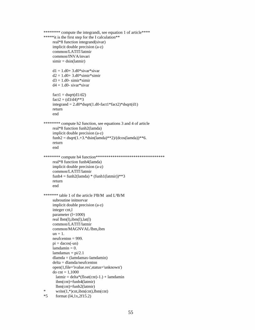
******** compute the integrandi, see equation 1 of article**** *****it is the first step for the I calculation** real*8 function integrand(sivar) implicit double precision (a-z) common/LATIT/latmir common/INVA/invari simir = dsin(latmir) d1 = 1.d0+ 3.d0*sivar*sivar d2 = 1.d0+ 3.d0*simir*simir d3 = 1.d0- simir*simir d4 = 1.d0- sivar*sivar fact1 = dsqrt(d1/d2) fact2 = (d3/d4)**3 integrand = 2.d0*dsqrt(1.d0-fact1*fact2)*dsqrt(d1) return end ******** compute h2 function, see equations 3 and 4 of article real*8 function funh2(lamda) implicit double precision (a-z) funh2 = dsqrt(1.+3.*dsin(lamda)**2)/(dcos(lamda))**6. return end ******** compute h4 function********************************* real*8 function funh4(lamda) implicit double precision (a-z) common/LATIT/latmir funh4 = funh2(lamda) * (funh1(latmir))**3 return end ******* table 1 of the article I³B/M and L³B/M subroutine initnorvar implicit double precision (a-z) integer cnt,l parameter (l=1000) real lbm(l),ibm(l),lat(l) common/LATIT/latmir common/MAGNVAL/lbm,ibm un = 1. neufcentnn = 999. pi = dacos(-un) lamdamin = 0. lamdamax = pi/2.1 dlamda = (lamdamax-lamdamin) delta = dlamda/neufcentnn open(1,file='ivalue.res',status='unknown') do cnt = 1,1000 latmir = delta*(float(cnt)-1.) + lamdamin ibm(cnt)=funh4(latmir) lbm(cnt)=funh2(latmir) * write(1,*)cnt,ibm(cnt),lbm(cnt) *5 format (I4,1x,2f15.2)

55

enddo close(1) return end *******interpolation **************** ****used for interpolation in the previously computed table real*8 function interpol(val) implicit double precision (a-z) integer l parameter (l=1000) real lbm(l),ibm(l) real val common/MAGNVAL/lbm,ibm interpol=divdif(lbm,ibm,l,val,1) return end

56

A.2 Fortran program to compute I for IGRF model program main implicit double precision (a-z) double precision totlong,xf integer ifail INCLUDE 'structure.h' COMMON/FIELD/bmod,brho,btheta,bphi COMMON/GLOB/eps,re1 COMMON/END1/totlong COMMON/END2/xf COMMON/PAS/dlf COMMON/LMA/lva RECORD/ZGEO/mpos RECORD/ZVEC/mb,mnr do a=60.d0,80.d0,10. call initialise alt=re1 ala=a alo=0.d0 alt=3.*re1 dlf=0.7 test=lvalue(alt,alo,ala) write(6,111)test,lva,totlong,ala 111 format(4(1x,f18.6)) enddo stop end ************************************************$ double precision function lvalue(alt,alo,ala) double precision alt,alo,ala,bmod,brho,btheta,bphi,bmir,integr real*8 pi,deg,re,gmagmo,eclipt, geoid(3),uma(30) real*8 xrmin,xbmin,xtmin,xbmax,epslon,epsfl real*8 prop,stepx,stpmin,umsq,upsq,uk2,uk3 double precision invaria,eps,re1 real*8 fvet,pvet,epsomeg,dltalt real*8 epskm,epsrel real*8 stplst,xclat real*8 lva integer flag,modf,okstep,dir integer*4 kmflg,kum533 integer i,dim,a INCLUDE 'structure.h' COMMON/FIELD/bmod,brho,btheta,bphi COMMON/STOP/flag,modf,okstep,dir COMMON/MIRR/bmir,integr COMMON/GLOB/eps,re1 COMMON/INVA/invaria RECORD/ZLBL/mlab

57

RECORD/zfln/mlin RECORD/zseg/mele(nx170) RECORD/ZIMF/mint RECORD/Zsun/msun RECORD/Zemf/mext COMMON/UC192/xrmin,xbmin,xtmin,xbmax,epslon,epsfl,fvet,pvet, * epsomeg,dltalt COMMON/UC190/prop,stepx,stpmin,umsq,upsq,uk2,uk3,epskm,epsrel, * stplst,xclat,kmflg,kum533 COMMON /UC170/nsg,kgp,mlab,mlin,mele COMMON /UC160/ pi,deg,re,gmagmo,eclipt,geoid,uma COMMON/UC140/ mint,mext,msum COMMON/LMA/lva * compute magnetic field vector call afield (alt,alo,ala) bmir=bmod * follow magnetic field line towards the north call tracenorth(alt,alo,ala) call revers if(flag.eq.1)then flag =0 modf=0 okstep=0 * follow magnetic field line towards the south

call tracesouth(alt,alo,ala) endif * compute invariant I call invarian mlab.finv=invaria mlab.fbmp=bmir mlab.linv=.TRUE. mlab.lbmp=.TRUE. * for dipolar field remmove comment * gmagmo=mint.gmmo * Use Hilton function to compute L from I call UL240(mlab,ifail) if(ifail.lt.0)then print*,ifail endif

58

* lva is the integral invariant I value and lvalue is the McIlwain parameter L lva=invaria lvalue=mlab.flmi return end *****************************************************************$$ subroutine initialise INCLUDE 'structure.h' INTEGER*4 kunit, kinit, ifail, kint, kext, nfbm, noprint CHARACTER*32 lbint, lbext REAL*8 year, param(10) real*8 pi,deg,re,gmagmo,eclipt, geoid(3),uma(30) real*8 xrmin,xbmin,xtmin,xbmax,epslon,epsfl real*8 prop,stepx,stpmin,umsq,upsq,uk2,uk3 real*8 fvet,pvet,epsomeg,dltalt double precision eps,re1,bmir,dlf real*8 epskm,epsrel real*8 stplst,xclat integer*4 kmflg,kum533 integer flag,modf,okstep,dir COMMON/UC192/xrmin,xbmin,xtmin,xbmax,epslon,epsfl,fvet,pvet, * epsomeg,dltalt COMMON/UC190/prop,stepx,stpmin,umsq,upsq,uk2,uk3,epskm,epsrel, * stplst,xclat,kmflg,kum533 COMMON/UC160/ pi,deg,re,gmagmo,eclipt,geoid,uma COMMON/UC140/ mint,mext,msum COMMON/STOP/flag,modf,okstep,dir COMMON/MIRR/bmir,integr COMMON/INTER/var,inte COMMON/GLOB/eps,re1 RECORD /zimf/ mint RECORD /zsun/ msun RECORD /zemf/ mext RECORD/ZDAT/ mdate C C initialisation C DATA kunit, kinit, kint, kext, nfbm, noprint/ 0, 1, 0, 0, 1, -1/ DATA year, param/ 1985.0d0, 10*0.0d0/ eps=0.00001 re1=6371.2 flag =0 modf=0 okstep=0 dir=1 mdate.iyear = 1985 mdate.imonth = 1 mdate.iday = 1 mdate.ihour = 0

59

mdate.imin = 0 mdate.secs = 0.0d0 C *Initialize the UNILIB library CALL UT990 (kunit, kinit, ifail) IF( ifail .LT. 0 )STOP * modify some values to trace magnetic field line outside the magnetopause xbmin=0.00000001 xrmin=0.1 kum533=-1 xbmax=100000000. * set geomagnetic field model CALL UM510 (kint, year, lbint, kunit, ifail) IF( ifail .LT. 0 )STOP * for centered dipol field remove comments * mint.norder = 2 * mint.label = 'Dipolar magnetic field ' * mint.coef(2,1) = mint.gmmo * 1.0d+05 * mint.coef(1,2) = 0.0d+00 * mint.coef(2,2) = 0.0d+00 * mint.elong = 0.0d+00 * mint.colat = 0.0d+00 CALL UT540 (mdate) CALL UM520 (kext, mdate.amjd, param,lbext, kunit, ifail) IF( ifail .LT. 0 )STOP return end ******************************************************* subroutine tracenorth(alt,alo,ala) * this subroutine trace a magnetic field line in the northem direction

* and store the length of the field line already computed as well as the integrand mB

B−1

double precision bopti,altopti,latopti,lonopti,newdlopt,integropti double precision aintegr(3100000),atrajet(3100000),b(3100000) double precision var(3100000),inte(3100000) double precision newalt,newlat,newlon,newdl double precision alt,ala,alo double precision bmir,integr double precision totlong double precision dlf integer flag,modf,okstep,dir integer i,dim

60

COMMON/OPT/bopti,altopti,latopti,lonopti,newdlopt,integropti COMMON/NEWP/newalt,newlat,newlon,newdl COMMON/END/totlong,aintegr,atrajet,b COMMON/STOP/flag,modf,okstep,dir COMMON/INTER/var,inte COMMON/MIRR/bmir,integr COMMON/NPAS/i,dim COMMON/PAS/dlf newdl=0. integr=0. * perform the first step towards the north call step (alt,alo,ala,dlf) call integrand aintegr(1)=integr atrajet(1)=newdl i=1

do while(flag.eq.0)

i=i+1 * perform one step towards the north call step(newalt,newlon,newlat,dlf)

* compute the integrand mB

B−1

call integrand if(modf.eq.0)then aintegr(i)=integr atrajet(i)=newdl else i=i inte(i)=integr var(i)=newdl endif enddo totlong=newdl return end *************************************************************** subroutine revers double precision aintegr(3100000),atrajet(3100000),b(3100000) double precision var(3100000),inte(3100000) double precision totlong integer i,n,dim,m COMMON/END/totlong,aintegr,atrajet,b COMMON/INTER/var,inte COMMON/NPAS/i,dim

61

* reverse the order in the table computed by trace north do n=i-1,0,-1 var(i-n)=dabs(atrajet(n+1)-totlong) inte(i-n)=aintegr(n+1) enddo dim=i-n-1 return end ******************************************************** subroutine tracesouth(alt,alo,ala) * trace magnetic field line towards the south double precision bopti,altopti,latopti,lonopti,newdlopt,integropti

double precision newalt,newlat,newlon,newdl double precision var(3100000),inte(3100000) double precision alt,ala,alo double precision bmir,integr double precision dlf integer flag,modf,okstep,dir integer m,i,dim COMMON/OPT/bopti,altopti,latopti,lonopti,newdlopt,integropti

COMMON/NEWP/newalt,newlat,newlon,newdl COMMON/STOP/flag,modf,okstep,dir COMMON/MIRR/bmir,integr COMMON/INTER/var,inte COMMON/END1/totlong double precision totlong COMMON/NPAS/i,dim COMMON/PAS/dlf dir=-1 m=i newdl=0. integr=0. call step (alt,alo,ala,dlf) call integrand do while(flag.eq.0) m=m+1 call step(newalt,newlon,newlat,dlf) call integrand if(modf.eq.0)then var(m+1)=newdl inte(m+1)=integr else m=m-1 var(m+1)=newdl inte(m+1)=integr endif dim=m+1 end do totlong=newdl return

62

end **************************************************** subroutine integrand

* compute the integrand mB

B−1

double precision integr,bmir double precision bmod,brho,btheta,bphi double precision oldalt,oldala,oldalo,oldbmod,dlold COMMON/MIRR/bmir,integr COMMON/FIELD/bmod,brho,btheta,bphi COMMON/OLD/oldalt,oldala,oldalo,oldbmod,dlold if(bmod.gt.bmir)then if((dabs(oldbmod-bmir)).le.1.0E-008)then integr=0. else integr=dsqrt(1.-(oldbmod/bmir)) endif else integr=dsqrt(1.-(bmod/bmir)) endif return end *********************************************************** subroutine afield (alt,alo,ala) * compute magnetis field INCLUDE 'structure.h' double precision alt,alo,ala double precision bmod,brho,btheta,bphi real*8 pi,deg,re,gmagmo,eclipt,geoid,uma real*8 xrmin,xbmin,xtmin,xbmax,epslon,epsfl real*8 fvet,pvet,epsomeg,dltalt real*8 prop,stepx,stpmin,umsq,upsq,uk2,uk3 real*8 epskm,epsrel real*8 stplst,xclat integer*4 kmflg,kum533 integer*4 ifail integer i,dim RECORD/Zvec/ mb RECORD/ZGEO/ mpos RECORD /zimf/ mint RECORD /zsun/ msun RECORD /zemf/ mext COMMON/NPAS/i,dim COMMON/UC140/ mint,mext,msum COMMON/FIELD/bmod,brho,btheta,bphi COMMON/UC160/pi,deg,re,gmagmo,eclipt,geoid,uma COMMON/UC190/prop,stepx,stpmin,umsq,upsq,uk2,uk3,epskm,epsrel, * stplst,xclat,kmflg,kum533

63

COMMON/UC192/xrmin,xbmin,xtmin,xbmax,epslon,epsfl,fvet,pvet, * epsomeg,dltalt ***set geographic position mpos.radius=alt mpos.colat=90.-ala mpos.elong=alo * compute geomagnetic field vector CALL UM530(mpos,mb,ifail) IF( ifail .LT. 0 )then print*,ifail,ala,mpos.colat stop endif bmod=mb.dnrm brho=mb.rho btheta=mb.theta bphi=mb.phi return end ********************************************************************* ***this subroutine set the step along the field line***** subroutine step (alt,alo,ala,dlf) * compute one step along the magnetic field line belongs to the Runge-Kutta adaptive method INCLUDE 'structure.h' double precision brho,btheta,bphi,bmod,alt,ala,alo,dlf double precision oldalt,oldala,oldalo,oldbmod,dlold double precision newalt,newlat,newlon,newdl double precision oldbphi, oldbthet, oldbrho real*8 pi,deg,re,gmagmo,eclipt,geoid,uma double precision bmir,integr double precision y(3),dydx(3),x,h,yout(3),you(3),yscale(3) real*8 htry,epss,hdid,hnext,xx integer flag,modf,okstep,dir,n COMMON/GLOB/eps,re1 COMMON/MIRR/bmir,integr COMMON/STOP/flag,modf,okstep,dir COMMON/FIELD/bmod,brho,btheta,bphi COMMON/NEWP/newalt,newlat,newlon,newdl COMMON/BOLD/oldbphi, oldbthet, oldbrho COMMON/OLD/oldalt,oldala,oldalo,oldbmod,dlold COMMON /UC160/ pi,deg,re,gmagmo,eclipt,geoid,uma COMMON/OUT/you COMMON/OUT1/xx RECORD/ZGEO/mpos,mpos1 call afield(alt,alo,ala) oldalt=alt oldala=ala oldalo=alo oldbmod=bmod oldbrho=brho

64

oldbthet=btheta oldbphi=bphi dlold=newdl mpos.radius=alt mpos.colat=90.-ala mpos.elong=alo y(1)=alt y(2)=90.-ala y(3)=alo ****vecteur deplacement**** sinthe=dsin(mpos.colat*deg) dydx(1)=brho/bmod dydx(2)=btheta/(bmod*mpos.radius) dydx(3)=bphi/(bmod*mpos.radius*sinthe) x=newdl n=3 htry=dlf epss=0.01 yscale(1)=0.1 yscale(2)=0.1 yscale(3)=0.1 * Runge-Kutta adaptive call rkqs(y,dydx,n,x,htry,epss,yscale,hdid,hnext) **** new position**** if(dir.eq.1)then mpos1.radius= mpos.radius+you(1) mpos1.colat=mpos.colat+you(2)/deg mpos1.elong=mpos.elong+you(3)/deg else mpos1.radius= mpos.radius-you(1) mpos1.colat=mpos.colat-you(2)/deg mpos1.elong=mpos.elong-you(3)/deg endif newdl=xx newalt=mpos1.radius newlat=90.-mpos1.colat newlon=mpos1.elong call afield(newalt,newlon,newlat) if(bmod.lt.bmir)then okstep=1 oldbmod=bmod newalt=newalt newlat=newlat newlon=newlon newdl=newdl else

65

oldbmod=oldbmod newalt=oldalt newlat=oldala newlon=oldalo newdl=dlold if (modf.eq.0)then modf=1 call ajustep(newalt,newlon,newlat,htry) endif endif return end *********************************************$ subroutine ajustep(alt,alo,ala,dlf) * this subroutine control the field line tracing at location close to the mirror point double precision bopti,altopti,latopti,lonopti,newdlopt,integropti double precision oldalt,oldala,oldalo,oldbmod,dlold double precision newalt,newlat,newlon,newdl double precision ecart,dlf,pas double precision alt,alo,ala double precision bmir,integr double precision eps,re1 integer flag,modf,okstep,dir COMMON/OPT/bopti,altopti,latopti,lonopti,newdlopt,integropti COMMON/OLD/oldalt,oldala,oldalo,oldbmod,dlold COMMON/NEWP/newalt,newlat,newlon,newdl COMMON/STOP/flag,modf,okstep,dir COMMON/MIRR/bmir,integr COMMON/GLOB/eps,re1 okstep=0 ecart=100. pas=dlf if((dabs(oldbmod-bmir)).le.1.0E-008)then flag=1 endif do while(oldbmod.lt.bmir.and.(dabs(oldbmod-bmir)).gt.eps.and. + pas.gt.0.01) if(okstep.eq.0)then pas=pas/2. endif call step(newalt,newlon,newlat,pas) call integrand okstep=0 if((dabs(oldbmod-bmir)).lt.ecart)then ecart=dabs(oldbmod-bmir) bopti=oldbmod altopti=newalt latopti=newlat lonopti=newlon newdlopt=newdl integropti=integr

66

endif end do if((dabs(oldbmod-bmir)).le.eps.or.pas.le.0.01)then flag=1 endif return end *********************************************************$ double precision function integran(x) * subroutine of interpolation in the table of a and b

* a is the length of the field line computed and b is the integrand mB

B−1

* This interpolation must be perform to solve the integral for I calculation dlBBI

a

a m∫ −=

*1

1

1

double precision x,w

double precision var(3100000),inte(3100000) integer xi,xf,xm,ns integer i,dim COMMON/INTER/var,inte COMMON/NPAS/i,dim xi=0 xf=dim+1 10 if(xf-xi.gt.1)then xm=((xf+xi)/2) if(x.gt.var(xm))then xi=xm else xf=xm endif goto 10 endif if(x.eq.var(1))then ns=1 else if(x.eq.var(dim))then ns=dim else ns=xi endif w=(inte(ns+1)-inte(ns))/(var(ns+1)-var(ns)) integran=w*(x-var(ns))+inte(ns) return end ********************************************** subroutine invarian

* compute I dlBBI

a

a m∫ −=

*1

1

1

double precision var(3100000),inte(3100000)

67

double precision xi,xf,epsi,invaria integer i,dim COMMON/INTER/var,inte COMMON/INVA/invaria COMMON/NPAS/i,dim COMMON/END2/xf external integran epsi=0.0001 xi=var(1) xf=var(dim) invaria=dgauss(integran,xi,xf,epsi) return end ******************************************************$ subroutine derivs(x,y,dxdy) * compute derivative to introduce into the Runge Kutta subroutine double precision alt,alo,ala,bmod,brho,btheta,bphi double precision x,y(3),dxdy(3),colat,sinth real*8 pi,deg,re,gmagmo,eclipt,geoid,uma COMMON/FIELD/bmod,brho,btheta,bphi COMMON/UC160/pi,deg,re,gmagmo,eclipt,geoid,uma alt=y(1) alo=y(3) ala=90.-y(2) call afield(alt,alo,ala) colat=90.-ala sinth=dsin(colat*deg) dxdy(1)=brho/bmod dxdy(2)=btheta/(alt*bmod) dxdy(3)=bphi/(alt*bmod*sinth) return end **************************************************************** ****************************************************** subroutine rkck(y,dydx,n,x,h,yout,yerr) COMMON/OUT/you integer n,nmax real*8 h,x,dydx(3),y(3),yerr(3),yout(3),you(3) parameter (nmax=50) integer i real*8 ak2(nmax), ak3(nmax), ak4(nmax), ak5(nmax), ak6(nmax), * ytemp(nmax),a2,a3,a4,a5,a6,b21,b31,b32,b41,b42,b43,b51,b52, * b53,b54,b61,b62,b63,b64,b65,c1,c2,c3,c4,c5,c6,dc1,dc3,dc4,dc5,dc6 parameter (a2=.2,a3=.3,a4=.6,a5=1.,a6=.875,b21=.2,b31=3./40., * b32=9./40.,b41=.3,b42=-.9,b43=1.2,b51=-11./54.,b52=2.5, * b53=-70./27.,b54=35./27.,b61=1631./55296.,b62=175./512., * b63=575./13824.,b64=44275./110592.,b65=253./4096., * c1=37./378.,c3=250./621.,c4=125./594.,c6=512./1771., * dc1=c1-2825./27648.,dc3=c3-18575./48384., * dc4=c4-13525./55296.,dc5=-277./14336.,dc6=c6-.25) do i=1,n ytemp(i)=y(i)+b21*h*dydx(i) enddo call derivs(x+a2*h,ytemp,ak2)

68

do i=1,n ytemp(i)=y(i)+h*(b31*dydx(i)+b32*ak2(i)) enddo call derivs(x+a3*h,ytemp,ak3) do i=1,n ytemp(i)=y(i)+h*(b41*dydx(i)+b42*ak2(i)+b43*ak3(i)) enddo call derivs(x+a4*h,ytemp,ak4) do i=1,n ytemp(i)=y(i)+h*(b51*dydx(i)+b52*ak2(i)+b53*ak3(i)+b54*ak4(i)) enddo call derivs(x+a5*h,ytemp,ak5) do i=1,n ytemp(i)=y(i)+h*(b61*dydx(i)+b62*ak2(i)+b63*ak3(i)+b64*ak4(i)+ * b65*ak5(i)) enddo call derivs(x+a6*h,ytemp,ak6) do i=1,n yout(i)=y(i)+h*(c1*dydx(i)+c3*ak3(i)+c4*ak4(i)+c6*ak6(i)) enddo do i=1,n you(i)=yout(i)-y(i) enddo do i=1,n yerr(i)=h*(dc1*dydx(i)+dc3*ak3(i)+dc4*ak4(i)+dc5*ak5(i)+dc6*ak6(i)) enddo return end ********************************************************************** subroutine rkqs(y,dydx,n,x,htry,epss,yscale,hdid,hnext) * Runge Kutta subroutine see Numerical recipies in fortran integer n,nmax real*8 epss,hdid,hnext,htry,xx,x,dydx(3),y(3),yscale(3) parameter (nmax=50) integer i real*8 errmax,h,htemp,xnew,yerr(nmax),ytemp(nmax),safety,pgrow, * pshrnk,errcon COMMON/OUT1/xx parameter (safety=0.9,pgrow=-.2,pshrnk=-.25,errcon=1.89e-4) h=htry 1 call rkck(y,dydx,n,x,h,ytemp,yerr) errmax=0. n=3 do i=1,n errmax=max(errmax,dabs(yerr(i)/yscale(i))) enddo errmax=errmax/epss if(errmax.gt.1)then htemp=safety*h*(errmax**pshrnk) h=sign(max(dabs(htemp),0.1*dabs(h)),h)

69

xnew=x+h if(xnew.eq.x)pause 'stepsize underflow' goto 1 else if(errmax.gt.errcon)then hnext=safety*h*(errmax**pgrow) else hnext=5.*h endif hdid=h xx=x+h do i=1,n y(i)=ytemp(i) enddo return endif end

70

A.3 Fortran program to compute hmin

program main implicit double precision (a-z) INCLUDE 'structure.h' integer max COMMON/FIXED/fixlon,fixlat,fixalt COMMON/LIMIT/flatmin,flatmax,faltmin,faltmax COMMON/ALTI/alt1 COMMON/BLCOR/fltarget,btarget COMMON/minimum/x COMMON/mom/moment COMMON/UC140/ mint,mext,msum RECORD /zimf/ mint RECORD /zsun/ msun RECORD /zemf/ mext external paltmir C C the parameters below are use in Brent' method C see numerical recipes part 10.2 C ax=-180. bx=-40. cx=180. tol=0.01 call initialise open(11,file='altmigrf.res',status='unknown') C loops over L and B values C Bmin=mint.gmmo/L³ do a=1.,5.1,.1 bb=mint.gmmo/a**3. if (bb.ge.0.01)then pas=-0.005 endif if (bb.lt.0.01)then pas=-0.0005 endif

71

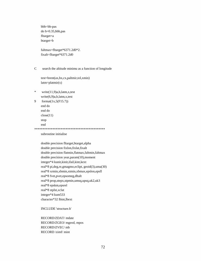
bbb=bb-pas do b=0.35,bbb,pas fltarget=a btarget=b faltmax=fltarget*6371.2d0*2. fixalt=fltarget*6371.2d0 C search the altitude minimu as a function of longitude test=brent(ax,bx,cx,paltmir,tol,xmin) latm=platmir(x) * write(11,9)a,b,latm,x,test write(6,9)a,b,latm,x,test 9 format(1x,5(F15.7)) end do end do close(11) stop end ******************************************* subroutine initialise double precision fltarget,btarget,alpha double precision fixlon,fixlat,fixalt double precision flatmin,flatmax,faltmin,faltmax double precision year,param(10),moment integer*4 kunit,kinit,ifail,kint,kext real*8 pi,deg,re,gmagmo,eclipt, geoid(3),uma(30) real*8 xrmin,xbmin,xtmin,xbmax,epslon,epsfl real*8 fvet,pvet,epsomeg,dltalt real*8 prop,stepx,stpmin,umsq,upsq,uk2,uk3 real*8 epskm,epsrel real*8 stplst,xclat integer*4 kum533 character*32 lbint,lbext INCLUDE 'structure.h' RECORD/ZDAT/ mdate RECORD/ZGEO/ mgeod, mpos RECORD/ZVEC/ mb RECORD /zimf/ mint

72

RECORD /zsun/ msun RECORD /zemf/ mext COMMON/mom/moment COMMON/FIXED/fixlon,fixlat,fixalt COMMON/LIMIT/flatmin,flatmax,faltmin,faltmax COMMON/BLCOR/fltarget,btarget COMMON/PITCH/alpha COMMON/UC160/ pi,deg,re,gmagmo,eclipt,geoid,uma COMMON/UC140/ mint,mext,msum COMMON/UC192/xrmin,xbmin,xtmin,xbmax,epslon,epsfl,fvet,pvet, * epsomeg,dltalt COMMON/UC190/prop,stepx,stpmin,umsq,upsq,uk2,uk3,epskm,epsrel, * stplst,xclat,kmflg,kum533 DATA kunit,kinit/0,1/ DATA kint,kext/0,0/ DATA year,param,alpha/1985.0d0,10*0.0d0,90.0d0/ flatmin=20.0d0 flatmax=-65.0d0 faltmin=6371.2d0*.9d0 fixlon=0.0d0 fixlat=0.0d0 mdate.iyear=1985 mdate.imonth=1 mdate.iday=1 mdate.ihour=0 mdate.imin=0 mdate.secs=0.0d0 C Initialize UNILIB library CALL UT990 (kunit, kinit, ifail) C modified values of several parameters in UNILIB common block xbmin=0.00000001 kum533=-1 xrmin=0.1 xbmax=100000000. xtmin=cos(6.*deg)

73

prop=0.02 stepx=0.02 C set geomagnetic field models (internal) CALL UM510 (kint, year, lbint, kunit, ifail) IF( ifail .LT. 0 )STOP C for centered and aligned dipole remove comments * mint.norder = 2 * mint.label = 'Dipolar magnetic field ' * mint.coef(2,1) = mint.gmmo * 1.0d+05 * mint.coef(1,2) = 0.0d+00 * mint.coef(2,2) = 0.0d+00 * mint.elong = 0.0d+00 * mint.colat = 0.0d+00 C Julian day CALL UT540(mdate) C set geomagnetic field models (external) CALL UM520 (kext, mdate.amjd, param, + lbext, kunit, ifail) IF( ifail .LT. 0 )STOP return end ************************************************** **** computation of the MacIlwain paramewter L**** double precision function alcoor(alt,alon,alat) double precision alt,alon,alat,alpha double precision fbm,flm,fks,fs,fsm,fbeq integer*4 nfmb,ifail,noprint,iifail real*8 pi,deg,re,gmagmo,eclipt, geoid(3),uma(30) real*8 xrmin,xbmin,xtmin,xbmax,epslon,epsfl real*8 fvet,pvet,epsomeg,dltalt real*8 prop,stepx,stpmin,umsq,upsq,uk2,uk3 real*8 epskm,epsrel real*8 stplst,xclat integer*4 kum533 INCLUDE 'structure.h'

74

RECORD/ZDAT/ mdate RECORD/ZGEO/ mgeod, mpos RECORD/ZVEC/ mb RECORD /zimf/ mint RECORD /zsun/ msun RECORD /zemf/ mext COMMON/PITCH/alpha COMMON/FLAG220/iifail COMMON /UC160/ pi,deg,re,gmagmo,eclipt,geoid,uma COMMON/UC140/ mint,mext,msum COMMON/UC192/xrmin,xbmin,xtmin,xbmax,epslon,epsfl,fvet,pvet, * epsomeg,dltalt COMMON/UC190/prop,stepx,stpmin,umsq,upsq,uk2,uk3,epskm,epsrel, * stplst,xclat,kmflg,kum533 nfbm=1 noprint=-1 mgeod.radius=alt mgeod.colat=90.0d0-alat mgeod.elong=alon C for centered and aligned dipole remove comment * gmagmo=mint.gmmo CALL UL220(mgeod,alpha,nfbm,fbm,flm,fkm,fsm,fbeq,fs,ifail) if(ifail.lt.0)then iifail=ifail print*,'ifail220 = ',ifail,'long = ',mpos.elong,mpos.colat,mpos.radius endif alcoor=flm return end ******************************************************************** C calculation of the geomagnetic field vector double precision function afield(al,alo,ala) implicit double precision (a-z) double precision al,alo,ala,bpos real*8 pi,deg,re,gmagmo,eclipt, geoid(3),uma(30) real*8 xrmin,xbmin,xtmin,xbmax,epslon,epsfl real*8 fvet,pvet,epsomeg,dltalt real*8 prop,stepx,stpmin,umsq,upsq,uk2,uk3

75

real*8 epskm,epsrel real*8 stplst,xclat integer*4 kum533 integer*4 ifail INCLUDE 'structure.h' COMMON/UC192/xrmin,xbmin,xtmin,xbmax,epslon,epsfl,fvet,pvet, * epsomeg,dltalt COMMON/UC190/prop,stepx,stpmin,umsq,upsq,uk2,uk3,epskm,epsrel, * stplst,xclat,kmflg,kum533 COMMON /UC160/ pi,deg,re,gmagmo,eclipt,geoid,uma COMMON/UC140/ mint,mext,msum COMMON/BVAL/bpos RECORD/ZDAT/ mdate RECORD/ZGEO/ mgeod, mpos RECORD/ZVEC/ mb RECORD /zimf/ mint RECORD /zsun/ msun RECORD /zemf/ mext mgeod.radius=al mgeod.colat=90.0d0-ala mgeod.elong=alo *********** evaluate magnetic feild*********** CALL UM530 (mgeod,mb,ifail) if (ifail.lt.0)then print*,'ifailUM530 = ',ifail endif bpos=mb.dnrm afield=mb.dnrm return end ********************************************************************* ************************************************************ C this function reduces the alcoor function that depends on C three variables into a function of only one variable, the altitude double precision function alcalt(alti) double precision alti double precision fixlon,fixlat,fixalt double precision fltarget,btarget,alpha COMMON/FIXED/fixlon,fixlat,fixalt COMMON/BLCOR/fltarget,btarget

76

alcalt=(alcoor(alti,fixlon,fixlat)/fltarget)-1.0d0 return end ************************************************** C this function reduces the afield function that depends on C three variables into a function of only one variable, the altitude double precision function afalt(alti) double precision alti double precision fixlon,fixlat,fixalt double precision fltarget,btarget,alpha COMMON/FIXED/fixlon,fixlat,fixalt COMMON/BLCOR/fltarget,btarget afalt=(afield(alti,fixlon,fixlat)/btarget)-1.0d0 return end ******************************************************************** C This function allows to find the zero of an other function C double precision function fzero(gfun,xmin,xmax,ep) double precision function gfun double precision xmin,xmax,ep,ecart,xup,xlow,xmean integer max,nbr xlow = xmin xup = xmax max = 1000 nbr = 0 ecart = dabs(xup-xlow) do while ((ecart.gt.ep) .and. (nbr .lt. max)) nbr = nbr + 1 xmean = (xup+xlow)/2. var = gfun(xlow)*gfun(xmean) if (var .lt. 0) then xup = xmean else xlow = xmean endif ecart = dabs(xup-xlow) * print*,xlow,xmean,xup,gfun(xlow),gfun(xmean) end do fzero = xmean return

77

end ******************************************************************** C This function allows to find the zero of an other function C It is exactely the same function as the previous fzero one C It's utility remains in the fact that fortran is not a redundant c language double precision function gzero(gfun,xmin,xmax,ep) double precision function gfun double precision xmin,xmax,ep,ecart,xup,xlow,xmean integer max,nbr xlow = xmin xup = xmax max = 1000 nbr = 0 ecart = dabs(xup-xlow) do while ((ecart.gt.ep) .and. (nbr .lt. max)) nbr = nbr + 1 xmean = (xup+xlow)/2. var = gfun(xlow)*gfun(xmean) if (var .lt. 0) then xup = xmean else xlow = xmean endif ecart = dabs(xup-xlow) * print*,xlow,xmean,xup,gfun(xlow),gfun(xmean) end do gzero = xmean return end ******************************************************************** C This function searches after the location where the computed B C is equal to the B target given in the introduction part. function dist(flat) implicit double precision (a-z) integer*4 nfmb,ifail,noprint,iifail double precision fbm,flm,fks,fs,fsm,fbeq INCLUDE 'structure.h' COMMON/BLCOR/fltarget,btarget COMMON/LIMIT/flatmin,flatmax,faltmin,faltmax COMMON/FIXED/fixlon,fixlat,fixalt COMMON/ALTI/alt1

78

RECORD/ZGEO/ mgeod, mpos COMMON/FLAG220/iifail external alcalt external afalt eps = 0.001 alpha=90. pi=4.*atan(1.) fixlat = flat C alt1 is the altitude where B=Btarget alt1 = fzero(afalt,faltmin,faltmax,eps) C C C Compute the L value with the altitude where B=Btarget bb = alcoor(alt1,fixlon,flat) C check if computed value of L matches Ltarget dist=bb/fltarget-1.0d0 return end ******************************************************************** C At a given longitude, this function finds the latitude mirror point by C searching the zero of the function dist(latitue) c between two latitudes (-65 and 40 degrees) function platmir(flon) implicit double precision (a-z) integer*4 nfmb,ifail,noprint,iifail double precision fbm,flm,fks,fs,fsm,fbeq INCLUDE 'structure.h' COMMON/BLCOR/fltarget,btarget COMMON/LIMIT/flatmin,flatmax,faltmin,faltmax COMMON/FIXED/fixlon,fixlat,fixalt RECORD/ZGEO/ mgeod, mpos COMMON/FLAG220/iifail COMMON/ALTI/alt1 external dist eps = 0.001 alpha=90. pi=4.*atan(1.)

79

fixlon = flon lmin = -65. lmax = 40. platmir = gzero(dist,lmin,lmax,eps) return end ************************************************ C At a given longitude, this function finds the altitude mirror point by C searching the zero of the function dist(latitue) c between two latitudes (-65 and 40 degrees) function paltmir(flon) implicit double precision (a-z) integer*4 nfmb,ifail,noprint,iifail double precision fbm,flm,fks,fs,fsm,fbeq INCLUDE 'structure.h' COMMON/BLCOR/fltarget,btarget COMMON/LIMIT/flatmin,flatmax,faltmin,faltmax COMMON/FIXED/fixlon,fixlat,fixalt RECORD/ZGEO/ mgeod, mpos COMMON/FLAG220/iifail COMMON/ALTI/alt1 external dist eps = 0.001 alpha=90. pi=4.*atan(1.) fixlon = flon lmin = -65. lmax = 40. p = gzero(dist,lmin,lmax,eps) paltmir=alt1 return end ****************************************************$ C Brent's method see part 10.2 Numerical recipes double precision function brent(ax,bx,cx,paltmir,tol,xmin) integer imax real*8 ax,bx,cx,paltmir,tol,xmin,cgold,eps external paltmir parameter (imax=100,cgold=.3819660,eps=1.0e-2) integer iter

80

real*8 a,b,d,e,etemp,fu,fv,fw,fx,p,q,r,tol1,tol2,u,v,w,x,xm common/minimum/x a=min(ax,cx) b=max(ax,cx) v=bx w=v x=v e=0. fx=paltmir(x) fv=fx fw=fx do iter=1,imax xm=0.5*(a+b) tol1=tol*abs(x)+eps tol2=2.*tol1 if(abs(x-xm).le.(tol2-.5*(b-a))) goto 3 if (abs(e).gt.tol1) then r=(x-w)*(fx-fv) q=(x-v)*(fx-fw) p=(x-v)*q-(x-w)*r q=2.*(q-r) if(q.gt.0.) p=-p q=abs(q) etemp=e e=d if(abs(p).ge.abs(.5*q*etemp).or.p.le.q*(a-x) * .or.p.ge.q*(b-x)) goto 1 d=p/q u=x+d if(u-a.lt.tol2.or.b-u.lt.tol2) d=sign(tol1,xm-x) goto 2 endif 1 if (x.ge.xm)then e=a-x else e=b-x endif d=cgold*e 2 if(abs(d).ge.tol1) then u=x+d else u=x+sign(tol1,d) endif fu=paltmir(u) if(fu.le.fx)then

81

if(u.ge.x)then a=x else b=x endif v=w fv=fw w=x fw=fx x=u fx=fu else if(u.lt.x)then a=u else b=u endif if(fu.le.fw.or.w.eq.x)then v=w fv=fw w=u fw=fu else if(fu.le.fv.or.v.eq.x.or.v.eq.w)then v=u fv=fu endif endif enddo 3 xmin=x brent=fx return end

82