experimental and analytical study of helical cross-flow...
TRANSCRIPT
Experimental and Analytical Study of Helical Cross-Flow Turbines for a Tidal Micropower Generation System
Adam L. Niblick
A thesis
submitted in partial fulfillment of the
requirements for the degree of
Master of Science in Mechanical Engineering
University of Washington
2012
Committee:
Brian Polagye
Alberto Aliseda
Brian Fabien
Program Authorized to Offer Degree:
Department of Mechanical Engineering
University of Washington
Abstract
Experimental and Analytical Study of Helical Cross-Flow Turbines for a Tidal Micropower Generation System
Adam L Niblick
Chair of the Supervisory Committee:
Doctor Brian Polagye Department of Mechanical Engineering
This study investigates the feasibility of a micro-scale tidal hydrokinetic generator to power autonomous
oceanographic instrumentation, with emphasis on turbine design and performance. This type of “micropower”
system is intended to provide continuous power on the order of 20 Watts. System components are reviewed
and include turbine, electrical generator, gearbox, controller, converter, and battery bank. A steady-state model
predicts system energy storage and power output in a mixed, mainly semidiurnal tidal regime with peak currents
of 1.5 m/s. Among several turbine designs reviewed, a helical cross-flow turbine is selected, due to its self-start
capability, ability to accept inflow from any direction, and power performance. Parameters impacting helical
turbine design include radius, blade profile and pitch, aspect ratio, helical pitch, number of blades, solidity ratio,
blade wrap ratio, strut design, and shaft diameter. The performance trade-offs of each are compared. A set of
three prototype-scale turbines (two three-bladed designs, with 15% and 30% solidity, and a four-bladed design
with 30% solidity and higher helical pitch) and several strut and shaft configurations were fabricated and tested
in a water flume capable of flow rates up to 0.8 m/s. Tests included performance characterization of the
rotating turbines from freewheel to stall, static torque characterization as a function of azimuthal angle,
performance degradation associated with inclination angles up to 10° from vertical, and stream-wise wake
velocity profiles. A four-bladed turbine with 60° helical pitch, 30% solidity, and circular plate “end cap”
provided the best performance; this design attained efficiency of 24% in 0.8 m/s flow and experienced smaller
performance reductions for tilted orientations relative to other variants. Maximum turbine efficiency increased
with increased flume velocity. A free-vortex model was modified to simulate the helical turbine performance.
Model results were compared to experimental data for various strut design and inflow velocities, and
performance was extrapolated to higher flume velocities and a full-scale turbine (0.7 m2 relative to 0.04 m2 in
flume tests). The model predicts experimental trends correctly but deviates from experimental values for some
conditions, indicating the need for further study of secondary effects for a high chord-to-radius ratio turbine.

i
TABLE OF CONTENTS LIST OF FIGURES ........................................................................................................................................... iii LIST OF TABLES .............................................................................................................................................. v ACKNOWLEDGEMENTS ............................................................................................................................ vi 1 Introduction .................................................................................................................................................. 1
1.1 Tidal Energy Potential ......................................................................................................................... 1 1.2 Tidal Theory........................................................................................................................................... 3 1.3 Local Resource for a Proposed Micropower Installation Site ..................................................... 5 1.4 Motivation for Micropower ................................................................................................................ 6 1.5 Existing Tidal Micropower Technology .......................................................................................... 8 1.6 Tidal Micropower System Components .......................................................................................... 9
1.6.1 Turbine .......................................................................................................................................... 10 1.6.2 Generator...................................................................................................................................... 11 1.6.3 Gearbox ........................................................................................................................................ 13 1.6.4 Battery Bank ................................................................................................................................. 14 1.6.5 Controller/Converter ................................................................................................................. 16 1.6.6 Loads ............................................................................................................................................. 17
1.7 System Performance Model .............................................................................................................. 18 2 Turbine Selection ........................................................................................................................................ 25
2.1 Turbine Performance Parameters ................................................................................................... 25 2.2 Turbine Types ..................................................................................................................................... 26
2.2.1 Savonius Rotor ............................................................................................................................ 28 2.2.2 Darrieus Turbines ....................................................................................................................... 29 2.2.3 Hybrid Turbines .......................................................................................................................... 32 2.2.4 Helical (Gorlov) Turbine ........................................................................................................... 33
2.3 Helical Tidal Turbine Design Parameters ...................................................................................... 34 2.3.1 Blade Profile ................................................................................................................................. 34 2.3.2 Solidity Ratio and Chord-to-Radius Ratio ............................................................................. 36 2.3.3 Number of blades ....................................................................................................................... 37 2.3.4 Aspect Ratio ................................................................................................................................. 37 2.3.5 Helical Pitch Angle ..................................................................................................................... 38 2.3.6 Blade Pitch Angle and Mount Point Ratio ............................................................................ 39 2.3.7 Blade Wrap ................................................................................................................................... 42 2.3.8 Design Trade-Offs ...................................................................................................................... 43 2.3.9 Blade Attachment ....................................................................................................................... 44 2.3.10 Strut Design ............................................................................................................................... 44 2.3.11 Central Shaft Design ................................................................................................................ 45
3 Vertical Axis Turbine Modeling ............................................................................................................... 46 3.1 Blade Element Analysis ..................................................................................................................... 46 3.2 Momentum Models ............................................................................................................................ 48 3.3 Vortex Model ....................................................................................................................................... 49 3.4 CFD Models ........................................................................................................................................ 53 3.5 Secondary Effects ............................................................................................................................... 53
3.5.1 Pitch Rate...................................................................................................................................... 54 3.5.2 Dynamic Stall ............................................................................................................................... 54 3.5.3 Flow Curvature ............................................................................................................................ 56
3.6 Model Implementation ...................................................................................................................... 58 4 Experimental Testing ................................................................................................................................. 59
4.1 Test Purpose ........................................................................................................................................ 59 4.2 Experimental Turbine Designs ........................................................................................................ 59
4.2.1 Turbine Design Parameters ...................................................................................................... 60
ii
4.2.2 Manufacturing and Construction ............................................................................................ 62 4.3 Flume Test Setup and Turbine Installation ................................................................................... 62 4.4 Instrumentation ................................................................................................................................... 64 4.5 Test Methodology ............................................................................................................................... 65
4.5.1 General Test Procedure ............................................................................................................. 66 4.5.2 Specific Test Descriptions......................................................................................................... 67 4.5.3 Instrument and Data Accuracy ................................................................................................ 71 4.5.4 Blockage Correction ................................................................................................................... 73
4.6 Test Results for Baseline Configuration ........................................................................................ 75 4.6.1 Load Performance Test ............................................................................................................. 75 4.6.2 Static Torque ................................................................................................................................ 78 4.6.3 Tilted Turbine Test ..................................................................................................................... 83 4.6.4 Start-up and Shut-Down Test .................................................................................................. 84 4.6.5 Turbine Wake .............................................................................................................................. 86
4.7 Design Considerations ....................................................................................................................... 89 4.7.1 Number of Blades and Helical Pitch ...................................................................................... 89 4.7.2 Strut Geometry ............................................................................................................................ 91 4.7.3 Shaft Diameter............................................................................................................................. 93 4.7.4 Tilt Angle ...................................................................................................................................... 95 4.7.5 Solidity Comparison ................................................................................................................... 97
5 Vortex Model Results ................................................................................................................................ 99 5.1 Model Parameters ............................................................................................................................... 99 5.2 Modeling Strut and Interference Drag ......................................................................................... 102 5.3 Adaptations for a Helical Turbine ................................................................................................. 103 5.4 Prototype Turbine Modeling .......................................................................................................... 104
5.4.1 Model Prediction of Strut Drag Effects ............................................................................... 106 5.4.2 Model Prediction with Varying Inflow Velocity ................................................................ 107 5.4.3 Prediction of Prototype Turbine Performance at Higher Flow Speeds ........................ 108
5.5 Impact of Secondary Effects on Model Performance .............................................................. 110 5.6 Prediction of Performance of the Full-Scale Turbine ............................................................... 114 5.7 Summary ............................................................................................................................................. 116
6 Conclusions and Future Work ............................................................................................................... 117 6.1 Accomplishments and Conclusions .............................................................................................. 117 6.2 Future Work ...................................................................................................................................... 121
GLOSSARY OF SYMBOLS ......................................................................................................................... 124 REFERENCES................................................................................................................................................ 126 Appendix A: Prototype Turbine Manufacturing Details ........................................................................... 132 Appendix B: Test Setup and Instrumentation Details ............................................................................... 135 Appendix C: Additional Test Results and Tabular Data .......................................................................... 143 Appendix D: Blockage Analysis .................................................................................................................... 151 Appendix E: Momentum Models ................................................................................................................... 157 Appendix F: Cascade Model Methodology ................................................................................................. 165

iii
LIST OF FIGURES
Figure 1.1 Average Daily Maximum Tidal Range .................................................................................................. 2 Figure 1.2 Diurnal and Semidiurnal Tides ............................................................................................................... 4 Figure 1.3 Spring and Neap Tides ............................................................................................................................ 4 Figure 1.4 Sea Spider Research Tripod .................................................................................................................... 6 Figure 1.5 MNU Hybrid Turbine ............................................................................................................................. 8 Figure 1.6 Aquair UW ................................................................................................................................................. 9 Figure 1.7 New Energy Corporation 5 kW Power Generation System ............................................................ 9 Figure 1.8 Micropower System Block Diagram ................................................................................................... 10 Figure 1.9 Permanent Magnet Generators ............................................................................................................ 13 Figure 1.10 Micropower System Model ................................................................................................................. 19 Figure 1.11 Turbine-Generator Operating Curves .............................................................................................. 20 Figure 1.12 Micropower System Battery Energy Storage .................................................................................. 23 Figure 1.13 Micropower System Power Generation ........................................................................................... 24 Figure 2.1 Velocity and Force Vectors for an Airfoil ......................................................................................... 27 Figure 2.2 Axial Flow Tidal Turbine ...................................................................................................................... 28 Figure 2.3 Savonius Rotor Two-Stage Bucket and Diagram ............................................................................. 29 Figure 2.4 Sketches of Darrieus Turbine Designs ............................................................................................... 30 Figure 2.5 Diagram of Cross-Flow Turbine Velocity Vectors .......................................................................... 31 Figure 2.6 Helical (Gorlov) Turbine ....................................................................................................................... 33 Figure 2.7 Angle of Attack Sign Convention on a Cambered Airfoil ............................................................. 35 Figure 2.8 Asymmetrical Blade Profiles ................................................................................................................. 36 Figure 2.9 Aspect Ratio ............................................................................................................................................. 38 Figure 2.10 Helical Pitch Angle ............................................................................................................................... 39 Figure 2.11 Blade pitch Angle .................................................................................................................................. 40 Figure 2.12 Blade Mount Point at ¼-chord .......................................................................................................... 41 Figure 2.13 Blade Mount Point at ½-chord .......................................................................................................... 42 Figure 2.14 Turbine Blade Support Configurations ............................................................................................ 45 Figure 3.1 Bladed Element Velocity Vectors, Lift and Drag Forces ............................................................... 47 Figure 3.2 Normal and Tangential Forces............................................................................................................. 48 Figure 3.3 Vortex Model Blade Element ............................................................................................................... 50 Figure 3.4 Velocity Induced by a Vortex Filament ............................................................................................. 51 Figure 3.5 Lift and Drag Coefficient Variation in Dynamic Stall ..................................................................... 55 Figure 3.6 Velocity Vectors Resulting in Apparent Flow Curvature ............................................................... 57 Figure 4.1 Water Flume Test Channel ................................................................................................................... 62 Figure 4.2 Test Frame, Instrumentation Module, and Turbine ........................................................................ 63 Figure 4.3 Test Setup Stream-Wise View .............................................................................................................. 64 Figure 4.4 Test Instrumentation Module .............................................................................................................. 65 Figure 4.5 Acoustic Doppler Velocimeter ............................................................................................................ 65 Figure 4.6 Test Setup for Tilted Turbine Test ..................................................................................................... 69 Figure 4.7 Instrumentation Output Sample for Performance and Static Tests ............................................ 72 Figure 4.8 Baseline Turbine Configuration ........................................................................................................... 75 Figure 4.9 Load Performance Curves for Baseline Configuration ................................................................... 77 Figure 4.10 Lift and Drag Coefficients for a NACA 0018 for Various AOA ............................................... 78 Figure 4.11 Static Torque Curve for Baseline Configuration ............................................................................ 79 Figure 4.12 Upstream View of Turbine with Respect to Static Torque ......................................................... 80 Figure 4.13 Single Blade Static Torque .................................................................................................................. 81 Figure 4.14 Comparison of Baseline Turbine Performance to Single Blade Superposition ....................... 82 Figure 4.15 Wake Effects on Turbine Static Torque .......................................................................................... 82 Figure 4.16 Turbine Tilt Angle Performance for Baseline Configuration ...................................................... 83 Figure 4.17 Start-up/Shutdown Test Data Profile .............................................................................................. 85

iv
Figure 4.18 Non-Dimensionalized Wake Velocity .............................................................................................. 88 Figure 4.19 Turbine Design Comparison Configurations ................................................................................. 89 Figure 4.20 Performance Comparison of Three- and Four-Bladed Turbines ............................................... 90 Figure 4.21 Static Torque Comparison of Three- and Four-Bladed Turbines .............................................. 91 Figure 4.22 Strut Design Comparison Configurations ...................................................................................... 92 Figure 4.23 Strut Design Performance Comparison ........................................................................................... 92 Figure 4.24 Shaft Design Comparison Configurations ...................................................................................... 94 Figure 4.25 Shaft Design Performance Comparison .......................................................................................... 94 Figure 4.26 Tilt Angle Performance Comparison ............................................................................................... 96 Figure 4.27 Maximum Power Coefficient as a Function of Flume Velocity ................................................. 97 Figure 4.28 Low Solidity Turbine ........................................................................................................................... 98 Figure 5.1 Model Convergence for Successive Revolutions ........................................................................... 100 Figure 5.2 Model Blade Segmentation and Endpoint Variation .................................................................... 104 Figure 5.3 Model Output Demonstrating Impact of Secondary Effects ...................................................... 105 Figure 5.4 Prototype Turbine Model Results for Different Mount Point Ratio ......................................... 106 Figure 5.5 Vortex Model Prediction of Strut Drag Effects ............................................................................. 107 Figure 5.6 Vortex Model Prediction for Varying Inflow Velocity ................................................................. 108 Figure 5.7 Prototype Turbine Model Extrapolation to Inflow Velocity of 1.5 m/s .................................. 110 Figure 5.8 Effect of Flow Curvature at High Tip Speed Ratio ....................................................................... 111 Figure 5.9 Angle of Attack Lag when Torque Coefficient is High ................................................................ 113 Figure 5.10 Angle of Attack Lag Shown on Static Lift and Drag Coefficient Curves ............................... 114 Figure 5.11 Full-Scale Turbine Model Predictions with All Secondary Effects Active ............................. 115 Figure 5.12 Full-Scale Model Predictions with Pitch Rate and Flow Curvature Disabled ....................... 116

v
LIST OF TABLES
Table 1.1 Battery Comparison Chart ...................................................................................................................... 15 Table 1.2 Micropower System Loads ..................................................................................................................... 18 Table 1.3 Tidal Constituent Parameters................................................................................................................. 20 Table 2.1 Helical Turbine Design Parameter Trade-Offs .................................................................................. 43 Table 4.1 Turbine Design Parameters .................................................................................................................... 60 Table 4.2 Test Matrix ................................................................................................................................................. 70 Table 4.3 Instrumentation Accuracy ...................................................................................................................... 71 Table 4.4 Turbine Dimensions and Flume Flow Parameters ........................................................................... 74 Table 4.5 Baseline Configuration Tilt Angle Comparison ................................................................................. 84 Table 4.6 Baseline Configuration Cut-In and Cut-Out Speeds ........................................................................ 86 Table 4.7 Power Coefficient Loss from Tilt Angle Prediction versus Actual ............................................... 97 Table 5.1 Model Geometric Inputs for Prototype and Full-Scale Turbines ................................................ 102

vi
ACKNOWLEDGEMENTS
I would like to thank the chair of my advisory committee, Dr. Brian Polagye, for all of the guidance and
insightful he provided on this project. He always made himself available to talk when needed, and his prompt
and helpful feedback to my numerous questions was much appreciated. I would also like to thank the other
members of my advisory committee, Drs. Alberto Aliseda and Brian Fabien, who provided valuable insight in
their areas of expertise when needed. I am very thankful to Dr. Roy Martin for generously providing the Roy
Martin Marine Fellowship, which provided the funds for much of my schooling and research. Also, I appreciate
Dr. Martin’s advice and guidance in the development of the test setup and instrumentation selection. Thank
you to Dr. Philip Malte for selecting me to receive the Roy Martin Marine Fellowship and for helping to secure
the funds for the laboratory test setup and for my second year of schooling.
Thank you to Bill Kuykendall, ME Lab Engineer, who provided the initial guidance for the laboratory
experimental setup and was always willing to provide advice with instrumentation problems. I also appreciate
the help from the machine shop supervisors Kevin Soderlund and Eamon McQuaide, who provided their
manufacturing expertise and assisted in manufacturing the helical turbines. Thanks to Dr. Jim Thomson and
the Applied Physics Laboratory for lending an Acoustic Doppler Velocimeter for use in flume testing. I am
grateful for the help of the capstone design team members, Nick Stelzenmuller, Bronwyn Hughes, Josh
Anderson, Celest Johnson, Leo Sutanto, and Brett Taylor for their input into the turbine designs and for their
work in building the flume test frame. Thank you to Matt Barone and Sandia National Laboratories for
providing the vortex model that was used as part of my work.
Thanks to all of my friends and colleagues in the Mechanical Engineering Department at the University of
Washington; we helped each other succeed, did some great research, and had fun along the way. Thanks to the
ME staff for all of their guidance and help with various issues.
Last, but certainly not least, I would like to thank my wife, Marie, for her love, patience and support during the
busy, stressful times of my Master’s program.
1
1 Introduction
This thesis provides a study of a helical hydrokinetic turbine for use in a tidal current to generate small-scale
electrical power for powering instrumentation loads. The term “micropower” refers to energy generation on the
average scale of O(20) W. Chapter 1 provides a brief overview of tidal energy theory, tidal micropower system
components, and results of a simple system simulation model. Chapter 2 focuses on the turbine types and
design parameters of importance for a tidal micropower system. Chapter 3 provides an overview of some of the
more popular numerical models for cross-flow tidal turbines. Chapter 4 gives experimental results of flume
testing of two helical tidal turbine prototypes. Several design parameters are compared in the tests to determine
best design. Finally, Chapter 5 provides a comparison between experimental results and the predictions of a
vortex model to evaluate experimental results and the model’s ability to accurately represent a high solidity, low
operating speed helical tidal turbine.
1.1 Tidal Energy Potential
Tidal energy is a form of renewable energy that is sourced from the gravitational pull of the Sun and the Moon
on the Earth’s oceans and seas. Unlike some other forms of renewable energy, such as solar and wind energy,
tidal currents are predictable within a reasonable level of certainty for several years into the future. The total
dissipation of energy by tides on Earth is estimated to be 3 TW, with the estimated combined total potential in
shallow, exploitable areas near 120 GW (Twidell & Weir, 2006). For comparison, the US yearly consumption of
power is near 430 GW (The World Factbook 2009). While intense tidal currents do not require large tidal
ranges, the two are often correlated and the “hot spots” shown in Figure 1.1 broadly correspond to areas with
hydrokinetic potential. According to the Electrical Power Research Institute (EPRI) site selection criteria, a
viable site for commercial power production normally requires peak currents of 1.5 m/s or greater (Hagerman
& Polagye, 2006), although Owen & Bryden (2007) suggest it may be as low as 1.0 m/s. For sites that meet this
criterion, there is great interest in collecting in-situ data to verify their suitability for tidal power extraction and
establish environmental baseline measurements.

2
Figure 1.1 Average Daily Maximum Tidal Range (Source: www.pacificstormsclimatology.org/images/glossary/tides.png)
Although tidal energy offers the advantages of renewability and predictability, it also comes with several
challenges:
Corrosion, fouling and biofouling can lead to device performance degradation and frequent
maintenance requirements;
Interaction with marine fauna can lead to alteration of behavior, injury, or mortality;
Alterations in tidal range, noise levels and sediment transport can alter ecosystems;
Development and installation of a tidal power extraction facility can temporarily disrupt or alter human
activity, the marine environment and nearby landscapes;
Competition with existing users (e.g. fishing industry, shipping) for the area of desired installation;
Micro-siting considerations can significantly affect the power output of a tidal turbine (Polagye and
Thomson, submitted);
Logistical challenges associated with accessibility of remote sites for research, installation and
maintenance of tidal devices.
Due to these engineering, environmental, and societal challenges, hydrokinetic tidal power extraction on a
commercial scale is still in development. However, increasing global energy demand and recognition of the
finite limit of fossil fuel availability has encouraged recent work in both studying the characteristics of potential
tidal energy sites and in developing large scale tidal power generation schemes.

3
1.2 Tidal Theory
Tidal theory in this section follows the explanation given by Twidell & Weir (2006). A balance of gravitational
and centrifugal forces maintains the distance of the Sun, the Moon and the Earth. These forces are also
responsible for the generation and movement of the tides. Several astronomical phenomena contribute to the
tidal cycle. The strongest factor in tidal range is due to the gravitational pull of the Moon. When the Moon is
located at the Earth’s equatorial plane, the waters of the Earth’s oceans tend to congregate at the point nearest
to and farthest from the Moon. The point on the Earth nearest the Moon experiences greatest gravitational
attraction, but a smaller centrifugal force, since it is closer to the center of mass of the Moon-Earth system. The
point farthest away from the Moon experiences the greatest centrifugal force but the lowest gravitational force.
Solid material on the Earth’s surface experiences this force but is held in position with minimum deformation.
The liquid water on the Earth’s surface, however, is free to move and tends to congregate in a tidal bulge at the
points of greatest force. The motion of the tides are caused by the Earth’s rotating relative to the Moon and
changing the locations of greatest force concentration.
If the Moon stayed on the Earth’s equatorial plane, then the waters of the world would experience a tidal period
with a frequency of twice the mean lunar day, or one peak every 12 hours, 25 minutes. This tidal character does,
in fact, occur in many locations to a greater or lesser extent and is known as a semidiurnal tide. However, the
Moon does not always remain on the Earth’s equatorial plane, and in such cases that it moves toward the poles,
a tidal period with frequency of once during the mean lunar day occurs. This is known as a diurnal tide and
occurs once every 24 hours, 50 minutes. Tidal currents are classified into groups based on the ratio of diurnal to
semidiurnal constituent amplitude: mainly diurnal, mainly semidiurnal, or mixed. Mixed tides are classified
either into mixed, mainly semidiurnal or mixed, mainly diurnal. Figure 1.2 provides a simple illustration of the
diurnal and semidiurnal tides.

4
Figure 1.2 Diurnal and Semidiurnal Tides (Source: co-ops.nos.noaa.gov/restles4.html)
The tidal component due to the action of the Sun is similar to that of the Moon, but its strength is only about
45% of that of the Moon. When the Moon, Sun, and Earth are aligned, which occurs twice every synodic lunar
month, or 14.765 days, the tidal range is greatest. This is known as a spring tide. Conversely, when the Sun,
Earth and Moon are in quadrature, again occurring every 14.765 days, a neap tide occurs with the smallest tidal
range. A diagram depicting neap and spring tides is shown in Figure 1.3.
Figure 1.3 Spring and Neap Tides (Source: co-ops.nos.noaa.gov/restles3.html)

5
Additionally, tides are affected by the oscillation of the Earth-Moon separation distance at a frequency of 27.55
days. At apogee, when the distance is greatest, the tidal range will be smallest, due to lower lunar gravitational
force. In contrast, tidal range is greatest at perigee, when the Earth-Moon separation is lowest.
Other factors, such as lagging of the tide relative to the Moon’s motion, lesser astronomical factors, local
bathymetry and topography, and non-tidal forces such as density stratification, all contribute to the tidal range
and current in a specific locale. The tidal range is minimal in open oceans and becomes greater near coastal
areas where local topography and bathymetry amplifies the range (Epler, 2010).
To relate the tidal current velocity to the power of the resource, the kinetic power density is used. The kinetic
power density, or power per unit area, of the current, is given by Equation (1.1):
, (1.1)
where is the density of water (nominally 1024 kg/m3 for seawater) and is the velocity of the stream-wise
flow (Polagye, 2011). The kinetic power density provides a measure of the amount of power that could be
extracted per unit area from a hydrokinetic resource if the power could be extracted at 100% efficiency. It is a
useful measure for the determining the capability of the resource, although 100% efficient conversion to
electricity is not practical.
1.3 Local Resource for a Proposed Micropower Installation Site
One proposed tidal power location of interest is Admiralty Inlet, the northern entrance to Puget Sound in the
US state of Washington. Under a grant from the US Department of Energy, the Northwest National
Renewable Energy Center at the University of Washington is collecting and analyzing data about the existing
environment of the proposed site, prior to installation of a pilot-scale installation of a tidal turbine power
extraction device.
Admiralty Inlet is a constricted channel approximately 5 km across and 60 m deep, separating the Strait of Juan
de Fuca from Puget Sound (Epler, 2010). The narrow channel depth separates the larger, deeper water bodies
(Puget Sound has a maximum depth around 280 m). During each ebb and flood tide, the entire tidal prism
(difference in volume between high and low tide) of Puget Sound passes through Admiralty Inlet (excepting a
small exchange through Deception Pass). Due to the relatively small cross-sectional area of Admiralty Inlet,
velocities up to 3 m/s occur in the channel compared to tidal velocities near Seattle, which are closer to 0.2 m/s.
The tidal regime in Admiralty Inlet is classified as mixed, mainly semi-diurnal. The seabed is fairly flat and
dominated by small cobbles (smaller sediments having been scoured away by strong tidal currents).

6
1.4 Motivation for Micropower
As discussed in Section 1.1, sites with peak current velocities of at least 1.5 m/s may be viable for tidal power
extraction. Field data collection activity follows site identification to determine viability. Often field
measurements must be made on a long-term basis in a remote, off-shore location that precludes the full-time
presence of research personnel. In such cases the field instruments must reliably operate for long periods of
time without interruption or human interaction. For example, in studying Admiralty Inlet, the University of
Washington uses a Sea Spider instrumentation package, measuring roughly 1.25 meters wide by 0.68 meters
height and instrumented with various measuring equipment, including the following:
Acoustic Doppler current profiler (ADCP) – measures water column velocity from the Doppler shift of
backscattered acoustic pulses transmitted from the ADCP;
CTDO sensor – measure conductivity, temperature, depth and dissolved oxygen levels;
C-POD/T-POD hydrophones - record echolocation acoustic signals by cetaceans (principally harbor
porpoise);
Broadband hydrophones – record ambient noise generated by ferry and shipping traffic, marine
mammals, and cobble movement on the seabed;
Sediment trap – characterize sediment advected through the site;
Fish tag receiver – monitor any tagged fish species using or transiting through the site;
Buoy and acoustic release – for retrieving the Sea Spider.
Figure 1.4 Sea Spider Research Tripod
Some of the instrumentation, including the ADCP, hydrophones, CTDO, and CPOD/TPOD, require a small
amount of electric power to operate. The instruments are deployed on the bottom-lander Sea Spider in depths
of up to 60 m for durations of up to six months to collect oceanographic data that characterizes the physical and

7
biological environment. Currently, this requires a large volume of single-use batteries to power the
instrumentation. Data storage capabilities are often limited to low power options (e.g., compact flash cards) to
maintain power throughout the duration of the deployment. If instrumentation power could be generated on-
site, this would allow for greater flexibility in device deployments and instrumentation. These factors, and also
the cost associated with the batteries and the negative environmental connotation associated with their single
use and disposal, motivates interest in alternative forms of power supply.
Unfortunately, water depth and tidal currents preclude the use of an off-grid power system utilizing solar, wave,
or wind power. Economic realities also preclude a grid connection. However, tidal power is a readily available
local renewable energy source. Admiralty Inlet, with current velocities up to 3 m/s, is an ideal location for
installation of a pilot micropower system.
In addition to minimum resource requirements, a tidal hydrokinetic micropower system would need to meet the
following requirements to be considered a viable alternative to a battery-powered system:
The system must generate sufficient power to continuously power equipment for the duration of
deployment, using energy storage to buffer against tidal intermittency (i.e., ebb/flood and neap/spring
cycles);
An instrumentation package with integrated energy harvesting must be compact to allow for
deployment using existing methods (e.g., from a research vessel with A-frame and winch);
The electrical /electronic portions of the system must be watertight;
The turbine must operate with flow from any horizontal direction to accommodate deployments where
the azimuthal positioning is not possible or platform rotation after deployment is likely (e.g., Sea
Spiders, as discussed in Polagye and Thomson (submitted));
Turbine performance should not be significantly degraded with tilt angles up to 10 degrees to
accommodate moderate seabed slopes.
Although only Admiralty Inlet is mentioned as a possible deployment site, tidal micropower systems could be
deployed in any location with sufficient kinetic resources. Also, other deployment scenarios are possible and
include a moored deployment, suspension from a floating barge or buoy, or deployment from a dock on a river.
It is important to note that some care must be taken with integration of the micropower system so as not to
degrade the quality of the field measurements. Near-field flow velocities may be affected by vibration from
rotation of the turbine. Also, noise associated with turbine motion and the generator will be recorded by a
hydrophone and would contaminate an unknown number of frequency bands when the turbine is in operation.
In some cases, micropower may not be compatible with all desired measurements. Conversely, some
measurements, such as long-term observations with multi-beam sonars, would not be possible without
micropower due to high power consumption relative to battery capacities.

8
1.5 Existing Tidal Micropower Technology
Some tidal micropower designs already exist in development or are available commercially. The Memorial
University of Newfoundland (MNU), for example, is performing research into a twisted Savonius rotor, a multi-
stage Savonius rotor, and a combined Darrieus-Savonius (Alam & Iqbal, 2009) hybrid turbine (shown below).
The intended use is to power seismic activity monitors off the coast of Newfoundland, Canada. Expected
current velocities in the intended deployment location off the Atlantic Coast are very low, averaging 0.5 m/s
(Khan, 2008). Given the expected rotor efficiencies of ~20%, maintaining a power output of 20 W would be
challenging.
Figure 1.5 MNU Hybrid Turbine (Source: Alam, 2009)
Some hydrokinetic turbine devices exist that are designed to be installed on the back of a moving, seagoing
vessel. The Ampair Aquair Underwater 100 is a horizontal axis turbine with 312 mm diameter rotor with
integrated, waterproof generator, and is designed to provide 24 W power in a 2 m/s current (Ampair Energy
Ltd, 2010). The device could conceivably be designed to operate in a tidal current scenario but would need a
method to yaw it to the direction of current and is only rated for depths up to 10 meters (www.ampair.com).

9
Figure 1.6 Aquair UW (Source: www.ampair.com)
New Energy Corporation, LLC is marketing a 5 kW power generation system using a four-bladed Darrieus
rotor. The device, which measures 1.5 m diameter by 2.25 meters high, is more than twice the size of turbine
being considered in the present study. The rated power of 5 kW is for a 3 m/s current; the device produces less
than 1 kW in stream flows of 1.5 m/s (New Energy Corporation Inc, n.d.). It is designed to have its drive train
above the waterline.
Figure 1.7 New Energy Corporation 5 kW Power Generation System (Source: New Energy Corporation, Inc (n.d.))
1.6 Tidal Micropower System Components
A tidal micropower system consists of hydrokinetic tidal turbine, gearbox (optional), electrical generator, voltage
converter, battery bank, system controller, and system loads. These components are described in the sections to
follow. Critical to the successful integration of a micropower system is proper selection and characterization of
each of these system components. The components must be compatible with one another and must meet the
requirements for system installation and integration. Drive train and controller components must be designed
to be as compact as possible, while maintaining high efficiency. The components must be located so as to allow

10
for instrumentation to fit onto the module. A simple block diagram of the system is shown in Figure 1.8. In the
diagram, the thick black lines represent mechanical power transfer, the paired black lines represent electrical
power transfer, and the orange lines represent signals and communication.
Figure 1.8 Micropower System Block Diagram
The electromechanical system can be modeled either as a steady state system or in a more detailed manner with
transient response of system components included. Khan et al. (2010) created a dynamic system response model
for a micropower system with a grid tie, describing each component with a distinct system response function.
For a system model simulating maximum power point tracking control or for simulation of the system during
start-up or shutdown, a dynamic system response model is required. In the present study, however, the focus is
on the quasi-steady performance of the system, with the components operating in equilibrium. Therefore, in
the present system model (See Section 1.7), each component is modeled with its steady state response.
1.6.1 Turbine
The turbine converts hydrokinetic power into mechanical power. A number of different types of turbines or
rotors may be used for this purpose: drag or lift style devices, axial or cross-flow turbines, hybrid turbines
combining aspects of several variants, turbines with variable or fixed pitch blades, ducted turbines, etc. The
output from a turbine is normally a fixed-pitch shaft that is characterized by a torque and rotation rate. Several
turbine types are discussed in further detail in Section 2. Other, more novel, approaches to power take-off
include oscillating hydrofoils and linear motion for vortex-induced vibration.
The performance parameters of concern for a turbine in a micropower system are
+ -+ -
Loads
Monitoring Equipment
Controller/processor
Data storage
Gearbox
Generator
Tidal Turbine
Battery Bank
ConverterRectifier
Turbine
Controller
Loads

11
Device performance curves, which allows for determining system torque, power and rpm given inflow
velocity;
Starting torque and self-starting capability;
Torque oscillation during operation;
Performance degradation when subjected to non-ideal flow conditions, including off-axis flow, tilted
deployment relative to incoming flow, response to turbulence, response to unsteady conditions;
Structural loading and fatigue performance;
Susceptibility to biofouling and corrosion and resulting performance degradation (Orme et al., 2001).
The performance curves provide the general efficiency of the devices at different tip speed ratios. Operation at
higher tip speed ratio is a desirable characteristic for system integration, because it allows greater compatibility
with generator operating speeds and enables the possibility of a low gear ratio or a direct drive turbine. The
ability of the turbine to provide sufficient starting torque to self-start is a critical requirement, considering the
deployment will be in a remote location. Start-up torque supplied by onboard power would add complexity and
increase parasitic losses. Torque oscillation should be minimal to prevent oscillation in power output and fatigue
of components. Biofouling and corrosion can be in part mitigated by appropriate material selection and marine
coatings.
The present study focuses primarily on developing information about the first four bullets given above.
1.6.2 Generator
A generator converts the mechanical power output from the turbine (or gearbox) to electrical power.
Commonly, a changing magnetic field induces an electric current through the generator’s armature through
Faraday’s law. The output of the generator can be either alternating current (AC) or direct current (DC)
depending on design.
The main difficulty with integrating a small hydrokinetic turbine with an electric generator is torque-rpm
matching. Often, generator peak operating efficiency is at a much higher rpm than the rotation rate
corresponding to peak efficiency of the turbine. For example, peak efficiency of a three-bladed helical turbine
tested by Shiono et al. (2002) occurs at 100 rpm with corresponding torque of 2.1 Nm. The Windblue Power
DC-540 Permanent Magnet DC generator, on the other hand, has optimum efficiency of ~65% at speeds of
490 rpm or greater and with torque 1.7 Nm or higher, while its efficiency at 100 rpm is just ~35% (D. Sutton,
Windblue Power, personal communication, 24 January 2011). Obviously, a direct drive system using these two
components creates a mismatch, resulting in a very low overall system efficiency and poor power output. This
can be addressed with a speed-increasing gearbox. However, the gearbox introduces an additional power loss to
the system and can decrease system reliability; especially for a gearbox with multiple gear stages. Given the low
12
power and torque output of a small hydrokinetic turbine, with efficiency likely less than 40%, useful power
generation is contingent upon adequate drive train efficiency requirements.
Three basic types of electrical generators include induction generators, synchronous generators, and direct
current (DC) generators. Under these main generator types, several sub-types exist: field-excited, permanent
magnet, single or polyphase alternating current (AC) or direct current (DC) output, axial or radial flux, stepper
motors, etc. However, for a generator integrated into a micropower system, specific system attributes are
desired that limit generator options. A permanent magnet field is required to avoid using stored electrical energy
to generate a magnetic field, and in a remote application, grid-power is obviously not available to provide field
excitation. DC power output is required to charge the batteries, although the generator can have an AC output
that is rectified to DC. The rectification may be internal to the generator or may be a separate converter. An
ideal generator for a micropower system would also have the following characteristics: a low starting torque to
facilitate easy turbine startup; a high, constant efficiency performance over a wide range of operating speeds; and
low rpm operation to enable direct drive of the system or to keep the gear ratio low.
Induction motors historically have been rarely used as generators, but have become popular generators for use
in commercial wind power applications due to simple design and ability to run at a constant frequency for grid
integration (Fitzgerald et al., 2003). Induction motors are less useful for a micropower application. The
induction generator stator requires AC field excitation and the rotor must be rotated just above the synchronous
speed. Also, since the desired output is DC there is no benefit to an induction motor’s constant frequency AC
output. Of the remaining two motor types, three specific generator configurations are considered:
Permanent magnet radial flux DC generator;
Permanent magnet radial flux alternator (AC synchronous generator) with rectified DC output;
Permanent magnet axial flux generator (rectified synchronous or DC).
The radial flux DC generator and alternator are commonly available motors that are frequently used in small-
scale wind power generation systems. Many of the alternator-type generators are automotive alternators that are
rewound for wind power applications and thus are fairly inexpensive off-the-shelf products. The devices,
however, are fairly inefficient and operate at rpm well above that of a hydrokinetic turbine. A gearbox would be
required to step up the rotation rate of the turbine output, at the expense of the system efficiency.
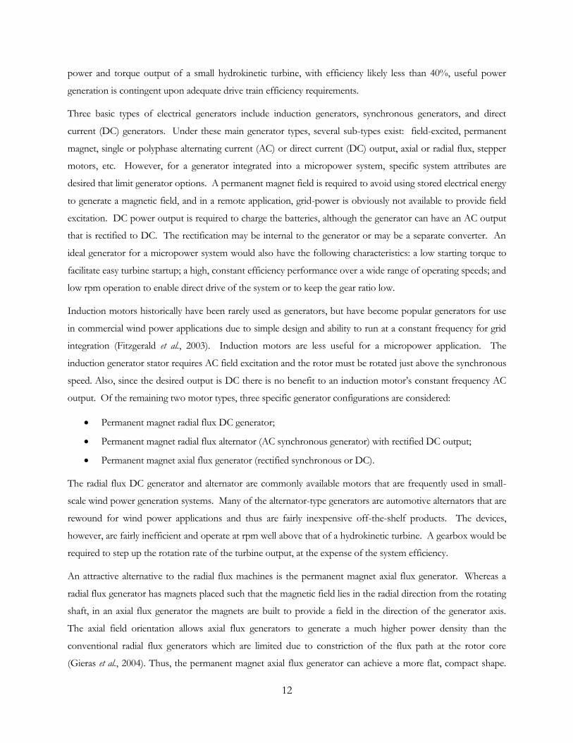
An attractive alternative to the radial flux machines is the permanent magnet axial flux generator. Whereas a
radial flux generator has magnets placed such that the magnetic field lies in the radial direction from the rotating
shaft, in an axial flux generator the magnets are built to provide a field in the direction of the generator axis.
The axial field orientation allows axial flux generators to generate a much higher power density than the
conventional radial flux generators which are limited due to constriction of the flux path at the rotor core
(Gieras et al., 2004). Thus, the permanent magnet axial flux generator can achieve a more flat, compact shape.

13
Also owing to the axial design is the ability to accommodate more magnetic poles, which allows the design of
very low speed generators (Gieras et al., 2004). Low speed applications open up the possibility of a tidal
micropower system with direct drive, eliminating the gearbox. Figure 1.9 shows a drawing of the radial and axial
flux generator.
Figure 1.9 Permanent Magnet Generators (a) Radial flux (b) Axial flux (source: Moury, 2009)
Direct drive solutions for marine current applications have been attempted but, to date, have resulted in large
diameter motor relative to their rated power. For example, Yuen et al. (2009) developed a permanent magnet
synchronous generator that could directly drive a vertical axis turbine at 10 rpm in currents of 1.5 m/s.
However, this required a custom-built 120-pole generator of 2 m diameter and height of 0.27 m. A generator of
this size would not be readily compatible with a compact micropower system. Similarly, researchers at the
Memorial University of Newfoundland have built a no-cogging, low-starting torque axial flux permanent magnet
generator of 0.3 m diameter that produces 1.8 W at 72 rpm (Moury, 2009).
Off-the-shelf axial flux generators are also available but usually require a higher operating rpm and are fairly
expensive. Thus it is advantageous to build a turbine design with higher tip speed ratio to be more compatible
with an off-the-shelf generator if a direct drive solution is desired.
1.6.3 Gearbox
As described in Section 1.6.2, the speed of maximum efficiency for the tidal turbine is often lower than the
speed of maximum efficiency of the generator. To get both to operate near their peak efficiency, a gearbox is
installed between the two that optimizes the efficiency in the desired speed range. For the present system it is
assumed that a mesh gearing system would be used.
The gearbox converts the torque and rotational speed of the turbine output shaft to the torque and rotational
speed of the generator input shaft. A gearbox with G:1 (G>1) gear ratio transmits power according to the
transformation equations are defined below:

14
, (G>1) (1.2)
and
, (G>1). (1.3)
In the above equations, G represents the gear ratio and is the gearbox efficiency, is angular speed of the
turbine, and is turbine torque. Subscripts “GEN” and “TURB” represent the generator and turbine side of
the gearbox, respectively. As the equations demonstrate, installing a gearbox between the turbine and generator
provides the required stepped up rotation speed for the generator, but it does come at a cost: the torque input to
drive the generator is reduced by a factor of 1/G from the turbine output torque. This reduces the capability of
the turbine to provide sufficient torque to start the generator. Each turbine-generator combination will have a
unique gear ratio corresponding to optimum efficiency for a given tidal current and load.
Gearbox power loss reduces the overall efficiency of the power conversion. Depending on the directionality
requirements for the power transmission, several optional types of gearing may be used, including spur gears,
bevel gears, or helical gears. Each of these has a per-stage efficiency around per stage, but
the allowable gear ratio per stage differs (Coy et al., 1985). A spur gear can accomplish a gear ratio of ~5:1 per
stage while bevel gear is ~8:1 and a helical gear is ~10:1 (Coy et al., 1985). The efficiency factor per stage
multiplies when adding stages to achieve a higher gear ratio. Thus it is advantageous to select a generator
requiring minimal gear ratio to maintain high efficiency.
1.6.4 Battery Bank
The battery bank stores energy generated by the turbine and generator. The battery bank must be appropriately
sized for a tidal micropower system to deliver constant, continuous power even when the tidal current resource
is insufficient to deliver required system power. For long-term deployment, the system must be sized to
function through neap tides and through lunar perigee, when the average tidal resource will be lowest. The
battery bank must not be oversized, however, to prevent overtaxing spatial constraints, adding to weight and
cost.
For a micropower system installation, batteries must be rechargeable to accept, as well as deliver, electrical
energy. Batteries should have low memory effect; previous charge and discharge cycles should not alter battery
capacity. The batteries must be able to charge quickly enough to deposit a net energy gain during a tidal cycle
peak that will carry through periods of slack tides. The batteries must have a sufficient cycle life to last through
a long-term deployment (six months assumed for the present study).
Physical space limitations are another consideration. To best accomplish this, batteries with high energy density
are desirable. Considering safety, batteries must be easily transported and must be accompanied by a controller
15
that will monitor battery voltage and provide a safe charging scheme. Environmental considerations warrant a
battery that contains non-toxic substances or is designed with sufficient sealing to prevent substances from
leaking into the marine environment. Used batteries must also be disposable or able to be refurbished following
retrieval of the system.
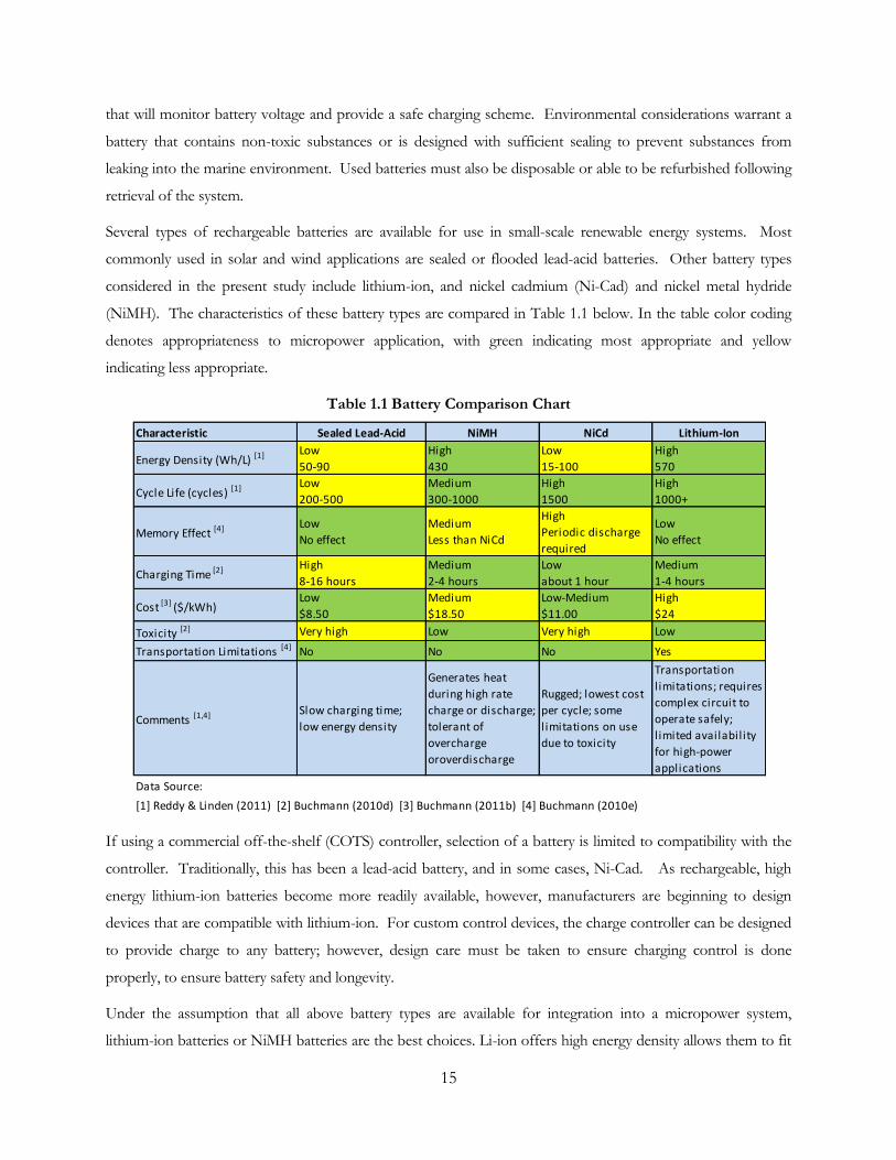
Several types of rechargeable batteries are available for use in small-scale renewable energy systems. Most
commonly used in solar and wind applications are sealed or flooded lead-acid batteries. Other battery types
considered in the present study include lithium-ion, and nickel cadmium (Ni-Cad) and nickel metal hydride
(NiMH). The characteristics of these battery types are compared in Table 1.1 below. In the table color coding
denotes appropriateness to micropower application, with green indicating most appropriate and yellow
indicating less appropriate.
Table 1.1 Battery Comparison Chart
If using a commercial off-the-shelf (COTS) controller, selection of a battery is limited to compatibility with the
controller. Traditionally, this has been a lead-acid battery, and in some cases, Ni-Cad. As rechargeable, high
energy lithium-ion batteries become more readily available, however, manufacturers are beginning to design
devices that are compatible with lithium-ion. For custom control devices, the charge controller can be designed
to provide charge to any battery; however, design care must be taken to ensure charging control is done
properly, to ensure battery safety and longevity.
Under the assumption that all above battery types are available for integration into a micropower system,
lithium-ion batteries or NiMH batteries are the best choices. Li-ion offers high energy density allows them to fit
Characteristic Sealed Lead-Acid NiMH NiCd Lithium-Ion
Energy Density (Wh/L) [1] Low
50-90
High
430
Low
15-100
High
570
Cycle Life (cycles) [1] Low
200-500
Medium
300-1000
High
1500
High
1000+
Memory Effect [4] Low
No effect
Medium
Less than NiCd
High
Periodic discharge
required
Low
No effect
Charging Time [2] High
8-16 hours
Medium
2-4 hours
Low
about 1 hour
Medium
1-4 hours
Cost [3] ($/kWh)Low
$8.50
Medium
$18.50
Low-Medium
$11.00
High
$24
Toxicity [2] Very high Low Very high Low
Transportation Limitations [4] No No No Yes
Comments [1,4] Slow charging time;
low energy density
Generates heat
during high rate
charge or discharge;
tolerant of
overcharge
oroverdischarge
Rugged; lowest cost
per cycle; some
limitations on use
due to toxicity
Transportation
limitations; requires
complex circuit to
operate safely;
l imited availability
for high-power
applications
Data Source:
[1] Reddy & Linden (2011) [2] Buchmann (2010d) [3] Buchmann (2011b) [4] Buchmann (2010e)

16
into a more compact physical space and also has a fairly low charge time. NiMH offers the advantage of being
tolerant to overcharge or over-discharge (Reddy & Linden, 2011). If battery energy storage is dominated by the
semi-diurnal tidal cycle, with two charge and two discharge cycles per day, the battery life of both would be able
to last for a six-month deployment of 365 cycles. The charging time is Li-ion is low to allow for charging during
a cycle peak, and the low memory effect will allow the Li-ion batteries to operate in any state of charge without
maintenance as the tidal cycle fluctuates.
The difficulty with integration of lithium-ion batteries has traditionally been their complex charging
requirements to maintain safety. Additionally, until about the 2000’s the cost of a lithium ion battery was
prohibitively expensive for many applications (Buchmann, 2010b). Their use was initially limited to low power
applications of consumer electronics in well-controlled charging applications. As the batteries gain more
widespread usage, however, they become more versatile. Lithium-ion battery technology is changing rapidly.
Another possibility not explored here is a hybrid two-stage battery system, where a battery of one type is used to
charge a second battery bank.
1.6.5 Controller/Converter
A controller for a micropower system performs several functions related to safety, longevity, and efficiency of
the system. The controller can function in one or more of several modes. As a charge controller, the function
is to prevent battery overcharging and undercharging and to regulate the rate of charge of the batteries. As a
system controller, the device maintains the system at a maximum efficiency operating point. When used as a
load controller, the device would provide current limiting, load regulation and short circuit protection of both
the batteries and the loads. When providing diversion control, the controller switches the system to provide
power to an auxiliary or dump load to prevent overcharging of the batteries. A single, integrated unit may
provide many of these functions. Charge control and system control functions are frequently integrated into a
power converter. The power converter can provide a rectification function, changing an AC generator output to
DC output. For DC generators the converter will control the voltage, changing the generator variable voltage
output to a charging voltage that is compatible with the battery type.
One of the critical functions of a charge controller is to ensure that battery voltage range requirements are met.
Overcharging batteries without a protection circuit may lead, for example, to grid corrosion, gassing, and
rupture in lead-acid batteries or to rupture and venting with flame in lithium-ion batteries. Lithium-ion batteries,
however, often come with a built-in protection circuit (known as a current interrupt device, or CID) that
prevents unsafe overcharge, but overcharging to this point stresses the battery and reduces longevity
(Buchmann, 2010c; Buchmann, 2011a). Dropping the battery voltage too low may cause sulfation in lead-acid
batteries, reducing their performance, or “sleeping” mode for protected lithium-ion batteries, making them
unusable. In system control, to prevent battery over-charge or over-discharge, if the battery voltage reaches the

17
limits of the allowable range, system loads could be shutdown, or the battery circuit opened to prevent damage.
Also, the generated power can be sent to a diversion load to prevent additional charging.
Other optional functions can be implemented at a greater cost and complexity. Multistage charging is used for
conventional lead-acid or Ni-Cad batteries to charge the battery in different modes depending on voltage and
charge state, in order to maximize charging efficiency and battery life. Multistage charging often includes bulk
charge at a constant current or constant voltage high rate, followed by a timed pulsed or tapered charge, and
then a trickle charge once battery voltage is topped off (Reddy & Linden, 2011). Multistage charging is regulated
either by voltage or by timing once a charge cycle is initiated.
Maximum Power Point Tracking (MPPT) is an optional system feedback control method that attempts to keep
the micropower system in an operating state of maximum efficiency relative to the marine current or system
loads. Turbine maximum power output is maintained by adjusting battery voltage or circuit load. An MPPT
algorithm has been designed by the Memorial University of Newfoundland for use in a DC-DC power
converter in a micropower tidal system (Khan, 2008).
No commercial controllers/converters are known to exist for tidal micropower systems. Wind and solar power
charge controllers are readily available and are sold in various stages of complexity, with the most simple design
regulating voltage and providing diversion for a dump load, and the more complex designs used for grid
integration with MPPT tracking and multi-stage charging. A commercial charger compatible with lithium-ion
batteries is, at present, not readily available.
1.6.6 Loads
The loads for an oceanographic instrumentation system with tidal micropower may consist of any number of
devices requiring a low level of continuous or intermittent power. A specific set of instruments is proposed in
the present study in order to define power requirements for the prototype system.
The hypothetical loads to be powered by the micropower system, including their steady state power
requirements, are shown in Table 1.2. These include existing oceanographic instrumentation presently deployed
onto a Sea Spider for site characterization. Also included is instrumentation consisting of a processor, a data
storage device and micropower system charge controller, devices which are feasible only with expansion from a
battery bank energy storage system to a tidal micropower system.

18
Table 1.2 Micropower System Loads
The embedded CPU and solid state storage devices above represent power requirements for specific parts, but
for embedded computing and data storage systems, there are a wide range of units sold on the market that offer
differing levels of capability and power consumption. The parts and capabilities of these units are constantly
improving and changing. Furthermore, the load which would be desired for a system could vary greatly
depending upon mission requirements. Therefore, no attempt is made to define a standard load that must be
used in a micropower system, and the above values only show the level of functionality that was desired when
the power requirement of 20 Watts was developed.
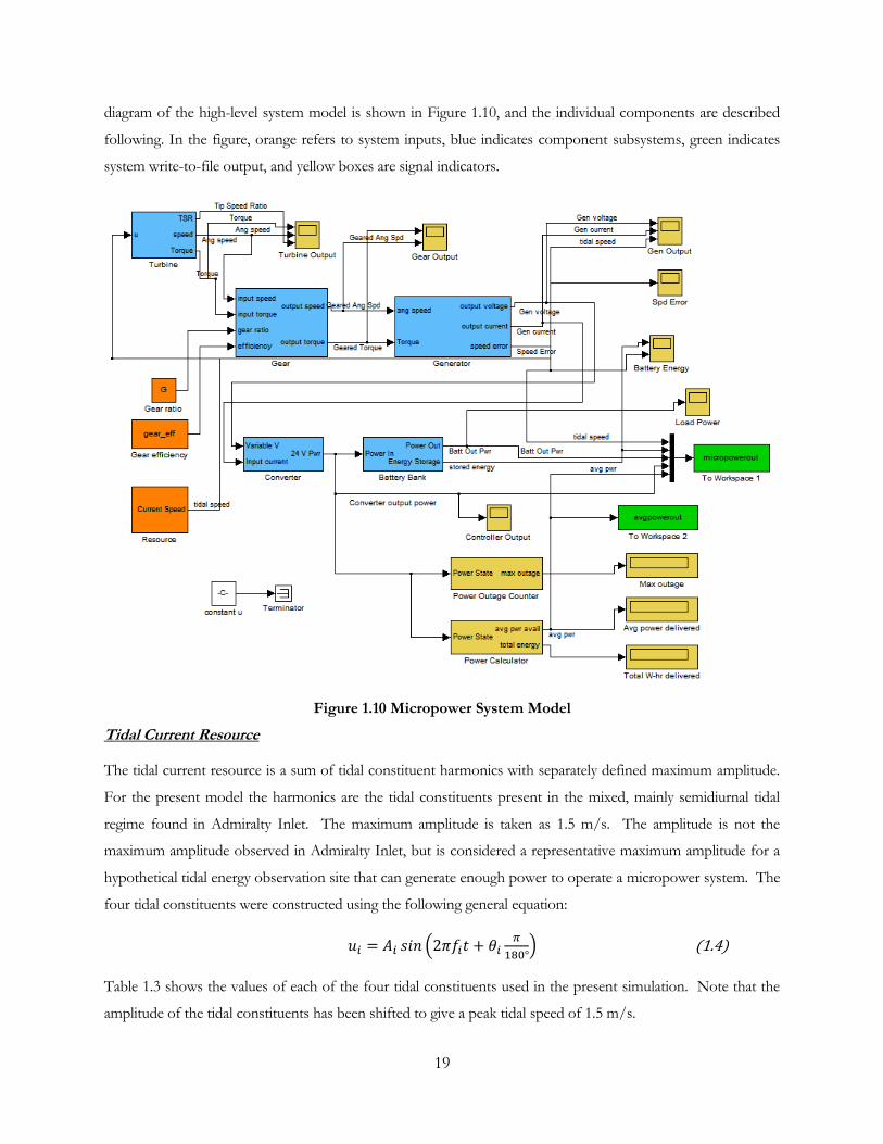
1.7 System Performance Model
A quasi-steady system performance model was developed using MATLAB Simulink to determine the power
output of a micropower system for a given tidal signature. The system calculates the steady output of the
system only and does not account for transient dynamics. The model simulates a tidal current, then converts the
current into an electrical energy, manipulating it using simulated system components. The output is a list of
parameters including power delivered and battery energy storage in W-hr. The model pre-calculates a table of
operating points by finding the intersection point of the turbine torque-rpm curve with the generator torque-
rpm curve, taking into account a gearbox gear ratio, gearbox efficiency, and downstream load resistance. A
Unit Power Usage (W)
Embedded CPU [1]
13.3
Solid State Storage Device[2]
2.6
Charge Controller [3]
1.9
ADCP Monitor [4]
2.2
Hydrophone [5]
0.5
CPOD/TPOD [6]
0.1
Total 20.60
[6] 10 a lka l ine D-cel ls required for 5-6 month deployment.
10 cel ls*31.5 Whr/cel l*(1/6 months)*(1 month/30 days)*(1 day/24 hr)=0.073 W
Source: (Tregenza & Chelonia Ltd, 2011)
[1] For PC/104 standard compatible with SSD. 13.3-14.3 W is used.
Source: (RTD Embedded Technologies Inc, 2011)
[2] 2.6 W for seria l SSD Flash Drive mounted to PC/104 format hard drive
Source: (RTD Embedded Technologies Inc, 2010)
[3] Estimated from charging inefficiency for a s imple control ler at 25 A
Source: (SES Flexcharge USA, 2002)
[4] Source: (RD Instruments , 2001)
[5] Two 9-V cel ls required for 20 hrs l i fe. 2 cel ls*5.49 Whr/cel l*(1/20 hr)=0.458 W
Source: (Cetacean Research Technologies , 2011)
19
diagram of the high-level system model is shown in Figure 1.10, and the individual components are described
following. In the figure, orange refers to system inputs, blue indicates component subsystems, green indicates
system write-to-file output, and yellow boxes are signal indicators.
Figure 1.10 Micropower System Model
Tidal Current Resource
The tidal current resource is a sum of tidal constituent harmonics with separately defined maximum amplitude.
For the present model the harmonics are the tidal constituents present in the mixed, mainly semidiurnal tidal
regime found in Admiralty Inlet. The maximum amplitude is taken as 1.5 m/s. The amplitude is not the
maximum amplitude observed in Admiralty Inlet, but is considered a representative maximum amplitude for a
hypothetical tidal energy observation site that can generate enough power to operate a micropower system. The
four tidal constituents were constructed using the following general equation:
(1.4)
Table 1.3 shows the values of each of the four tidal constituents used in the present simulation. Note that the
amplitude of the tidal constituents has been shifted to give a peak tidal speed of 1.5 m/s.

20
Table 1.3 Tidal Constituent Parameters
Tidal Constituent Ai *(2.9221/1.5) fi θi
M2 1.7 0.0805114 0
S2 0.5 0.0833333 10
K1 0.5 0.0417807 20
O1 0.3 0.0387307 30
Turbine
The turbine is modeled as a torque-rpm performance curve, which is derived from a curve of non-dimensional
parameters: torque coefficient and tip speed ratio (described in Section 2).
In this simulation, the turbine corresponds to a four-bladed helical turbine with 30% solidity, taken from a
modified form of the model extrapolated curve to 1.5 m/s (see Section5.4.3). Figure 1.11 shows torque-rpm
curves for the simulated turbine at different tidal current peak velocities, with the turbine values modified by the
gear ratio (see “Gearbox” below). The turbine dimensions used for the simulation were radius of 0.35 m and
height of 1.0 m.
Figure 1.11 Turbine-Generator Operating Curves
Gearbox
The gearbox provides the transition from the turbine output torque and rpm to the generator input torque and
rpm by stepping up the rpm and stepping down the torque by the gear ratio. The gearbox is modeled as a
simple gear ratio factor, with an efficiency of 97% per stage. The output torque (going into the generator as an
input) is reduced by the gearbox efficiency. The maximum gear ratio per stage is taken as 5:1. For the present
system simulation, the optimum gear ratio for power conversion was 8:1, resulting in a two-stage gearbox with
21
94.1% efficiency. Figure 1.11 shows the turbine-generator operating curves with an 8:1 gear ratio stage acting
between the two components.
Generator
The mechanical side of the generator is modeled as a torque-rpm curve. The electrical side has a voltage-current
curve that corresponds to the mechanical power reduced by generator efficiency. The specific system curve is
defined by the load resistance. The generator simulated was the Windblue Power DC-540, a permanent magnet
synchronous generator with rectified, variable voltage DC output used for wind power applications. The DC-
540 was used based on the availability of the system torque-rpm and voltage-current data provided by the
company. Its high rpm rating requires a high gear stage to effectively transmit power from a tidal turbine.
Figure 1.11 shows the Windblue Power DC-540 torque-rpm curve with a load resistance of 10.5 ohms. As the
load changes, the generator operating curve will change also, but only one curve is shown for simplicity. Where
the generator and turbine operating curves intersect for a given inflow velocity defines the system operating
point.
Converter
The charge controller in the present study is modeled as a voltage converter. Most of the power will be
transferred out of the converter, the only loss due to power consumption by the converter and any component
inefficiency. The voltage conversion is difficult to model without knowing the specifics of the charging
schedule or switching. For the present simulation, no specific converter model was chosen. The unit is
modeled as a typical charge controller efficiency curve (SES Flexcharge USA, 2002). The efficiency is an inverse
function with current, with maximum efficiency of ~96% that is linearly decreasing as current is increased
beyond 5 amps, per Equation (1.5):
. (1.5)
Here I is electrical current and is the unit step function. The efficiency is limited to values of [0,1] in the
model. Additional complexity of the charge controller model may be added upon selection of a specific product
in future work.
Battery Bank
The battery bank is modeled as a simple energy storage integrator based on the system power input and
continuous load power draw. Battery operation is highly dependent on several factors, including battery type,
temperature, charging and discharging characteristics, and battery age. Constructing a highly accurate model
depends on the specific product chosen, the loading, and the environmental characteristics of the surrounding
environment. A simplified lithium-ion battery model is used in the present simulation to represent general
battery charging characteristics. In this model batteries have an initial charge of 90%, energy storage does not
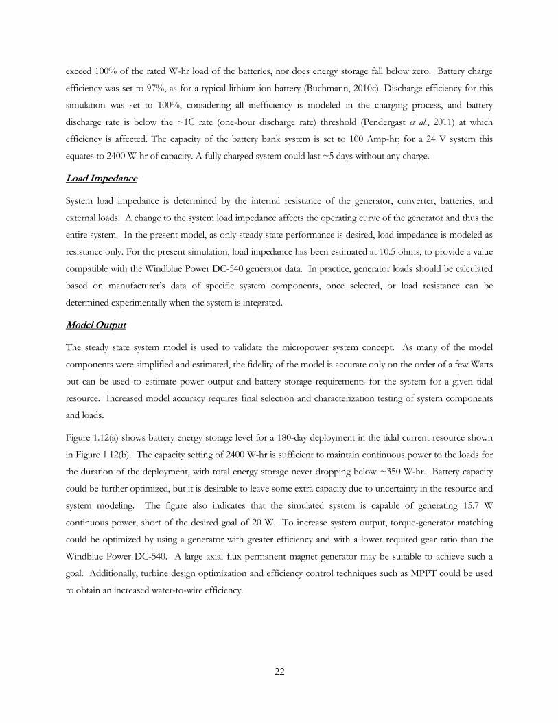
22
exceed 100% of the rated W-hr load of the batteries, nor does energy storage fall below zero. Battery charge
efficiency was set to 97%, as for a typical lithium-ion battery (Buchmann, 2010c). Discharge efficiency for this
simulation was set to 100%, considering all inefficiency is modeled in the charging process, and battery
discharge rate is below the ~1C rate (one-hour discharge rate) threshold (Pendergast et al., 2011) at which
efficiency is affected. The capacity of the battery bank system is set to 100 Amp-hr; for a 24 V system this
equates to 2400 W-hr of capacity. A fully charged system could last ~5 days without any charge.
Load Impedance
System load impedance is determined by the internal resistance of the generator, converter, batteries, and
external loads. A change to the system load impedance affects the operating curve of the generator and thus the
entire system. In the present model, as only steady state performance is desired, load impedance is modeled as
resistance only. For the present simulation, load impedance has been estimated at 10.5 ohms, to provide a value
compatible with the Windblue Power DC-540 generator data. In practice, generator loads should be calculated
based on manufacturer’s data of specific system components, once selected, or load resistance can be
determined experimentally when the system is integrated.
Model Output
The steady state system model is used to validate the micropower system concept. As many of the model
components were simplified and estimated, the fidelity of the model is accurate only on the order of a few Watts
but can be used to estimate power output and battery storage requirements for the system for a given tidal
resource. Increased model accuracy requires final selection and characterization testing of system components
and loads.
Figure 1.12(a) shows battery energy storage level for a 180-day deployment in the tidal current resource shown
in Figure 1.12(b). The capacity setting of 2400 W-hr is sufficient to maintain continuous power to the loads for
the duration of the deployment, with total energy storage never dropping below ~350 W-hr. Battery capacity
could be further optimized, but it is desirable to leave some extra capacity due to uncertainty in the resource and
system modeling. The figure also indicates that the simulated system is capable of generating 15.7 W
continuous power, short of the desired goal of 20 W. To increase system output, torque-generator matching
could be optimized by using a generator with greater efficiency and with a lower required gear ratio than the
Windblue Power DC-540. A large axial flux permanent magnet generator may be suitable to achieve such a
goal. Additionally, turbine design optimization and efficiency control techniques such as MPPT could be used
to obtain an increased water-to-wire efficiency.

23
Figure 1.12 Micropower System Battery Energy Storage
Figure 1.13 shows power delivered to the battery bank as a function of tidal speed. The model simulation
indicates that cut-in speed for the turbine will be about 0.8 m/s, above which the turbine generates sufficient
torque to rotate the generator. As tidal current speed increases above 0.8 m/s, power increases nearly with the
cube of velocity, as would be expected; there is a small deviation from the cube of velocity to account for
change in device efficiency at different operating points. If the system were able to operate below the cut-in
speed of 0.8 m/s, little power would be generated at such low speeds. The conclusion, then, is that care should
be taken to maximize efficiency when tidal current is greatest, for the present study in the range of 1.0 to 1.5
m/s.
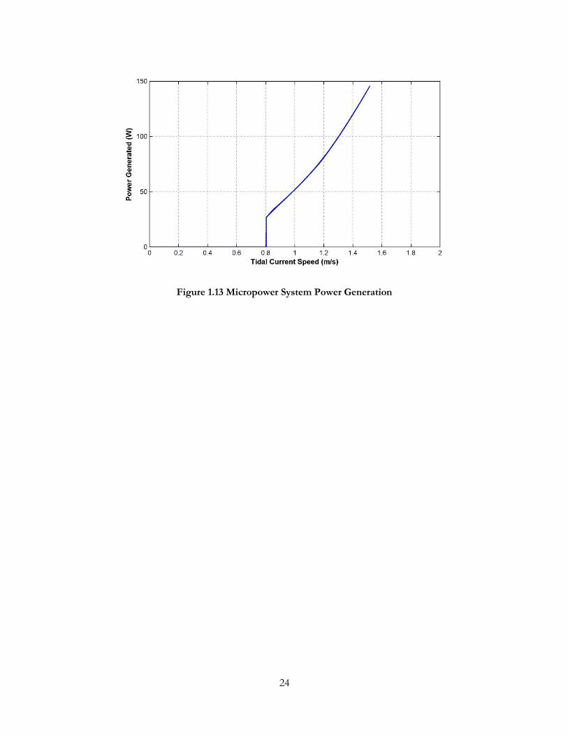
24
Figure 1.13 Micropower System Power Generation

25
2 Turbine Selection
A critical first step in developing a micropower system is design of the hydrokinetic turbine that will extract
energy from the tidal currents. This section focuses on the different turbine types that were reviewed in
selecting a turbine design and describes the parameters that affect their performance.
2.1 Turbine Performance Parameters
Wind and hydrokinetic turbines are usually characterized by a well-known set of non-dimensional performance
parameters. The rotational speed of the turbine is described by the tip speed ratio ( ) which represents the rate
of rotation of the turbine blade at the blade tip relative to the speed of the freestream velocity ( ):
, (2.1)
where is the angular speed of the turbine and R is the turbine radius. The power performance coefficient
( ), or efficiency, of a turbine is represented as the ratio of the shaft power output to the kinetic power
incident on a cross-sectional area the same size as the turbine:
, (2.2)
where is the turbine torque, is fluid density, and is turbine cross-sectional area. The torque coefficient is
similarly defined as ratio of the torque generated by the device to the torque generated by the freestream fluid if
all of the kinetic force could be concentrated at the full radius:
. (2.3)
A static torque coefficient , is calculated for a static turbine by substituting rotating torque in Equation
(2.3) with static torque .
Additionally, various non-dimensionalized Reynolds numbers are defined to describe ratio of inertial to viscous
forces in the flow regime of a turbine. The machine Reynolds number defines the flow regime on a device
scale, while the blade Reynolds number defines the local flow regime at the blade scale:
, (2.4)
and
, (2.5)
where D is the turbine diameter, c is the blade chord length, is the kinematic viscosity of the fluid, and is
the local relative fluid velocity at the blade.

26
2.2 Turbine Types
Hydrokinetic turbines may be classified into two types based on their primary method of converting the force of
the fluid into rotational force.
Drag vs. Lift Devices
One style of turbine is the drag style device. Savonius rotors and cup anemometers are examples drag style
devices (Twidell & Weir, 2006). In drag style devices the primary motive force is the stagnation pressure of the
fluid pushing against the profile of the turbine cup, paddle, or blade (Alam & Iqbal, 2009). The cups are
attached to a central rotating shaft or a conveyor-style attachment. The cups are normally designed such that the
force of the fluid against the retreating cup is greater than the force of fluid against the advancing cup. The
differential force acting at a radius causes torque and rotation.
The second type of turbine is a lift style device. Most axial flow turbines with the classical windmill shape are lift
devices. Cross-flow turbines such as Darrieus and helical turbines are also lift devices. Turbines of this type
make use of lift force developed by fluid motion around an airfoil at an angle relative to the blade chord (known
as the angle of attack) causing a pressure difference on one side of the blade as compared to the other. The lift
force acts perpendicularly to the angle of relative fluid velocity. A drag force is also developed by the fluid
acting on the airfoil, which normally impedes rotation, but for lift devices the average tangential force developed
by lift overcomes the retarding drag force, and the net tangential force acting at a radius on the turbine blade
generates positive torque and power. Figure 2.1 shows the fluid velocity vectors and lift ( ), drag ( ),
tangential ( ) and normal force ( ) vectors acting on a airfoil for tip speed ratio of 1.5.

27
Figure 2.1 Velocity and Force Vectors for an Airfoil
In this diagram is the stream-wise velocity component at the blade (generally a fraction of the freestream
velocity ), is the induced velocity from the turbine rotation, is the relative velocity resultant vector,
and is the relative velocity angle of attack with respect to the chord line.
Generally, drag style devices are easier to manufacture, as they often have simple bowl, flat plate, or cylindrical
shapes, compared to lift style devices that usually incorporate an airfoil shape and are more complex. Drag
devices operate normally at a tip speed ratio below unity, as they cannot rotate faster than the free stream (Alam
& Iqbal, 2009). This also makes the devices theoretically less efficient based on the constraints of the Glauert
criterion (Twidell & Weir, 2006). The slow rotational speed of drag devices makes them more difficult to
integrate with a generator without a high ratio gearbox to step up the rotational speed. A lift device, on the
other hand, normally operates at tip speed ratios above unity, making it easier to integrate with a lower gear
ratio.
Axial Flow Turbines
Another classification of turbines types is by orientation of the flow relative to the rotational axis. Axial flow
turbines, such as the classical windmill rotor shown in Figure 2.2, has the axis and hub of the turbine in the same
direction as the freestream flow. These are the most common types of devices used for large-scale commercial
wind and proposed commercial marine applications, owing to their high efficiency. Maximum water-to-wire
efficiency for some marine devices is around 50% (Polagye et al., 2011).

28
Figure 2.2 Axial Flow Tidal Turbine
(Source: Polagye et al., 2011)
The conventional axial flow windmill turbine design is not ideal for a micropower application. One reason is
that the axis of the turbine needs to be aligned with the current to achieve reasonable efficiencies. Tidal currents
change direction with ebb and flood tide on a diurnal or semidiurnal basis and some locations have significant
ebb/flood asymmetry. Also, there currently is no effective method of aligning a Sea Spider during deployment.
Thus, yaw control becomes critical to power extraction with an axial flow turbine. The yaw control mechanism,
either a wind vane or motorized controller, increases design complexity; a motorized control would also
introduce a parasitic power loss. Additionally, the overall balance of the module and reliability of the yaw
rotation mechanism would need to be considered to prevent tipping or undue fatigue stress on the structure.
Cross-Flow Turbines
A cross-flow turbine has its axis of rotation perpendicular to the freestream velocity, as in a Darrieus rotor or
Savonius rotor. Cross-flow turbines tend to exhibit somewhat lower efficiency than axial flow turbines, but are
advantageous to a micropower application for several reasons. First, they can accept and operate with equal
efficiency with a freestream flow from any horizontal direction without yaw control. Secondly, they have a
symmetric design that makes them a more balanced installation. Several cross-flow turbine designs are
described in more detail in the following sections.
2.2.1 Savonius Rotor
The Savonius rotor was invented by Finnish Engineer S.J. Savonius. The Savonius rotor is a primarily a drag-
style device. The rotor generates high torque at low speeds, making it desirable for applications such as water
pumping and low wind speed applications (Morshed, 2010). The design of the conventional Savonius rotor is
simple and cheap to build – two half cylinders are set with their concave sides facing each other and then offset

29
with a small overlap. The drawbacks of a Savonius rotor are that it has low efficiency and that it operates at low
tip speed ratios ( ) which make it difficult to integrate with a generator.
Several individuals have tested the parameters of the Savonius rotor, devised models to optimize performance,
and altered its conventional design to improve performance. A good summary of experimental performance
testing of the Savonius rotor was given by Ushiyama & Nagai (1988). Ushiyama & Nagai tested several
parameters of the device, as noted in Figure 2.3 below, including gap ratio, aspect ratio, number of cylindrical
buckets, number of stages, endplate effects, overlap ratio, and bucket design (noted in the figure are the (a) gap,
(d) bucket diameter, (e) overlap, and (R) rotor radius). The highest efficiency of all configurations tested was
~24% for a two-stage, two-bucket rotor.
(a) (b)
Figure 2.3 Savonius Rotor Two-Stage Bucket and Diagram (Source: (a) Alam & Iqbal (2009) and (b) Menet (2004))
2.2.2 Darrieus Turbines
A common type of cross-flow turbine that generates torque using lift is the Darrieus turbine. The Darrieus
turbine was developed in the 1920’s and patented in 1931 by G. J. Darrieus (Dai et al., 2011). Two common
types of Darrieus turbines include the troposkein blade shape and the straight-bladed Darrieus (also called H-
Darrieus) turbine, both of which were patented by Darrieus (Islam, 2006) and are shown in Figure 2.4.

30
(a) (b)
Figure 2.4 Sketches of Darrieus Turbine Designs (a) Troposkein blade (b) Straight Blade (Source: Islam, 2006)
The Darrieus turbine is characterized by airfoil-shaped blades that rotate around a central axis, with the axis of
rotation perpendicular to the freestream flow direction. As such, the angle of attack on a cross-flow turbine
airfoil blade section is constantly changing, even for a uniform, constant, freestream flow (as compared to the
axial flow turbines that would have a constant angle of attack in constant freestream flow). The angle of attack
on the airfoils reaches much higher levels than for an axial turbine, particularly for lower tip speed ratios, and the
turbines blades often spend a portion of their rotation in stall. The aerodynamic analysis of a Darrieus turbine is
thus quite complex, and principles of dynamic stall and pitch rate effects should be accounted for in most
analyses (see Section 3.5). Figure 2.5 shows a diagram of a cross-flow turbine depicting velocity vectors and
angles of attack (α) at four different positions. Angle of attack for a cross-flow turbine is commonly defined as
positive when the relative velocity is incident on the exterior half of the blade, and negative when it is on the
interior side; this definition will be used throughout the present study.

31
Figure 2.5 Diagram of Cross-Flow Turbine Velocity Vectors
The Darrieus turbine offers the advantage of a higher operating tip speed ratio compared to a drag device such
as a Savonius rotor. This makes it easier to integrate with a generator and a lower gear ratio is possible.
However the conventional Darrieus turbine suffers from self-start problems at lower flow speeds due its
discrete blade angles and low starting torque (Gorlov, 1998). The hydrodynamic force characteristics of a static
turbine are much different than a rotating turbine because there is no induced velocity vector of the static
turbine. The lift and drag forces for a static turbine are based entirely on the velocity vector of the incoming
hydrokinetic resource; consequently, a static turbine will see much higher angles of attack and lower overall
torque. Drag forces may actually be providing a positive torque that aids rotation.
As a result of the discrete blade positions, some azimuthal angles of a Darrieus turbine may experience a very
low or even negative resultant and the turbine will be unable to start. This issue is particularly noticeable in
turbines with low solidity and low number of blades. The self-start issue can be addressed by motoring the
turbine using the generator and electrical power source, but this is undesirable for stand-alone micropower
applications.
Path of Rotation
α uRELωR
uS
ωR
uS
uREL
α=0
α=0
uS ωR
uREL
uS
ωR
uREL
α
θ ω
R
u0 Undisturbed Freestream
Streamwise flow near turbine
Upstream Pass
Downstream Pass

32
Another issue with the Darrieus turbine is torque oscillation (Gorlov, 1998). The torque oscillation problem is
prevalent at low tip speed ratio, but is gradually diminished at higher tip speed ratio (Khan et al., 2010). . As the
blades rotate around the axis of revolution, the amount of torque generated changes due to the airfoil’s
azimuthal position; since there are a few discrete blade positions, the torque output will pulse as the turbine
rotates. The oscillation increases fatigue of the blades (Gorlov, 1998). The electrical power output will also
exhibit an oscillatory behavior when the turbine is loaded (Khan et al., 2010).
Both self-start and torque oscillation in the Darrieus turbine have been addressed in various ways. Two
common methods are manipulating the blade shape to provide better starting torque or higher lift at low
Reynolds number, or using a hydrid turbine configuration (e.g., Savonius/Darrieus hybrid as discussed in
Section 2.2.3.
Despite the self-start and torque oscillation issues, Darrieus turbines are quite commonly used for wind and
marine energy systems, in part due to their high operating speed, but also due to their fairly high efficiencies, as
numerous test results have indicated. Testing of a 2-bladed 17-meter troposkein wind turbine by Sandia
National Labs resulted in a power coefficient of 38% (Worstell, 1978). Darrieus straight-bladed turbines used
for tidal turbine generation have been tested and are documented in several sources (e.g., Khan, 2008; Dai &
Lam, 2009). An example is Shiono et al. (2002), who reported Darrieus turbine efficiencies for a marine turbine
as high as ~33% for 1.2 m/s flow.
2.2.3 Hybrid Turbines
In an attempt to overcome the self-start problem for a Darrieus turbine, some designers have attempted to
combine different turbine types with the Darrieus turbine. A common combination is to combine a large
Darrieus turbine with small Savonius rotor (e.g., Alam & Iqbal (2009), as shown in Figure 1.5) on the same
rotational axis. The intent is to provide improved torque of the turbine during startup by utilizing the Savonius
rotor’s good starting torque and performance at low tip speed ratios below unity. Once the rotor gets to
sufficiently high rotational speed, lift forces generated by the Darrieus turbine blades allow the turbine to spin
up to full operating speed.
One obvious design challenge of a Darrieus-Savonius hybrid design is the different optimum tip speed ratios of
the two devices. While a Savonius rotor generates optimum lift with , a Darrieus turbine optimum tip
speed ratio is much higher than unity (actual optimum depends on blade design, size and solidity). The two
rotors must be appropriately sized so that their optimum tip speed ratios coincide to the same rotational speed.
Otherwise, the turbine may spin up to an angular velocity that exceeds the Savonius rotor peak operating point;
the overall efficiency then decreases since the Savonius rotor becomes a parasitic load on the entire device.

33
Wakui, et al. (2005) built and tested a hybrid Savonius-Darrieus wind turbine rotor that accomplished power
coefficients up to ~22.5%. The Savonius rotor had two stages and was located at two different locations for
testing: both inside and externally to the troposkein Darrieus turbine, with similar results. The hybrid turbine
performed similarly to the Darrieus turbine alone in terms of power coefficient but had improved starting
torque. Alam & Iqbal (2009) designed a built a similar turbine for marine current applications but experimental
results had very low power output.
2.2.4 Helical (Gorlov) Turbine
The helical turbine was invented by Alexander Gorlov (1995) and is also known as the Gorlov turbine. The
helical turbine is similar to a Darrieus straight-bladed style turbine, except the airfoil blade profile is swept in a
helix profile along its span. A diagram of a four-bladed helical turbine is shown in Figure 2.6.
Figure 2.6 Helical (Gorlov) Turbine
One of the advantages of the helical blade is that it improves the self-start of the turbine compared to a Darrieus
turbine (Gorlov, 1998). As the helical blade shape sweeps along the circumference of rotation of the turbine,
some portion of the blade profile is located at the optimum angle of attack even in static or slowly rotating
conditions, which allows for a more uniform starting torque that less dependent upon turbine azimuthal
position.
Also owing to the helical blade shape is reduction of torque oscillation during rotation (Gorlov, 1998). A
Darrieus turbine tends to experience torque oscillation resulting from the circumferential void space between
the discrete blade positions. A helical turbine with a full blade wrap around its circumference does not
experience this problem; the uniform blade coverage, neglecting end effects and wake dynamics, ideally give the
turbine fully uniform torque, although in reality some variation is likely to occur.

34
Solidity ratio is a turbine parameter introduced here to facilitate further discussion. Solidity ratio refers to the
amount of “solidness” of a turbine. Past researchers have defined solidity ratio in several ways; here it will be
defined as the number of blades multiplied by chord length, non-dimensionalized by the turbine blade
circumferential sweep. This is an intuitive definition of solidity ratio used by Shiono et al. (2002). Equation (2.6)
gives the solidity ratio ( ) for number of blades (B), chord length (c) and turbine diameter (D). This definition
of solidity ratio gives the amount of circumference of the turbine sweep that is solid compared to the total
circumference:
. (2.6)
Gorlov (1998) reported from experimental testing that maximum efficiency for a helical turbine was around
35%. Gorlov’s turbine was three-bladed , 0.61 m diameter, 0.86 m height turbine with NACA 0020 blades and
27% solidity ratio. Gorlov also compared a helical turbine to a Darrieus in terms of performance and found the
helical turbine to be superior. Shiono et al.(2002) reported lower results for a number of different three-bladed
turbines with 0.3 m radius ranging in solidity from 20% to 50% and height of 0.3 to 0.54 m; maximum
efficiency observed by Shiono was 24.4% for a 1.4 m/s flow rate. Shiono also compared the Darrieus turbine
to the helical turbine but found the Darrieus turbine to have higher efficiencies for the same size turbine in the
same flow rate. Experimental tests did, however, verify Gorlov’s claims regarding torque variation: a rate of
pulsation (static torque range divided by average static torque) of ~0.51 was found for a helical turbine
compared to 3.35 for a straight-bladed Darrieus.
2.3 Helical Tidal Turbine Design Parameters
Optimum design of a helical turbine requires an examination of several design parameters, some of which are
consistent with other turbine designs, some of which are unique to the helical shape. This section examines
these design parameters and offers experimental and/or analytical evidence (many derived from Darrieus
turbines) demonstrating the effects of parameter variation. For the helical turbine several of the design
parameters are interdependent. Judicious selection of parameter values will lead to a more efficient design.
2.3.1 Blade Profile
Blade profile shape can have a significant impact on performance due to the pressure forces that develop when
subjected to an incident flow. Some of the blade design parameters include chord length, leading edge profile,
trailing edge profile, blade thickness-to-chord ratio, location of maximum thickness, and blade camber. The
blade chord line connects the leading edge of the blade to the trailing edge of the blade. Blade camber refers to
the position of the mean thickness of a blade along its length. For a symmetric, uncambered blade, the camber
line and the chord line are co-linear. Traditionally, vertical axis turbine blades have been designed with the
common NACA 4-digit series symmetrical profiles (like that of Figure 2.5) due to the availability of the lift and

35
drag data for a large range of Reynolds numbers. However, Islam et al. (2007) provided a parametric analysis for
effect of airfoil shape on straight-bladed vertical axis wind turbine (VAWT) blade profiles and found that
symmetric 4-digit NACA blades performed poorly relative to other blade profiles. For smaller straight-bladed
VAWTs, Islam et al. identified several features desirable for an airfoil profile to obtain optimum performance:
high stall angle, wide range of angle of attack with corresponding low drag, small zero-lift drag coefficient, high
lift-to-drag ratio, high maximum lift coefficient, delayed deep stall, and small roughness sensitivity. An analysis
of experimental and modeling data found the following blade profile attributes to achieve those characteristics:
Cambered blade, with camber facing concave outward, away from the radial direction;
Thick blade profile;
Large leading edge radius;
Sharp trailing edge.
In terms of lift generated, symmetric airfoils (such as NACA 0015 or NACA 0018) generate higher torque than
asymmetric airfoils when the angle of attack is negative (toward the convex side of a cambered airfoil, as shown
in Figure 2.7). Note that for this camber discussion only, sign of angle of attack is defined with respect to the
hydrofoil blade, not with respect to the turbine. Kirke (1998) noted that the majority of power removed from a
vertical axis turbine is on the upstream pass (see Figure 2.5) of the blade compared to the downstream.
Therefore, an airfoil designed to take advantage of lift on the upstream pass (i.e., a cambered-out airfoil) would
have superior overall performance compared to a symmetric airfoil.
Figure 2.7 Angle of Attack Sign Convention on a Cambered Airfoil (Note: Sign convention is different than turbine convention)
Figure 2.8(a)-(e) shows the blade profiles of some asymmetric airfoils noted as superior by Islam et al. (2007),
overlain onto the profile of a NACA 0015 blade, and Figure 2.8 (f) shows the lift-to-drag ratio at =3x10⁵.
Note that these airfoils were evaluated with the objective of generating higher torque at low Reynolds numbers,
particularly at self-start, for a straight-bladed VAWT. For a helical turbine, the self-start problem is inherently
overcome by the helical geometry; therefore, of more concern is overall torque generated per pass at the range
of Reynolds numbers encountered in normal operation. Additionally, a high chord-to-radius ratio (see Section
2.3.2) introduces flow curvature effects and may impact the benefits gained by a cambered airfoil (Islam et al.,
2007). Nevertheless, the increased lift and reduced drag of the asymmetric blade profiles warrants further
investigation when selecting the optimum blade profile for a helical turbine.
Positive α
Negative α
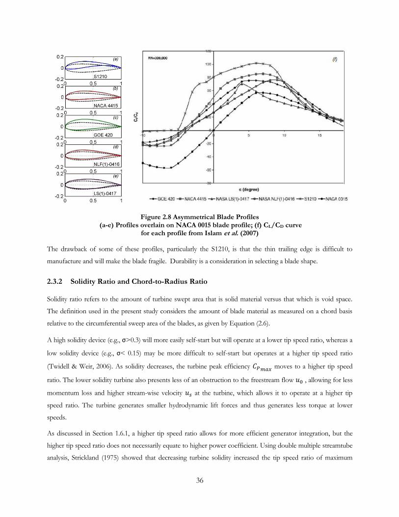
36
Figure 2.8 Asymmetrical Blade Profiles (a-e) Profiles overlain on NACA 0015 blade profile; (f) CL/CD curve
for each profile from Islam et al. (2007)
The drawback of some of these profiles, particularly the S1210, is that the thin trailing edge is difficult to
manufacture and will make the blade fragile. Durability is a consideration in selecting a blade shape.
2.3.2 Solidity Ratio and Chord-to-Radius Ratio
Solidity ratio refers to the amount of turbine swept area that is solid material versus that which is void space.
The definition used in the present study considers the amount of blade material as measured on a chord basis
relative to the circumferential sweep area of the blades, as given by Equation (2.6).
A high solidity device (e.g., σ>0.3) will more easily self-start but will operate at a lower tip speed ratio, whereas a
low solidity device (e.g., σ< 0.15) may be more difficult to self-start but operates at a higher tip speed ratio
(Twidell & Weir, 2006). As solidity decreases, the turbine peak efficiency moves to a higher tip speed
ratio. The lower solidity turbine also presents less of an obstruction to the freestream flow , allowing for less
momentum loss and higher stream-wise velocity at the turbine, which allows it to operate at a higher tip
speed ratio. The turbine generates smaller hydrodynamic lift forces and thus generates less torque at lower
speeds.
As discussed in Section 1.6.1, a higher tip speed ratio allows for more efficient generator integration, but the
higher tip speed ratio does not necessarily equate to higher power coefficient. Using double multiple streamtube
analysis, Strickland (1975) showed that decreasing turbine solidity increased the tip speed ratio of maximum

37
power coefficient, and that for a troposkein Darrieus turbine, the best solidity for obtaining maximum power
was 0.2-0.3. For a helical turbine, the question of optimum solidity ratio for turbine power efficiency has been
addressed by Shiono et al. (2002), who determined the optimum solidity ratio to be 0.3-0.4.
Another concept that is similar to solidity ratio but is useful for examining effects on a per-blade level is chord-
to-radius ratio, which is simply blade chord length normalized by turbine radius:
. (2.7)
The chord-to-radius ratio is useful when comparing turbine secondary effects such as flow curvature effects (see
Section 3.5.3).
2.3.3 Number of blades
The number of blades is directly proportional to solidity. For any turbine, as the number of blades increases, the
chord length of a blade must be decreased to maintain a desired solidity ratio, per Equation (2.6). Conversely,
for constant chord length, the solidity of the overall device will increase as the number of blades increases. If
allowing solidity to increase, increasing number of blades should result in increased starting torque, a lower
operating tip speed ratio and lower overall power performance (Twidell & Weir, 2006). In an experiment testing
with horizontal axis wind turbines, Duquette et al. (2003) found that increasing number of blades while
maintaining solidity constant (i.e., proportionally decreasing the chord length) had mixed results: for flat plate
blades, was relatively unchanged from 3 to 12 blades, but for airfoil-shaped blades, the power coefficient
substantially decreased. This suggests that both number of blades and blade solidity may be responsible for the
shift in power performance. The Duquette et al. results were for axial flow turbines and caution should be
applied in extrapolating the results to cross-flow turbines.
Eventually, as the number of blades is increased, blade wake interference will become an issue, where an
advancing blade’s performance will be impacted by another blade’s wake (Twidell & Weir, 2006). This may
have been the cause of decreased performance in the Duquette et al. experiments. The operating point at which
this begins to impact the design depends on number of blades, size, chord length, and rotational speed.
2.3.4 Aspect Ratio
Aspect ratio (AR) refers to the ratio of turbine height to diameter, as in Equation (2.8) and shown in Figure 2.9.
(2.8)

38
H
D
Figure 2.9 Aspect Ratio
Aspect ratio has also been defined for a Darrieus turbine as ratio of blade length to chord length (Chu et al.,
1985):
, (2.9)
where L is defined as the spanwise length of the blade. Using a double multiple streamtube modeling method
for a Darrieus turbine, Chu et al. determined that coefficient of performance increased with aspect ratio for
blade-length aspect ratio up to a ratio of 12:1. However, starting torque coefficient was inversely
proportional to the aspect ratio.
For a given cross-sectional area (product of H and D), a larger aspect ratio requires longer blade length. As
length increases, mid-span blade support must eventually be considered to reduce deflection, vibration, and
stress on the blades. One must also take into consideration the size constraints for installation and deployment
of the micropower turbine. For the anticipated deployment onto a Sea Spider in a tidal channel, the maximum
turbine height is limited to ~ 1 m for the following reasons:
Ease of deployment from a ship with A-frame winch. The turbine and Sea Spider module must fit
under the winch structure and within its width.
Reduction of overturning moment in high current velocities. The structure must not tip over when
subjected to peak tidal flows.
2.3.5 Helical Pitch Angle
Helical pitch angle ( for a vertical axis turbine refers to the pitch angle that the blade makes with a horizontal
plane. See Figure 2.10 for a depiction of helical pitch angle.
39
δ
Figure 2.10 Helical Pitch Angle
For this analysis, only constant pitch angles are considered, though it is possible for the pitch angle to vary along
the blade length. Shiono et al. (2002) experiments concluded that as helical pitch angle increased, performance of
the turbine improved, up through a 90-degree pitch angle (which is equivalent to a straight-bladed Darrieus
turbine). However, Shiono et al. also showed that static torque variation increased with pitch angle, which is a
known problem for straight-bladed vertical axis turbines at low operating speeds (Reuter & Worstell, 1978).
Shiono et al. compared a 60° and 43.7° degree helix angle by increasing the aspect ratio while holding the
number of blades constant and considering performance normalized by turbine height.
2.3.6 Blade Pitch Angle and Mount Point Ratio
Blade pitch refers to the angle that the airfoil blade chord makes with a line tangent to the circle of revolution of
the turbine. When referenced with respect to the half-chord point, a positive pitch, also referred to as toe-in,
indicates that the blade front half-chord makes an angle toward the center of revolution from the tangent line.
For a negative blade pitch, or toe-out, the blade front half-chord angles away from the center of revolution with
respect to the tangent line. A diagram depicting positive blade pitch is shown in Figure 2.11.
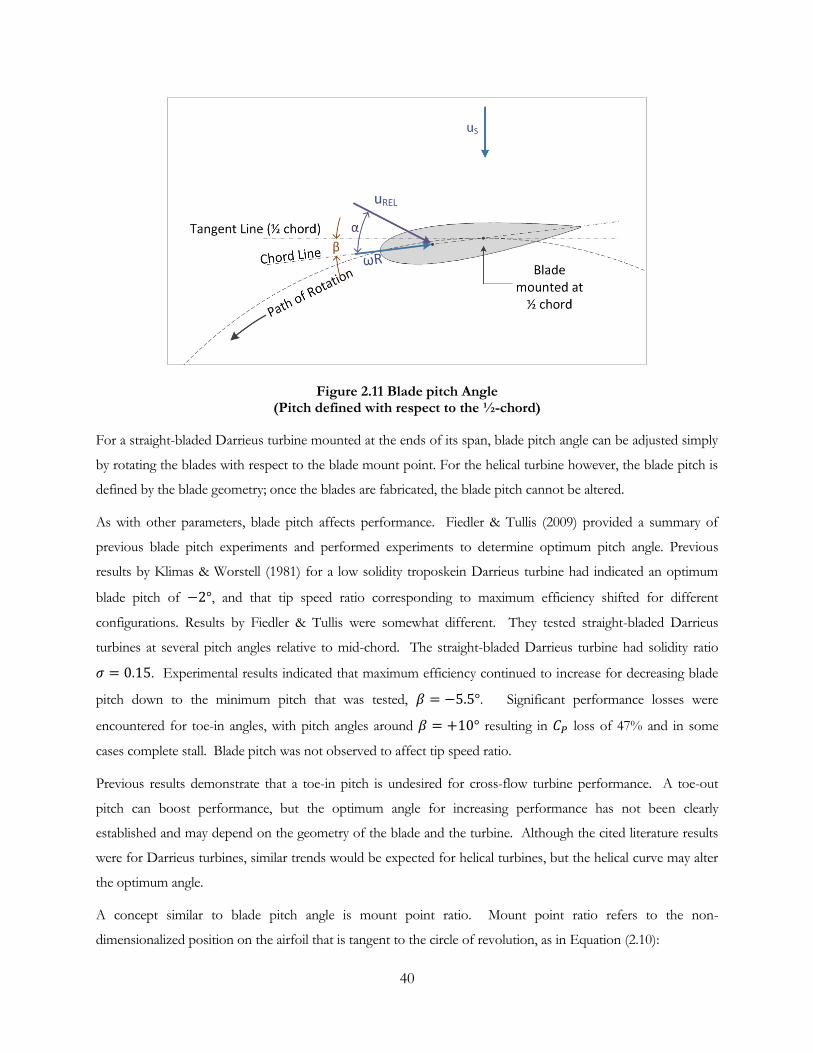
40
Figure 2.11 Blade pitch Angle (Pitch defined with respect to the ½-chord)
For a straight-bladed Darrieus turbine mounted at the ends of its span, blade pitch angle can be adjusted simply
by rotating the blades with respect to the blade mount point. For the helical turbine however, the blade pitch is
defined by the blade geometry; once the blades are fabricated, the blade pitch cannot be altered.
As with other parameters, blade pitch affects performance. Fiedler & Tullis (2009) provided a summary of
previous blade pitch experiments and performed experiments to determine optimum pitch angle. Previous
results by Klimas & Worstell (1981) for a low solidity troposkein Darrieus turbine had indicated an optimum
blade pitch of , and that tip speed ratio corresponding to maximum efficiency shifted for different
configurations. Results by Fiedler & Tullis were somewhat different. They tested straight-bladed Darrieus
turbines at several pitch angles relative to mid-chord. The straight-bladed Darrieus turbine had solidity ratio
. Experimental results indicated that maximum efficiency continued to increase for decreasing blade
pitch down to the minimum pitch that was tested, . Significant performance losses were
encountered for toe-in angles, with pitch angles around resulting in loss of 47% and in some
cases complete stall. Blade pitch was not observed to affect tip speed ratio.
Previous results demonstrate that a toe-in pitch is undesired for cross-flow turbine performance. A toe-out
pitch can boost performance, but the optimum angle for increasing performance has not been clearly
established and may depend on the geometry of the blade and the turbine. Although the cited literature results
were for Darrieus turbines, similar trends would be expected for helical turbines, but the helical curve may alter
the optimum angle.
A concept similar to blade pitch angle is mount point ratio. Mount point ratio refers to the non-
dimensionalized position on the airfoil that is tangent to the circle of revolution, as in Equation (2.10):

41
, (2.10)
where is the mount point ratio, is the mount point distance from the airfoil leading edge, and is
chord length. Traditionally, a blade was assumed to be mounted to the strut or shaft with the mounting point
perpendicular to the shaft radial line; thus the term, “mount point”. Mount point ratio has been used in
traditional vertical axis turbine analysis, such as Strickland et al. (1981a). A depiction of mount point ratio and
how it affects the turbine relative velocity vector is shown in Figure 2.12 and Figure 2.13.
Mount point ratio and blade pitch are fairly interchangeable terms. A blade with mount point ratio equal to 0.50
is very similar to a blade that is mounted at the ¼-chord but has a toed-out blade pitch angle equal to the arc
angle swept by radial lines to the ¼-chord and ½-chord. Since the two points have slightly different radial
distances to the center of turbine rotation, the radius of the turbine would be slightly increased by changing the
discussion from mount point ratio to blade pitch for this example.
Figure 2.12 Blade Mount Point at ¼-chord
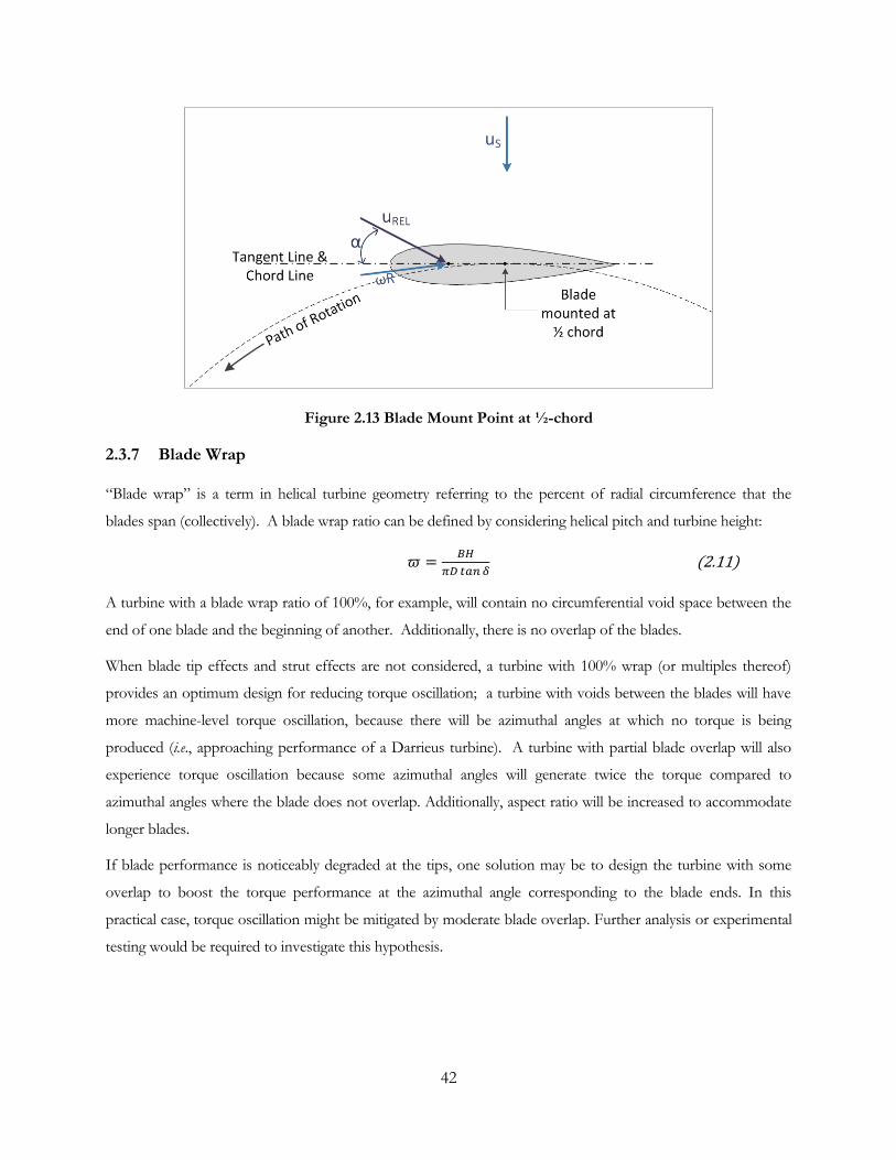
42
Figure 2.13 Blade Mount Point at ½-chord
2.3.7 Blade Wrap
“Blade wrap” is a term in helical turbine geometry referring to the percent of radial circumference that the
blades span (collectively). A blade wrap ratio can be defined by considering helical pitch and turbine height:
(2.11)
A turbine with a blade wrap ratio of 100%, for example, will contain no circumferential void space between the
end of one blade and the beginning of another. Additionally, there is no overlap of the blades.
When blade tip effects and strut effects are not considered, a turbine with 100% wrap (or multiples thereof)
provides an optimum design for reducing torque oscillation; a turbine with voids between the blades will have
more machine-level torque oscillation, because there will be azimuthal angles at which no torque is being
produced (i.e., approaching performance of a Darrieus turbine). A turbine with partial blade overlap will also
experience torque oscillation because some azimuthal angles will generate twice the torque compared to
azimuthal angles where the blade does not overlap. Additionally, aspect ratio will be increased to accommodate
longer blades.
If blade performance is noticeably degraded at the tips, one solution may be to design the turbine with some
overlap to boost the torque performance at the azimuthal angle corresponding to the blade ends. In this
practical case, torque oscillation might be mitigated by moderate blade overlap. Further analysis or experimental
testing would be required to investigate this hypothesis.
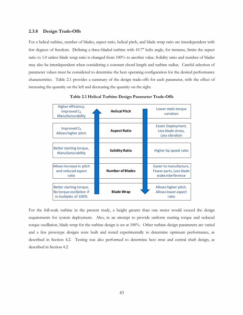
43
2.3.8 Design Trade-Offs
For a helical turbine, number of blades, aspect ratio, helical pitch, and blade wrap ratio are interdependent with
few degrees of freedom. Defining a three-bladed turbine with 43.7° helix angle, for instance, limits the aspect
ratio to 1.0 unless blade wrap ratio is changed from 100% to another value. Solidity ratio and number of blades
may also be interdependent when considering a constant chord length and turbine radius. Careful selection of
parameter values must be considered to determine the best operating configuration for the desired performance
characteristics. Table 2.1 provides a summary of the design trade-offs for each parameter, with the effect of
increasing the quantity on the left and decreasing the quantity on the right.
Table 2.1 Helical Turbine Design Parameter Trade-Offs
For the full-scale turbine in the present study, a height greater than one meter would exceed the design
requirements for system deployment. Also, in an attempt to provide uniform starting torque and reduced
torque oscillation, blade wrap for the turbine design is set at 100%. Other turbine design parameters are varied
and a few prototype designs were built and tested experimentally to determine optimum performance, as
described in Section 4.2. Testing was also performed to determine best strut and central shaft design, as
described in Section 4.2.
Higher efficiency,Improved CP,
ManufacturabilityHelical Pitch
Lower static torque variation
Improved CP, Allows higher pitch
Aspect RatioEasier Deployment,
Less blade stress, Less vibration
Better starting torque, Manufacturability
Solidity Ratio Higher tip speed ratio
Allows increase in pitch and reduced aspect
ratioNumber of Blades
Easier to manufacture,Fewer parts, Less blade
wake interference
Better starting torque,No torque oscillation if in multiples of 100%
Blade WrapAllows higher pitch,Allows lower aspect
ratio

44
2.3.9 Blade Attachment
Blades may be secured at the ends or at one or more mid-span locations, or a combination of both. As the
blade length increases, mid-span struts may be required to reduce vibration, flexure, and stress of the blades.
For smaller turbines and thicker blades, end struts alone may provide sufficient support.
Securing blades using end struts helps to mitigate blade tip effects with increased lift and decreased induced drag
as lift coefficient is increased above 0.2-0.3 of the maximum lift (Reid, 1925). For any attachment scheme,
whether at mid-span or blade end there may be some hydrodynamic performance degradation due to the
interference drag of the strut on the blade.
Blade attachment point can also have an impact on blade pitch, depending on blade attachment method. If the
blade is attached with the chord line not perpendicular to the radial line at the attachment point, a built-in blade
pitch can result, which can positively or negatively impact overall turbine performance. A well-designed vertical
axis turbine should take this built-in pitch into account when designing blade attachment.
2.3.10 Strut Design
Struts provide a stable, rigid connection between the turbine blades and central shaft. However, since the struts
rotate with the blades, drag on the struts reduces the overall efficiency of the machine. Several strut designs
have emerged from previous experimental tests. Some examples follow. The Darrieus turbine developed by
Sandia National Laboratories and tested in the early 1980’s (Sheldahl & Feltz, 1980) had troposkein blades, with
a parabolically- shaped, variable radius (see Figure 2.4(a)). These blades wrapped back toward the central shaft
on each end and connected directly to the central shaft, thus requiring no struts or plates. Lucid Energy’s
spherical turbines adopt a similar approach (www.lucidenergy.com). However, the more common design for
vertical axis marine hydrokinetic turbines is to have a constant blade radius from the central shaft, meaning that
these turbines require a supporting strut to connect the blades to the drive train. New Energy Corporation, Inc.
turbines, as shown in Figure 1.7, use strut arms connected directly to the airfoil blade profile at mid-span (New
Energy Corporation, n.d.). Gorlov’s (1998) helical turbine prototype used thin circular plates at the ends of the
blades to connect the blade to the central shaft. Khan (2008) also used a circular plate with a 6-bladed Darrieus
turbine. Several designs, including the Darrieus and helical turbines built by Shiono et al. (2002), GCK turbines
tested by Verdant Power (2005), and a 3-bladed Darrieus turbine built at the Memorial University of
Newfoundland (Khan 2008) use strut arms at each end of the blade. See Figure 2.14 for an example of the (a)
strut arm configuration and (b) circular plate configuration. The implications for strut geometry are not
discussed in the literature for these tests. For example, Khan (2008) tested several strut types but also
simultaneously varied the blade shape and number of blades, confounding interpretation of the effects of
different struts.

45
(a) (b)
Figure 2.14 Turbine Blade Support Configurations (a) Strut arms (b) Circular plate
Strut drag is a combination of skin friction drag and pressure drag. Skin friction drag is a tangential drag that
develops from the viscous boundary layer friction due to fluid passing over the strut chord. Pressure drag is due
to the profile area whose normal opposes the oncoming fluid velocity. Pressure drag develops from boundary
layer separation due to the strut profile area (Hoerner, 1965).
2.3.11 Central Shaft Design
For devices converting hydrokinetic power to rotational power, a central shaft is required to connect the rotor
to a drive train. A central shaft connecting two turbine support ends aids in aligning the two sides of the turbine.
Additionally, a central shaft allows for the possibility of designing a turbine to be supported from one end,
whereas a shaftless turbine (i.e., a turbine with the two ends plates not connected via a central shaft) is almost
certain to require structural support and bearings on each end to prevent excessive deflection of the blades. The
potential drawback of a turbine central shaft is that shed vortices may degrade the performance of a
downstream blade by reducing hydrodynamic lift. Computational simulations could provide some insight into
these impacts. However, it is likely that the central shaft may already be located in a turbulent flow regime due to
shedding from passing upstream blades; effect of blade wake turbulence will overwhelm any effects due to
vortex shedding from a central shaft.
Central shafts are poorly described in the existing literature. Frequently, shaft diameter and material is not
detailed, even for designs with a central shaft (see Gorlov (1998), Shiono et al. (2002), Verdant Power & GCK
Technologies (2005)). One exception is the three-bladed turbine described by Khan (2008). A shaftless and
cantilevered turbine was tested but performed poorly and was described in the test results as “structurally weak”.
However, as discussed previously, these tests also involved variations in blade geometry, confounding
interpretation of results.

46
3 Vertical Axis Turbine Modeling
Several numerical models have been developed to simulate the performance of cross-flow turbines. Islam et al.
(2008) and Dai et al. (2011) provide excellent summaries of the common modeling techniques, including
development history. This chapter provides a short discussion of blade element theory and momentum models,
followed by a detailed discussion of the vortex model and secondary effects. Other models are detailed in the
appendices.
3.1 Blade Element Analysis
Blade element theory is a method for determining forces on a turbine blade element from the surrounding fluid.
For a rotating turbine, the blade element relative velocity is impacted by not only the incoming freestream
velocity but also the relative rotational velocity acting at the blade tip . Additional velocity components
may also be present if considering the effects of vortex shedding in wakes. Momentarily setting aside vortex
considerations, the vector sum of the rotational and freestream velocities gives rise to a total velocity :
. (3.1)
The relative velocity impinges at an angle relative to the chord line of the airfoil, called the angle of attack ( .
This results in a pressure differential on either side of the airfoil, creating a net lift force. Additionally, the
combination of viscous skin friction drag and pressure drag on the airfoil creates a net drag force on the airfoil.
Although net lift and drag forces on an airfoil may be analyzed numerically (e.g., by XFoil - see Drela, n.d.) by
integrating the pressure distribution over the airfoil, it is common to utilize experimentally derived lift and drag
coefficients from the literature for common airfoils. For most static airfoil data, the lift and drag coefficients are
a function of Reynolds number ( ) and angle of attack ( ).
(3.2)
(3.3)
For tabulated data, the lift and drag forces act at the pressure center of the airfoil, which is assumed to be
located at the “1/4-chord” point located 1/4th of the distance back from the leading edge, corresponding to the
derivation from thin airfoil theory (Anderson, 2001). When considering dynamic effects or the pitching moment
of the blade, other locations are also of importance (Gormont, 1973). For instance, to incorporate pitch rate
effects, the vortex model by Strickland et al. (1979) evaluates lift based on angle of attack at the “3/4-chord” and
drag based on angle of attack at the “1/2-chord” (See Section 3.3 for vortex model).
Figure 3.1 shows a diagram depicting the velocity vectors and the resulting lift and drag forces on a toed-out
pitch turbine blade acting on the quarter chord. The resultant drag force is tangent to the line of relative

47
velocity toward the rear chord line, and the lift force is normal to the relative velocity line on the opposite side
of the airfoil from the angle of incidence.
Figure 3.1 Bladed Element Velocity Vectors, Lift and Drag Forces
Lift and drag coefficients are non-dimensionalized by the product of the dynamic pressure and the blade
element planform area:
(3.4)
and
. (3.5)
In the above equations, and are the lift and drag forces, respectively, and is the blade element
planform area, which is equal to the product of the chord length and blade element span height. Similarly, a
tangential force coefficient (blade leading edge positive) and normal force coefficient (machine inward) can be
calculated:
(3.6)
and
. (3.7)
Taking into account angle of attack and the quarter chord blade pitch (as opposed to half chord blade pitch
defined earlier), the normal and tangential force coefficients and lift and drag force coefficients are related, as
in Equations (3.8) and (3.9).
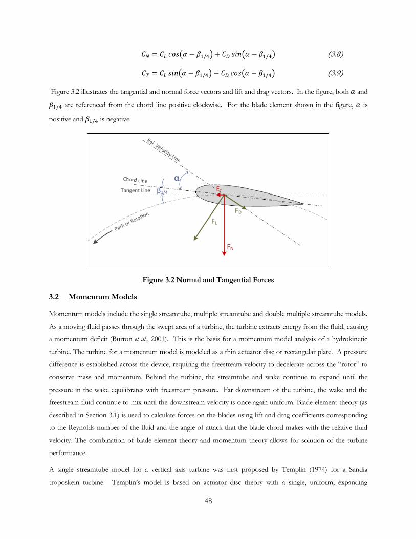
48
(3.8)
(3.9)
Figure 3.2 illustrates the tangential and normal force vectors and lift and drag vectors. In the figure, both and
are referenced from the chord line positive clockwise. For the blade element shown in the figure, is
positive and is negative.
Figure 3.2 Normal and Tangential Forces
3.2 Momentum Models
Momentum models include the single streamtube, multiple streamtube and double multiple streamtube models.
As a moving fluid passes through the swept area of a turbine, the turbine extracts energy from the fluid, causing
a momentum deficit (Burton et al., 2001). This is the basis for a momentum model analysis of a hydrokinetic
turbine. The turbine for a momentum model is modeled as a thin actuator disc or rectangular plate. A pressure
difference is established across the device, requiring the freestream velocity to decelerate across the “rotor” to
conserve mass and momentum. Behind the turbine, the streamtube and wake continue to expand until the
pressure in the wake equilibrates with freestream pressure. Far downstream of the turbine, the wake and the
freestream fluid continue to mix until the downstream velocity is once again uniform. Blade element theory (as
described in Section 3.1) is used to calculate forces on the blades using lift and drag coefficients corresponding
to the Reynolds number of the fluid and the angle of attack that the blade chord makes with the relative fluid
velocity. The combination of blade element theory and momentum theory allows for solution of the turbine
performance.
A single streamtube model for a vertical axis turbine was first proposed by Templin (1974) for a Sandia
troposkein turbine. Templin’s model is based on actuator disc theory with a single, uniform, expanding
49
streamtube accounting for the momentum change across the turbine rotor. Later, a multiple streamtube model
was proposed by Strickland (1975) to improve upon the accuracy of the single streamtube model for vertical
axis turbines, particularly to incorporate wind shear variation and provide a more accurate distribution of blade
forces. Multiple streamtube theory incorporates the same momentum and blade element principles as single
streamtube theory. The major difference is that the single streamtube is divided into several streamtubes that
form a 2-D grid spatially in the plane perpendicular to the stream-wise direction. Double multiple streamtube
theory builds upon multiple streamtube theory by considering that the upstream pass of blades in a vertical axis
turbine reduces the velocity and affects the performance of blades in the downstream pass (Paraschivoiu, 1988).
The analysis is similar to multiple streamtube theory, except that streamtubes are divided into an upstream half-
rotor and downstream-half rotor, with each half being considered separately. Two actuator discs are used to
approximate the turbine, one on the upstream blade pass and the other on the downstream blade pass.
The cascade model, developed by Hirsch & Mandal (1987), is a cross-flow turbine model similar to double
multiple streamtube theory. The model offers an empirical correction for high solidity ratio turbines by
inserting an empirical formula for velocity, and calculating influence of a reference blade on the pressure and
velocity of the other blades.
3.3 Vortex Model
The vortex model was originally developed in two-dimensional form by Fanucci & Walters and by Holme (Dai
et al., 2011). Strickland et al. (1981a) later developed a three-dimensional vortex model that incorporated
dynamic stall effects and was implemented in Sandia National Laboratories VDART3 code. The code still exists
today, with some modifications to include additional dynamic stall effects, pitch rate effects, and strut drag from
supports, and is in use by Sandia for turbine modeling. It is presently given the name CACTUS (Code for Axial
and Cross-flow Turbine Simulation) and is written in FORTRAN F95 language.
In the vortex model, the turbine blade is divided into segments and is represented by a bound vortex. This is
also referred to as a substitution filament or lifting line (Strickland et al., 1979). As the blade segment rotates
around its axis, the bound vortex strength changes and vortices are shed from the blade into the wake at each
time increment. The shed vortex strength is equal to the change in bound vortex strength per Kelvin’s theorem,
which states that over a closed contour the change in circulation over time is zero:
. (3.10)
This can be represented in the model for each blade element i and time t by
. (3.11)

50
In Equation (3.11), is the shed vortex circulation and is the bound vortex circulation. The bound
circulation for the present time is unknown and must be solved. The blade segment also has trailing
vortices which are equal in strength to the bound vortex strength at any given time by the Helmholtz theories of
vorticity, which state that the strength of a vortex ring is constant (Kundu & Cohen, 2008). Considering the
quadrilateral representing the bound, trailing and shed vortices as a closed ring (and that successive rings
overlap), the trailing vortex filament strength can be shown to be equal to the bound vortex filament strength:
. (3.12)
Figure 3.3 illustrates each of the vorticity components for a blade element at successive time increments. The
circulation along the blade length is for the current bound vortex, is the circulation for the vortex at the
previous time increment, etc. The trailing vortices are shown on each end of the blade and are equal to the
current bound vortex, and the shed vortices are shown trailing the blade in the spanwise direction.
Figure 3.3 Vortex Model Blade Element (Adapted from Strickland et al., 1979)
The velocity induced on a point anywhere in the control volume by a vortex filament is found using the Biot-
Savart Law which relates the vortex filament strength to the velocity per Equation (3.13):
. (3.13)
Here is the velocity induced on point P, is the circulation, or strength of any vortex, is the distance
vector from P to a point on the vortex filament, and is the incremental length of a vortex filament, as
illustrated in Figure 3.4. If the distance is zero then the induced velocity is .
Γ1
Γ1
Γ1
Γ2
Γ2
Γ3
Γ3
Γ1-Γ2 Γ2-Γ3 Γ3-Γ4
Shed vortices
Bound vortex
Trailing vortices

51
Figure 3.4 Velocity Induced by a Vortex Filament (Adapted from Strickland et al., 1979)
The laws from vortex theory above are used to predict the velocity induced by all bound, shed, and trailing
vortices on an airfoil, which are added to the freestream velocity and tip-induced velocity components to give a
total relative velocity incident on the airfoil:
(3.14)
Here the subscript i refers to the blade element of interest and j refers to the complete set of wake vortices that
influence blade element i. Equation (3.13) is used to calculate , , . Wall-induced velocities
can also optionally be added to account for effects from a ground plane. The vortex-induced velocity
components are unique to the vortex model as compared to the momentum models that only include reduced
freestream and tip rotational speed components. The inclusion of vortex velocity components allows for better
resolution of the turbine wake velocities and for more accurate average velocity predictions near the blade. In
addition, vortices are represented by a filament line that is initially at the same orientation as the blade element
geometry; this allows for differentiation between a straight-bladed and helical-bladed turbine. The effect of the
vortex-induced velocity components depends on the location of the vortex and the position of the blade. In
general, the vortices contribute to a velocity deficit in the wake of the turbine.
To close the vortex model solution, the bound vortex strength is calculated from the relative velocity and the lift
force according to the Kutta-Joukowski law:
. (3.15)
The lift force is calculated from the lift coefficient using blade element theory as
. (3.16)
uP
dh
Vortex Filament
r
Γ
52
The lift coefficient is found from lookup tables based on the relative velocity and calculated blade Reynolds
number. Combining Equations (3.15) and (3.16), the bound vortex strength is calculated from the lift coefficient
as
. (3.17)
It is important to note that is in the plane of the airfoil. If the bound vortex filament (i.e., the blade
segment) is not orthogonal to , the relative velocity must be resolved into its component in that plane, per
the Independence Principle, which states that a vortex is shed from a yawed obstacle at the yaw angle (Bull &
Dekkers, 1989). For a helical turbine, the angle of the blade segment is the helical pitch angle (see Section
2.3.5); then Equation (3.17) becomes
. (3.18)
(In Equation (3.18), components in the blade spanwise direction are neglected when computing
circulation strength; further refinement may be required if it is found that this component is significant). The
unknowns in the model are the bound vorticity for each element , the lift coefficient and the relative
velocity of each element (in the blade plane), which are solved using Equations (3.2), (3.14), and (3.18).
For each time step and each blade element, the model is iterated numerically until the change in bound vorticity
between successive iterations is within a specified error tolerance. Once the solution converges, force, torque,
and power coefficients are calculated for each blade element at each time step. At each time step, the shed
vortices and trailing vortices are convected downstream at the local relative fluid velocity, a new shed vortex
strength is calculated, and the model loop is repeated for the next time step.
The performance for a single revolution of the turbine is calculated by summing all force, torque and power
coefficients for each element in a time step, then time-averaging the values all times steps in a revolution of the
turbine. Initially, there is no wake developed into the solution, and it is only by successive time iterations that
shed and trailing vortices are generated. Thus, the performance of the turbine in the initial iteration of the
turbine will be different than successive revolution performance. Successive revolutions of the turbine are run
until a full wake has been generated, and the performance coefficients calculated by the model converge to
within a specified tolerance.
The vortex model solution has the advantage over momentum models in that it better resolves velocity and
force components on the blades (Strickland et al., 1979), and it better simulates the turbine wake. Historically,
the approach was considered too computationally intensive to be useful. However, improvements in computing
speed over the past three decades have allowed the solution to converge in a matter of minutes. A vortex
model solution provides a good approximation of turbine performance and wake velocity field (at one rotor
diameter downstream) for a low chord-to-radius ratio turbine (Strickland et al., 1981b). Computational time is
53
completed in a fraction of the time of a Reynolds averaged Navier-Stokes (RANS) or Large Eddy Simulation
(LES) CFD solution. Vortex model correlation for high chord-to-radius ratio turbines, on the other hand, has
been found by subsequent research to provide poor correlation (Dai et al., 2011) for a Darrieus turbine.
3.4 CFD Models
The principal drawback of the streamtube, vortex, and cascade models is that they require lookup tables of static
lift and drag data to calculate the forces on a turbine, even when dynamic effect corrections are implemented.
The static experimental test data is often obtained under ideal, uniform, rectilinear flow conditions. The cross-
flow turbine, on the other hand, operates with the blades in a circular rotation, with constantly varying angle of
attack, and downstream blades are affected by the wake from upstream blades. Furthermore, experimentally
verified tabular data for a particular airfoil profile may not be available. Thus it is advantageous to develop
turbine performance models that organically generate lift and drag characteristics within the model.
Computational Fluid Dynamics (CFD) models offer the advantage over the simpler potential flow models in
that they do not require lift and drag data to resolve the flow structure around a turbine. Additionally, CFD can,
in principle, provide a more accurate representation of ancillary turbine structures including support shafts and
struts (Dai et al., 2011). The main drawback with CFD methods is the computational time and high-power
computing required to resolve the flow structure, even for a two-dimensional simulation. Whereas a double
multiple streamtube solver converges to a solution on the order of seconds, and a traditional vortex model on
the order of minutes, a CFD solution can take a day or more to run a single turbine operating point (Dai et al.,
2011).
CFD models for cross-flow marine current turbines have been recently developed. Ferreira et al (2011)
compared PIV experimental data of dynamic stall for a straight-bladed Darrieus turbine to a 2-D CFD
simulation and found good correlation for a Detached Eddy Simulation model but did not attempt to match
performance predictions to experimental data. Castelli & Benini (2011) provided 3-D CFD simulation results
for a set of helical turbines but did not compare results to any experimental data. Hall (2012) modeled a helical
turbine with the same geometry as a four-bladed prototype turbine in the present study (See Section 4.0) and
found good correlation with experimental data.
Continued work with cross-flow turbine CFD modeling may provide superior performance results relative to
simpler numerical models, but further improvement is needed in this method to improve correlation and reduce
computational time.
3.5 Secondary Effects
When considering small, high solidity cross-flow turbines operating at low tip speed ratios, basic momentum
and vortex models are unable to accurately predict the performance of the turbine. To correct the model
54
predictions, secondary hydrodynamic effects are considered that could appreciably affect turbine performance.
These effects include dynamic stall, pitch rate, and flow curvature effects. Strickland et al. (1981b) incorporated
dynamic stall and pitch rate effects into the vortex model and found well-correlated results. All of these
secondary effects are considered in the present analysis (see Section 5).
3.5.1 Pitch Rate
An unsteady angle of attack leads to variations in static lift and drag coefficients, collectively described as
unsteady hydrodynamics. The lift and drag coefficients for a pitching airfoil are a function of not only the
azimuthal position , relative wind velocity and the angle of attack , but also on the rotation rate of the
turbine , rate of change of rotation rate , the lateral translational heave rate and rate of change of heave
rate (Gormont, 1973). The cross-flow turbine motion is not considered to have heave rates, thus = =0, and
the contribution to lift and drag from the rate of change of rotation , particularly for a smoothly operating
turbine has been determined in previous analyses to be small (Strickland et al., 1981b). According to Strickland et
al. (1981b), and implemented as such in the Sandia vortex model, the pitch rate effects can be approximated by
adjusting the location at which lift and drag are calculated from the ¼-chord position to the following positions:
Lift coefficient CL is calculated from α at the ¾-chord position
Lift coefficient CL is assigned to the ½-chord position
Drag coefficient CD is calculated from α at the ½-chord position and assigned to the ½-chord position.
These approximations were tested for turbines with small chord-to-radius ratio and provided good results.
3.5.2 Dynamic Stall
In a pitching airfoil with sufficient magnitude of angle of attack and rate of change of angle of attack, a vortex
forms at the leading edge of the airfoil and tracks back over the airfoil shape, causing the airfoil to experience a
delayed stall angle and increased lift. As the vortex is finally shed off the airfoil, the airfoil experiences a deeper
stall until the vortex is fully shed and the lift and drag characteristics return to static values (Dai et al., 2011).
This is known as dynamic stall. Diagrams depicting an example of changes to lift and drag of a NACA0012
airfoil due to dynamic stall are shown in Figure 3.5.
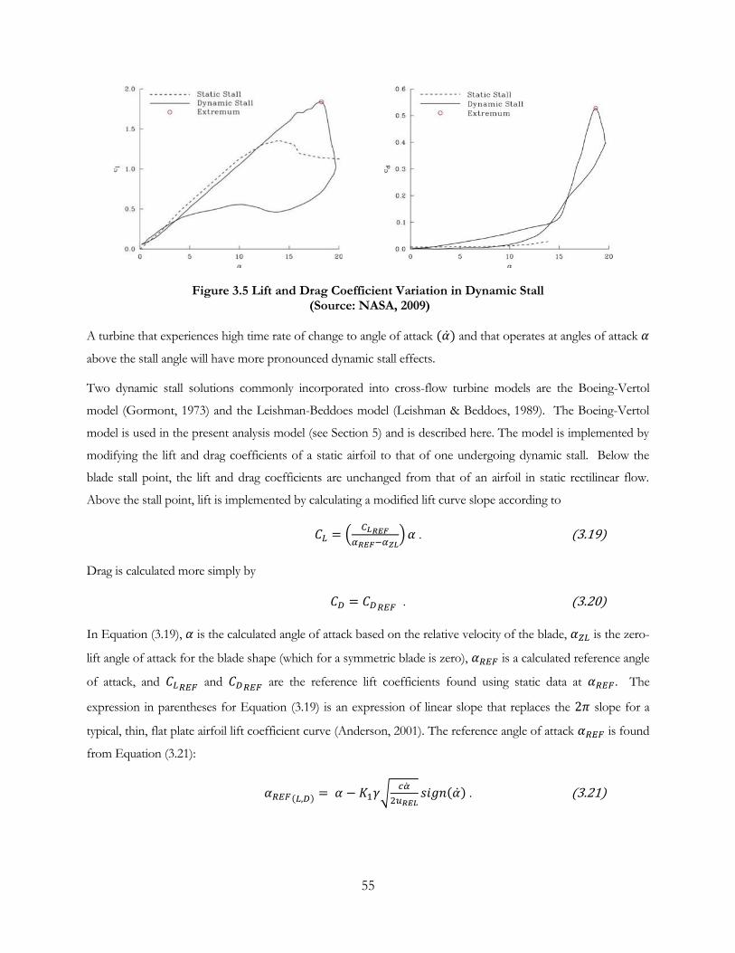
55
Figure 3.5 Lift and Drag Coefficient Variation in Dynamic Stall (Source: NASA, 2009)
A turbine that experiences high time rate of change to angle of attack and that operates at angles of attack
above the stall angle will have more pronounced dynamic stall effects.
Two dynamic stall solutions commonly incorporated into cross-flow turbine models are the Boeing-Vertol
model (Gormont, 1973) and the Leishman-Beddoes model (Leishman & Beddoes, 1989). The Boeing-Vertol
model is used in the present analysis model (see Section 5) and is described here. The model is implemented by
modifying the lift and drag coefficients of a static airfoil to that of one undergoing dynamic stall. Below the
blade stall point, the lift and drag coefficients are unchanged from that of an airfoil in static rectilinear flow.
Above the stall point, lift is implemented by calculating a modified lift curve slope according to
. (3.19)
Drag is calculated more simply by
. (3.20)
In Equation (3.19), is the calculated angle of attack based on the relative velocity of the blade, is the zero-
lift angle of attack for the blade shape (which for a symmetric blade is zero), is a calculated reference angle
of attack, and and are the reference lift coefficients found using static data at . The
expression in parentheses for Equation (3.19) is an expression of linear slope that replaces the slope for a
typical, thin, flat plate airfoil lift coefficient curve (Anderson, 2001). The reference angle of attack is found
from Equation (3.21):
. (3.21)

56
The parameters and are experimentally-determined constants that vary with the sign of and and are
different for lift versus drag coefficients (Gormont, 1973). The reference lift and drag coefficients are found
from static airfoil lift data per
(3.22)
and
. (3.23)
The benefit of the Boeing-Vertol dynamic stall methodology is that it allows the use of static lift and drag airfoil
data to calculate dynamic stall effects. However, Cardona (1984) determined that the method provided results
that sometimes over-predicted lift coefficients and resulted in performance exceeding experimental results.
3.5.3 Flow Curvature
Flow curvature refers to the airflow and performance effects on a cross-flow turbine blade due to variation in
angle of flow impingement (i.e., angle of attack) on the blade along the chord line. For a cross-flow turbine with
a straight blade, the freestream velocity component of the incident airflow impinges upon the airfoil at the same
angle anywhere along the chord. The relative velocity, however, always acts in a direction normal to the turbine
radial line and is therefore impinging upon the airfoil in a constantly changing angle relative to the chord line. In
other words, a straight airfoil in curvilinear motion will have a constantly changing angle of attack along the
chord line. Figure 3.6 illustrates this concept, showing as the angle of attack at the blade leading edge and
as the angle of attack at the blade trailing edge. For high chord-to-radius ratio turbines the angle of attack
variation over a rotation will be large. Traditional static lift and drag data considers the angle of attack only at the
¼-chord position, which can be substantially different from angle of attack at the blade ends and leads to
inaccuracy in the prediction of lift and drag coefficient (Mandal & Burton, 1994).
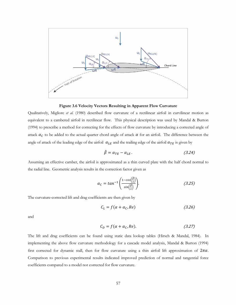
57
Figure 3.6 Velocity Vectors Resulting in Apparent Flow Curvature
Qualitatively, Migliore et al. (1980) described flow curvature of a rectilinear airfoil in curvilinear motion as
equivalent to a cambered airfoil in rectilinear flow. This physical description was used by Mandal & Burton
(1994) to prescribe a method for correcting for the effects of flow curvature by introducing a corrected angle of
attack to be added to the actual quarter chord angle of attack for an airfoil. The difference between the
angle of attack of the leading edge of the airfoil and the trailing edge of the airfoil is given by
. (3.24)
Assuming an effective camber, the airfoil is approximated as a thin curved plate with the half chord normal to
the radial line. Geometric analysis results in the correction factor given as
. (3.25)
The curvature-corrected lift and drag coefficients are then given by
(3.26)
and
. (3.27)
The lift and drag coefficients can be found using static data lookup tables (Hirsch & Mandal, 1984). In
implementing the above flow curvature methodology for a cascade model analysis, Mandal & Burton (1994)
first corrected for dynamic stall, then for flow curvature using a thin airfoil lift approximation of .
Comparison to previous experimental results indicated improved prediction of normal and tangential force
coefficients compared to a model not corrected for flow curvature.

58
3.6 Model Implementation
The above methods describe several theories that can be used for modeling a cross-flow tidal turbine, including
methods for implementing secondary hydrodynamic effects. In the present study, a version of the vortex model
(CACTUS) developed by Sandia National Laboratories is used to model a helical tidal turbine. Dynamic stall,
pitch rate, and flow curvature corrections are implemented into the model. Model results and comparison to
experimental predictions is given in Section 5, following a discussion of experimental results in Section 4.

59
4 Experimental Testing
The following sections describe experimental testing performed with prototype turbines in a flume.
4.1 Test Purpose
The full-scale turbine is intended to be deployed in a tidal channel with velocities up to 1.5 m/s. Scale-models
are deployed in a water flume to inform design decisions for the full-scale installation. Where experimental data
overlaps with prior publications, the data are compared to provide a degree of confirmation to these results.
Measurements of flume velocity and torque, angle, and rotation rate of the experimental turbines allow the
calculation of standard performance characteristics for each design variant. The performance characteristics
mirror those from prior studies (e.g., Shiono et al. (2002)) and include tip speed ratio, power coefficient, torque
coefficient, static torque coefficient, cut-in speed, and cut-out speed. The data are also used to compare with
model predictions presented in Section 5.
The following sections describe the experimental designs, test setup, instrumentation, and tests that are
performed. Test results are presented, and analyses are discussed.
4.2 Experimental Turbine Designs
The full-scale turbine is intended to have a diameter of 70 cm and a cross-sectional area of approximately 0.7
m2. The scale models tested have each have a cross-sectional area of roughly 1/17 scale of that of the full-scale
turbine (i.e., 0.04 m2). The scale-model turbine sizes were chosen to allow them to fit in the Stevenson-Eroglu
water flume (described in Section 4.3) with a low blockage ratio. Three turbine designs were tested in the flume
experiments. Each has the same hydrofoil profile. All are constructed from aluminum alloy. The turbines
differ in the number of blades, helix angle, solidity ratio, and aspect ratio. After some preliminary testing, one of
the turbine designs with a lower solidity was found to perform poorly and its design was abandoned. The other
two were painted prior to formal testing. For the purposes of discussion, these two are referred to as the Four-
Bladed Turbine and Three-Bladed Turbine. The abandoned design was termed the Low Solidity Turbine. The
design parameters for all scale models are shown in Table 4.1.

60
Table 4.1 Turbine Design Parameters
4.2.1 Turbine Design Parameters
Each turbine design parameter is chosen based on results of previous literature or to test the trade-off between
two or more parameters.
Blade profile: NACA 0018 is a common symmetric blade profile that has been frequently in previous
wind and marine turbine design. The turbine’s lift and drag characteristics are well known and
experimental results been published by Sandia National laboratories. NACA 0018 offers a medium
between the improved performance of thinner blades and the durability and manufacturability of a
thicker blade profile. The good self-start capability of the helical turbine reduces the need for a special
cambered blade design to increase self-start.
Blade pitch/Mount Point Ratio: The blade pitch for each turbine is selected so that the blade leading
edge and trailing edge are located at the same radius from the center of rotation, giving each turbine
blade zero pitch and mount point ratio of MP=0.50. At the time of manufacture, it was not known
how this may affect the results. Further experimenting is required to determine the optimum blade
pitch for each turbine design.
Blade Wrap Ratio: Each turbine is given a 100% blade wrap ratio to provide smooth torque and easy
self-start capability.
Parameter
Three-Bladed
Turbine
Four-Bladed
Turbine
Low Solidity
Turbine
Blade Type NACA 0018 NACA 0018 NACA 0018
Blade Material Aluminum Alloy Aluminum 6061-T6 Aluminum Alloy
Blade Finish Green Gloss Paint Blue Gloss Paint Green Gloss Paint
Number of Blades 3 4 3
Radius (m) 0.100 0.086 0.100
Diameter (m) 0.2 0.172 0.2
Blade Height (m) 0.400 0.468 0.200
Aspect Ratio 2.00 2.72 1.00
Blade pitch(degrees at 1/2 chord) 0.0 0.0 0.0
Mount point ratio 0.5 0.5 0.5
Solidity Ratio 0.30 0.30 0.15
Chord-to-Radius Ratio 0.628 0.471 0.314
Chord length (cm) 6.283 4.053 3.142
Chord max width (cm) 1.131 0.729 1.131
Cross Sectional Area (m2) 0.0801 0.0805 0.0400
Helical Pitch Angle (degrees) 43.7 60 43.7
Blade Wrap Ratio (%) 100.0% 100.0% 100.0%

61
Helical Pitch, Number of Blades, and Aspect Ratio: To test this trade-off, the Three-Bladed
Turbine is selected to have a helical pitch that will result in an aspect ratio of AR=1.00 and =43.7°,
and the Four-Bladed Turbine has height increased to accommodate a helical pitch of =60° but with an
additional blade to keep a lower aspect ratio. Literature review did not provide any insight into which
of these designs would be superior, as many parameters are changed at once.
Turbine Height: Each turbine height is selected to provide an aspect ratio that keeps the full-scale
turbine height near the ~1 m limit for installation and deployment concerns.
Turbine Cross-Sectional Area: To provide a consistent basis for comparison, each prototype is
selected to have the same cross sectional area of 0.04 m2. Following selection of turbine height and
cross-sectional area, diameter is determined.
Solidity Ratio: Solidity ratio is selected at σ=0.30 for the Three-Bladed Turbine and Four-Bladed
Turbine, corresponding to the solidity giving best power performance from Shiono et al. (2002) for a
helical turbine. The Low Solidity Turbine is set at half the solidity of the other two designs: σ=0.15, to
determine if the turbine could provide comparable performance at a higher tip speed ratio; the benefit
would be easier integration with a generator. After selection of the diameter and solidity ratio, chord
length for each turbine blade is defined according to Equation (2.6).
Blade Finish: The aluminum blades for the Three-Bladed Turbine and Four-Bladed Turbine are
painted to prevent roughening of the blade surface due to corrosion. The Low Solidity Turbine was
not painted due its poor performance in preliminary testing.
Strut Design: Spoke designs of thickness 2.0 mm and 4.8 mm, and a circular plate design with
thickness 2.0 mm are manufactured to be interchangeable on the Four-Bladed Turbine. The Three-
Bladed Turbine and Low Solidity Turbine have only the original 4.8 mm spoke strut. The focus of the
test is to assess performance of the spoke arm design relative to circular end plates, and to test the
impact of strut profile thickness. Troposkein blade attachment design falls outside the scope of this
work, and strut arms attached at the mid-span requires a more complicated attachment point, but could
be examined in future work.
Central Shaft Design: Central shafts of 6.4 mm and 12.7 mm diameter and corresponding connectors
are made to test central shaft design impact on performance. Additional 6.4 mm shaft stubs are made
to test performance of the turbine with no central shaft between the two turbine ends.
The baseline configuration is defined as the Four-Bladed Turbine with 2.0 mm four-leg spokes and 6.4 mm
central shaft. Other configurations of blade design, strut design, and shaft design are tested and compared to
the performance of the baseline configuration.

62
4.2.2 Manufacturing and Construction
The prototype turbines were manufactured out of aluminum alloy and were cut on a 3-axis CNC mill. The
turbine attachment points and blade alignment were manufactured with precision using a digitized mill and a
female blade jig. Precise alignment of the aluminum struts were made by cutting the design on a water jet with
temporary alignment tabs. Details of the manufacturing process are provided in Appendix A.
4.3 Flume Test Setup and Turbine Installation
Testing was carried out at the Stevenson-Eroglu water flume located in the Guggenheim Building Fluid
Dynamics Laboratory at the University of Washington in Seattle. A user interface allows for selection of the
pump motor electrical frequency, which ultimately controls the pump impeller rotational speed and, therefore,
flume water velocity.
The test section of the flume consists of glass walls for visualization and is 3 meters long and 0.757 m wide. For
testing the turbine, the water depth was varied between 0.46 and 0.5 meters. This increased the water velocity
relative to the maximum operating depth of 0.6 m. A photograph of the test section with turbine test frame
installed is shown in Figure 4.1. The coordinate frame for measuring velocity in each direction is: positive X
stream-wise to the right, positive Y crosswise into the page, and positive Z up.
Figure 4.1 Water Flume Test Channel
The flume’s maximum volumetric flow rate (corresponding to a pump motor electrical frequency of 58 Hz) is
0.25 m3/s and is constant for water depths down to at least 45 cm. Therefore, by decreasing water height, faster
flow velocity can be attained, at the expense of flow stability and higher turbine blockage ratio.

63
During testing it was found that the flume became unstable with static water heights below 46 cm. Waves
began to form downstream of the turbine at the water surface. As the wave troughs reached the flume return
intake, air became ingested due to vortex formation and the low water height, leading to pump instability.
Therefore, to minimize wave formation and instability, the static water height for testing was maintained at or
above 46 cm for a maximum velocity of 0.8 m/s.
The turbine installation is supported by the test frame. The turbine central shaft is supported on both ends by
radial ball bearings. the lower bearing is submerged and is housed on the turbine frame lower cross-bar. The
upper bearing is located in the instrumentation module. The instrumentation module and upper cross-bar, in
addition to the bearings, provide turbine axial support. The test frame is a truss of painted low carbon steel
members; a drawing is shown in Figure 4.2. More details of the frame and installation procedure are provided
in Appendix B.
Figure 4.2 Test Frame, Instrumentation Module, and Turbine
A drawing showing a streamwise view and dimensions is shown in Figure 4.3.

64
Figure 4.3 Test Setup Stream-Wise View (With Four-Bladed Turbine installed)
4.4 Instrumentation
The instrumentation module contains a torque cell, particle brake, optical encoder, and locking plate. The
torque sensor is a Futek TFF425 flange-to-flange reaction torque sensor. The torque sensor is static and
measures torque as the strain between its two flanges, one of which is mounted to a rigid cross-beam on the
frame while the other is connected to the turbine and instrumentation module. An Encoder Products Company
6.7 mm (1/4-inch) through-bore optical encoder is used to measure either turbine angle or rpm. The particle
brake is a Placid Industries B2-12-1 magnetic particle brake with single shaft output and full torque rating of
0.28 Nm. When current is applied to the particle brake via a power supply, magnetic particles within the brake
stator set up a magnetic field that opposes rotation of the brake rotor and generates a braking torque. The
current of the particle brake is proportional braking torque. A rheostat and potentiometer in the circuit of the
particle brake are used to vary current. A circular locking plate with holes at 10-degree increments is attached to
the instrumentation shaft and is used to lock the turbine into a referenced position for static testing. Prior to
testing, a reference point on the turbine was correlated to the locking plate position. A figure depicting the
instrumentation module is shown in Figure 4.4. Output from the torque cell and encoder were sent to a
National Instruments Data Acquisition Module and recording using a program developed using LabVIEW
software.
Water height:47 cm typical
Turbine Height:23.4 cm
Turbine Width: 17.2 cm
Flume Width: 75.7 cm

65
Figure 4.4 Test Instrumentation Module
A Nortex Vector Acoustic Doppler Velocimeter (ADV) measures fluid velocity along three orthogonal axes,
which is referenced to the flume coordinate frame. The ADV uses Doppler shift from acoustic backscatter to
non-instrusively measure velocity at a point in the flow. The data is output at a user-specified reporting rate.
For testing the turbine in the laboratory, all data were sampled at a rate of 4 Hz. The ADV was normally located
in the freestream flow 1 meter upstream of the turbine, except for wake velocity testing (see Section 4.6.5) for
which the ADV was relocated to the desired sampling point of the turbine wake. A photograph of an ADV
module is shown in Figure 4.5.
Figure 4.5 Acoustic Doppler Velocimeter (Source: www.nortekusa.com)
4.5 Test Methodology
Where literature data was unavailable or did not provide conclusive results, experimental tests were conducted
to provide information about the operating characteristics of the turbine. The goal of testing was not to

66
complete a full set of tests for each possible geometry; rather, the purpose of testing was to most efficiently
determine operating characteristics of a turbine configuration and to enable comparison among different
designs.
4.5.1 General Test Procedure
The turbine and frame were placed into the 3-meter water flume channel, 1.7 m (or 9.9 diameters of the Four-
Bladed Turbine) downstream of the flume contraction, with the turbine centerline at the center of flume width
and 23 cm from the flume bottom. This puts the turbine centerline in roughly the center of the flume for a 47
cm dynamic water height. Turbine height in the water column was not varied. The ADV was placed 1.2 m
upstream of the turbine centerline (7.0 diameters), with its focal point centered on the turbine centerline. The
turbine/frame and ADV were placed in these respective locations to give optimal spacing between the flume
contraction, ADV, turbine and flume return ducting, to provide the most uniform, undisturbed flow possible
upstream and downstream of the turbine.
The ADV laptop clock and the Torque cell/encoder laptop clock were synchronized so that flume speed data
could be matched to torque and rotation data. Both ADV and torque cell/encoder data recorded at 4 Hz,
unless otherwise specified in specific test sections. Before each test set the torque cell offset was zeroed with the
turbine installed but with the flume at rest.
The procedure for all steady state tests (all tests except start-up/shutdown tests) was performed as follows:
1) Configure the flume to desired water height. (For most tests the water height was set to 50 cm static
water height to reduce biasing of results by blockage ratio effects)
2) Set pump to electrical frequency to obtain desired flume speed. Allow flume to reach steady state
velocity, as verified by the ADV.
3) Configure turbine to desired state: either statically held in position, rotating at full speed with minimal
loading, or loaded using particle brake. When statically held in position, a pin was inserted into a
reference plate at the desired position to prevent the turbine from rotating. Additionally, the particle
brake was turned on to maximum braking torque in order to reduce vibration amplitude. Alternatively,
when a loaded rotating configuration was required, the particle brake and variable resistors were set to
achieve the desired turbine rpm.
4) Record flume speed data from the ADV, torque data from the torque cell and angular position or
velocity from the optical encoder, as required.
5) Stop recording after 30 seconds or as specified by testing.
67
4.5.2 Specific Test Descriptions
Several different tests were designed to collect turbine data under various operating conditions. Test names and
purpose are listed below.
Load Performance Test
The purpose of this test is to collect torque and rpm data for the range turbine operation starting from
freewheel (no load) and ending at stall. The data are used to compute torque, power, torque coefficient, power
coefficient, tip speed ratio, and freewheel speed for flume velocities from 0.4 to 0.8 m/s. This test defines the
turbine’s basic operating performance curves (i.e., T-rpm, P-rpm, and and curves. The first test
condition recorded torque and rpm at freewheel conditions. For subsequent tests, resistance loading was applied
until desired turbine rpm was reached, in decrements of ~5 rpm for each condition. Plots were labeled with the
average flume speed corresponding to each test set. Measurements at incipient stall are not included in the
results because the turbine was not operating in a steady state condition.
Static Torque Test
This test measures the static torque of a stationary, locked turbine at discrete angles as the turbine is rotated
about its axis of revolution. This test provides an indication of how easily the turbine will start to rotate from a
static position (i.e., cut-in on a quickening tide). Also, variations in static torque with respect to angle help
identify “soft spots” in the turbine torque performance.
Each turbine design was tested at 0.7 m/s flow rate. Preliminary testing demonstrated that this was the
optimum flow speed for generating measurable torque and for keeping torque variation and vibration of the
flume small. Tests were performed for the full revolution of the turbine to determine the difference in
theoretically identical blade orientations. Other tests were performed only along a single blade length to get
comparison of two designs.
The test was set up by fixing the locking plate such that the 0-degree mark on the locking plate corresponded to
the leading edge of a reference blade end (Blade End #1). The 0-degree position of the turbine corresponds to
the lower leading edge of the reference blade end with azimuthal position θ=0 as shown in Figure 2.5. For each
test, the turbine was locked into the desired position by inserting a pin into the corresponding hole in the
locking plate and through a hole in the fixed plate in the instrumentation module. Static torque data and flume
speed data were recorded in increments of 10 degrees.
Data results show average static torque for each angular position θ and non-dimensionalized static torque
coefficient CQS versus angular position. Error bars with standard deviation of data were plotted. Plots are
labeled with the flume speed corresponding to each test set.

68
Start-up/Shutdown Test
The intent of this test is to determine the flow start-up and shutdown characteristics of the turbine. A cut-in
and cut-out speed of the turbine are defined as the stream velocity at which the turbine completes its first full
revolution and at which the turbine initiates its last full revolution, respectively. The cut-in and cut-out speeds
are likely to change based on flume acceleration rate, but are defined to determine relative performance with
different starting angles and initial torque.
For this test, the turbine is set to an initial reference angle with the turbine and flume at rest. The optical
encoder is set to measure turbine angle. The pump is then commanded to a frequency corresponding to a
desired steady state flume speed of 0.7 m/s. Angle and torque of the turbine are measured, and the ADV
records the corresponding flume velocity as the flume speed is accelerated from rest until steady state speed is
reached. The turbine is allowed to operate at steady state for a minimum of 10 seconds, then the pump is
commanded off and the flume and turbine are allowed to come to rest. Data is recorded until the turbine ceases
to rotate. The acceleration rate and deceleration rate of the flume are 0.015 m/s2 and -0.028 m/s2, respectively.
Tilted Turbine Test
Ideally, a full-scale turbine used to power instrumentation would be deployed on a level surface in order to
minimize the overturning moment on the foundation and to orient the turbine such that its axis of rotation is
vertical and the mean tidal flow is perpendicular to the vertical axis. However, the seafloor in high-current areas
tends to be irregular and tilt angles up to 10° from vertical could occur. The intent of this test is to determine the
scale of performance degradation for several angles of tilt.
Three sets of angle blocks were used to raise the downstream end of the turbine test frame to tilt angles of 2.5°,
5°, and 10°. For each inclination angle, and for a 0° inclination angle condition, the turbine was subjected to a
Load Performance Test, where torque, rpm and flume speed were measured for the turbine from freewheel to
stall. The flume speed for this test was set to 0.72 m/s. Prior to testing at each angle, the torque cell was zeroed
to subtract off any static loading bias due to inclination angle. A photograph showing the frame, turbine and
instrumentation at a 10° tilt angle is shown in the photograph of Figure 4.35.

69
Figure 4.6 Test Setup for Tilted Turbine Test
Wake Measurement Test
This test measures the wake velocity along the turbine centerline for a turbine under various loading
configurations:
Minimum loading, near freewheel velocity;
Turbine operating near maximum efficiency;
Turbine stalled to a static state at the 0° reference angle.
The purpose of this test is to provide experimental data describing the wake of the helical turbine and to provide
an experimental comparison for numerical and analytical predictions of mean wake velocity. Velocities both
upstream and downstream of the turbine are recorded at several positions in the stream-wise direction.
To measure the wake velocity, the ADV is placed at various points along the flume channel upstream and
downstream of the turbine, always with the ADV focal point measuring velocity along the turbine centerline.
The flume is configured for 0.78 m/s and the turbine is configured to one of the operating states above. Data is
recorded (measuring velocity in the X, Y and Z coordinate axes) for a minimum of 30 seconds at each location.
For most tests, the turbine was located in its usual position 170 cm downstream of the flume channel entrance.
However, due to the finite length of the flume, to get test data points of the far downstream wake (greater than
100 cm downstream of the turbine), the turbine was relocated 100 cm upstream to the 70 cm location. To
determine any differences in the wake between the two locations, two tests with identical relative X-positions
were taken: 20 cm and 60 cm. Non-dimensionalized mean velocity in stream-wise (X), crosswise (Y), and
spanwise (Z) directions and standard deviation of the data are calculated.
Table 4.2 shows the matrix of test conditions completed. The following sections do not present all data from
each test, but rather data from selected tests that best display performance or provide a comparison.

70
Table 4.2 Test Matrix
A few aspects of turbine performance are not discussed in detail, but are worth noting.
First, the turbine performance was tested in both clockwise and counter-clockwise directions by flipping the
turbine upside down. No significant performance difference was observed.
During preliminary testing and prior to painting of the blades, the Three-Bladed Turbine, was tested, allowed to
sit in the flume for 24 hours, and tested again. Qualitatively, the turbine power output dropped significantly and
rotation speed was much lower after resting in fresh water for 24 hours. The blades had developed minor
corrosion that increased surface roughness. This demonstrated the need for protective coatings and for
removing the turbines from the water between tests to minimize the effect of corrosion.
Similarly, two performance tests were completed for the same turbine configuration on the same day to verify
consistency in test results. This testing was performed on the last day of the test schedule. The first test was
completed at the beginning of the day, and the second performed at the end of the test day, after several hours
of testing. The turbine showed an increase in power efficiency at the end of the day relative to the beginning of
the day (from 19.2% to 20.9% peak efficiency). The lower performance at the beginning of the day is likely due
to the build-up of corrosion on the lower bearing from previous day’s testing. After several hours of testing, the
corrosion on the bearing was worn off, reducing the friction. Because it is located on the bottom of the frame,
the friction on the lower bearing is not measured by the torque cell.
Startup -
Shutdown
Wake
Measure-
ment
0.8 0.7 0.6 0.5 0.4 0-0.7 0.78
Turbine Design Strut Design
Shaft
Diameter
(mm) -- -- -- -- --
Single
blade
length
Full
Revolution --Load Per-
formance
Static
Torque --
Single Blade, from
4-bladed turbineCircular Plates 6.4
X X
4.8 mm, 4-leg
spokes6.4
X X X
No shaftX X X
6.4X X X X X X X X X X
12.7X X X
Circular Plates 6.4X X X X X X X X
3-bladed turbine4.8 mm, 3-leg
spokes6.4
X X X X X
Low Solidity
Turbine
4.8 mm, 3-leg
spokes6.4
X X
X: Test Completed
Flume Velocity (m/s):
Performance test Tilted Turbine
2.0 mm, 4-leg
spokes4-bladed turbine
0.7
Turbine Geometry Static Torque
0.72
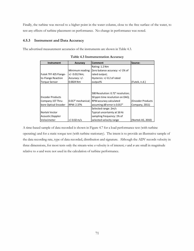
71
Finally, the turbine was moved to a higher point in the water column, close to the free surface of the water, to
test any effects of turbine placement on performance. No change in performance was noted.
4.5.3 Instrument and Data Accuracy
The advertised measurement accuracies of the instruments are shown in Table 4.3.
Table 4.3 Instrumentation Accuracy
A time-based sample of data recorded is shown in Figure 4.7 for a load performance test (with turbine
operating) and for a static torque test (with turbine stationary). The intent is to provide an illustrative sample of
the data recording rate, type of data recorded, distribution and signature. Although the ADV records velocity in
three dimensions, for most tests only the stream-wise u velocity is of interest; v and w are small in magnitude
relative to u and were not used in the calculation of turbine performance.
Instrument Accuracy Comment Source:
Futek TFF 425 Flange-
to-Flange Reaction
Torque Sensor
Minimum reading:
+/- 0.012 Nm;
Accuracy: +/-
0.0024 Nm
Rating: 1.2 Nm
Zero balance accuracy: +/-1% of
rated output;
Hystersis: +/-0.2 of rated
output% (Futek, n.d.)
Encoder Products
Company 15T Thru-
bore Optical Encoder
0.017° mechanical;
RPM: 2.37%
500 Resolution: 0.72° resolution;
50 ppm time resolution on DAQ;
RPM accuracy calculated
assuming Δθ error is 0.017°
(Encoder Products
Company, 2011)
Nortek Vector
Acoustic Doppler
Velocimeter +/-0.02 m/s
Selected range: 2m/s
Typical uncertainty at 16 Hz
sampling frequency: 1% of
selected velocity range (Nortek AS, 2010)

72
Figure 4.7 Instrumentation Output Sample for Performance and Static Tests
The variation in torque measurement for the Static Torque Test is much higher than the variation for a Load
Performance Test with the turbine operating. For the load performance test, the spread for torque as measured
by the torque cell, velocity as measured by the ADV, and rpm as measured by the encoder are less than 3%, for
the static torque test the spread for torque is roughly an order of magnitude higher. It is believed that this is due
to torque pulsations induced by vortex shedding off the turbine blades in the static test (as shown by what
appears to be low frequency periodic fluctuations in the static torque upon careful observation of Figure 4.7(e)).
Qualitatively speaking, the torque cell was highly sensitive to small deviations in the test setup, such as
orientation of the torque cell interface cable and the torque applied to fasten the bolts attaching the torque cell
to the frame and instrumentation module. To maintain consistency in measurements, the torque cell data was
monitored to ensure that its at-rest reading was close to zero (<0.005 Nm output). Prior to beginning a test set
each day, and at other times as necessary, the torque cell was re-zeroed to ensure sufficient accuracy in the data.
ADV data provided a small spread of data, but was prone to quickly becoming erratic (after 10 seconds or so) if
the velocity of the flume was dropped to zero. There was an approximately 10-second lag for the ADV
measurement quality to degrade or improve as velocity was dropped to zero or increased from zero,
respectively. For tests where flume velocity was constant and non-zero, this was a non-issue, as 30 seconds of
steady-state operation were allowed after starting the flume before beginning recording. Only during start-up
Load Performance Test Static Torque Test
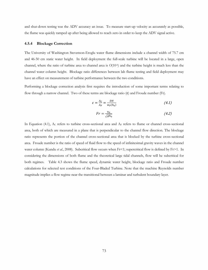
73
and shut-down testing was the ADV accuracy an issue. To measure start-up velocity as accurately as possible,
the flume was quickly ramped up after being allowed to reach zero in order to keep the ADV signal active.
4.5.4 Blockage Correction
The University of Washington Stevenson-Eroglu water flume dimensions include a channel width of 75.7 cm
and 46-50 cm static water height. In field deployment the full-scale turbine will be located in a large, open
channel, where the ratio of turbine area to channel area is O(10-6) and the turbine height is much less than the
channel water column height. Blockage ratio differences between lab flume testing and field deployment may
have an effect on measurement of turbine performance between the two conditions.
Performing a blockage correction analysis first requires the introduction of some important terms relating to
flow through a narrow channel. Two of these terms are blockage ratio ( ) and Froude number (Fr).
(4.1)
(4.2)
In Equation (4.1), AC refers to turbine cross-sectional area and AF refers to flume or channel cross-sectional
area, both of which are measured in a plane that is perpendicular to the channel flow direction. The blockage
ratio represents the portion of the channel cross-sectional area that is blocked by the turbine cross-sectional
area. Froude number is the ratio of speed of fluid flow to the speed of infinitesimal gravity waves in the channel
water column (Kundu et al., 2008). Subcritical flow occurs when Fr<1; supercritical flow is defined by Fr>1. In
considering the dimensions of both flume and the theoretical large tidal channels, flow will be subcritical for
both regimes. Table 4.3 shows the flume speed, dynamic water height, blockage ratio and Froude number
calculations for selected test conditions of the Four-Bladed Turbine. Note that the machine Reynolds number
magnitude implies a flow regime near the transitional between a laminar and turbulent boundary layer.
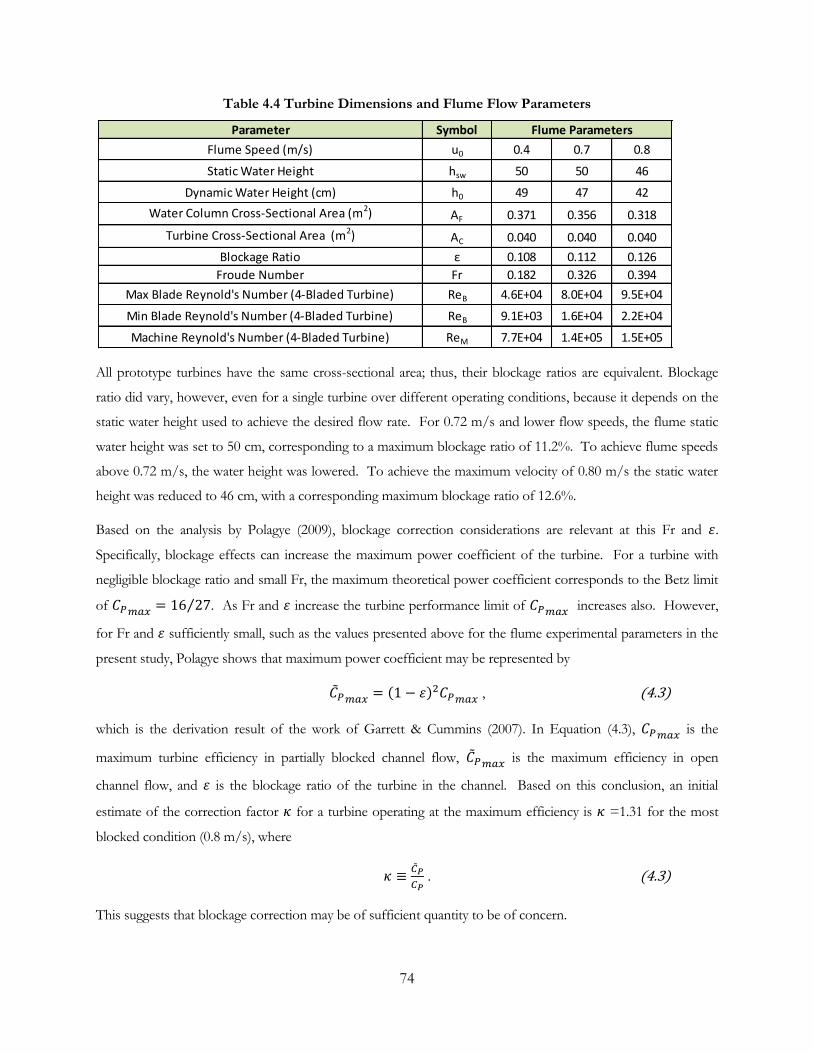
74
Table 4.4 Turbine Dimensions and Flume Flow Parameters
All prototype turbines have the same cross-sectional area; thus, their blockage ratios are equivalent. Blockage
ratio did vary, however, even for a single turbine over different operating conditions, because it depends on the
static water height used to achieve the desired flow rate. For 0.72 m/s and lower flow speeds, the flume static
water height was set to 50 cm, corresponding to a maximum blockage ratio of 11.2%. To achieve flume speeds
above 0.72 m/s, the water height was lowered. To achieve the maximum velocity of 0.80 m/s the static water
height was reduced to 46 cm, with a corresponding maximum blockage ratio of 12.6%.
Based on the analysis by Polagye (2009), blockage correction considerations are relevant at this Fr and .
Specifically, blockage effects can increase the maximum power coefficient of the turbine. For a turbine with
negligible blockage ratio and small Fr, the maximum theoretical power coefficient corresponds to the Betz limit
of . As Fr and increase the turbine performance limit of increases also. However,
for Fr and sufficiently small, such as the values presented above for the flume experimental parameters in the
present study, Polagye shows that maximum power coefficient may be represented by
, (4.3)
which is the derivation result of the work of Garrett & Cummins (2007). In Equation (4.3), is the
maximum turbine efficiency in partially blocked channel flow, is the maximum efficiency in open
channel flow, and is the blockage ratio of the turbine in the channel. Based on this conclusion, an initial
estimate of the correction factor for a turbine operating at the maximum efficiency is =1.31 for the most
blocked condition (0.8 m/s), where
. (4.3)
This suggests that blockage correction may be of sufficient quantity to be of concern.
Parameter Symbol
Flume Speed (m/s) u0 0.4 0.7 0.8
Static Water Height hsw 50 50 46
Dynamic Water Height (cm) h0 49 47 42
Water Column Cross-Sectional Area (m2) AF 0.371 0.356 0.318
Turbine Cross-Sectional Area (m2) AC 0.040 0.040 0.040
Blockage Ratio ε 0.108 0.112 0.126
Froude Number Fr 0.182 0.326 0.394
Max Blade Reynold's Number (4-Bladed Turbine) ReB 4.6E+04 8.0E+04 9.5E+04
Min Blade Reynold's Number (4-Bladed Turbine) ReB 9.1E+03 1.6E+04 2.2E+04
Machine Reynold's Number (4-Bladed Turbine) ReM 7.7E+04 1.4E+05 1.5E+05
Flume Parameters

75
Polagye (2009) showed that power coefficient (and therefore blockage correction factor) is a function of Fr, ,
and wake velocity ratio . Since is unknown, however, no attempt is made in the following sections of data
results to correct for blockage ratio. However, a proposed methodology for providing a more accurate bounding
limit to the increase in power coefficient due to blockage is provided in Appendix D.
4.6 Test Results for Baseline Configuration
The baseline test configuration is the Four-Bladed Turbine with 2.0 mm 4-leg spokes and 6.4 mm central shaft.
In the following sections, test results for the baseline configuration for the Load Performance Test, Static
Torque Test, Tilted Turbine Test, Start-up/Shutdown Test, and Wake Velocity Test are presented. Blade, strut
and shaft design parameters are then varied and compared to the baseline configuration (except for comparison
to the Three-Bladed Turbine, where the thicker 4.8 mm strut is used).
4.6.1 Load Performance Test
Full performance curves over several flume speeds were tested for the baseline configuration. A photograph of
the turbine configuration is shown in Figure 4.8.
Figure 4.8 Baseline Turbine Configuration
Figure 4.9 shows the load performance of the baseline configuration. Maximum power coefficient for this
turbine design occurs in 0.8 m/s flow (for the testable flow rates). The maximum power coefficient was 0.209,
corresponding to a power of 2.2 W, at 142 RPM. As Figure 4.9(d) shows, the turbine maximum efficiency
continued to increase as flume velocity was increased from 0.4 m/s to 0.8 m/s. Additionally, there was a
shift in tip speed ratio at maximum efficiency toward a higher tip speed ratio.
Looking at the lift and drag coefficient tables plotted versus Reynolds number for several angles of attack as
shown in Figure 4.10, it is readily apparent why is increasing with increasing flume velocity. As flume
velocity is ramped up, the effective blade Reynolds number is increasing per Equation (2.5). In the range of
76
velocities tested in the flume experiments, the turbine is operating with blade Reynolds numbers on the order of
104-106 (actual value depends magnitude of relative velocity calculated at the blade). In this transitional Reynolds
number regime, the lift coefficient increase is linear with (although for different angles of attack
the region of linear relationship varies), while the drag coefficient remains fairly flat or decreases. Increased
lift with steady drag results in an increase in turbine performance. However, the magnitude of does not
continue to increase indefinitely for two reasons:
Lift curves slope begin to flatten out with increasing ;
As performance is increased, tip speed ratio increases, resulting in a lower average angle of attack.
Eventually, as inflow velocity is continued to increase, the turbine will reach a state where an increase in flow
velocity does not improve and a stable vs. curve is obtained. The above performance
characteristics can also explain the differences in results by Shiono et al. (2002) and Bachant (2011). Shiono et al.
(2002) found that performance of a turbine increased with increasing flume velocity, whereas Bachant (2011)
found that performance remained steady. The difference lies in the tip speed ratio of the two experiments.
While the blade Reynolds numbers were the same (~4.4x10⁵ for Shiono et al. versus ~4.5x10⁵ for Bachant),
Shiono was operating at a lower tip speed ratio (~1.5) than Bachant (~2.3), resulting in a much average lower
angle of attack for the turbines tested by Bachant. Although for a different blade profile than the previous
research, Figure 4.10 indicates that as angle of attack decreases for this Reynolds number range the lift curve
slope is much lower, and one would expect a performance curve that is independent of inflow velocity.
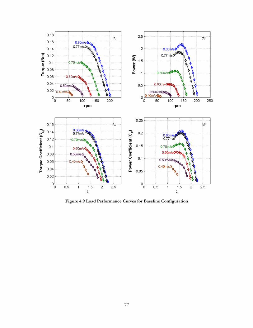
77
Figure 4.9 Load Performance Curves for Baseline Configuration
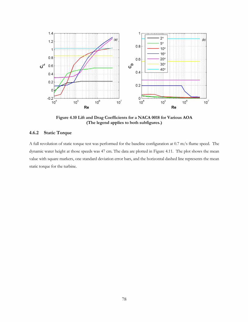
78
Figure 4.10 Lift and Drag Coefficients for a NACA 0018 for Various AOA (The legend applies to both subfigures.)
4.6.2 Static Torque
A full revolution of static torque test was performed for the baseline configuration at 0.7 m/s flume speed. The
dynamic water height at those speeds was 47 cm. The data are plotted in Figure 4.11. The plot shows the mean
value with square markers, one standard deviation error bars, and the horizontal dashed line represents the mean
static torque for the turbine.

79
Figure 4.11 Static Torque Curve for Baseline Configuration
Within the large standard deviation of this test data, there is a repeating pattern of torque as a function of
position, corresponding to the 90 degree sweep of the turbine blades. As the turbine azimuthal position
approaches 70° (and every 90° thereafter due to symmetry), the value for torque coefficient drops below 0.02.
The low torque position was observed for all four blades. Examining the stream-wise position view of the
turbine in Figure 4.12, it is not immediately obvious as to the reason for the loss of static torque.

80
Figure 4.12 Upstream View of Turbine with Respect to Static Torque
To investigate what may be causing the drop in torque at the 70° position, it is helpful to look at the static
torque coefficient for a single blade, with drawings of position added to help illustrate the results, as in Figure
4.13. As the figure shows, the static torque for a single blade is maximum as the blade is retreating toward the
downstream end of rotation and is located at the 100° position. The blade profile with respect to stream-wise
flow maximizes capability of drag force to produce positive torque in this location. Static torque turns negative
as the blade is advancing and reaches a minimum at 230° when the blade is fully extended to the full turbine
radius (providing maximum lever arm for the drag force). It is apparent from this examination that drag force
is dominant in starting the turbine from rest.

81
Figure 4.13 Single Blade Static Torque
If the performance of a single blade is replicated four times, with each curve offset successively by 90° from the
previous, the performance of a full turbine is simulated but without any wake effects from upstream blades
affecting downstream blades. The simulated, superpositioned turbine performance is compared to actual
turbine performance in Figure 4.14. As the figure shows, the general trend of static torque for the
superpositioned turbine follows the performance of the actual turbine, but there are positions of significant
deviation, both to the benefit and detriment of actual turbine static torque. The low static torque at the 70°
position is not predicted by the superpositioned turbine.

82
Figure 4.14 Comparison of Baseline Turbine Performance to Single Blade Superposition Square markers – average value for experimental data point.
Horizontal dashed line – mean for turbine.
The conclusion is that wake effects are responsible for the difference in performance. A re-examination of the
turbine position at 70° reveals the reason for lower static torque: the blade generating negative torque is
unobstructed and is near the location of maximum lever arm, and the blade generating positive torque is
partially obstructed by an upstream blade, leading to a turbulent wake and reduced velocity at the downstream
blade. It appears that the torque loss is inherent in the Four-Bladed Turbine design.
Figure 4.15 Wake Effects on Turbine Static Torque
One interesting observation resulting from the increased spread of torque readings is that the turbine, when not
fixed into position, can begin rotating even if the mean static torque for that position is lower than that required
to overcome starting torque, because instantaneous static torque may be above the starting torque threshold.
θ=0 θ=20 θ=40 θ=70
Static torque near maximum Static torque
drops
Unobstructed (-T) Blade
Partial Obstruction of (+T) Blade at Location of Best Drag

83
4.6.3 Tilted Turbine Test
Torque, power, torque coefficient, and power coefficient curves for the baseline configuration test are shown in
Figure 4.16.
Figure 4.16 Turbine Tilt Angle Performance for Baseline Configuration
The results show a consistent pattern: up through a tilt angle of 10°, there is a decreasing power coefficient with
increased angle of tilt. As Table 4.2 shows, there is a larger drop in performance from 5° to 10° than from 0° to
5°, suggesting that performance degradation as a function of tilt angle is superlinear.

84
Table 4.5 Baseline Configuration Tilt Angle Comparison
It is proposed that the performance degradation of the turbine is due both to effective loss of flow from the
angle that the stream-wise flow makes with the airfoil profile, as well as increased tip loss due to flow through
the strut ends.
4.6.4 Start-up and Shut-Down Test
A sample result of testing is shown in Figure 4.17 for the minimum loading case at 40° reference angle. Two
notable effects are the delay between the time of starting of the flume and the time that the turbine began to
rotate, and false start of the turbine at ~30 seconds corresponding to the turbine sticking at a low torque
position.
Strut Design
Tilt Angle
(degrees)
Actual CP
Loss
0 0.0%
2.5 -5.6%
5 -8.8%
10 -23.0%
Baseline
Configuration
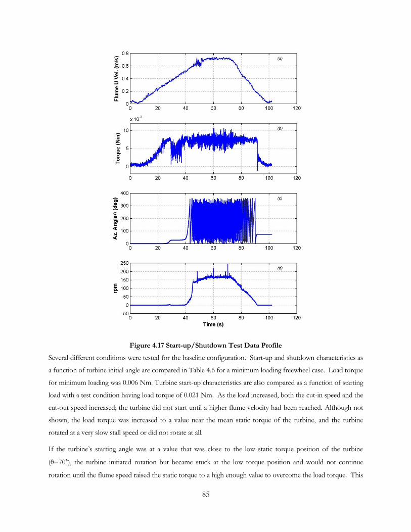
85
Figure 4.17 Start-up/Shutdown Test Data Profile
Several different conditions were tested for the baseline configuration. Start-up and shutdown characteristics as
a function of turbine initial angle are compared in Table 4.6 for a minimum loading freewheel case. Load torque
for minimum loading was 0.006 Nm. Turbine start-up characteristics are also compared as a function of starting
load with a test condition having load torque of 0.021 Nm. As the load increased, both the cut-in speed and the
cut-out speed increased; the turbine did not start until a higher flume velocity had been reached. Although not
shown, the load torque was increased to a value near the mean static torque of the turbine, and the turbine
rotated at a very slow stall speed or did not rotate at all.
If the turbine’s starting angle was at a value that was close to the low static torque position of the turbine
(θ=70°), the turbine initiated rotation but became stuck at the low torque position and would not continue
rotation until the flume speed raised the static torque to a high enough value to overcome the load torque. This

86
phenomenon was observed for starting angles of θ=30° up through θ=70°, an example of which is shown in the
data from Figure 4.17 that started at θ=40°. At other positions the turbine’s inertia was sufficient to carry it
through the low torque position and the turbine began to spin up at a lower cut-in speed, as was the case for the
θ=0°-30° and θ=80° cases. This is analogous to the performance of a straight-bladed Darrieus turbine in
operation. The difference in the cut-in speeds is readily noticed in the data from Table 4.6.
No significant differences are observable in cut-out speed for any initial starting positions, but cut-out speed did
increase for higher loading, as expected. Cut-out speed in general was lower than cut-in speed due to the
presence of induced velocity.
Table 4.6 Baseline Configuration Cut-In and Cut-Out Speeds
4.6.5 Turbine Wake
Wake velocities for each of the test conditions were non-dimensionalized by dividing the mean velocity by the
freestream velocity of the flume. For this test condition the freestream velocity was assumed to be u0=0.78
m/s, although not measured directly (only one ADV available for measurement), based on prior testing at the
same water height and pump frequency. The most similar test data taken was for the static case at the farthest
upstream point of the bow wake, which gives a mean velocity of 0.780 m/s. Therefore, the assumption of
u0=0.78 m/s is reasonable. Dividing through by u0, the non-dimensional velocities for all three cases are
compared directly in Figure 4.18.
When the turbine is operating, there is a small increase in velocity in the crosswise positive y-direction and the
spanwise positive Z-direction. The increase in crosswise velocity is likely due to crosswise momentum imparted
onto the flow by the turbine blade rotation direction. Also, immediately downstream of the turbine the wake
velocity in the stream-wise X-direction is near zero but increases to a fraction of the freestream velocity in the
far wake. The near wake deficit corresponds to the low-pressure recirculation region behind the turbine. Behind
the recirculation region the fluid gains momentum once again in the stream-wise direction, with a deficit due to
Starting Angle Load Torque (Nm) Cut-In Speed (m/s) Cut-Out Speed
0 0.006 0.47 0.21
10 0.006 0.47 0.21
20 0.006 0.47 0.21
30 0.006 0.58 0.22
40 0.006 0.60 0.20
50 0.006 0.57 0.19
60 0.006 0.60 0.23
70 0.006 0.55 0.18
80 0.006 0.47 0.23
0.53 0.21
0 0.021 0.71 0.38
Average cut-in/cut-out speed at 0.006
Nm load torque:

87
power extraction and turbulent mixing losses. Upstream of the turbine there is a decrease in velocity due to the
increased pressure from flow stagnation.
For the static case there is a smaller reduction in the stream-wise velocity downstream of the turbine. In fact, in
the near wake of the turbine there is an increase in flow velocity, due to flow acceleration around the turbine
blades.
For the static condition the turbine is producing less drag on the flow since it is not rotating; the only drag is the
profile drag on the blades. Less momentum is lost to turbulence, and consequently the recovered far wake
stream-wise velocity is higher than in operating conditions. The no-load condition, which includes losses from
not only frame drag and turbine profile drag but also increased losses from turbulent mixing, has a higher wake
velocity deficit than the static condition at all points. Finally, when power extraction is also included, the
maximum efficiency case causes the highest wake velocity deficit downstream of the turbine.

88
Figure 4.18 Non-Dimensionalized Wake Velocity
An experimental value for the wake velocity ratio is estimated for the wake data for the maximum efficiency
operating condtion by dividing the freestream velocity by the wake velocity of the farthest downstream
measurement point:
. (4.12)

89
4.7 Design Considerations
Several design parameters were tested to determine optimum configuration for generating torque and power.
These design parameters include the following:
Number of blades of the turbine, comparing the baseline configuration Four Bladed Turbine to the
Three-Bladed Turbine;
Strut design geometry, comparing a spoke arm design to a circular plate design;
Strut thickness, comparing two spoke arms of thickness 2.0 mm to 4.8 mm;
Shaft diameter, comparing turbine internal shaft diameters of 0, 6.4 mm, and 12.7 mm;
Turbine solidity, comparing a 15% solid turbine to a 30% solid turbine.
Load performance tests, static torque tests, and/or tilted turbine tests were performed to compare the design
configurations. The results are presented in each respective section.
4.7.1 Number of Blades and Helical Pitch
The turbines compared are the Three-Bladed Turbine and Four-Bladed Turbine, each, with a 6.4 mm central
shaft and spoke strut with width of 4.8 mm. The spoke edges were rounded to a radius roughly 1/2 the
thickness of the spoke. Photographs of the turbine configurations is shown in Figure 4.19. Each turbine has the
same solidity ratio (30%) and cross-sectional area (0.04 m2). The Three-Bladed Turbine has a 43.7° helical pitch
angle, while the Four-Bladed Turbine has 60.0° helical pitch angle.
(a) (b)
Figure 4.19 Turbine Design Comparison Configurations (a) Three-Bladed Turbine, (b) Four-Bladed Turbine
Figure 4.20 shows the load performance load performance curves of the two designs. The results indicate that
the Four-Bladed Turbine design outperforms the Three-Bladed Turbine design by a significant margin, although
their freewheel tip speed ratios are nearly the same.

90
Figure 4.20 Performance Comparison of Three- and Four-Bladed Turbines
As the two turbines have the same cross-sectional area, solidity, surface finish, and spoke thickness, the superior
torque and power for the Four-Blade Turbine may be due to the difference in helical pitch. Shiono et al. (2002)
determined from experiments that helical turbines with 40% solidity had performance increased as helical pitch
angle increased; the results from the present experiments agree with those results. Physically, the blade geometry
is more parallel to the incoming flow velocity for a turbine with lower helical pitch, which may be reducing lift
force generated at the blade and thus reducing performance. One would expect, then, that a blade with no
helical curve, i.e. as for a Darrieus turbine, would have superior power performance compared to a helical blade,
which is consistent with Shiono et. al. (2002) experimental results. In other words, the helical shape that
improves starting characteristics comes at a cost to peak efficiency.
The characteristics of operation in the flume for the Three-Bladed Turbine were noticeably different than that
of the Four-Bladed Turbine. As the Three-Bladed turbine was loaded to near stall velocity with higher flume
velocities (0.7-0.8 m/s), there was considerable instability of the test setup. Although the wake characteristics
were not measured for this turbine, it was observed that the turbine wake had a lower water column height and
seemingly slower wake speed. Vortex formation in the flume return duct intake was problematic, which in turn
caused pump output and thus flume inflow height and velocity to oscillate.
Additionally, the dynamics of turbine stall were different for the Three-Bladed Turbine. Rather than a quick
stall to zero angular velocity, the Three-Bladed turbine slowly decelerated and sometimes re-attained steady state
at a lower torque and rpm. The “partial stall” data points are not plotted, as they were somewhat unstable.
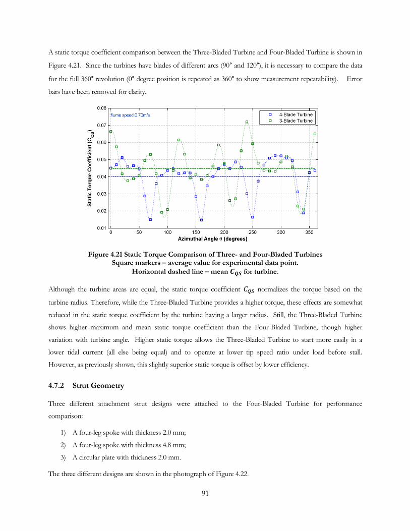
91
A static torque coefficient comparison between the Three-Bladed Turbine and Four-Bladed Turbine is shown in
Figure 4.21. Since the turbines have blades of different arcs (90° and 120°), it is necessary to compare the data
for the full 360° revolution (0° degree position is repeated as 360° to show measurement repeatability). Error
bars have been removed for clarity.
Figure 4.21 Static Torque Comparison of Three- and Four-Bladed Turbines Square markers – average value for experimental data point.
Horizontal dashed line – mean for turbine.
Although the turbine areas are equal, the static torque coefficient normalizes the torque based on the
turbine radius. Therefore, while the Three-Bladed Turbine provides a higher torque, these effects are somewhat
reduced in the static torque coefficient by the turbine having a larger radius. Still, the Three-Bladed Turbine
shows higher maximum and mean static torque coefficient than the Four-Bladed Turbine, though higher
variation with turbine angle. Higher static torque allows the Three-Bladed Turbine to start more easily in a
lower tidal current (all else being equal) and to operate at lower tip speed ratio under load before stall.
However, as previously shown, this slightly superior static torque is offset by lower efficiency.
4.7.2 Strut Geometry
Three different attachment strut designs were attached to the Four-Bladed Turbine for performance
comparison:
1) A four-leg spoke with thickness 2.0 mm;
2) A four-leg spoke with thickness 4.8 mm;
3) A circular plate with thickness 2.0 mm.
The three different designs are shown in the photograph of Figure 4.22.

92
(a) (b) (c)
Figure 4.22 Strut Design Comparison Configurations (a) 2.0 mm spoke (b) 4.8 mm spoke (c) Circular plate
Figure 4.23 shows a direct comparison of the performance of the 4-bladed turbine with the three different
designs.
Figure 4.23 Strut Design Performance Comparison
There was a noticeable difference in the performance of the turbine with the three different designs. The
circular plate design was the most efficient configuration, generating the highest torque and power coefficients.
This is likely due to two factors, described as follows.
The four-leg spokes each have faces that are moving in a direction that is perpendicular to the turbine
rotation of motion and that are adding profile drag resistance to the turbine, whereas the circular plate
contributes only skin friction drag to the resistance of motion. Although the circular plate has more

93
material and thus would have a higher skin friction drag as it revolves, the skin friction drag coefficient
is less than that of the profile drag coefficient. This is consistent with the experimental results of
Hoerner (1965).
A ducting effect of the circular plates improves the lift coefficient performance of the blade ends (Reid,
1925), whereas for the four-leg spoke designs, water is able to flow above or below the blade ends,
causing a blade tip effect loss that adversely affects the lift performance.
The thin four-leg spoke performed better than the thicker four-leg spoke, with power coefficients of 21% and
16%, respectively. The spoke arms for the two designs had the same width. Minimizing spoke thickness is
desirable because it results in lower profile drag; as the test results show, performance degradation can be
substantial.
4.7.3 Shaft Diameter
Shafts of three different diameters were compared to assess the effect of shaft profile drag and vortex shedding
on the performance of the turbine. The different shaft diameters were tested on the Four-Bladed Turbine with
2.0 mm four-leg spokes:
1) Turbine with no central shaft;
2) Turbine with 6.4 mm central shaft;
3) Turbine with 12.7 mm central shaft.
For each design the shafts are supported radially and spanwise at both ends by radial ball bearings and stationary
frame structure. The same bearing size and type are used for all three conditions. For the no-shaft design a
shaft stub of 6.4 mm diameter at each end of the turbine connects each spoke strut to the bearing, housing and
frame. To accommodate the 12.7 mm shaft, a transitional coupling is installed to transition from the 6.4 mm
shaft at the bearings to the 12.7 mm shaft going through the turbine. Additionally, to accommodate the larger
shaft, a separate hub connector with at 12.7 mm inner diameter bore is required. A set of photographs showing
the three turbines assembled with the different shaft diameters is shown in Figure 4.24.

94
(a) (b) (c)
Figure 4.24 Shaft Design Comparison Configurations (a) No central shaft (b) 6.4 mm shaft (c) 12.7 mm shaft
Figure 4.25 shows a direct comparison of the performance of the Four-Bladed Turbine with the three different
shaft diameters.
Figure 4.25 Shaft Design Performance Comparison
The data indicates that there is no significant difference in the performance of the turbine with the three
different shaft diameters. The performance curves are so similar that the differences are within the uncertainty
of the test measurements. Qualitatively, the no-shaft turbine was more unstable and experienced increased
deflection on it axis of rotation due to the fact that it had no central through-shaft to provide structural support.
The increased deflection did not result in significant performance impacts, however.

95
4.7.4 Tilt Angle
The Four-Bladed Turbine with circular plate was also compared to the baseline configuration (with 2.0 mm
four-leg strut) to compare the impact of strut/plate design on tilt angle performance. The torque and power
coefficient curves for both designs are shown in Figure 4.26. (The 4.8 mm strut performance was not compared
for this test, as it is assumed that its performance trend with respect to the baseline configuration is understood
from Load Performance Test results).
The results indicate that the circular plate strut design is clearly superior in reducing performance losses. For the
turbine with circular plates, there is a 9% efficiency loss for a 10° tilt; for the turbine with spokes, the efficiency
loss is 23%. The reduction in performance loss for the circular plate design may be due to a channeling of the
flow to be normal to the axis of rotation, whereas for the spoke design the flow continues on its stream-wise
path, impacting the blades at a yawed angle, with fluid passing through the gaps in the spokes.

96
Figure 4.26 Tilt Angle Performance Comparison
Some performance drop is expected simply due to the fact that the stream-wise velocity is incident on the
turbine blades at an angle that is not parallel to the blade profile plane. This effectively reduces the incoming
velocity according to Equation (4.1):
, (4.1)
where is the tilt angle and is the component of freestream velocity parallel to the turbine blade profile. A
plot of the trend in maximum power coefficient versus flume speed for a zero-degree tilt is shown in Figure

97
4.27. If the effective flume velocity is reduced per Equation (4.1), and the efficiency reduction is solely a
function of effective flume velocity, then the turbine performance reduction as a function of tilt angle should
follow the curves of Figure 4.27, and there should be a minor reduction in performance as shown in Table 4.7.
On the contrary, testing demonstrates that the turbine performance loss is much greater than that predicted
solely by the loss of velocity component in the blade direction. This suggests that the incidence angle may be
changing the effective blade profile significantly from a NACA 0018, and/or that tip loss may be significant.
Figure 4.27 Maximum Power Coefficient as a Function of Flume Velocity
Table 4.7 Power Coefficient Loss from Tilt Angle Prediction versus Actual
4.7.5 Solidity Comparison
To compare effects of solidity on performance, a Low Solidity Turbine was built to compare to the Three-
Bladed Turbine with solidity ratios of 15% and 30% respectively, each with three blades of the same profile. A
photograph of the Low Solidity Turbine is provided in Figure 4.28.
Strut Design
Tilt Angle
(degrees)
Tilt
Velocity
Predicted
CP Loss
from
cos(Tilt)
Actual CP
Loss
0 0.720 0.0% 0.0%
2.5 0.719 -0.2% -5.6%
5 0.717 -0.7% -8.8%
10 0.709 -2.8% -23.0%
0 0.720 0.0% 0.0%
2.5 0.719 -0.2% -4.5%
5 0.717 -0.8% -4.4%
10 0.709 -3.3% -8.9%
Baseline
Configuration
2 mm Circular
Plate
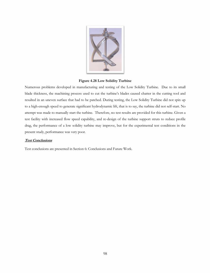
98
Figure 4.28 Low Solidity Turbine
Numerous problems developed in manufacturing and testing of the Low Solidity Turbine. Due to its small
blade thickness, the machining process used to cut the turbine’s blades caused chatter in the cutting tool and
resulted in an uneven surface that had to be patched. During testing, the Low Solidity Turbine did not spin up
to a high-enough speed to generate significant hydrodynamic lift, that is to say, the turbine did not self-start. No
attempt was made to manually start the turbine. Therefore, no test results are provided for this turbine. Given a
test facility with increased flow speed capability, and re-design of the turbine support struts to reduce profile
drag, the performance of a low solidity turbine may improve, but for the experimental test conditions in the
present study, performance was very poor.
Test Conclusions
Test conclusions are presented in Section 6: Conclusions and Future Work.
99
5 Vortex Model Results
A free-vortex model obtained from Sandia National Laboratories (SNL) is modified to simulate the helical
turbine performance. The SNL vortex model provides a unique opportunity to access a modified version of the
Strickland et al. (1981a) 3-D vortex model. Additionally, the model’s use of vortex theory to resolve velocities
induced on the turbine blades makes it unique among the traditional numerical models discussed in Section 3 in
being able to predict differences in performance between helical and straight-blade geometries. The SNL model
is named CACTUS (Code for Axial and Cross-flow Turbine Simulation) and is an adaptation of the Sandia
VDART3 code developed by Strickland et al. (1981a), currently written in FORTRAN F95 (M. Barone, Sandia
National Laboratories, personal communication, 8 July 2011). Strickland’s model was tested and verified against
experimental data for low solidity straight-bladed Darrieus turbines (Strickland et. al., 1981b) and incorporates
empirical treatments for pitching and dynamic stall.
A review of the literature suggests that this is the first implementation of a helical turbine in a vortex model.
Additionally, the micropower turbine has a higher chord-to-radius ratio than previous validation cases.
Strickland et al. (1981b) compared model results to experimental data for Darrieus turbines with chord-to-radius
ratios of 0.10 to 0.15. A comparison by Dai et al. (2011) for the performance of the vortex model for chord-to-
radius ratio of 0.36 found the vortex model to give unreasonably high performance predictions (up to 58%)
compared to actual performance (33%). The chord-to-radius ratio of the helical four-bladed turbine in the
present study is 0.47.
The goal of the modeling is to gain insight into the experimental results, predict performance of a full-scale
turbine for inflow velocities exceeding 0.8 m/s, and to assess the capability of the vortex model to provide
accurate predictions for a high chord-to-radius ratio turbine.
5.1 Model Parameters
The vortex model resolves the wake velocity and turbine force, torque, and power coefficients by solving the
system of equations described in Section 3.3. As described in the following sub-sections, several input
parameters to the model are required to specify the geometry, the operating configuration, and empirical
treatment of secondary effects (e.g., pitch rate). Many of the operational parameters were varied to evaluate
model sensitivity in comparison to experimental results.
Operational Parameters
Operational parameters are set to provide a balance between convergence capability and computational time to
achieve accurate results in approximately 20 minutes or less per data point (i.e., point on the -λ curve). This
enables substantially faster design iterations than a 3-D Navier-Stokes CFD simulation.

100
The model is set to solve for a cross-flow turbine (axial flow turbines being the other possible configuration).
The turbine was divided into 8 segments per blade and was run for 15 revolutions, at 18 time increments per
revolution.
The model generates vortices for each blade segment at each time increment. Initial revolutions run faster, but
do not provide an accurate measure of performance because turbine wake, consisting of the sum of shed and
trailing vortices, has not yet fully developed. An example of the model convergence for a well-converging test
point is shown in Figure 5.1.
Figure 5.1 Model Convergence for Successive Revolutions
Example shown is for the prototype turbine at u0=0.8 m/s with λ=1.6
To speed up computational time, the model allows for removal of the vortices from the calculation once they
are advected far enough downstream that their impact on turbine performance is minimal. The cutoff point was
set to 5 turbine radii downstream and this was found to not impact the model results in comparison to
calculating all shed vortices within 25 radii. The model also allows for a ground wall plane and shear layer and
calculating effects due to wall panel strength and vertical velocity variations – these options were not enabled in
order to model turbine performance in an unconfined, uniform flow. Although the experimental turbine was
installed in a walled flume with moderate blockage ratio, the model cannot represent sidewalls; this would be a
complex addition to the model that is beyond the scope of the present investigation, but is a possible line of
future work. Additionally, the model does not allow for inclusion of free surface effects. However, free surface
effects are only likely to be important at higher Froude numbers and blockage ratios than under the present
investigation. The model terminates when the difference between two successive revolutions’ average power
calculations ( ) meets the following criterion:
101
, (5.1)
where the subscript N denotes the revolution number. If, after 15 revolutions, the model does not meet the
criterion of Equation (5.1), the model terminates, and the average of the last 5 revolutions is used as the
revolution average (this commonly occurs at higher tip speed ratios).
Tip speed ratio and turbine rpm are input into the model and are varied for each model run to generate power
and torque curves for the turbine. The value for rpm is pre-calculated based on desired resource velocity
according to Equation (5.2).
(5.2)
Secondary Effects Parameters
The CACTUS model has two different dynamic stall models built in, only one of which can be selected for a
given model run: the Boeing-Vertol implementation, as outlined in Section 3.5.2, and the Leishman-Beddoes
implementation. After evaluating both implementations, the Boeing-Vertol model was chosen, as it caused less
variation per revolution. Pitch rate effects are implemented that capture changes in the location of effective
lift and drag on the hydrofoil due to pitching motion (Gormont, 1973). The smaller prototype-scale turbine
experiences high pitch rates due its high angular velocity (e.g., ~150 rpm); and enabling the correction for pitch
rate effects resulted in much closer agreement with experimental data for some configurations. Flow curvature
effects are implemented according to a modified version of the Mandal & Burton (1994) methodology as
outlined in Section 3.5.3 to better simulate the high chord-to-radius ratio of the turbine – when implemented
these were also found to improve model-experiment comparison for some conditions.
Geometric Parameters
Turbine geometric parameters that are input into the model include the turbine radius, blade profile, chord-to-
radius ratio, number of blades, blade height-to-radius ratio ( ), and blade mount point ratio. Table 5.1 gives
the values of geometric parameters input into the model for the prototype scale and full-scale turbines – the
only difference between the two being the turbine radius which, therefore, results in a lower rotational rate for
the same inflow condition and tip speed ratio for the larger turbine.
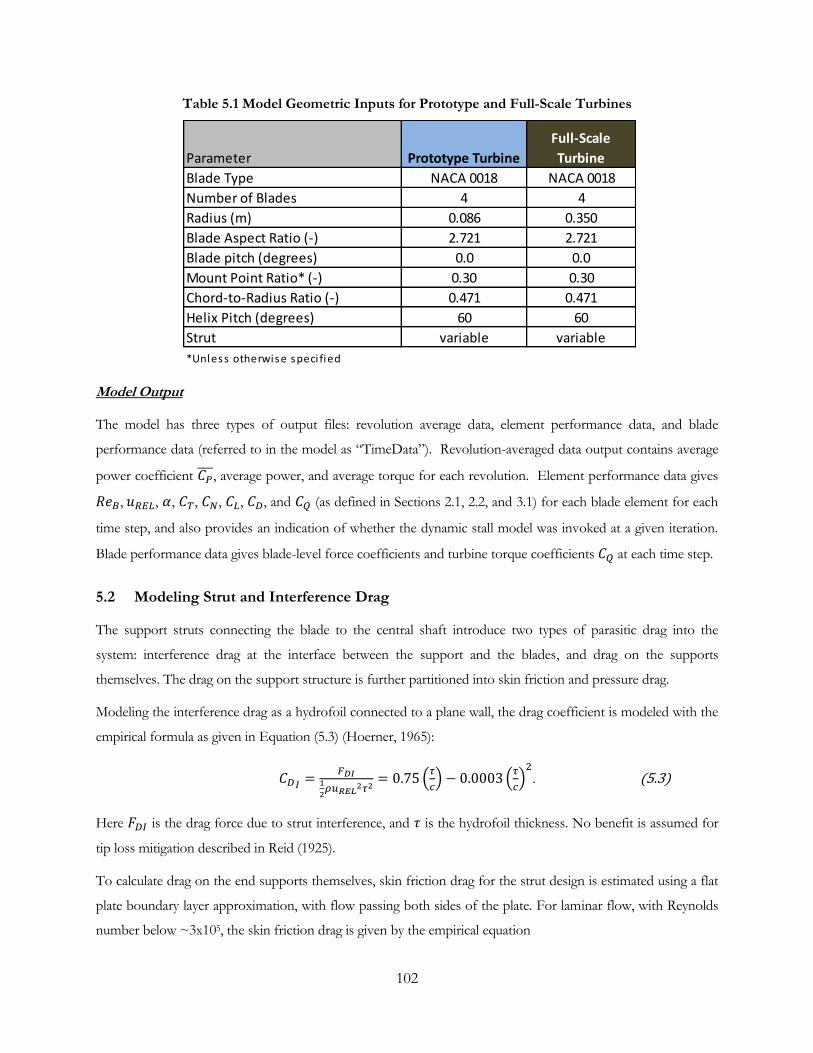
102
Table 5.1 Model Geometric Inputs for Prototype and Full-Scale Turbines
Model Output
The model has three types of output files: revolution average data, element performance data, and blade
performance data (referred to in the model as “TimeData”). Revolution-averaged data output contains average
power coefficient , average power, and average torque for each revolution. Element performance data gives
, , , , , , , and (as defined in Sections 2.1, 2.2, and 3.1) for each blade element for each
time step, and also provides an indication of whether the dynamic stall model was invoked at a given iteration.
Blade performance data gives blade-level force coefficients and turbine torque coefficients at each time step.
5.2 Modeling Strut and Interference Drag
The support struts connecting the blade to the central shaft introduce two types of parasitic drag into the
system: interference drag at the interface between the support and the blades, and drag on the supports
themselves. The drag on the support structure is further partitioned into skin friction and pressure drag.
Modeling the interference drag as a hydrofoil connected to a plane wall, the drag coefficient is modeled with the
empirical formula as given in Equation (5.3) (Hoerner, 1965):
. (5.3)
Here is the drag force due to strut interference, and is the hydrofoil thickness. No benefit is assumed for
tip loss mitigation described in Reid (1925).
To calculate drag on the end supports themselves, skin friction drag for the strut design is estimated using a flat
plate boundary layer approximation, with flow passing both sides of the plate. For laminar flow, with Reynolds
number below ~3x10⁵, the skin friction drag is given by the empirical equation
Parameter Prototype Turbine
Full-Scale
Turbine
Blade Type NACA 0018 NACA 0018
Number of Blades 4 4
Radius (m) 0.086 0.350
Blade Aspect Ratio (-) 2.721 2.721
Blade pitch (degrees) 0.0 0.0
Mount Point Ratio* (-) 0.30 0.30
Chord-to-Radius Ratio (-) 0.471 0.471
Helix Pitch (degrees) 60 60
Strut variable variable
*Unless otherwise speci fied

103
(laminar), (5.4)
where is the laminar strut drag coefficient and ReC is the strut chord Reynolds number (Fox & McDonald,
1998), calculated as
. (5.5)
The variable is the strut chord length. For turbulent flow, the drag coefficient becomes
(turbulent). (5.6)
The turbulent drag coefficient values are valid for Reynolds numbers below 109 (Fox & McDonald, 1998).
Pressure drag for the strut designs is approximated as a two-dimensional elliptical object. Hoerner (1965)
described an empirical equation for the strut drag for laminar flow in terms of the skin friction coefficient as
(laminar), (5.7)
where is the strut thickness. The corresponding turbulent pressure drag is given by
(turbulent). (5.8)
5.3 Adaptations for a Helical Turbine
Revisions to CACTUS are made to accommodate the turbine’s helical geometry. As opposed to a straight-
bladed Darrieus turbine, for which each blade segment only varies with vertical (spanwise) position, the helical
turbine design in the present study has segments whose ends and center vary in all three dimensions from blade
element to blade element. This requires a change to the model operation to accommodate the yawed blade.
Figure 5.2 shows the model segments both a helical and straight blade and illustrates the three-dimensional
variation of the helical blade endpoints.

104
Figure 5.2 Model Blade Segmentation and Endpoint Variation
For the helical blade, the blade element cut is in the horizontal plane as shown in Figure 5.2. This is done to
keep all of the blade elements identical and because the NACA 0018 blade lies in the horizontal plane. To allow
the use of the NACA 0018 lift and drag tables, the incoming velocity vectors and blade profile are also resolved
with respect to the horizontal plane.
The complexity of the helical turbine with respect to a vortex model analysis becomes apparent, however, when
analyzing the vorticity vectors generated for each blade segment. For a straight vertical blade, the vortex
filament as shown in Figure 3.4, which is aligned with the blade element geometry in the vertical direction, is
also normal to the incoming velocity direction; therefore no correction is required to the value of circulation per
the Kutta-Joukowski theorem (see Section 3.2, Equation (3.17)). However, for the helical blade, the blade
element is not vertical but rather slanted to the complementary angle to the helical pitch angle (i.e. (90°- )).
Therefore it is not normal to incident velocity on the NACA 0018 blade element profile. In this case, a
correction to the Kutta-Joukowski theorem is made to correct for the yaw. Applying the Independence
Principle (Bull & Dekkers, 1989) to the blade element results in the conclusion that the vortex that is shed from
the blade element will be in the direction of the element filament and will have strength that is proportional to
the component of the velocity that is normal to the filament. The component of velocity normal to the filament
is found by taking the sine of the helical pitch angle and results in the correction as seen in Equation (3.18).
5.4 Prototype Turbine Modeling
The geometric parameters of the prototype turbine model, as shown in Table 5.1, are input into the model to
provide comparison to the experimental data of the Four-Bladed Turbine.
The importance of secondary effects in the modeling is evident by examination of the model prediction curves
of Figure 5.3. As the figure shows, with dynamic stall, pitch rate, and flow curvature effects disabled, the model

105
predicts a negative power coefficient for the configuration that produced =+24% in experimental data.
As each secondary effect is added successively, the model output improves until it becomes quite similar to the
test data with all secondary effects enabled (except for the stall region at low tip speed ratio).
Figure 5.3 Model Output Demonstrating Impact of Secondary Effects Test Data is for prototype Four-Bladed Turbine with circular plate
ends at =0.8 m/s.
One discrepancy between the model and the prototype scale experimental turbine is that the model input for
blade mount point ratio is 0.3, but the design of the experimental prototype turbine has mount point of 0.5
(tangent to rotation at ½- chord). As shown in Figure 5.4, preliminary model runs indicated that the model had
high variability for MP>0.30. The dashed lines in this figure and subsequent plots represent areas where
the model had high variability or otherwise suspect results and are shown only to illustrate the model output.
Dashed line regions should not be considered valid data.

106
Figure 5.4 Prototype Turbine Model Results for Different Mount Point Ratio With all secondary effects included; (a) Power coefficient (b)
Variation in power coefficient. Dashed lines represent regions of poor model output.
The power coefficient is shown in Figure 5.4(a) for several mount point ratios, and Figure 5.4(b) shows the
variation of the over the last 5 revolutions of each model run, according to Equation (5.9):
. (5.9)
The high variability is viewed as an issue with the model physical simulation, since the results most likely do
not reflect actual turbine operation. The poor prediction arises due to the corrections made by secondary effects
(flow curvature, dynamic stall, and pitch rate effects), which are shown to be driving the physics of the model
prediction. This is discussed in detail in Section 5.5.
5.4.1 Model Prediction of Strut Drag Effects
The vortex model results were compared to the prototype Four-Bladed Turbine performance at 0.8 m/s for
three different strut designs: 2.0 mm circular plate, 2.0 mm four-leg strut and 4.8 mm four-leg strut. The
secondary effects and mount point ratio are implemented as follows:
Boeing Vertol dynamic stall – activated;
Pitch rate effects – activated;
Flow curvature – activated;

107
Mount point ratio – 0.30.
The results are shown in Figure 5.5. In the figure, solid lines represent model predictions, overlain on the
experimental results, show with diamond markers. The model accurately predicts the change in turbine
performance, but does not predict the shift in the tip speed ratio at which occurs. The model
implements strut drag by subtracting it from the tangential force after the model has already converged; therefore
strut drag cannot alter the operating speed of the device. Also, shed vortex strength is determined based solely
on the lift coefficient; therefore, the struts also do not contribute to the wake evolution. The effect of strut drag
in the model is to reduce for any operating speed. This differs from the actual performance as seen in the
experimental results, where additional strut drag not only decreases performance, but also shifts to a
lower tip speed ratio.
Figure 5.5 Vortex Model Prediction of Strut Drag Effects Diamonds represent experimental data, with a spline fit represented
by dashed lines. Solid lines are vortex model prediction. Green is turbine with 2.0 mm circular plates, blue is with 2.0 mm spokes,
black is with 4.8 mm spokes.
5.4.2 Model Prediction with Varying Inflow Velocity
Model predictions for the four-bladed turbine with 2.0 mm circular plates were compared to experimental
results for three inflow velocities: 0.6 m/s, 0.69 m/s, and 0.8 m/s, as shown in Figure 5.6. The secondary
effects and mount point ratio are implemented as follows:
Boeing Vertol dynamic stall – activated;
Pitch rate effects – activated;
Flow curvature – activated;

108
Mount point ratio – 0.30.
At inflow velocity of 0.8 m/s, the model accurately predicts the magnitude of and the corresponding tip
speed ratio . However, as the inflow velocity is reduced, the model fails to correctly predict the loss in
power and predicts a much higher performance than the experiments. The model also does not predict the shift
in toward lower . This is may be due to the increased relative influence of strut and bearing friction
drag at lower velocities for the experimental results.
Figure 5.6 Vortex Model Prediction for Varying Inflow Velocity Diamonds represent experimental data, with a spline fit represented by dashed lines. Solid lines are vortex model prediction. Blue is data
at 0.8 m/s, black is 0.69 m/s, green is 0.60 m/s.
The model predicts stall much closer to than the experimental results show. One explanation for this
phenomenon may be due to turbulence. As shown in experimental results by Bachant (2011), introducing
turbulence into the flow field of a cross-flow turbine resulted in a shift in the stall point to a lower tip speed
ratio, while the value of was unaffected. The turbine blades are creating a turbulent wake, and the
interaction of the following blades with this turbulent wake may be delaying stall to a lower tip speed ratio. The
vortex model predictions do not capture this effect.
5.4.3 Prediction of Prototype Turbine Performance at Higher Flow Speeds
The inflow velocity was extrapolated to determine if the model predicts a performance increase corresponding
to operating at higher inflow velocity. In the transitional Reynolds number regime corresponding to inflow
velocities of 0.6-0.8 m/s, i.e., Re=5x10⁴ to 1x10⁵, the change in lift coefficient per change in Reynolds number

109
for a NACA 0018 blade profile is large and positive (as shown Figure 4.10); therefore as
velocity is increased, one would expect the overall performance to increase due to improved lift. This trend is
observed in the steadily increasing observed as inflow velocity is increased in the experimental results
(see Figure 4.9, for example).
The vortex model also predicts an increase in as shown in Figure 5.7 for 1.5 m/s flow as compared to
the lower 0.8 m/s flow rate. For this simulation, the secondary effects and mount point ratio are implemented
as follows:
Boeing Vertol dynamic stall – activated;
Pitch rate effects – activated;
Flow curvature – activated;
Mount point ratio – 0.30.
The model does predict that turbine performance will continue to increase as flume velocity is increased. The
performance predicted by the model at the higher velocity is reasonably close to Gorlov’s (1998) previous claims
of efficiency for a helical turbine around 35%. However, based on the disagreement between experimental and
numerical results for different inflow velocities in Figure 5.6, the magnitude of the predicted performance
increase should be viewed with caution.

110
Figure 5.7 Prototype Turbine Model Extrapolation to Inflow Velocity of 1.5 m/s MP=0.30. Blue line represents model prediction at 0.8 m/s, black is
at 1.5 m/s. Dashed lines represent regions of poor model output.
At 1.5 m/s inflow, for extrapolated predictions at , the model reverses the trend in , with mean
beginning to increase; also, the error increases significantly. To determine the reason for the deviation from
expected results requires an examination of the secondary effects of flow curvature, pitch rate, and dynamic stall,
as is described in Section 5.5.
5.5 Impact of Secondary Effects on Model Performance
As was demonstrated in Figure 5.3, implementation of secondary effects is crucial to providing a model
prediction that matches experimental data. However, it was also shown in Section 5.4.3 that at times the model
prediction with secondary effects implemented results in a prediction with high variability in the revolution-
averaged power coefficient (i.e., demonstrates a lack of convergence). This section further inspects the impact
of secondary effects.
A plot of the torque coefficient and half-chord angle of attack for a few revolutions of the model with turbine
operating at is shown in Figure 5.8. A tip speed ratio of 2.6 represents a condition where the model is
deviating from expected results and is providing a higher than expected, with a high error (i.e., high
variability from revolution to revolution). In Figure 5.8(a), the model is shown with all secondary effects,
including flow curvature, activated. In Figure 5.8(b), the results are shown for the same condition with flow
curvature disabled, but with dynamic stall and pitch rate effects active.

111
Figure 5.8 Effect of Flow Curvature at High Tip Speed Ratio
For prototype turbine operating at =2.6 and =1.5 m/s (a) with flow curvature active (b) with flow curvature disabled
Comparing the two figures, it is evident that the flow curvature implementation is causing significant variability
in the turbine torque prediction, which is leading to variability in the predicted output. This effect is caused
by the flow curvature correction. For positive angle of attack, the flow curvature correction adds to the turbine
performance when the lift coefficient slope is positive and decreases turbine performance when the lift
coefficient slope is negative (i.e., at initial stall). For negative angle of attack, the effect is opposite, with turbine
performance increased in the area of initial stall and decreased otherwise. As seen in Figure 5.8(a), flow
curvature greatly decreases performance when the blade element angle of attack has exceeded the stall angle on
the upstream pass (i.e., α>~12°), and increases performance when the stall is exceeded on the downstream pass

112
(i.e., α<~(-12°)). When the performance is enhanced, strong vortices are shed off of the turbine blade elements,
resulting in increased instability in the results as the vortex is shed and advected downstream.
The flow curvature correction implemented by Mandal & Burton was based on the pre-stall thin airfoil theory
lift slope, where the correction to lift coefficient is given by
. (5.10)
In the present model the implementation is modified to make use of lift and drag lookup tables for a
NACA0018 blade such that lift and drag coefficient correction is found by
, (5.11)
where the lift and drag coefficients are found using static lookup tables implemented at the ¼-chord.
The Mandal & Burton (1994) flow curvature implementation provides no specific direction for how to
implement flow curvature effects in the stall region. Further research is needed to determine the effects of flow
curvature in the stall region to determine if a correction to the Mandal & Burton methodology is required.
Although the implementation of flow curvature has been shown to cause the variability in predicted ,
disabling flow curvature does not result in a better prediction of the magnitude of . With flow curvature
effects enabled, at =2.6, the predicted is 0.46, but with flow curvature effects disabled, the predicted value
is reduced only to 0.43, which is still unrealistically high for this turbine geometry. The erroneously high
magnitude arises because of the calculations made for dynamic stall and pitch rate effects. In the model, pitch
rate effects are estimated by reassigning the location of angle of attack calculation for lift and drag from the ¼-
chord position to the following positions:
Lift coefficient is calculated from α at the ¾-chord position;
Lift coefficient is assigned to the ½-chord position;
Drag coefficient is calculated from α at the ½-chord position and assigned to the ½-chord position.
These approximations were used by Strickland in the vortex model (Strickland et al., 1981(b))) and are valid for
turbines with small chord-to-radius ratios. However, for large chord-to-radius ratios, the ¼-chord, ½-chord,
and ¾-chord positions have larger differences in their respective angles of attack because of the greater
difference in their relative velocity vectors. The result is a lag between when the blade enters lift stall versus drag
stall. This is shown for the prototype turbine extrapolated velocity condition with =2.6 in Figure 5.9, which
zooms in on a single revolution of the turbine, with flow curvature effects disabled. The figure highlights the
part of the revolution that experiences high torque coefficient , which is responsible for the high power
coefficient prediction. In the highlighted region, at maximum performance, is ~10°, while is ~6°; the
difference between the two is due to high chord-to-radius ratio.
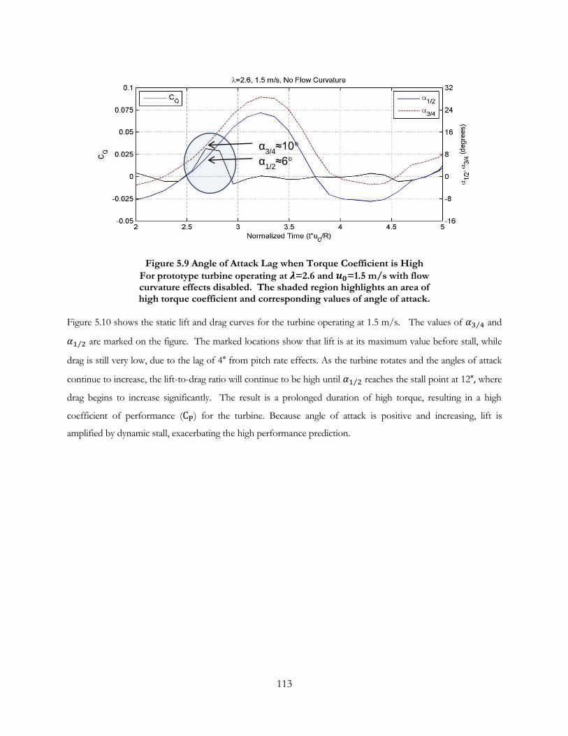
113
Figure 5.9 Angle of Attack Lag when Torque Coefficient is High
For prototype turbine operating at =2.6 and =1.5 m/s with flow curvature effects disabled. The shaded region highlights an area of high torque coefficient and corresponding values of angle of attack.
Figure 5.10 shows the static lift and drag curves for the turbine operating at 1.5 m/s. The values of and
are marked on the figure. The marked locations show that lift is at its maximum value before stall, while
drag is still very low, due to the lag of 4° from pitch rate effects. As the turbine rotates and the angles of attack
continue to increase, the lift-to-drag ratio will continue to be high until reaches the stall point at 12°, where
drag begins to increase significantly. The result is a prolonged duration of high torque, resulting in a high
coefficient of performance ( ) for the turbine. Because angle of attack is positive and increasing, lift is
amplified by dynamic stall, exacerbating the high performance prediction.
α3/4≈10°
α1/2≈6°

114
Figure 5.10 Angle of Attack Lag Shown on Static Lift and Drag Coefficient Curves
For prototype turbine operating at =2.6 and =1.5 m/s with flow curvature effects disabled. The makers show the operating point for
the position of interest.
The high prediction of torque due to pitch rate effects and dynamic stall has been noted in previous research.
Mandal & Burton (1994) noted that the dynamic stall model predictions differed highly from experimental data
under some conditions. For a similarly-sized Darrieus turbine (0.45 m) and similar inflow velocity (1.45 m/s),
Dai et al. (2011) observed that the vortex model predicted nearly double the power coefficient compared to
experimental results. Some effort has been made to correct the model with a dynamic stall dampening
methodology (Cardona, 1984), but this empirical correction has not been implemented in the present study.
It is seen that the secondary effects of dynamic stall, pitch rate, and flow curvature, while small in magnitude for
small chord-to-radius ratio turbines, are greatly enhanced for high chord-to-radius ratio turbines, to the point
where they are driving the physics of the model solution.
5.6 Prediction of Performance of the Full-Scale Turbine
The model was also used to predict performance of the full-scale four-bladed turbine; the turbine has radius of
0.7 m but otherwise the same non-dimensional geometric parameters as the prototype. The secondary effects
are implemented as follows:
Boeing Vertol dynamic stall – activated;
Pitch rate effects – activated;
Flow curvature – activated.
As Figure 5.11 indicates, the model predicts an unreasonably high performance as compared to that which is
generally observed for cross-flow turbines, curves that do not represent the traditional curve shape, and a

115
value that at some speeds approaches or exceeds the Betz limit of . The only change to geometry
from the prototype turbine is the size of the turbine, which affects blade Reynolds number and rotational rate.
As Reynolds number is dependent on chord length, the full-scale turbine with longer chord will experience a
higher ReB than the prototype turbine, scaled by a factor of approximately 4.1, the ratio of their chord lengths.
To maintain the tip speed ratio of the prototype turbine, the rotation rate must also decrease inversely with the
turbine radius.
Figure 5.11 Full-Scale Turbine Model Predictions with All Secondary Effects Active u0=1.5 m/s. Dashed lines represent regions of poor model output.
Operating at the higher Reynolds number results in a higher for the full-scale turbine; is further amplified
by dynamic stall, biasing due to flow curvature and the pitch lag between and from pitch rate effects.
Pitch rate effects are dependent to 1st order on the rotation rate of the turbine; therefore, one would expect
pitch rate effects for the full-scale turbine to be decreased in magnitude compared to the prototype turbine. It is
not possible to conclude without further examination, however, whether pitch rate effects can be neglected
altogether for the lower rotational speed.
Model predictions with pitch rate and flow curvature effects disabled are shown in Figure 5.12. The secondary
effects are implemented as follows:
Boeing Vertol dynamic stall – activated;
Pitch rate effects – disabled;
Flow curvature – disabled.

116
With pitch rate effects disabled, is calculated at the ¼ chord for both lift and drag, eliminating the pitch lag
between the two. With the pitch rate and flow curvature effects disabled, the model curve resembles that of a
typical hydrokinetic turbine curve. However, there is still considerable variability, which is caused by
strong vortices shed from the blades whose strength is amplified by dynamic stall. Due to the high
variability, the model results cannot be relied upon as accurate prediction, particularly since some secondary
effects have been disabled, but are shown to demonstrate the influence of secondary effects and the need for
their further refinement.
Figure 5.12 Full-Scale Model Predictions with Pitch Rate and Flow Curvature Disabled u0=1.5 m/s. Dashed lines represent regions of poor model output.
5.7 Summary
As discussed in Chapter 3, vortex models, such as CACTUS, offer a potentially attractive compromise between
blade element momentum (BEM) and CFD models. Vortex models can capture more of the hydrodynamics
than momentum models, but at a fraction of the computational expense of CFD models. However, for novel
turbine designs, empirical correction factors (i.e., secondary effects) in common use may not be suitable. For the
high-solidity turbine simulated here, flow curvature, pitch rate, and dynamic stall lead to unrealistic turbine
performance for some conditions. Further, the results indicate that basic work is needed to understand the limits
of these correction factors and develop suitable modifications for higher solidity turbines.
117
6 Conclusions and Future Work
This section presents the major conclusions of this thesis with regard to micropower system analysis, turbine
and parameter selection, experimental testing, and turbine modeling. Opportunities for future work are also
identified.
6.1 Accomplishments and Conclusions
Micropower System Analysis
This thesis has outlined the components required for a tidal micropower system generating power on the order
of 20 Watts. The system is intended for use in small-scale submerged applications where the tidal resource has
peak currents of 1.5 m/s or greater, although installations in lower tidal currents are possible if less power is
required. System power requirements will depend on loads, which for the present study have been approximated
as a set of oceanographic instruments and embedded computing devices. Required system components include
turbine, generator, gearbox, controller, power converter and battery bank, some of which may be integrated into
a single unit (e.g., controller and power converter for MPPT). Prior to development of a full system, complete
characterization of the components is required to understand how they will integrate to obtain required power
output. Turbine generator torque and rpm matching has been highlighted as an aspect of the analysis critical to
the success of the system. The low rotational rates of a hydrokinetic turbine with low inflow velocity make it
difficult to drive a generator without the use of a gearbox to step up the rpm, but a direct drive system may be
desirable to increase overall system reliability. A permanent magnet axial flux generator has been suggested as a
possible component that may facilitate a direct drive system.
To determine approximate system capability for a given tidal current, a steady state system model was created
that determines battery charge and system power output over a long-term deployment. System component
models use either commercially available data for a specific component or an estimated performance curve as a
placeholder if a specific component has not been identified. The model results show that a system
incorporating a helical turbine with area of ~0.7m2 could provide approximately 15 W continuous power for
instrumentation. This value is likely to change, and system model fidelity will be improved, as specific
component models are incorporated.
Turbine Selection and Parameter Optimization
The component of focus in the present study is the hydrokinetic turbine. Several common turbine designs have
been examined, including drag devices (e.g., Savonius rotor), lift devices (e.g., Darrieus, helical, and axial flow
turbines), and hybrid devices that include both lift and drag features. The chosen design is the helical cross-flow
turbine, which offers the advantages of self-start and smooth torque output, while still maintaining a reasonably
high level of efficiency. The important parameters in design of a helical turbine include blade profile and pitch,
118
helical pitch angle, aspect ratio, number of blades, blade wrap, and strut design. Prior experimental testing or
computational analysis is used to determine the best design configuration where possible, taking into account
manufacturability and size constraints.
Experimental Testing
Prior research has not addressed best practices of some design choices, and in such cases, experimental
prototypes were developed to test turbine performance. Testing of the turbine prototypes is performed in a
water flume with maximum inflow velocity of 0.8 m/s. Three prototype turbines were tested, including three-
bladed turbines with helical pitch angle of 43.7° and solidities of 30% and 15%, respectively, and a four-bladed
turbine with helical pitch angle of 60° and 30% solidity. A performance test of each turbine determined power
coefficient ( ) and torque coefficient ( ) as a function of tip speed ratio (λ) for several inflow velocities, and a
static torque test measured torque for a stationary turbine as a function of azimuthal angle. Turbine attachment
options tested include two different end-strut designs of varying thickness and a circular endplate. Central
shafts of varying thickness were also tested, including a case with no central shaft. A tilted turbine test
measured performance degradation when the turbine was installed with its rotating axis tilted toward the
freestream direction by a small angle to simulate a deployment on a cobble or angled slope. Some turbine wake
velocity measurements were also made along the turbine centerline in the stream-wise direction, upstream and
downstream of the turbine. The following bullets provide a summary of the conclusions from experimental
turbine testing:
Helical Pitch/Number of Blades
For the flume speeds tested, the Four-Bladed Turbine with a 60° helical pitch angle is more efficient than
the Three-Bladed Turbine with 43.7° helical pitch angle, despite the two turbines having the same blade
profile, solidity ratio, and cross-sectional area. The additional blade allows for a higher pitch angle with
smaller increase in aspect ratio. Average static torque coefficient for the Three-Bladed Turbine is
moderately higher than that of the Four-Bladed Turbine; the Three-Bladed Turbine also has a higher
variation of static torque coefficient. Neither turbine had difficulty with self-start; therefore, the trade-off
between starting torque and performance clearly favors the Four-Bladed Turbine.
Strut Design
Strut design is critical to maximizing turbine performance. A thicker strut design results in lower power
performance due to increased pressure drag; thus, strut width should be minimized. A circular plate
provides the most efficient blade attachment, most likely due to elimination of pressure drag. The circular
plate design also reduces performance losses during a tilted deployment of up to 10 degrees.
119
Shaft Diameter
Shaft diameter thickness has a negligible effect on turbine performance for shaft diameters up to 7% of the
turbine diameter (which is the ratio for the 12.7 mm shaft on the 172 mm diameter turbine). A turbine with
no central shaft provides similar performance to a turbine with a central shaft, but is more prone to
deflection and wobbling during rotation. Therefore, a central shaft is best for increasing strength and
stability.
Solidity Ratio
Solidity ratio comparison at low flume speeds favors a turbine with higher solidity. The low solidity turbine
(15% solidity versus 30% for other variants) could not self-start in flow speeds up to 0.8 m/s, whereas the
higher solidity turbines had no difficulty with self-starting in flow speeds of 0.5 m/s. Performance of the
low solidity turbine would be expected to improve with the more efficient strut design or at higher flume
speeds.
General Performance Observations
Maximum power performance of the turbines from experimental testing was 24.0% for the Four-
Bladed Turbine (R=0.086 m, AR=1.36, , NACA 0018 blades, , ) with circular
plate struts.
Maximum power coefficient was observed to increase as flume speed increased due to operation in the
transitional Reynolds number regime. It is hypothesized that this increase should level off as inflow
speed is increased further.
To increase self-start capability, turbines should be allowed to start up freely with minimal loading.
Loading should be applied when the turbine has reached freewheel rotation rate.
Despite a blade wrap ratio of 100%, static torque varies significantly with azimuthal angle, but remains
positive at all azimuthal positions. The static torque for a turbine cannot be estimated solely from the
superposition of torque from a single blade mirrored about the central axis of rotation. In addition to
azimuthal positioning, upstream blade wake effects and blade “ducting” acceleration effects likely are
the cause for the difference between the analysis of single blade superposition and actual static turbine
performance.
Turbine cut-in speed depends on the angle at which the turbine rests prior to starting – the closer the
static turbine angle is to a low torque position, the more likely the cut-in speed will increase. Cut-out
speed is less than cut-in speed because the turbine’s induced velocity and inertia allows it to delay stall.

120
Turbine Modeling Conclusions
A vortex model was used to model the turbine performance and to gain insight into experimental results. Vortex
model theory posits that blade segments can be represented as vortex generators, and that bound, shed and
trailing vortices influence the local blade velocities and thus overall turbine performance. The model captures
the geometry of the helical turbine and incorporates secondary effects of dynamic stall, pitch rate, and flow
curvature. The model, CACTUS, was provided by Sandia National Laboratories and is an updated version of
the original Sandia VDART3 model. The vortex model is unique among the cross-flow turbine numerical
models in that it can resolve the differences between a helical turbine and a similar straight-bladed Darrieus
turbine and can more accurately describe the turbine wake to predict performance. The vortex model was used
to derive simulated performance curves for the prototype turbine operating at several velocities and with each of
the three attachment methods. Test runs predicting prototype performance at 1.5 m/s, and simulation of the
full-scale turbine at 1.5 m/s inflow velocity were also performed.
The following are the conclusions made with respect to the vortex model predictions.
Model Reliability
The vortex model has provided predictions that are reasonably close to experimental results for some
cases. However, it is evident for some conditions that the model provides unreasonably high
predictions with high variability in the revolution-averaged power coefficient, particularly at high tip
speed ratio and high mount point ratio. This is due to the implementation of secondary effects into the
model, which, for high chord-to-radius ratio turbines, are driving the physics of the solution. Prior
research and the present study, however, indicate that the secondary effects are crucial to accurately
predicting the performance of a turbine with a large chord-to-radius ratio.
The high prediction is due to the empirical correction factors and the calculation of , , and at
(different) discrete positions that are used to model the secondary effects of dynamic stall and pitch
rate. The Boeing Vertol dynamic stall model may also be over-predicting lift, which further exacerbates
inaccuracies in the pitch rate and flow curvature corrections for high solidity turbines.
The high variability in the model prediction is attributed to flow curvature effects in the initial blade
stall region of a revolution and also to amplification of performance by the dynamic stall model. For a
turbine with small chord-to-radius ratio, chord length is insignificant compared to the arc of rotation
traced by the blade, and the difficulties encountered here would be lessened. The over-amplification of
lift, particularly at high tip speed ratio produces strong shed vortices due to the Kutta-Joukowski
implementation, which contributes to high variability.

121
Model comparison to experimental results
The model provides reasonable comparison of the prototype turbine performance in terms of peak tip
speed ratio and the general performance curve at flume speed of 0.8 m/s.
The model accurately represents the magnitude of loss of turbine performance due to strut drag, but is
incapable of predicting the shift in tip speed ratio for maximum that results from increasing strut
drag in experiments.
The model predicts a decrease in turbine performance coefficient at slower inflow velocity, but under-
predicts the magnitude of decrease and does not predict an observed shift in the tip speed ratio for
maximum performance. It is hypothesized that strut and bearing friction drag are more influential at
the lower tip speed ratio, an effect which is not accurately represented by the model.
Actual stall occurs at a lower tip speed ratio than predicted by the model; it is hypothesized based on
prior research results (Bachant, 2011) that this may be due to turbulence effects that are not captured by
the model.
All simulations are performed at a lower mount point ratio (MP=0.30) than is actually implemented in
the prototype design (MP=0.50), due to model instability for mount point ratios greater than 0.35.
Secondary effects are responsible for the unrealistic efficiency predictions and lack of convergence from
revolution to revolution.
Performance Extrapolation
The model predicts an increase in turbine performance for the prototype turbine operating at 1.5 m/s
compared to 0.8 m/s. This is consistent with the expectation that higher inflow velocity and higher
blade Reynolds number will increase turbine lift coefficient and improve efficiency. The model
convergence does degrade for , however, due to the influence of secondary effects.
Experimental testing or alternative numerical model prediction of the full-scale performance testing is
necessary to evaluate the accuracy of these results.
The model does not provide stable results for the full-scale turbine due to secondary effects. De-
activating the pitch rate effects and flow curvature for the full-scale turbine provided a more reasonable
curve but did not improve the variability in revolution averaged power coefficient. Dynamic stall
appears to be driving the simulation variability.
6.2 Future Work
This thesis has worked to design and characterize a helical cross-flow tidal turbine, which is part of a tidal
micropower system. Future work should continue the process of system component selection, design, and
refinement. There are many challenges ahead. Designer selection of a high-efficiency generator that operates at
122
low rpm and low starting torque, with corollary analysis to determine the optimum gear ratio, is a challenge that
must be overcome to ensure success of the overall system design. Increasing the system predicted power output
to match the desired 20 W continuous at 1.5 m/s peak current will also provide some challenging work. An
efficient and compatible battery set, power converter, and control scheme are also needed. Custom design of a
device to provide optimized control (e.g., MPPT tracking) could be considered. Updates to the existing steady
state system performance model will naturally follow from component selection and characterization.
Development and testing of a full-scale prototype turbine is required to determine any performance changes
resulting from scaling the turbine. As the Stevenson-Eroglu flume size and speed limitations preclude testing of
the full-scale turbine, an alternate test location and method will be required. This will determine the suitability of
using prototype testing as a predictor of full-scale turbine performance.
An improved method is needed for determining any blockage effects resulting from testing the turbine in the
narrow flume. A robust analysis should provide a method for accurately predicting any performance
improvement based on knowing turbine solidity, tip speed ratio, blockage ratio, Froude number and Reynolds
number. To validate the methodology, the prototype turbine should be tested in an open channel setup to
compare to experimental results obtained in the flume testing.
Future work could also concentrate on providing the next iteration of turbine design to improve performance
beyond what was obtained in the present study. Blade pitch angle and blade profile changes offer some
interesting possibilities for performance enhancement, with previous studies indicating that a toe-out angle or
cambered-out blade may provide superior results. Decreasing blade wrap coverage to increase pitch angle of the
blades could be investigated, although caution must to taken to avoid introducing self-start and oscillation issues
into the design (beyond those inherent to blade-to-blade interaction in cross-flow turbines). Determining the
optimum number of blades for peak power performance could be investigated by modeling or experiment.
Redesign and testing of a low-solidity turbine at higher flume velocity could provide insight into whether low
solidity turbines, which have lower torque coefficient but operate at higher peak tip speed ratios, may be
preferable for turbine-generator integration.
Further investigation into alternate turbine designs is recommended to determine if another design can offer
similar levels of power, torque, and self-start performance with increased ease of manufacture. A hybrid
Savonius-Darrieus turbine offers promising performance characteristics if designed properly. Novel designs,
such as a multi-stage Darrieus, or pseudo-helical turbine with straight, angled blades (rather than helical blades)
could also be considered.
Finally, further investigation into model predictions is necessary to provide an accurate turbine performance
predictor. CFD methods may provide the most accurate prediction but come at the expense of very large
computational times. Vortex, double-multiple streamtube, or cascade models will provide a fast, reliable

123
alternative if corrections to flow curvature, dynamic stall and pitch rate effects can be made to work interactively
and accommodate a high chord-to-radius ratio turbine. Further work is warranted to improve the secondary
effect models for high chord-to-radius turbines, which can be accomplished by combining theory, results from
CFD simulations, and experimental testing.

124
GLOSSARY OF SYMBOLS
Channel upstream area in streamtube Channel upstream area outside
streamtube Turbine cross-sectional area (= ) Wake cross-sectional area Channel area outside wake Channel far-wake area Turbine cross-sectional area Flume cross-sectional area Tidal constituent amplitude Blade planform area Turbine aspect ratio Blade aspect ratio Axial induction factor Wake velocity ratio Turbine blade quantity Drag coefficient Blade-strut interference drag coefficient
Laminar pressure drag coefficient (strut)
Turbulent pressure drag coefficient (strut)
Reference drag coefficient (dyn. stall)
Laminar skin friction drag coefficient
(strut) Turbulent skin friction drag coefficient
(strut) Lift coefficient Reference lift coefficient (dyn. stall)
Normal force coefficient Power coefficient
Revolution average power coefficient
Power coefficient of unblocked conditions
Variability in model revolution average
power coeffcientPower coefficient Maximum power coefficient
Unblocked maximum power coefficient
Torque coefficient
Static torque coefficient
Tangential force coefficient Blade chord length Turbine Diameter Savonius bucket Diameter Turbine axial force Turbine average axial force
Individual streamtube axial force
Drag force
Individual downstream streamtube axial force
Average upstream streamtube axial force Interference drag force Lift force Normal force Tangential force
Individual upstream streamtube axial force
Average upstream streamtube axial force Froude number Tidal constituent frequency Gear ratio gravitational constant Blade element spanwise height or vortex
filament height Upstream channel height Wake channel height Far wake remixed channel height Flume static water height Turbine height
Blade heave
Blade heave rate Current K Kinetic power density Dynamic stall constant Empirical coefficient (cascade model) Blade spanwise length Blade mount point ratio Model revolution number Number of blades (Cascade model) Mass flow rate Pressure drop across turbine Pressure difference across cascade P Power Average Power p+ Turbine upstream pressure p- Turbine downstream pressure Pressure drop across turbine Pressure drop across turbine Dynamic pressure Turbine radius Reynolds number Blade Reynolds number Strut chord Reynolds number

125
Machine Reynolds number Revolutions per minute Distance from point to vortex filament Strut chord length Torque Average torque Average downstream disc torque
Average upstream disc torque Static torque Generator torque Turbine torque (= ) Time Distance between blades (cascade model) Mean stream-wise velocity Stream-wise velocity Unit step function Freestream velocity (= ) Freestream velocity Component of freestream velocity normal
to tilted turbine Stream-wise velocity at turbine
(streamtube) Stream-wise velocity at downstream
turbine disc (streamtube) Stream-wise velocity at upstream turbine
disc (streamtube) Wake velocity Channel freestream velocity outside wake Channel far-wake re-mixed velocity Induced velocity from bound vortex Equilibrium velocity between streamtube
discs Vortex induced velocity on a point Relative velocity on a blade Rel. velocity of blade 2 (cascade model)
Rel. velocity of blade 3 (cascade model)
Stream-wise velocity at turbine Induced velocity from shed vortex Induced blade tip velocity Induced velocity from trailing vortex Circulation velocity correction (cascade
model) Mean crosswise velocity Crosswise velocity Mean spanwise velocity Spanwise velocity Stream-wise position Mount point distance from leading edge
Vortex circulation Bound vortex circulation Shed vortex circulation Trailing vortex circulation Angle of attack Rate of change of angle of attack Quarter chord angle of attack
Half chord angle of attack
Three-quarter chord angle of attack
Blade 2 angle of attack (cascade model) Blade 2 angle of attack (cascade model) Flow curvature angle of attack correction Leading edge angle of attack Reference angle of attack (dyn. stall) Trailing edge angle of attack Zero-lift angle of attack Azimuthal blade pitch (half chord) Quarter chord azimuthal blade pitch
Flow curvature angle of attack variation Dynamic stall constant Helical blade pitch Blockage ratio Gearbox efficiency Converter efficiency Per-stage gear efficiency Blade (element) azimuthal position Tidal constituent phase Blockage correction factor Tip speed ratio Tip speed ratio at maximum power
coefficient Blade wrap ratio Density Solidity ratio Chord-to-radius ratio Blade thickness Strut thickness Kinematic viscosity Turbine tilt angle Turbine angular velocity Turbine angular acceleration Generator angular velocity Turbine angular velocity (= )

126
REFERENCES
Alam, M. J. (2009). A low cut-in speed marine current turbine (Master’s Thesis). Memorial University of Newfoundland. Retrieved from www.engr.mun.ca/~tariq
Alam, M. J., & Iqbal, M. T. (2009). Design and development of hybrid vertical axis turbine. 2009 Canadian Conference on Electrical and Computer Engineering, CCECE ’09 (pp. 1178-1183).
Ampair Energy Ltd. (2010). UNDERWATER 100TM (UW 100TM) Operation Installation & Maintenance Manual
Manufactured by Ampair® (Issue 1.2). Ampair. Retrieved from www.ampair.com
Anderson, J. D. (2001). Fundamentals of Aerodynamics (3rd ed.). Boston: McGraw-Hill.
Bachant, P. (2011). Experimental investigation of helical cross-flow axis hydrokinetic turbines, including effects of waves and turbulence. (Master’s thesis). University of New Hampshire.
Buchmann, I. (2010a). Is lithium-ion the ideal battery? Retrieved February 8, 2012, from
www.batteryuniversity.com
Buchmann, I. (2010b). Lithium-based batteries. Retrieved February 8, 2012, from www.batteryuniversity.com
Buchmann, I. (2010c). Charging lithium-ion. Retrieved February 8, 2012, from
www.batteryuniversity.com
Buchmann, I. (2010d). Comparison Table of Secondary batteries. Retrieved February 15, 2012, from
www.batteryuniversity.com
Buchmann, I. (2010e). What’s the best battery? Retrieved February 15, 2012, from
www.batteryuniversity.com
Buchmann, I. (2011a). Charging lead acid. Retrieved February 8, 2012, from www.batteryuniversity.com
Buchmann, I. (2011b). Cost of power. Retrieved February 15, 2012, from www.batteryuniversity.com
Bull, M. K., & Dekkers, W. A. (1989). Vortex Shedding From Cylinders in Near Axial Flow. Tenth Australian Fluid Mechanics Confererence - University of Melbourne - 11-15 December 1989 (pp. 6.41-6.44). Melbourne, Australia.
Burton, T., Sharpe, D., Jenkins, N., & Bossayani, E. (2001). Wind Energy Handbook. Chichester: John Wiley & Sons.
Cardona, J. L. (1984). Flow curvature and dynamic stall simulated with an aerodynamic free-vortex model for VAWT. Wind Engineering, 8(3), 135-143.
Castelli, M. R., & Benini, E. (2011). Effect of blade inclination angle on a Darrieus wind turbine. Journal of Turbomachinery, 134(3).

127
Cetacean Research Technologies. (2011). Hydrophone Specifications (August 2011). Retrieved February 18, 2012, from www.cetaceanresearch.com
Chu, F.-Q., Chen, P., Shen, X.-X., & Yan, X.-H. (1985). Parameter selection of straight bladed vertical axis wind turbine. Alternative Energy Sources VI Volume 3 Wind/Ocean/Nuclear/Hydrogen: Proceedings of the Sixth Miami International Conference on Alternative Energy Sources, December 12-14, 1983, Miami Beach, Florida, USA (pp. 77-85). Washington, D.C.: Hemisphere Publishing Corporation.
Coy, J. J., Townsend, D. P., & Zaretsky, E. V. (1985). Gearing. NASA RP-1152; AVSCOM TR 84-C-15.
Dai, Y. M., Gardiner, N., Sutton, R., & Dyson, P. K. (2011). Hydrodynamic analysis models for the design of Darrieus-type vertical-axis marine current turbines. Proceedings of the Institution of Mechanical Engineers, Part M: Journal of Engineering for the Maritime Environment, 225(3), 295-307. doi:10.1177/1475090211400684
Dai, Y. M., & Lam, W. (2009). Numerical study of straight-bladed Darrieus-type tidal turbine. Proceedings of the Institution of Civil Engineers: Energy, 162(2), 67-76. doi:10.1680/ener.2009.162.2.67
Drela, M. (n.d.). XFOIL subsonic airfoil development system. Retrieved February 21, 2012, from web.mit.edu/drela/Public/web/xfoil/
Duquette, M. M., Swanson, J., & Visser, K. D. (2003). Solidity and blade number effects on a fixed pitch, 50W horizontal axis wind turbine. Wind Engineering, 27(3), 299-316.
Encoder Products Company. (2011). Model 15T thru-bore, Model 15H hollow bore. Retrieved February 12, 2012, from www.encoder.com
Epler, J. (2010). Tidal resource characterization from acoustic Doppler current profilers. (Master’s thesis). University of Washington.
Ferreira, C. J. S., Bijl, H., Bussel, G., & Kuik, G. (2007). Simulating dynamic stall in a 2D VAWT: Modeling strategy, verification and validation with particle image velocimetry data. Journal of Physics: Conference Series, 75. doi:0.1088/1742-6596/75/1/012023
Fiedler, A., & Tullis, S. (2009). Blade offset and pitch effects on a high solidity vertical axis wind turbine. Wind Engineering, 33(3), 237-246.
Fitzgerald, A. E., Kingsley, C., & Umans, S. D. (2003). Electric machinery. Boston, Mass: McCraw-Hill.
Fox, R. W., & McDonald, A. T. (1998). Introduction to Fluid Mechanics. New York: J. Wiley.
Futek. (n.d.). Futek Model TFF425 Flange to Flange Reaction Torque Sensor w/ Thru Hole, Drawing #
Fl1137-B. Retrieved February 12, 2012, from www.futek.com
Garrett, C., & Cummins, P. (2007). The efficiency of a turbine in a tidal channel. Journal of Fluid Mechanics, 588, 243-251.
Gieras, J. F., Wang, R.-J., & Kamper, M. J. (2004). Axial flux permanent magnet brushless machines. Dordrecht: Kluwer.

128
Gorlov, A. (1995). Unidirectional helical reaction turbine. U.S. Patent No 5,451,137. U.S. Patent and Trademark Office.
Gorlov, A. (1998). Development of the helical reaction hydraulic turbine: final technical report (DE-FGO1-96EE 15669). DOE/EE/15669-TI.
Gormont, R. E. (1973). A mathematical model of unsteady aerodynamics and radial flow for application to helicopter rotors. Fort Eustis, Virginia: Eustis Directorate, U.S. Army Air Mobility Research and Development Laboratory.
Hagerman, G., & Polagye, B. (2006). Methodology for Estimating Tidal Current Energy Resources and Power Production by Tidal In-Stream Energy Conversion (TISEC) Devices, Report# EPRI – TP – 001 NA Rev 3.
Hall, T. (2012). Numerical simulation of a cross flow marine hydrokinetic turbine. (Unpublished master’s thesis). University of Washington.
Hirsch, H., & Mandal, A. C. (1984). Flow curvature effect on vertical axis Darrieus wind turbine having high chord-radius ratio. Proceedings of the First European Wind Energy Conference (pp. 405-410). Hamburg.
Hirsch, H., & Mandal, A. C. (1987). A cascade theory for the aerodynamic performance of Darrieus wind turbines. Wind Engineering, 11(3), 1164-1175.
Hoerner, S. F. (1965). Fluid-dynamic drag: Practical information on aerodynamic drag and hydrodynamic resistance. Brick Town, N.J.: Self-published.
Islam, M., King, D., & Fartaj, A. (2007). Desirable airfoil features for smaller-capacity straight-bladed VAWT. Wind Engineering, 31(3), 165-196.
Islam, M., King, D., & Fartaj, A. (2008). Aerodynamic models for Darrieus-type straight-bladed vertical axis wind turbines. Renewable and Sustainable Energy Reviews, 12(4), 1087-1109.
Khan, M. J., Iqbal, M. T., & Quaicoe, J. E. (2010). Dynamics of a vertical axis hydrokinetic energy conversion system with a rectifier coupled multi-pole permanent magnet generator. Renewable Power Generation, IET, 4(2), 116-127. doi:10.1049/iet-rpg.2008.0123
Khan, M. N. I. (2008). A Micro Seafloor Marine Current Energy Conversion System. (Master’s thesis). Memorial University of Newfoundland. Retrieved from www.engr.mun.ca/~tariq.
Kirke, B. K. (1998). Evaluation of self-starting vertical axis wind turbines for stand-alone applications. (PhD Thesis). Griffith University, Australia.
Klimas, P., & Worstell, M. (1981). Effects of blade present pitch/offset on curved-blade Darrieus vertical axis wind turbine performance (SAND-81-1762). Albuquerque, NM: Sandia National Laboratories.
Kundu, P. K., Cohen, I. M., Ayyaswami, P. S., & Hu, H. H. (2008). Fluid Mechanics (4th ed.). Boston: Academic Press.
Leishman, J. G., & Beddoes, T. S. (1989). A semi-empirical model for dynamic stall. Jounal of the Americal Helicopter Society, 34(3), 3-17.

129
Mandal, A. C., & Burton, J. D. (1994). The effects of dynamic stall and flow curvature on the dynamics of Darrieus turbines applying the cascade model. Wind Engineering, 18(6), 267-282.
Menet, J.-L. (2004). Increase in the Savonius rotors efficiency via a parametric investigation. 2004 European Wind Energy Conference and Exhibition. London.
Migliore, P. G., Wolfe, W. P., & Fanucci, J. B. (1980). Flow curvature effects on Darrieus turbine blade aerodynamics. Journal of Energy, 4(2), 49-55.
Morshed, K. N. (2010). Experimental and numerical investigations on aerodynamic characteristics of Savonius wind turbine with various overlap ratios. (Master’s thesis). Georgia Southern University.
Moury, S. (2009). Design of low speed axial flux permanent magnet generators for marine current application. (Master’s thesis). Memorial University of Newfoundland. Retrieved from www.engr.mun.ca/~tariq.
National Aeronautics and Space Administration (NASA). (2009). UH-60 airloads program tutorial. Retrieved February 24, 2010, from halfdome.arc.nasa.gov
New Energy Corporation Inc. (n.d.). Encurrent hydro turbines 5 and 10 kW specifications. Retrieved February 8, 2012, from www.newenergycorp.ca
Nortek AS. (2010). Vector 3D Acoustic Velocimeter TS-050-en-06.2010. Retrieved February 12, 2012, from www.nortekusa.com
Orme, J. A. C., Masters, I., & Griffiths, R. T. (2001). Investigation of the effect of biofouling on the efficiency of marine current turbines. Proceedings of MAREC 2001 (pp. 91-99).
Owen, A., & Bryden, I. G. (2007). Energy extraction implications of structurally significant velocity variation in tidal currents. OCEANS 2007 - Europe (1-4244-0635-8, 978-1-4244-0635-7) (pp. 1-5).
Paraschivoiu, I. (1988). Double multiple streamtube model for Darrieus wind turbines. Journal of Propulsion and Power, 4(4), 370-377.
Pendergast, D. R., DeMauro, E. P., Fletcher, M., Stimson, E., & Mollendorf, J. C. (2011). A rechargeable lithium-ion battery module for underwater use. Journal of Power Sources, 196(2), 793-800.
Polagye, B. (2009). Hydrodynamic effects of kinetic power extraction by in-stream tidal turbines. (Doctoral dissertation). University of Washington.
Polagye, B., & Thomson, J. Tidal energy resource characterization: methodology and field study in Admiralty Inlet, Puget Sound, US. Submitted to the Proceedings of the Institution of Mechanical Engineers, Part A: J. Energy and Power.
Polagye, B., Van Cleve, B., Copping, A., & Keith, K. (Eds.). (2011). Environmental effects of tidal energy development. Proceedings of a Scientific Workshop. March 22-25, 2010. Silver Spring, Md: U.S. Dept. Commerce. NOAA tech. memo. NMFS-F/SPO-116.
RD Instruments. (2001). WorkHorse Monitor ADCP User’s Guide P/N 957-6165-00 (January 2001). Retrieved February 18, 2012, from www.comm-tec.com

130
Reddy, T. B., & Linden, D. (Eds.). (2011). Linden’s Handbook of Batteries (4th ed.). New York City: McGraw-Hill.
Reid, E. G. (1925). The Effects of Shielding the Tips of Airfoils. (NACA Report No. 201) (pp. 345-353). Washington, D.C.: U.S. Government Printing Office.
Reuter, R. C., & Worstell, M. (1978). Torque Ripple in a Vertical Axis Wind Turbine (SAND78-0577). Albuquerque, NM: Sandia National Laboratories.
RTD Embedded Technologies Inc. (2011). CMX32M cpuModules User’s Manual BDM-610000075 Revision
B. Retrieved February 17, 2012, from www.rtd.com
RTD Embedded Technologies Inc. (2010). SATA34106 SATA Drive Carrier User’s Manual BDM-610020085 Revision A. Retrieved February 17, 2012, from www.rtd.com
SES Flexcharge USA. (2002). MANUAL MODEL: NC25A-12(24, 36, 48) Ultra High Efficiency 25 Ampere
Alternative Energy Battery Charge Controller. Revision 2, Version 1. Retrieved from www.flexcharge.com
Sheldahl, R. E., & Feltz, L. V. (1980). Aerodynamic performance of a 5-metre-diameter Darrieus turbine with extruded aluminum NACA 0015 blades (SAND80-0179). Albuquerque, NM: Sandia National Laboratories.
Shiono, M., Suzuki, K., & Kiho, S. (2002). Output characteristics of Darrieus water turbine with helical blades for tidal current generations. Proceedings of The Twelfth (2002) International Offshore and Polar Engineering Conference (pp. 859-864). Kitakyushu, Japan.
Strickland, J. H. (1975). The Darrieus turbine: A performance prediction model using multiple streamtubes (SAND75-0431). Albuquerque, NM: Sandia National Laboratories.
Strickland, J. H., Webster, B. T., & Nguyen, T. (1979). A vortex model of the Darrieus turbine: an analytical and experimental study. Journal of Fluids Engineering, 101(4), 500-505.
Strickland, J. H., Smith, T., & Sun, K. (1981a). A user’s manual for the vertical axis wind turbine code VDART3 (SAND 81-7020). Albuquerque, NM: Sandia National Laboratories.
Strickland, J. H., Smith, T., & Sun, K. (1981b). A vortex model of the Darrieus turbine: an analytical and experimental study (SAND 81-7017). Albuquerque, NM: Sandia National Laboratories.
Templin, R. J. (1974). Aerodynamic performance theory for the NRC vertical-axis wind turbine (NAE Report LTR-LA-160).
Tregenza, N., & Chelonia Ltd. (2011). CPOD.exe: a guide for users (8 Oct 2011). Retrieved February 18, 2012, from www.chelonia.co.uk
Twidell, J., & Weir, A. D. (2006). Renewable Energy Resources (2nd ed.). London: Taylor & Francis.
Ushiyama, I., & Nagai, H. (1988). Optimum Design Configurations and Performance of Savonius Rotors. Wind Engineering, 12(1), 59-75.

131
Wakui, T., Tanzawa, Y., Hashizume, T., & Nagao, T. (1995). Hybrid Configuration of Darrieus and Savonius Rotors for Stand-Alone Wind Turbine-Generator Systems. Electrical Engineering in Japan, 150(4).
The World Factbook 2009. (2009). Washington, D.C.: Central Intelligence Agency.
Verdant Power, & GCK Technologies. (2005). Amesbury tidal energy project (ATEP) Integration of the Gorlov helical turbine into an optimized hardware/software system platform (April 30, 2005).
Worstell, M. (1978). Aerodynamic performance of the 17 meter diameter Darrieus wind turbine (SAND78-1737). Albuquerque, NM: Sandia National Laboratories.
Yuen, K., Thomas, K., Grabbe, M., Deglaire, P., Bouquerel, M., Österberg, D., & Leijon, M. (2009). Matching a permanent magnet synchronous generator to a fixed pitch vertical axis turbine for marine current energy conversion. IEEE Journal of Oceanic Engineering, 34(1), 24-31. doi:10.1109/JOE.2008.2010658

132
Appendix A: Prototype Turbine Manufacturing Details
The scale-model turbine blades were designed in Solidworks by creating a two dimensional curve from an
imported text file of two-dimensional (X,Y) data points of a NACA 0018 hydrofoil section. The data points
were scaled to the desired size of the turbine blades, then swept along a helix angle with desired height and pitch
angle. The Solidworks file was converted into G-code and a machining sequence was defined to produce a
blade from a solid rectangular block of aluminum.
A CNC 3-axis mill cut the rectangular block into blade shape. This required rotating the feedstock 180 degrees
on its lengthwise axis after completing one side of the blade to cut the other side. The blades were cut to an
accuracy of +/-0.13 mm. The blade ends were left attached to an extended portion of the original block to
complete the machining. The blade ends were cut to a rough angle using an angled miter saw, then
buffed/ground to the desired angle and length with higher precision. A female jig was used to hold the blade
for measuring blade length on a mill with digital readout to 0.0127 mm precision. Ensuring the blade end was
flush with the jig face ensured proper inclination angle of the blade.
The blades were attached to end plates or spoke arms using one or two counter-sunk screws. An optimal
combination of alignment and ease of assembly was accomplished by attaching one blade end with two screws
positioned along the blade chord line for alignment, and one screw on the other blade end to minimize chances
of misalignment of the other end. Attachment points on the blade end were precisely aligned using a temporary
alignment tab that was designed into the turbine spoke, as shown in Figure A.1. The alignment tab attached the
spoke assembly to the female jig. With the blade in the jig and the spoke alignment tab attached, the blade end
was centered and drilled. To ensure a smooth, consistent surface finish with low roughness, the cut blades were
sandblasted, primed and painted with 2-3 coats of gloss automotive paint. This also protected the blades from
corrosion during testing.
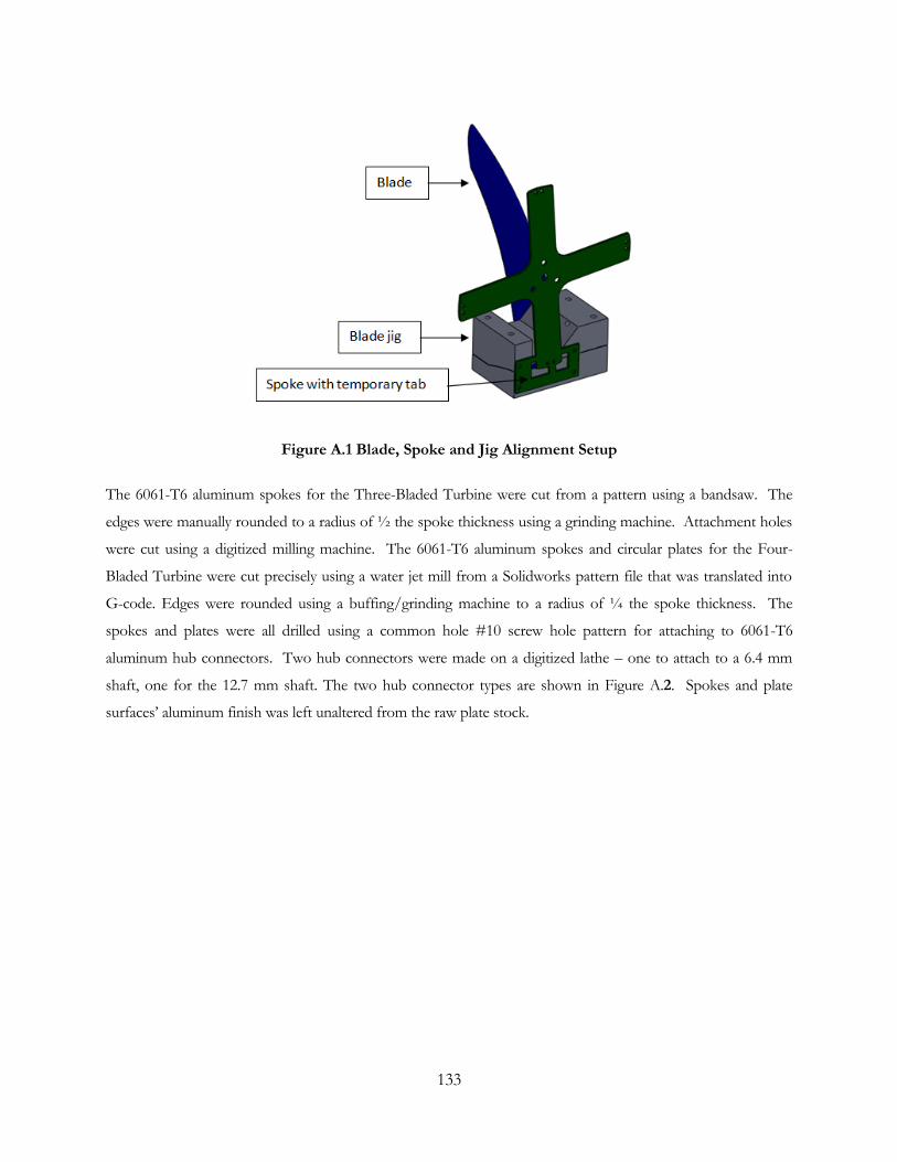
133
Figure A.1 Blade, Spoke and Jig Alignment Setup
The 6061-T6 aluminum spokes for the Three-Bladed Turbine were cut from a pattern using a bandsaw. The
edges were manually rounded to a radius of ½ the spoke thickness using a grinding machine. Attachment holes
were cut using a digitized milling machine. The 6061-T6 aluminum spokes and circular plates for the Four-
Bladed Turbine were cut precisely using a water jet mill from a Solidworks pattern file that was translated into
G-code. Edges were rounded using a buffing/grinding machine to a radius of ¼ the spoke thickness. The
spokes and plates were all drilled using a common hole #10 screw hole pattern for attaching to 6061-T6
aluminum hub connectors. Two hub connectors were made on a digitized lathe – one to attach to a 6.4 mm
shaft, one for the 12.7 mm shaft. The two hub connector types are shown in Figure A.2. Spokes and plate
surfaces’ aluminum finish was left unaltered from the raw plate stock.

134
Figure A.2 Hub Connectors and Shaft
The stainless steel or aluminum central shafts were cut to lengths for integration into the test setup. A rigid
aluminum coupling joined the turbine module shaft and the instrumentation module shaft. A lower flanged
stainless steel bearing was press fit onto the turbine shaft module. This allowed for easy installation and removal
of the turbine module from the test setup by simply loosening the rigid coupling and pulling the lower bearing
from the housing.
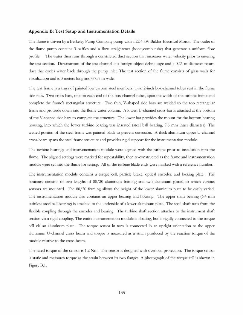
135
Appendix B: Test Setup and Instrumentation Details
The flume is driven by a Berkeley Pump Company pump with a 22.4 kW Baldor Electrical Motor. The outlet of
the flume pump contains 3 baffles and a flow straightener (honeycomb tube) that generate a uniform flow
profile. The water then runs through a constricted duct section that increases water velocity prior to entering
the test section. Downstream of the test channel is a foreign object debris cage and a 0.25 m diameter return
duct that cycles water back through the pump inlet. The test section of the flume consists of glass walls for
visualization and is 3 meters long and 0.757 m wide.
The test frame is a truss of painted low carbon steel members. Two 2-inch box-channel tubes rest in the flume
side rails. Two cross-bars, one on each end of the box-channel tubes, span the width of the turbine frame and
complete the frame’s rectangular structure. Two thin, V-shaped side bars are welded to the top rectangular
frame and protrude down into the flume water column. A lower, U-channel cross-bar is attached at the bottom
of the V-shaped side bars to complete the structure. The lower bar provides the mount for the bottom bearing
housing, into which the lower turbine bearing was inserted (steel ball bearing, 7.6 mm inner diameter). The
wetted portion of the steel frame was painted black to prevent corrosion. A thick aluminum upper U-channel
cross-beam spans the steel frame structure and provides rigid support for the instrumentation module.
The turbine bearings and instrumentation module were aligned with the turbine prior to installation into the
flume. The aligned settings were marked for repeatability, then re-constructed as the frame and instrumentation
module were set into the flume for testing. All of the turbine blade ends were marked with a reference number.
The instrumentation module contains a torque cell, particle brake, optical encoder, and locking plate. The
structure consists of two lengths of 80/20 aluminum framing and two aluminum plates, to which various
sensors are mounted. The 80/20 framing allows the height of the lower aluminum plate to be easily varied.
The instrumentation module also contains an upper bearing and housing. The upper shaft bearing (6.4 mm
stainless steel ball bearing) is attached to the underside of a lower aluminum plate. The steel shaft runs from the
flexible coupling through the encoder and bearing. The turbine shaft section attaches to the instrument shaft
section via a rigid coupling. The entire instrumentation module is floating, but is rigidly connected to the torque
cell via an aluminum plate. The torque sensor in turn is connected in an upright orientation to the upper
aluminum U-channel cross beam and torque is measured as a strain produced by the reaction torque of the
module relative to the cross-beam.
The rated torque of the sensor is 1.2 Nm. The sensor is designed with overload protection. The torque sensor
is static and measures torque as the strain between its two flanges. A photograph of the torque cell is shown in
Figure B.1.
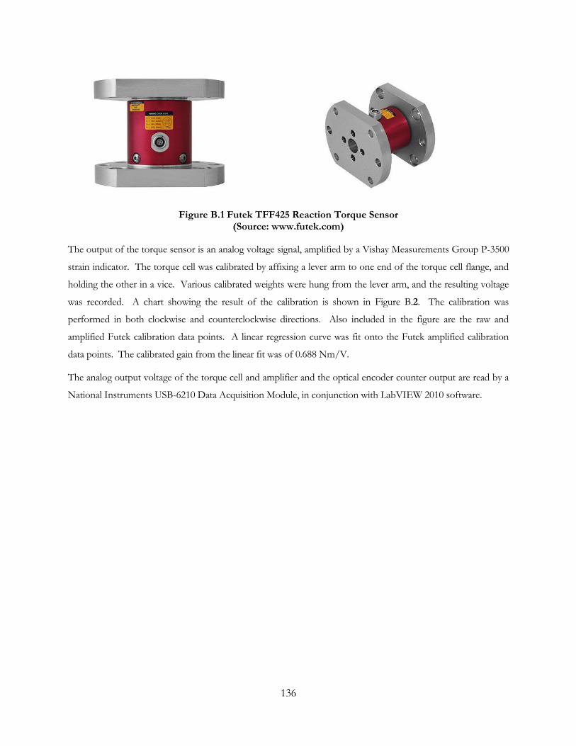
136
Figure B.1 Futek TFF425 Reaction Torque Sensor (Source: www.futek.com)
The output of the torque sensor is an analog voltage signal, amplified by a Vishay Measurements Group P-3500
strain indicator. The torque cell was calibrated by affixing a lever arm to one end of the torque cell flange, and
holding the other in a vice. Various calibrated weights were hung from the lever arm, and the resulting voltage
was recorded. A chart showing the result of the calibration is shown in Figure B.2. The calibration was
performed in both clockwise and counterclockwise directions. Also included in the figure are the raw and
amplified Futek calibration data points. A linear regression curve was fit onto the Futek amplified calibration
data points. The calibrated gain from the linear fit was of 0.688 Nm/V.
The analog output voltage of the torque cell and amplifier and the optical encoder counter output are read by a
National Instruments USB-6210 Data Acquisition Module, in conjunction with LabVIEW 2010 software.

137
Figure B.2 Torque Cell Calibration Curve
The torque cell has a low rating and is highly sensitive to fastener torque, wire orientation, and sensor
orientation. Therefore, torque sensor output was zeroed prior to beginning each test set to ensure accuracy.
The at-rest torque cell raw voltage was adjusted to offset the mean voltage reading of a 30-second test. This
offset was recorded and kept constant throughout the test set, or until the torque cell zero test was again
performed.
The particle brake is mounted vertically downward on the underside of the upper aluminum plate to transmit
torque directly from its housing to the plate and torque cell. The particle brake is connected to a 6.4 mm (1/4
inch) steel shaft via a flexible coupling.
An Encoder Products Company through-bore optical encoder with 500 pulse/revolution resolution and A-B
quadrature output with Z 0-degree referencing was used to measure turbine angular position and rotation rate.
The encoder contains a built-in sleeve bearing that accommodates a 6.4 mm diameter shaft. As the shaft and
bearing rotate, an internal optical sensor reads the pulses of the three A, B and Z output signals to determine
position and velocity. Due to the limitations of the data acquisition module, rpm and angular position could not
be measured simultaneously but instead were configured as desired prior to a particular test. A photo of the
optical encoder is shown in Figure B.3.
y = 0.688x - 3E-05R² = 1
-0.2
0
0.2
0.4
0.6
0.8
1
1.2
-0.2 0 0.2 0.4 0.6 0.8 1 1.2 1.4 1.6 1.8
Cal
ibra
ted
To
rque
, Nm
Amplifier Voltage Output, V
Clockwise Calibration
Counterclockwise Calibration
Futek Raw data
Futek Amplified Data
Linear (Futek Amplified Data)
138
Figure B.3 Optical Encoder
(Source: Encoder Products Company, 2011)
The A-B quadrature output determines the direction of rotation, in addition to measuring angular position or
rotational rate, and Z-referencing allows the encoder angle to reset after each revolution. When configured to
measure rpm, the encoder will only provide output data when the turbine is rotating. During each test set in
which angular position was being measured, the encoder begins the test with angle output set to zero, then as
the turbine begins rotation, the angular output resets to zero again when the Z-reference position is reached.
This requires post-processing of the results to correct angular position reading to an absolute azimuthal
reference frame.
The encoder requires a 5V input and digital ground signals. The encoder output is a set of digital voltage
counter signals, one each for A, B, and Z output. Three external pull-up resistors are required between each of
the outputs and 5V power.
The particle brake is a Placid Industries B2-12-1 magnetic particle brake with single shaft output and full torque
rating of 0.28 Nm. When current is applied to the particle brake via a power supply, magnetic particles within
the brake stator set up a magnetic field that opposes rotation of the brake rotor. The brake torque is roughly
proportional to the input current up to the rated torque of the device. There is some hysteresis in the curve,
depending whether current is being increased or decreased.
Although possible if carefully done, the particle brake calibration curve was not used to measure braking torque
via input current. Rather, the procedure for loading the turbine was to apply power to the particle brake and
adjust circuit resistance until the desired turbine rpm had been reached, then measure torque from the torque
cell.

139
In order to provide an adjustable load to the turbine, the particle brake current was varied by a rheostat and a
potentiometer in series with the particle brake/power supply circuit. The rheostat has a full resistance rating of
1000 ohm and was used for used as the coarse adjustment of resistance; the potentiometer rating was 100 ohms
and was used as the fine adjustment of resistance. The devices were fitted with knobs for manual adjustment
and were mounted to an electrical junction box. Both devices were of the “linear taper” type, meaning that
resistance is linear with angular position. Thus, the manual adjustment of the knobs had an inverse effect on
current and braking torque.
A photograph of the particle is shown in Figure B.4 (B2-24-1 is shown, which is similar to the B2-12-1 except
that it operates at 24 V).
Figure B.4 Particle Brake (Source: www.placidindustries.com)
Prior to static testing, the turbine position was correlated to the locking plate position and the locking plate was
locked into position on the rotating shaft. To lock the turbine into position, the turbine and locking plate were
rotated to the desired position, then a steel pin was inserted into the corresponding locking plate hole and
through the lower aluminum plate. This, along with setting the particle brake to full brake current, held the
turbine rigidly into a position during static testing.
A photograph of the instrumentation module as installed into the test flume is shown in Figure B.5.
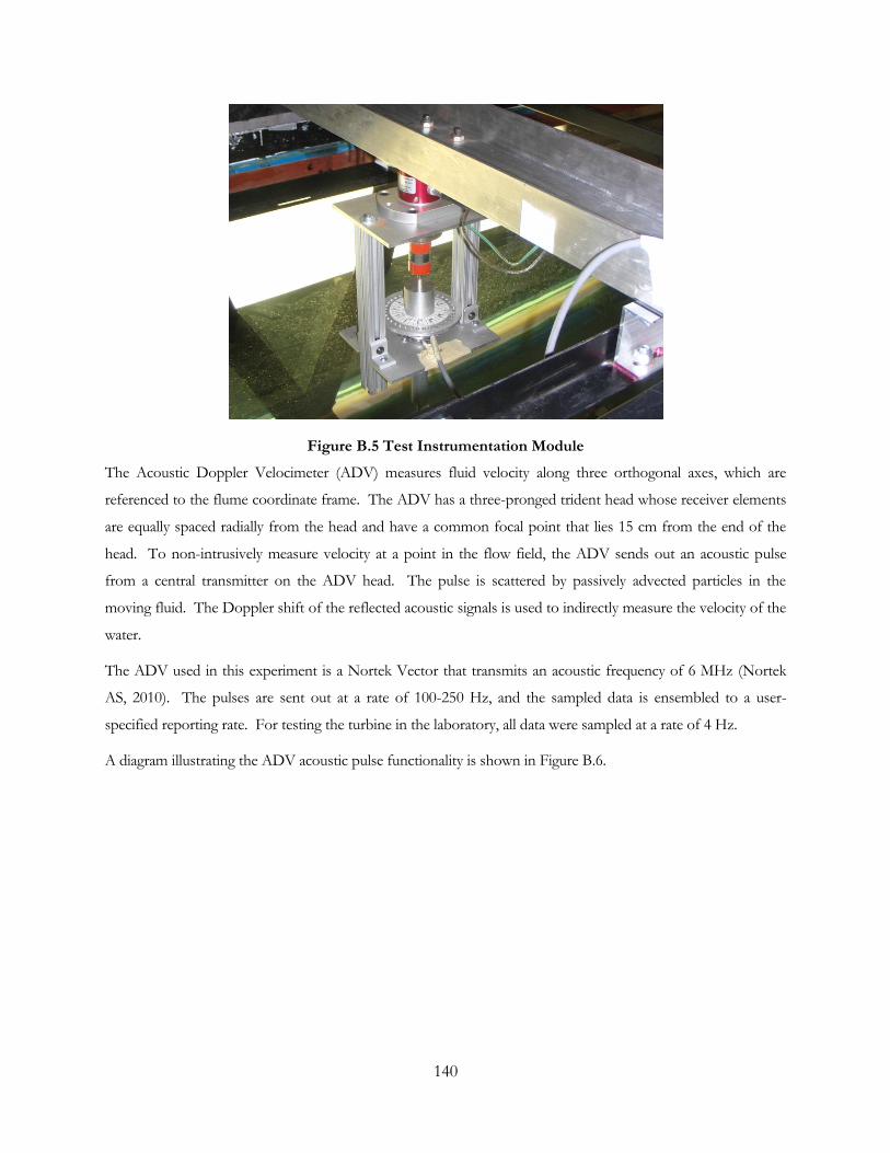
140
Figure B.5 Test Instrumentation Module
The Acoustic Doppler Velocimeter (ADV) measures fluid velocity along three orthogonal axes, which are
referenced to the flume coordinate frame. The ADV has a three-pronged trident head whose receiver elements
are equally spaced radially from the head and have a common focal point that lies 15 cm from the end of the
head. To non-intrusively measure velocity at a point in the flow field, the ADV sends out an acoustic pulse
from a central transmitter on the ADV head. The pulse is scattered by passively advected particles in the
moving fluid. The Doppler shift of the reflected acoustic signals is used to indirectly measure the velocity of the
water.
The ADV used in this experiment is a Nortek Vector that transmits an acoustic frequency of 6 MHz (Nortek
AS, 2010). The pulses are sent out at a rate of 100-250 Hz, and the sampled data is ensembled to a user-
specified reporting rate. For testing the turbine in the laboratory, all data were sampled at a rate of 4 Hz.
A diagram illustrating the ADV acoustic pulse functionality is shown in Figure B.6.

141
Figure B.6 ADV Illustration of Functionality (Source: Nortek AS, 2010)
A battery pack with embedded controller is connected to the ADV head and is used to process the data, which
is sent over a 3 analog channels on RS232 output. A RS232-to-USB analog-to-digital converter was used to
convert the signal. A laptop with Nortek proprietary software was used to receive, display and process the data
during testing.
The text files created by LabVIEW for the torque cell and encoder data consisted of the following:
1) Elapsed time (s)
2) Angular speed (rad/s)
3) Adjusted torque cell voltage (V)
4) Torque (Nm)
5) Rotation rate (RPM)
6) Unadjusted torque cell voltage (V)
7) Turbine angular reference position (degrees)
8) Turbine power (W)
9) Date and Time
10) Correlated ADV filename.
The ADV file set normally used for post-processing consisted of two synchronized files. One file contained the
synchronized data and time. The other file read the following data:
1) U velocity (in X-direction) (m/s)
2) V velocity (in Y-direction) (m/s)
3) W velocity (in Z-direction) (m/s).

142
This file also recorded signal amplitude, signal-to-noise ratio, and signal correlation, which were used to ensure
that the ADV was reading accurate data.

143
Appendix C: Additional Test Results and Tabular Data
This appendix provides additional data and selected test results in a tabular format.
Baseline Configuration
Table C.1 Baseline Configuration Load Performance Results
Table C.2 Static Torque Statistics for Baseline Configuration
Table C.3 Experimental Results of Tilted Turbine Test
Flume
velocity
(m/s)
Freewheel
Speed
Stall
Speed
Max
Torque
RPM at
Max
Torque Max CQ
RPM at
Max CQ
Max
Power
RPM at
Max
Power Max CP
RPM at
Max CP
0.80 201.4 119.6 0.159 119.6 0.143 119.6 2.17 142.1 0.209 142.1
0.77 190.3 112.9 0.146 112.9 0.142 112.9 1.86 129.8 0.200 129.8
0.70 160.8 95.7 0.101 95.7 0.119 95.7 1.09 118.1 0.158 118.1
0.60 131.0 86.6 0.060 86.6 0.096 86.6 0.55 91.1 0.126 91.1
0.50 100.9 65.2 0.034 65.2 0.080 65.2 0.23 65.2 0.095 65.2
0.40 62.5 50.5 0.017 50.5 0.061 50.5 0.09 50.5 0.069 50.5
Max Static Torque (Nm) 0.044
Max CQS 0.052
Angle of Max Torque 290
Min Static Torque (Nm) 0.012
Min CQS 0.015
Angle of Min Torque 160
Mean Static Torque (Nm) 0.034
Torque Std (Nm) 0.010
Connection
Design
Tilt Angle
(degrees)
Freewheel
Speed
Stall
Speed
Max
Torque
RPM at
Max
Torque Max CQ
RPM at
Max CQ
Max
Power
RPM at
Max
Power Max CP
RPM at
Max CP
% Power
Loss from
Zero Tilt
0 169.3 105.8 0.113 105.8 0.124 105.8 1.33 125.4 0.173 125.4 0%
2.5 166.0 101.4 0.114 101.4 0.122 101.4 1.29 121.0 0.163 121.0 -6%
5 164.0 101.0 0.109 101.0 0.116 101.0 1.25 116.0 0.158 119.7 -9%
10 156.7 102.6 0.096 102.6 0.100 102.6 1.08 115.0 0.133 115.0 -23%
0 177.1 103.1 0.119 103.1 0.131 103.1 1.45 124.1 0.191 124.1 0%
2.5 175.6 105.0 0.117 105.0 0.128 105.0 1.39 123.4 0.182 123.4 -4%
5 174.7 104.9 0.118 104.9 0.126 108.5 1.43 124.0 0.182 124.0 -4%
10 170.4 105.6 0.119 105.6 0.125 105.6 1.39 119.3 0.174 119.3 -9%
2 mm, 4-Leg
Spoke
2 mm
Circular
Plate

144
Table C.4 Performance Characteristics of 4-Bladed Turbine with Circular Plates
Wake Velocity Testing
The velocity data for the no load, maximum efficiency and static operating conditions is shown in Figure C.1
through Figure C.3 respectively. The data is plotted with error bars showing the standard deviation of the
velocity data. Mean velocity data is indicated by a square marker for tests with the turbine located at 70 cm from
the flume entrance and by a diamond marker for tests with the turbine located at 170 cm from the flume
entrance. At the two data points with identical relative stream-wise position (20 cm and 60 cm), the mean data
points lie within one standard deviation of each other.
The increased length of the error bars in the downstream wake for all three plots indicates increased turbulence
in the downstream wake.
Flume
velocity
(m/s)
Freewheel
Speed
Stall
Speed
Max
Torque
RPM at
Max
Torque Max CQ
RPM at
Max CQ
Max
Power
RPM at
Max
Power Max CP
RPM at
Max CP
0.80 214.1 117.7 0.173 117.7 0.155 117.7 2.48 145.4 0.240 150.3
0.70 167.5 101.2 0.102 101.2 0.122 101.2 1.19 123.2 0.177 123.2
0.60 132.9 80.0 0.060 83.3 0.096 83.3 0.55 99.3 0.127 99.3
0.50 100.9 63.7 0.034 65.5 0.078 65.5 0.23 65.5 0.092 65.5
0.40 64.4 51.4 0.016 51.4 0.057 51.4 0.09 51.4 0.067 51.4

145
Figure C.1 Centerline Mean Wake Velocity Data for Unloaded Turbine Diamond marker – turbine is at 170 cm position in flume. Square
marker - turbine is at 70 cm position in flume.
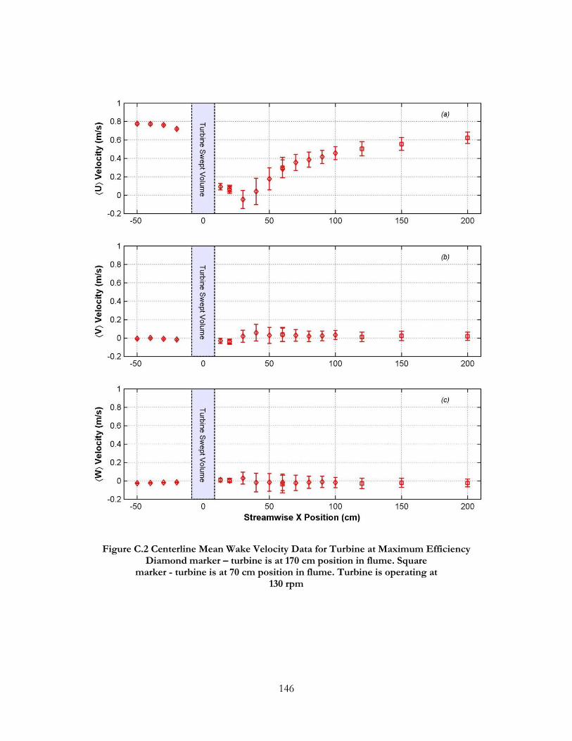
146
Figure C.2 Centerline Mean Wake Velocity Data for Turbine at Maximum Efficiency Diamond marker – turbine is at 170 cm position in flume. Square
marker - turbine is at 70 cm position in flume. Turbine is operating at 130 rpm

147
Figure C.3 Centerline Wake Velocity Data for Static Turbine Diamond marker – turbine is at 170 cm position in flume. Square
marker - turbine is at 70 cm position in flume.
Three-Bladed Turbine
The three bladed turbine was subjected to an operating performance test at several flume velocities and a static
torque test for its full revolution.

148
Table C.5 Performance Characteristics of 3-Bladed Turbine
Figure C.4 Load Performance Curves for 3-Bladed Turbine
Measurements of static torque were taken over the full revolution of the Three-Blade Turbine, at 10-degree
increments. Tests were conducted with a 6.4 mm central shaft and a three-leg spoke with thickness 4.8 mm.
Figure C.5 shows the static torque and static torque coefficient as a function of turbine angle for the Three-
Blade Turbine. Similar to the results of the Four-Blade Turbine, the static torque data points at each angle have
Flume
velocity
(m/s)
Freewheel
Speed
Stall
Speed
Max
Torque
RPM at
Max
Torque Max CQ
RPM at
Max CQ
Max
Power
RPM at
Max
Power Max CP
RPM at
Max CP
0.80 154.2 114.5 0.084 114.5 0.065 114.5 1.04 120.1 0.102 120.1
0.70 120.6 69.4 0.042 69.4 0.043 69.4 0.42 102.9 0.061 102.9
0.60 92.7 60.7 0.023 60.7 0.032 60.7 0.18 81.1 0.042 81.1
0.50 69.4 54.3 0.009 54.3 0.018 54.3 0.05 54.3 0.021 54.3

149
a high spread of data, as shown by the length of the standard deviation error bars. The static torque values, as
expected, exhibit a repeating pattern every 120°, corresponding to the blade sweep. Looking at reference Blade
End #1, whose leading edge starts at the 0 degree position, there are two maxima along the blade length: one
when the lower blade leading edge is at the 0 degree position, and another lower one when the lower blade
leading edge at 70 degrees. The minimum for the blade length occurs at 90-100 degrees. The mean static torque
for the turbine is shown as a dashed horizontal line.
Figure C.5 Static Torque of Three-Bladed Turbine
The tabular format of the data is shown in Table C.6.
Table C.6 Static Torque Statistics for Three-Bladed Turbine
Max Static Torque (Nm) 0.070
Max CQS 0.072
Angle of Max Torque 240
Min Static Torque (Nm) 0.019
Min CQS 0.019
Angle of Min Torque 90
Mean Static Torque (Nm) 0.044
Torque Standard Deviation (Nm) 0.013
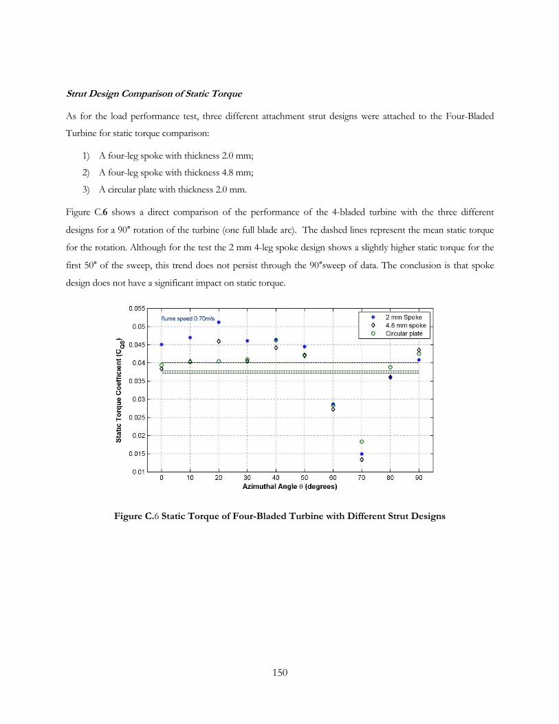
150
Strut Design Comparison of Static Torque
As for the load performance test, three different attachment strut designs were attached to the Four-Bladed
Turbine for static torque comparison:
1) A four-leg spoke with thickness 2.0 mm;
2) A four-leg spoke with thickness 4.8 mm;
3) A circular plate with thickness 2.0 mm.
Figure C.6 shows a direct comparison of the performance of the 4-bladed turbine with the three different
designs for a 90° rotation of the turbine (one full blade arc). The dashed lines represent the mean static torque
for the rotation. Although for the test the 2 mm 4-leg spoke design shows a slightly higher static torque for the
first 50° of the sweep, this trend does not persist through the 90°sweep of data. The conclusion is that spoke
design does not have a significant impact on static torque.
Figure C.6 Static Torque of Four-Bladed Turbine with Different Strut Designs

151
Appendix D: Blockage Analysis
If the turbine is modeled as a thin disc, and single streamtube theory is used to perform the analysis for
characterizing the flow, the entire channel may be modeled as shown in Figure D.1 (Polagye, 2009).
Figure D.1 Schematic of Single Streamtube Actuator Disc Theory for Turbine in a Channel Flow (Source: Polagye, 2009)
As shown in the figure there are three control volumes of interest:
Control Volume 1: Entire channel cross-section from far upstream of turbine to the end of wake expansion zone
Control Volume 2: Streamtube cross-section, representing only fluid that passes through the turbine actuator disc
model. This control volume extends from far upstream of the turbine to the end of the
wake expansion region. The cross-sectional area varies with the stream-wise direction.
Control Volume 3: Entire channel cross-section that encompasses the wake-mixing region
By applying the principles of conservation of mass, conservation of linear momentum, and conservation of
energy to the three control volumes, solution of each of the flow parameters is possible. Several such analyses
exist in the literature for estimating a correction factor for turbine performance in a blocked channel relative to a
large, open channel (Garrett & Cummins, 2007)(Bahaj, 2007)(Polagye, 2009)(Whelan, 2009). Two of these
analyses will be discussed here.
Garrett and Cummins (2007) derived a correction factor for a turbine operating at the maximum theoretical
limit is

152
. (D.1)
Here is the maximum turbine efficiency in partially blocked channel flow, is the maximum
efficiency in open channel flow and is the blockage ratio of the turbine in the channel.
This derivation made use of principles of conservation of mass and linear momentum but was based on the
assumption of a low Froude number and thus did not account for change to the channel water height resulting
from turbine power extraction and wake mixing. Their theory also assumes that the channel flow returns to its
original velocity at the end of the wake mixing region, such that u0=u5.
In his dissertation work, Polagye (2009) noted that Garrett and Cummins’ analysis, while providing an adequate
prediction for channel flow where turbine blockage ratio and Froude number are low, fails to address the
change in channel water height and thus violates conservation of mass. Polagye offered a similar analysis to
Garrett and Cummins but considered the change in channel height resulting from turbine power extraction and
wake mixing. The analysis again uses single streamtube theory, along with conservation of mass, linear
momentum and energy principles, to derive a set of equations for resolving flow rates in a partially blocked
channel. Referring to Figure D.1, the set of 3 equations to be solved are the following:
(D.2)
(D.3)
. (D.4)
In this set of equations, h0 refers to the water column height far upstream of the turbine and h3 refers to water
column height in the turbine wake at the end of the wake expansion region. The variable is a non-
dimensional parameter representing the ratio of wake velocity at the end of the expansion region u3 to
freestream velocity u0.
(D.5)
In the analysis Polagye determined that efficiency of power extraction and power dissipation is fundamentally a
function of three parameters: wake velocity ratio, Froude number, and blockage ratio.
(D.6)
Power extraction efficiency can also be represented in terms of α and control volume velocities:
(D.7)
153
The present analysis follows the work of Polagye to derive approximate bound to the correction factor of the
turbine efficiency for relating flume channel performance to performance in an open channel with the same
flow rate.
In the flume experiments, Fr and are known and are calculated from the following measured values: upstream
dynamic water height h0, the upstream velocity u0, and the turbine and flume cross-sectional areas.
By holding the flume speed constant and setting the velocity ratio as a variable parameter, three equations
(D.2), (D.3) and (D.4) were solved using a damped Newton numerical method. The power extraction
coefficient CP was then found using Equation (D.7). Several curves for as a function of were developed
that correspond to the operating conditions of data collected during flume testing. These curves are plotted in
Figure D.2. Assuming that the experimental data must coincide with the theoretical single streamtube solution,
the values for maximum power coefficient are overlain onto their respective curves. Additionally, data is plotted
for in open channel conditions, corresponding to Fr0 and 0.
The maximum possible coefficient of performance in open channel conditions approaches 0.59 for Fr0 and
0, which, as expected, coincides with the Lanchester-Betz limit for single streamtube theory. For the other
plots, as Fr and increase from 0, the maximum possible power coefficient increases from 0.59, as is
documented in the analyses by Garrett and Cummins and Polagye. For each case, is reached when the
wake velocity ratio is 0.33, consistent with Garrett and Cummins’ prediction of maximum efficiency of
extraction.
The plot is magnified in Figure D.2(b), showing more detail in the region of experimental data taken in the
Stevenson-Eroglu water flume for the baseline turbine configuration. Three experimental data conditions were
plotted onto the curves, each representing a case of maximum power for the turbine under the indicated
operating conditions. These conditions are shown in Table D.1.

154
Figure D.2 Schematic of Streamtube Theory Prediction of Power Coefficient
(a) Over entire range of α (b) Magnified in region of experimental data
Table D.1 Test Conditions for Blockage Ratio Calculations
It is expected that varies with loading. From the solution of the system of equations, it is possible to find a
correction factor to correct from of blocked conditions to of unblocked conditions over the entire
operating range of the turbine for a given Fr and .
(D.8)
0 0.2 0.4 0.6 0.8 10
0.1
0.2
0.3
0.4
0.5
0.6
0.7
0.8
0.9
1
aw
(a)
CP
0.88 0.9 0.92 0.94 0.96
0.15
0.16
0.17
0.18
0.19
0.2
0.21
0.22
aw
(b)C
P
Condition A
Condition B
Condition C
Unblocked Channel
Parameter Symbol
Test Condition -- A B C
Flume Speed (m/s) u0 0.7 0.7 0.8
Static Water Height hsw 50 47 46
Dynamic Water Height (cm) h0 47 44 42
Water Column Cross-Sectional Area (m2) AF 0.356 0.333 0.318
Turbine Cross-Sectional Area (m2) AC 0.040 0.040 0.040
Blockage Ratio ε 0.112 0.120 0.126
Froude Number Fr 0.326 0.337 0.394
Max Blade Reynold's Number (4-Bladed Turbine) ReB 8.0E+04 8.0E+04 9.5E+04
Min Blade Reynold's Number (4-Bladed Turbine) ReB 1.6E+04 1.6E+04 2.2E+04
Machine Reynold's Number (4-Bladed Turbine) ReM 1.4E+05 1.4E+05 1.5E+05
Flume Speed

155
Figure 4.14 shows the ratio plotted over the entire range of wake velocity ratio for each of the test
conditions.
Figure D.3 Power Coefficient Correction Factor as a Function of Wake Velocity Ratio
The drawback of the above method is that in order to provide a correction factor for a turbine in unblocked
conditions, it is necessary to know at least some part of the wake conditions: , , , , or , which are
difficult to define or measure in a physical sense. However, the curve for can be used to bound the correction
factor by using the values for at and .
The wake data experimental velocity ratio can be compared to the theoretical single streamtube wake velocity
ratio calculation to determine if the two values match. There is some uncertainty in performing this
comparison, as the theory does not provide for any analysis on the length of the wake expansion region and also
does not account for losses due to frame drag. Table D.2 shows the values from experimental results compared
to theoretical calculations of wake velocity ratio. The methodology presented above is used to back-calculate a
theoretical value for this power coefficient, assuming that and are uniquely related.The farthest
downstream velocity was taken as the u3 velocity for this comparison, as it provides results that are closest to
theoretical predictions. The results of the theoretical prediction versus estimation from experimental data differ
by around 12% but are comparable given the level of experimental uncertainty.
0 0.1 0.2 0.3 0.4 0.5 0.6 0.7 0.8 0.9 10.2
0.4
0.6
0.8
1
1.2
1.4
1.6
aw
Condition A
Condition B
Condition C
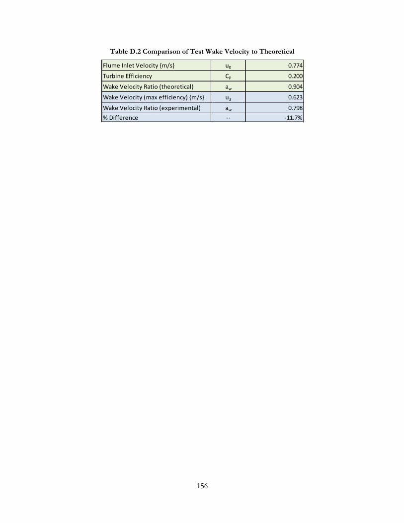
156
Table D.2 Comparison of Test Wake Velocity to Theoretical
Flume Inlet Velocity {m/s} u0 0.774
Turbine Efficiency CP 0.200
Wake Velocity Ratio (theoretical) aw 0.904
Wake Velocity (max efficiency) {m/s} u3 0.623
Wake Velocity Ratio (experimental) aw 0.798
% Difference -- -11.7%

157
Appendix E: Momentum Models
As a moving fluid passes through the swept area of a turbine, the turbine extracts energy from the fluid, causing
a momentum deficit (Burton et al., 2001). This is the basis for a momentum model analysis of a hydrokinetic
turbine. The turbine for a momentum model is modeled as a thin actuator disc or rectangular plate. A pressure
difference is established across the device, requiring the freestream velocity to decelerate across the “rotor” to
conserve mass and momentum. Behind the turbine, the streamtube and wake continue to expand until the
pressure in the wake equilibrates with freestream pressure (see Figure E.1 to follow). Far downstream of the
turbine, the wake and the freestream fluid continue to mix until the downstream velocity is once again uniform.
Blade element theory (as described in Section 3.1) is used to calculate forces on the blades using lift and drag
coefficients corresponding to the Reynolds number of the fluid and the angle of attack that the blade chord
makes with the relative fluid velocity.
Single Streamtube Model
A single streamtube model for a vertical axis turbine was first proposed by Templin (1974) for a Sandia
troposkein turbine. Templin’s model is based on actuator disc theory with a single, uniform, expanding
streamtube accounting for the momentum change across the turbine rotor. A diagram depicting a single
streamtube actuator disc for a hydrokinetic turbine is shown in Figure E.1. The curved, dashed lines represent
the boundaries of the streamtube. The subscripts “0” and “1” represent the freestream velocity far upstream of
turbine effects at stream-wise location “I”. The subscript “2” refers to values at the actuator disk. Subscript “3”
represents the wake zone following expansion of the wake region, but where the freestream velocity has not
mixed with the wake velocity. Subscript “4” is the freestream zone outside the wake at stream-wise location
“II”. Subscript “5” represents the region where wake and freestream have remixed to a uniform state far
downstream of the turbine at location “III”. The pressures “p+” and “p-“ refer to the fluid pressures just
upstream and just downstream of the turbine disc, respectively.
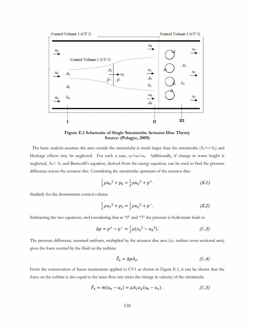
158
Figure E.1 Schematic of Single Streamtube Actuator Disc Theory Source: (Polagye, 2009)
The basic analysis assumes the area outside the streamtube is much larger than the streamtube (A1>>A0) and
blockage effects may be neglected. For such a case, u0=u4=u5. Additionally, if change in water height is
neglected, A0= A5 and Bernoulli’s equation, derived from the energy equation, can be used to find the pressure
difference across the actuator disc. Considering the streamtube upstream of the actuator disc:
. (E.1)
Similarly for the downstream control volume
. (E.2)
Subtracting the two equations, and considering that at “0” and “3” the pressure is hydrostatic leads to
. (E.3)
The pressure difference, assumed uniform, multiplied by the actuator disc area (i.e. turbine cross-sectional area)
gives the force exerted by the fluid on the turbine:
. (E.4)
From the conservation of linear momentum applied to CV1 as shown in Figure E.1, it can be shown that the
force on the turbine is also equal to the mass flow rate times the change in velocity of the streamtube
. (E.5)
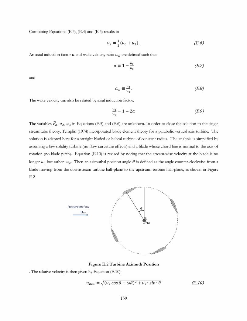
159
Combining Equations (E.3), (E.4) and (E.5) results in
. (E.6)
An axial induction factor and wake velocity ratio are defined such that
(E.7)
and
. (E.8)
The wake velocity can also be related by axial induction factor.
(E.9)
The variables , , in Equations (E.5) and (E.6) are unknown. In order to close the solution to the single
streamtube theory, Templin (1974) incorporated blade element theory for a parabolic vertical axis turbine. The
solution is adapted here for a straight-bladed or helical turbine of constant radius. The analysis is simplified by
assuming a low solidity turbine (no flow curvature effects) and a blade whose chord line is normal to the axis of
rotation (no blade pitch). Equation (E.10) is revised by noting that the stream-wise velocity at the blade is no
longer but rather . Then an azimuthal position angle is defined as the angle counter-clockwise from a
blade moving from the downstream turbine half-plane to the upstream turbine half-plane, as shown in Figure
E.2.
Figure E.2 Turbine Azimuth Position
. The relative velocity is then given by Equation (E.10).
(E.10)

160
The angle of attack for the simplified analysis is given by
. (E.11)
And the dynamic pressure q is given by
. (E.12)
The rest of the blade element analysis proceeds as in the blade element theory. To relate the axial force obtained
by momentum theory to force determined by blade element theory, the normal and tangential coefficients of a
small, differential blade element are resolved into components in the stream-wise direction.
(E.13)
The average axial force coefficient for a B-bladed turbine is found by integrating over the height of the turbine
and averaging over a revolution:
. (E.14)
Equating Equations (E.4) (streamtube momentum balance) and (E.14) for a given rotational speed and
freestream speed allows for a solution to be found for , , . Power and torque can then be calculated:
(E.15)
and
. (E.16)
Single streamtube theory provides a simple solution and works fairly well for lightly loaded turbines with low
solidity, but fails to provide an adequate prediction when more precise wind conditions are required, such as
wind shear effects (Strickland, 1975). Also, because the turbine is modeled as a thin disc, single streamtube
theory cannot resolve the effect of upstream blades on downstream blades.
Multiple Streamtube Model
A multiple streamtube model was originally proposed by Strickland (1975) to improve upon the accuracy of the
single streamtube model for vertical axis turbines, particularly to incorporate wind shear variation and provide a
more accurate distribution of blade forces.
Multiple streamtube theory incorporates the same momentum and blade element principles as single streamtube
theory. The major difference is that the single streamtube is divided into several streamtubes that form a 2-D
grid spatially in the plane perpendicular to the stream-wise direction. This gives rise to a velocity distribution in
the 2-D plane, allowing incorporation of ground shear effects and resolution of individual axial force
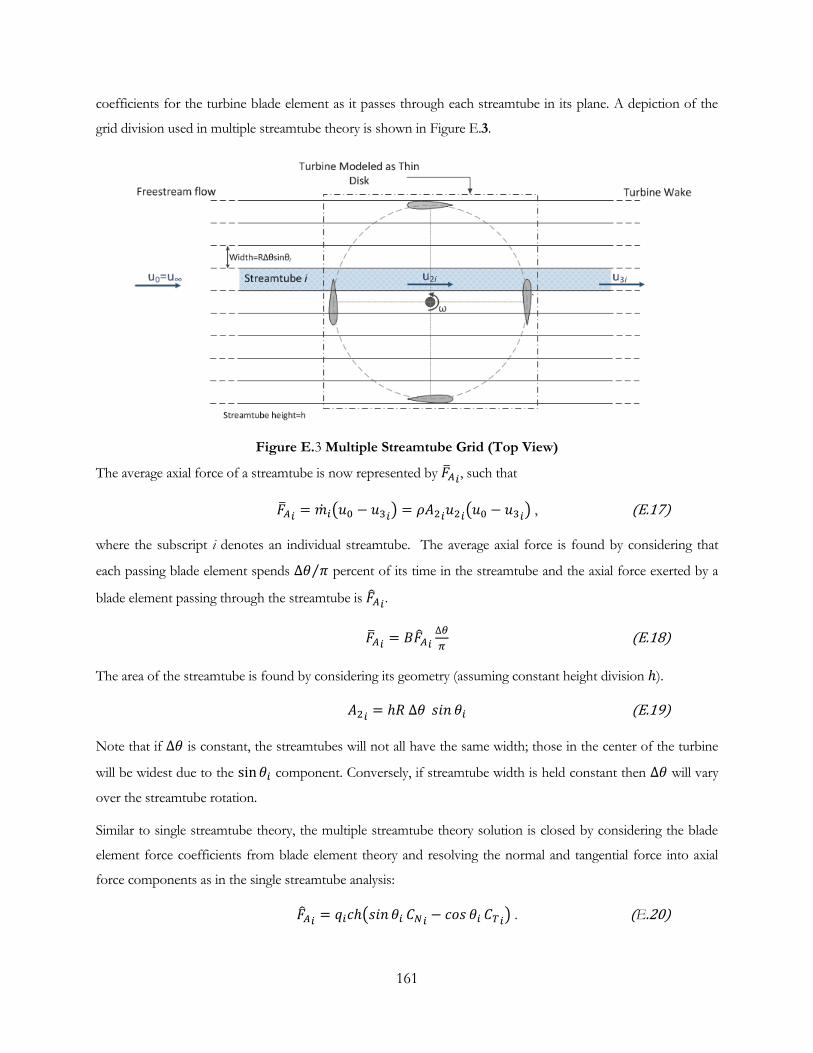
161
coefficients for the turbine blade element as it passes through each streamtube in its plane. A depiction of the
grid division used in multiple streamtube theory is shown in Figure E.3.
Figure E.3 Multiple Streamtube Grid (Top View)
The average axial force of a streamtube is now represented by , such that
, (E.17)
where the subscript i denotes an individual streamtube. The average axial force is found by considering that
each passing blade element spends percent of its time in the streamtube and the axial force exerted by a
blade element passing through the streamtube is .
(E.18)
The area of the streamtube is found by considering its geometry (assuming constant height division ).
(E.19)
Note that if is constant, the streamtubes will not all have the same width; those in the center of the turbine
will be widest due to the component. Conversely, if streamtube width is held constant then will vary
over the streamtube rotation.
Similar to single streamtube theory, the multiple streamtube theory solution is closed by considering the blade
element force coefficients from blade element theory and resolving the normal and tangential force into axial
force components as in the single streamtube analysis:
. (E.20)

162
Once the solution is found and , , are resolved for each streamtube, the total blade force, torque, and
power are determined by considering the tangential force component and by summing the contributions of each
blade element to obtain a single blade torque. Then the blade torque is found for each position by time-
averaging over the full revolution (or in other words, streamtube averaging over the streamtubes in a half-
revolution for a particular blade). For torque this is given by
. (E.21)
Here B is the number of blades, is the number of time increments, and is a blade segment tangential
force, which is summed over the length of a single blade.
Multiple streamtube theory was shown by Strickland (1975) to improve turbine prediction from single
streamtube theory (due to its ability to provide an improved force resolution and incorporation of shear effects).
However, this theory still cannot predict any wake effects on downstream blades from an upstream passing
blade. Additionally, the multiple streamtube method does not differentiate between the performance of a helical
turbine and a straight-bladed Darrieus turbine, since the spatial average of the two turbines is identical, unless a
yawing correction factor is introduced that accounts for any performance degradation due to the stream-wise
velocity vector impacting the turbine blade at an angle not equal to 90 degrees.
Double Multiple Streamtube Model
Double multiple streamtube theory builds upon multiple streamtube theory by considering that the upstream
pass of blades in a vertical axis turbine reduces the velocity and affects the performance of blades in the
downstream pass (Paraschivoiu, 1988). The analysis is similar to multiple streamtube theory, except that
streamtubes are divided into an upstream half-rotor and downstream-half rotor with each half being considered
separately. Two actuator discs are used to approximate the turbine, one on the upstream blade pass and the
other on the downstream blade pass. An equilibrium velocity is assumed to exist between the two actuator
discs, the value of which is determined by analysis of the upstream disc, and which is used as the stream-wise
velocity input of the downstream disc. Figure E.4 provides a schematic showing streamtubes for double
multiple streamtube theory.

163
Figure E.4 Double Multiple Streamtube Grid (Top View)
The analysis of the upstream disc proceeds as for the multiple streamtube analysis, the only difference being that
each blade spends now only percent of its time in the streamtube. The average force of the upstream
streamtube is given by
, (E.22)
where the subscripts “A” from multiple streamtube analysis have been replaced by “U” to note that this is an
analysis of the upstream rotor. Additionally, the wake velocity from multiple streamtube theory is replaced
by the equilibrium velocity between the actuator discs for the upstream analysis. The force
is calculated
as in Equation (E.20) for multiple streamtube analysis. The momentum Equations (E.5) and (E.6) are revised
giving
(E.23)
and
. (E.24)
The rest of the analysis of the upstream rotor pass proceeds as in multiple streamtube theory, solving for ,
, and
for each streamtube. Considering the tangential force component and summing the individual
streamtube contributions results in force, torque and power values for the upstream half-rotor pass only.
The downstream pass analysis is similar, only the input velocity values have changed. The stream-wise velocity
is now and the downstream wake velocity is now
. Average blade element force for the streamtube is

164
found from Equation (E.25) where the downstream axial force is obtained from modifying Equation
(E.20).
(E.25)
As the fluid passes through the downstream half-rotor, energy is assumed to be extracted for the streamtube as
in momentum theory of the single streamtube analysis (that is to say, is treated as the undisturbed
freestream velocity). The resulting downstream disc velocity given by
. (E.26)
And the downstream axial force from momentum theory is given by
(E.27)
The unknowns for the downstream pass are now , , and which are solved in the same methods as
for the upstream analysis. Summing each individual streamtube and considering the tangential force
contribution gives the force, torque, and power for the downstream pass only. The average for a total revolution
requires averaging the upstream and downstream half-rotors results. For torque this is given by
(E.28)
Double multiple streamtube analysis was shown by Paraschivoiu (1988) to give more accurate results compared
to experimental data than multiple streamtube analysis for a vertical axis turbine with low solidity and high tip
speed ratio. Paraschiviou (1988) noted that at low tip speed ratio the model performance is degraded by its
inability to account for dynamic stall (see Section 3.5.2). As for any streamtube model, no differentiation is
possible between helical and straight-bladed Darrieus turbine.
All multiple streamtube models suffer from the inability to predict non-stream-wise velocity components.
Additionally, model accuracy is poor in the near wake (within 1-2 diameters of the rotor) (Strickland et al., 1979).
However, these techniques are much less computationally intensive than vortex or CFD models.

165
Appendix F: Cascade Model Methodology
The cascade model is based on cascade theory for turbo-machinery by Hirsch & Mandal (1987) and was
summarized for a straight vertical axis turbine by Dai et al. (2011). According to Hirsch & Mandal, the cascade
model overcomes the inaccuracy at high tip speed ratio and higher solidity that reduces the effectiveness of
double multiple streamtube models. This is done by including an empirical correction for induced velocity as a
function of solidity ratio, and calculating the influence of a reference blade on the pressure and velocity of the
other blades. The following derivation below follows the method of Dai et al. (2011) for a vertical axis turbine.
The cascade model translates the circular path traced out by the blades into a straight path, as shown in Figure
F.1. The distance between blade quarter chord points is given by the arc length:
. (F.1)
One of the blades is assumed to be the reference blade (e.g., blade labeled “1” in Figure F.1 and its path is traced
for one full revolution in increments of .
Figure F.1 Cascade Model Path Transformation
(Source: Dai et al., 2011)
The cascade model analysis is similar to double multiple streamtube theory. The rotor is split into several
streamtubes and, for each streamtube, an angle of attack and relative velocity are based on an initial estimate of
. The elemental lift and drag forces are then calculated for each streamtube for the upstream pass:
(F.2)
and

166
. (F.3)
In the linear cascade transformation as shown in Figure F.1, each turbine blade is assumed to see the same
relative velocity. The model makes a correction for the local velocity on the forward and aft blades (e.g., blades
“2” and “3” due to the influence of the reference blade. First the blade “1” circulation is calculated from
. (F.4)
Then a velocity correction due to the circulation effects on the other two nearest blades is found by
. (F.5)
The relative velocities and angle of attack of the other blades are then corrected in the tangential direction (y-
direction as shown in Figure F.1).
(F.6)
(F.7)
(F.8)
(F.9)
The pressure difference before and after the cascade is then found by
. (F10)
The local equilibrium velocity is found as
. (F.11)
From here an experimental fit is used to find the induced upstream velocity . A coefficient k is found by
experimental fit (Hirsch & Mandal, 1987) to be
(F.12)
This constant is used to calculate the induced velocity:
(F.13)

167
The value for is found by averaging the value from Equation (F.13) for each streamtube. The solution for
the induced velocity is iterated until it converges on a solution. The solution method by Dai differs from
previously presented double multiple streamtube analysis in that a single induced velocity is determined for the
entire upstream pass.
The downstream pass of the rotor analysis proceeds after the upstream analysis as in the double multiple
streamtube model, with replacing , replacing
, and replacing . After both upstream and
downstream solutions are found, the total torque and power for revolution is found by averaging streamtube
results for each respective half-revolution and then adding the results of upstream and downstream passes.
The cascade model incorporates a correction for turbine solidity and blade interactions, giving the modeling
method an advantage over streamtube models and the vortex models, both of which fail to account for solidity
in effects in determining performance, other than by chord length. The cascade model was shown by Hirsch &
Mandal (1987) to provide good comparison to experimental results for a turbine with solidity ratio 0.13
compared to results predicted by double multiple stream tube theory. However, no comparison to results with
solidity ratios higher than 0.13 were presented. When flow curvature effects were added to streamtube
theory, the models were of roughly equal validity. One drawback of the cascade model method is that it fails to
provide guidance for determining the solution for a turbine with greater than three blades.