www.CalSolarResearch.ca.gov

Final Project Report:

Advanced Modeling and

Verification for High

Penetration PV

Grantee:

Clean Power Research

April 2012

California Solar Initiative

Research, Development, Demonstration

and Deployment Program RD&D:

PREPARED BY

10 Glen Ct. Napa, CA 94558 707-224-9992

Principal Investigator: Tom E. Hoff TomHoff@CleanPower.com

Project Partners: State University of New York National Renewable Energy Laboratory New York State Energy Research and Development Authority Solar Electric Power Association Sacramento Municipal Utility District Salt River Project Long Island Power Authority New York Power Authority

PREPARED FOR

California Public Utilities Commission California Solar Initiative: Research, Development, Demonstration, and Deployment Program

CSI RD&D PROGRAM MANAGER

Program Manager: Ann Peterson Ann.Peterson@itron.com

Project Manager: Smita Gupta Smita.Gupta@itron.com

Additional information and links to project related documents can be found at http://www.calsolarresearch.ca.gov/Funded-Projects/

DISCLAIMER

“Any opinions, findings, and conclusions or recommendations expressed in this material are those of the author(s) and do not necessarily reflect the views of the CPUC, Itron, Inc. or the CSI RD&D Program.”

Preface

The goal of the California Solar Initiative (CSI) Research, Development, Demonstration, and Deployment (RD&D) Program is to foster a sustainable and self-supporting customer-sited solar market. To achieve this, the California Legislature authorized the California Public Utilities Commission (CPUC) to allocate $50 million of the CSI budget to an RD&D program. Strategically, the RD&D program seeks to leverage cost-sharing funds from other state, federal and private research entities, and targets activities across these four stages:

Grid integration, storage, and metering: 50-65%

Production technologies: 10-25%

Business development and deployment: 10-20%

Integration of energy efficiency, demand response, and storage with photovoltaics (PV)

There are seven key principles that guide the CSI RD&D Program:

1. Improve the economics of solar technologies by reducing technology costs and increasing system performance;

2. Focus on issues that directly benefit California, and that may not be funded by others;

3. Fill knowledge gaps to enable successful, wide-scale deployment of solar distributed generation technologies;

4. Overcome significant barriers to technology adoption;

5. Take advantage of California’s wealth of data from past, current, and future installations to fulfill the above;

6. Provide bridge funding to help promising solar technologies transition from a pre-commercial state to full commercial viability; and

7. Support efforts to address the integration of distributed solar power into the grid in order to maximize its value to California ratepayers.

For more information about the CSI RD&D Program, please visit the program web site at www.calsolarresearch.ca.gov.

2

Acknowledgements This project was a success as a result of the contributions of people at a wide variety of organizations. The California Public Utilities Commission (CPUC), Pacific Gas and Electric Company (PG&E), San Diego Gas and Electric Company (SDG&E), Southern California Edison (SCE), and New York State Energy Research and Development Authority (NYSERDA) provided financial support. Smita Gupta (Itron) managed the grant in such a way so as to result in a usable set of products, and Ann Peterson (Itron) provided support. Obadiah Barthomy (SMUD), Matt Heling (PG&E), and Jim Blatchford (California ISO) provided valuable direction and support from the municipal utility, investor owned utility, and independent system operator perspectives. Mike Taylor (SEPA) was effective at disseminating information. Personnel at ConEd and PG&E, and Jeff Peterson and Jacques Roeth (NYSERDA) provided valuable feedback and direction on the PV value tool.

A4 Ranch and the City of Napa provided land access to run a data collection effort that provided crucial data for the project. Richard Perez produced a prolific amount of new research and led the SUNY research lab to develop a new solar resource model. Ben Norris (CPR) designed an innovative, low-cost method to collect solar resource data, lead the implementation of the Grid Services and PV Value Analysis Tool, and provided valuable review. Phil Gruenhagen (CPR) implemented the Grid Services and PV Value Tool. David Chalmers (CPR) mastered the challenges associated with producing a solar resource database that was 200 times the resolution of the standard resolution database. Jan Kleissl (UC San Diego) performed valuable research that assessed the performance of SolarAnywhere and provided obstruction profiles to integrate into SolarAnywhere. Kelly Folly (Vote Solar) brought research results into CPUC’s LTPP.

Thanks to all of these individuals and organizations, as well as many others, for their support and assistance.

3

Contents Acknowledgements ....................................................................................................................................... 2

Abstract ......................................................................................................................................................... 6

Executive Summary ....................................................................................................................................... 7

Introduction .............................................................................................................................................. 7

Project Objectives ..................................................................................................................................... 7

Results ....................................................................................................................................................... 7

Solar Resource Data .............................................................................................................................. 7

Analysis of Geographically Dispersed PV Systems ................................................................................ 8

Methodology to Simulate High Speed PV Fleet Output ....................................................................... 8

Distributed PV Value Analysis Tool ....................................................................................................... 8

List of Accomplishments ........................................................................................................................... 8

Pending Patents .................................................................................................................................... 8

Journal Articles ...................................................................................................................................... 9

Conference Presentations ..................................................................................................................... 9

Webinars ............................................................................................................................................... 9

Solar Data ............................................................................................................................................ 10

Recommendations .................................................................................................................................. 10

Introduction ................................................................................................................................................ 11

Project Objectives ....................................................................................................................................... 11

Project Approach and Outcomes ................................................................................................................ 12

Task 1: Technology Transfer and Outreach ............................................................................................ 12

Journal Articles .................................................................................................................................... 12

Conference Presentations ................................................................................................................... 12

Webinars ............................................................................................................................................. 13

Task 2: Improved Solar Radiation Datasets ............................................................................................ 13

Background ......................................................................................................................................... 13

Objective ............................................................................................................................................. 13

Approach ............................................................................................................................................. 13

Results ................................................................................................................................................. 14

Task 3: PV Output Variability .................................................................................................................. 18

Background ......................................................................................................................................... 18

4

Objective ............................................................................................................................................. 18

Approach ............................................................................................................................................. 18

Results ................................................................................................................................................. 19

Task 4: High Penetration PV T&D Model Integration ............................................................................. 23

Objective ............................................................................................................................................. 23

Approach ............................................................................................................................................. 23

Results ................................................................................................................................................. 23

Task 5: Optimal PV Location Identification ............................................................................................. 25

Background ......................................................................................................................................... 25

Objective ............................................................................................................................................. 25

Approach ............................................................................................................................................. 25

Results ................................................................................................................................................. 26

Conclusions ................................................................................................................................................. 28

Recommendations ...................................................................................................................................... 29

Public Benefits to California ........................................................................................................................ 30

Solar Resource Data ................................................................................................................................ 30

Analysis of Geographically Dispersed PV Systems .................................................................................. 30

Methodology to Simulate High-Speed PV Fleet Output ......................................................................... 30

Distributed PV Value Analysis Tool ......................................................................................................... 31

Appendix A: Grid Software Services ........................................................................................................... 32

Overview ................................................................................................................................................. 32

PV Systems and Fleet Definitions............................................................................................................ 32

Software Service Parameters .................................................................................................................. 34

Software Services – Administrative (Summary)...................................................................................... 35

Software Service Descriptions ................................................................................................................ 36

Appendix B: Optimal PV Location Identification Tool Description ............................................................. 39

Background ............................................................................................................................................. 39

Introduction ............................................................................................................................................ 40

Objective ............................................................................................................................................. 41

Overview ............................................................................................................................................. 41

Units of Results ................................................................................................................................... 41

PV Production And Loss Savings ............................................................................................................. 43

5

PV System Output ............................................................................................................................... 43

Loss Savings ......................................................................................................................................... 45

Value Component Methodology ............................................................................................................. 47

Energy Value ....................................................................................................................................... 47

Generation Capacity Value ..................................................................................................................... 48

Environmental Value ........................................................................................................................... 49

Fuel Price Hedge Value ....................................................................................................................... 50

T&D Capacity Value ............................................................................................................................. 51

Total Value .......................................................................................................................................... 52

References .............................................................................................................................................. 53

6

Abstract The California Solar Initiative (CSI) has a goal of installing 3,000 MW of new solar electricity by 2016. CSI has identified PV grid integration with regard to the planning and modeling for high-penetration PV as one potential barrier to accomplishing this goal. A team led by Clean Power Research (CPR) received approval from the California Public Utilities (CPUC) for a grant titled, “Advanced Modeling and Verification for High Penetration PV.”

The CPR-led team designed a project to address the issue of high-penetration PV according to the following four tasks:

1. Enhance spatial and temporal resolution of solar radiation data sets for California. 2. Enhance and validate PV modeling tools to include output variability. 3. Integrate PV modeling capabilities into a distribution system engineering and analysis tools. 4. Create a tool to calculate economic value of a specific PV fleet configuration, whether it be

distributed or central station.

These tasks have been accomplished and are discussed in this report. In order to make the results as accessible as possible, they have also been documented in three patent applications, six peer reviewed journal articles, seven conference papers, three webinars, and a state-of-the art solar resource database for all of California (www.solaranywhere.com).

7

Executive Summary

Introduction The California Solar Initiative (CSI) has a goal of installing 3,000 MW of new solar electricity by 2016. One of the components needed to accomplish this goal is to address key market barriers to installing increasing volumes of solar distributed generation. CSI has identified the issue of PV grid integration with regard to the planning and modeling for high-penetration PV as one potential barrier.

Clean Power Research (CPR) received grant approval from the California Public Utilities (CPUC) for a grant titled, “Advanced Modeling and Verification for High Penetration PV.” A grant agreement was signed with Itron, the Program Manager, on April 2, 2010.

CPR assembled a team to address this issue that includes solar radiation experts (State University of New York), a government lab (National Renewable Energy Laboratory), a state energy organization (New York State Energy Research and Development Authority), an industry trade group (Solar Electric Power Association), and several utilities (Sacramento Municipal Utility District, Salt River Project, Long Island Power Authority, and New York Power Authority).

Project Objectives The team designed a project to address the issue of high-penetration PV according to the following four tasks.

1. Enhance spatial and temporal resolution of solar radiation datasets for selected California locations.

2. Enhance and validate PV modeling tools to include output variability. 3. Integrate PV modeling capabilities into distribution system engineering and analysis tools. 4. Create a tool to calculate the economic value of a specific PV fleet configuration, whether it be

distributed or central station.

Results The tasks were completed and have provided a number of benefits to the state of California.

Solar Resource Data The enhanced spatial and temporal resolution solar radiation data set was developed not just for selected locations, but for the entire state of California. It is referred to as SolarAnywhere Enhanced Resolution and is publicly available at www.solaranywhere.com. This state-of-the-art database provides the highest known resolution of any satellite-based irradiance data set in the world, with a 1 km x 1 km spatial resolution and a half-hour temporal resolution. This data set has a number of benefits.

• The California ISO used the solar resource data as input into the high penetration PV analysis documented in the “Summary of Preliminary Results of 33% Renewable Integration Study.”

• UCSD has used the data set to both validate its accuracy and perform a variety of research projects.

• A variety of users have downloaded the data for their analysis.

8

Analysis of Geographically Dispersed PV Systems The team performed a significant amount of research in studying the effect of geographically dispersed PV systems on output variability. A key finding was that output variability reduces as PV systems are more geographically dispersed. This research has been beneficial to a number of utilities in California and has helped to begin to allay some of the concerns associated with this variability. It has also highlighted the conditions under which such variability has the potential to occur: in situations where PV is highly concentrated in one location (i.e., large, single PV facilities or highly concentrated PV on a distribution system). This will have planning benefits at both the transmission and distribution levels.

Methodology to Simulate High Speed PV Fleet Output One of the significant research finds from this project was a novel methodology to simulate the power output of any PV fleet over any high speed time interval. This new methodology has multiple benefits.

• It represents a significant step forward in helping utilities and the California lSO have a method to perform grid integration studies.

• It holds much promise when applied to short-term output variability used to forecast PV system performance.

• The result was patented and CPUC was named a party to the patent.

Distributed PV Value Analysis Tool A tool was developed under this grant agreement to assist in the economic evaluation of distributed PV systems. The overall objective of this project is to incorporate PV value analysis methodologies into a software service that equips users with the ability to perform such studies independently. The resulting software service will calculate the location-specific economic value of distributed PV generation from the perspective of the utility. The following value components will be included in the analysis: energy value, generation capacity value, environmental value, fuel price hedge value, T&D capacity value, and loss savings. The tool greatly simplifies the approach of calculating the economic value of PV. It has been made available to a variety of stakeholders in California with a particular focus on utility planners.

List of Accomplishments A substantial amount of work was accomplished under the grant agreement. In order to make the results as accessible as possible, the results are listed here. The results were documented in three patent applications, six peer reviewed journal articles, seven conference papers, three webinars, and a state-of-the art solar resource database for all of California.

Pending Patents 1. Computer-Implemented System and Method for Estimating Power Data for a Photovoltaic Power

Generation Fleet. 2. Computer-Implemented System and Method for Determining Point-to-Point Correlation of Sky Clearness

for Photovoltaic Power Generation Fleet Output Estimation. 3. Computer-Implemented System and Method for Efficiently Performing Area-to-Point Conversion of

Satellite Imagery for Photovoltaic Power Generation Fleet Output Estimation.

9

Journal Articles 1. “Quantifying PV Power Output Variability,” Solar Energy, Volume 84, Issue 10, October 2010, Pages 1782-

1793. http://www.sciencedirect.com/science/article/pii/S0038092X10002380. 2. “Modeling PV Fleet Output Variability,” Solar Energy, December 2011 (Electronic Version), Print version

forthcoming. Draft available at http://www.cleanpower.com/Content/Documents/research/capacityvaluation/Modeling%20PV%20Fleet%20Output%20Variability.pdf.

3. “Parameterization of Site-specific Short-term Irradiance Variability,” Solar Energy, Volume 85, Issue 7, July 2011, Pages 1343-1353, http://www.sciencedirect.com/science/article/pii/S0038092X11000995.

4. “Short-term Solar Irradiance Variability – Spatial and Temporal Characteristics”, Solar Energy, Submitted. Draft available at http://www.cleanpower.com/Content/Documents/research/capacityvaluation/Short-term%20irradiance%20variability%20-%20Station%20pair%20correlation%20as%20a%20function%20of%20distance.pdf.

5. “Solar Resource Variability: Myth and Fact,” Solar Today, August/September 2011. http://www.solartoday-digital.org/solartoday/20110910#pg48.

6. “Solar Power Generation in the US: Too Expensive or a Bargain?” Accepted to Energy Policy, Forthcoming. Draft available at http://www.cleanpower.com/Content/Documents/research/capacityvaluation/Solar%20Power%20Generation%20in%20the%20US%20-%20Too%20Expensive%20or%20a%20Bargain.pdf.

Conference Presentations 1. “Short-Term Irradiance Variability: Station Pair Correlation as a Function of Distance,” ASES National

Conference, Raleigh, NC, 2011. Draft available at http://www.asrc.cestm.albany.edu/perez/2011/short.pdf.

2. “PV Power Output Variability: Calculation of Correlation Coefficients Using Satellite Insolation Data,” ASES National Conference, Raleigh, NC, 2011. Draft available at http://www.cleanpower.com/Content/Documents/research/capacityvaluation/SOLAR2011_36.pdf.

3. “High Solar Penetration: Challenges on Day-Ahead and Multi-Day Forecasts,” AMS Summer Community Meeting, August 2011.

4. “The Convergence of Distributed PV, Smart Grid & Storage,” SEPA Utility Solar Conference, August 2011, Available at http://sepa.confex.com/sepa/2011usc/webprogram/Session1092.html.

5. “Meeting Intermittency Challenges Using Simulated PV Fleet Production,” Solar Power International 2011, Dallas, Texas.

6. “Determining Storage Reserves for Regulating Solar Variability,” Electrical Energy Storage Applications and Technologies 2011, San Diego, California. Available at http://www.cleanpower.com/Content/Documents/research/capacityvaluation/EESAT%20Paper%20-%20Norris%2011-07-2011.pdf.

7. “Solar Resource Assessment Workshop (太阳能资源评估 研讨会)”, Dezhou, Shandong province, China, Dec. 10, 2011.

Webinars 1. PV output variability, the sheep in wolf’s clothing,” VoteSolar, March 2011. Recording available at

http://votesolar.org/tag/solar-output/. 2. Solar PV Variability and Distribution Feeder Performance, EPRI, March 2011 3. Solar Forecasting: Modeling, Verification and High Penetration PV, SEPA, August 2011. Recording available

at http://www.solarelectricpower.org/resources/multimedia-library.aspx?kw=sepa%20seminar.

10

Solar Data 1. Provided detailed data to CAISO for inclusion in 33% renewables case study. Summary of Preliminary

Results of 33% Renewable Integration Study – 2010 CPUC LTPP Docket No. R.10-05-006. Report available at http://www.cpuc.ca.gov/NR/rdonlyres/E2FBD08E-727B-4E84-BD98-7561A5D45743/0/LTPP_33pct_initial_results_042911_final.pdf. Page 87.

2. Partial validation of SolarAnywhere 2009 by UCSD. Available at http://www1.eere.energy.gov/solar/pdfs/highpen2wkshp_05intro_jkleissl_forecasting_110613.pdf, page 10.

3. SolarAnywhere Enhanced Resolution (1 km x 1 km, half-hour) freely available to general public at www.solaranywhere.com.

Recommendations There are several next steps that have been identified for this work. They include:

1. Create a high resolution solar resource database (spatial resolution of 1 km x 1 km, temporal resolution of one-minute) to forecast PV fleet performance.

2. Validate the PV fleet simulation methodology. 3. Integrate the PV fleet simulation methodology powered by the high resolution solar resource

database into utility software tools. 4. Transfer the fleet simulation technology to California utilities and balancing area authorities.

11

Introduction The California Solar Initiative (CSI) has a goal of installing 3,000 MW of new solar electricity by 2016. One of the activities needed to accomplish this goal is to address key market barriers to installing increasing volumes of solar distributed generation. CSI has identified the issue of PV grid integration with regard to the planning and modeling for high-penetration PV as one potential barrier.

Clean Power Research (CPR) received grant approval from the California Public Utilities (CPUC) for a grant titled, “Advanced Modeling and Verification for High Penetration PV.” A grant agreement was signed with Itron, the Program Manager, on April 2, 2010.

CPR assembled a team to address this issue that includes solar radiation experts (State University of New York), a government lab (National Renewable Energy Laboratory), a state energy organization (New York State Energy Research and Development Authority), an industry trade group (Solar Electric Power Association), and several utilities (Sacramento Municipal Utility District, Salt River Project, Long Island Power Authority, and New York Power Authority).

Project Objectives The CPR-led team designed a project to address the issue of high-penetration PV according to the following four tasks.

1. Enhance spatial and temporal resolution of solar radiation data sets for selected California locations.

2. Enhance and validate PV modeling tools to include output variability. 3. Integrate PV modeling capabilities into distribution system engineering and analysis tools. 4. Create a tool to calculate the economic value of a specific PV fleet configuration, whether it be

distributed or central station.

The objective of the project was to accomplish these four tasks.

12

Project Approach and Outcomes This section describes the approaches used to accomplish each of the tasks and outcomes.

Task 1: Technology Transfer and Outreach The first task was project management and technology transfer. The following journal articles, conference proceedings, and webinars were completed.

Journal Articles 1. “Quantifying PV Power Output Variability,” Solar Energy, Volume 84, Issue 10, October 2010, Pages 1782-

1793. http://www.sciencedirect.com/science/article/pii/S0038092X10002380. 2. “Modeling PV Fleet Output Variability,” Solar Energy, December 2011 (Electronic Version), Print version

forthcoming. Draft available at http://www.cleanpower.com/Content/Documents/research/capacityvaluation/Modeling%20PV%20Fleet%20Output%20Variability.pdf.

3. “Parameterization of Site-specific Short-term Irradiance Variability,” Solar Energy, Volume 85, Issue 7, July 2011, Pages 1343-1353, http://www.sciencedirect.com/science/article/pii/S0038092X11000995.

4. “Short-term Solar Irradiance Variability – Spatial and Temporal Characteristics,” Solar Energy, Submitted. Draft available at http://www.cleanpower.com/Content/Documents/research/capacityvaluation/Short-term%20irradiance%20variability%20-%20Station%20pair%20correlation%20as%20a%20function%20of%20distance.pdf.

5. “Solar Resource Variability: Myth and Fact,” Solar Today, August/September 2011. http://www.solartoday-digital.org/solartoday/20110910#pg48.

6. “Solar Power Generation in the US: Too Expensive or a Bargain?” Accepted to Energy Policy, Forthcoming. Draft available at http://www.cleanpower.com/Content/Documents/research/capacityvaluation/Solar%20Power%20Generation%20in%20the%20US%20-%20Too%20Expensive%20or%20a%20Bargain.pdf.

Conference Presentations 1. “Short-Term Irradiance Variability: Station Pair Correlation as a Function of Distance,” ASES National

Conference, Raleigh, NC, 2011. Draft available at http://www.asrc.cestm.albany.edu/perez/2011/short.pdf.

2. “PV Power Output Variability: Calculation of Correlation Coefficients Using Satellite Insolation Data,” ASES National Conference, Raleigh, NC, 2011. Draft available at http://www.cleanpower.com/Content/Documents/research/capacityvaluation/SOLAR2011_36.pdf.

3. “High Solar Penetration: Challenges on Day-Ahead and Multi-Day Forecasts,” AMS Summer Community Meeting, August 2011.

4. “The Convergence of Distributed PV, Smart Grid & Storage,” SEPA Utility Solar Conference, August 2011, Available at http://sepa.confex.com/sepa/2011usc/webprogram/Session1092.html.

5. “Meeting Intermittency Challenges Using Simulated PV Fleet Production,” Solar Power International 2011, Dallas, Texas.

6. “Determining Storage Reserves for Regulating Solar Variability,” Electrical Energy Storage Applications and Technologies 2011, San Diego, California. Available at http://www.cleanpower.com/Content/Documents/research/capacityvaluation/EESAT%20Paper%20-%20Norris%2011-07-2011.pdf.

13

7. “Solar Resource Assessment Workshop (太阳能资源评估 研讨会),” Dezhou, Shandong province, China, Dec. 10, 2011.

Webinars 1. PV output variability, the sheep in wolf’s clothing,” VoteSolar, March 2011. Recording available at

http://votesolar.org/tag/solar-output/. 2. Solar PV Variability and Distribution Feeder Performance, EPRI, March 2011 3. Solar Forecasting: Modeling, Verification and High Penetration PV, SEPA, August 2011. Recording available

at http://www.solarelectricpower.org/resources/multimedia-library.aspx?kw=sepa%20seminar.

Task 2: Improved Solar Radiation Datasets The second task was to enhance the spatial and temporal resolution of solar radiation data sets for selected California locations.

Background SolarAnywhere® is an online satellite-based irradiance dataset (www.SolarAnywhere.com) currently available in the continental U.S. and Hawaii. It is a subscription-based service that contains hourly irradiance data at a 10 km by 10 km spatial resolution dating back from 1998 to a 7-day ahead forecast.

Objective Under this grant, the functionality of SolarAnywhere was extended in three ways:

1. Finer spatial resolution ( 1 km by 1 km grid). 2. Finer temporal resolution (30 min interval). 3. Freely available to users throughout California for the term of the grant project.

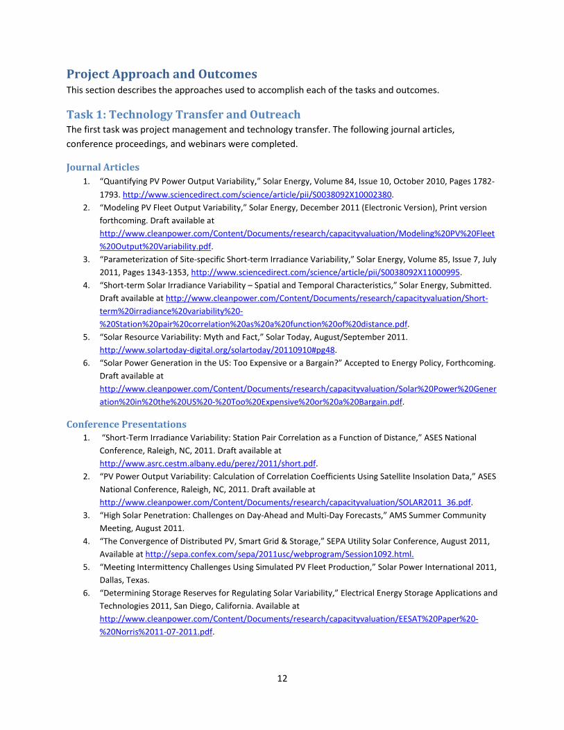
Approach As illustrated in Figure 1, the new SolarAnywhere Enhanced Resolution data set represents a 200-fold increase in the amount of data when compared to the existing SolarAnywhere Standard Resolution data set. The bottom part of the figure illustrates the difference in data resolution for a single location (San Francisco, CA).

The approach to producing this data was to obtain access to higher spatial and temporal resolution satellite imagery than what was used in SolarAnywhere Standard Resolution, and to upgrade server capabilities to host the data. Due to the amount of data, the original proposal was to produce the data for a limited number of regions in California.

14

Figure 1. Enhanced spatial and temporal resolution data set results in 200-fold increase in data.

San Francisco, CA

Results The original task in the grant agreement was to produce SolarAnywhere Enhanced Resolution data in areas where the CSI program has already experienced high PV penetration. The team decided to exceed the terms of the grant agreement and produce Enhanced Resolution data for every location in California.

This task was completed and SolarAnywhere Enhanced Resolution data (1 km x 1 km spatial resolution and half-hour temporal resolution) was made publicly available for the entire state of California. These data have been regularly updated and are available free of charge. Data can be downloaded at www.SolarAnywhere.com.

15

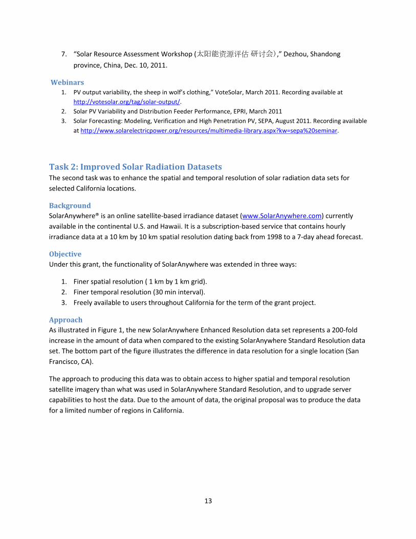
Figure 2. Publicly available solar resource data (available at www.SolarAnywere.com).

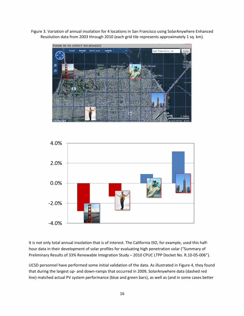
There has been strong interest in this data as it can be used in a variety of ways. At the most basic level, the data can be used to optimize plant location. For example, CPR recently participated at a solar resource assessment workshop in China.1 One of the topics at the workshop was how to optimally site the large scale PV systems that are planned for China. CPR used the SolarAnywhere Enhanced Resolution data to illustrate how to site plants to optimize for performance. As illustrated in Figure 3, CPR illustrated how the annual solar insolation varied by +/- 3 percent within a distance of less than 10 km. Chinese investors were interested in how such an approach could be applied for China.

1 Solar Resource Assessment workshop, Dezhou, Shandong province, China, Dec. 9-11, 2011.

16

Figure 3. Variation of annual insolation for 4 locations in San Francisco using SolarAnywhere Enhanced Resolution data from 2003 through 2010 (each grid tile represents approximately 1 sq. km).

It is not only total annual insolation that is of interest. The California ISO, for example, used this half-hour data in their development of solar profiles for evaluating high penetration solar (“Summary of Preliminary Results of 33% Renewable Integration Study – 2010 CPUC LTPP Docket No. R.10-05-006”).

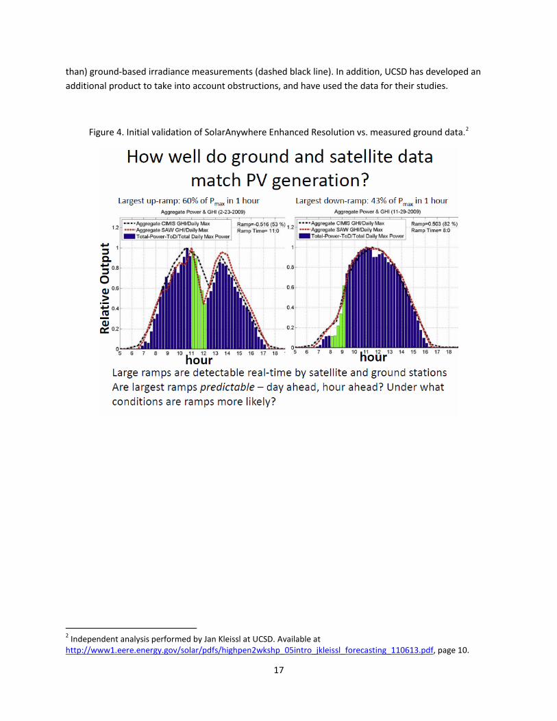
UCSD personnel have performed some initial validation of the data. As illustrated in Figure 4, they found that during the largest up- and down-ramps that occurred in 2009, SolarAnywhere data (dashed red line) matched actual PV system performance (blue and green bars), as well as (and in some cases better

17

than) ground-based irradiance measurements (dashed black line). In addition, UCSD has developed an additional product to take into account obstructions, and have used the data for their studies.

Figure 4. Initial validation of SolarAnywhere Enhanced Resolution vs. measured ground data.2

2 Independent analysis performed by Jan Kleissl at UCSD. Available at http://www1.eere.energy.gov/solar/pdfs/highpen2wkshp_05intro_jkleissl_forecasting_110613.pdf, page 10.

18

Task 3: PV Output Variability The third task was to enhance and validate PV modeling tools to include output variability.

Background PV capacity is increasing on utility systems. As a result, utility planners and grid operators are growing more concerned about potential impacts of power supply variability caused by transient clouds. Utilities and control system operators need to adapt their planning, scheduling, and operating strategies to accommodate this variability while at the same time maintaining existing standards of reliability.

It is impossible to effectively manage these systems, however, without a clear understanding of PV output variability or the methods to quantify it. Whether forecasting loads and scheduling capacity several hours ahead, or planning for reserve resources years into the future, the industry needs to be able to quantify expected output variability for fleets of up to hundreds of thousands of PV systems spread across large geographical territories. Underestimating reserve requirements may result in a failure to meet reliability standards and an unstable power system. Overestimating reserve requirements may result in an unnecessary expenditure of capital and higher operating costs.

Objective The purpose of this task was to develop and test output variability algorithms that could then be used to perform PV simulations on a sub-hourly time scale. Variability in time intervals ranging from a few seconds to a few minutes is of primary interest since control area reserves are dispatched over these time intervals.

The original plan was that the validation would be performed using high-speed, measured, PV fleet data provided by the utility partners. Once the project was initiated, however, it was determined that none of the utility partners had the required data. For this reason, the scope was modified to validate irradiance data based on measured data obtained from a CPR-installed irradiance network.

Approach CPR previously developed a method to estimate the output variability associated with a fleet of identically sized and spaced PV systems. The original approach to accomplish the objective was to extend the output variability algorithms to cover arbitrary system configurations, and to test using measured high speed PV system output data from a fleet of PV systems from several utilities.

Both an issue and an opportunity arose that resulted in modifying the original approach. The issue was that measured high speed PV output data from a fleet of PV systems located close together was unavailable from any of the utility partners involved in the project. The opportunity was that, while the focus was on determining how to estimate output variability (i.e., the rate of change in output), the research resulted in a significant find that facilitated the modeling of both output variability and the more fundamental quantity of output.

In terms of the issue, an alternative to high speed, centralized PV system monitoring was developed to provide a means for collecting the required variability data. Temporary, small-scale irradiance measurement stations were constructed and then deployed to mimic the behavior of larger PV systems,

19

thus avoiding the costs and complexities of central monitoring. This approach provided sufficient accuracy and temporal resolution to determine changes in system output. They were then deployed in two different test regimens.

In terms of the opportunity, during the course of research, it appeared that CPR’s original research could be extended to include both output variability and output. As a result, the effort expended on this task (Task 3) was increased to fully develop the model and the effort on the next task (Task 4) was reduced.

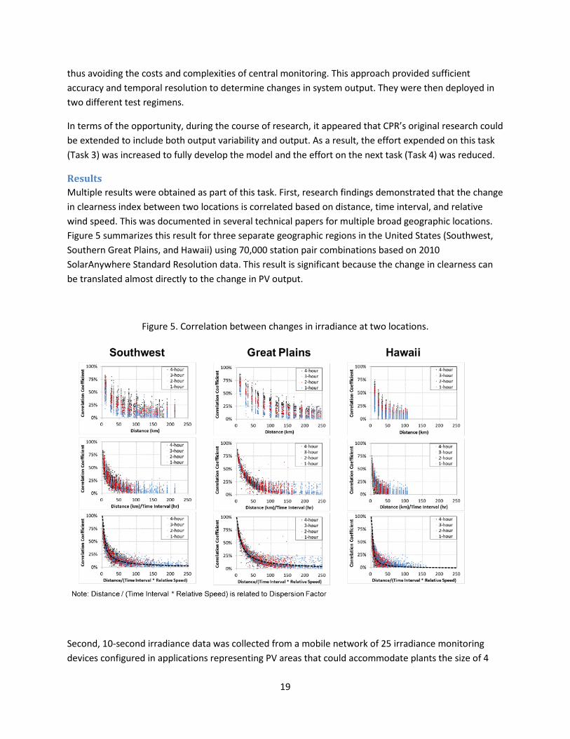
Results Multiple results were obtained as part of this task. First, research findings demonstrated that the change in clearness index between two locations is correlated based on distance, time interval, and relative wind speed. This was documented in several technical papers for multiple broad geographic locations. Figure 5 summarizes this result for three separate geographic regions in the United States (Southwest, Southern Great Plains, and Hawaii) using 70,000 station pair combinations based on 2010 SolarAnywhere Standard Resolution data. This result is significant because the change in clearness can be translated almost directly to the change in PV output.

Figure 5. Correlation between changes in irradiance at two locations.

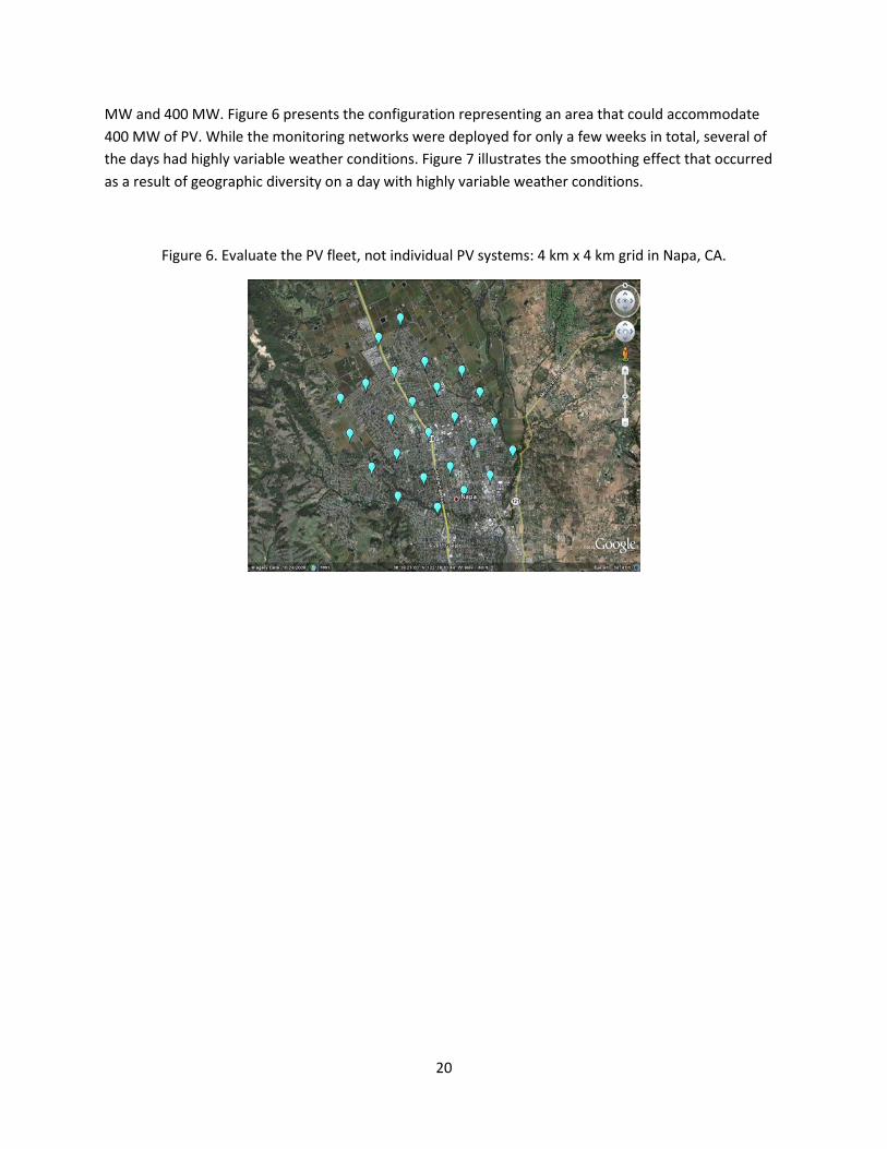
Second, 10-second irradiance data was collected from a mobile network of 25 irradiance monitoring devices configured in applications representing PV areas that could accommodate plants the size of 4

20

MW and 400 MW. Figure 6 presents the configuration representing an area that could accommodate 400 MW of PV. While the monitoring networks were deployed for only a few weeks in total, several of the days had highly variable weather conditions. Figure 7 illustrates the smoothing effect that occurred as a result of geographic diversity on a day with highly variable weather conditions.

Figure 6. Evaluate the PV fleet, not individual PV systems: 4 km x 4 km grid in Napa, CA.

21

Figure 7. Measured 10-second irradiance data from 4 km x 4 km grid in Napa on highly variable weather day (Nov. 21, 2010).

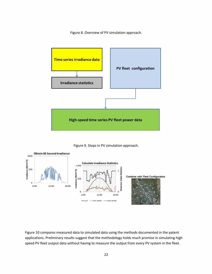
Third, these results were combined together in a method to simulate high speed PV fleet output for any arbitrary PV fleet configuration. Figure 8 presents an overview of how the approach works, and Figure 9 illustrates the steps using measured data. Together, these results culminated in the filing of three patent applications:

1. Computer-Implemented System and Method for Estimating Power Data for a Photovoltaic Power Generation Fleet.

2. Computer-Implemented System and Method for Determining Point-to-Point Correlation of Sky Clearness for Photovoltaic Power Generation Fleet Output Estimation.

3. Computer-Implemented System and Method for Efficiently Performing Area-to-Point Conversion of Satellite Imagery for Photovoltaic Power Generation Fleet Output Estimation.

22

Figure 8. Overview of PV simulation approach.

Figure 9. Steps in PV simulation approach.

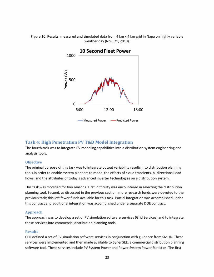
Figure 10 compares measured data to simulated data using the methods documented in the patent applications. Preliminary results suggest that the methodology holds much promise in simulating high speed PV fleet output data without having to measure the output from every PV system in the fleet.

23

Figure 10. Results: measured and simulated data from 4 km x 4 km grid in Napa on highly variable weather day (Nov. 21, 2010).

Task 4: High Penetration PV T&D Model Integration The fourth task was to integrate PV modeling capabilities into a distribution system engineering and analysis tools.

Objective The original purpose of this task was to integrate output variability results into distribution planning tools in order to enable system planners to model the effects of cloud transients, bi-directional load flows, and the attributes of today’s advanced inverter technologies on a distribution system.

This task was modified for two reasons. First, difficulty was encountered in selecting the distribution planning tool. Second, as discussed in the previous section, more research funds were devoted to the previous task; this left fewer funds available for this task. Partial integration was accomplished under this contract and additional integration was accomplished under a separate DOE contract.

Approach The approach was to develop a set of PV simulation software services (Grid Services) and to integrate these services into commercial distribution planning tools.

Results CPR defined a set of PV simulation software services in conjunction with guidance from SMUD. These services were implemented and then made available to SynerGEE, a commercial distribution planning software tool. These services include PV System Power and Power System Power Statistics. The first

24

service can be used to assist in fault location identification and evaluating the effect of load transfers. The second service can be used for PV interconnection studies and utility system design. A third service will be developed to simulate fleet power. It can be used for ISO regulation and load serving entity scheduling.

The Grid Services are described in detail in the Appendix.

25

Task 5: Optimal PV Location Identification The fifth task was to create a tool to calculate economic value of a specific PV fleet configuration, whether it be distributed or central station.

Background There is an inherent tension between the value of power and the cost of power. The value of power is highest for on-site generation while the cost of power is lowest for off-site generation. This is because the value of power increases while the cost of power decreases with proximity to consumption. Power value increases near the point of consumption because delivery costs are reduced and other benefits are realized. Power cost decreases away from the point of consumption because generation is located far away from at least some loads due to the economies of scale associated with most types of generation.

PV, however, is one technology that helps to resolve this tension because it disobeys the economies of scale rule. PV is only mildly influenced by the size of the generating facility because the fundamental building block in a PV power generation system, the PV module, is the same whether it is used in a small PV system located at an individual’s house, or a very large PV plant located in the desert. This, along with other attributes associated with distributed PV generation has captured people’s attention for more than two decades.

While there is substantial interest in distributed generation, utility planners currently lack the tools necessary to quickly and easily quantify the value of distributed PV based on when, where, what type, and how much PV is installed. The lack of tools is a result of several practical challenges in performing a distributed PV value analyses. One challenge is that an accurate evaluation requires time series PV output data specific to the location being evaluated. The PV modeling to produce the required data requires solar resource datasets, which, until recently, have been difficult to obtain. Another challenge is that the nature of the value components requires expertise from several different disciplines including distribution planning, generation planning, regional renewable energy markets, and engineering economics.

Objective The purpose of this task is to produce a tool to identify optimal PV location based on the technical and economic value of distributed PV. This tool could then be used by distribution planners to quickly assess the value of distributed PV, or by policy makers to assist in the design of a value-based feed-in-tariff (FIT).

Approach CPR has developed and applied analytical methodologies for calculating the value of distributed PV power generation for more than 20 years. The company has performed such studies from as far back as analysis of the first installed distributed PV plant at PG&E’s Kerman substation in the early 1990s, to more recent studies.

A three-step approach was taken to develop the tool. First, the methodologies were summarized in a report. Second, a draft Excel spreadsheet was developed. Third, a web-based tool was developed. The

26

value components including in the analysis are: loss savings, energy, generation capacity, fuel price hedge, T&D capacity, and environmental.

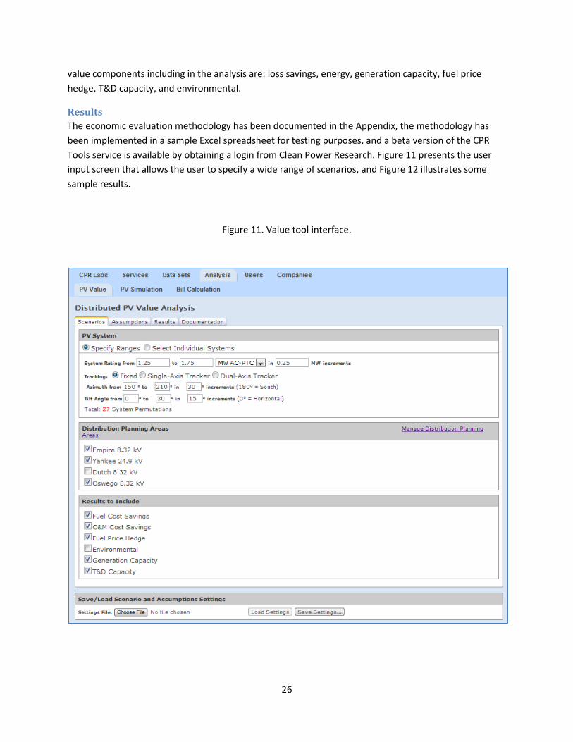
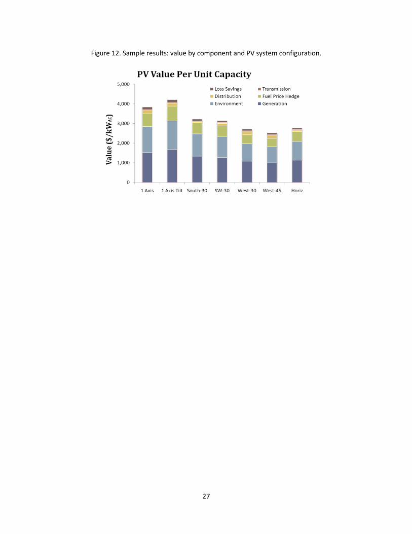
Results The economic evaluation methodology has been documented in the Appendix, the methodology has been implemented in a sample Excel spreadsheet for testing purposes, and a beta version of the CPR Tools service is available by obtaining a login from Clean Power Research. Figure 11 presents the user input screen that allows the user to specify a wide range of scenarios, and Figure 12 illustrates some sample results.

Figure 11. Value tool interface.

27

Figure 12. Sample results: value by component and PV system configuration.

28

Conclusions The California Solar Initiative (CSI) has a goal of installing 3,000 MW of new solar electricity by 2016. One requirement for accomplishing this goal is to address key market barriers to installing increasing volumes of solar distributed generation. CSI has identified the issue of PV grid integration with regard to the planning and modeling for high-penetration PV as one potential barrier.

The objective of this grant was to address the issue of high-penetration PV by accomplishing four tasks. The four tasks were:

1. Enhance spatial and temporal resolution of solar radiation data sets for selected California locations.

2. Enhance and validate PV modeling tools to include output variability. 3. Integrate the PV modeling capabilities into distribution system engineering and analysis tools. 4. Create a tool to calculate the economic value of a specific PV fleet configuration, whether it be

distributed or central station.

The deliverables for the first, second, and fourth tasks were met and exceeded. Progress was made toward accomplishing the third task and further extended under a separate DOE contract; further work still remains.

For the first task, enhanced resolution solar resource data was developed for the entire State of California rather than just for selected locations. For the second task, not only was a model developed for output variability, the model was extended to include the more fundamental variable of output. When combined, the results from Task 1 and Task 2 lay the foundation necessary to simulate time series PV fleet output for any arbitrary fleet at any time increment. For the fourth task, the deliverable of an Excel spreadsheet was completed, and further progress was made with the implementation of a draft version of the web-based software tool.

Thus, overall, the results from this grant should be deemed quite successful. Three of the four tasks were exceeded, and results were documented in three patent applications, six peer reviewed journal articles, seven conference papers, and three webinars. California has free access to a state-of-the-art enhanced resolution solar resource database for the entire state.

29

Recommendations There are several next steps that have been identified for this work. They include:

1. Create a high resolution solar resource database (spatial resolution of 1 km x 1 km, temporal resolution of one-minute) to forecast PV fleet performance.

2. Validate the PV fleet simulation methodology. 3. Integrate the PV fleet simulation methodology powered by the high resolution solar resource

database into utility software tools. 4. Transfer the fleet simulation technology to California utilities and balancing area authorities.

30

Public Benefits to California This project has provided a number of benefits to the state of California.

Solar Resource Data SolarAnywhere Enhanced Resolution is a state-of-the-art database. It provides the highest known resolution of any satellite-based irradiance data set in the world (1 km x 1 km spatial resolution with half-hour temporal resolution). This data set has a number of benefits.

• It is freely available for California. • The California ISO used the solar resource data as input into the high penetration PV analysis

documented in the “Summary of Preliminary Results of 33% Renewable Integration Study.” • UCSD has used the data set to both validate its accuracy as well as to perform a variety of

research projects. • A variety of unidentified users have downloaded the data for their analysis.

In addition, SolarAnywhere Enhanced Resolution has the potential to be extended to other countries. China is implementing many GW of large-scale PV plants and has become interested in using high resolution data to help optimally site PV plants. This could translate into increased tax revenue to the state of California if CPR can financially capitalize on this interest, as CPR is headquartered in California as pays California taxes.

Analysis of Geographically Dispersed PV Systems The CPR-led team performed a significant amount of research in studying the effect geographically dispersed PV systems have on output variability. The key finding was that more geographically dispersed PV systems have less correlated output, and thus less output variability. This result was illustrated in Figure 7.

This research has been beneficial to a number of utilities in California, helping to allay some of the concerns associated with this variability. It has also highlighted the conditions under which such variability has the potential to occur: in situations where PV is highly concentrated in one location (i.e., large, single PV facilities or highly concentrated PV on a distribution system). This will have planning benefits at both the transmission and distribution levels.

Methodology to Simulate High-Speed PV Fleet Output One of the significant research finds from this project was a novel methodology to simulate the power output of any PV fleet over any high-speed time interval. This new methodology has multiple benefits.

• It represents a significant step forward for utilities and the California lSO by providing a method to perform grid integration studies.

• It holds much promise as applied to short-term output variability used to forecast PV system performance.

• The result was patented and CPUC was named a party to the patent.

31

Distributed PV Value Analysis Tool A tool was developed under this grant agreement to assist in the economic evaluation of distributed PV systems. The overall objective of this project is to incorporate PV value analysis methodologies into a software service that equips users with the ability to perform such studies independently. The resulting software service will calculate the location-specific economic value of distributed PV generation from the perspective of the utility. The following value components will be included in the analysis: energy value, generation capacity value, environmental value, fuel price hedge value, T&D capacity value, and loss savings.

The tool greatly simplifies the approach of calculation the economic value of PV. It has been available to a variety of stakeholders in California with a particular focus on utility planners. It also has the potential to be useful to policy makers in designing a value-based feed-in-tariff (FIT).

32

Appendix A: Grid Software Services

Overview This appendix describes a set of software services that relate to modeling fleets of PV systems on the distribution and transmission grids. These services are available to support the planning and operation of a wide variety of utility, power market, and regulation functions.

PV Systems and Fleet Definitions PV Systems in CPR software services are currently defined by a set of object classes that describe performance attributes used by PVSimulator (module efficiency, temperature coefficients, inverter efficiency, etc.), as well as shading, orientation, and lat/long location. To provide grid simulations, these classes had to be expanded to include additional attributes.

Each PV system is now described by the following:

• CPR PV “Energy System” Object • Grid Status (Online, Offline, Proposed) • ISO/RTO Control Area ID (e.g., CAISO, New England ISO) • Control Area Participant3 (e.g., PG&E, SMUD, Blythe Energy LLC)

Every PV system has the potential to be associated with an ISO/RTO Control Area, and all PV systems in this control area effectively define a “top level” fleet. For example, fleet variability may be calculated for the aggregate set of PV systems in a control area.

Control Area Participants include Load Serving Entities, such as utilities, and these Participants may correspond to a user/subscriber. For example, PG&E could be a user of the service in order to develop daily “net” load forecasts for submission to the CAISO. Control Area Participants may be individual power producers on a state transmission network.

Each user is able to define and modify its own set of fleets according to the type of study desired. For example, PG&E might want to know variability on a particular feeder or on all feeders connected to a common substation bus. These fleet definitions may be thus defined in different hierarchical levels (utility, region, substation, feeder, subfeeder) and may overlap.

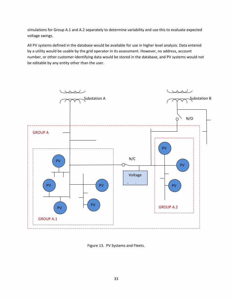
For example, in Figure 13, the fleet defined by Group A might be defined by all PV systems connected to Substation A at a given time. This fleet could be defined to forecast PV output during the time of the peak summer load or to detect fault location using the expected output from each PV system at the time of the fault. Group A.2 could be defined for a different purpose. For example, if the voltage regulator shown is being operated too frequently due to high cloud variability, the utility may want to determine the impacts of shifting loads to Substation B. Before performing this operation, the utility could run

3 Participants can be traditional vertically integrated investor-owned utilities, municipal utilities, load-serving entities that own little or no generation, or independent power producers.

33

simulations for Group A.1 and A.2 separately to determine variability and use this to evaluate expected voltage swings.

All PV systems defined in the database would be available for use in higher level analysis. Data entered by a utility would be usable by the grid operator in its assessment. However, no address, account number, or other customer-identifying data would be stored in the database, and PV systems would not be editable by any entity other than the user.

Figure 13. PV Systems and Fleets.

Substation A Substation B

N/C

PV

PV PV

PV

PV

N/O

PV

PV

PV

GROUP A

GROUP A.1

GROUP A.2

Voltage

R l t

34

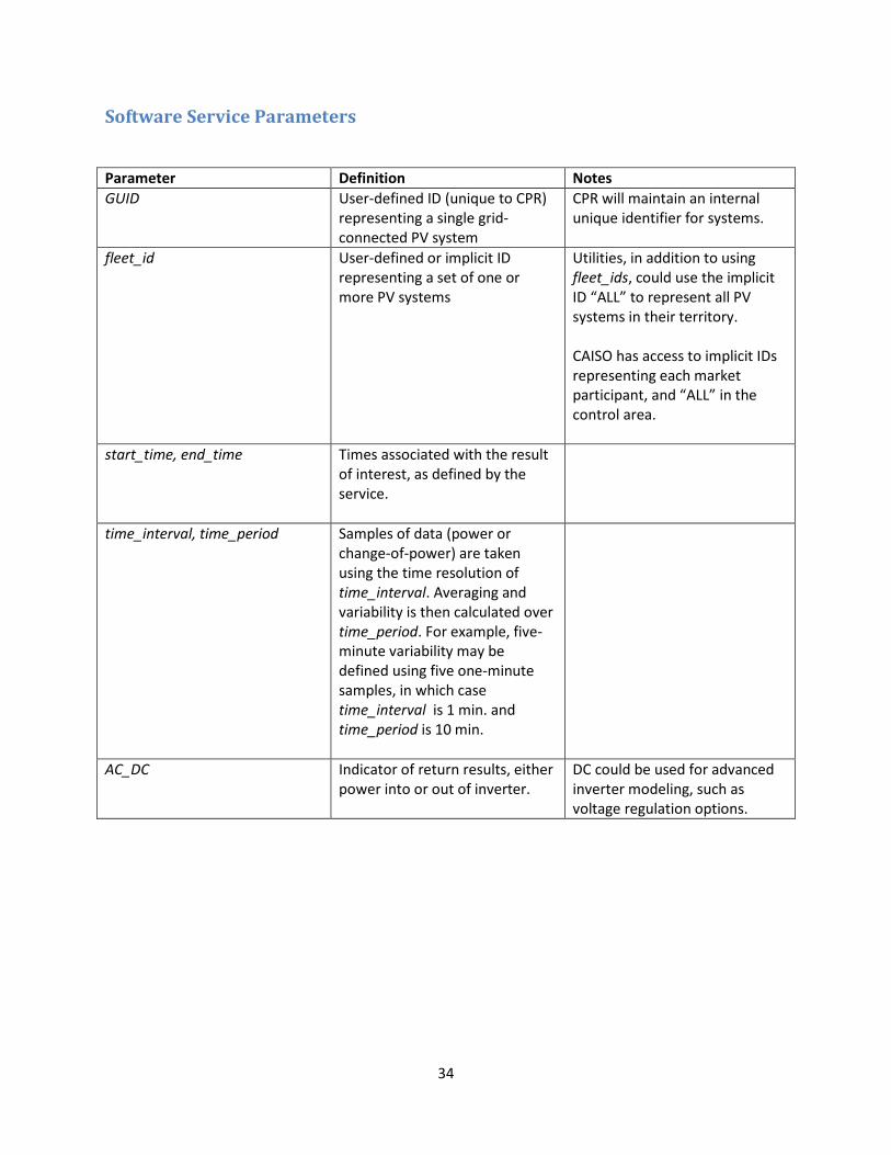
Software Service Parameters

Parameter Definition Notes GUID User-defined ID (unique to CPR)

representing a single grid-connected PV system

CPR will maintain an internal unique identifier for systems.

fleet_id User-defined or implicit ID representing a set of one or more PV systems

Utilities, in addition to using fleet_ids, could use the implicit ID “ALL” to represent all PV systems in their territory. CAISO has access to implicit IDs representing each market participant, and “ALL” in the control area.

start_time, end_time Times associated with the result of interest, as defined by the service.

time_interval, time_period Samples of data (power or change-of-power) are taken using the time resolution of time_interval. Averaging and variability is then calculated over time_period. For example, five-minute variability may be defined using five one-minute samples, in which case time_interval is 1 min. and time_period is 10 min.

AC_DC Indicator of return results, either power into or out of inverter.

DC could be used for advanced inverter modeling, such as voltage regulation options.

35

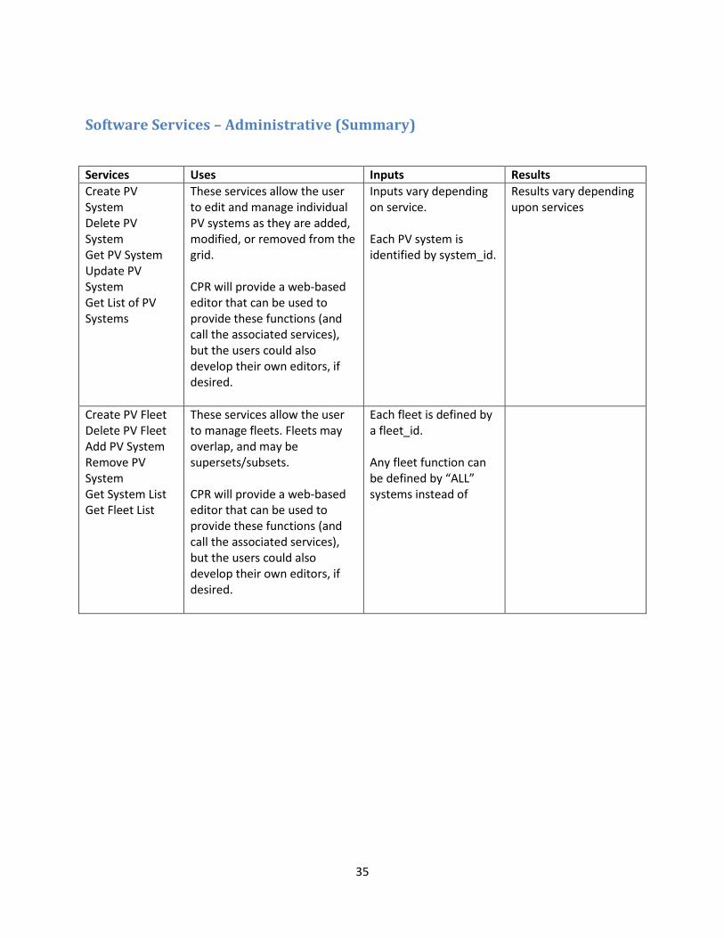
Software Services – Administrative (Summary)

Services Uses Inputs Results Create PV System Delete PV System Get PV System Update PV System Get List of PV Systems

These services allow the user to edit and manage individual PV systems as they are added, modified, or removed from the grid. CPR will provide a web-based editor that can be used to provide these functions (and call the associated services), but the users could also develop their own editors, if desired.

Inputs vary depending on service. Each PV system is identified by system_id.

Results vary depending upon services

Create PV Fleet Delete PV Fleet Add PV System Remove PV System Get System List Get Fleet List

These services allow the user to manage fleets. Fleets may overlap, and may be supersets/subsets. CPR will provide a web-based editor that can be used to provide these functions (and call the associated services), but the users could also develop their own editors, if desired.

Each fleet is defined by a fleet_id. Any fleet function can be defined by “ALL” systems instead of

36

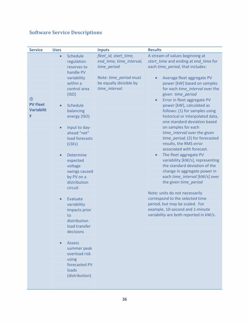
Software Service Descriptions

Service Uses Inputs Results PV Fleet Variability

• Schedule regulation reserves to handle PV variability within a control area (ISO)

• Schedule balancing energy (ISO)

• Input to day-ahead “net” load forecasts (LSEs)

• Determine

expected voltage swings caused by PV on a distribution circuit

• Evaluate

variability impacts prior to distribution load transfer decisions

• Assess

summer peak overload risk using forecasted PV loads (distribution)

fleet_id, start_time, end_time, time_interval, time_period Note: time_period must be equally divisible by time_interval.

A stream of values beginning at start_time and ending at end_time for each time_period, that includes:

• Average fleet aggregate PV power [kW] based on samples for each time_interval over the given time_period

• Error in fleet aggregate PV power [kW], calculated as follows: (1) for samples using historical or interpolated data, one standard deviation based on samples for each time_interval over the given time_period; (2) for forecasted results, the RMS error associated with forecast.

• The fleet aggregate PV variability [kW/s], representing the standard deviation of the change in aggregate power in each time_interval [kW/s] over the given time_period

Note: units do not necessarily correspond to the selected time period, but may be scaled. For example, 10-second and 1-minute variability are both reported in kW/s.

37

Example:

The California ISO schedules balancing energy and regulation reserves for the each hour of the day. It will dispatch resources hourly.

CAISO, 3/21/2011 00:00:00, 3/21/2011 23:59:59, 00:00:01, 01:00:00

… 00:14:00, 1246 kW, 130 kW, 96 kW/s 00:15:00, 1497 kW, 192 kW, 85 kW/s 00:16:00, 1635 kW, 226 kW, 75 kW/s …

PV Output

• Perform load flows using historical or forecast data.

GUID, start_time, end_time, time_interval, time_period, AC_DC Note: time_period must be equally divisible by time_interval.

Averaged output for every time_period with samples every time_interval between start_time and end_time. Values (AC or DC) are given for each PV system separately in the fleet. Results are preceded by the System Description.

Example: A distribution utility is considering transferring load from one substation to another, but wants to model the loading on a critical tie line before performing the operation.

ajZdvu398dfJK3elf, 3/21/2011 14:00:00, 3/21/2011 15:00:00, 00:01:00, 00:10:00, AC

<PV_1293> 14:00:00, 146 kW 14:10:00, 197 kW 14:20:00, 135 kW …

38

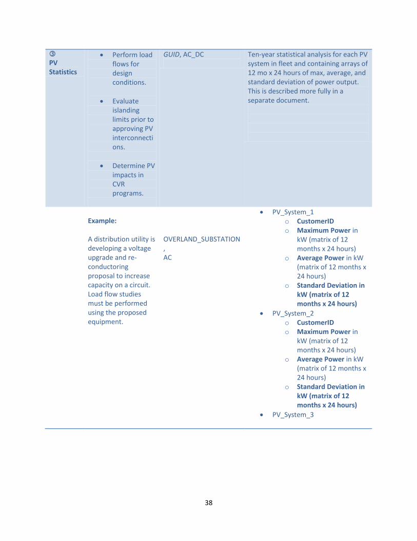
PV Statistics

• Perform load flows for design conditions.

• Evaluate

islanding limits prior to approving PV interconnections.

• Determine PV

impacts in CVR programs.

GUID, AC_DC

Ten-year statistical analysis for each PV system in fleet and containing arrays of 12 mo x 24 hours of max, average, and standard deviation of power output. This is described more fully in a separate document.

Example: A distribution utility is developing a voltage upgrade and re-conductoring proposal to increase capacity on a circuit. Load flow studies must be performed using the proposed equipment.

OVERLAND_SUBSTATION, AC

• PV_System_1 o CustomerID o Maximum Power in

kW (matrix of 12 months x 24 hours)

o Average Power in kW (matrix of 12 months x 24 hours)

o Standard Deviation in kW (matrix of 12 months x 24 hours)

• PV_System_2 o CustomerID o Maximum Power in

kW (matrix of 12 months x 24 hours)

o Average Power in kW (matrix of 12 months x 24 hours)

o Standard Deviation in kW (matrix of 12 months x 24 hours)

• PV_System_3

39

Appendix B: Optimal PV Location Identification Tool Description

Background There is an inherent tension between the value of power and the cost of power. The value of power is highest for on-site generation while the cost of power is lowest for off-site generation. This is because the value of power increases while the cost of power decreases with proximity to consumption. Power value increases near the point of consumption because delivery costs are reduced and other benefits are realized. Power cost decreases away from the point of consumption because generation is located far away from at least some loads due to the economies of scale associated with most types of generation.

PV, however, is one technology that helps to resolve this tension because it disobeys the economies of scale rule. PV is only mildly influenced by the size of the generating facility because the fundamental building block in a PV power generation system, the PV module, is the same whether it is used in a small PV system located at an individual’s house, or a very large PV plant located in the desert. This, along with other attributes associated with distributed PV generation, has captured people’s attention for more than two decades.

While there is substantial interest in distributed generation, utility planners currently lack the tools necessary to quickly and easily quantify the value of distributed PV based on when, where, what type, and how much PV is installed. The lack of tools is a result of several practical challenges in performing a distributed PV value analyses. One challenge is that an accurate evaluation requires time series PV output data specific to the location being evaluated. The PV modeling to produce the required data requires solar resource datasets, which, until recently, have been difficult to obtain. Another challenge is that the nature of the value components requires expertise from several different disciplines, including distribution planning, generation planning, regional renewable energy markets, and engineering economics.

As a result, utilities generally turn to third-party consultants to perform value analyses. Much of the work revolves around developing methodologies, encoding spreadsheet models, forming consensus within the different internal utility organizations, and writing reports.

Clean Power Research (CPR) has developed and applied analytical methodologies for calculating the value of distributed PV power generation for more than 20 years. It has performed such studies from as far back as analysis of the first installed distributed PV plant at PG&E’s Kerman substation in the early 1990s, to more recent studies (ref. [1] to [8]).

40

Introduction In New York, a recent NYS Public Service Ruling4 required that NYSERDA5 implement a geographic balancing program to site PV-electric generation projects in locations of highest utility value. In California, PV is reaching ever increasing levels of penetration in the distribution grid.

In response to these developments, both NYSERDA and the California Solar Initiative (CSI) program desire to explore ways to simplify the value assessment process. Rather than performing customized studies, one way to simplify the process is to take a “tools-based” approach. A “tools-based” approach is to develop a utility-oriented software valuation tool that would directly and immediately perform a valuation study on demand given a prescribed set of utility input data.

Utility planners could use such a tool to quickly and easily quantify value given the timing, location, type and quantity of PV capacity. This value indicator would include all of the key components treated in typical studies of this type: Energy Value, Generation Capacity Value, Environmental Value, Fuel Price Hedge Value, and T&D Capacity Value.

The “tools-based” approach offers several advantages over customized studies. The “tools-based” approach:

• Models PV generation for any location, hardware implementation, and orientation of interest. • Reduces costs by enabling users to perform studies in-house. • Embodies state-of-the-art valuation methodologies. • Provides consistency for all studies across the utility service territory. • Provides complete control over input assumptions. • Simplifies the performance of “what-if” studies by varying any of the assumptions. • Allows easy updating as circumstances change. • Makes the analysis easily repeatable. • Reduces computational errors through the use of stable, mature code libraries.

4 NYS Dept of Public Service, Order Authorizing Customer-Sited Tier Program Through 2015 And Resolving Geographic Balance And Other Issues Pertaining To The RPS Program, Issued 2 April 2010. 5 New York State Energy Research and Development Authority (www.nyserda.org)

41

Objective The overall objective of this project is to incorporate PV value analysis methodologies into a software service that equips users with the ability to perform such studies independently. The resulting software service will calculate the location-specific economic value of distributed PV generation from the perspective of the utility. The following value components will be included in the analysis:

• Energy Value • Generation Capacity Value • Environmental Value • Fuel Price Hedge Value • T&D Capacity Value • Loss Savings (incorporated in each of the value components)

The software service will be targeted for use by utility planners who support the geographic balancing program in NY and targeted PV installations in CA. Utility planners will use this information to determine the value of PV systems based on the specific location and configuration of those systems. The focus of this work is to determine the value of distributed PV to the utility. Subsequent work will expand the valuation to include value to society.

Overview The methodologies to be used in the present project will draw upon studies performed by CPR for other states and utilities. In these studies, the key value components provided by PV were determined by CPR, using utility-provided data and other economic data.

The ability to determine value on a site-specific basis is essential to these studies. For example, the T&D Capacity Value component depends upon the ability of PV to reduce peak loads on the circuits. An analysis of this value, then, requires:

• Hour-by-hour loads on distribution circuits of interest. • Hourly expected PV outputs corresponding to the location of these circuits and expected PV

system designs. • Local distribution expansion plan costs and load growth projections.

Units of Results This report presents the analysis in units of Present Value dollars ($). Each value component is calculated separately. Total value equals the sum of the individual value components.

The discounting convention assumed throughout the report is that energy-related values occur at the end of each year and that capacity-related values occur immediately (i.e., no discounting is required).6

The Present Value results can be can be converted to per unit value (Present Value $/kW) by dividing by the size of the PV system (kW). An example of this conversion is illustrated in Figure 14 for results from a 6 The effect of this will be most apparent in that the summations of cash flows start with the year equal to 1 rather than 0.

42

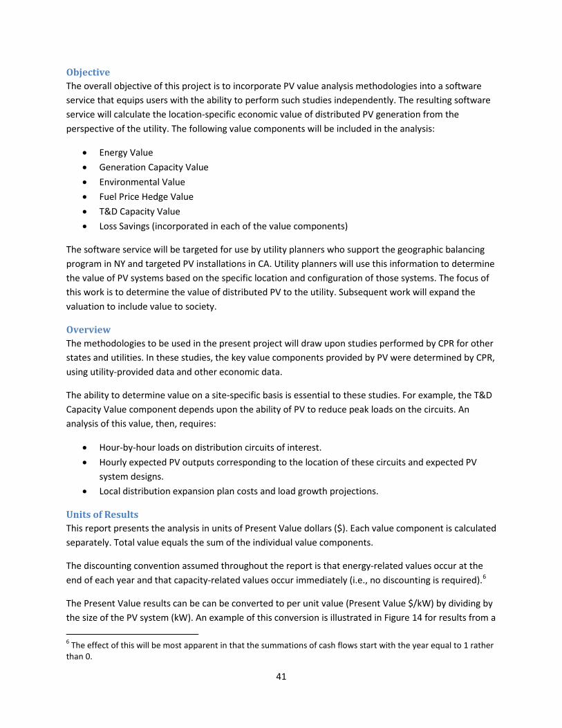
previous study. The y-axis presents the per unit value and the x-axis presents seven different PV system configurations. The figure illustrates how value components can be significantly affected by PV system configuration. For example, the tracking systems, by virtue of their enhanced energy production capability, provide greater generation benefits.

Figure 14. Sample results.

The Present Value results can also be converted to Levelized Value results ($/kWh). This is accomplished by dividing Present Value results by the total annual energy produced by the PV system and then multiplying by an economic factor.

43

PV Production And Loss Savings

PV System Output

Introduction An accurate PV value analysis begins with a detailed estimate of PV system output. Some of the energy-based value components may only require the total amount of energy produced per year. Other value components, however, such as the energy loss savings and the capacity-based value components, require hourly PV system output in order to determine the technical match between PV system output and the load. As a result, the PV value analysis requires time-, location-, and configuration-specific PV system output data.

For example, suppose that a utility wants to determine the value of a 1 MW fixed PV system oriented at a 30° tilt facing in the southwest direction located at distribution feeder “A”. Detailed PV output data that is time- and location-specific is required over some historical period, such as from Jan. 1, 2001 to Dec. 31, 2010.

Methodology It would be tempting to use a representative year data source such as NREL’s Typical Meteorological Year (TMY) data for purposes of performing a PV value analysis. While these data may be representative of long-term conditions, they are, by definition, not time-correlated with actual distribution line loading on an hourly basis and are therefore not usable in hourly side-by-side comparisons of PV and load. Peak substation loads measured, say, during a mid-August five-day heat wave must be analyzed alongside PV data that reflect the same five-day conditions. Consequently, a technical analysis based on anything other than time- and location-correlated solar data may give incorrect results.

CPR’s SolarAnywhere® and PVSimulator™ software services will be employed under this project to create time-correlated PV output data. SolarAnywhere is a solar resource database containing almost 14 years of time- and location-specific, hourly insolation data throughout the continental U.S. and Hawaii. PVSimulator, available in the SolarAnywhere Toolkit, is a PV system modeling service that uses this hourly resource data and user-defined physical system attributes in order to simulate configuration-specific PV system output.

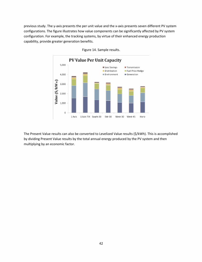
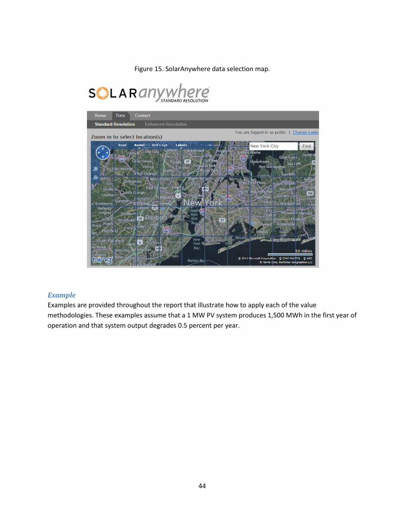
The SolarAnywhere data grid web interface is available at www.SolarAnywhere.com (or, see a sample in Figure 15 below). The structure of the data allows the user to perform a detailed technical assessment of the match between PV system output and load data (even down to a specific feeder). Together, these two tools enable the evaluation of the technical match between PV system output and loads for any PV system size and orientation.

Previous PV value analyses were generally limited to a small number of possible PV system configurations due to the difficulty in obtaining time- and location-specific solar resource data. This new value analysis software service, however, will integrate seamlessly with SolarAnywhere and PVSimulator. This will allow users to readily select any PV system configuration. This will allow for the evaluation of a comprehensive set of scenarios with essentially no additional study cost.

44

Figure 15. SolarAnywhere data selection map.

Example Examples are provided throughout the report that illustrate how to apply each of the value methodologies. These examples assume that a 1 MW PV system produces 1,500 MWh in the first year of operation and that system output degrades 0.5 percent per year.

45

Loss Savings

Introduction Distributed resources reduce system losses because they produce power in the same location that the power is consumed, bypassing the T&D system and avoiding the associated losses.

Loss savings are not treated as a stand-alone benefit under the convention used in this methodology. Rather, the effect of loss savings is included separately for each value component. For example, in the section that covers the calculation of Energy Value, the quantity of energy saved by the utility includes both the energy produced by PV and the amount that would have been lost due to heating in the wires if the load were served from a remote source. The total energy that would have been procured by the utility equals the PV energy plus avoided line losses. Loss savings can be considered a sort of “adder” for each benefit component.

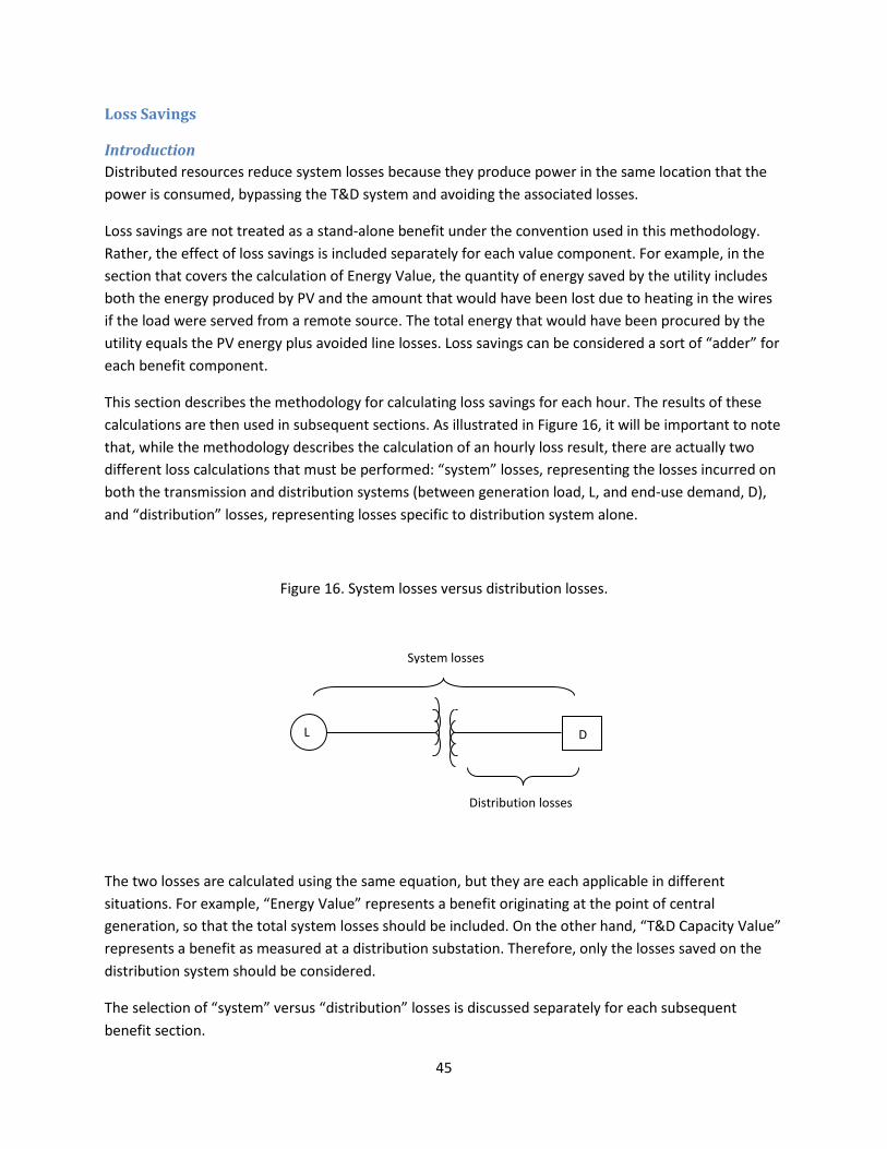
This section describes the methodology for calculating loss savings for each hour. The results of these calculations are then used in subsequent sections. As illustrated in Figure 16, it will be important to note that, while the methodology describes the calculation of an hourly loss result, there are actually two different loss calculations that must be performed: “system” losses, representing the losses incurred on both the transmission and distribution systems (between generation load, L, and end-use demand, D), and “distribution” losses, representing losses specific to distribution system alone.

Figure 16. System losses versus distribution losses.

The two losses are calculated using the same equation, but they are each applicable in different situations. For example, “Energy Value” represents a benefit originating at the point of central generation, so that the total system losses should be included. On the other hand, “T&D Capacity Value” represents a benefit as measured at a distribution substation. Therefore, only the losses saved on the distribution system should be considered.

The selection of “system” versus “distribution” losses is discussed separately for each subsequent benefit section.

L D

Distribution losses

System losses

46

Methodology One approach analysts have used to incorporate losses is to adjust energy- and capacity-related benefits based on the average system losses. This approach has been shown to be deficient because it fails to capture the true reduction in losses on a marginal basis. In particular, the approach underestimates the reduction in losses due to a peaking resource like PV. Results from earlier studies demonstrated that loss savings calculations may be off by more than a factor of two if not performed correctly [6].

For this reason, the present methodology will incorporate a calculation of loss savings on a marginal basis, taking into account the status of the utility grid when the losses occur. CPR has previously developed methodologies based on the assumption that the distributed PV resource is small relative to the load (e.g., [6], [9]). CPR has recently completed new research that expands this methodology so that loss savings can now be determined for any level of PV penetration.

Example Examples are provided throughout the report that illustrate how to apply each of the value methodologies. These examples assume that the PV system produces 1,500 MWh in the first year of operation and that generation system loss savings equal 150 MWh.

47

Value Component Methodology

Energy Value

Introduction Energy Value is the benefit that utility participants derive from using distributed PV generation to offset wholesale energy purchases or reduce generation costs. Each kWh generated by PV results in one less unit of energy that the utility needs to purchase or generate. In addition, distributed PV reduces system losses so that the cost of the wholesale generation that would have been lost must also be considered. The capacity value of generation is treated in a separate section.

Methodology Energy Value can be calculated by multiplying PV system output times the cost of the generation on the margin for each hour, summing for all hours over the year, and then discounting the results for each year over the life of the PV system.

There are two approaches to obtaining the marginal cost data. One approach is to obtain the marginal costs based on historical or projected market prices. The second approach is to obtain the marginal costs based on the cost of operating a representative generator that is on the margin.

Initially, it may be appealing to take the approach of using market prices. There are, however, several difficulties with this approach. One difficulty is that these tend to be hourly prices and thus require hourly PV system output data in order to calculate the economic value. This difficulty can be addressed by using historical prices and historical PV system output to evaluate what results would have been in the past and then escalating the results for future projections. A more serious difficulty is that, while hourly market prices could be projected for a few years into the future, the analysis needs to be performed over a much longer time period (typically 30 years). It is difficult to accurately project hourly market prices 30 years into the future.

A simpler approach is to explicitly specify the marginal generator and then to calculate the cost of the generation from this unit. It is typically assumed that the marginal generator offset by PV is a Combined Cycle Gas Turbine (CCGT) powered using natural gas. This approach includes the simplifying assumption that PV output always displaces energy from the same marginal unit. Given the uncertainties and complications in market price projections, the second, simpler approach is taken. Future versions of the software service may allow the user the option of choosing either approach.

The Energy Value equals the sum of the discounted fuel cost savings and the discounted O&M cost savings.

Example Table 1 illustrates how to calculate the Energy Value.

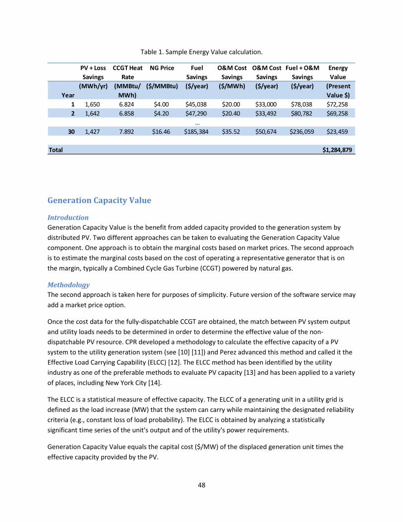
48

Table 1. Sample Energy Value calculation.

Generation Capacity Value

Introduction Generation Capacity Value is the benefit from added capacity provided to the generation system by distributed PV. Two different approaches can be taken to evaluating the Generation Capacity Value component. One approach is to obtain the marginal costs based on market prices. The second approach is to estimate the marginal costs based on the cost of operating a representative generator that is on the margin, typically a Combined Cycle Gas Turbine (CCGT) powered by natural gas.

Methodology The second approach is taken here for purposes of simplicity. Future version of the software service may add a market price option.

Once the cost data for the fully-dispatchable CCGT are obtained, the match between PV system output and utility loads needs to be determined in order to determine the effective value of the non-dispatchable PV resource. CPR developed a methodology to calculate the effective capacity of a PV system to the utility generation system (see [10] [11]) and Perez advanced this method and called it the Effective Load Carrying Capability (ELCC) [12]. The ELCC method has been identified by the utility industry as one of the preferable methods to evaluate PV capacity [13] and has been applied to a variety of places, including New York City [14].

The ELCC is a statistical measure of effective capacity. The ELCC of a generating unit in a utility grid is defined as the load increase (MW) that the system can carry while maintaining the designated reliability criteria (e.g., constant loss of load probability). The ELCC is obtained by analyzing a statistically significant time series of the unit's output and of the utility's power requirements.

Generation Capacity Value equals the capital cost ($/MW) of the displaced generation unit times the effective capacity provided by the PV.

PV + Loss Savings

CCGT Heat Rate

NG Price Fuel Savings

O&M Cost Savings

O&M Cost Savings

Fuel + O&M Savings

Energy Value

Year(MWh/yr) (MMBtu/

MWh)($/MMBtu) ($/year) ($/MWh) ($/year) ($/year) (Present

Value $)1 1,650 6.824 $4.00 $45,038 $20.00 $33,000 $78,038 $72,2582 1,642 6.858 $4.20 $47,290 $20.40 $33,492 $80,782 $69,258

…30 1,427 7.892 $16.46 $185,384 $35.52 $50,674 $236,059 $23,459

Total $1,284,879

49

Example Suppose that the ELCC equals 0.8 MW and the cost of capacity is $1,000,000 per MW. Generation Capacity value equals $1,000,000 x 0.8 =$800,000.

Environmental Value

Introduction It is well established that the environmental impact of PV is considerably smaller than that of fossil-based generation since PV is able to displace pollution associated with drilling/mining, and power plant emissions [15].

Methodology There are two general approaches to quantifying the Environmental Value of PV: a regulatory cost-based approach and an environmental/health cost-based approach.

The regulatory cost-based approach values the Environmental Value of PV based on the price of Renewable Energy Credits (RECs) or Solar Renewable Energy Credits (SRECs) that would otherwise have to be purchased to satisfy state Renewable Portfolio Standards (RPS). These costs are a preliminary legislative attempt to quantify external costs. They represent actual business costs faced by utilities in certain states.

An environmental/health cost-based approach quantifies the societal costs resulting from fossil generation. Each solar kWh displaces an otherwise dirty kWh and commensurately mitigates several of the following factors: greenhouse gases, SOx/NOx emissions, mining degradations, ground water contamination, toxic releases and wastes, etc., that are all present or postponed costs to society. Several exhaustive studies have estimated the environmental/health cost of energy generated by fossil-based generation [16], [17]. The results from environmental/health cost-based approach often vary widely and can be controversial.

The regulatory cost-based approach is taken for this software service because it represents the actual costs that would be incurred by the utility and because the data is more readily available. Note that loss savings are not typically included when evaluating the benefit using a regulatory cost-based approach.

Example Table 2 illustrates how to calculate the Environmental Value.

50

Table 2. Sample Environmental Value calculation.

Fuel Price Hedge Value

Introduction Solar-based generation is insensitive to the volatility of fuel prices while fossil-based generation is directly tied to fuel prices. Solar generation, therefore, offers a “hedge” against fuel price volatility. One way this has been accounted for is to quantify the value of PV’s hedge against fluctuating natural gas prices [6].

Methodology The key to calculating the Fuel Price Hedge Value is to effectively convert the fossil-based generation investment from one that has substantial fuel price uncertainty to one that has no fuel price uncertainty. This can be accomplished by entering into a binding commitment to purchase a lifetime’s worth of fuel to be delivered as needed. The utility could set aside the entire fuel cost obligation up front, investing it in risk-fee securities to be drawn from each year as required to meet the obligation. The approach uses two financial instruments: risk-free, zero-coupon bonds7 and a set of natural gas futures contracts.

Consider how this might work. Suppose that the CCGT operator wants to lock in a fixed price contract for a sufficient quantity of natural gas to operate the plant for one month, one year in the future. First, the operator would determine how much natural gas will be needed. If E units of electricity are to be generated and the heat rate of the plant is H, E * H BTUs of natural gas will be needed. Second, if the corresponding futures price of this natural gas is PNG Futures (in $ per BTU), then the operator will need E * H * PNG Futures dollars to purchase the natural gas one year from now. Third, the operator needs to set the money aside in a risk-free investment, typically a risk-free bond (rate-of-return of rrisk-free percent) to guarantee that the money will be available when it is needed one year from now. Therefore, the operator would immediately enter into a futures contract and purchase E * H * PNG Futures / (1+ rrisk-free)

7 A zero coupon bond does not make any periodic interest payments.

PV REC Price Environmental Value

Environmental Value

Year (MWh/yr) ($/MWh) ($/year) (Present Value $)1 1,500 $25.00 $37,500 $34,7222 1,493 $25.75 $38,432 $32,949

…30 1,297 $58.91 $76,415 $7,594

Total $538,846

51

dollars’ worth of risk-free, zero-coupon bonds in order to guarantee with certainty that the financial commitment (to purchase the fuel at the contract price at the specified time) will be satisfied.8

This calculation is repeated over the life of the plant to calculate the Fuel Price Hedge value.

Example Table 3 illustrates how to calculate the Fuel Price Hedge Value.

Table 3. Sample Fuel Price Hedge Value calculation.9

T&D Capacity Value

Introduction The benefit that can be most affected by the PV system’s location is the T&D Capacity Value. The T&D Capacity Value depends on the existence of location-specific projected expansion plan costs to ensure reliability over the coming years as the loads grow. Capacity-constrained areas where loads are expected to reach critical limits present more favorable locations for PV to the extent that PV will relieve the constraints, providing more value to the utility than those areas where capacity is not constrained.

Distributed PV generation reduces the burden on the distribution system. It appears as a “negative load” during daylight hours from the perspective of the distribution operator. Distributed PV may be considered equivalent to distribution capacity from the perspective of the distribution planner, provided that PV generation occurs at the time of the local distribution peak.

Distributed PV capacity located in an area of growing loads allows a utility planner to defer capital investments in distribution equipment such as substations and lines. The value is determined by the avoided cost of money due to the capital deferral.

8 [E * H * PNG Futures / (1+ rrisk-free)] * (1+ rrisk-free) = E * H * PNG Futures 9 The Economic Factor represents the effect of discounting using a “risky” discount rate versus discounting the certain fuel cost at the risk-free rate.

PV + Loss Savings

CCGT Heat Rate NG Futures Price

Fuel Savings

Economic Factor

Hedge Value

Year (MWh) (MMBtu/MWh) ($/MMBtu) ($/year) (Present Value $)1 1,650 6.824 $4.00 $45,038 0.04 $1,6042 1,642 6.858 $4.20 $47,290 0.07 $3,179

…30 1,427 7.892 $16.46 $185,384 0.21 $38,734

Total $641,211

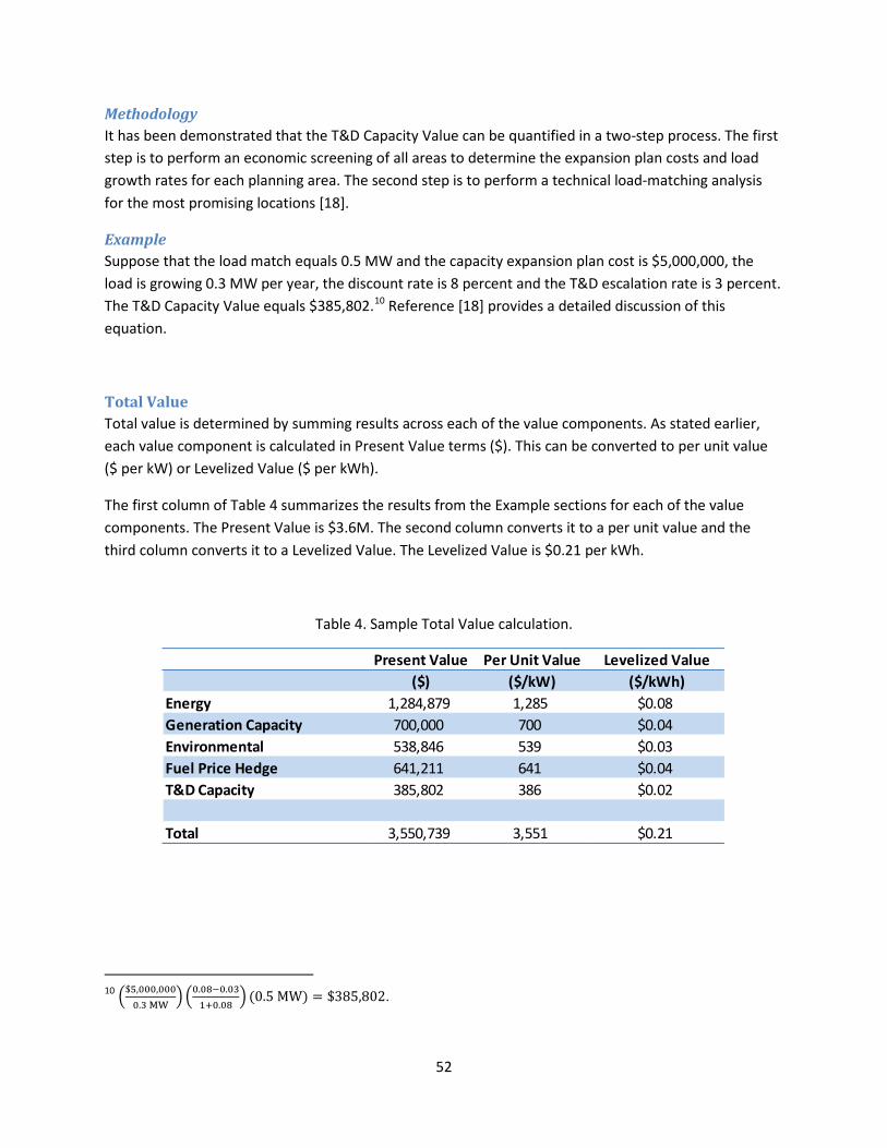
52

Methodology It has been demonstrated that the T&D Capacity Value can be quantified in a two-step process. The first step is to perform an economic screening of all areas to determine the expansion plan costs and load growth rates for each planning area. The second step is to perform a technical load-matching analysis for the most promising locations [18].

Example Suppose that the load match equals 0.5 MW and the capacity expansion plan cost is $5,000,000, the load is growing 0.3 MW per year, the discount rate is 8 percent and the T&D escalation rate is 3 percent. The T&D Capacity Value equals $385,802.10 Reference [18] provides a detailed discussion of this equation.

Total Value Total value is determined by summing results across each of the value components. As stated earlier, each value component is calculated in Present Value terms ($). This can be converted to per unit value ($ per kW) or Levelized Value ($ per kWh).

The first column of Table 4 summarizes the results from the Example sections for each of the value components. The Present Value is $3.6M. The second column converts it to a per unit value and the third column converts it to a Levelized Value. The Levelized Value is $0.21 per kWh.

Table 4. Sample Total Value calculation.

10 �$5,000,000

0.3 MW� �0.08−0.03

1+0.08� (0.5 MW) = $385,802.

Present Value Per Unit Value Levelized Value($) ($/kW) ($/kWh)

Energy 1,284,879 1,285 $0.08Generation Capacity 700,000 700 $0.04Environmental 538,846 539 $0.03Fuel Price Hedge 641,211 641 $0.04T&D Capacity 385,802 386 $0.02

Total 3,550,739 3,551 $0.21

53

References [1]. Hoff, T. E., Wenger, H. J., and Farmer, B. K. “Distributed Generation: An Alternative to Electric Utility Investments in System Capacity,” Energy Policy 24(2):137-147, 1996.

[2]. Hoff, T. E. Final Results Report with a Determination of Stacked Benefits of Both Utility-Owned and Customer-Owned PV Systems: Deliverable 1.3.5.2, SMUD Report, 2002.

[3]. Hoff, T. E., and Margolis, R. Distributed Photovoltaics in New Jersey, NREL Report, 2003. www.cleanpower.com/research/distributedgeneration/DistributedPVInNewJersey.pdf.

[4]. Hoff, T. E., Norris, B. L., and Wayne, G. Potential Economic Benefits of Distributed Photovoltaics to the Nevada Power Company. Report, 2003. www.cleanpower.com/Content/Documents/research/distributedgeneration/NevadaPower2003.pdf

[5]. Hoff, T. E. and Margolis, R. M. Moving Towards a More Comprehensive Framework to Evaluate Distributed Photovoltaics. Report, 2005. www.cleanpower.com/Content/Documents/research/customerPV/EvaluationFramework.pdf

[6]. Hoff, T.E., Perez, R., Braun, G., Kuhn, M., and Norris, B. The Value of Distributed Photovoltaics to Austin Energy and the City of Austin, 2006. www.cleanpower.com/Content/Documents/research/distributedgeneration/AE_PV_ValueReport.pdf.

[7]. Norris, B. L., Hoff, T. E., Perez, R. PV Value Analysis for We Energies, 2009

[8]. Perez, R. Zweibel, K., and Hoff, T. E. “Solar Power Generation in the US: Too expensive, or a bargain?” Submitted to Energy Policy. 2011.

[9]. Hoff, T. and Shugar, D. S., “The Value of Grid-Support Photovoltaics In Reducing Distribution System Losses,” IEEE Transactions on Energy Conversion, 10(9): 569-576.,1995.

[10]. Garver, L. L. “Effective Load Carrying Capability of Generating Units. IEEE Transactions, Power Apparatus and Systems.” Vol. Pas-85, no. 8, 1966.

[11]. Hoff, T. “Calculating Photovoltaics' Value: A Utility Perspective,” IEEE Transactions on Energy Conversion 3: 491-495, 1988.

[12]. Perez, R., Seals, R., and Stewart, R. “Assessing the Load Matching Capability of Photovoltaics for US Utilities Based Upon Satellite-Derived Insolation Data,” IEEE Transactions, pp. 1146-1149 (23d. PV Specialists, Louisville, KY), 1993.

[13]. Hoff, T., Perez, R. Ross, JP, and Taylor, M. Photovoltaic Capacity Valuation Methods, Solar Electric Power Association Report #02-08, 2008.

[14]. Hoff, T. E. and Perez, R. Shining on the Big Apple: Satisfying New York City’s Peak Electrical Needs with PV. Report, 2008. www.cleanpower.com/Content/Documents/research/distributedgeneration/PVForNewYorkCity.pdf.

54

[15]. Fthenakis, V., Kim, H.C., Alsema, E., “Emissions from Photovoltaic Life Cycles”. Environmental Science and Technology, 42(6): p. 2168-2174, 2008.

[16]. Devezeaux J. G. “Environmental Impacts of Electricity Generation”. 25th Uranium Institute Annual Symposium. London, UK, 2000.

[17]. Epstein, P. “Full cost accounting for the life cycle of coal”. Annals of the New York Academy of Sciences, 2011.

[18]. Hoff, T. E. “Identifying Distributed Generation and Demand Side Management Investment Opportunities,” The Energy Journal: 17(4), 1996.