final report, er-2338
TRANSCRIPT
Final Report, ER-2338 June 25, 2020
FINAL REPORT
Environmental Restoration Project
CO2 Radiocarbon Analysis to Quantify Organic Contaminant Degradation, MNA, and Engineered
Remediation Approaches
Project Number: ER-2338
Lead: US Naval Research Laboratory Washington, DC
Thomas J. Boyd, Michael T. Montgomery; Chemical Dynamics and Diagnostics Branch Chemistry Division, US NRL, Washington, DC Richard H. Cuenca, Yutaka Hagimoto; Hydrologic Engineering, Inc. Corvallis, OR Maria Vernet, Jennifer Gonzalez; IOD, Scripps Institution of Oceanography, La Jolla, CA
June 2020
REPORT DOCUMENTATION PAGE
Standard Form 298 (Rev. 8/98) Prescribed by ANSI Std. Z39.18
Form Approved OMB No. 0704-0188
The public reporting burden for this collection of information is estimated to average 1 hour per response, including the time for reviewing instructions, searching existing data sources, gathering and maintaining the data needed, and completing and reviewing the collection of information. Send comments regarding this burden estimate or any other aspect of this collection of information, including suggestions for reducing the burden, to Department of Defense, Washington Headquarters Services, Directorate for Information Operations and Reports (0704-0188), 1215 Jefferson Davis Highway, Suite 1204, Arlington, VA 22202-4302. Respondents should be aware that notwithstanding any other provision of law, no person shall be subject to any penalty for failing to comply with a collection of information if it does not display a currently valid OMB control number. PLEASE DO NOT RETURN YOUR FORM TO THE ABOVE ADDRESS.
2. REPORT TYPE
5b. GRANT NUMBER
5c. PROGRAM ELEMENT NUMBER
5e. TASK NUMBER
5f. WORK UNIT NUMBER
8. PERFORMING ORGANIZATION
11. SPONSOR/MONITOR'S REPORTNUMBER(S)
13. SUPPLEMENTARY NOTES
16. SECURITY CLASSIFICATION OF:a. REPORT b. ABSTRACT c. THIS PAGE
17. LIMITATION OFABSTRACT
18. NUMBEROFPAGES
9. SPONSORING/MONITORING AGENCY NAME(S) AND ADDRESS(ES) 10. SPONSOR/MONITOR'S ACRONYM(S)
12. DISTRIBUTION/AVAILABILITY STATEMENT
19b. TELEPHONE NUMBER (Include area code)
5d. PROJECT NUMBER ER-2338
REPORT NUMBER
ER-2338
ER-2338
SERDP
UNCLASSUNCLASS UNCLASS UNCLASS
19a. NAME OF RESPONSIBLE PERSON Thomas Boyd
6. AUTHOR(S)Thomas J. Boyd, Michael T. MontgomeryChemical Dynamics and Diagnostics Branch Chemistry Division, US NRL
Richard H. Cuenca, Yutaka HagimotoHydrologic Engineering, Inc.
Maria Vernet, Jennifer GonzalezScripps Institution of Oceanography
5a. CONTRACT NUMBER
3. DATES COVERED (From - To)
202-404-6424
7. PERFORMING ORGANIZATION NAME(S) AND ADDRESS(ES) Naval Research Laboratory 4555 Overlook Ave., SWWashington, DC 20375
DISTRIBUTION STATEMENT A. Approved for public release: distribution unlimited.
1. REPORT DATE (DD-MM-YYYY) 30/06/2020 SERDP Final Report
4. TITLE AND SUBTITLE
CO2 Radiocarbon Analysis to Quantify Organic Contaminant Degradation, MNA, and Engineered Remediation Approaches
74
Strategic Environmental Research and Development Program (SERDP)4800 Mark Center Drive, Suite 16F16Alexandria, VA 22350-3605
14. ABSTRACTThe Department of Defense (DoD) faces billion-dollar expenditures for environmental cleanup in the United States. Prohibitive cleanup costs make treatment strategies such as monitored natural attenuation (MNA), enhanced passive remediation (EPR) or low-cost engineered solutions attractive remediation alternatives for reaching Response Complete (RC) status. Several lines of converging evidence are seen as necessary to establish reasonable evidence for in situ bioremediation or natural attenuation. It is generally accepted that no single analysis or combination of ex situ or laboratory tests provides an accurate confirmation or rate for biodegradation under in situ conditions (1). Similarly, reports sponsored by DoD, the DOE and the Environmental Protection Agency (EPA) advocate collection of a wide array of data in order to attempt confirmation of contaminant attenuation and predict timescale(s) for remediation (2, 3).
15. SUBJECT TERMSCO2 Radiocarbon Analysis, Quantify Organic Contaminant Degradation, MNA, Engineered Remediation Approaches
Final Report, ER-2338 June 25, 2020
i
Table of Contents
Table of Contents ........................................................................................................................................... i List of Figures ................................................................................................................................................ ii List of Tables ................................................................................................................................................ iii List of Acronyms and Abbreviations and Keywords ...................................................................................... v Acknowledgements ...................................................................................................................................... vi Abstract ....................................................................................................................................................... vii
Introduction ............................................................................................................................................ vii Objectives ................................................................................................................................................ vii Technical Approach ................................................................................................................................ viii Results and Discussion ............................................................................................................................. ix Implications for Future Research and Benefits ........................................................................................ xi
Objective ....................................................................................................................................................... 1 Background ................................................................................................................................................... 2
Site Descriptions ....................................................................................................................................... 5 IR-5 Unit 2, NASNI ................................................................................................................................. 5 OU-19/20, NASNI .................................................................................................................................. 7 IR-17, Indian Head NSWC ...................................................................................................................... 9 IR-57, Indian Head NSWC. ..................................................................................................................... 9
Materials and Methods ........................................................................................................................... 10 IR-5 U2 Hardware and Field Sampling. ............................................................................................... 10 OU19/20, IR-17/IR-57 Hardware and Field Sampling. ........................................................................ 11 Water Quality Analyses ....................................................................................................................... 12 Soil Gas Methane Concentrations ...................................................................................................... 12 Radiocarbon Analysis .......................................................................................................................... 13 CO2 Production Rate Analysis ............................................................................................................. 13 Zone of Influence Model/Simulation .................................................................................................. 13 Determining the Contaminant Respired ............................................................................................. 14
Results and Discussion ................................................................................................................................ 15 IR-5 Unit 2 ............................................................................................................................................... 15
ZOI Simulations ................................................................................................................................... 15 Water Quality Measurements ............................................................................................................ 17 Respiration .......................................................................................................................................... 18 Radiocarbon Analysis .......................................................................................................................... 18 Conversion from Radiocarbon and Respiration to cVOC Degradation ............................................... 19 Site-Wide TCE Degradation and Long-Term Remediation .................................................................. 32
OU-19/20 NASNI ..................................................................................................................................... 34 ZOI Simulations ................................................................................................................................... 34 Water Quality Measurements ............................................................................................................ 34 Respiration .......................................................................................................................................... 35 Radiocarbon Analysis .......................................................................................................................... 35 Conversion from Radiocarbon and Respiration to cVOC Degradation ............................................... 35
Final Report, ER-2338 June 25, 2020
ii
Site-Wide TCE Degradation and Long-Term Remediation .................................................................. 45 IR-17 Indian Head .................................................................................................................................... 47
ZOI Simulations ................................................................................................................................... 47 Water Quality Measurements ............................................................................................................ 48 Respiration .......................................................................................................................................... 48
IR-57 Indian Head .................................................................................................................................... 48 ZOI Simulations ................................................................................................................................... 49 Water Quality Measurements ............................................................................................................ 49 Respiration .......................................................................................................................................... 50
Radiocarbon – IR-17 and IR-57................................................................................................................ 50 Conclusions and Implications for Future Research / Implementation ....................................................... 53 Literature Cited ........................................................................................................................................... 56 Appendix A. Supporting Data ...................................................................................................................... 59 Appendix B. List of Scientific / Technical Publications ................................................................................ 60
List of Figures Figure 1. CO2 radiocarbon age upgradient, above, and downgradient of petroleum-based chemical plume. ........................................................................................................................................................... 2 Figure 2. 14C Analysis in a "Natural Lab" ....................................................................................................... 3 Figure 3. IR Site 5 (all units)........................................................................................................................... 5 Figure 4. IR Site 5 Unit 2 (Shaw 2013) ........................................................................................................... 6 Figure 5. OU-19/20 NASNI (Noreas, 2014) ................................................................................................... 7 Figure 6. IR-17 NSWC Indian Head (CH2MHill) ............................................................................................. 8 Figure 7. IR-57 NSWC Indian Head showing upper and mid-plumes (Osage) .............................................. 9 Figure 8. Well Headspace Gas Recirculating Pumps, Sealed ...................................................................... 10 Figure 9. Solar Power Distribution System in Place .................................................................................... 11 Figure 10. Well Headspace CO2 Collection System ..................................................................................... 11 Figure 11. NaOH Trap Showing Support and Reservoir .............................................................................. 12 Figure 12. Well Cap Sealed in Place with Sparge Line and Check Valve ..................................................... 12 Figure 13. Calibrated CO2 Distribution. ....................................................................................................... 16 Figure 14. Historical cVOC Contamination IR-5 U2 ..................................................................................... 19 Figure 15. TCE Degradation 11/06/14-11/24/14 ........................................................................................ 21 Figure 16. TCE Degradation 11/24/14-12/05/14 ........................................................................................ 21 Figure 17. TCE Degradation 12/05/14-12/18/14 ........................................................................................ 22 Figure 18. TCE Degradation 12/19/14-01/05/15 ........................................................................................ 22 Figure 19. TCE Degradation 01/18/15-01/27/15 ........................................................................................ 23 Figure 20. TCE Degradation 02/02/15-02/16/15 ........................................................................................ 23 Figure 21. TCE Degradation 02/16/15-03/09/15 ........................................................................................ 24 Figure 22. TCE Degradation 03/10/15-04/10/15 ........................................................................................ 24 Figure 23. TCE Degradation 04/10/15-04/30/15 ........................................................................................ 25 Figure 24. TCE Degradation 04/30/15-05/20/15 ........................................................................................ 25 Figure 25. TCE Degradation 05/20/15-06/01/15 ........................................................................................ 26
Final Report, ER-2338 June 25, 2020
iii
Figure 26. TCE Degradation 06/01/15-06/15/15 ........................................................................................ 26 Figure 27. TCE Degradation 06/15/15-06/28/15 ........................................................................................ 27 Figure 28. TCE Degradation 06/28/15-07/20/15 ........................................................................................ 27 Figure 29. TCE Degradation 07/20/15-08/18/15 ........................................................................................ 28 Figure 30. TCE Degradation 08/18/15-08/27/15 ........................................................................................ 28 Figure 31. TCE Degradation 08/27/15-09/13/15 ........................................................................................ 29 Figure 32. TCE Degradation 09/13/15-10/06/15 ........................................................................................ 29 Figure 33. TCE Degradation 10/06/15-11/03/15 ........................................................................................ 30 Figure 34. TCE Degradation 11/03/15-11/30/15 ........................................................................................ 30 Figure 35. TCE Degradation 11/30/15-12/17/15 ........................................................................................ 31 Figure 36. Total Site-Wide TCE Degradation and Rainfall Over the Entire Sampling Period ...................... 33 Figure 37. OU-19/20 at NASNI, San Diego, CA ............................................................................................ 35 Figure 38. OU-19 TCE Degradation 12/17/15-02/02/16 ............................................................................. 36 Figure 39. OU-19 TCE Degradation 02/02/16-03/19/16 ............................................................................. 37 Figure 40. OU-19 TCE Degradation 03/19/16-05/19/16 ............................................................................. 37 Figure 41. OU-19 TCE Degradation 05/19/16-07/18/16 ............................................................................. 38 Figure 42. OU-19 TCE Degradation 07/18/16-08/29/16 ............................................................................. 38 Figure 43. OU-19 TCE Degradation 08/29/16-10/13/16 ............................................................................. 39 Figure 44. OU-19 TCE Degradation 10/13/16-02/23/17 ............................................................................. 39 Figure 45. OU-20 TCE Degradation 07/21/15-08/29/15 ............................................................................. 40 Figure 46. OU-20 TCE Degradation 08/29/15-11/02/15 ............................................................................. 40 Figure 47. OU-20 TCE Degradation 11/02/15-12/17/15 ............................................................................. 41 Figure 48. OU-20 TCE Degradation 12/17/15-02/02/16 ............................................................................. 41 Figure 49. OU-20 TCE Degradation 02/02/16-03/18/16 ............................................................................. 42 Figure 50. OU-20 TCE Degradation 03/19/16-05/19/16 ............................................................................. 42 Figure 51. OU-20 TCE Degradation 05/19/16-07/18/16 ............................................................................. 43 Figure 52. OU-20 TCE Degradation 07/18/16-08/29/16 ............................................................................. 43 Figure 53. OU-20 TCE Degradation 08/29/16-10/13/16 ............................................................................. 44 Figure 54. OU-20 TCE Degradation 10/13/16-02/23/17 ............................................................................. 44 Figure 55. cVOC Degradation and Rainfall at OU-19/20 ............................................................................. 46 Figure 56. CaCO3 and Organic Acid Concentrations, IR-17 ......................................................................... 48 Figure 57. CaCO3 Relation to pH, Alkalinity and Organic Acids, IR-57 ........................................................ 50 Figure 58. New Distillation Line (early 2019) .............................................................................................. 51 Figure 59. TCE degradation 11/03/15-11/30/15 ........................................................................................ 53
List of Tables Table 1. Hydrogeologic Parameters Used in IR-5 U2 ZOI Model(s) ............................................................ 15 Table 2. Selected Cation Concentrations and pH for IR-5 U2 ..................................................................... 18 Table 3. TCE Degradation Over IR-5 U2 by Time Bin .................................................................................. 32 Table 4. Hydrogeologic Parameters Used for OU-19/20 ZOI models ......................................................... 34 Table 5. Selected Cation and pH Measurements for OU-19/20 ................................................................. 34 Table 6. TCE degradation Over OU-19 by Time Bin .................................................................................... 45

Final Report, ER-2338 June 25, 2020
iv
Table 7. TCE Degradation Over OU-20 by Time Bin .................................................................................... 45 Table 8. IR-17 Analyses by Sample Time Bins ............................................................................................. 47 Table 9. Hydrogeologic Parameters Used for IR-17 ZOI Models ................................................................ 47 Table 10. IR-57 Analyses by Sample Time Bins ........................................................................................... 49 Table 11. Mean Hydrogeologic Parameters Used for IR-57 ZOI Models .................................................... 49
Final Report, ER-2338 June 25, 2020
v
List of Acronyms and Abbreviations and Keywords bgs below ground surface CH chlorinated hydrocarbons COI contaminants of interest COC contaminants of concern cVOC chlorinated volatile organic compound δ13C Delta C-13 (stable isotope ratio) ∆14C Delta C-14 (radiocarbon isotope ratio) DIC dissolved inorganic carbon (dissolved CO2) DNAPL dense non-aqueous phase liquid DO dissolved oxygen DoD U.S. Department of Defense EPA U.S. Environmental Protection Agency EVO emulsified vegetable oil IR Installation Restoration LNAPL light non-aqueous phase liquid LTM long-term monitoring MNA monitored natural attenuation NAVBASE Naval Base NAVFAC LANT Naval Facilities Engineering Command Atlantic NAVFAC Northwest Naval Facilities Engineering Command Northwest NAVFAC Southwest Naval Facilities Engineering Command Southwest Navy U.S. Navy NRL Naval Research Laboratory OU Operable Unit QA quality assurance QC quality control ROD Record of Decision RPM Remedial Project Manager SAP Sampling and Analysis Plan SOP standard operating procedure TCA trichloroethane TCE trichloroethylene VOC volatile organic compound ZOI Zone of Influence Keywords: biodegradation, petroleum-source, fossil end-member, radiocarbon, radiocarbon-depleted, monitoring well, headspace.
Final Report, ER-2338 June 25, 2020
vi
Acknowledgements This project was made possible by funding through SERDP and co-funding by RPMs at NAVFAC Southwest, Northwest and LANT. Site logistics were aided by RPMs (access, historical documents, storage space, shipping/receiving, and site discussions). The project team would like to thank Michael Pound, Alex Scott, Phil Nenninger and Malcolm Gander for additional site access and seed funding. The project was also supported by on-base contractors who provided critical information on site conditions and helped steer efforts toward the most fruitful outcomes. We wish to thank Todd Wiedemeier (which sadly can no longer be done personally), Vitthal Hosangadi (Noreas), Glen Wyatt (Tetratech), Brian White (Shaw), Erika Thompson (Shaw), Andrew Louder (NAVFAC) and Gunarti Coghlan (NAVFAC) for site-specific information and logistic support. We also wish to thank co-participants in a limited field study which led to ESTCP transition comparing and cross-validating methods; Julio Zimbron (E-Flux, LLC), Chuck Newell (GSI), and John T. Wilson (Scissortail Environmental).
Final Report, ER-2338 June 25, 2020
vii
Abstract Introduction The Department of Defense (DoD) faces billion-dollar expenditures for environmental cleanup in the United States. Prohibitive cleanup costs make treatment strategies such as monitored natural attenuation (MNA), enhanced passive remediation (EPR) or low-cost engineered solutions attractive remediation alternatives for reaching Response Complete (RC) status. Several lines of converging evidence are seen as necessary to establish reasonable evidence for in situ bioremediation or natural attenuation. It is generally accepted that no single analysis or combination of ex situ or laboratory tests provides an accurate confirmation or rate for biodegradation under in situ conditions (1). Similarly, reports sponsored by DoD, the DOE and the Environmental Protection Agency (EPA) advocate collection of a wide array of data in order to attempt confirmation of contaminant attenuation and predict timescale(s) for remediation (2, 3). SERDP/ESTCP priorities include: • Quantifying natural attenuation capacities; • Reducing uncertainty; • Assessing and managing spatial variability; • Determining side-effects of remediation; • Optimizing existing technologies; • Understanding emerging contaminants; • Improving long-term monitoring; • Source delineation and characterization and source zone characterization and flux analysis; • Bioaugmentation and source zone bioremediation; and • Effects of treatment amendments (SERDP/ESTCP 2002; Leeson and Stroo 2011). The ultimate end-product for organic contaminant degradation is CO2– representing a complete conversion to a relatively harmless product. A methodological limitation for current technologies is the inability to conclusively link contaminants, daughter products, electron acceptors, hydrogeological parameters, and in some cases, biological activities to actual contaminant removal (e.g., conversion to CO2). This study combines CO2 radiocarbon measurements with CO2 flux measurements to quantify contaminant carbon conversion to CO2– and thus complete degradation.
Objectives This project's objective is to combine CO2 respiration, CO2 radiocarbon content and a Zone of Influence (ZOI) model to calculate chlorinated hydrocarbon degradation occurring at real DoD contaminated sites. Radiocarbon analysis will measure the fraction of petroleum-source in the CO2 pool. To determine COI degradation rate, we will measure the CO2 production rate by circulating groundwater well headspace through a CO2 trap over time or use a passive trap suspended in the wells’ headspace. A well zone of influence (ZOI) can be calculated using process-based simulation models of gas transport in porous media (4). The ZOI model and CO2 production rate will be used to determine the overall CO2 production rate per soil unit. Given the fraction of
Final Report, ER-2338 June 25, 2020
viii
CO2 derived from a petroleum-source and CO2 produced per soil unit (cubic meter for example), the contaminant degradation rate can be determined over both time and space. This will support all research needs outlined in the SERDP needs section (5, 6) – enhancing management, assessing efficacy or fully quantifying natural attenuation capacities. This technology is straightforward and commercially-available, and will provide two key answers for site management and remediation efficacy (both active and passive) that have not been available:
• Is remediation occurring? We will be able to track the amount (percentage basis) of the degradation end product (CO2). On the basis of this one measurement, a site manager will be able to definitively state whether (bio)degradation is occurring or not.
• At what rate is the remediation occurring? By measuring the proportion of fossil fuel-derived CO2 and the CO2 production rate over time, we will be able to calculate the rate of (bio)degradation occurring on-site. Using groundwater transport models and given an estimated size or volume of source material and plume dimensions, a much more accurate estimation of the time for remediation can be predicted:
( ) remediate to time tcontaminan source tcontaminan fromCO
) (i.e. unit time 2
≅
g
gdays
Technical Approach The technical approach for the project is relatively well defined. It involves measuring the CO2 production over unit time (respiration) and determining a radiocarbon age for that respired product. If the CO2 is radiocarbon-depleted relative to a background site where natural organic matter is the only respiratory substrate, the radiocarbon-depleted CO2 must be derived from the petroleum-sourced contaminant. By coupling the respiration rate and the differential respiration product derived from the contaminant, a contaminant degradation rate can be determined. Developing a model based on site hydrogeologic parameters which determines the volume sampled during each respiration measurement allows scaling contaminant degradation rate spatially and interpolation between wells sampled as above allows site-wide contaminant degradation estimates. Respiration was measured using CO2 traps deployed either adjacent to or within the casing of groundwater monitoring wells. The external traps were supplied with gas lines so that in-well headspace gas could be continously cycled over the trap material. Due to the nature of many sites (operable units), actively cycled traps and the associated power support equipment were not practical. Passive traps were developed that were not as efficient (slower timeframe to equilibrium) but effective at trapping CO2 evolved from groundwater and liberated into well headspaces over deployment time. In all cases, trap material was recovered after 2-10 weeks, dissolved in a known amount of CO2-free water, and analyzed for CO2 content. Collection rate was determined as the amount of CO2 collected per unit time (hours or days). Respiration was
Final Report, ER-2338 June 25, 2020
ix
calculated as the collection rate minus the lowest collection rate value determined for the entire field site deployment with the assumption that the lowest value could represent equilibrium trapping alone (meaning no respiration, but the in-ground residual CO2 pool would be trapped due to equilibrium forces). The final component was to develop ZOI models for each well and time-point using hydrogeologic parameters measured on-site (c.f. Tables, 4, 9 and 11) and CO2 collection rates. ZOI models were developed using MODFLOW-2005 and front-ends tailored to contaminant and CO2 diffusion (MT3DMS). Parameterized simulations for each well and time-point had volumetric outputs (e.g. m3) which represented the volume sampled to obtain the given CO2 collection rate. With a respiration rate (mg cVOC degraded per day) and a parameterized estimate for the sample volume (m-3), a straightfoward calculation for the degradation rate at each well was made (e.g. mg cVOC carbon degraded m-3 d-1). The rates were then interpolated over the entire sampled area using estimates for plume dimensions to calculate the cVOC mass degraded over the entire site in time.
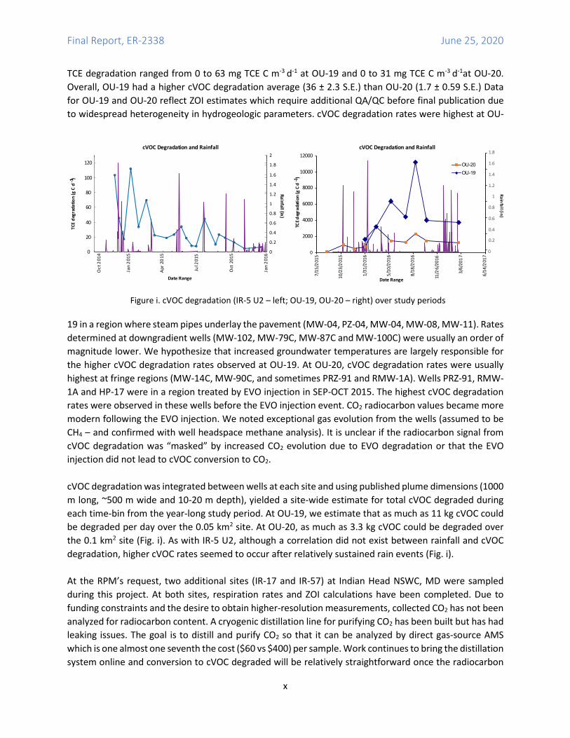
Results and Discussion At each site, time-point and well, respiration and 14CO2 data were compiled and analyzed to determine cVOC degradation (as TCE carbon degraded m-3 d-1). cVOC degradation rates were calculated for IR-5 U2, OU-19 and OU-20 at NASNI over the course of one year (each site). Respiration values along with site hydrogeologic parameters were used to create ZOI simulations for each well and time-point sampled. Ancillary measurements (cations, pH, organic acids) were used to ensure limestone (calcium carbonate) deposits did not interfere with radiocarbon analysis. Collected CO2 was combined according to well and respiration values for radiocarbon analyses due to the cost per sample. TCE degradation ranged from 0 to 400 mg TCE C m-3 d-1 at IR-5 U2, At IR-5 U2, the highest TCE degradation occurred at the plume fringes (up and side-gradient primarily) with lower degradation rates observed within the central plume with highest cVOC concentrations. At downgradient wells (e.g. MW-32, MW-35, MW-41), respiration was in line with other fringe wells (e.g. MW-21, MW-42, MW-38) but CO2 radiocarbon content often did not indicate high cVOC degradation. This was likely due to either lack of cVOC substrate(s) due to attenuation upgradient, or perhaps lack of suitable co-metabolic precursors needed for complete cVOC respiration. Site-wide cVOC degradation was computed using interpolation between sampled wells and published plume dimensions. Site-wide degradation ranged from ~4 to 112 g TCE C d-1 over the greater than one-year sampling period. Although a significant correlation did not exist, highest cVOC degradation occurred after steady rain events (Fig. i) which we hypothesize may be responsible for replenishing limiting resources and liberating pools of DNAPL from soils within the vadose zone. Time-averaged degradation over the course of the one-year collection period amounted to ~ 7 kg cVOC degraded per year.
Final Report, ER-2338 June 25, 2020
x
TCE degradation ranged from 0 to 63 mg TCE C m-3 d-1 at OU-19 and 0 to 31 mg TCE C m-3 d-1at OU-20. Overall, OU-19 had a higher cVOC degradation average (36 ± 2.3 S.E.) than OU-20 (1.7 ± 0.59 S.E.) Data for OU-19 and OU-20 reflect ZOI estimates which require additional QA/QC before final publication due to widespread heterogeneity in hydrogeologic parameters. cVOC degradation rates were highest at OU-
19 in a region where steam pipes underlay the pavement (MW-04, PZ-04, MW-04, MW-08, MW-11). Rates determined at downgradient wells (MW-102, MW-79C, MW-87C and MW-100C) were usually an order of magnitude lower. We hypothesize that increased groundwater temperatures are largely responsible for the higher cVOC degradation rates observed at OU-19. At OU-20, cVOC degradation rates were usually highest at fringe regions (MW-14C, MW-90C, and sometimes PRZ-91 and RMW-1A). Wells PRZ-91, RMW-1A and HP-17 were in a region treated by EVO injection in SEP-OCT 2015. The highest cVOC degradation rates were observed in these wells before the EVO injection event. CO2 radiocarbon values became more modern following the EVO injection. We noted exceptional gas evolution from the wells (assumed to be CH4 – and confirmed with well headspace methane analysis). It is unclear if the radiocarbon signal from cVOC degradation was “masked” by increased CO2 evolution due to EVO degradation or that the EVO injection did not lead to cVOC conversion to CO2. cVOC degradation was integrated between wells at each site and using published plume dimensions (1000 m long, ~500 m wide and 10-20 m depth), yielded a site-wide estimate for total cVOC degraded during each time-bin from the year-long study period. At OU-19, we estimate that as much as 11 kg cVOC could be degraded per day over the 0.05 km2 site. At OU-20, as much as 3.3 kg cVOC could be degraded over the 0.1 km2 site (Fig. i). As with IR-5 U2, although a correlation did not exist between rainfall and cVOC degradation, higher cVOC rates seemed to occur after relatively sustained rain events (Fig. i). At the RPM’s request, two additional sites (IR-17 and IR-57) at Indian Head NSWC, MD were sampled during this project. At both sites, respiration rates and ZOI calculations have been completed. Due to funding constraints and the desire to obtain higher-resolution measurements, collected CO2 has not been analyzed for radiocarbon content. A cryogenic distillation line for purifying CO2 has been built but has had leaking issues. The goal is to distill and purify CO2 so that it can be analyzed by direct gas-source AMS which is one almost one seventh the cost ($60 vs $400) per sample. Work continues to bring the distillation system online and conversion to cVOC degraded will be relatively straightforward once the radiocarbon
Figure i. cVOC degradation (IR-5 U2 – left; OU-19, OU-20 – right) over study periods
Date Range
0
2000
4000
6000
8000
10000
12000
7/15
/201
5
10/2
3/20
15
1/31
/201
6
5/10
/201
6
8/18
/201
6
11/2
6/20
16
3/6/
2017
6/14
/201
7
TCE
Rainfall (in)
degr
adat
ion
(gC
d-1 )
OU-20OU-19
0
0.2
0.4
0.6
0.8
1
1.2
1.4
1.6
1.8
TCE
Rainfall (in)
de
grad
atio
n
(g
C
d-1 )
Date Range
cVOC Degradation and Rainfall cVOC Degradation and Rainfall
Oct
201
4
Jan
2015
Apr 2
015
Jul 2
015
Oct
201
5
Jan
2016
0
20
40
60
80
100
120
0
0.2
0.4
0.6
0.8
1
1.2
1.4
1.6
1.8
2
Final Report, ER-2338 June 25, 2020
xi
values are obtained. Logistics for completing the datasets for these sites and eventual publication of results have been secured.
Implications for Future Research and Benefits With costs far outpacing resources available for site assessment and cleanup, robust tools to evaluate MNA and engineered solutions are necessary. We have developed technologies which target the contaminant carbon backbone and thus are able to measure contaminant degradation with certainty (radiocarbon-depleted CO2 must come from a petroleum-sourced material). The technologies can be deployed using several modes each having different suitability based on site characteristics (active trapping, passive trapping and even short-term incubations – see publications section). Well-studied sites may have ample data such that models (BioChlor and/or REMChlor) may provide adequate site management information with minimal CO2 radiocarbon evidence. For instance, it may be enough just to measure groundwater CO2 for 14C-depletion and thus irrefutably confirm a contaminant source. Sites with varying characteristics and needs will require varying degrees of coupled flux-radiocarbon evidence based on physical layout, existing data, ROD requirements, RPM needs, etc. In all cases, radiocarbon-based technologies provide concrete evidence (should 14C-depleted CO2 be associated with a contaminant plume) that contaminants are being converted to CO2 – a harmless end-product. While costly in terms of analysis costs, radiocarbon-based measurements are definitive and if well-administered can be used in place of many indirect measurements whose costs add up – and that only provide lines of evidence for contaminant respiration.
During this SERDP project, several ancillary studies were performed using commercially-available soil:atmosphere CO2 traps and using short-term respiration measurements (incubations) coupled to radiocarbon measurements to estimate cVOC degradation rates. In addition, a REMChlor model was developed for one site and methods were directly compared. This cross-validation study is in final editing for publication but very briefly, we found reasonable agreement between soil:atmosphere CO2 traps and in-well traps for a shallow cVOC DNAPL plume within a short-term deployment (~2 weeks). A long-term REMChlor model showed lower degradation rates, but results from a year-long radiocarbon-based collection demonstrated an almost 1 order of magnitude variation in rates over the course of one year. Essentially, at lower resolution (yearly timeframes), a REMChlor-type model may predict long-term cVOC attenuation. Radiocarbon-based technologies are able to provide short-term, high-resolution (seasonal) and spatial information to better refine remediation management.
Results from this SERDP project have been transitioned to ESTCP in which we will deploy various radiocarbon-based technologies at the same sites over the same timescales in order to cross validate radiocarbon techniques and assess their strengths and weaknesses given different site conditions, deployed remediation technologies and remedial management goals. The goal is to create a decision support tool (DST) encompassing these disparate but related characteristics

Final Report, ER-2338 June 25, 2020
xii
with the ultimate goal to decrease overall uncertainty and increase cost effectiveness and cost avoidance.
Final Report, ER-2338 June 25, 2020
1
Objective This project's objective is to sample existing groundwater wells to combine CO2 respiration, CO2 radiocarbon content and a Zone of Influence (ZOI) model to calculate chlorinated hydrocarbon degradation. Radiocarbon content is used to determine the fraction of petroleum-derived carbon in respired CO2. To determine cVOC degradation rate, CO2 production rate is measured by circulating groundwater well headspace through a CO2 trap over time or by passive traps deployed within a well’s headspace. A well zone of influence (ZOI) will be calculated using process-based gas transport simulation models for porous media (4). CO2 production rates and ZOI volume outputs will be used to determine CO2 respiration in a given volume associated with each groundwater monitoring well. Collected respiration CO2 will be analyzed for radiocarbon content with the understanding that 14C-depleted CO2 must arise from a fossil source (e.g. petroleum-derived fuels or industrial chemicals). The fraction CO2 derived from petroleum-source can be calculated using a two end-member model with a background sample as an index for the radiocarbon age of natural organic matter on-site. Armed with these data, the contaminant degradation rate can be determined in both temporal and spatial scales.
Ultimately, the objective is to determine
• Is remediation occurring? We will be able to track the amount (percentage basis) of the degradation end product (CO2). On the basis of this one measurement, a site manager will be able to definitively state whether (bio)degradation is occurring or not.
• At what rate is the remediation occurring? By measuring the proportion of fossil fuel-derived CO2 and the CO2 production rate over time, we will be able to calculate the rate of (bio)degradation occurring on-site. Using groundwater transport models and given an estimated size or volume of source material and plume dimensions, a much more accurate estimation of the time for remediation can be predicted:
The objective will be met by a series of field samplings at cVOC-contaminated DoD sites. Sites will be selected based on cVOC contamination, historical data already available for cVOC distribution and concentrations, hydrogeologic parameters for creating ZOI models, and RPM need/desire to host the project. Additionally, sites with existing groundwater monitoring well networks will be selected so that CO2 traps can be immediately deployed. cVOC degradation data will be scaled over the site and over the nominal one-year site collection to estimate the site-wide degradation over scalable time periods.
Final Report, ER-2338 June 25, 2020
2
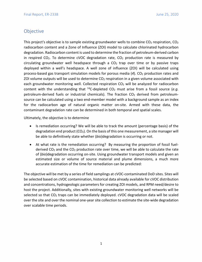
Background Environmental management and cleanup from historical contamination amounts to billions of dollars in costs. Treatment strategies such as monitored natural attenuation (MNA), enhanced passive remediation (EPR) or low cost engineered solutions can be attractive to reach Response Complete (RC) status in the United States. Many common contaminants (e.g. fuels, solvents, chlorinated compounds, munitions, etc.) are persistent and degraded slowly in the environment. Some contaminants, while readily degraded, are present in quantities too high to be degraded within reasonable time-frames. In the U.S. the Department of Defense (DoD), Department of Energy (DOE) and the Environmental Protection Agency (EPA) suggest collecting data from multiple lines of evidence to confirm contaminant attenuation and improve our estimates for remediation time-frames (2, 3). Generally, no single analysis or ex situ laboratory test provides ample evidence for in situ contaminant attenuation - and rarely can an accurate contaminant turnover rate be calculated with confidence using lines of evidence approaches (1, 7-9). Because site managers must balance risk, costs and outcomes that satisfy regulators and stakeholders, there is a persistent need for methodological improvements to provide contaminant degradation rates with increased veracity which reduces the need and expense for measuring multiple indirect lines of evidence. Recently, SERDP-funded research on radiocarbon isotope measurements has quantified organic contaminant turnover in chlorinated solvent sites. CO2 radiocarbon analysis (e.g., chlorinated hydrocarbon degradation end-product) targets the actual contaminant carbon backbone thus reducing uncertainty inherent in indirect measurements. Radiocarbon is produced in the atmosphere via cosmic radiation - converting 14N to 14C. Plants assimilate radiocarbon by photosynthesis into their tissues. When plant material becomes buried and removed from contemporary carbon cycling (e.g. during diagenesis into petroleum reserves), the 14C will decay away (~6,000-year half-life) without replacement leaving a carbon pool
(petroleum) completely devoid of any 14C. If the petroleum-based chemical leaks into the environment - and is degraded to CO2, one might expect the CO2 age upgradient of the spill to represent the natural organic matter radiocarbon age, while above an actively-degrading plume, the CO2 age would represent the fossil
Figure 1. CO2 radiocarbon age upgradient, above, and downgradient of petroleum-based chemical plume.
Final Report, ER-2338 June 25, 2020
3
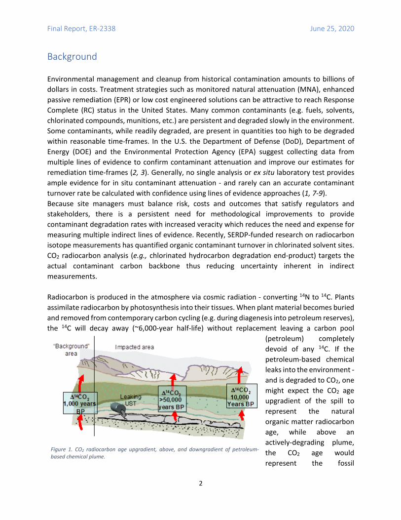
petroleum source. Downgradient, one might expect to find a mix of natural and petroleum-derived CO2 (Fig. 1). Using natural abundance 14C in the field is analogous to a laboratory microcosm with the labeled tracer "reversed”: a typical microcosm has un-labeled natural organic matter (NOM) from the water sample for instance - and 14C -labeled contaminant tracer (e.g., TCE). A natural on-site "lab" has 14C -labeled NOM (modern), and un-labeled (fossil) contaminant tracer (Fig. 2). Radiocarbon analysis can provide definitive in situ chlorinated solvent degradation evidence (or any fossil fuel-derived contaminant of interest - COI) in an accurate and cost-effective manner. Several well-chosen samples may be sufficient to confirm contaminant degradation. 14C measurements are sensitive and high resolution and able to apportion the original contaminant source, putative daughter products, and degradation end products such as CO2 and CH4 to either the natural or fossil end-member. Groundwater CO2 radiocarbon measurements have traditionally been used to assess aquifer water residence times. In the mid-1980s, highly 14C-depleted CO2 led to the discovery of sub-surface contamination and offered insight into using radiocarbon to track contaminant degradation (10). Additional studies validated this observation (11). Relying on the fact that fuels and industrial chemicals made from petroleum feedstocks are devoid of 14C, sites with subsurface fuel and chlorinated solvent contamination were systematically assessed for 14C -depleted CO2. This information was used to confirm in situ contaminant degradation rates (12-20). Most recently, CO2 radiocarbon measurements have been combined with CO2 flux estimates to determine the in situ contaminant biodegradation rate using in-well CO2 trapping, soil:atmosphere flux traps and short-term respiration incubations (16, 17, 21-25). Most applications are for LNAPL, for which the technologies are used to determine natural source-zone depletion. Application of this technology to chlorinated DNAPL sites is relatively new. Radiocarbon analysis measures the petroleum-sourced fraction in the CO2 pool. To determine COI degradation rate, CO2 production rate can be measured by atmosphere:soil traps (22), in-well CO2 traps (16, 17), or by short-term respiration incubations (21). For in-well traps, a well zone of influence (ZOI) can be calculated using process-based simulation models of gas transport in porous media (16, 17). The ZOI model and CO2 production rate are used to determine the overall CO2 production rate per soil volume. For atmosphere:soils traps, a plume depth can be assumed for converting flux per unit area to flux per unit volume. With short-term incubations,
14C-labeled TCE
14C-labeled NOM14C-free TCE
14C-free NOM
14CO2
14C-free CO2
CO2
trap
NaturalLab
LabMicrocosm
Figure 2. 14C Analysis in a "Natural Lab"
Final Report, ER-2338 June 25, 2020
4
a volumetric estimate is inherent as respiration rates are measured in a given volume under in situ conditions (21). Under all method variants, the contaminant degradation rate can be determined over both time and space. Note that biodegradation pathways of chlorinated solvents are more complicated than those at fuel hydrocarbon sites. The radiocarbon analysis approach using CO2 as a dead-end product addresses the source of the carbon (i.e., from the fossil fuel contaminant, differentiating it from modern carbon, relatively rich in 14C). However, information about the degradation pathways is not provided by this analysis. At petroleum sites, all of the 14C -depleted CO2 comes from the biodegradation of LNAPL and its dissolution products. At chlorinated solvent sites, another electron donor is biodegraded to form dissolved hydrogen which is then utilized by dechlorinating bacteria to reductively dechlorinate the solvents. At many or perhaps most of these sites, the electron donor is another anthropogenic hydrocarbon such as mineral oils or fuel compounds. These hydrocarbons also produce 14C-depleted CO2 that will be measured by the field methods implemented by this project. To account for this possible reaction, additional field parameters such as volatile fatty acids, total organic carbon, and total petroleum hydrocarbons will be measured at strategic locations to help understand the relative contribution of any anthropogenic hydrocarbon electron donor and the biodegradation of the chlorinated solvents themselves. As stated, the power of these measurements is that one analysis provides direct evidence, more straightforward and less uncertain than using an analysis suite providing indirect lines of evidence. The methods to be validated here collect respired CO2 over time and use the collected CO2 for radiocarbon analysis (providing both flux and percent of contaminant carbon) as the basis to estimate contaminant mass losses per volume. The techniques have demonstrated biodegradation in the field with analytical certainty (13-15, 17, 19, 23, 26). For the CO2 traps, using a capture diameter of 4” and a deployment time of 2 weeks, a sensitivity of 0.1% g CO2 g-1 sorbent translates into a flux detection limit of 0.025 micromoles CO2 m-2 sec-1. This can be increased by increasing capture area and deployment time, if necessary. To tie discreet lines of evidence together, an industry-standard model is often used to estimate contaminant removal. For chlorinated hydrocarbon–contaminated sites one such method is the REMChlor model. REMChlor relies on hydrogeologic data, long-term contaminant and contaminant daughter product monitoring, and other indirect data to predict contaminant degradation rate (27). REMChlor applicability may be limited if the site is relatively “new” without a full or long-term monitoring dataset. REMChlor is integrative, offering a site-wide estimate for contaminant fate and transport. It makes a good framework for evaluating radiocarbon method efficacy and cross-validation. It will be used at test sites as a foundation for inter-comparing radiocarbon methods.
Final Report, ER-2338 June 25, 2020
5
Isotope techniques have been applied to contaminated sites since the early 1990s. Although stable carbon isotope analysis has proven useful for discreet spills where a pool of starting material with known isotopic composition can be tracked (c.f., (9, 28, 29)), radiocarbon techniques track the radioactive isotope (14C) which is essentially unimpacted by physical and chemical processes (half-live is an accepted standard). Several variations on combining radiocarbon and CO2 flux studies have been developed relying on measuring CO2 flux and radiocarbon from the same subsample(s). One technology involves passive CO2 flux traps (22). Although recently commercialized (E-Flux, LLC), this is a mature technology that relies on open cartridges containing CO2 adsorbent material deployed across the soil:atmosphere interface. The trap design eliminates ambient CO2 interference. The traps are deployed for multiple days (typically several weeks), recovered, the CO2 quantified, then subjected to radiocarbon analysis. 14C-depleted CO2 (relative to uncontaminated background sites) can be related to contaminant degradation over the sampled area (mg contaminant CO2 m-2 d-1). This technology has been used at hundreds of LNAPL contaminated sites, having achieved significant regulatory acceptance. This is the only mature technology to measure natural source-zone depletion rates that routinely accounts for carbon isotopic correction (30).
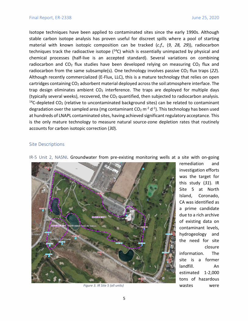
Site Descriptions IR-5 Unit 2, NASNI. Groundwater from pre-existing monitoring wells at a site with on-going
remediation and investigation efforts was the target for this study (31). IR Site 5 at North Island, Coronado, CA was identified as a prime candidate due to a rich archive of existing data on contaminant levels, hydrogeology and the need for site
closure information. The site is a former landfill. An estimated 1-2,000 tons of hazardous wastes were Figure 3. IR Site 5 (all units)
Final Report, ER-2338 June 25, 2020
6
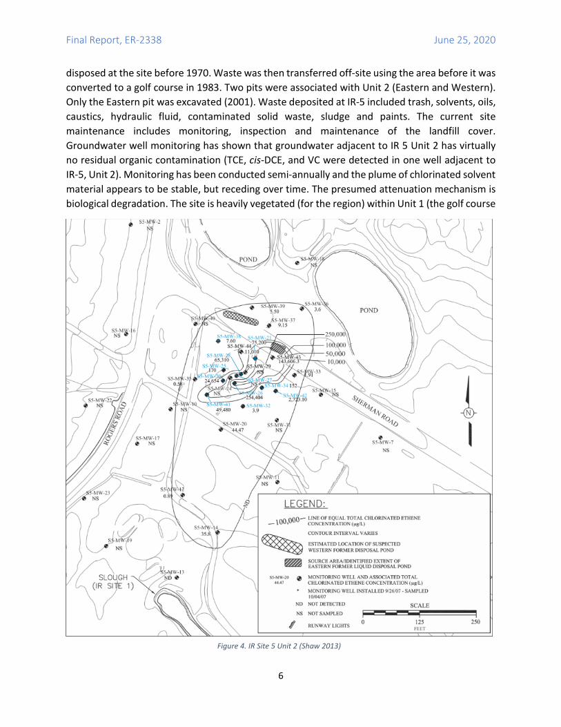
disposed at the site before 1970. Waste was then transferred off-site using the area before it was converted to a golf course in 1983. Two pits were associated with Unit 2 (Eastern and Western). Only the Eastern pit was excavated (2001). Waste deposited at IR-5 included trash, solvents, oils, caustics, hydraulic fluid, contaminated solid waste, sludge and paints. The current site maintenance includes monitoring, inspection and maintenance of the landfill cover. Groundwater well monitoring has shown that groundwater adjacent to IR 5 Unit 2 has virtually no residual organic contamination (TCE, cis-DCE, and VC were detected in one well adjacent to IR-5, Unit 2). Monitoring has been conducted semi-annually and the plume of chlorinated solvent material appears to be stable, but receding over time. The presumed attenuation mechanism is biological degradation. The site is heavily vegetated (for the region) within Unit 1 (the golf course
Figure 4. IR Site 5 Unit 2 (Shaw 2013)
Final Report, ER-2338 June 25, 2020
7
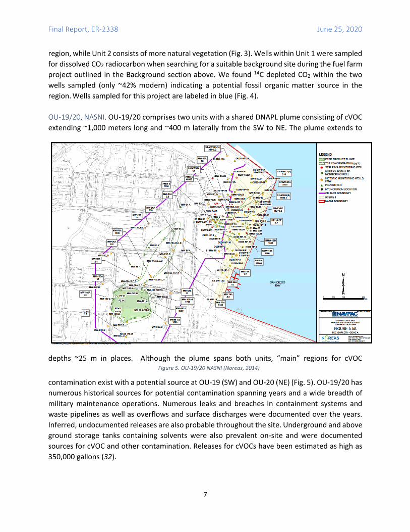
region, while Unit 2 consists of more natural vegetation (Fig. 3). Wells within Unit 1 were sampled for dissolved CO2 radiocarbon when searching for a suitable background site during the fuel farm project outlined in the Background section above. We found 14C depleted CO2 within the two wells sampled (only ~42% modern) indicating a potential fossil organic matter source in the region. Wells sampled for this project are labeled in blue (Fig. 4). OU-19/20, NASNI. OU-19/20 comprises two units with a shared DNAPL plume consisting of cVOC extending ~1,000 meters long and ~400 m laterally from the SW to NE. The plume extends to
depths ~25 m in places. Although the plume spans both units, “main” regions for cVOC
contamination exist with a potential source at OU-19 (SW) and OU-20 (NE) (Fig. 5). OU-19/20 has numerous historical sources for potential contamination spanning years and a wide breadth of military maintenance operations. Numerous leaks and breaches in containment systems and waste pipelines as well as overflows and surface discharges were documented over the years. Inferred, undocumented releases are also probable throughout the site. Underground and above ground storage tanks containing solvents were also prevalent on-site and were documented sources for cVOC and other contamination. Releases for cVOCs have been estimated as high as 350,000 gallons (32).
Figure 5. OU-19/20 NASNI (Noreas, 2014)
Final Report, ER-2338 June 25, 2020
8
NASNI soil is mostly comprised of sands, silts, and very small amounts of clay (from mainland deposits). Much of the perimeter is derived from dredge material used to grade the island – a process begun in the 1930s. This fill is primarily poorly-graded sands and silty sands. Groundwater is not used for drinking water and a shallow aquifer (home to the impacts) exists ~1-8m below ground surface. Groundwater flow at the site is towards the NE and discharges into San Diego Bay. Four main zones (A-D) have been identified from the soil surface to ~25 m below ground surface (32). Groundwater level measurements and slug tests provided standard hydrogeologic information for various zones on site. Vary small gradients exist across the site (0.001 to 0.002 ft ft-1). However, due to variations in soil types (natural vs fill), a very large range in aquifer transmissivity values is found (0.5 up to ~1,000 ft2 min-1). Tidal influence is relatively small (up to 30%) at shallow groundwater wells, but may be over 50% at deeper wells. Most influence is below ~20 meters where salinity has been recorded at 30 (32).
Due to remedial investigations begun in the 1990s, LNAPL (consisting of mostly JP-5 and Staddard solvent) and DNAPL (cVOC) plumes were delineated. CERCLA activities began in the 1990s with LNAPL recovery. Various LNAPL recovery efforts led to removal of ~17,000 gallons LNAPL bringing dissolved concentrations down to remediation goals. DNAPL has been persistent and several pilot studies using zero valent iron (ZVI), persulfate, and EVO injection were used to evaluate remedial
alternatives. Current values for fuel-related LNAPL components are low across OU-19/20 with
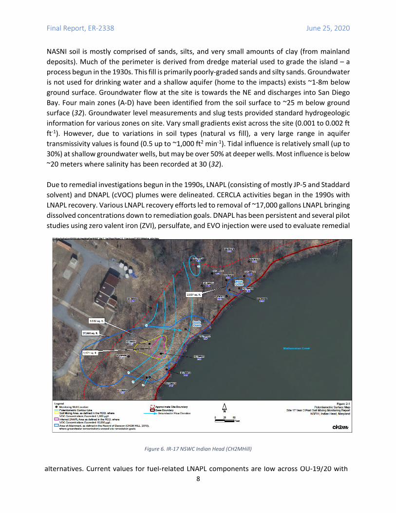
Figure 6. IR-17 NSWC Indian Head (CH2MHill)
Final Report, ER-2338 June 25, 2020
9
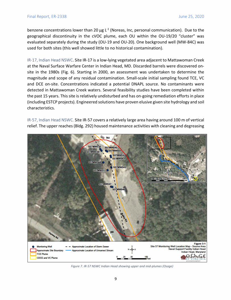
benzene concentrations lower than 20 µg L-1 (Noreas, Inc, personal communication). Due to the geographical discontinuity in the cVOC plume, each OU within the OU-19/20 “cluster” was evaluated separately during the study (OU-19 and OU-20). One background well (MW-84C) was used for both sites (this well showed little to no historical contamination). IR-17, Indian Head NSWC. Site IR-17 is a low-lying vegetated area adjacent to Mattawoman Creek at the Naval Surface Warfare Center in Indian Head, MD. Discarded barrels were discovered on-site in the 1980s (Fig. 6). Starting in 2000, an assessment was undertaken to determine the magnitude and scope of any residual contamination. Small-scale initial sampling found TCE, VC and DCE on-site. Concentrations indicated a potential DNAPL source. No contaminants were detected in Mattawoman Creek waters. Several feasibility studies have been completed within the past 15 years. This site is relatively undisturbed and has on-going remediation efforts in place (including ESTCP projects). Engineered solutions have proven elusive given site hydrology and soil characteristics. IR-57, Indian Head NSWC. Site IR-57 covers a relatively large area having around 100 m of vertical relief. The upper reaches (Bldg. 292) housed maintenance activities with cleaning and degreasing
Figure 7. IR-57 NSWC Indian Head showing upper and mid-plumes (Osage)
Final Report, ER-2338 June 25, 2020
10
operations during the 1970s and 1980s. Operations ceased in 1989. TCE was used, stored and reclaimed using barrels on-site. Leaking during operations is thought responsible for TCE, VC and DCE contamination in soils and groundwater on-site. The site was treated with a proton reduction technology (PRT) consisting of electrodes designed to create reducing conditions on-site for reductive dechlorination. In a 2013 report, the initial test demonstrated reducing conditions at selected wells - but no concomitant decrease in TCE concentrations.
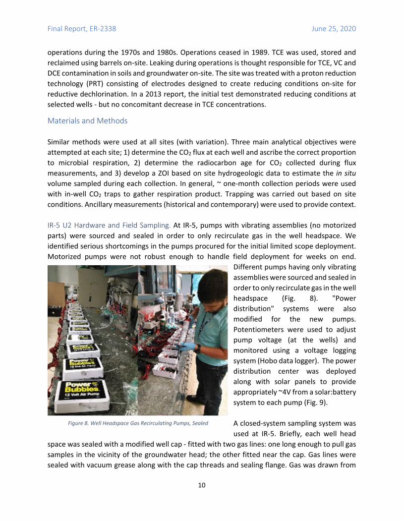
Materials and Methods Similar methods were used at all sites (with variation). Three main analytical objectives were attempted at each site; 1) determine the CO2 flux at each well and ascribe the correct proportion to microbial respiration, 2) determine the radiocarbon age for CO2 collected during flux measurements, and 3) develop a ZOI based on site hydrogeologic data to estimate the in situ volume sampled during each collection. In general, ~ one-month collection periods were used with in-well CO2 traps to gather respiration product. Trapping was carried out based on site conditions. Ancillary measurements (historical and contemporary) were used to provide context. IR-5 U2 Hardware and Field Sampling. At IR-5, pumps with vibrating assemblies (no motorized parts) were sourced and sealed in order to only recirculate gas in the well headspace. We identified serious shortcomings in the pumps procured for the initial limited scope deployment. Motorized pumps were not robust enough to handle field deployment for weeks on end.
Different pumps having only vibrating assemblies were sourced and sealed in order to only recirculate gas in the well headspace (Fig. 8). "Power distribution" systems were also modified for the new pumps. Potentiometers were used to adjust pump voltage (at the wells) and monitored using a voltage logging system (Hobo data logger). The power distribution center was deployed along with solar panels to provide appropriately ~4V from a solar:battery system to each pump (Fig. 9). A closed-system sampling system was used at IR-5. Briefly, each well head
space was sealed with a modified well cap - fitted with two gas lines: one long enough to pull gas samples in the vicinity of the groundwater head; the other fitted near the cap. Gas lines were sealed with vacuum grease along with the cap threads and sealing flange. Gas was drawn from
Figure 8. Well Headspace Gas Recirculating Pumps, Sealed
Final Report, ER-2338 June 25, 2020
11
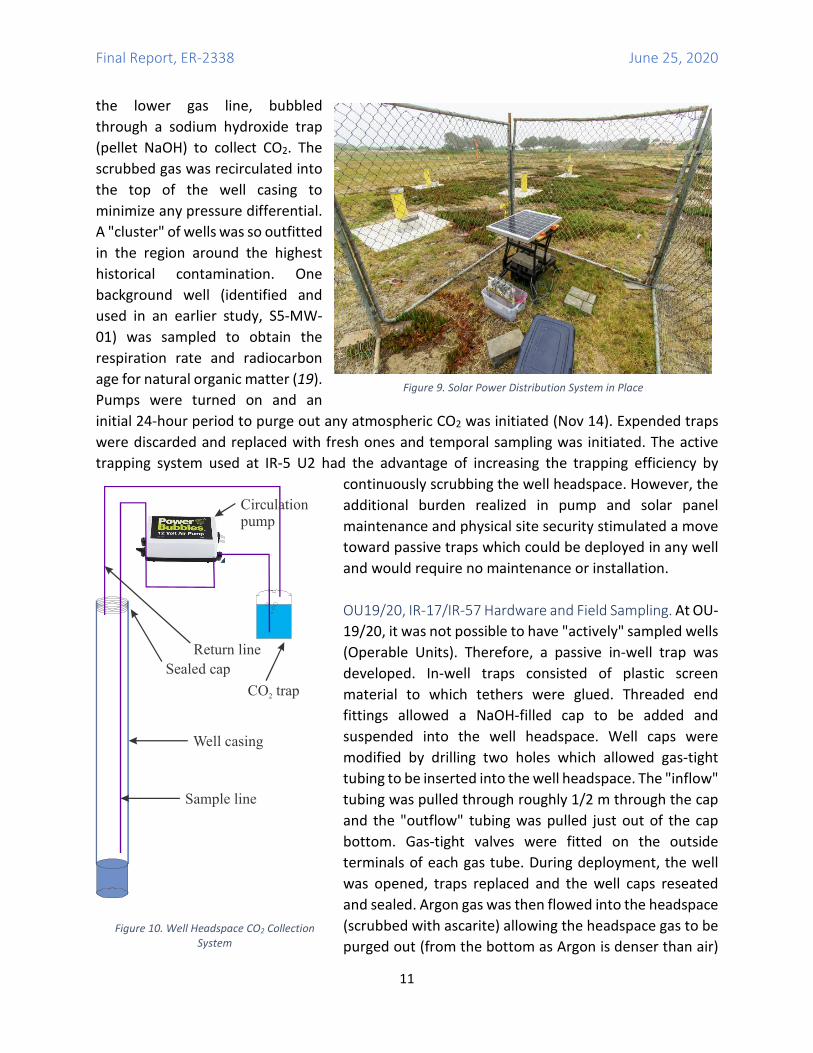
the lower gas line, bubbled through a sodium hydroxide trap (pellet NaOH) to collect CO2. The scrubbed gas was recirculated into the top of the well casing to minimize any pressure differential. A "cluster" of wells was so outfitted in the region around the highest historical contamination. One background well (identified and used in an earlier study, S5-MW-01) was sampled to obtain the respiration rate and radiocarbon age for natural organic matter (19). Pumps were turned on and an initial 24-hour period to purge out any atmospheric CO2 was initiated (Nov 14). Expended traps were discarded and replaced with fresh ones and temporal sampling was initiated. The active trapping system used at IR-5 U2 had the advantage of increasing the trapping efficiency by
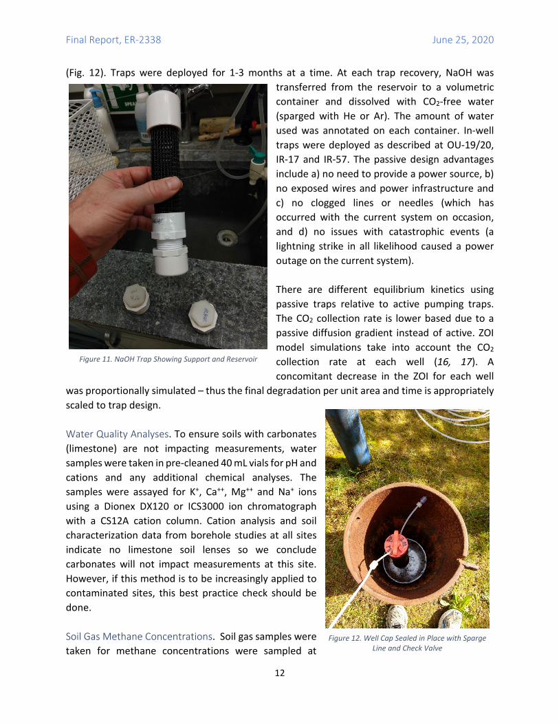
continuously scrubbing the well headspace. However, the additional burden realized in pump and solar panel maintenance and physical site security stimulated a move toward passive traps which could be deployed in any well and would require no maintenance or installation. OU19/20, IR-17/IR-57 Hardware and Field Sampling. At OU-19/20, it was not possible to have "actively" sampled wells (Operable Units). Therefore, a passive in-well trap was developed. In-well traps consisted of plastic screen material to which tethers were glued. Threaded end fittings allowed a NaOH-filled cap to be added and suspended into the well headspace. Well caps were modified by drilling two holes which allowed gas-tight tubing to be inserted into the well headspace. The "inflow" tubing was pulled through roughly 1/2 m through the cap and the "outflow" tubing was pulled just out of the cap bottom. Gas-tight valves were fitted on the outside terminals of each gas tube. During deployment, the well was opened, traps replaced and the well caps reseated and sealed. Argon gas was then flowed into the headspace (scrubbed with ascarite) allowing the headspace gas to be purged out (from the bottom as Argon is denser than air)
Figure 9. Solar Power Distribution System in Place
Figure 10. Well Headspace CO2 Collection System
Return lineSealed cap
CO trap2
Sample line
Well casing
Circulationpump
Final Report, ER-2338 June 25, 2020
12
(Fig. 12). Traps were deployed for 1-3 months at a time. At each trap recovery, NaOH was transferred from the reservoir to a volumetric container and dissolved with CO2-free water (sparged with He or Ar). The amount of water used was annotated on each container. In-well traps were deployed as described at OU-19/20, IR-17 and IR-57. The passive design advantages include a) no need to provide a power source, b) no exposed wires and power infrastructure and c) no clogged lines or needles (which has occurred with the current system on occasion, and d) no issues with catastrophic events (a lightning strike in all likelihood caused a power outage on the current system). There are different equilibrium kinetics using passive traps relative to active pumping traps. The CO2 collection rate is lower based due to a passive diffusion gradient instead of active. ZOI model simulations take into account the CO2 collection rate at each well (16, 17). A concomitant decrease in the ZOI for each well
was proportionally simulated – thus the final degradation per unit area and time is appropriately scaled to trap design. Water Quality Analyses. To ensure soils with carbonates (limestone) are not impacting measurements, water samples were taken in pre-cleaned 40 mL vials for pH and cations and any additional chemical analyses. The samples were assayed for K+, Ca++, Mg++ and Na+ ions using a Dionex DX120 or ICS3000 ion chromatograph with a CS12A cation column. Cation analysis and soil characterization data from borehole studies at all sites indicate no limestone soil lenses so we conclude carbonates will not impact measurements at this site. However, if this method is to be increasingly applied to contaminated sites, this best practice check should be done. Soil Gas Methane Concentrations. Soil gas samples were taken for methane concentrations were sampled at
Figure 12. Well Cap Sealed in Place with Sparge Line and Check Valve
Figure 11. NaOH Trap Showing Support and Reservoir
Final Report, ER-2338 June 25, 2020
13
various time-points since November 2014. Samples were taken from NaOH gas trap lines (Fig. 12) during trap replacement (while pumps were not operational) or before well headspace was compromised prior to trap removal and replacement. Headspace gas was sampled by 60 mL syringe fitted with a three-way valve. Two samples were pulled and discarded. The third sample was reserved. The sample was transferred underwater to a water-filled inverted serum bottle (displacing the water). A gas-impermeable septum was inserted and the bottle was crimp-sealed. Serum bottles were returned to NRL. A subsample from the bottle headspace (3 mL) was injected into a Shimadzu GC-14A gas chromatograph fitted with a Hayesep 0.80/100 column. Column flow was ~10 mL min-1 and concentrations were determined against certified reference standards (Scott Gas, Plumbsteadville, PA). Radiocarbon Analysis. Water samples with ample dissolved inorganic carbon (e.g. CO2) were sent to the University of Georgia Center for Applied Isotope Studies (CIAS). CAIS sparges, cryogenically distils, and purifies CO2 then produces graphite targets for accelerator mass spectrometry (AMS). The high-sensitivity analysis allows radiocarbon age dating in samples back to ~50,000 years. Due to the high per-sample costs, samples were combined quantitatively to decease the number of total analyses. Details are given in the supplementary materials. Data are reported in percent modern carbon (pmc) which can be converted to ∆14C (per mil – ‰) for modeling (see below) using standard conversions (33). CO2 Production Rate Analysis. Collected CO2 samples (from traps) were diluted in a known amount of Ar- or He-sparged water until all residual solid NaOH was dissolved. Samples were appropriately diluted and analyzed by acidifying the CO2 out of solution and measuring by coulometry (34). CO2 was quantified relative to a certified reference material (35). CO2 production rate was calculated by the total recovered CO2 divided by the time of collection. Respiration was determined for each well by subtracting the lowest collection rate measurement (assumed to be equilibrium CO2 collection only). Zone of Influence Model/Simulation. ZOI models were created for each well based on the well hydrogeology and local soil characteristics (obtained from boring records, slug tests, conductivity tests, etc.). Input variables included well construction (casing dimensions, depth to water) temperature, atmospheric pressure and soil permeability values. Analysis of well logs and prior well tests in the project area were used to develop a hydrogeologic model of the site. This information was coupled with CO2 equilibrium simulation models to create the ZOI models. The ZOI model was developed using MT3DMS (36) and MODFLOW-2005 (37). MT3DMS is the biodegradation model capable of simulating multi-solute transport and reaction, and used to simulate CO2 solute transport as a part of the ZOI model. MODFLOW-2005 is the hydrogeological model considered as the reference code to simulate groundwater dynamics and is used to simulate groundwater flow in the unconfined aquifer at the study site. The two models have been used together as the standard package for multi-species contaminant transport simulations (38). In this study, ModelMuse was used to link and interface the two models (39).
Final Report, ER-2338 June 25, 2020
14
The target for this study was CO2 produced from chlorinated solvent degradation (e.g. TCE, DCE and VC). Among different biodegradation models studied (e.g. MT3DMS, RT3D, Biosereen, Biochlor, and SEAM3D), there is no model that is capable of coupling a groundwater simulation model and simulating this complex CO2 system while tracking individual CO2 solutes. This project treats all CO2 with different origins together - and the radiocarbon content was used to uniquely distinguish CO2 derived from chlorinated solvents. Determining the Contaminant Respired. The isotopic mixing model was applied to each sample using the radiocarbon value for CO2 collected at the background wells (MW-01 for IR-5 U2 and MW-84C for OU-19/20) as the appropriate site-wide background value (∆14Cnatural organic matter). The ∆14Cpetroleum was assigned the value -999 ‰. The fractionpetroleum was solved for each well via a two end-member mixing model:
∆14CO2 = (∆14Cpetroluem X fractionpetroleum) + [∆14Cnatural organic matter X (1 – fractionpetroluem)]
14C-content measurements could then be used to determine the proportion of vadose zone CO2 derived from the cVOC (15). Using respiration values (g CO2 produced per unit time) and ZOI simulations for each time-point and well (volume sampled), contaminant degraded per unit time and volume can be computed in a straightforward manner (e.g. CO2 respired per unit time times the fraction derived from fossil sources divided by the volume sampled).
Final Report, ER-2338 June 25, 2020
15
Results and Discussion Roughly one year of measurements were completed at each of two sites during the course of the project. At the RPM’s request, we initiated measurements at two sites local to NRL (IR-17 and IR-57, Indian Head NSWC). These sites were sampled for all parameters but radiocarbon analysis has not been completed due to time and funding constraints. Site-specific results and discussion follow: IR-5 Unit 2. Traps were deployed starting in November 2014 and cycled every 2-4 weeks until November 2015. Trap material was analyzed for CO2 concentration and radiocarbon. Selected concurrent samples for cations, well casing CH4 concentrations and water quality measurements were taken. Results are summarized by analysis. ZOI Simulations. Groundwater hydraulic and CO2 solute properties for the study site were obtained from previous reports (40, 41). Three years of weather data (2007, 2011 and 2012) were obtained from the CIMIS San Diego station (Station ID 184) to estimate the recharge rate of the aquifer. Tidal data for the same three years were obtained from the NOAA San Diego Station (Station ID: 9410170) to define boundary conditions. From the aerial photo, surface water pools (e.g. ponds and creeks) were identified on the Northeastern side of the area (in the golf course and park). A constant head equal to the elevation of these surface water bodies was assigned to the boundary. The following shows results for one collection time period (in detail). Each collection time period was simulated accordingly. The areal model indicated that the effects of short term (e.g. daily and weekly periods) changes in sea level around the peninsula on groundwater flow at the study site were not significant. This result agrees with the previous report from Wiedemeier and Associates (personal communication, April, 2013). The ground-water hydrology at the study site is usually steady
between late summer and fall. Therefore, the groundwater flow during the CO2 collection periods was assumed steady (i.e. constant hydraulic gradient). The hydraulic gradient estimated by the areal model was 0.009 m m-1, which was reasonably close to the value estimated
Table 1. Hydrogeologic Parameters Used in IR-5 U2 ZOI Model(s)
Parameter Units Value
Hydrology Hydraulic Conductivity (m hr-1) 0.44 (aquifer), 10 (well) Porosity (aquifer) 0.48 (aquifer), 0.99 (well) Bulk Density (g cm-3) 1.4 Specific Yield (cm3 cm-3) 0.2 Hydraulic Gradient (m m-1) 0.015 CO2 Solute Transport Diffusion Coefficient (CO2) (m2 hr-1) 6.77 X 10⁻⁶ Longitudinal Dispersivity (m) 6.1 Horizontal Transverse Dispersivity (m) 0.61 Vertical Transverse Dispersivity (m) 0.061 Soil Gas CO2 (%) 0.56
Final Report, ER-2338 June 25, 2020
16
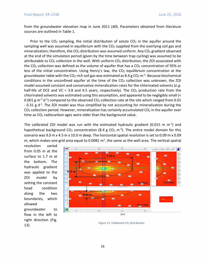
from the groundwater elevation map in June 2011 (40). Parameters obtained from literature sources are outlined in Table 1. Prior to the CO2 sampling, the initial distribution of solute CO2 in the aquifer around the sampling well was assumed in equilibrium with the CO2 supplied from the overlying soil gas and mineralization; therefore, the CO2 distribution was assumed uniform. Any CO2 gradient observed at the end of the simulation period (given by the time between trap cycling) was assumed to be attributable to CO2 collection in the well. With uniform CO2 distribution, the ZOI associated with the CO2 collection was defined as the volume of aquifer that has a CO2 concentration of 95% or less of the initial concentration. Using Henry’s law, the CO2 equilibrium concentration at the groundwater table with the CO2-rich soil gas was estimated as 8.4 g CO2 m-3. Because biochemical conditions in the unconfined aquifer at the time of the CO2 collection was unknown, the ZOI model assumed constant and conservative mineralization rates for the chlorinated solvents (e.g. half-life of DCE and VC = 3.8 and 9.5 years, respectively). The CO2 production rate from the chlorinated solvents was estimated using this assumption, and appeared to be negligibly small (< 0.001 g m-3 d-1) compared to the observed CO2 collection rate at the site which ranged from 0.01 - 0.31 g d-1. The ZOI model was thus simplified by not accounting for mineralization during the CO2 collection period. However, mineralization has certainly accumulated CO2 in the aquifer over time as CO2 radiocarbon ages were older than the background value. The calibrated ZOI model was run with the estimated hydraulic gradient (0.015 m m-1) and hypothetical background CO2 concentration (8.4 g CO2 m-3). The entire model domain for this scenario was 9.0 m x 4.5 m x 10.0 m deep. The horizontal spatial resolution is set to 0.09 m x 0.09 m, which makes one grid area equal to 0.0081 m2, the same as the well area. The vertical spatial resolution varied from 0.05 m at the surface to 1.7 m at the bottom. The hydraulic gradient was applied to the ZOI model by setting the constant head condition along the two boundaries, which allowed groundwater to flow in the left to right direction (Fig. 13).
Figure 13. Calibrated CO2 Distribution.
Final Report, ER-2338 June 25, 2020
17
Each well and time-point ZOI model was then coupled with the observed CO2 collocation rates. The calibration assumed that the collection rate was constant during the collection period. The calibration also assumed the equilibrium between the CO2 output (i.e. collection) and supply (i.e. diffusion) at the water table in the well at the end of the collection period. In other words, the CO2 concentration of the water surface in the well was assumed to be decreased to 0.0 g CO2 m-
3 by the end of the simulation.
Taking the CO2 collection rate into account, ZOI calibrations varied (see Appendix A for data from all simulations). The calibration result indicated strong linear correlations between the observed collection rate and the calibrated background CO2 concentration. Also, estimated ZOI volumes indicated a strong linear correlation with background CO2 concentrations and thus CO2 collection rates. Assuming the partial pressure of the atmospheric CO2 of 0.04 %, the equilibrium CO2 concentration of non-contaminated aquifer exposed to the atmosphere would be 0.60 g m-3. The estimated background CO2 concentration for all collection rates was higher than this value which suggests groundwater contamination with chlorinated solvents (e.g. DCE and VC) and their active mineralization. However, the estimated background CO2 concentrations were routinely below solubility of CO2 (1,450 g m-3 at 25 °C) so CO2 does not appear to be saturated in the aquifer.
The calibrations assumed a steady hydraulic gradient and constant collection rates. A supplemental simulation for the average CO2 collection rate indicated approximately 50 % increase in the estimated background CO2 concentration (i.e. increased from 6.5 to 9.7 g m-3) with 10 % increase in hydraulic gradient (i.e. increased from 0.0150 to 0.0165 m m-1). Another supplemental simulation for the average CO2 collection rate indicated approximately 46 % increase in the estimate background CO2 concentration (i.e. increased 6.5 to 9.5 g m-3) if the collection rate changed from 0.00530 (+10 %) to 0.00434 g h-1 (-10 %) over the 2-week collection period. Furthermore, the ZOI model assumed constant and conservative reaction rate for the chlorinated solvents. After accounting for the small difference in the first and second CO2 collection rates, the reaction rate appeared to be underestimated for the study site. Therefore, it is important for ZOI estimation to collect and account for these aquifer and operation parameters for better accuracy and reliability.
Water Quality Measurements. Samples for cation and pH were analyzed in March and July 2013 before trap deployment to assess site suitability. The primary concern is that low pH might promote carbonate dissolution which could bias radiocarbon analysis (see M&M section). Due to the nature of soils at NASNI, this analysis was probably not necessary (no significant source of carbonates in dredge fill), however, shell deposits could be of concern. pH was near neutral for all wells sampled (Table 2). Wells on the site's Southern side generally had a higher Na+ content, but were not in a range which indicated significant seawater intrusion. Calcium ion concentrations ranged from 8.0 to 58 mg L-1 (Tables 1 and 2) but did not inversely correlate with pH to indicate significant carbonate dissolution during either sampling (r2 < 0.3). We performed a trend analysis with the water quality data using principal components analysis (PCA). Bi-plots showed no strong loadings with any water quality variable.
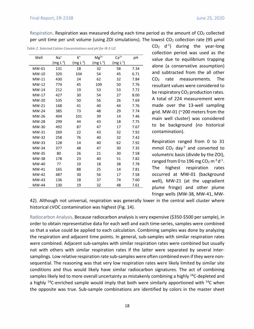
Final Report, ER-2338 June 25, 2020
18
Respiration. Respiration was measured during each time period as the amount of CO2 collected per unit time per unit volume (using ZOI simulations). The lowest CO2 collection rate (95 µmol
CO2 d-1) during the year-long collection period was used as the value due to equilibrium trapping alone (a conservative assumption) and subtracted from the all other CO2 rate measurements. The resultant values were considered to be respiratory CO2 production rates. A total of 224 measurement were made over the 13-well sampling grid. MW-01 (~200 meters from the main well cluster) was considered to be background (no historical contamination).
Respiration ranged from 0 to 31 mmol CO2 day-1 and converted to volumetric basis (divide by the ZOI), ranged from 0 to 196 mg CO2 m-3 d-1. The highest respiration rates occurred at MW-01 (background well), MW-21 (at the upgradient plume fringe) and other plume fringe wells (MW-38, MW-41, MW-
42). Although not universal, respiration was generally lower in the central well cluster where historical cVOC contamination was highest (Fig. 14).
Radiocarbon Analysis. Because radiocarbon analysis is very expensive ($350-$500 per sample), in order to obtain representative data for each well and each time-series, samples were combined so that a value could be applied to each calculation. Combining samples was done by analyzing the respiration and adjacent time points. In general, sub-samples with similar respiration rates were combined. Adjacent sub-samples with similar respiration rates were combined but usually not with others with similar respiration rates if the latter were separated by several inter-samplings. Low relative respiration rate sub-samples were often combined even if they were non-sequential. The reasoning was that very low respiration rates were likely limited by similar site conditions and thus would likely have similar radiocarbon signatures. The act of combining samples likely led to more overall uncertainty as mistakenly combining a highly 14C-depleted and a highly 14C-enriched sample would imply that both were similarly apportioned with 14C when the opposite was true. Sub-sample combinations are identified by colors in the master sheet
Table 2. Selected Cation Concentrations and pH for IR-5 U2
Well
Na+ (mg L-1)
K+ (mg L-1)
Mg2+ (mg L-1)
Ca2+ (mg L-1)
pH
MW-01 131 18 32 58 7.34 MW-10 320 104 54 45 6.71 MW-11 430 24 62 32 7.84 MW-12 774 45 109 50 7.76 MW-14 212 19 53 53 7.72 MW-17 427 30 54 27 8.00 MW-20 535 50 56 26 7.69 MW-21 168 41 40 44 7.76 MW-24 385 73 48 29 7.74 MW-26 404 101 39 14 7.46 MW-28 299 44 43 18 7.75 MW-30 492 87 47 17 7.67 MW-31 269 22 43 32 7.92 MW-32 258 76 40 32 7.42 MW-33 128 14 40 62 7.92 MW-34 377 48 47 30 7.35 MW-35 80 26 21 30 7.58 MW-38 178 23 40 51 7.82 MW-40 77 10 18 38 7.78 MW-41 165 88 25 14 7.81 MW-42 487 30 56 17 7.58 MW-43 136 18 37 74 7.60 MW-44 130 19 32 48 7.61
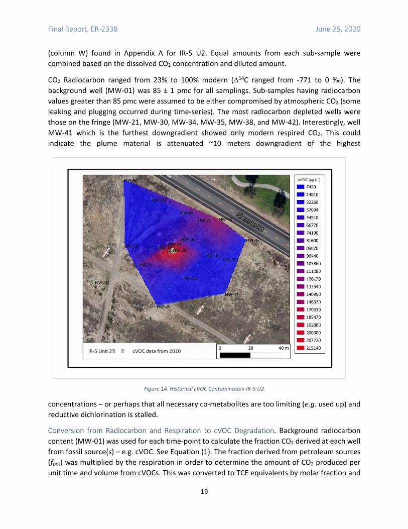
Final Report, ER-2338 June 25, 2020
19
(column W) found in Appendix A for IR-5 U2. Equal amounts from each sub-sample were combined based on the dissolved CO2 concentration and diluted amount.
CO2 Radiocarbon ranged from 23% to 100% modern (∆14C ranged from -771 to 0 ‰). The background well (MW-01) was 85 ± 1 pmc for all samplings. Sub-samples having radiocarbon values greater than 85 pmc were assumed to be either compromised by atmospheric CO2 (some leaking and plugging occurred during time-series). The most radiocarbon depleted wells were those on the fringe (MW-21, MW-30, MW-34, MW-35, MW-38, and MW-42). Interestingly, well MW-41 which is the furthest downgradient showed only modern respired CO2. This could indicate the plume material is attenuated ~10 meters downgradient of the highest
concentrations – or perhaps that all necessary co-metabolites are too limiting (e.g. used up) and reductive dichlorination is stalled.
Conversion from Radiocarbon and Respiration to cVOC Degradation. Background radiocarbon content (MW-01) was used for each time-point to calculate the fraction CO2 derived at each well from fossil source(s) – e.g. cVOC. See Equation (1). The fraction derived from petroleum sources (fpet) was multiplied by the respiration in order to determine the amount of CO2 produced per unit time and volume from cVOCs. This was converted to TCE equivalents by molar fraction and
IR-5 Unit 2 cVOC data from 2010
cVOC (µg L )-1
Figure 14. Historical cVOC Contamination IR-5 U2
Final Report, ER-2338 June 25, 2020
20
molecular weight. Thus, the amount of TCE degraded over the site was calculated (mg TCE C m-3 d-1). This calculation ranged from 0 to 400 mg C m-3 d-1 with the highest values at fringe wells (MW-21, MW-34, MW-35, MW-38 and MW42). Within the central well cluster, the only significant TCE degradation occurred at MW-26.
TCE degradation was interpolated over the site using the Matlab® scatteredInterpolant function. The relatively regularly-spaced wells justified using the ‘natural’ interpolation method and no extrapolation was used as wells having clogged lines or otherwise compromised were left out of the final spatial calculations. Interpolant outputs contained spatial area sampled (m2 gridded between sampled wells), and an interpolated degradation rate. A uniform 3 m plume depth (31) was used to estimate the total degradation over the site in terms of the plume volume. TCE (carbon basis) degradation interpolated over the site for each collection period is shown in Figs. 16-34 (images courtesy of the U.S. Geological Survey).
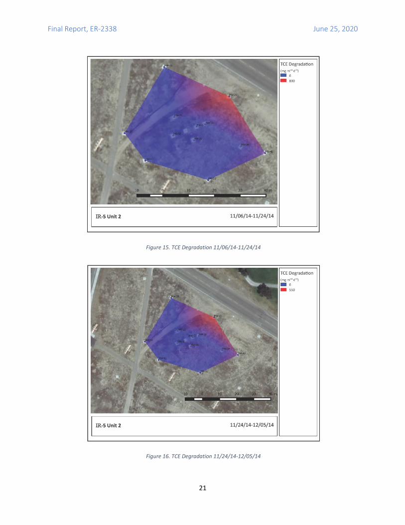
Final Report, ER-2338 June 25, 2020
21
Figure 16. TCE Degradation 11/24/14-12/05/14
Figure 15. TCE Degradation 11/06/14-11/24/14
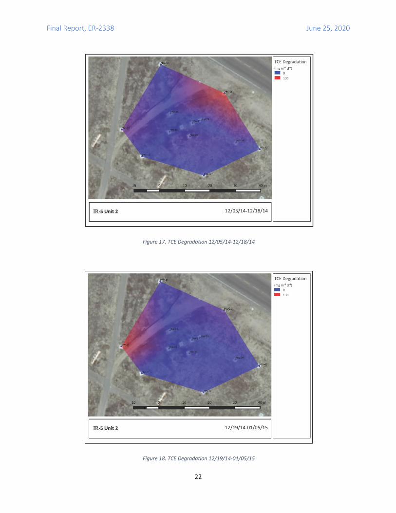
Final Report, ER-2338 June 25, 2020
22
Figure 17. TCE Degradation 12/05/14-12/18/14
Figure 18. TCE Degradation 12/19/14-01/05/15
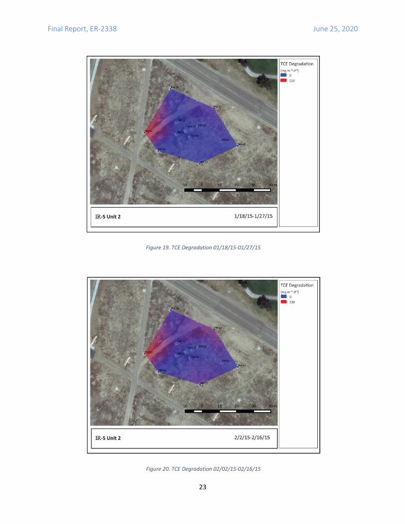
Final Report, ER-2338 June 25, 2020
23
Figure 19. TCE Degradation 01/18/15-01/27/15
Figure 20. TCE Degradation 02/02/15-02/16/15
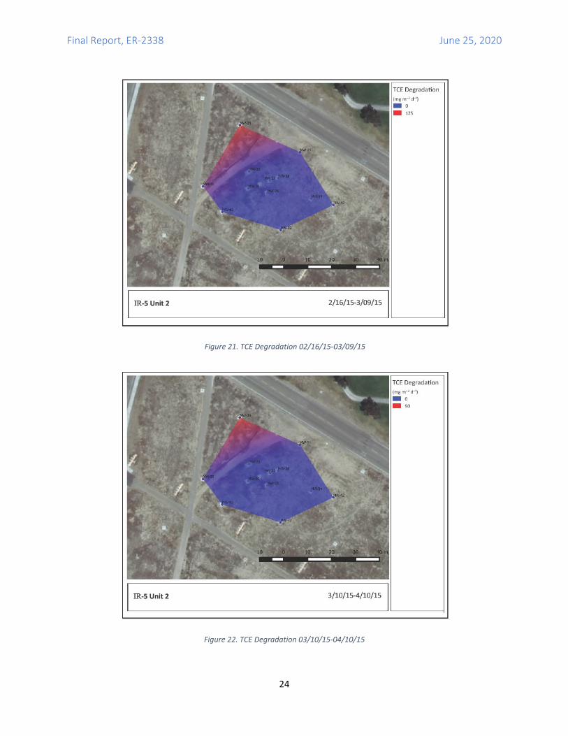
Final Report, ER-2338 June 25, 2020
24
Figure 22. TCE Degradation 03/10/15-04/10/15
Figure 21. TCE Degradation 02/16/15-03/09/15
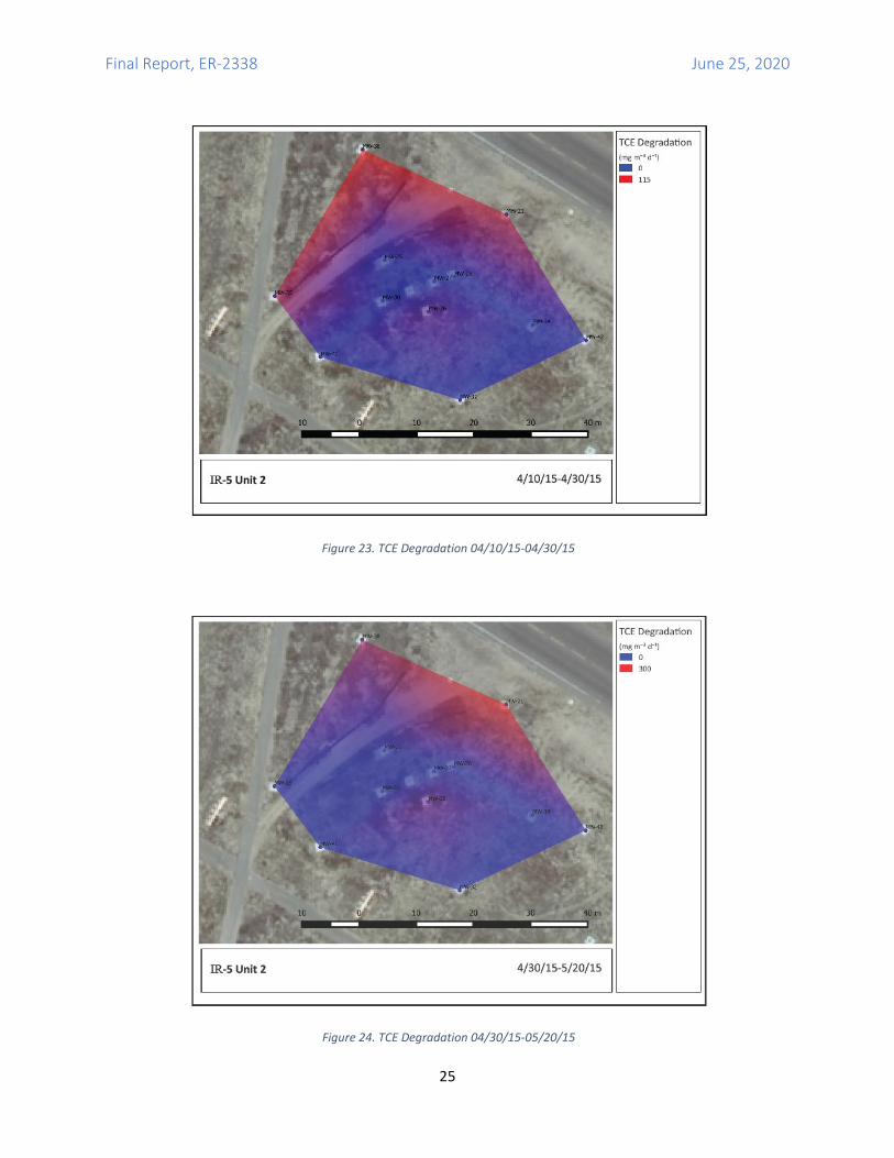
Final Report, ER-2338 June 25, 2020
25
Figure 23. TCE Degradation 04/10/15-04/30/15
Figure 24. TCE Degradation 04/30/15-05/20/15
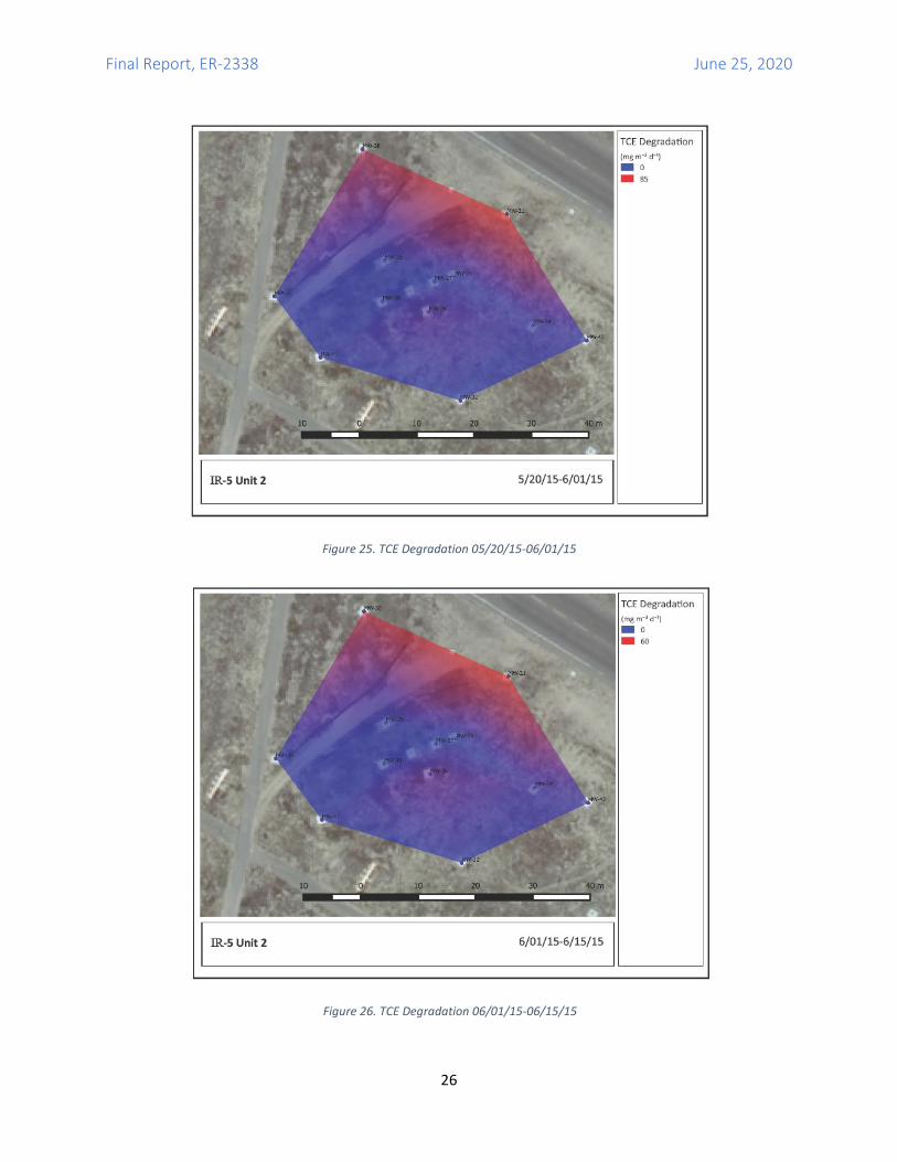
Final Report, ER-2338 June 25, 2020
26
Figure 26. TCE Degradation 06/01/15-06/15/15
Figure 25. TCE Degradation 05/20/15-06/01/15
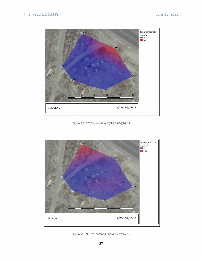
Final Report, ER-2338 June 25, 2020
27
Figure 27. TCE Degradation 06/15/15-06/28/15
Figure 28. TCE Degradation 06/28/15-07/20/15
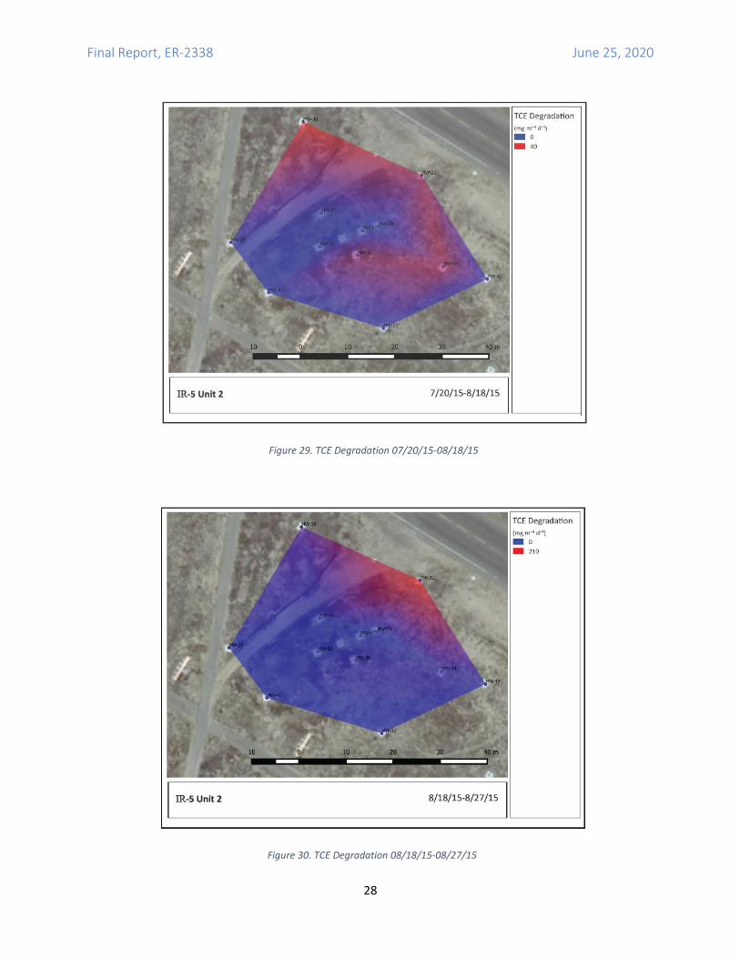
Final Report, ER-2338 June 25, 2020
28
Figure 29. TCE Degradation 07/20/15-08/18/15
Figure 30. TCE Degradation 08/18/15-08/27/15
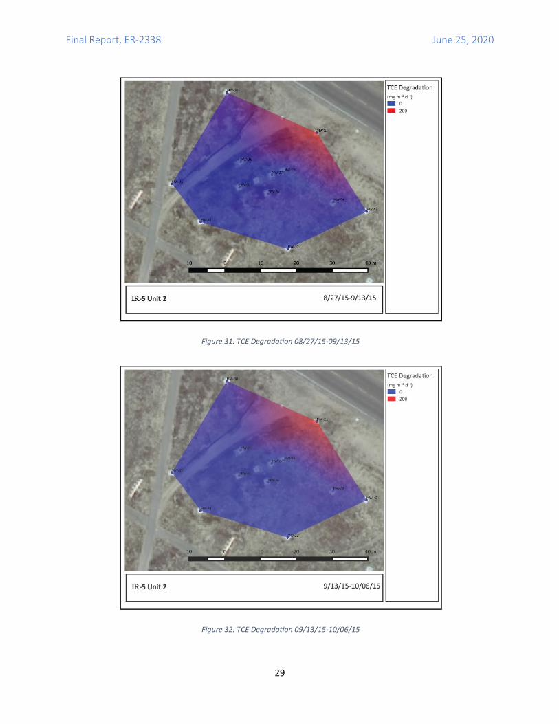
Final Report, ER-2338 June 25, 2020
29
Figure 32. TCE Degradation 09/13/15-10/06/15
Figure 31. TCE Degradation 08/27/15-09/13/15
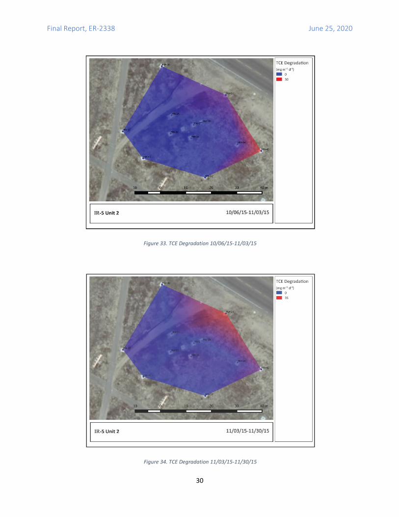
Final Report, ER-2338 June 25, 2020
30
Figure 33. TCE Degradation 10/06/15-11/03/15
Figure 34. TCE Degradation 11/03/15-11/30/15
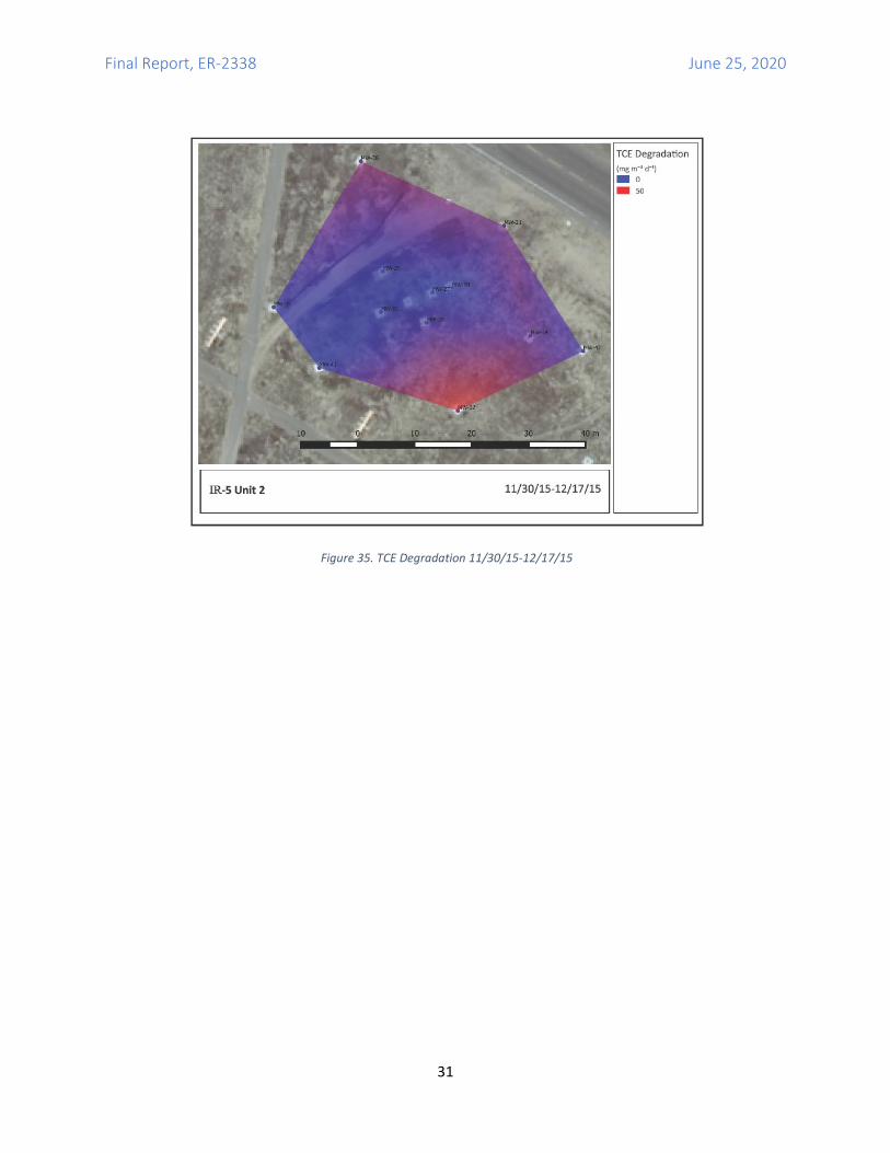
Final Report, ER-2338 June 25, 2020
31
Figure 35. TCE Degradation 11/30/15-12/17/15
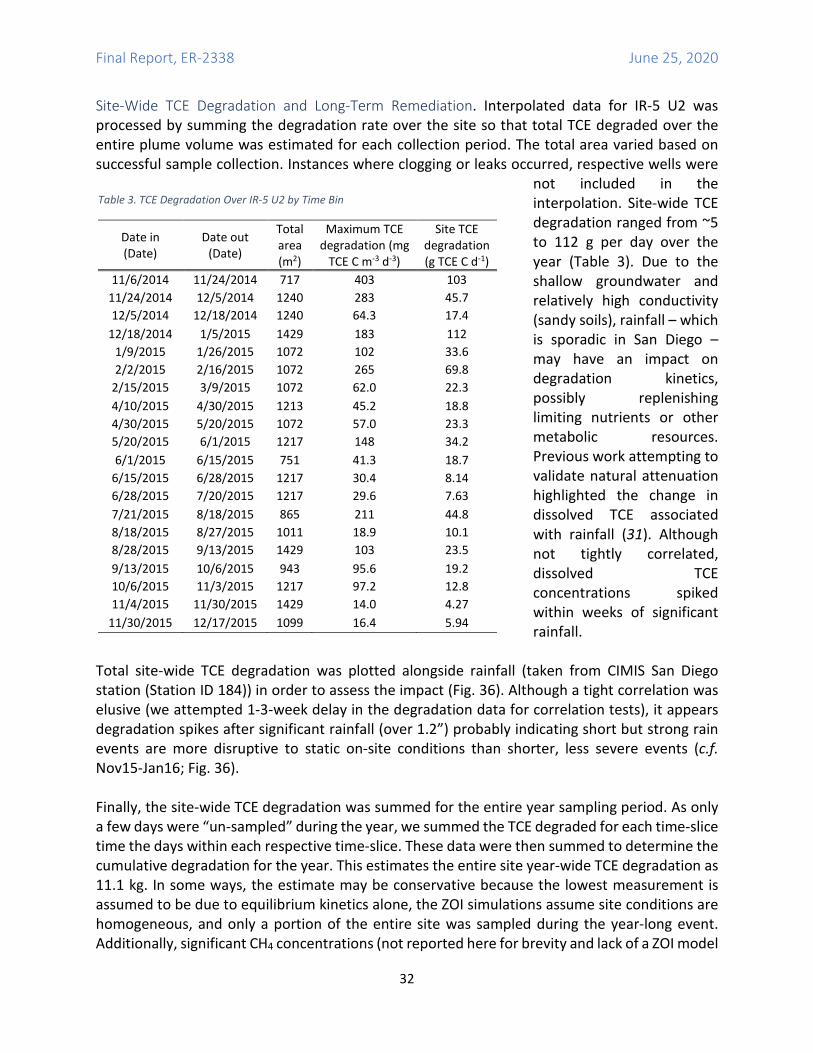
Final Report, ER-2338 June 25, 2020
32
Site-Wide TCE Degradation and Long-Term Remediation. Interpolated data for IR-5 U2 was processed by summing the degradation rate over the site so that total TCE degraded over the entire plume volume was estimated for each collection period. The total area varied based on successful sample collection. Instances where clogging or leaks occurred, respective wells were
not included in the interpolation. Site-wide TCE degradation ranged from ~5 to 112 g per day over the year (Table 3). Due to the shallow groundwater and relatively high conductivity (sandy soils), rainfall – which is sporadic in San Diego – may have an impact on degradation kinetics, possibly replenishing limiting nutrients or other metabolic resources. Previous work attempting to validate natural attenuation highlighted the change in dissolved TCE associated with rainfall (31). Although not tightly correlated, dissolved TCE concentrations spiked within weeks of significant rainfall.
Total site-wide TCE degradation was plotted alongside rainfall (taken from CIMIS San Diego station (Station ID 184)) in order to assess the impact (Fig. 36). Although a tight correlation was elusive (we attempted 1-3-week delay in the degradation data for correlation tests), it appears degradation spikes after significant rainfall (over 1.2”) probably indicating short but strong rain events are more disruptive to static on-site conditions than shorter, less severe events (c.f. Nov15-Jan16; Fig. 36). Finally, the site-wide TCE degradation was summed for the entire year sampling period. As only a few days were “un-sampled” during the year, we summed the TCE degraded for each time-slice time the days within each respective time-slice. These data were then summed to determine the cumulative degradation for the year. This estimates the entire site year-wide TCE degradation as 11.1 kg. In some ways, the estimate may be conservative because the lowest measurement is assumed to be due to equilibrium kinetics alone, the ZOI simulations assume site conditions are homogeneous, and only a portion of the entire site was sampled during the year-long event. Additionally, significant CH4 concentrations (not reported here for brevity and lack of a ZOI model
Table 3. TCE Degradation Over IR-5 U2 by Time Bin
Date in (Date)
Date out (Date)
Total area (m2)
Maximum TCE degradation (mg
TCE C m-3 d-3)
Site TCE degradation (g TCE C d-1)
11/6/2014 11/24/2014 717 403 103 11/24/2014 12/5/2014 1240 283 45.7 12/5/2014 12/18/2014 1240 64.3 17.4
12/18/2014 1/5/2015 1429 183 112 1/9/2015 1/26/2015 1072 102 33.6 2/2/2015 2/16/2015 1072 265 69.8
2/15/2015 3/9/2015 1072 62.0 22.3 4/10/2015 4/30/2015 1213 45.2 18.8 4/30/2015 5/20/2015 1072 57.0 23.3 5/20/2015 6/1/2015 1217 148 34.2 6/1/2015 6/15/2015 751 41.3 18.7
6/15/2015 6/28/2015 1217 30.4 8.14 6/28/2015 7/20/2015 1217 29.6 7.63 7/21/2015 8/18/2015 865 211 44.8 8/18/2015 8/27/2015 1011 18.9 10.1 8/28/2015 9/13/2015 1429 103 23.5 9/13/2015 10/6/2015 943 95.6 19.2 10/6/2015 11/3/2015 1217 97.2 12.8 11/4/2015 11/30/2015 1429 14.0 4.27
11/30/2015 12/17/2015 1099 16.4 5.94
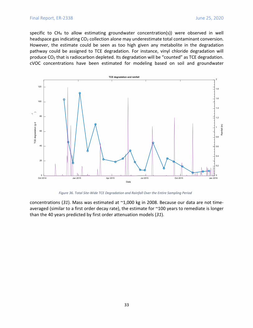
Final Report, ER-2338 June 25, 2020
33
specific to CH4 to allow estimating groundwater concentration(s)) were observed in well headspace gas indicating CO2 collection alone may underestimate total contaminant conversion. However, the estimate could be seen as too high given any metabolite in the degradation pathway could be assigned to TCE degradation. For instance, vinyl chloride degradation will produce CO2 that is radiocarbon depleted. Its degradation will be “counted” as TCE degradation. cVOC concentrations have been estimated for modeling based on soil and groundwater
concentrations (31). Mass was estimated at ~1,000 kg in 2008. Because our data are not time-averaged (similar to a first order decay rate), the estimate for ~100 years to remediate is longer than the 40 years predicted by first order attenuation models (31).
Oct 2014 Jan 2015 Apr 2015 Jul 2015 Oct 2015 Jan 2016
Date
0
20
40
60
80
100
120
TCE
degr
adat
ion
(g d
-1)
TCE degradation and rainfall
0
0.2
0.4
0.6
0.8
1
1.2
1.4
1.6
1.8
2
Rai
nfal
l (in
)
Figure 36. Total Site-Wide TCE Degradation and Rainfall Over the Entire Sampling Period
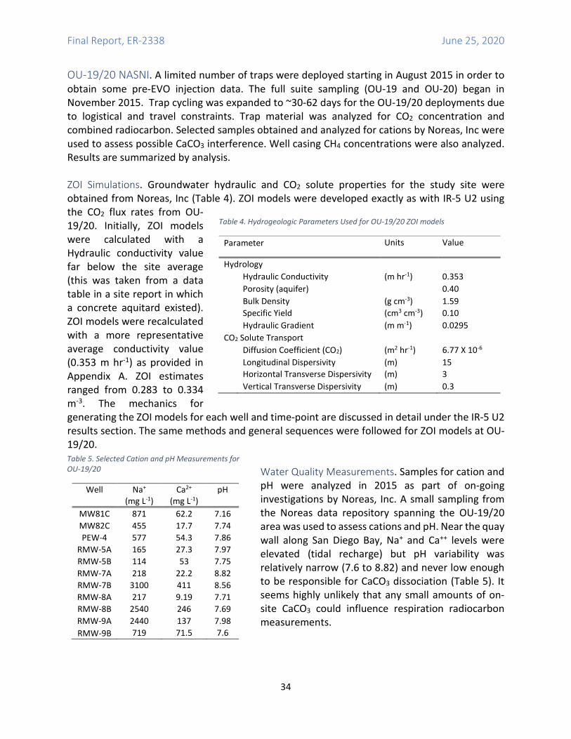
Final Report, ER-2338 June 25, 2020
34
OU-19/20 NASNI. A limited number of traps were deployed starting in August 2015 in order to obtain some pre-EVO injection data. The full suite sampling (OU-19 and OU-20) began in November 2015. Trap cycling was expanded to ~30-62 days for the OU-19/20 deployments due to logistical and travel constraints. Trap material was analyzed for CO2 concentration and combined radiocarbon. Selected samples obtained and analyzed for cations by Noreas, Inc were used to assess possible CaCO3 interference. Well casing CH4 concentrations were also analyzed. Results are summarized by analysis. ZOI Simulations. Groundwater hydraulic and CO2 solute properties for the study site were obtained from Noreas, Inc (Table 4). ZOI models were developed exactly as with IR-5 U2 using the CO2 flux rates from OU-19/20. Initially, ZOI models were calculated with a Hydraulic conductivity value far below the site average (this was taken from a data table in a site report in which a concrete aquitard existed). ZOI models were recalculated with a more representative average conductivity value (0.353 m hr-1) as provided in Appendix A. ZOI estimates ranged from 0.283 to 0.334 m-3. The mechanics for generating the ZOI models for each well and time-point are discussed in detail under the IR-5 U2 results section. The same methods and general sequences were followed for ZOI models at OU-19/20.
Water Quality Measurements. Samples for cation and pH were analyzed in 2015 as part of on-going investigations by Noreas, Inc. A small sampling from the Noreas data repository spanning the OU-19/20 area was used to assess cations and pH. Near the quay wall along San Diego Bay, Na+ and Ca++ levels were elevated (tidal recharge) but pH variability was relatively narrow (7.6 to 8.82) and never low enough to be responsible for CaCO3 dissociation (Table 5). It seems highly unlikely that any small amounts of on-site CaCO3 could influence respiration radiocarbon measurements.
Table 5. Selected Cation and pH Measurements for OU-19/20
Well
Na+ (mg L-1)
Ca2+ (mg L-1)
pH
MW81C 871 62.2 7.16 MW82C 455 17.7 7.74 PEW-4 577 54.3 7.86
RMW-5A 165 27.3 7.97 RMW-5B 114 53 7.75 RMW-7A 218 22.2 8.82 RMW-7B 3100 411 8.56 RMW-8A 217 9.19 7.71 RMW-8B 2540 246 7.69 RMW-9A 2440 137 7.98 RMW-9B 719 71.5 7.6
Table 4. Hydrogeologic Parameters Used for OU-19/20 ZOI models
Parameter Units Value
Hydrology Hydraulic Conductivity (m hr-1) 0.353 Porosity (aquifer) 0.40 Bulk Density (g cm-3) 1.59 Specific Yield (cm3 cm-3) 0.10 Hydraulic Gradient (m m-1) 0.0295 CO2 Solute Transport Diffusion Coefficient (CO2) (m2 hr-1) 6.77 X 10⁻⁶ Longitudinal Dispersivity (m) 15 Horizontal Transverse Dispersivity (m) 3 Vertical Transverse Dispersivity (m) 0.3
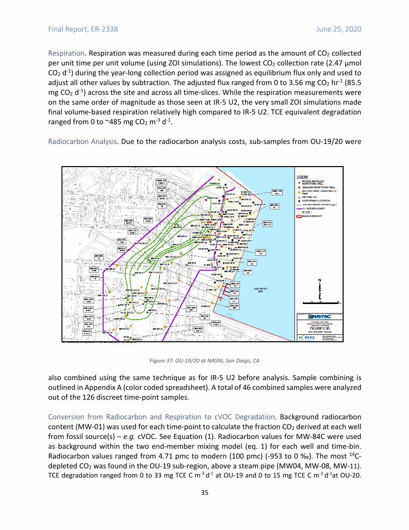
Final Report, ER-2338 June 25, 2020
35
Respiration. Respiration was measured during each time period as the amount of CO2 collected per unit time per unit volume (using ZOI simulations). The lowest CO2 collection rate (2.47 µmol CO2 d-1) during the year-long collection period was assigned as equilibrium flux only and used to adjust all other values by subtraction. The adjusted flux ranged from 0 to 3.56 mg CO2 hr-1 (85.5 mg CO2 d-1) across the site and across all time-slices. While the respiration measurements were on the same order of magnitude as those seen at IR-5 U2, the very small ZOI simulations made final volume-based respiration relatively high compared to IR-5 U2. TCE equivalent degradation ranged from 0 to ~485 mg CO2 m-3 d-1. Radiocarbon Analysis. Due to the radiocarbon analysis costs, sub-samples from OU-19/20 were
also combined using the same technique as for IR-5 U2 before analysis. Sample combining is outlined in Appendix A (color coded spreadsheet). A total of 46 combined samples were analyzed out of the 126 discreet time-point samples. Conversion from Radiocarbon and Respiration to cVOC Degradation. Background radiocarbon content (MW-01) was used for each time-point to calculate the fraction CO2 derived at each well from fossil source(s) – e.g. cVOC. See Equation (1). Radiocarbon values for MW-84C were used as background within the two end-member mixing model (eq. 1) for each well and time-bin. Radiocarbon values ranged from 4.71 pmc to modern (100 pmc) (-953 to 0 ‰). The most 14C-depleted CO2 was found in the OU-19 sub-region, above a steam pipe (MW04, MW-08, MW-11). TCE degradation ranged from 0 to 33 mg TCE C m-3 d-1 at OU-19 and 0 to 15 mg TCE C m-3 d-1at OU-20.
Figure 37. OU-19/20 at NASNI, San Diego, CA
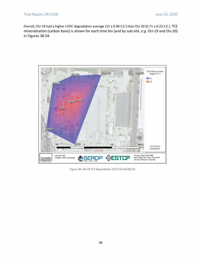
Final Report, ER-2338 June 25, 2020
36
Overall, OU-19 had a higher cVOC degradation average (15 ± 0.96 S.E.) than OU-20 (0.71 ± 0.25 S.E.). TCE mineralization (carbon basis) is shown for each time bin (and by sub-site, e.g. OU-19 and OU-20) in Figures 38-54.
Figure 38. OU-19 TCE Degradation 12/17/15-02/02/16
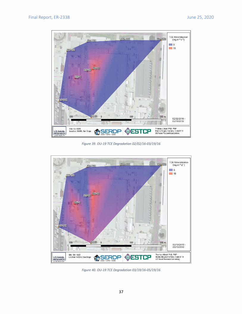
Final Report, ER-2338 June 25, 2020
37
Figure 40. OU-19 TCE Degradation 03/19/16-05/19/16
Figure 39. OU-19 TCE Degradation 02/02/16-03/19/16
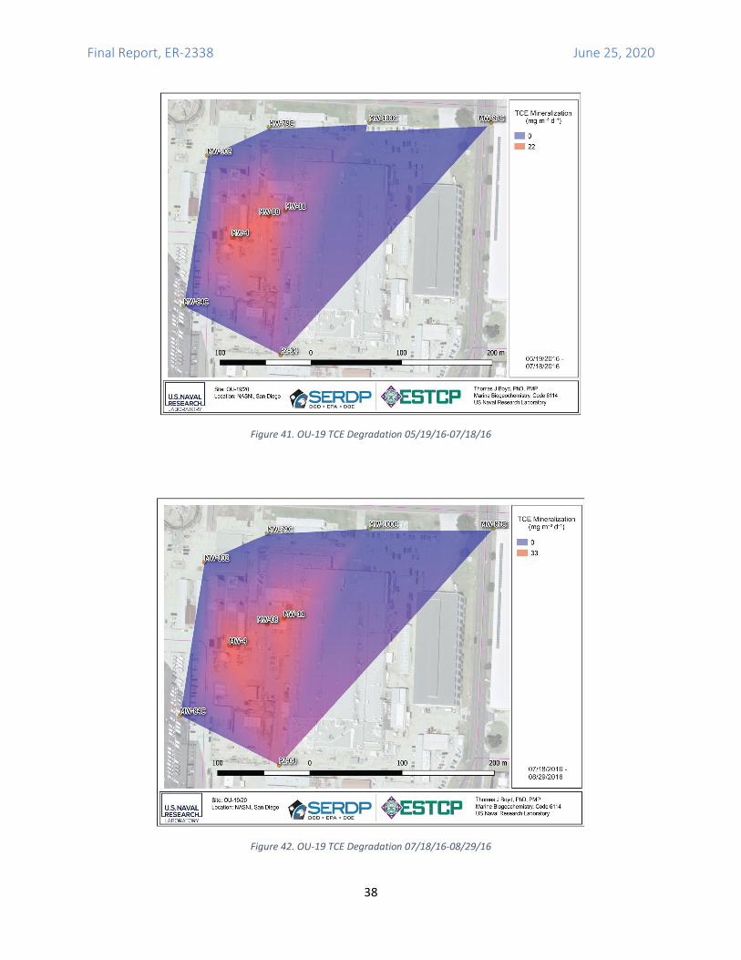
Final Report, ER-2338 June 25, 2020
38
Figure 41. OU-19 TCE Degradation 05/19/16-07/18/16
Figure 42. OU-19 TCE Degradation 07/18/16-08/29/16
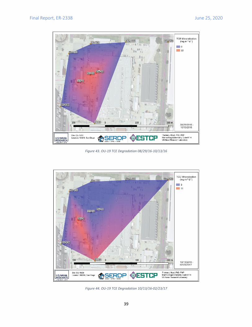
Final Report, ER-2338 June 25, 2020
39
Figure 43. OU-19 TCE Degradation 08/29/16-10/13/16
Figure 44. OU-19 TCE Degradation 10/13/16-02/23/17
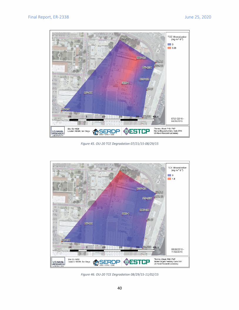
Final Report, ER-2338 June 25, 2020
40
Figure 45. OU-20 TCE Degradation 07/21/15-08/29/15
Figure 46. OU-20 TCE Degradation 08/29/15-11/02/15
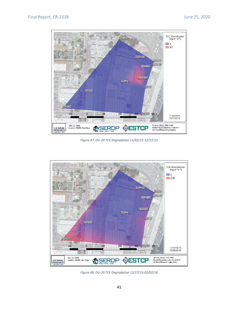
Final Report, ER-2338 June 25, 2020
41
Figure 47. OU-20 TCE Degradation 11/02/15-12/17/15
Figure 48. OU-20 TCE Degradation 12/17/15-02/02/16
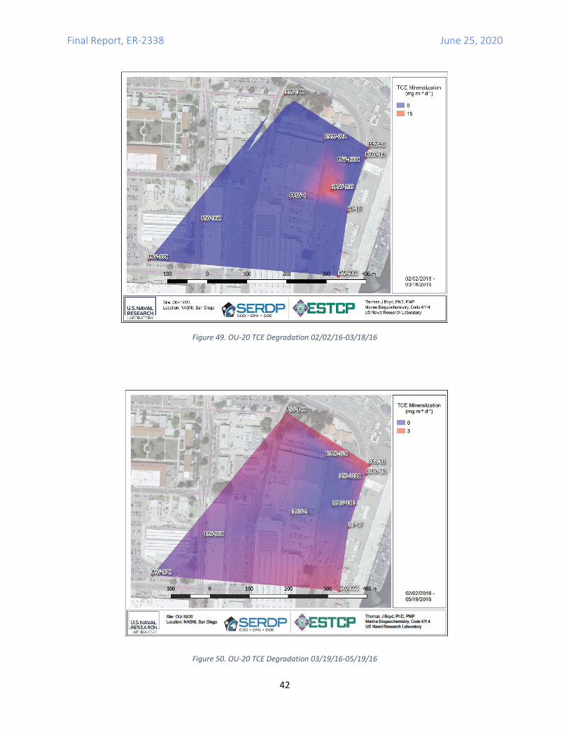
Final Report, ER-2338 June 25, 2020
42
Figure 49. OU-20 TCE Degradation 02/02/16-03/18/16
Figure 50. OU-20 TCE Degradation 03/19/16-05/19/16
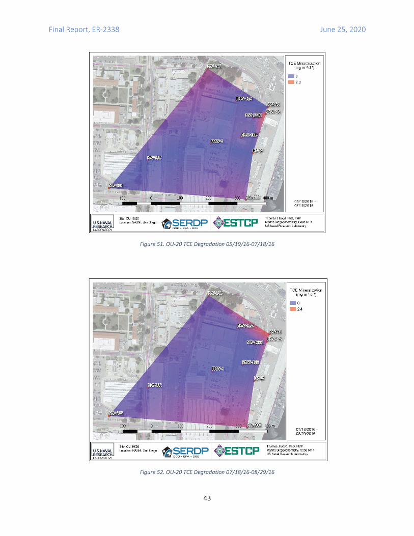
Final Report, ER-2338 June 25, 2020
43
Figure 51. OU-20 TCE Degradation 05/19/16-07/18/16
Figure 52. OU-20 TCE Degradation 07/18/16-08/29/16
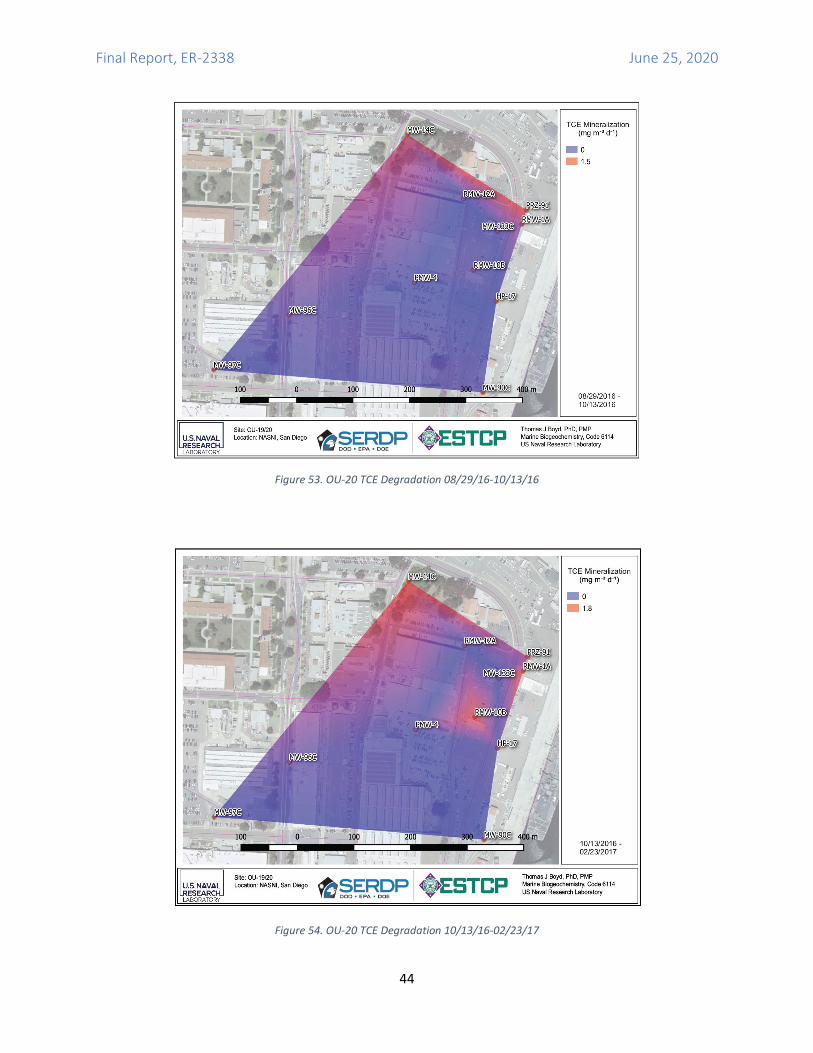
Final Report, ER-2338 June 25, 2020
44
Figure 53. OU-20 TCE Degradation 08/29/16-10/13/16
Figure 54. OU-20 TCE Degradation 10/13/16-02/23/17
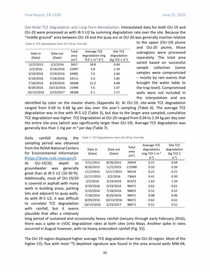
Final Report, ER-2338 June 25, 2020
45
Site-Wide TCE Degradation and Long-Term Remediation. Interpolated data for both OU-19 and OU-20 were processed as with IR-5 U2 by summing degradation rate over the site. Because the “middle ground” area between OU-19 and the quay are at OU-20 was generally inactive relative
to the upper (OU-19) plume and OU-20 plume, those subregions were processed separately. The total area varied based on successful sample collection (some samples were compromised – mostly by rain events that brought the water table to the trap level). Compromised wells were not included in the interpolation and are
identified by color on the master sheets (Appendix A). At OU-19, site-wide TCE degradation ranged from 0.69 to 4.68 kg per day over the year’s sampling (Table 6). The average TCE degradation was in-line with IR-5 U2 (Table 3), but due to the larger area sampled, cumulative TCE degradation was higher. TCE Degradation at OU-20 ranged from 0.04 to 1.34 kg per day over the entire site area (which was significantly larger than OU-19). Average TCE degradation was generally less than 1 mg per m-3 per day (Table 7). Daily rainfall during the sampling period was obtained from the NOAA National Centers for Environmental Information (https://www.ncdc.noaa.gov/). At OU-19/20, depth to groundwater was generally great than at IR-5 U2 (10-30 ft). Additionally, most of OU-19/20 is covered in asphalt with many wells in building areas, parking lots and adjacent to quay walls. As with IR-5 U2, it was difficult to correlate TCE degradation with rainfall, but it seems plausible that after a relatively long period of sustained and occasionally heavy rainfall (January through early February 2016), there was a spike in cVOC degradation rates at both sites (into May). Another spike in rates occurred in August however, with no heavy antecedent rainfall (Fig. 55). The OU-19 region displayed higher average TCE degradation than the OU-20 region. Most of the higher CO2 flux with most 14C-depleted signature was found in the area around wells MW-04,
Table 6. TCE degradation Over OU-19 by Time Bin
Date in (Date)
Date out (Date)
Total area (m2)
Average TCE degradation (mg
TCE C m-3 d-3)
Site TCE degradation (kg TCE C d-1)
12/2/2015 2/2/2016 3657 18.8 0.69 2/2/2016 3/19/2016 22997 5.8 1.34
3/19/2016 5/19/2016 34981 7.6 2.66 5/19/2016 7/18/2016 54111 3.4 1.85 7/18/2016 8/29/2016 38288 12.2 4.68 8/29/2016 10/13/2016 21996 7.6 1.67
10/13/2016 2/23/2017 38288 4.1 1.57
Table 7. TCE Degradation Over OU-20 by Time Bin
Date in (Date)
Date out (Date)
Total area (m2)
Average TCE degradation
(mg TCE C m-3 d-3)
Site TCE degradation
(kg TCE C d-1)
7/21/2015 8/26/2015 20434 0.21 0.04 8/26/2015 11/2/2015 115990 0.33 0.39 11/2/2015 12/17/2015 94516 0.21 0.21
12/17/2015 2/2/2016 73663 0.41 0.30 2/2/2016 3/19/2016 81972 1.63 1.34
3/19/2016 5/19/2016 98471 0.62 0.61 5/19/2016 7/18/2016 98825 0.52 0.52 7/18/2016 8/29/2016 98471 0.98 0.96 8/29/2016 10/13/2016 98471 0.62 0.61
10/13/2016 2/23/2017 98471 0.51 0.51
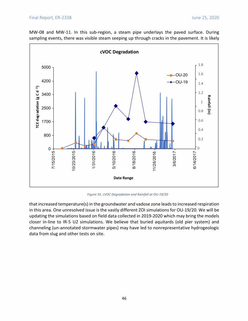
Final Report, ER-2338 June 25, 2020
46
MW-08 and MW-11. In this sub-region, a steam pipe underlays the paved surface. During sampling events, there was visible steam seeping up through cracks in the pavement. It is likely
that increased temperature(s) in the groundwater and vadose zone leads to increased respiration in this area. One unresolved issue is the vastly different ZOI simulations for OU-19/20. We will be updating the simulations based on field data collected in 2019-2020 which may bring the models closer in-line to IR-5 U2 simulations. We believe that buried aquitards (old pier system) and channeling (un-annotated stormwater pipes) may have led to nonrepresentative hydrogeologic data from slug and other tests on site.
Figure 55. cVOC Degradation and Rainfall at OU-19/20
0
800
1700
2500
3400
4200
5000
7/15
/201
5
10/2
3/20
15
1/31
/201
6
5/10
/201
6
8/18
/201
6
11/2
6/20
16
3/6/
2017
6/14
/201
7
TCE
Rainfall (in) d
egra
datio
n(g
C d
-1)
Date Range
cVOC Degradation
OU-20OU-19
0
0.2
0.4
0.6
0.8
1
1.2
1.4
1.6
1.8
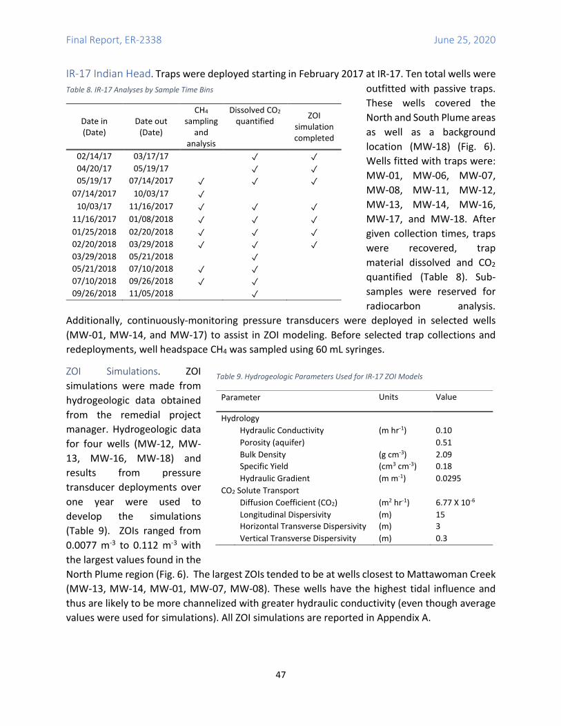
Final Report, ER-2338 June 25, 2020
47
IR-17 Indian Head. Traps were deployed starting in February 2017 at IR-17. Ten total wells were outfitted with passive traps. These wells covered the North and South Plume areas as well as a background location (MW-18) (Fig. 6). Wells fitted with traps were: MW-01, MW-06, MW-07, MW-08, MW-11, MW-12, MW-13, MW-14, MW-16, MW-17, and MW-18. After given collection times, traps were recovered, trap material dissolved and CO2 quantified (Table 8). Sub-samples were reserved for radiocarbon analysis.
Additionally, continuously-monitoring pressure transducers were deployed in selected wells (MW-01, MW-14, and MW-17) to assist in ZOI modeling. Before selected trap collections and redeployments, well headspace CH4 was sampled using 60 mL syringes.
ZOI Simulations. ZOI simulations were made from hydrogeologic data obtained from the remedial project manager. Hydrogeologic data for four wells (MW-12, MW-13, MW-16, MW-18) and results from pressure transducer deployments over one year were used to develop the simulations (Table 9). ZOIs ranged from 0.0077 m-3 to 0.112 m-3 with the largest values found in the North Plume region (Fig. 6). The largest ZOIs tended to be at wells closest to Mattawoman Creek (MW-13, MW-14, MW-01, MW-07, MW-08). These wells have the highest tidal influence and thus are likely to be more channelized with greater hydraulic conductivity (even though average values were used for simulations). All ZOI simulations are reported in Appendix A.
Table 8. IR-17 Analyses by Sample Time Bins
Date in (Date)
Date out (Date)
CH4 sampling
and analysis
Dissolved CO2 quantified ZOI
simulation completed
02/14/17 03/17/17 ✓ ✓ 04/20/17 05/19/17 ✓ ✓ 05/19/17 07/14/2017 ✓ ✓ ✓
07/14/2017 10/03/17 ✓ 10/03/17 11/16/2017 ✓ ✓ ✓
11/16/2017 01/08/2018 ✓ ✓ ✓ 01/25/2018 02/20/2018 ✓ ✓ ✓ 02/20/2018 03/29/2018 ✓ ✓ ✓ 03/29/2018 05/21/2018 ✓ 05/21/2018 07/10/2018 ✓ ✓ 07/10/2018 09/26/2018 ✓ ✓ 09/26/2018 11/05/2018 ✓
Table 9. Hydrogeologic Parameters Used for IR-17 ZOI Models
Parameter Units Value
Hydrology Hydraulic Conductivity (m hr-1) 0.10 Porosity (aquifer) 0.51 Bulk Density (g cm-3) 2.09 Specific Yield (cm3 cm-3) 0.18 Hydraulic Gradient (m m-1) 0.0295 CO2 Solute Transport Diffusion Coefficient (CO2) (m2 hr-1) 6.77 X 10⁻⁶ Longitudinal Dispersivity (m) 15 Horizontal Transverse Dispersivity (m) 3 Vertical Transverse Dispersivity (m) 0.3
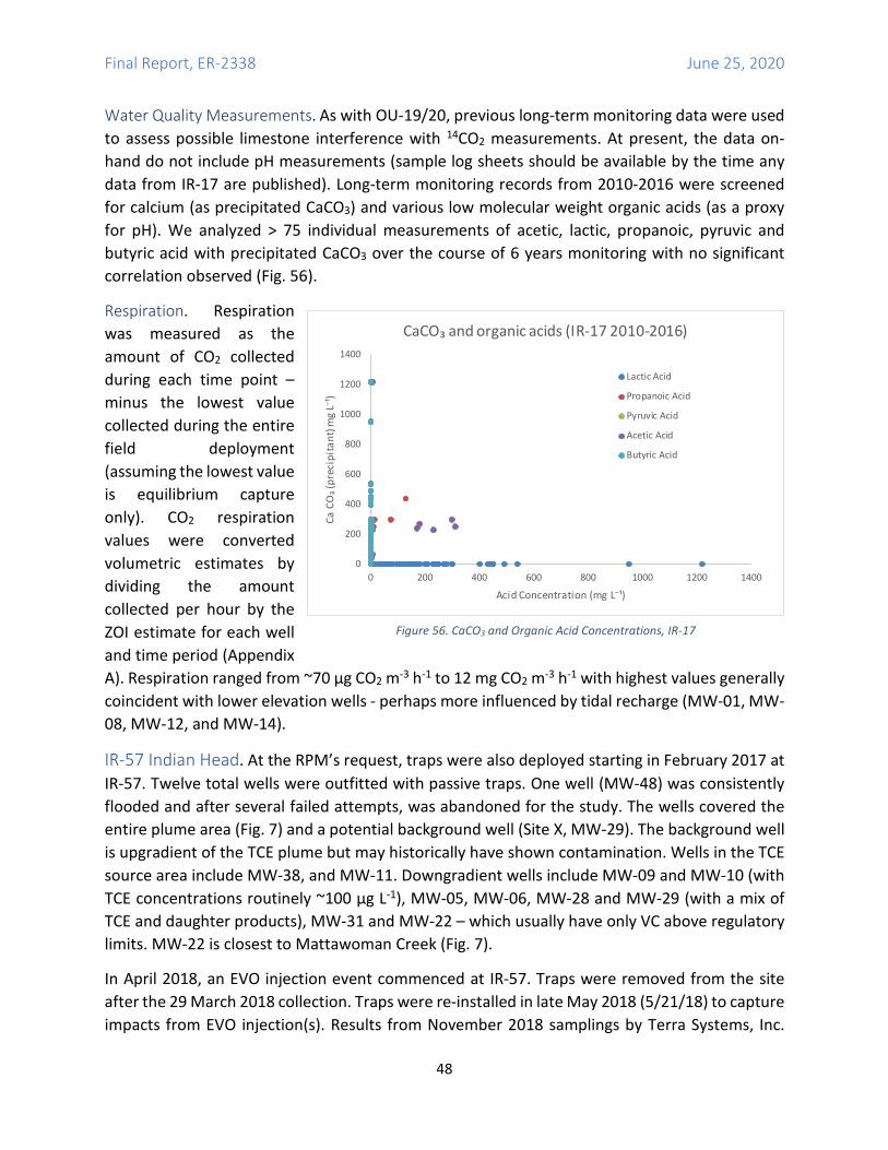
Final Report, ER-2338 June 25, 2020
48
Water Quality Measurements. As with OU-19/20, previous long-term monitoring data were used to assess possible limestone interference with 14CO2 measurements. At present, the data on-hand do not include pH measurements (sample log sheets should be available by the time any data from IR-17 are published). Long-term monitoring records from 2010-2016 were screened for calcium (as precipitated CaCO3) and various low molecular weight organic acids (as a proxy for pH). We analyzed > 75 individual measurements of acetic, lactic, propanoic, pyruvic and butyric acid with precipitated CaCO3 over the course of 6 years monitoring with no significant correlation observed (Fig. 56).
Respiration. Respiration was measured as the amount of CO2 collected during each time point – minus the lowest value collected during the entire field deployment (assuming the lowest value is equilibrium capture only). CO2 respiration values were converted volumetric estimates by dividing the amount collected per hour by the ZOI estimate for each well and time period (Appendix A). Respiration ranged from ~70 µg CO2 m-3 h-1 to 12 mg CO2 m-3 h-1 with highest values generally coincident with lower elevation wells - perhaps more influenced by tidal recharge (MW-01, MW-08, MW-12, and MW-14).
IR-57 Indian Head. At the RPM’s request, traps were also deployed starting in February 2017 at IR-57. Twelve total wells were outfitted with passive traps. One well (MW-48) was consistently flooded and after several failed attempts, was abandoned for the study. The wells covered the entire plume area (Fig. 7) and a potential background well (Site X, MW-29). The background well is upgradient of the TCE plume but may historically have shown contamination. Wells in the TCE source area include MW-38, and MW-11. Downgradient wells include MW-09 and MW-10 (with TCE concentrations routinely ~100 µg L-1), MW-05, MW-06, MW-28 and MW-29 (with a mix of TCE and daughter products), MW-31 and MW-22 – which usually have only VC above regulatory limits. MW-22 is closest to Mattawoman Creek (Fig. 7).
In April 2018, an EVO injection event commenced at IR-57. Traps were removed from the site after the 29 March 2018 collection. Traps were re-installed in late May 2018 (5/21/18) to capture impacts from EVO injection(s). Results from November 2018 samplings by Terra Systems, Inc.
0
200
400
600
800
1000
1200
1400
0 200 400 600 800 1000 1200 1400
Ca C
O₃ (
prec
ipita
nt) m
g L⁻
¹)
Acid Concentration (mg L⁻¹)
CaCO₃ and organic acids (IR-17 2010-2016)
Lactic Acid
Propanoic Acid
Pyruvic Acid
Acetic Acid
Butyric Acid
Figure 56. CaCO3 and Organic Acid Concentrations, IR-17
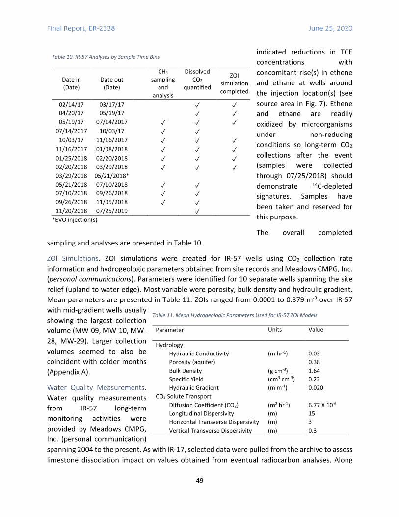
Final Report, ER-2338 June 25, 2020
49
indicated reductions in TCE concentrations with concomitant rise(s) in ethene and ethane at wells around the injection location(s) (see source area in Fig. 7). Ethene and ethane are readily oxidized by microorganisms under non-reducing conditions so long-term CO2 collections after the event (samples were collected through 07/25/2018) should demonstrate 14C-depleted signatures. Samples have been taken and reserved for this purpose.
The overall completed sampling and analyses are presented in Table 10.
ZOI Simulations. ZOI simulations were created for IR-57 wells using CO2 collection rate information and hydrogeologic parameters obtained from site records and Meadows CMPG, Inc. (personal communications). Parameters were identified for 10 separate wells spanning the site relief (upland to water edge). Most variable were porosity, bulk density and hydraulic gradient. Mean parameters are presented in Table 11. ZOIs ranged from 0.0001 to 0.379 m-3 over IR-57 with mid-gradient wells usually showing the largest collection volume (MW-09, MW-10, MW-28, MW-29). Larger collection volumes seemed to also be coincident with colder months (Appendix A).
Water Quality Measurements. Water quality measurements from IR-57 long-term monitoring activities were provided by Meadows CMPG, Inc. (personal communication) spanning 2004 to the present. As with IR-17, selected data were pulled from the archive to assess limestone dissociation impact on values obtained from eventual radiocarbon analyses. Along
Table 11. Mean Hydrogeologic Parameters Used for IR-57 ZOI Models
Parameter Units Value
Hydrology Hydraulic Conductivity (m hr-1) 0.03 Porosity (aquifer) 0.38 Bulk Density (g cm-3) 1.64 Specific Yield (cm3 cm-3) 0.22 Hydraulic Gradient (m m-1) 0.020 CO2 Solute Transport Diffusion Coefficient (CO2) (m2 hr-1) 6.77 X 10⁻⁶ Longitudinal Dispersivity (m) 15 Horizontal Transverse Dispersivity (m) 3 Vertical Transverse Dispersivity (m) 0.3
Table 10. IR-57 Analyses by Sample Time Bins
Date in (Date)
Date out (Date)
CH4 sampling
and analysis
Dissolved CO2
quantified
ZOI simulation completed
02/14/17 03/17/17 ✓ ✓ 04/20/17 05/19/17 ✓ ✓ 05/19/17 07/14/2017 ✓ ✓ ✓
07/14/2017 10/03/17 ✓ ✓ 10/03/17 11/16/2017 ✓ ✓ ✓
11/16/2017 01/08/2018 ✓ ✓ ✓ 01/25/2018 02/20/2018 ✓ ✓ ✓ 02/20/2018 03/29/2018 ✓ ✓ ✓ 03/29/2018 05/21/2018* 05/21/2018 07/10/2018 ✓ ✓ 07/10/2018 09/26/2018 ✓ ✓ 09/26/2018 11/05/2018 ✓ ✓ 11/20/2018 07/25/2019 ✓
*EVO injection(s)
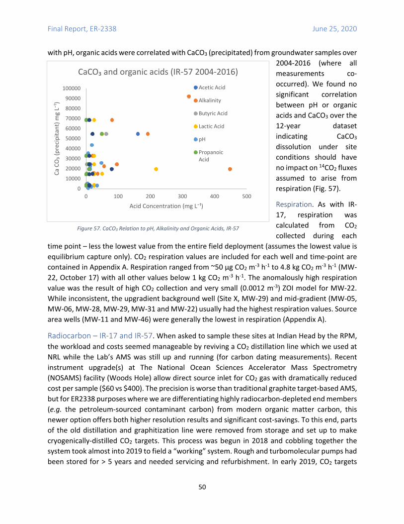
Final Report, ER-2338 June 25, 2020
50
with pH, organic acids were correlated with CaCO3 (precipitated) from groundwater samples over 2004-2016 (where all measurements co-occurred). We found no significant correlation between pH or organic acids and CaCO3 over the 12-year dataset indicating CaCO3 dissolution under site conditions should have no impact on 14CO2 fluxes assumed to arise from respiration (Fig. 57).
Respiration. As with IR-17, respiration was calculated from CO2 collected during each
time point – less the lowest value from the entire field deployment (assumes the lowest value is equilibrium capture only). CO2 respiration values are included for each well and time-point are contained in Appendix A. Respiration ranged from ~50 µg CO2 m-3 h-1 to 4.8 kg CO2 m-3 h-1 (MW-22, October 17) with all other values below 1 kg CO2 m-3 h-1. The anomalously high respiration value was the result of high CO2 collection and very small (0.0012 m-3) ZOI model for MW-22. While inconsistent, the upgradient background well (Site X, MW-29) and mid-gradient (MW-05, MW-06, MW-28, MW-29, MW-31 and MW-22) usually had the highest respiration values. Source area wells (MW-11 and MW-46) were generally the lowest in respiration (Appendix A).
Radiocarbon – IR-17 and IR-57. When asked to sample these sites at Indian Head by the RPM, the workload and costs seemed manageable by reviving a CO2 distillation line which we used at NRL while the Lab’s AMS was still up and running (for carbon dating measurements). Recent instrument upgrade(s) at The National Ocean Sciences Accelerator Mass Spectrometry (NOSAMS) facility (Woods Hole) allow direct source inlet for CO2 gas with dramatically reduced cost per sample ($60 vs $400). The precision is worse than traditional graphite target-based AMS, but for ER2338 purposes where we are differentiating highly radiocarbon-depleted end members (e.g. the petroleum-sourced contaminant carbon) from modern organic matter carbon, this newer option offers both higher resolution results and significant cost-savings. To this end, parts of the old distillation and graphitization line were removed from storage and set up to make cryogenically-distilled CO2 targets. This process was begun in 2018 and cobbling together the system took almost into 2019 to field a “working” system. Rough and turbomolecular pumps had been stored for > 5 years and needed servicing and refurbishment. In early 2019, CO2 targets
0
10000
20000
30000
40000
50000
60000
70000
80000
90000
100000
0 100 200 300 400 500
Ca C
O₃ (
prec
ipita
nt) m
g L⁻
¹)
Acid Concentration (mg L⁻¹)
CaCO₃ and organic acids (IR-57 2004-2016)Acetic Acid
Alkalinity
Butyric Acid
Lactic Acid
pH
PropanoicAcid
Figure 57. CaCO3 Relation to pH, Alkalinity and Organic Acids, IR-57
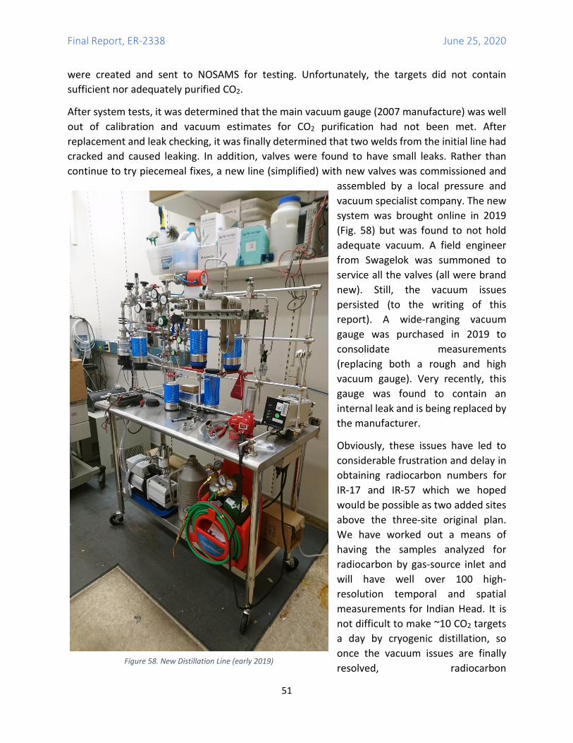
Final Report, ER-2338 June 25, 2020
51
were created and sent to NOSAMS for testing. Unfortunately, the targets did not contain sufficient nor adequately purified CO2.
After system tests, it was determined that the main vacuum gauge (2007 manufacture) was well out of calibration and vacuum estimates for CO2 purification had not been met. After replacement and leak checking, it was finally determined that two welds from the initial line had cracked and caused leaking. In addition, valves were found to have small leaks. Rather than continue to try piecemeal fixes, a new line (simplified) with new valves was commissioned and
assembled by a local pressure and vacuum specialist company. The new system was brought online in 2019 (Fig. 58) but was found to not hold adequate vacuum. A field engineer from Swagelok was summoned to service all the valves (all were brand new). Still, the vacuum issues persisted (to the writing of this report). A wide-ranging vacuum gauge was purchased in 2019 to consolidate measurements (replacing both a rough and high vacuum gauge). Very recently, this gauge was found to contain an internal leak and is being replaced by the manufacturer.
Obviously, these issues have led to considerable frustration and delay in obtaining radiocarbon numbers for IR-17 and IR-57 which we hoped would be possible as two added sites above the three-site original plan. We have worked out a means of having the samples analyzed for radiocarbon by gas-source inlet and will have well over 100 high-resolution temporal and spatial measurements for Indian Head. It is not difficult to make ~10 CO2 targets a day by cryogenic distillation, so once the vacuum issues are finally resolved, radiocarbon
Figure 58. New Distillation Line (early 2019)

Final Report, ER-2338 June 25, 2020
52
measurements should be possible within about 6 months. We have manuscript outlines for IR-17 and IR-57 and at this point are mostly awaiting the radiocarbon data so that conclusions can be drawn.

Final Report, ER-2338 June 25, 2020
53
Conclusions and Implications for Future Research / Implementation In this project, we combined time-averaged and spatial respiration and radiocarbon measurements to determine site cVOC degradation (TCE carbon equivalents) at IR-5 U2 (Naval Air Station North Island), OU-19 (NASNI), OU-20 (NASNI) and partially completed the analysis at two sites (IR-17 and IR-57) at Indian Head Naval Surface Warfare Center (MD). These measurements were combined with a zone of influence (ZOI) model to estimate the volume sampled at each well. Plume characteristics (volume) and volumetric TCE degradation values were used to determine the annual cVOC degradation occurring over the sites studied. cVOC respiration measurements are likely conservative because we assumed the lowest rate was due to equilibrium CO2 capture only which is unlikely unless there were timepoints when no actual respiration occurred. ZOIs were calculated using site-specific hydrological data and represent a refined estimate of the sampled area compared to a single groundwater sample (representing the well only at the time of sampling). The ultimate goal was to determine the contaminant to CO2 conversion rate per unit area (m-3) per unit time (d-1). With this successful effort, we completed the following: ● Assessed sites for potential complicating factors (limestone deposits) ● Measured well head-space methane which could be a contaminant repository not evaluated as such (but planned in eventual publications) ● Measured respiration rate(s) as CO2 collected over 1-3 month time periods at 5 sites ● Measured radiocarbon content for CO2 respired at three sites ● Created ZOI models for each well and time-point sampled to determine volume sampled ● Determined respiration from contaminants by calculating the fraction CO2 derived from petroleum sources ● Determined well-specific cVOC degradation based on volumetric ZOI models and contaminant respiration ● Determined site-wide cVOC degradation using interpolation between sampled wells ● Used estimated plume dimensions to calculate site-wide degradation over relevant time-scales ● Presented results to regulators (IR-5 U2) for validation. ● Published results from IR-5 U2 in peer-reviewed literature ● Published methods and validation in peer-reviewed literature ● Performed a small comparative study (outlined in ESTCP ER19-5106) using different methods for time-averaged CO2 radiocarbon collection and calculation for cross validation. At IR-5 U2, the lowest apparent cVOC utilization was coincident with regions of highest historical contamination. There was no direct correlation (r2 < 0.50) between contaminant concentrations and cVOC utilization. CO2 collected above the high historical contamination region had the most modern carbon indicating less relative contribution from cVOC than natural organic matter.
Final Report, ER-2338 June 25, 2020
54
At OU-19/20, cVOC degradation rates were highest at the OU-19 sub-region associated with steam pipes under the pavement. At the OU-20 sub-region, cVOC degradation rates were highest at the plume fringes (as with IR-5 U2). An EVO injection event did not appear to stimulate cVOC degradation based on this method. However, this event would stimulate releasing massive quantities of modern CO2 (from vegetable oil biodegradation). It is unclear if that could mask the signal from cVOC CO2 (14C-depleted). The passive CO2 trap design changed during the project due to both difficulty in maintaining mechanical systems in the field and the inability to deploy active samplers at operable units. The only advantage of active traps is the ability to capture more CO2 per unit time. Passive traps have multiple advantages; they need no logistical support (power, pumps), they are subject to vandalism or tampering (sealed within the well headspace) and can be deployed rapidly with simple tools (wrench to open well lid). Additionally, passive samplers do not need modified pumps (sealed for recirculation) so lead-in time is very short. Passive traps need to be fabricated, but materials are readily available (PVC fittings) and inexpensive. Well caps were modified for this project, but would not have to be as well headspace could be sparged with Ar (heavier than air so it fills from the bottom) and resealed without compromising the traps. An exception would be wells in which EVO is injected. At OU-20, tremendous amounts of CH4 were produced after injection. Well caps without check valves (wells other than where we deployed) routinely had well caps “blown off” by excessive gas production. This could possibly compromise traps suspended in the headspace – although positive gas flow to the top of the well would likely obviate any incoming atmospheric gas. Future goals will be to transition the technology with different means for measuring CO2 flux:
• In-well passive CO2 traps • Soil:atmosphere CO2 flux traps • Short-term groundwater incubations to determine respiration rates
These techniques performed at the same site at the same time(s) and coupled with radiocarbon analysis would allow cross-validation and give RPMs an arsenal of techniques to answer the fundamental question whether on-site processes stimulate the conversion of cVOCs to harmless degradation end projects in a time-frame that suits site management strategies. In general, radiocarbon analyses have been expensive enough to limit their routine use. As mentioned above, newer instrumentation with gas-inlet capabilities has reduced the cost almost 10-fold (given the ability to distill or otherwise purify the CO2 before analysis). Through collaboration we have sought to interface with Dr. John Mattson at Johns Hopkins Applied Physics Lab to use a gas-source MICADAS instrument. We submitted a white paper seeking funds to purchase a Carbonate Handling Device (CHS) made by the same manufacturer (IonPlus). This device is now in generation 2 (https://www.ionplus.ch/chs2) and can accommodate 64 samples. This device sparges CO2 and transfers it purified to the gas-inlet on the MICADAS AMS. The whole procedure is completely automated. Our white paper was not successful – primarily due to cost.
Final Report, ER-2338 June 25, 2020
55
This peripheral is ~$85K. Advances in AMS and peripherals are moving fast, mostly to service the pharmaceutical industry – so costs are continually going down. For perspective, today one can obtain a stable isotope (δ13C) measurement from carbonates for ~$11 (UC Davis). The instrumentation cost is ~$450K (IRMS engine plus gas bench). The MICADAS instruments are now ~$1.1M with costs for a CHS2 peripheral. As more laboratories are fitted with these AMS instruments and peripherals, costs will eventually scale accordingly making 14C analyses more routine in environmental sciences.
In addition, new techniques using cavity ring-down laser spectroscopy are seeking to bring routine 14CO2 analyses to the benchtop (42). While still in commercialization pipelines, optical 14CO2 and 14CH4 sensor systems capable of natural abundance measurements are functioning today (43-45). Depending of course on market demand, laser-based radiocarbon instruments could be fielded similar to laser-based stable isotope instruments which have many advantages over traditional stable isotope mass spectrometers – namely cost (about 1/5 the amount), low maintenance (no vacuum components) and size (systems are similar in size to a computer CPU). Laser-based stable isotope measurements are on the order of $10-15 per sample. While there’s no guarantee that radiocarbon instruments will be fielded soon and that market demand will ensure many instruments are purchased and brought on-line, the utility inherent in radiocarbon analyses should ensure rapid adoption by multiple scientific communities. One final issue addressed in the Board comments is this technique’s validity given some comprises made in execution – primarily due to financial constraints. It is true that radiocarbon measurements without any of the newer instrumentation and AMS techniques was too expensive to employ in every sample. During the field deployments, we generated over 550 CO2 respiration samples, which at full analytical resolution would have cost over $200,000 to analyze by traditional AMS. Because this was a demonstration-type project, we were ambitious in sample collection (relative to a cost-based contractor). It should also be noted that our project was capped at $150K per year – instead of the $300K+ per year in the original request to accommodate more radiocarbon analyses. From our $150K per year there were two sub-contracts and radiocarbon analyses – plus in-house labor rate (with overhead) at NRL and travel expenses. It was simply not financially possible to analyze every sample as we had intended. With this in mind, and the ever-decreasing cost of analysis (from over $500 to $390 for full graphite target analysis to $57 for gas-source analysis which was commercially unavailable when this project started), analyses will become far more straightforward and are already far less expensive.
Final Report, ER-2338 June 25, 2020
56
Literature Cited 1. National Research Council, In situ bioremediation: When does it work? (National Academy of
Sciences, Washington, DC, 1993), pp. 1-207. 2. K. M. Vangelas, "Summary Document of Workshops for Hanford, Oak Ridge and Savannah River
Site as part of the Monitored Natural Attenuation and Enhanced Passive Remediation for Chlorinated Solvents - DOE Alternative Project for Technology Acceleration," (U.S. Department of Energy, Westinghouse Savannah River Company, Aiken, SC, 2003).
3. T. H. Wiedemeier et al., "Technical Protocol for Evaluating Natural Attenuation of Chlorinated Solvents in Ground Water," (USEPA Office of Research and Development, Washington, DC, 1998).
4. J. Šimůnek, D. L. Suarez, M. Sejna, "The UNSATCHEM Software Package for Simulating One-Dimensional Variably Saturated Water Flow, Heat Transport, Carbon Dioxide Production and Transport, and Solute Transport with Major Ion Equilibrium and Kinetic Chemistry, Version 2.0," (USDA-ARS U.S. Salinity Laboratory, Riverside, CA, 1996).
5. A. Leeson, H. F. Stroo, "SERDP and ESTCP workshop on investment strategies to optimize research and demonstration impacts in support of DoD restoration goals," (SERDP/ESTCP, Arlington, VA, 2011).
6. SERDP/ESTCP, "SERDP/ESTCP Expert Panel Workshop on Research and Development Needs for Cleanup of Chlorinated Solvent Sites," (2002).
7. J. V. Weiss, I. M. Cozzarelli, Biodegradation in contaminated aquifers: Incorporating microbial/molecular methods. Ground water 46, 305-322 (2008).
8. W. A. Illman, P. J. Alvarez, Performance assessment of bioremediation and natural attenuation. Critical Reviews in Environmental Science and Technology 39, 209-270 (2009).
9. P. Bombach, H. H. Richnow, M. Kästner, A. Fischer, Current approaches for the assessment of in situ biodegradation. Applied Microbiology and Biotechnology 86, 839-852 (2010).
10. H. B. Kerfoot, C. L. Mayer, P. B. Durgin, J. J. D'Lugosz, Measurement of Carbon Dioxide in Soil Gases for Indication of Subsurface Hydrocarbon Contamination. Ground Water Monitoring & Remediation 8, 67-71 (1988).
11. K. H. Suchomel, D. K. Kreamer, A. Long, Production and transport of carbon-dioxide in a contaminated vadose zone - a stable and radioactive carbon isotope study. Environmental Science and Technology 24, 1824-1831 (1990).
12. C. M. Aelion, C. M. Swindoll, F. K. Pfaender, Adaptation to and Biodegradation of Xenobiotic Compounds by Microbial Communities from a Pristine Aquifer. Applied and Environmental Microbiology 53, 2212-2217 (1987).
13. B. C. Kirtland, C. M. Aelion, P. A. Stone, D. Hunkeler, Isotopic and Geochemical Assessment of in Situ Biodegradation of Chlorinated Hydrocarbons. Environmental Science and Technology 37, 4205-4212 (2003).
14. B. C. Kirtland, C. M. Aelion, P. A. Stone, Assessing in situ mineralization of recalcitrant organic compounds in vadose zone sediments using δ13C and ∆14C measurements. Journal of Contaminant Hydrology 76, 1-18 (2005).
15. R. B. Coffin et al., Radiocarbon and Stable Carbon Isotope Analysis to Confirm Petroleum Natural Attenuation in the Vadose Zone. Environmental Forensics 9, 75-84 (2008).
16. T. J. Boyd, M. T. Montgomery, R. H. Cuenca, Y. Hagimoto, Measuring Carbon-based Contaminant Mineralization Using Combined CO2 Flux and Radiocarbon Analyses. Journal of Visualized Experiments, e53233 (2016).
Final Report, ER-2338 June 25, 2020
57
17. T. J. Boyd, M. T. Montgomery, R. H. Cuenca, Y. Hagimoto, Combined radiocarbon and CO2 flux measurements used to determine in situ chlorinated solvent mineralization rate. Environmental Science: Processes & Impacts 17, 683 - 692 (2015).
18. T. J. Boyd, M. J. Pound, R. H. Cuenca, Y. Hagimoto, M. T. Montgomery, "Radiocarbon Allows Direct Determination of Fuel and Industrial Chemical Degradation at ER Sites," ER News (US Naval Facilities, Port Hueneme, CA, 2014).
19. T. J. Boyd, M. J. Pound, D. Lohr, R. B. Coffin, Radiocarbon-depleted CO2 evidence for fuel biodegradation at the Naval Air Station North Island (USA) fuel farm site. Environmental Science: Processes & Impacts 15, 912-918 (2013).
20. G. C. Bugna, J. P. Chanton, T. B. Stauffer, W. G. Macintyre, E. L. Libelo, Partitioning microbial respiration between jet fuel and native organic matter in an organic-rich long time-contaminated aquifer. Chemosphere 60, 177-187 (2005).
21. T. J. Boyd, J. Gryzenia, D. Ramquist, G. M. Wyatt, "Short-term respiration measurements coupled with CO2 radiocarbon analysis provide fuel degradation rates at an underground fuel strorage tank leak site," (US Naval Research Laboratory, Washington, DC, 2018).
22. K. McCoy, J. A. Zimbron, T. Sale, M. Lyverse, Measurement of Natural Losses of LNAPL Using CO2 Traps. Groundwater 53, 658-667 (2015).
23. N. J. Sihota, K. Ulrich Mayer, Characterizing vadose zone hydrocarbon biodegradation using carbon dioxide effluxes, isotopes, and reactive transport modeling. Vadose Zone Journal 11, (2012).
24. E. Warren, N. J. Sihota, F. D. Hostettler, B. A. Bekins, Comparison of surficial CO2 efflux to other measures of subsurface crude oil degradation. Journal of Contaminant Hydrology 164, 275-284 (2014).
25. S. M. Carroll, A. D. Peacock, J. Zimbron, K. N. Alepidis, J. A. Clock, Demonstrating Contaminant Degradation at an MGP Site With Metabolic Gas Flux and Radio Carbon Dating. Remediation Journal 27, 51-64 (2017).
26. C. M. Aelion, B. C. Kirtland, P. A. Stone, Radiocarbon assessment of aerobic petroleum bioremediation in the vadose zone and groundwater at an AS/SVE site. Environmental Science and Technology 31, 3363-3370 (1997).
27. U. EPA, "BIOCHLOR Natural attenuation decision support system, User's Manual," (US EPA, Washington, DC, 2000).
28. R. U. Meckenstock, C. Griebler, B. Morasch, H. H. Richnow, Stable isotope fractionation analysis as a tool to monitor biodegradation in contaminated acquifers. Journal of Contaminant Hydrology 75, 215-255 (2004).
29. C. Vogt, C. Dorer, F. Musat, H.-H. Richnow, Multi-element isotope fractionation concepts to characterize the biodegradation of hydrocarbons — from enzymes to the environment. Current Opinion in Biotechnology 41, 90-98 (2016).
30. API, "Quantification of Vapor Phase-related Natural Source Zone Depletion Processes," (American Petroleum Institute (API), 2017).
31. S. I. Inc., "Draft Feasibility Study, Installation Restoration Site 5, Unit 2, Naval Air Station North Island, San Diego, California," (Shaw Infrastructure, Inc, Concord, CA, 2013).
32. V. Hosangadi, "Draft Appendix B Site Conceptual Model Technical Memorandum Operable Units 19/20," (Noreas, Inc, San Diego, CA, 2013).
33. M. Stuiver, H. A. Polach, Discussion: Reporting of 14C Data. Radiocarbon 19, 355-363 (1977). 34. K. M. Johnson, J. M. Sieburth, P. J. l. B. Williams, L. Brändström, Coulometric total carbon dioxide
analysis for marine studies: Automation and Calibration. Mar.Chem. 21, 117-133 (1987). 35. A. G. Dickson, Standards for ocean measurements. Oceanography 23, 34-47 (2010).
Final Report, ER-2338 June 25, 2020
58
36. C. Zheng, P. P. Wang, "MT3DMS: A modular three-dimensional multispecies transport model for simulation of advection, dispersion, and chemical reactions of contaminants in groundwater systems; documentation and user's guide," (DTIC Document, 1999).
37. A. W. Harbaugh, MODFLOW-2005, the US Geological Survey modular ground-water model: The ground-water flow process. (US Department of the Interior, US Geological Survey, 2005).
38. H. Prommer, D. A. Barry, C. Zheng, MODFLOW/MT3DMS-based reactive multicomponent transport modeling. Ground Water 41, 247-257 (2003).
39. R. B. Winston, in Ground Water - Book 6. (U.S. Geological Survey, Reston, VA, 2009), vol. Techniques and Methods 6-A29, chap. 29.
40. Accord Engineering Inc., " Semi-Annual Post-Closure Maintenance Report for Calendar Year 2011 Installation Restoration (IR) Program Site 2 (Old Spanish Bight Landfill), Site 4 (Public Works Salvage Yard), and Site 5, Unit 1 (Golf Course Landfill)," (San Diego, CA, 2011).
41. Geosyntec Consultants, "Annual Progress Report October 2010 to December 2011, Operable Unit 24," (Columbia, MD, 2012).
42. D. E. Murnick, Laser-based radiocarbon detection in the laboratory: How soon? Journal of Labelled Compounds and Radiopharmaceuticals 62, 768-775 (2019).
43. I. Galli et al., in Optics InfoBase Conference Papers. (2017), vol. Part F82-CLEO_Europe 2017. 44. I. Galli et al., in 2016 Conference on Lasers and Electro-Optics, CLEO 2016. (2016). 45. S. Larnimaa et al., High-resolution analysis of the ν3 band of radiocarbon methane 14CH4.
Chemical Physics Letters 750, (2020).
Final Report, ER-2338 June 25, 2020
59
Appendix A. Supporting Data Compiled data files for IR-5 U2, OU-19/20, IR-17, and IR-57
IR-5 U2 compiled data.xlsx
IR-5 U2 interpolation.xlsx
OU-19-20 interpolation.xlsx
IR-17 - IR-57 compiled data.xlsx
Clickable link to a Tier II SAP template amenable to new sites (with regulatory approval)
Final Report, ER-2338 June 25, 2020
60
Appendix B. List of Scientific / Technical Publications Boyd, T. J., M. J. Pound, D. Lohr and R. B. Coffin (2013). "Radiocarbon-depleted CO2 evidence for fuel biodegradation at the Naval Air Station North Island (USA) fuel farm site." Environmental Science: Processes & Impacts 15(5): 912-918. Boyd, T. J., M. T. Montgomery, R. H. Cuenca and Y. Hagimoto (2014). CO2 Radiocarbon Analysis to Quantify Organic Contaminant Degradation, MNA, and Engineered Remediation Approaches, United States Naval Research Laboratory: 59. Boyd, T. J., M. J. Pound, R. H. Cuenca, Y. Hagimoto and M. T. Montgomery (2014). Radiocarbon Allows Direct Determination of Fuel and Industrial Chemical Degradation at ER Sites. ER News. A. W. Ortiz. Port Hueneme, CA, US Naval Facilities. 14: 13-14. Boyd, T. J., M. T. Montgomery, R. H. Cuenca and Y. Hagimoto (2015). "Combined radiocarbon and CO2 flux measurements used to determine in situ chlorinated solvent mineralization rate." Environmental Science: Processes & Impacts 17(3): 683 - 692. Boyd, T. J., M. T. Montgomery, R. H. Cuenca and Y. Hagimoto (2016). "Measuring Carbon-based Contaminant Mineralization Using Combined CO2 Flux and Radiocarbon Analyses." Journal of Visualized Experiments(116): e53233. Boyd, T. J., J. Gryzenia, D. Ramquist and G. M. Wyatt (2018). Short-term respiration measurements coupled with CO2 radiocarbon analysis provide fuel degradataion rates at an underground fuel strorage tank leak site. Washington, DC, US Naval Research Laboratory. Boyd, T. J., J. A. Zimbron, R. H. Cuenca, Y. Hagimoto, C. J. Newell, J. T. Wilson and K. J. Johnson "Evaluating CO2 radiocarbon flux measurement techniques for assessing organic contaminant remediation in groundwater and vadose horizons " In Preparation.