Forecasting Foreign

Exchange Rates A comparison between forecasting horizons and

Bayesian vs. Frequentist approaches

Max Nyström Winsa

June 12, 2014

Abstract

Forecasting foreign exchange rates and financial asset prices in general is a hard task. The best model

has often been shown to be a simple random walk, which implies that the price movements are

unpredictable. In this thesis models that have been somewhat successful in the past are developed and

investigated for different forecasting horizons. The aim is to find models that significantly dominate

the prediction performance of a random walk, and also to suggest a trading strategy that systematically

can make profits using the model predictions. After investigating the data at different sampling

frequencies, some significant predictive information is found for very short horizons (10 minutes) and

for relatively long horizons (one week), while no useful information is found for daily data. With a

forecasting horizon of 10 minutes, it is shown that a Markov model accurately predicts positive or

negative returns in more than 50% of the cases for all currencies considered, with significance at the

1% level, and that the performance seems to increase with a Bayesian model. For a horizon of one

week, it is shown that a Bayesian Vector Autoregressive (VAR) model outperforms the frequentist

VAR model and also the random walk (although with low significance). The performance of trading

strategies highly depends on the transaction costs involved. The transaction costs seem to ruin the

performance on the 10 minutes horizon, while having less influence on the weekly horizon. A strategy

that would have generated good profits on a weekly horizon past 2011, out of sample, is found.

Acknowledgements

Writing this thesis has been an exciting experience, and the cooperation with the hedge fund

Lynx Asset Management has been very successful and truly rewarding. They have not only

provided me with all the data and computational power to make this thesis possible, but also

given me a lot of good advice, a great introduction to algorithmic trading as well as a very

friendly and positive working environment.

Especially, I would like to thank my supervisor Tobias Rydén, Professor in Mathematical

Statistics and Quantitative Analyst at Lynx, for his guidance and expertise and also because

he initiated the possibility of writing this thesis at Lynx.

I would also like to thank all the staff of the Faculty of Engineering at Lund University, who

has given me a great education in Engineering Physics, and especially in the truly inspiring

fields of mathematical statistics and financial modeling.

Max Nyström Winsa

Stockholm, June 2014

Contents

1. Introduction .................................................................................................... 1

1.1 The foreign exchange market ........................................................................................................ 1

1.2 The futures contract ....................................................................................................................... 1

1.3 The random walk hypothesis ......................................................................................................... 1

1.4 Hypothesis and suggested models ................................................................................................. 2

2. The data ......................................................................................................... 3

2.1 The different price series ............................................................................................................... 3

Futures price data for short horizons ............................................................................................... 3

Daily spot price data for broader range of currencies at longer horizons ........................................ 3

2.2 Transformation of the data ............................................................................................................ 5

Transformation of futures data ........................................................................................................ 6

Transformation of spot data............................................................................................................. 9

2.3 Observations of predictive information ....................................................................................... 11

2.4 Distribution of the data ................................................................................................................ 14

10 minute returns ........................................................................................................................... 14

Weekly returns .............................................................................................................................. 15

3. Forecasting models ....................................................................................... 17

3.1 Bayesian modeling ...................................................................................................................... 17

3.2 Time series models ...................................................................................................................... 20

General VAR model ...................................................................................................................... 20

Bayesian VAR model .................................................................................................................... 21

3.3 Markov models ............................................................................................................................ 24

General Markov model .................................................................................................................. 24

Bayesian Markov model ................................................................................................................ 25

3.4 Making predictions ...................................................................................................................... 27

3.5 Updating the models .................................................................................................................... 27

4. Trading strategies ......................................................................................... 28

4.1 Portfolio theory............................................................................................................................ 28

VAR models .................................................................................................................................. 29

Markov models .............................................................................................................................. 29

5. Performance measures .................................................................................. 30

5.1 Root mean squared error ............................................................................................................. 30

5.2 Hit Rate ....................................................................................................................................... 31

5.3 Sharpe ratio.................................................................................................................................. 32

6. Model specifications .................................................................................... 33

6.1 Training, validation and test sets ................................................................................................. 33

6.2 Order Selection ............................................................................................................................ 34

General VAR ................................................................................................................................. 34

Bayesian VAR ............................................................................................................................... 35

Markov Models ............................................................................................................................. 35

6.3 Specifying hyperparameters ........................................................................................................ 38

General VAR ................................................................................................................................. 38

Bayesian VAR ............................................................................................................................... 39

General Markov model .................................................................................................................. 47

Bayesian Markov model ................................................................................................................ 47

7. Results.......................................................................................................... 49

7.1 Results of predictive power ......................................................................................................... 49

General VAR ................................................................................................................................. 51

Bayesian VAR ............................................................................................................................... 52

General Markov ............................................................................................................................. 55

Bayesian Markov ........................................................................................................................... 56

7.2 Results of trading performance ................................................................................................... 57

Without transaction costs .............................................................................................................. 57

With transaction costs ................................................................................................................... 59

8. Conclusions .................................................................................................. 60

8.1 The 10 minute horizon ................................................................................................................ 60

8.2 The weekly horizon ..................................................................................................................... 60

9. Bibliography ................................................................................................ 62

1

1. Introduction

1.1 The foreign exchange market

The foreign exchange market is the largest financial market by far, with an average turnover of about

$5.3 trillion each day (Bank For International Settlements, 2013). This makes the foreign exchange

market very liquid, meaning that one can trade a lot and quickly without having to impact the price

very much. The liquidity, or the low transaction costs implied, makes the foreign exchange market

very popular to trade even at very short horizons. Besides spot exchange rates, there are a lot of

different derivative assets based on foreign exchange rates, such as forward contracts, swaps, futures

and options. In this thesis both spot rates and futures prices will be considered.

1.2 The futures contract

Lynx Asset Management, the hedge fund this thesis has been written in cooperation with, is often

referred to as a Managed futures fund, or a Commodity trading advisor (CTA). This is because they

are exclusively trading so called futures contracts, mainly on commodities, currencies, interest rates

and stock indices.

A futures contract is a standardized contract between two parties, a buyer and a seller of a specified

asset for a price agreed upon today, but with delivery and payment at a specified future date. In order

to minimize the risk of default, the exchange institution requires both parties to put up an initial

amount of cash, the so called margin. Additionally, when there is a change in the futures price, the

exchange will transfer money from one of the party’s margin account to the other’s, equivalent to the

parties’ loss/profit. This is generally done each day. Thus on the delivery date, since all profits and

losses already have been settled, the amount exchanged is the spot price of the underlying asset. A

consequence of this is that, unlike stocks or options, a position in a futures contract does not cost

anything to take. However, there is always transaction costs involved, such as brokerage fees and

slippage caused by price movements when putting big orders.

The futures price on foreign exchange rates slightly differs from the spot rate, depending on the

differences in interest rates. For example, consider the exchange rate JPY/USD, and assume that the

interest rate is higher in USA than in Japan. If the futures price is the same as the spot price, there is an

arbitrage opportunity in borrowing money in Japan, depositing the money at a US bank account, and

secure the exchange rate in one year by taking a futures contract on JPY/USD.

1.3 The random walk hypothesis

Some researchers argue that foreign exchange rates and financial assets in general are best modeled by

random walks. For example this is supported by the PhD thesis of Eugene F. Fama, for daily prices of

the Dow Jones Industrial index (Fama, 1965), and argued in A Random Walk Down Wall Street

(Malkiel, 1973). If the random walk hypothesis is correct, this would imply that the price movements

are unpredictable, i.e. that prediction of future positive or negative returns is done at least as good by

flipping a coin compared to any other model. This would imply that the work of many financial

researches, and also this thesis, is completely pointless.

The random walk hypothesis has however also been rejected by many researchers, for example in A

Non-Random Walk Down Wall Street (Lo & MacKinlay, 1999). Additional supports against the

2

Random walk hypothesis are the many systematic portfolio managers and hedge funds which do not

apply the “buy and hold” strategy, and have proven a great success in the past.

The random walk hypothesis is also rejected in this thesis, for example we will show that the

autocorrelation at lag 1 is significant for returns of exchange rates considered at 10 minute horizons.

Strong evidence will be provided that one can systematically predict whether returns will be positive

or negative on a 10 minute horizon, accurately in more than 50% of the cases. The results will also

indicate that weekly returns are predictable to some degree, even if the support is less significant in

this case.

1.4 Hypothesis and suggested models

The primary aim of the thesis is to find a model for forecasting foreign exchange rates, and which can

systematically perform better than a random walk model. Another aim is to suggest a trading strategy

that is able to make profits, hopefully also when transaction costs are considered. In order to achieve

this, different trading horizons has been investigated, and different models have been more or less

successful for different horizons.

As a first attempt, different time series models of the VAR structure were tried. A comparison between

a frequentist approach, with parameters estimated by least squares, and with one of the Bayesian

approaches suggested by Sune Karlsson in the working paper Forecasting with Bayesian Vector

Autoregressions (Karlsson, 2012) was made.

The frequentist approach to time series models for foreign exchange rates has not been successful in

the past, for example all linear models has been rejected for monthly exchange rates during the 70’s

(Meese & Rogoff, 1983).

Bayesian VAR models have however been somewhat successful, e.g. when considering monthly

samples of a broad range of currencies (Carriero, Kapetanios, & Marcellino, 2008). Carriero et al. used

a Bayesian model which does not take correlations between the error terms in the VAR model into

account, which possibly is explained by the computational complexity that arise, since one has to use

Monte Carlo methods for evaluating predictions. In the paper by Karlsson, it is mentioned that models

that take such correlations into account tend to do better than those that don’t (Karlsson, 2012, p. 14).

Since a cluster of many machines have been supplied for this thesis the computational complexity is

not a big issue, and the later method has therefore been chosen.

For intraday data, on short horizons, the assumption of normally distributed returns needed for the

time series models is shown to be suboptimal. Therefore a discrete Markov model is tried in this case,

which has been successful for high frequency data before (Baviera, Vergni, & Vulpiani, 2000). A

Bayesian approach to Markov chains is also tried, which seem to increase the prediction performance.

3

2. The data

2.1 The different price series

Two different types of price data will be considered. For daily and intraday data futures prices will be

considered, which are limited to seven currencies. For weekly data, in order to incorporate a broader

range of currencies, we consider spot rates.

Futures price data for short horizons

The currencies considered on short horizons are measured as the futures price on the exchange rate to

the US Dollar. Seven of the most traded FX rates in the world, and which have been supplied, are the

Euro (EUR), Japanese Yen (JPY), British Pound (GBP), Australian Dollar (AUD), Swiss Franc

(CHF), the Canadian Dollar (CAD) and the New Zealand Dollar (NZD). The data can be sampled on

different time bars, spanning from periods of 24 hours down to as short as 5 minutes, and contain

information about the High, Low, Open and Close prices, as well as the traded volume during the

intervals. The different currencies are sampled at exactly the same periods, which mean that if one

market is closed the data is removed for all currencies. This is important from a modeling perspective,

where one wants to make sure that no information about any currency is known before another one, so

that the causality assumption is appropriate.

In this thesis, futures prices are used to analyze daily returns, as well as returns on 10 minutes

intervals. As the intraday market liquidity is very time dependent, price notes are considered only

under times of good liquidity during the day, in this case between 14.20 and 21.00 Central European

time, which gives us 38 observations of 10 minute returns each day.

Daily spot price data for broader range of currencies at longer horizons

In order to investigate model performance on a broader range of currencies, daily observations of spot

rates against the US dollar (High, Low, Open and Close rates) are supplied from Bloomberg, for all

currencies traded in the world since the 70’s. However, this data is not causal, which means that the

different markets may close and open at different times, so that the daily price notes for one currency

is not synchronized in time with the others.

The problem of causality implies that we cannot truthfully use this data to backtest predictions of the

return from one day to another, using the returns of all currencies on the previous day. Instead, we

assume that the weekly returns are causal, by only considering the returns between the latest known

close prices on Wednesday every week.

All currencies considered are presented in table 2.1.

4

Table 2.1. All currencies considered, their international code names and information of what kind of price data that is

supplied. The currencies are measured as the exchange rate to the US dollar.

Currency ISO 4217 Code Price data

Euro EUR Futures and Spot

Japanese Yen JPY Futures and Spot

British Pound GBP Futures and Spot

Australian Dollar AUD Futures and Spot

Swiss Franc CHF Futures and Spot

Canadian Dollar CAD Futures and Spot

New Zealand Dollar NZD Futures and Spot

Swedish Krona SEK Spot only

South African Rand ZAR Spot only

Indian Rupee INR Spot only

Singapore Dollar SGD Spot only

Thai Baht THB Spot only

Norwegian Krone NOK Spot only

Mexican Peso MXN Spot only

Danish Krone DKK Spot only

Polish Zloty PLN Spot only

Indonesian Rupiah IDR Spot only

Czech Koruna CZK Spot only

South Korean Won KRW Spot only

Chilean Peso CLP Spot only

Colombian Peso COP Spot only

Moroccan Dirham MAD Spot only

5

2.2 Transformation of the data

First of all we need to differentiate the price data, and consider the returns instead of the actual prices,

which is explained by the fact that the prices do not move very drastically and could not be considered

to have a constant mean, which is required for stationarity. Usually, when spot prices are considered,

one uses the geometric returns:

or the logarithmic returns:

(

)

where is the price at time . However, when considering futures prices, the investor doesn’t make

cash investment when taking a position. Therefore one may be more interested in the arithmetic

returns:

We will use close prices for computing the returns.

The mean of the returns can with high confidence be considered constant zero, especially when

considering FX rates. However, the variance cannot be considered constant. In order to assume a

constant zero mean and unit variance, we need to estimate the variance during every time interval, and

thereafter normalize the returns. In finance the standard deviation is often called volatility, and the

choice of volatility measures is a scientific subject on its own.

As we have information about open, high, low and close prices, we can make use of all these when

estimating the variance. A volatility measure that takes all this into account is the Yang-Zhang

Extension of the Garman-Glass measure (Bennet & Gil, 2012, p. 10), which has been modified with a

bit different weighting method. For logarithmic returns the variance is estimated as:

∑ (( (

))

( (

))

( ) ( (

))

)

where , , and are the Open, High, Low and Close prices at time interval , and the weights

(

) , where . The number (

) is often called a “forgetting factor”.

This variance estimator can be modified to the case of arithmetic returns considered for our futures

data. When measuring daily data, one wants to account for the open-close jumps between different

days. This is not wanted for intraday data, where we are predicting only within the same day.

The Yang-Zhang volatility measure with arithmetic returns used for our daily data is:

∑ (( )

( )

( )( ) )

6

For the intraday data the first term (difference in open and close between intervals) is omitted:

∑ (

( )

( )( ) )

Transformation of futures data

As we can sample the futures data at exact synchronized intervals, both daily and for 10 minutes, and

we have information about the Open, High, Low and Close prices for these intervals, we use the Yang

Zhang measure to estimate the variance, and because we are considering futures prices, we use the

arithmetic returns. Conclusively, the transformed quantities for the futures prices investigated and tried

to predict is:

where are arithmetic returns, daily or on 10 minutes, is the standard deviation estimated by the

Yang-Zhang measure for daily or intraday data respectively.

As we also are given data on the traded volumes during the intervals, it can be interesting to take these

into account. The volumes, like the returns, cannot be considered stationary, so we use the following

transformations:

where is the estimated mean, by the average of previous volume differences, and

the

standard deviation, in this case estimated by the weighted mean of squares, which is a more simplistic

estimator of non-constant variance. Conclusively:

∑

∑

where the weights

(

) has the same function as in the Yang Zhang measure.

In order to choose , and thereby the forgetting factors for estimating the variances, we can use that

the transformed data should have unit variance over the whole sample. In figures 2.1-4 the sample

variance of the normalized quantities of returns and volume differences are plotted against different

choices of whilst estimating the variances, for data sampled daily and on 10 minutes intervals

respectively.

However, we do not want to be too large, since this would ruin the “forgetting effect” needed for

stationarizing the data. The variance of 38 independent returns on 10 minute intervals is approximately

the same as for the daily sampled data, and when

is small can be approximated to about 38 times

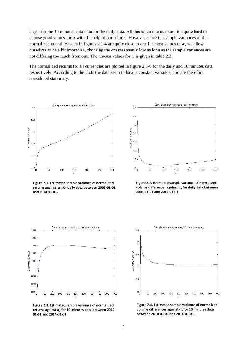
7

larger for the 10 minutes data than for the daily data. All this taken into account, it’s quite hard to

choose good values for with the help of our figures. However, since the sample variances of the

normalized quantities seen in figures 2.1-4 are quite close to one for most values of , we allow

ourselves to be a bit imprecise, choosing the :s reasonanly low as long as the sample variances are

not differing too much from one. The chosen values for is given in table 2.2.

The normalized returns for all currencies are plotted in figure 2.5-6 for the daily and 10 minutes data

respectively. According to the plots the data seem to have a constant variance, and are therefore

considered stationary.

Figure 2.1. Estimated sample variance of normalized returns against , for daily data between 2005-01-01 and 2014-01-01.

Figure 2.2. Estimated sample variance of normalized volume differences against , for daily data between 2005-01-01 and 2014-01-01.

Figure 2.3. Estimated sample variance of normalized returns against , for 10 minutes data between 2010-01-01 and 2014-01-01.

Figure 2.4. Estimated sample variance of normalized volume differences against , for 10 minutes data between 2010-01-01 and 2014-01-01.

8

Table 2.2. Chosen values of , for variance estimation on futures price returns.

Daily returns 16

Daily volumes 50

10 minutes returns 600

10 minutes volumes 600

Figure 2.5. Normalized daily returns between 2005-01-01 and 2014-01-01.

Figure 2.6. Normalized 10 minute returns between 2010-01-01 and 2014-01-01.

9

Transformation of spot data

As mentioned earlier, we are only considering weekly returns for the spot data in order to make the

causality assumption appropriate, since the prices are not synchronized.

As these are spot prices, which require an initial investment, we use logarithmic returns. As we want

to make use of our daily observations of open, high, low and close prices for estimating the variance

we stationarize the daily returns and are then considering the sum of daily returns between every

Wednesday. Conclusively, the quantities investigated in this case are:

∑

where and are the daily logarithmic returns and their estimated standard deviations the week

before . Usually, when the markets are open on all weekdays, we have 5 daily observations of returns

during one week. The standard deviations for daily returns are estimated by the Yang-Zhang measure

for logarithmic returns.

The forgetting factor, or , for estimating the variance is chosen in the same way as for the futures

data. However, the theoretical value of the sample variance should in this case be a bit less than 5,

since there usually are 5 daily observations within every week, and sometimes a little less. The sample

variance against the forgetting factor, for weekly returns is plotted in figure 2.7. We choose ,

which maximizes the sample variance around . The returns for all currencies are plotted in figure

2.8. Most currencies look stationary, whilst some still seem to have a bit non constant variance. We

assume, however, that the series are stationary in further analysis.

Figure 2.7. Estimated sample variance of returns against , for weekly data between 1994-07-01 and 2014-03-01.

10

Figure 2.8. Normalized weekly returns between 1994-07-01 and 2014-03-01.

11

2.3 Observations of predictive information

In order to find any patterns and predictive information in the data, it can be a good idea to study the

autocorrelations within the series of returns, as well as the cross correlations between currencies. In

order to be able to predict the return of a currency using this information, we will need significant

correlations at other lags than zero. If we consider the daily normalized returns between 2005-01-01

and 2014-01-01, we cannot observe any significant predictive information for any currency. We take

the New Zealand Dollar as an example, its Autocorrelation and Cross Correlation with the Japanese

Yen is plotted in figures 2.9-10.

The same quantities, but for weekly and 10 minutes returns respectively are plotted in figures 2.11-14.

For the 10 minutes data we can observe a significant negative autocorrelation at lag 1, and a positive

cross correlation with the Japanese Yen at lag . This means that the New Zealand dollar tends to

have a positive/negative return 10 minutes after a large negative/positive one in the same series and

also after a positive/negative one in the Japanese Yen. This can of course be used when speculating in

the New Zealand Dollar. For the weekly returns we cannot observe any predictive information

regarding the New Zealand Dollar. However, for the currencies of more developing countries, the

situation seems to be different. In figure 2.15 the Cross Correlation between the New Zealand Dollar

and the Thai Baht is plotted. We can observe a very significant positive cross correlation with lag 1 for

the Thai Baht, which means that the Thai Baht tend to have a positive/negative return one week after a

positive/negative return in the New Zealand Dollar. Similar patterns exist for several currencies of

developing countries. Another example is the Autocorrelation of the Indian Rupee, plotted in figure

2.16, which is significantly positive at both lag 1 and 2.

Figure 2.10. Cross Correlation between the New Zealand Dollar (positive lags on the negative axis) and the Japanese Yen (positive lags on the positive axis). Measured daily between 2005-01-01 and 2014-01-01.

Figure 2.9. Autocorrelation for the New Zealand Dollar. Measured daily between 2005-01-01 and 2014-01-01.

12

Figure 2.11. Autocorrelation for the New Zealand Dollar. Measured on 10 minutes intervals between 2010-01-01 and 2014-01-01.

Figure 2.12. Cross Correlation between the New Zealand Dollar (positive lags on the negative axis) and the Japanese Yen (positive lags on the positive axis). Measured on 10 minutes intervals between 2010-01-01 and 2014-01-01.

Figure 2.14. Cross Correlation between the New Zealand Dollar (positive lags on the negative axis) and the Japanese Yen (positive lags on the positive axis). Measured weekly between 1994-07-01 and 2014-03-01.

Figure 2.13. Autocorrelation for the New Zealand Dollar. Measured weekly between 1994-01-01 and 2014-03-01.

Figure 2.15. Cross Correlation between the New Zealand Dollar (positive lags on the negative axis) and the Thai Baht (positive lags on the positive axis). Measured weekly between 1994-07-01 and 2014-03-01.

Figure 2.16. Autocorrelation for the Indian Rupee. Measured weekly between 1994-01-01 and 2014-03-01.

13

Another interesting case to investigate is the cross correlation between the stationarized returns and

traded volumes during the intervals. For the ten minutes data the most interesting case is the cross

correlations between the Euro and its traded volume, which is plotted in figure 2.17. The same

quantity for the daily data is plotted in figure 2.18. We can observe a small significant negative

correlation at lag 1 in the 10 minutes data. This is the only significant observation in the 10 minutes

data, and there is none in the daily data at lag 1. The volume will be taken into account in one of our

models.

An insight after these observations is that there seem to be a lot more predictive information in the 10

minutes data compared to the daily data, at least for the major currencies whose data is measured in

futures prices. For the weekly spot returns, there seem to be some very significant predictive

information for the currencies of developing countries, but not for the major currencies. These

observations motivates why we only try to model the returns on 10 minutes and on weekly basis

respectively.

Figure 2.17. Cross Correlation between the Euro (positive lags on the negative axis) and its traded volume (positive lags on the positive axis). Measured on 10 minutes intervals between 2010-01-01 and 2014-01-01.

Figure 2.18. Cross Correlation between the Euro (positive lags on the negative axis) and its traded volume (positive lags on the positive axis). Measured daily between 2005-01-01 and 2014-01-01.

14

2.4 Distribution of the data

10 minute returns

The model distribution often used, for convenient reasons, is the normal distribution. However our

data of normalized returns on 10 minute bars does not really seem normal distributed. The prices most

often do not move very drastically on periods of 10 minutes, which commonly only gives us one or

two significant figures for the returns, and also many zero-observations (often above 10 % of the

cases). The normalized returns seem to have a smaller full width at half maximum (FWHM) and also

heavier tails than the normal distribution. These observations might suggest either a discrete

distribution or a student’s t-distribution as better alternatives. See figure 2.19 and 2.20 for Quantile-

Quantile plots of the seven currencies vs. the Normal distribution and the Student’s t-distribution

respectively. From the figures we can draw the conclusion that a Normal distribution isn’t optimal,

and that the Student’s t-distribution indeed fits much better for all currencies.

Even if the assumption of a normal distribution seems to be suboptimal, we are still going to use it in

some models. This is explained by much more convenient modeling, especially in the Bayesian case.

However, this is something that could be interesting to improve in future research.

Figure 2.19. Quantile-Quantile plots for the 10 minutes returns versus the Normal distribution. Data from a perfect Normal distribution should follow the dotted line. The returns are measured on 10 minutes intervals between 2010-01-01 and 2014-01-01.

15

Weekly returns

One reason to try out weekly returns in our modeling, besides involving a broader range of currencies,

is that the prices can be expected to move more on longer horizons, and thereby the continuous

assumption of the returns is more appropriate. In figure 2.21 Quantile-Quantile plots for all weekly

currency returns are plotted against the Normal distribution. One can see that the assumption of a

Normal distribution seems much more appropriate in the case of weekly returns for most currencies.

The questionable currencies are especially the Indonesian Rupiah (IDR), and maybe also the Indian

Rupee (INR).

Figure 2.20. Quantile-Quantile plots for the 10 minutes returns versus the Student’s t-distribution. Data from a perfect t-distribution should follow the dotted line. The returns are measured on 10 minutes intervals between 2010-01-01 and 2014-01-01. The degrees of freedom of the fitted t-distributions are: 4.31, 3.93, 3.23, 3.41, 3.87, 3.07 and 4.34 for the AUD, CAD, CHF, EUR, GBP, JPY and NZD respectively.

16

Figure 2.21. Quantile-Quantile plots for the weekly spot returns versus the Normal distribution. Data from a perfect Normal distribution should follow the dotted line. The returns are measured weekly between 1994-07-01 and 2014-03-01.

17

3. Forecasting models

The problem of modeling the normalized returns can be attacked in a lot of different ways. A broad

range of models have been tried in order to make a comparison, and thereafter be able to choose the

best performing model for further analysis.

In some models one has to make distributional assumptions on the data, and often the normal

distribution is the most convenient one to use. This has been shown to be suboptimal for the 10 minute

returns, but more appropriate for the weekly returns.

3.1 Bayesian modeling

If one has some prior beliefs about the data, or most importantly in order to avoid overfitting to certain

training samples, one can use a Bayesian approach, and “shrink” the model parameters in the direction

of those corresponding to the prior beliefs. The approach aims at reducing the total prediction error by

a lower variance of the estimators, but with the price of a higher systematic error called the bias. A

more throughout explanation of this is given in 5.1.

Bayesian inference has got its name after Bayes’ rule:

( | ) ( )

( )

( | ) ( )

( )

where and are arbitrary random variables. When modeling, one often uses Bayes’ rule with as

the observed data, ,and as the distributional parameters which one wants to

estimate. One often uses the terms “prior” for ( ), “likelihood” for ( | ) and “posterior” for

( | ). Notice that ( | ) is the likelihood one often wants to maximize in the frequentist approach

to inference. ( ) is not very relevant in the case of Bayesian inference, since this term is not a

function of the parameters, , and therefore is only part of a normalizing constant in the

density/probability function of the parameters, i.e. one can often derive the posterior distribution

without knowledge about the unconditional distribution of the data.

In order to use Bayes’ rule in this way one has to specify a prior distribution for the parameters. One

can do this very freely, but there are choices that are more convenient than others. A common

approach is to choose the prior such that the posterior belongs to the same family of probability

distributions. These are called conjugate priors, and often make the posterior much easier to derive.

(Robert, 2001, pp. 113-120). It is also quite intuitive to assume that the parameters belong to one

family of distributions, which stays the same also after observations of the data. Conjugate priors are

often parameterized distributions, for example: ( ) ( ), where and can be the prior

mean and standard deviation. These are called hyperparameters, and need to be specified, which allow

for incorporating prior beliefs, or “shrinkage”.

If one does not have any prior beliefs about either distributions or hyperparameters, one can use an

uninformative prior. One alternative is to choose the prior as a constant; ( ) , then:

( | ) ( | )

However, this might not be invariant under reparametrization, which means that if we reparametrize

the random variables , we might get another prior distribution than the one we suggested. One can

show (by the change of variable theorem) that a prior that is invariant under reparametrization is:

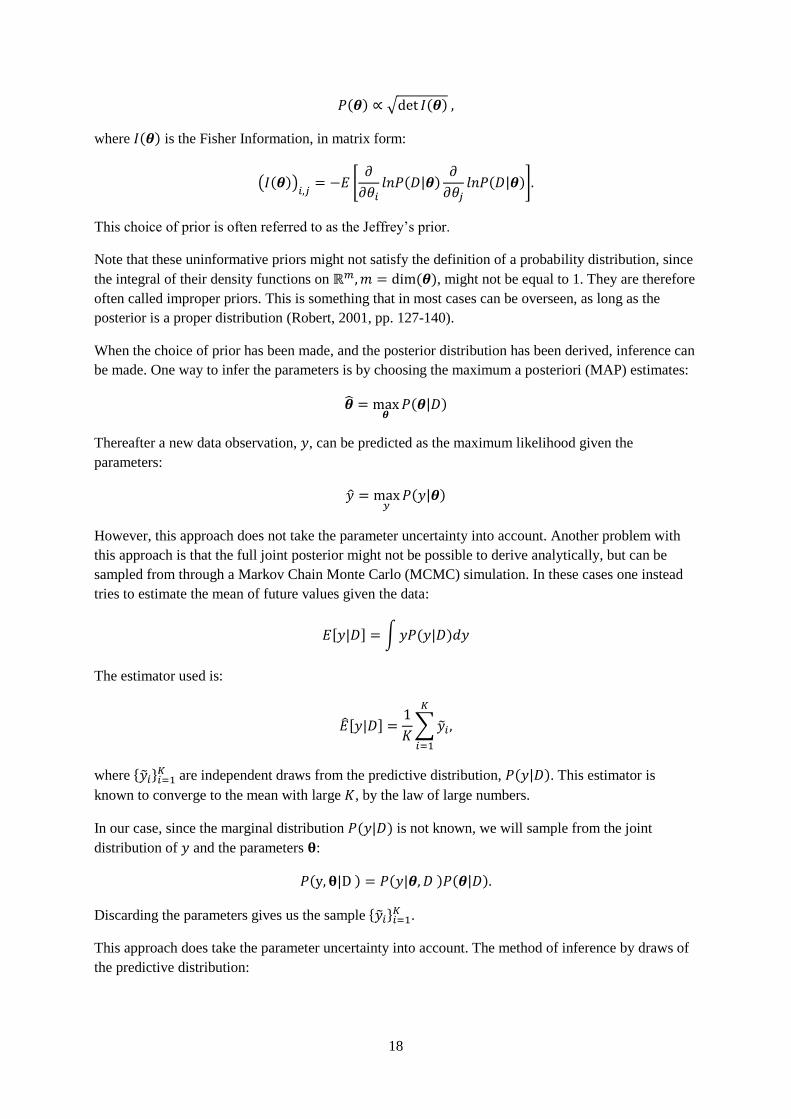
18

( ) √ ( )

where ( ) is the Fisher Information, in matrix form:

( ( ))

[

( | )

( | )]

This choice of prior is often referred to as the Jeffrey’s prior.

Note that these uninformative priors might not satisfy the definition of a probability distribution, since

the integral of their density functions on ( ), might not be equal to 1. They are therefore

often called improper priors. This is something that in most cases can be overseen, as long as the

posterior is a proper distribution (Robert, 2001, pp. 127-140).

When the choice of prior has been made, and the posterior distribution has been derived, inference can

be made. One way to infer the parameters is by choosing the maximum a posteriori (MAP) estimates:

( | )

Thereafter a new data observation, , can be predicted as the maximum likelihood given the

parameters:

( | )

However, this approach does not take the parameter uncertainty into account. Another problem with

this approach is that the full joint posterior might not be possible to derive analytically, but can be

sampled from through a Markov Chain Monte Carlo (MCMC) simulation. In these cases one instead

tries to estimate the mean of future values given the data:

[ | ] ∫ ( | )

The estimator used is:

[ | ]

∑

where are independent draws from the predictive distribution, ( | ). This estimator is

known to converge to the mean with large , by the law of large numbers.

In our case, since the marginal distribution ( | ) is not known, we will sample from the joint

distribution of and the parameters :

( | ) ( | ) ( | )

Discarding the parameters gives us the sample .

This approach does take the parameter uncertainty into account. The method of inference by draws of

the predictive distribution:

19

( | ) ∫ ( | ) ( | )

is known as Bayesian model averaging (BMA).

The main idea behind MCMC methods is to find a Markov chain with the same stationary distribution

as the distribution one wants to sample from.

In our case we have the model distribution, ( | ), at hand. However the posterior joint

distribution for the parameters, ( | ), might be unknown. Suppose that we can derive the

conditional posteriors, ( | ) ( | ) where is the dimension of , and

. Then we can use a so called Gibbs sampler, given in algorithm 3.1. It can be shown

that this Gibbs sampler has ( | ) as its stationary distribution. However it may take some samples

for it to converge, and one should therefore use a burn in, ignoring some number of samples at the

beginning. The generated samples are not independent, since the sequence of parameters has the

Markov property, and do therefore depend on the most recent update. This is often ignored, or solved

by only saving every th sample, for a predetermined value of (Robert, 2001, pp. 307-309).

1. Initialize ( )

2. For j=1, …, K:

- Draw ( )

( | ( )

( )

( )

( )

)

for each .

- Draw ( | ( ) )

3. Save the samples, { }

, and discard the parameters.

Algorithm 3.1. General Gibbs Sampler, to sample from the predictive distribution:

( | ) ∫ ( | ) ( | )

20

3.2 Time series models

General VAR model

A Vector Autoregressive (VAR) model of order generally has the form:

∑

where is the -dimensional vector of normalized returns at time , a -dimensional vector of

exogenous variables, e.g. historical trading volumes, deterministic constants etc.,

[

] a dimensional vector, [ ] a matrix and

errors ( ) a white noise process. This implies:

( )

If we collect values for all times up to , we can write:

[

] [

] [

]

The parameters, , and the covariance matrix of the noise, , can be estimated by ordinary least

squares as

( )

where ( ) ( ) is the residual sum of squares (RSS) and are the degrees of

freedom. In non-dynamic regression problems, these estimators are known as the minimum variance

unbiased estimators. In time series models they are generally not unbiased, but we can expect a much

lower bias using this approach compared to the Bayesian models suggested below.

Future returns can be estimated as:

[

] ∑

∑

or, more compact, if :

[

]

21

Bayesian VAR model

Currencies behave very random, which implies that our model is very sensitive to overfitting, and a

too complex model can ruin the predictions completely by a too high variance. In order to improve our

results we want to incorporate prior beliefs, and thereby introduce some bias in order to reduce the

variance.

The Bayesian VAR model used is the one with a so called Normal-Wishart prior suggested by

Karlsson in the working paper Forecasting with Bayesian Vector Autoregressions (Karlsson, 2012, pp.

16-17). An explanation of the model is given below.

To be able to incorporate any beliefs, we need to specify a prior distribution on the parameters , as

well as on the error covariance matrix, . As it is hard to specify any prior beliefs about the errors, we

specify an improper Jeffrey’s prior for , while we specify the natural conjugate prior for the

vectorization of the parameters, ( ), which is the normal distribution. To be specific, we

choose the prior distributions:

( )

( ) √ ( )

where and are hyperparameters for the prior mean and covariance matrix of the parameters. We

also, a priori, assume independence between and .

As in the general VAR model, we have ( ). The posterior distributions are derived

through Bayes theorem:

( | ) ( | ) ( )

( ) ( | ) ( )

Since we a priori assume independence:

( ) ( ) ( )

we can state the conditional posteriors:

( | ) ( | ) ( | ) ( )

( | ) ( | ) ( | ) ( )

22

For the likelihood we have:

( | ) ( )

{

∑ (

) (

)

}

( )

{

[( ) ( ) ]}

( )

{

[ ( ) ( )]}

( )

{

[ ( )

( )]}

{

[ ( )

( )]}

where is the least squares estimate, and the operation ( ) is the trace of the matrix . With

( ) and ( ), we can write:

[ ( ) ( )] ( )

( )( )

where is the Kronecker product.

Now we get:

( | ) {

( )

( )( )} {

( )

( )}

This can be written as:

( | ) {

( )

( )}

where:

( )

[ ( ) ]

We recognize this as the normal distribution, and we can therefore state the conditional posterior for ,

as:

| ( ) (1)

The conditional posterior for follows directly from the likelihood:

( | ) {

[ ( ) ( )]}

{

[ ]}

This is recognized as the inverse Wishart distribution:

| ( ) (2)

23

( ) ( )

The inverse Wishart distribution is the multivariate extension of the inverse gamma distribution, which

is the conjugate prior for the variance in a univariate normal distribution.

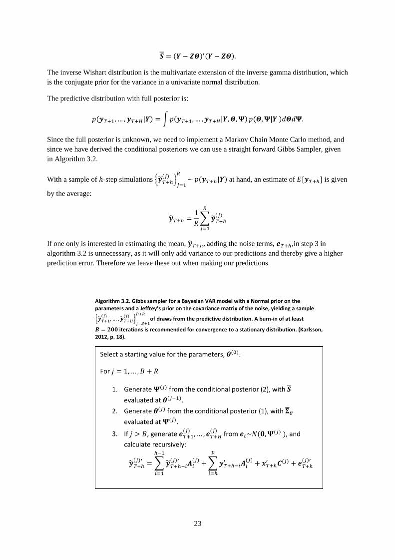
The predictive distribution with full posterior is:

( | ) ∫ ( | ) ( | )

Since the full posterior is unknown, we need to implement a Markov Chain Monte Carlo method, and

since we have derived the conditional posteriors we can use a straight forward Gibbs Sampler, given

in Algorithm 3.2.

With a sample of -step simulations { ( )

}

( | ) at hand, an estimate of [ ] is given

by the average:

∑

( )

If one only is interested in estimating the mean, adding the noise terms, ,in step 3 in

algorithm 3.2 is unnecessary, as it will only add variance to our predictions and thereby give a higher

prediction error. Therefore we leave these out when making our predictions.

( )

∑ ( )

( )

∑

( )

( )

( )

Select a starting value for the parameters, ( ).

For

1. Generate ( ) from the conditional posterior (2), with

evaluated at ( ).

2. Generate ( ) from the conditional posterior (1), with

evaluated at ( ).

3. If , generate ( )

( )

from ( ( ) ), and

calculate recursively:

Algorithm 3.2. Gibbs sampler for a Bayesian VAR model with a Normal prior on the parameters and a Jeffrey’s prior on the covariance matrix of the noise, yielding a sample

{ ( )

( )

}

of draws from the predictive distribution. A burn-in of at least

iterations is recommended for convergence to a stationary distribution. (Karlsson, 2012, p. 18).

24

Choice of hyperparameters

When specifying the hyperparameters, and , we want to incorporate some prior beliefs of our

data. As currencies often are believed to behave like random walks, it is a good idea to shrink our

model to those beliefs. This was first done (with other economic variables) by Robert Litterman

(Litterman, 1979). If the currency prices behave like univariate random walks, it means that their

returns behave like Gaussian noise, i.e. ( ). In order to shrink our model in this

direction, we put the prior mean for the elements of to:

( ) [( ) ]

We want to apply more shrinkage (i.e. specify a smaller prior variance) to lags of independent

covariate variables, as well as to larger lags than to small. A modification of the original Litterman

prior is the following, for the standard deviations of the elements of :

( ) [( ) ]

{

( )

( )

( )

where are the diagonal elements of the least squares estimate of the residual covariance matrix

,

so that accounts for the different variances of the variables. is a hyperparameter for the

“overall tightness”. , and control the tightness for independent variables, different lags and

exogenous variables (e.g. traded volumes) respectively.

Then we specify ( ) and as the diagonal matrix of ( ), i.e.:

( ([( ) ]))

which implies that the parameters get the specified prior variances, and that we assume no prior

covariance between different parameters.

3.3 Markov models

General Markov model

One way to exploit the observation about the negative autocorrelation at lag 1 (or higher lags if

desired) for the 10 minutes data, without making the normality assumption, is by modeling the returns

with a Markov model. The model suggested will however not take any notice to correlations between

currencies or with volumes, in order to keep the number of Markov states reasonably limited.

In this model, the state at time will represent how big/small return that is observed at time . The

positive and negative returns are divided evenly in different states each, i.e. as quantiles of the

data (and thereby get an even number of states, ,in total). With this approach we can estimate the

transition probabilities for observing a large positive return in 10 minutes given a large negative return

in the present etc. We can also just estimate the probability of a positive/negative return given the

present state in general.

Define the different states as:

25

In this case corresponds to different intervals of negative and positive returns respectively. Let the

state at time be given as . The transition probabilities for a Markov chain of order are then

defined as:

( | )

where . The corresponding transition matrix is:

[

]

The transition probabilities can be estimated by maximum likelihood as:

∑

where is the number of observed transitions in the order of states: .

With the estimated transition probabilities for the states of returns at hand, it is straightforward to

estimate the probability of a specific future state, and also for simply a positive/negative return. The

estimate for the probability of a positive return is:

∑

where corresponds to states of positive returns. The probability of a negative return is estimated in

the same way:

∑

where corresponds to states of negative returns.

Bayesian Markov model

A Bayesian approach for general, observable, Markov chains is to assume a multinomial distribution

for the occurrences, i.e. for transitions from any fixed path of length , , to state :

( )

where ( ) are the transition probabilities to states .

The probability mass function of the multinomial distribution is:

( ) {

∏

∑

26

The conjugate prior for the probabilities in the multinomial distribution is the Dirichlet distribution:

( )

where the hyperparameters ( ) are the prior occurrences of transitions to states

(Robert, 2001, p. 121).

The density function of the Dirichlet distribution is:

( ) ∏ ( )

(∑ )

∏

It is easy to derive the posterior. Using Bayes’ rule:

( | ) ( ) ∏

which can be identified as a new Dirichlet distribution, and it is proved that the Dirichlet distribution

indeed is the conjugate prior. Conclusively, the posterior is:

| ( )

with the conditional mean and variance:

[ | ]

[ | ] ( )( ( ))

( )

where ∑ ( ).

This approach allows us to shrink the transition probabilities towards 1/N, which means that all states

are equally probable. This is done by choosing , the larger we choose them, the

more shrinkage is applied.

When modeling, the transition probabilities are simply estimated by their posterior means:

Note that this is done for all possible paths, , to state , those are just left out from the sub-

indexes for a more convenient notation.

As we are only interested in shrinking the model towards equally probable states, we only get one

hyperparameter:

27

3.4 Making predictions

For the VAR model, predictions can be made in a very straightforward way, since we are actually

estimating the mean of future returns, . However, if we are only interested in predicting whether the

return is going to be positive or negative, and only want to have an opinion about this at times where

we consider ourselves reasonably certain about the outcome, for example in order to make a trade.

Then we can try to predict the sign of the returns as follows:

( ) {

where is a threshold that the predictions need to exceed in order to have an opinion about a

positive/negative return. Only the case with will be considered under the results in 7.1.

For the Markov models, since we do not have any predicted values of returns, but only transition

probabilities corresponding to different states of positive/negative returns, a similar approach is

conducted in all cases:

( ) {

( | )

( | )

where is a threshold that the transition probability corresponding to a positive/negative state

needs to exceed in order to have an opinion.

3.5 Updating the models

Even if we have assumed stationarity, the correlation structure within or between the return series

might be time dependent. We want dynamic models that are able to adapt to these changes over time,

therefore we are not only training the models on specific previous samples of data, but are updating

them over time, when new samples are observed. To do this, we choose a number of previous samples

that our model is trained on and either update our model at every iteration, or choosing a frequency of

how often the model is updated, i.e. the model is updated every :th iteration using previous data

points. The choice of updating frequency depends on the computational complexity of the model.

Updating the models at every iteration can take a lot of time, especially when validating the models in

order to specify hyperparameters. The number of previous samples to be used for training, , is

regarded as a hyperparameter chosen by out of sample validation.

28

4. Trading strategies

When having predictions of future returns we need to specify when we want to trade, and what

currencies to trade during certain time intervals. An intuitive way to trig the trades is to specify

suitable thresholds for the predicted return or (for the Markov models) a threshold for the estimated

probability of negative/positive return in the next state.

When we’ve come up with suitable FX rates to trade during a certain interval, then we need to know

how much we should go long/short in each currency. To do this we use the modern portfolio theory

(MPT) suggested by Harry Markovitz (Wikipedia, MPT, 2014).

4.1 Portfolio theory

The main idea of MPT is to maximize our portfolio’s expected return:

[ ]

where ( ), [ ], are the expected returns on the traded markets, and is the

weights for the assets of the portfolio.

At the same time we don’t want to take too high risks, which mean that we need a limit for the

variance of the portfolio:

[ ]

where is the covariance matrix of the returns.

This can be stated as the following optimization problem:

This problem can be rewritten as:

( ) ( ) ( )

where is a Lagrange multiplier. The gradient w.r.t the weights is:

( )

Setting the gradient equals to zero gives us the solution:

The analysis will be based on the normalized returns, which each should follow processes of zero

mean and unit variance, which implies that the covariance matrix is the same as the correlation matrix.

We use the weights

, where will be our predictions of normalized returns at time ,

and the sample covariance matrix for the previously observed normalized returns, which with zero

mean is:

29

( ) ∑

Where are the vectors of normalized returns at time .

With weights at hand we can test our model and estimate the expected returns and standard deviation

for the portfolio. To do this, we should also take the transaction costs into account. If we assume that

the transaction costs are constant, for all FX rates, we get the portfolio return at time as:

∑

∑| |

VAR models

For the VAR models we can use the MPT very straightforward as:

Where is our predictions of stationarized returns at time , when all information up to time

can be observed.

Markov models

In the Markov models we estimate transition probabilities from the current state to a state

corresponding to a positive/negative return. Therefore we will not have predictions of the mean of the

future returns, and cannot use MPT in the same straightforward way as for the VAR models. However,

we can make predictions of the sign of returns, and are simply putting:

{ ( | )

( | )

With the sign-predictions at hand, the weights are computed as before:

30

5. Performance measures

In order to validate our models and be able to tell whether their predictions are good or not, we will

need performance measures. The ones used are the root mean squared error (RMSE), when we are

predicting values of the returns as in the VAR models, and the hit rate when we only try to predict

whether future returns are expected to be positive or negative. In order to evaluate the trading

strategies, we use the Sharpe ratio as the performance measure.

5.1 Root mean squared error

The most common performance measure in regression is the mean squared error (MSE), and its square

root (RMSE). The MSE is often also referred to as the “loss function” one want to minimize by the

regression. The MSE for the prediction of the dependent variable is defined as:

( ) [( ) ]

In order to minimize the MSE, one is often referring to the problem of finding an optimal trade-off

between bias and variance. This is where the Bayesian modeling comes into place, where one

incorporate prior beliefs for the model parameters. This results in a lower variance of the estimator,

but also introduces a systematic error between the estimator and the dependent variable, i.e. the bias.

With this approach one can reduce the total expected error compared to the unbiased estimators, e.g.

ordinary least squares in the case of regression.

To get a better understanding about the tradeoff between bias and variance, we prove the fact that the

MSE can be decomposed in three terms: the variance of the estimator, the squared bias of the

estimator and the variance of the so called innovation.

One can think of as an estimate of [ ], the true mean value of given all information known at the

moment when the estimate is made. The bias can then be defined as the difference between the mean

of the chosen estimator and [ ], i.e. a systematic error in the model. Consider the term [ ],

generally called the innovation. It has zero mean and is uncorrelated with and [ ].

The decomposition of the MSE can be done as follows:

( ) [( ) ]

[( [ ] ) ]

[ ] [( [ ]) ]

( ) [( [ ]) ]

since the innovation, , has zero mean and is uncorrelated with ( [ ]). In the second term, we add

and subtract [ ], which is the true mean of the prediction, i.e. the average prediction with infinitely

many replications of the training data.

[( [ ]) ]

[( [ ] [ ] [ ]) ]

[( [ ]) ] [( [ ] [ ]) ] [( [ ])( [ ] [ ])]

31

[( [ ]) ] ( [ ] [ ])

( ) ( )

since ( [ ] [ ]) is a constant and [ [ ]] [ ] [ ] Conclusively:

( ) ( ) ( ) ( )

With the observed values: , and the corresponding predictions: , the MSE is

estimated as:

( )

∑( )

In order to get the same scale as the quantity predicted, we use the square root:

( ) √

∑( )

A common way to get an idea of the prediction accuracy for financial data is to compare the result

with the one of a random walk-model for the prices, i.e. setting the mean of the returns to zero, and we

get the RMSE:

√

∑( )

5.2 Hit Rate

In some cases it can be more interesting to investigate how often we are able to predict the correct sign

of the returns. In these cases we use the hit rate as the performance measure:

∑ ( ) ( )

Since we have a lot of zero observations of returns (especially in the 10 minutes data), we only count

those that are strictly positive or negative when computing the hit rate. This is reasonable, since we

only try to predict positive and negative signs, and we doesn’t really lose money on a zero return, at

least not if the transaction costs are omitted.

For the hit rate we can estimate a confidence interval to investigate if the hit rate is significantly better

than , i.e. if we can predict the signs of positive/negative returns better than random.

With the assumption that the hit rate is independent in time, we can put:

∑ ( ) ( )

( )

which gives us:

32

∑ ( ) ( )

The standard deviation of the hit rate is estimated as:

√ ( )

Then a confidence interval can be estimated as:

where is the (

) th percentile of the standard normal distribution, 1.645, 1.96 and 2.58

for the 95, 97.5 and 99.5 percentiles respectively.

5.3 Sharpe ratio

The Sharpe ratio will be used as the performance measure for our trading strategies, and is indeed used

in reality by investors comparing the performance of different portfolio managers.

As mentioned in 4.1, a good trading strategy yields a high positive return, but also doesn’t take too

much risk, measured by the standard deviation (volatility). We define the (yearly) Sharpe ratio as:

[ ]

where [ ] and its standard deviation, usually are measured on a yearly basis, and can simply be

estimated by the average and the sample variance respectively. In many definitions the Sharpe ratio

also contains a term for the risk free interest rate, which is omitted in this case. For 10 minutes/weekly

data, if one assumes that the returns are uncorrelated during different intervals, we get the yearly

Sharpe ratio:

[ ]

√

√

[ ]

where the returns and standard deviation in this case are measured on 10-minutes or weekly intervals,

and is the number of 10-minutes/weekly intervals traded during a year. In our case 38 10 minutes

intervals during approximately 252 trading days makes for the 10 minutes data. As there

are 52 weeks per year and we are trading every week, for the weekly data.

33

6. Model specifications

There are a lot of different choices that have to be made when specifying the models. The orders of the

VAR models and Markov chains have to be selected, the different hyperparameters have to be chosen

etc. There are theoretical ways to specifying the model orders, while the hyperparameters often need to

be specified through empirical studies of the results while back testing.

6.1 Training, validation and test sets

In order to not overfit our specifications to one sample of data points we use a limited data set for the

specifications, in order to save a sample for evaluating our models when all specifications have been

made. Usually one divides the data in three different data sets: training, validation and test sets. The

training set often refers to a set where one “trains” a model using a specific model specification.

Thereafter one validates the model on the validation set, and chooses the specification that gives the

best results. In order to not overfit the model to the validation set one evaluates the model on the

previously unused test set. If the model performs well on the test set, one expects the model to perform

well even in the future, for presently unobserved data.

As we have chosen a dynamical approach to update our models the training sets will change over time,

while new observations are made. However, we divide our data in a sample for training and validation,

and a test set for evaluation and comparison of the models.

For the data of 10 minute returns we choose the train/validation set as 25 000 observations between

2010-06-01 and 2012-08-01, and the test set as 13549 observations between 2012-08-01 and 2013-12-

30.

For the data of weekly returns we have a lot less observations. We choose the train/validation set as

700 observations between 1995-06-09 and 2008-10-31, and the test set as 280 observations between

2008-11-07 and 2014-03-14.

All data in the train/validation set might not always be used for training and validation, since the

model complexity might be too high for validating several different choices of model specifications.

The most important part is that we want to separate the test and train/validation sets in order to avoid

overfitting and be able to test our models on a previously unused sample of data.

34

6.2 Order Selection

To select the order of the time series and Markov chain models, we use the Bayesian information

criterion (BIC) as well as the Akaike information criterion (AIC):

where is the estimated maximum likelihood of the model, is the number of free parameters to be

estimated and is the number of data points. (Wikipedia, AIC, 2014), (Wikipedia, BIC, 2014).

The idea of both measures is to select an optimal model with respect to goodness of fit as well as the

complexity of the model. Having a lot of parameters make the model more complex, which might

result in overfit to the training data.

The model to select is the one with the smallest AIC/BIC. However, these measures can be in conflict

with each other, BIC generally tends to penalize many parameters more heavily than AIC.

General VAR

In the general VAR model, we have that:

( )

The corresponding multivariate normal density function is:

√( ) ( ) {

[

] [ ]}

Taking the product for all up to , evaluating at the maximum likelihood estimates given under the

general VAR model and then taking the logarithm, yields the maximum log likelihood:

( ( ))

∑[

] [

]

The number of free parameters is the sum of the elements in and the free parameters of :

( )

The AIC and BIC for a general VAR model of order 1-4 is presented in table 6.1 for 10 minutes

returns, and in table 6.2 for the weekly returns. The models do not contain any exogenous variables,

such as volumes. For the weekly returns both AIC and BIC suggests order 1, but for the 10 minutes

returns AIC suggests order 2 while BIC suggests order 1. We will only investigate the case of order 1,

since the margin between order 1 and 2 for BIC is considered large.

35

Table 6.1. AIC and BIC for 10 minutes returns modeled by a general VAR model of orders 1-4.

Order AIC BIC

1 399 403 400 122

2 399 362 400 500

3 399 372 400 930

4 399 386 401 363

Table 6.2. AIC and BIC for weekly returns modeled by a general VAR model of orders 1-4.

Order AIC BIC

1 56 217 59 927

2 56 604 62 679

3 56 960 65 401

4 57 368 68 174

Bayesian VAR

The AIC and BIC tests for the general VAR gives us a hint of what orders to use also in the Bayesian

case. However, as we are able to shrink parameters corresponding to lags of higher orders more than

those of low orders; we at least want to try one model of a bit higher order than one. We also want to

investigate the results when the traded volumes are taken into account. The Bayesian VAR models

investigated, both for weekly and 10 minute returns, are:

1. Bayesian VAR of order 1 without exogenous variables, called VAR1.

2. Bayesian VAR of order 1 with traded volumes as exogenous variables, called VARX1.

3. Bayesian VAR of order 4 without exogenous variables, called VAR4.

Markov Models

For a first order Markov chain the likelihood function is derived as:

( ) ( ) ( | ) ( | )

( )∏

( )∏∏

This gives us the maximum log likelihood:

( ) ∑ ∑

where are the maximum likelihood estimates of the transition probabilities. The term (

) is often left out, since it’s small compared to the other term when we have a lot of observations.

For a Markov chain of order , the log likelihood is:

( ) ( ) ∑ ∑ ∑

36

where the terms ( ) ( ) can be left out if we have a lot of observations.

The number of free parameters is:

( )

since we have rows in the transition matrix, and possible transitions with the constraint

∑ .

Before choosing the order of the Markov chains, we need to specify how many states we should have.

This can also be done by AIC/BIC, but since we want to get as significant probabilities for

positive/negative returns as possible, we shouldn’t have less than four states (two for positive/negative

returns respectively). The AIC/BIC measures for Markov chains with four and six states, for all

currencies, of order 0-3 are presented in table 6.3-9.

We notice that the BIC always suggests the model of order 1, while AIC suggests the model of order 2

in all cases but for the Swiss franc. Since the difference in BIC between order 1 and 2 is more

significant than for AIC, and because of the convenience of having the same order for all currencies,

we choose to model all currencies with the first order Markov chain.

If we do the same procedure for weekly returns, BIC suggests order 0 for all currencies and AIC

suggests order 1 only for a few. This indicates that the Markov models are not appropriate for the

weekly returns. We will therefore only consider 10 minute returns in the Markov models.

Conclusively we choose the following Markov models, both in the general and in the Bayesian case:

1. 1:st order Markov model of 4 states.

2. 1:st order Markov model of 6 states.

Table 6.3. Markov model for AUD. AIC and BIC for 4 and 6 states, of orders 0-3.

Order 0 Order 1 Order 2 Order 3

AIC 4 states 64 710 64 541 64 491 64 578

6 states 83 640 83 422 83 409 84 203

BIC 4 states 64 734 64 638 64 878 66 125

6 states 83 680 83 664 84 860 92 906

Table 6.4. Markov model for CAD. AIC and BIC for 4 and 6 states, of orders 0-3.

Order 0 Order 1 Order 2 Order 3

AIC 4 states 64 042 63 863 63 782 63 835

6 states 82 775 82 477 82 444 83 238

BIC 4 states 64 066 63 959 64 168 65 380

6 states 82 815 82 718 83 893 91 929

37

Table 2.5. Markov model for CHF. AIC and BIC for 4 and 6 states, of orders 0-3.

Order 0 Order 1 Order 2 Order 3

AIC 4 states 64 363 64 072 64 020 64 089

6 states 83 191 82 743 82 750 83 512

BIC 4 states 64 387 64 168 64 406 65 635

6 states 83 231 82 985 84 200 92 208

Table 6.6. Markov model for EUR. AIC and BIC for 4 and 6 states, of orders 0-3.

Order 0 Order 1 Order 2 Order 3

AIC 4 states 65 333 65 089 64 969 65 031

6 states 84 444 84 121 84 055 84 812

BIC 4 states 65 357 65 186 65 356 66 580

6 states 84 484 84 363 85 507 93 525

Table 6.7. Markov model for GBP. AIC and BIC for 4 and 6 states, of orders 0-3.

Order 0 Order 1 Order 2 Order 3

AIC 4 states 65 156 64 898 64 830 64 867

6 states 84 215 83 868 83 853 84 697

BIC 4 states 65 180 64 994 65 218 66 415

6 states 84 256 84 110 85 305 93 407

Table 6.8. Markov model for JPY. AIC and BIC for 4 and 6 states, of orders 0-3.

Order 0 Order 1 Order 2 Order 3

AIC 4 states 63 227 62 818 62 688 62 715

6 states 81 721 81 017 80 939 81 578

BIC 4 states 63 251 62 914 63 074 64 258

6 states 81 762 81 258 82 385 90 256

Table 6.9. Markov model for NZD. AIC and BIC for 4 and 6 states, of orders 0-3.

Order 0 Order 1 Order 2 Order 3

AIC 4 states 64 152 63 931 63 888 63 956

6 states 82 917 82 559 82 600 83 480

BIC 4 states 64 176 64 028 64 275 65 502

6 states 82 958 82 800 84 049 92 173

38

6.3 Specifying hyperparameters

In the Bayesian models, there are a lot of different hyperparameters that need to be specified. As

mentioned earlier, some are chosen by prior beliefs about the data, while some have to be chosen in

some more empirical way.

In order to specify the hyperparameters we validate the model on samples of data within the

training/validation data sets. This can take a lot of time depending on the computational complexity of

the model. In some cases we choose to only update the model with a specified iteration frequency, in

order to reduce computation time. This might not give us as good prediction results as when updating

at every iteration, but should be sufficient to indicate preferred values on the hyperparameters. Later,

when testing our specified models, we will update the models at every iteration.

Another approach to save time is to run the algorithms in parallel, using the computational power of

several machines. This is done for the Bayesian VAR models, where we use a parallel loop to evaluate

the models for different combinations of hyperparameters.

General VAR

In the general VAR model the parameters are estimated by least squares, and do therefore not require

any hyperparameters. However, we need to specify how large training sample to use. To save time, we

choose to update our model every 10:th iteration for the weekly data, and every 50:th iteration for the

10 minute data.

For the weekly data, we validate the model for different values of on the last 200 observations in the

train/validation set, and for the 10 minutes data we validate on the last 1000 observations of the

train/validation set. The average MSE for the different return series against is plotted in figure 6.1-2

for the weekly and 10 minutes returns respectively. In the figures, we notice that the MSE is

decreasing with . We can draw the conclusion that one should use as large training sample as

possible in the general VAR model, i.e. we choose to train on all previous observations.

Figure 6.1 Average MSE against the number of training samples used, , when validating on 200 observations of weekly returns.

Figure 6.2 Average MSE against the number of training samples used, , when validating on 1000 observations of 10 minute returns.

39

Bayesian VAR

In the Bayesian VAR models we need to specify the hyperparameters , , and mentioned

under the description of the Bayesian VAR model. We also need to specify the number of previous

observations to train our models on, .

The chosen approach is to randomly pick 1000 combinations of the hyperparameters at reasonably

specified intervals, and validate the models for 4 randomly chosen currencies (in each iteration) on the

500 and 200 latest observations in the train/validation set for the 10 minutes and weekly observations

of returns respectively. Then we use Nadaraya-Watson kernel regression to fit a curve for the average

MSE of all currencies against the different hyperparameters. With this approach we can plot the

average MSE for the currencies involved against any individual hyperparameter, and also under

smaller intervals of other hyperparameters.

Nadaraya-Watson estimates the conditional mean of a random variable , given covariates :

[ | ] ∫ ( | ) ∫ ( )

( )

where ( ) is the marginal density function of , and ( ) is the joint density function of and .

(Powell, 2008). In our case Y is the MSE and X is the hyperparameters. The density functions are

estimated by so called kernel density estimation, where we use a Gaussian kernel and a suggested

optimal bandwidth (Bowman & Azzalini, 1997, p. 31).

With the plots of MSE’s against hyperparameters at hand we want to choose the hyperparameters so

that the MSE is minimized. However, as will be noted, there is a lot of variance in our data, which

often implies that there is no perfect minimum, and that the choices might be quite arbitrary.

When validating the models, we use a cluster of machines to parallelize the MSE calculations for

different combinations of parameters. With the configuration used it still takes several hours to

perform the validation for 1000 combinations. We are updating the models in each iteration, since this

step takes far less time than the Monte Carlo simulation performed in the prediction step.

10 minute returns

For the 10 minute data, we will select the hyperparameters in the following order:

1. Select

2. Select and under a shortened interval of

3. Select from a new validation under the other specified hyperparameters.

It is quite intuitive that we first select , which accounts for the “overall tightness”, and then select

the parameters controlling the tightness of independent variables, different lags and exogenous

variables (e.g. traded volumes) respectively, which indeed should be dependent of , but

approximately independent of each other. Lastly we select , which should be dependent on how

much shrinkage that is applied to the parameters. With a large the model mostly rely on patterns

within the whole sample to not overfit the model, while we with a high regularization and a smaller

might be able to catch time dependent patterns and dependencies without overfitting the model.

In figure 6.3, 6.5, and 6.8 the average MSE’s are plotted and regressed against for the different

Bayesian VAR models. We will choose as the minimizing values, however the decisions might be

very vague due to a lot of variance in most cases.

40

In figure 6.4, 6.6, 6.7, 6.9 and 6.10 the average MSE’s are plotted against , and for the

different models under smaller intervals for , around its chosen value. We again choose the

minimizing value for in all cases.

When the values of , , and has been chosen, we run a new validation in order to choose the

number of previous samples to train on, . The result of the average MSE’s against for the different

models are plotted in figures 6.11-13.

Finally, all chosen values of hyperparameters are presented in table 6.1

Figure 6.3. MSE against in the VAR1 model, for 1000 randomly chosen combinations of , and . The model is validated on a sample of 500 returns on 10 minute intervals. The regression line (red) is computed by Nadaraya-Watson kernel regression.

Figure 6.4. MSE against when [ ] , in the VAR1 model, for 1000 randomly chosen combinations of , and . The model is validated on a sample of 500 returns on 10 minute intervals. The regression line (red) is computed by Nadaraya-Watson kernel regression.

41

Figure 6.5. MSE against in the VARX1 model, for 1000 randomly chosen combinations of , , and . The model is validated on a sample of 500 returns on 10 minute intervals. The regression line (red) is computed by Nadaraya-Watson kernel regression.

Figure 6.6. MSE against when [ ] , in the VARX1 model, for 1000 randomly chosen combinations of , , and . The model is validated on a sample of 500 returns on 10 minute intervals. The regression line (red) is computed by Nadaraya-Watson kernel regression.

Figure 6.8. MSE against in the VAR4 model, for 1000 randomly chosen combinations of , , and . The model is validated on a sample of 500 returns on 10 minute intervals. The regression line (red) is computed by Nadaraya-Watson kernel regression.

Figure 6.7. MSE against when [ ] , in the VARX1 model, for 1000 randomly chosen combinations of , , and . The model is validated on a sample of 500 returns on 10 minute intervals. The regression line (red) is computed by Nadaraya-Watson kernel regression.

42

Figure 6.9. MSE against when [ ] , in the VAR4 model, for 1000 randomly chosen combinations of , , and . The model is validated on a sample of 500 returns on 10 minute intervals. The regression line (red) is computed by Nadaraya-Watson kernel regression.

Figure 6.10. MSE against when [ ] , in the VAR4 model, for 1000 randomly chosen combinations of , , and . The model is validated on a sample of 500 returns on 10 minute intervals. The regression line (red) is computed by Nadaraya-Watson kernel regression.

Figure 6.11. MSE against when and , in the VAR1 model, for 1000 randomly chosen values of . The model is validated on a sample of 500 returns on 10 minute intervals. The regression line (red) is computed by Nadaraya-Watson kernel regression.

Figure 6.12. MSE against when , and , in the VARX1 model, for 1000 randomly chosen values of . The model is validated on a sample of 500 returns on 10 minute intervals. The regression line (red) is computed by Nadaraya-Watson kernel regression.

43

Table 6.1 Chosen values for the hyperparameters in the Bayesian VAR models for 10 minute returns.

VAR1 VARX1 VAR4

0.21 0.42 0.09

0.20 0.43 1

1.54

1.02

5600 6500 15000

Figure 6.13. MSE against when , and , in the VAR4 model, for 1000 randomly chosen values of . The model is validated on a sample of 500 returns on 10 minute intervals. The regression line (red) is computed by Nadaraya-Watson kernel regression.

44

Weekly returns

Since the sample of weekly data is much smaller than for the 10 minute data, we expect that one

should train on all observations at hand. We therefore select in the first stage for the weekly data,

together with . Conclusively we choose the hyperparameters in the following order:

1. Select and

2. Select and under a new validation under specified values of and .

In figures 6.14 and 6.16 the average MSE’s are plotted against for the VAR1 and VAR4 model

respectively. By a first inspection it seems like the regressed curves are increasing for all values of ,

but if we zoom in for very small values (see figures 6.15 and 6.17), we can find min values for both

models, even if the significance of the regression may be very low.

In figures 6.18 and 6.19 the average MSE’s are plotted against . The plots confirm our hypothesis

that we should train on all previous observations, as the curves are decreasing for all values of

In figures 6.20-22 the average MSE’s against and in the two different models are plotted, under

a new validation where and are specified. In figure 6.21, the plot is increasing for all values of

, which implies that we choose a very low value; .

In table 6.2 all chosen values of the hyperparameters are presented.

Figure 6.14. MSE against in the VAR1 model, for 1000 randomly chosen combinations of , and . The model is validated on a sample of 200 weekly returns.. The regression line (red) is computed by Nadaraya-Watson kernel regression.

Figure 6.15. A Zoom of figure 6.14, for small values of .

45

Figure 6.16. MSE against in the VAR4 model, for 1000 randomly chosen combinations of , , and . The model is validated on a sample of 200 weekly returns.. The regression line (red) is computed by Nadaraya-Watson kernel regression.

Figure 6.17. A Zoom of figure 6.16, for small values of .

Figure 6.19. MSE against in the VAR4 model, for 1000 randomly chosen combinations of , , and . The model is validated on a sample of 200 weekly returns.. The regression line (red) is computed by Nadaraya-Watson kernel regression.

Figure 6.18. MSE against in the VAR1 model, for 1000 randomly chosen combinations of , and . The model is validated on a sample of 200 weekly returns.. The regression line (red) is computed by Nadaraya-Watson kernel regression.

46

Table 6.2. Chosen values for the hyperparameters in the Bayesian VAR models for weekly returns.

VAR1 VAR4

0.0328 0.046

0.25 0.01

2.66

All previous samples All previous samples

Figure 6.20. MSE against when and , in the VAR1 model, for 1000 randomly chosen values of . The model is validated on a sample of 200 weekly returns. The regression line (red) is computed by Nadaraya-Watson kernel regression.

Figure 6.21. MSE against when and , in the VAR4 model, for 1000 randomly chosen values of and . The model is validated on a sample of 200 weekly returns. The regression line (red) is computed by Nadaraya-Watson kernel regression.

Figure 6.22. MSE against when and , in the VAR4 model, for 1000 randomly chosen values of and . The model is validated on a sample of 200 weekly returns. The regression line (red) is computed by Nadaraya-Watson kernel regression.

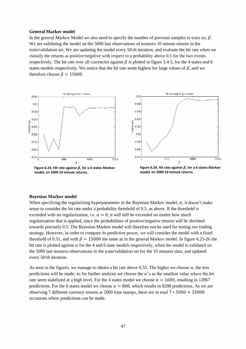
47

General Markov model

In the general Markov Model we also need to specify the number of previous samples to train on, .

We are validating the model on the 5000 last observations of nonzero 10 minute returns in the

train/validation set. We are updating the model every 50:th iteration, and evaluate the hit rate when we

classify the returns as positive/negative with respect to a probability above 0.5 for the two events

respectively. The hit rate over all currencies against is plotted in figure 3.4-5, for the 4 states and 6

states models respectively. We notice that the hit rate seem highest for large values of , and we

therefore choose .

Bayesian Markov model

When specifying the regularizing hyperparameter in the Bayesian Markov model, , it doesn’t make

sense to consider the hit rate under a probability threshold of 0.5, as above. If the threshold is

exceeded with no regularization, i.e. , it will still be exceeded no matter how much

regularization that is applied, since the probabilities of positive/negative returns will be shrinked

towards precisely 0.5. The Bayesian Markov model will therefore not be used for testing our trading

strategy. However, in order to compare its predictive power, we will consider the model with a fixed

threshold of 0.51, and with the same as in the general Markov model. In figure 6.25-26 the

hit rate is plotted against for the 4 and 6 state models respectively, when the model is validated on

the 5000 last nonzero observations in the train/validation set for the 10 minutes data, and updated

every 50:th iteration.

As seen in the figures, we manage to obtain a hit rate above 0.55. The higher we choose , the less

predictions will be made, so for further analysis we choose the ’s as the smallest value where the hit

rate seem stabilized at a high level. For the 4 states model we choose , resulting in 12867

predictions. For the 6 states model we choose , which results in 8298 predictions. As we are

observing 7 different currency returns at 5000 time stamps, there are in total

occasions where predictions can be made.

Figure 6.23. Hit rate against , for a 4 states Markov model, on 5000 10 minute returns.

Figure 6.24. Hit rate against , for a 6 states Markov model, on 5000 10 minute returns.

48

Figure 6.25. Hit rate against for a 4 states Bayesian Markov model, on 5000 10 minute returns.

Figure 6.25. Hit rate against for a 6 states Bayesian Markov model, on 5000 10 minute returns.

49

7. Results

The results will be presented as the performances on the test sets defined in 6.1. For the 10 minute data

we validate the models on the 10 000 latest observations in the test set, and for the weekly data on the

whole test set i.e. 280 observations. In section 7.1 we will investigate the predictive power of the

models using the RMSE and the hit rate as performance measures. In section 7.2 we will investigate

the performance of our trading strategies using the Sharpe ratio as performance measure.

7.1 Results of predictive power

When considering the hit rates of classified positive/negative returns, it is crucial to investigate the

percentage of positive/negative returns in the whole data samples. These numbers are presented for all

currencies respectively, for the 10 minute data in table 7.1 and for the weekly data in table 7.2. We are

not counting the zero returns, since these are not taken into account when computing the hit rates.

As seen in table 7.1, the percentage of positive/negative returns in the 10 minute data seem very

concentrated around 50%, and we therefore believe that significant results above 50% in this case do

indicate predictive power in our models.

In table 7.2 for the weekly data, the percentages differs quite a lot from 50% for some currencies. For

example 55% of the returns of the Swedish krona are positive. One should keep this in mind when

judging the resulting hit rates.

Table 7.1 Percentages of positive/negative returns, for all currencies on the whole data set of nonzero 10 minute

returns (38 000 observations).

Currency Percentage of positive returns Percentage of negative

returns

AUD 50.32% 49.68%

CAD 49.74% 50.26%

CHF 49.99% 50.01%

EUR 50.36% 49.64%

GBP 50.1% 49.9%

JPY 49.68% 50.32%

NZD 50.31% 49.69%

Total 50.07% 49.93%

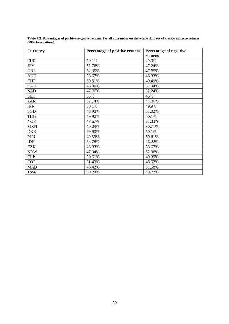
50

Table 7.2. Percentages of positive/negative returns, for all currencies on the whole data set of weekly nonzero returns

(980 observations).

Currency Percentage of positive returns Percentage of negative

returns

EUR 50.1% 49.9%

JPY 52.76% 47.24%

GBP 52.35% 47.65%

AUD 53.67% 46.33%

CHF 50.51% 49.49%

CAD 48.06% 51.94%

NZD 47.76% 52.24%

SEK 55% 45%

ZAR 52.14% 47.86%

INR 50.1% 49.9%

SGD 48.98% 51.02%

THB 49.90% 50.1%

NOK 48.67% 51.33%

MXN 49.29% 50.71%

DKK 49.90% 50.1%

PLN 49.39% 50.61%

IDR 53.78% 46.22%

CZK 46.33% 53.67%

KRW 47.04% 52.96%

CLP 50.61% 49.39%

COP 51.43% 48.57%

MAD 48.42% 51.58%

Total 50.28% 49.72%

51

General VAR

In table 7.3 the RMSE for the general VAR1 model divided by the RMSE for a random walk model

(when all returns are predicted zero) and the hit rates (where positive predicted values above zero

corresponds to predictions of positive returns and vice versa), for all currencies, are presented for the

10 minutes data. Notice that all currencies are predicted worse using the VAR model compared to the

random walk, with respect to the RMSE. However, some currencies seem to have hit rates

significantly greater than 0.5 at the 1% level.

In table 7.4 the RMSE for the general VAR1 model divided by the RMSE for a random walk model

and the hit rates, for all currencies, are presented for the weekly data. Note that all currencies are

predicted worse compared to the random walk, some with more than the double RMSE. However, the

total hit rate is significantly above 0.5 at the 10% level.

Table 7.3. RMSE for the VAR1 model divided by the RMSE for a random walk model, and the hit rate when

validating the model on 10 000 observations of 10 minute returns. *** denotes a hit rate significantly larger than 0.5 at

the 1% level.

Currency Hit rate

AUD CAD CHF EUR GBP JPY NZD Total

Table 7.4. RMSE for the VAR1 model divided by the RMSE for a random walk model, and the hit rate when

validating the model on 280 observations of weekly returns. ***, ** and * denotes a hit rate significantly larger than

0.5 at the 1%, 5% and 10% level respectively.

Currency Hit rate

EUR JPY GBP AUD CHF CAD NZD SEK ZAR INR SGD THB NOK MXN DKK PLN IDR

52

CZK KRW CLP COP MAD Total

Bayesian VAR

10 minute returns

In tables 7.5-7 the RMSE for the Bayesian VAR models divided by the RMSE for a random walk

model and the hit rates, for all currencies, are presented for the 10 minutes data. Notice that all

currencies get a higher RMSE with our model compared to the random walk model. However, the

total hit rate for the VAR1 model is significantly greater than 0.5 at the 1% level, which indicates that

the model has a little predictive power.

Table 7.5. RMSE for the VAR1 model divided by the RMSE for a random walk model, and the hit rate when

validating the model on 10 000 observations of 10 minute returns. *** denotes a hit rate significantly larger than 0.5 at

the 1% level.

Currency Hit rate

AUD CAD CHF EUR GBP JPY NZD Total

53

Table 7.6. RMSE for the VARX1 model divided by the RMSE for a random walk model, and the hit rate when

validating the model on 10 000 observations of 10 minute returns. *** denotes a hit rate significantly larger than 0.5 at

the 1% level.

Currency Hit rate

AUD CAD CHF EUR GBP JPY NZD Total

Table 7.7. RMSE for the VAR4 model divided by the RMSE for a random walk model, and the hit rate when

validating the model on 10 000 observations of 10 minute returns. ** and * denotes a hit rate significantly larger than

0.5 at the 5% and 10% level respectively.

Currency Hit rate

AUD CAD CHF EUR GBP JPY NZD Total

54

Weekly returns

In tables 7.8-9 the RMSE for the Bayesian VAR models divided by the RMSE for a random walk

model and the hit rates, for all currencies, are presented for the weekly data. The VAR1 model

performs slightly better than the random walk for most currencies, and gets a bit smaller total RMSE

(only 0.04%). Best predicted is the Thai Baht with more than 1% lower RMSE than the random walk,

and a hit rate of 0.5964. The VAR4 model does not perform well at all, with a total hit rate below 0.5.

Table 7.8. RMSE for the VAR1 model divided by the RMSE for a random walk model, and the hit rate when

validating the model on 280 observations of weekly returns. *** and ** denotes a hit rate significantly larger than 0.5

at the 1% and 5% level respectively.

Currency Hit rate

EUR JPY GBP AUD CHF CAD NZD SEK ZAR INR SGD THB NOK MXN DKK PLN IDR CZK KRW CLP COP MAD Total

55

Table 7.9. RMSE for the VAR4 model divided by the RMSE for a random walk model, and the hit rate when

validating the model on 280 observations of weekly returns. *** denotes a hit rate significantly larger than 0.5 at the

1% level.

Currency Hit rate

EUR JPY GBP AUD CHF CAD NZD SEK ZAR INR SGD THB NOK MXN DKK PLN IDR CZK KRW CLP COP MAD Total

General Markov

In tables 7.10-11 the hit rates (with a threshold of 0.5 on the transition probabilities) are presented for

the 10 minute returns using a Markov model of 4 and 6 states respectively. All hit rates are

significantly greater than 0.5 at the 1% level for both models, which strongly indicates that the models

have predictive power.

Table 7.10. Hit rates for the 4 states Markov model when validating the model on 10 000 observations of 10 minute

returns. *** denotes a hit rate significantly larger than 0.5 at the 1% level.

Currency Hit rate

AUD CAD CHF EUR GBP JPY NZD Total

56

Table 7.11. Hit rates for the 6 states Markov model when validating the model on 10 000 observations of 10 minute

returns. *** denotes a hit rate significantly larger than 0.5 at the 1% level.

Currency Hit rate

AUD CAD CHF EUR GBP JPY NZD Total

Bayesian Markov

In tables 7.12-13 the hit rates are presented for the 10 minute returns using the Bayesian Markov

model of 4 and 6 states respectively, with a threshold of 0.51 on the transition probabilities. Note that

for the 6 states model all hit rates are greater than for the general Markov models, which indicates that

we can increase the predictive power by shrinking the transition probabilities. This can be useful when

one only wants to trade at certain times, e.g. for reducing the transaction costs, but these strategies will

not be further discussed in this thesis.

Table 7.12. Hit rates for the 4 states Bayesian Markov model when validating the model on 10 000 observations of 10

minute returns. *** denotes a hit rate significantly larger than 0.5 at the 1% level.

Currency Hit rate

AUD CAD CHF EUR GBP JPY NZD Total

Table 7.13. Hit rates for the 6 states Bayesian Markov model when validating the model on 10 000 observations of 10

minute returns. *** denotes a hit rate significantly larger than 0.5 at the 1% level.

Currency Hit rate

AUD CAD CHF EUR GBP JPY NZD Total

57

7.2 Results of trading performance

To investigate whether it is possible to make any profit using our models, we validate our performance

with respect to the Sharpe ratios using the trading strategies described in 4.1. The portfolio returns are

computed by the formula (also given in 4.1):

∑

∑| |

Notice that the parameter , denoting the transaction costs, will be given in terms of daily standard

deviations for the weekly data and standard deviations on 10 minutes for the 10 minute data.

First we will compare the different model performances when no transaction costs are taken into

account. Then, we will investigate what transaction costs that can be allowed while still making profit,

when using the best performing models for weekly and 10 minute returns respectively.

Without transaction costs

In tables 7.14-15 the Sharpe ratios for the models are presented for 10 minute and weekly returns

respectively, when not taking any transaction costs into account. In table 7.14 we notice that all Sharpe

ratios are positive for 10 minute returns, and that the Markov models dominate the others by far with

Sharpe ratios above 9. This was expected since the Markov models dominated the others also with

respect to the hit rates.

In table 7.15, for the weekly returns, we notice that the only model that produces a positive Sharpe

ratio is the Bayesian VAR1 model, which also was the one that produced the best prediction results

with respect to the RMSE.

Table 7.14. Sharpe ratios for the different models for 10 minute returns. Validated on 10 000 samples of 10 minute

returns.

Model Sharpe ratio

General VAR1 Bayesian VAR1 Bayesian VARX1 Bayesian VAR4 Markov, 4 states Markov, 6 states

Table 7.15. Sharpe ratios for the different models for weekly returns. Validated on 280 samples of weekly returns.

Model Sharpe ratio

General VAR1 Bayesian VAR1 Bayesian VAR4

58

The total yields in terms of daily and 10 minute standard deviations for the best performing models on

10 minutes and weekly returns, i.e. the 4 states Markov model and the Bayesian VAR1 model, are

plotted in figures 7.1-2. No transaction costs are taken into account. While the Markov model for 10

minute returns seem to perform well constantly over time, the Bayesian VAR1 model for weekly

returns seem to underperform during 2009 and 2010, but thereafter perform very well.

Figure 7.1. Total yield over time for the 4 states Markov model for 10 minute returns, when no transaction costs are taken into account. The model is validated on 10 000 observations of 10 minute returns.

Figure 7.2. Total yield over time for the Bayesian VAR1 model for weekly returns, when no transaction costs are taken into account. The model is validated on 280 observations of weekly returns.

59

With transaction costs

In figure 7.3 the Sharpe ratio against the average transaction cost is plotted for the 10 minute returns

using the best performing model, i.e. the 4 states Markov model. Notice that the Sharpe ratio becomes

negative with average transaction costs of 0.021 standard deviations on 10 minutes, or about

√

daily standard deviations.

In figure 7.4 the Sharpe ratio is plotted against the average transaction cost for the weekly returns,

using the Bayesian VAR1 model (which performed best without transaction costs). The Sharpe ratio is

positive for transaction costs below 0.0415 daily standard deviations, considerably larger than for the

10 minutes data. It should however be noted that the 10 minute data is measured as arithmetic returns,

whilst the weekly data are logarithmic returns. One can approximate the resulting normalized

quantities of arithmetic and geometric returns as the same, resulting in approximately the same

transaction costs measured in standard deviations.

The transaction costs involved varies in time and between market participants, depending on the

spread between bid and ask prices, what amounts that are traded and what brokerage fee that is

offered. However, it can be considered hard to get as low transaction costs as needed for the Sharpe

ratio to be positive when trading at a 10 minute horizon, i.e. 0.0034 daily standard deviations, while it

should be very possible to get lower transaction costs than 0.0415 daily standard deviations, as needed

for the weekly trading horizon.

Figure 7.3. Sharpe ratio for the 10 minute returns against transaction costs in terms of standard deviations on 10 minutes, for the 4 states Markov model validated on a sample of 10 000 observations.

Figure 7.4. Sharpe ratio for the weekly returns against transaction costs in terms of daily standard deviations, for the Bayesian VAR1 model validated on a sample of 280 weekly observations.

60

8. Conclusions

An aim of this thesis was to find models that could systematically predict future returns of foreign

exchange rates better than a random walk model. This is something that has been achieved, with high

significance for the 10 minute returns.

Another aim was to find a strategy that, by making use of the forecasting models, can yield a profit.

This highly depends on the transaction costs involved, but we have shown that a positive Sharpe ratio

had been achieved using the Bayesian VAR1 model for weekly returns out of sample, even for

moderately high transaction costs.

8.1 The 10 minute horizon

For data sampled on 10 minutes, we found that a Markov model can predict whether the return on the

next 10 minutes interval will be positive or negative accurately in significantly more than 50% of the

cases, and that the predictive power seemed to increase even more with a regularized Bayesian

Markov model. This indeed means that the random walk model can be rejected.

However, there might be an intuitive explanation of the positive prediction results, which would ruin

the possibility of making profits using this model. Even if the foreign exchange market is very liquid,

there will always be a spread between the bid and ask prices. If a market participant choose to cross

the spread, i.e. buy at the ask price or sell at the bid price, the latest noted price will temporarily be

higher/lower, and thereafter decrease/increase to somewhere in the middle of the spread. This might

explain the negative autocorrelation at lag 1 for the 10 minute returns, and would imply that one

cannot expect to be able to trade at the same price as the latest noted and thereby that this pattern

cannot be taken into advantage for making profits.

Another aspect is the transaction costs. The simple trading strategy investigated, where one is trading

on every 10 minute interval and updating the portfolio weights totally based on the prediction of the

return on the next 10 minute interval, has shown to be very successful with a Sharpe ratio above 9 out

of sample if no transaction costs are taken into account. However, the Sharpe ratio becomes negative

even when very small transaction costs are considered. The dramatic negative effect of the transaction

costs depends a lot on the fact that the portfolio weights change drastically on every 10 minute interval

with the strategy considered. However, there are ways to reduce the variability of the weights, and

thereby reduce the transaction costs. This is indeed something that would be interesting to investigate

in future research.

8.2 The weekly horizon

The Bayesian VAR1 model for weekly returns performed slightly better than the random walk model

out of sample with respect to the RMSE, and the hit rates were shown to be significantly above 50%

for two currencies, the Thai Baht (at the 1% level) and the South Korean Won (at the 5% level). This

indicates that the random walk hypothesis can be rejected, even if the arguments are somewhat vaguer

than in the case of 10 minute returns. It was also shown that the RMSE can be decreased a lot using a

Bayesian model compared to the frequentist approach.

For the weekly returns we made the assumption of causality, after adding non-causally sampled daily

returns together at a weekly basis. One should keep this in mind, even if it is quite intuitive to assume

that a few hours of knowledge about one currency not influences the future weekly return of another

currency.

61

The trading strategy suggested yields a positive Sharpe ratio out of sample, even when moderately

high transaction costs are considered. If one only had considered the period past 2011, the Sharpe ratio

would be even higher, and it is very interesting to have found a trading strategy which actually had

performed well out of sample in very recent times.

62

9. Bibliography

Bank For International Settlements. (2013, September 5). Triennial Central Bank Survey of foreign

exchange turnover in April 2013. Retrieved June 04, 2014, from www.bis.org:

http://www.bis.org/press/p130905.htm

Baviera, R., Vergni, D., & Vulpiani, A. (2000). Markovian approximation in foreign exchange markets.

Physica A 280, 566-581.

Bennet, C., & Gil, M. A. (2012). Measuring Historical Volatility. Santander Investment Bolsa.

Bowman, A. W., & Azzalini, A. (1997). Applied Smoothing Techniques for Data Analysis. Oxford

Science Publications.

Carriero, A., Kapetanios, G., & Marcellino, M. (2008). Forecasting Exchange Rates with a Large

Bayesian VAR. European University Institute.

Fama, E. (1965). The Behavior of Stock-Market Prices. The Journal of Business Vol. 38, No.1, 34-105.

Karlsson, S. (2012). Forecasting with Bayesian Vector Autoregressions. Örebro University.

Litterman, R. B. (1979). Techniques of forecasting using vector autoregressions. Federal Reserve Bank

of Minneapolis.

Lo, A. W., & MacKinlay, A. C. (1999). A Non-Random Walk Down Wall Street. Princeton University

Press.

Malkiel, B. (1973). A Random Walk Down Wall Street. W. W. Norton & Company Inc.

Meese, R. A., & Rogoff, K. (1983). Empirical Exchange Rate Models of the Seventies. Journal of

International Economics 14, 3-24.

Powell, J. L. (2008). Notes On Nonparametric Regression Estimation. Retrieved June 4, 2014, from

University of California, Berkeley: http://eml.berkeley.edu/~powell/e241a_sp06/nrnotes.pdf

Robert, C. P. (2001). The Bayesian Choice, 2nd Ed. Springer.

Wikipedia, AIC. (2014, May 20). Akaike information criterion. Retrieved June 6, 2014, from

www.wikipedia.org: http://en.wikipedia.org/wiki/Akaike_information_criterion

Wikipedia, BIC. (2014, April 9). Bayesian information criterion. Retrieved June 4, 2014, from

www.wikipedia.org: http://en.wikipedia.org/wiki/Bayesian_information_criterion

Wikipedia, MPT. (2014, June 2). Modern portfolio theory. Retrieved June 4, 2014, from

www.wikipedia.org: http://en.wikipedia.org/wiki/Modern_portfolio_theory