fundamental limits on synchronizing clocks over...
TRANSCRIPT

1
Fundamental limits on synchronizing clocks overnetworks
Nikolaos M. Freris, Member, IEEE, Scott R. Graham, Member, IEEE, and P. R. Kumar, Fellow, IEEE
Abstract—We present fundamental impossibility results onclock synchronization in wireline or wireless networks, andsharply characterize what is feasible. We consider a networkof n nodes with affine clocks, with one node designated asa reference. Each other node’s clock is described by a skew(relative speedup with respect to the reference clock), and anoffset at time 0 (say) with respect to the reference clock. Inorder to establish impossibility results, we allow for noiselesscommunication of an unlimited number of messages, that maycontain any information that the transmitting node knows aboutor from current or past packets that it has sent or received. Thesynchronization problem consists of determining all the unknownparameters, skews and offsets of all the clocks, as well as thedelays of all the communication links. All unknown parametersare assumed to be time-invariant but unknown. The assumptionsof time-invariant parameters and unlimited exchange of noiselesstime-stamps consider the most idealistic scenario and are madefor analyzing the feasibility of the problem, and thus sharplydelineating impossibility results. This is because if somethingis infeasible under these ideal assumptions, it would also beinfeasible in more realistic noisy scenarios.
We prove that determining all unknown parameters is impos-sible. We show that all nodal skews, as well as all round-tripdelays between every pair of nodes, can be determined correctly.However, the vector of unknown link delays and clock offsetscan only be determined up to an (n− 1)-dimensional subspace.Each degree of freedom in this subspace corresponds exactly tothe offset of one of the (n−1) clocks with respect to the referenceclock. On the positive side, we show that every transmitting nodecan predict precisely the time indicated by the receiver’s clockat the instant it receives the packet.
If we further invoke causality, that packets cannot be receivedbefore they are transmitted, the uncertainty set can be reducedto a polyhedron in Rn−1. We provide necessary and sufficientconditions on the network topology for the polyhedron to becompact and have a non-empty interior.
We further study the problem of receiver-receiver synchro-nization, where only receipt times are available, but no time-stamping is done by the sender. We show that all nodal skewscan still be determined correctly, but delay differences betweenneighboring communication links with a common sender canonly be characterized up to an affine transformation of the(n − 1) unknown offsets. Moreover, causality does not help;the uncertainty set remains as a translate of Rn−1.
We also investigate structured models for link delays asthe sum of a transmitter-dependent delay, a receiver-dependentdelay, and a propagation delay, where the latter is known,e.g., via GPS position information. We identify conditions onthe transmission and reception delays which permit a uniquesolution, and conditions under which the number of the residual
Nikolaos M. Freris and P. R. Kumar are with the Dept. of ECEand CSL, University of Illinois at Urbana-Champaign, 1308 W. MainStreet, Urbana, IL 61801, USA. Email: [email protected],[email protected].
Major Scott R. Graham is with Air Force Institute of Technology, USA.Email: [email protected].
Please address all correspondence to the third author [email protected].
degrees of freedom is a constant independent of network size.
Index Terms—Clock Synchronization, Networked Control,Sensor Networks, Scheduling, Clock Skews, Clock Offsets, De-lays.
I. INTRODUCTION
Distributed clocks generally don’t agree. Yet, several appli-cations in sensor networks and networked control are groundedin accurate clock synchronization. Applications in networkedcontrol include closing control loops or coordinating events ina decentralized system, such as a traffic control or collisionavoidance system. In sensor networks, clock synchronizationrequirements are omnipresent; in tracking, target localization,data fusion, and power-efficient duty-cycling. Scheduled op-erations in wireless networks, e.g., slotted protocols, alsorequire accurate clock synchronization. This motivates thestudy of clock synchronization over communication networks.As we head towards the era of event-cum-time driven systemsfeaturing the convergence of computation and communicationwith control, the need for well-synchronized clocks becomesincreasingly important, affecting system performance, QoSand safety.
A. Notions of network clock synchronization
There are three main degrees of clock synchronizationthat may be required by the specifications of a particularapplication.
1) Ordering of events. In this case, the problem is to createa right chronology of the events in the entire network.For this purpose, knowledge of the exact time instantsis not required, yet an ordering of events that occur atdifferent nodes or the same node has to be determined.This is the weakest notion of synchronization but issufficient for many applications such as financial trans-actions involving locks in databases, several monitoringapplications, etc. This problem was first thoroughlystudied in [3] where the notion of virtual clocks wasfirst introduced.
2) Relative Synchronization. Here, the goal of synchroniza-tion is to estimate the relative drift among a set of clocksin the network. This information can be then used totranslate time-stamps from one clock to the units of anyother clock. This has the advantage that the translationmechanism does not create undesirable dependencies byresetting clocks in hosts [2], [16], and gives rise to thenotion of relative clocks.
3) Absolute Synchronization. This is the strongest notion ofclock synchronization in a network. Each node has an

2
absolute clock and the goal is to set all clock displays toagreement, so that a global definition of time is achievedin the entire network. Networked control applicationstypically require this stronger type of synchronization.
From the above definitions it is immediate that absolutesynchronization implies relative synchronization which in turnimplies ordering of events in a network. However, if we definea particular node as reference, then relative synchronizationcan be used to achieve absolute synchronization.
In this paper we focus on relative and absolute synchroniza-tion.
B. Problem under study
The specific problem that we address is the characterizationof the extent to which clock synchronization is even feasible.We consider clocks which run at a constant, but not necessarilyidentical speed. Each clock is characterized by its “skew,” i.e.,relative speed with respect to a reference clock, as well as an“offset,” i.e., the time difference from the reference clock ata particular time, which, for convenience, we take to be thetime 0 of the reference clock. Thus, we consider affine clocks.
Our purpose is to exhibit fundamental impossibility resultsin clock synchronization. For this purpose, we will considerthe ideal scenario where neither offset nor skew drifts withtime and all time-stamps are noiseless. Clearly, if clockscannot be synchronized in such an ideal environment, thenthey cannot be synchronized in the presence of noise. For thesame reason, we suppose that packets suffer delays dependenton the transmitter-receiver communication pair. We allow fornoiseless communication where latencies in packet transferare deterministic and time-invariant but unknown. In the samespirit, we will allow nodes to exchange an arbitrary numberof packets containing any information that the transmittingnode knows about current or past packets that the node hassent, or any information contained in past packets that it hasreceived. This includes the time that the current packet is beingsent according to the transmitter’s clock, as well as the timesthat it received previous packets. This also includes hearsayinformation that another node may send to it concerninginformation that it received from yet other nodes. Thus weallow for packets to contain any causally acquired informationthat the sender may have.
C. Characterization of limits on clock synchronization
We show that while all skews can be perfectly determined,the delays of the links and the offsets of the nodes cannot beexactly determined. Specifically, the vector of all link delaysand node offsets can only be characterized up to a translationof an (n − 1)-dimensional subspace, where n is the numberof nodes. In fact, we show that these (n− 1) indeterminableparameters can be regarded as estimates of the nodal offsets.
If we further invoke causality, i.e., that packets cannot bereceived before they are sent, then the uncertainty regionis a polyhedron that is explicitly characterized. We providenecessary and sufficient conditions on the network topologyfor the polyhedron to be compact and have a non-emptyinterior.
We also study the problem of receiver-receiver synchroniza-tion where nodes only exchange information on the times atwhich they receive broadcast packets, without any sender time-stamping. We show that nodal skews can still be determinedcorrectly, but only delay differences between neighboring com-munication links with a common sender, and not actual delaysthemselves, can be expressed affinely by (n − 1) unknownoffsets. We prove that causality cannot be exploited and thatthe uncertainty set remains the entire space Rn−1. Moreover,round-trip delays cannot be estimated from the known data.
We further study the case where link delays have the struc-ture of being the sum of a transmitter-specific delay, a receiver-specific delay, and a known electromagnetic propagation delay.For such cases, we again characterize the uncertainty set.
The rest of the paper is organized as follows. In Section IIwe summarize related literature on clock synchronization. InSection III, we introduce the affine model for the clocks, andthe assumptions on the delays. In Section IV, we formulatethe problem , provide a formal description of the inter-nodecommunication, present an impossibility result for the caseof two clocks [2], and describe the structure of the residualuncertainty. In Section V, we describe the network clocksynchronization problem and provide necessary and sufficientconditions on the network topology for the determination ofall nodal skews. In Section VI, we prove that with no furtherassumption on the unknown delays, determining the offsetsis impossible for any network topology under any commu-nication scheme. We show that while skews can be reliablydetermined from known data, offsets involve an inherent inde-terminacy. Furthermore, we outline a method for the optimalselection of the offset vector. In Section VII, we study theproblem of receiver-receiver synchronization in a network, andprove the infeasibility and the fundamental fact that causalitycannot be exploited in this case. In Section VIII, we studythe problem when the delays have an additive decompositionin terms of transmission, reception and propagation latencies.Finally, in Section IX, we cite some concluding remarks ofour work.
II. RELATED LITERATURE
In distributed systems, ordering of events is crucial for manyapplications. Lamport [3] shows how to causally order eventsby defining the notion of virtual clocks.
In [13] the authors study the problem of synchronizingclocks in a fully connected network and show that an uncer-tainty of ε in packet delivery leads to a maximum synchroniza-tion error no less than ε(1− 1
n ). In [12] the authors derive apolyhedral uncertainty set for link delays in a general networktopology. Establishing the impossibility of determining theoffset in pairwise clock synchronization was carried out in[2], [16]. A similar result is noted in [14], though withouta complete rank-based proof. The main result is that whiledetermining the relative skew between two clocks is possible,it is impossible to do so for offsets, unless delays in thetwo-way communication are assumed to be symmetric. Theproof of this result together with an extended analysis of theuncertainty set for the problem is presented in Section IV andis used to establish the results for the network case.
3
The basic mechanism for synchronizing clocks is to ex-change time-stamped packets, or “pings,” between nodes. TheNetwork Time Protocol (NTP [7]) is a widely used hierarchicalprotocol implemented to achieve absolute synchronization ofclocks in large networks like the Internet. NTP providesaccuracy in the order of milliseconds [7] by typically usingGPS to achieve synchronization to external sources that areorganized in levels called stratums. While this accuracy maybe sufficient for some applications, recent applications inwireless sensor networks typically require precision in theorder of microseconds (µs). Moreover, in some cases, e.g.,indoors, or during solar flares, GPS may be unavailable.
In sensor networks and networked control, a variety of al-gorithms have been suggested for synchronization such as theReference Broadcast Synchronization (RBS [8]) and FloodingTime Synchronization Protocol (FTSP [9]). RBS is a receiver-receiver synchronization algorithm, which uses the broadcastnature of the wireless medium. It does not make use of senderside time-stamping. Nodes broadcast packets and the nodesthat receive the transmission then record and exchange thereception times so as to estimate the receiving nodes’ clockdifferences. The scheme attains precision within 11 µs. InFTSP [9], the Medium Access Control (MAC) time-stampingcapabilities are exploited and linear regression is used tocompensate for clock drifts; the precision is of the order of10 µs for absolute synchronization in a network with severalhundreds of nodes. Elson, Karp, Papadimitriou and Shenker[6] have studied fundamental properties of minimum varianceestimates, and presented algorithms. Solis, Borkar and Kumar[4] have developed and implemented a decentralized asyn-chronous algorithm based on spatial smoothing, and performedcomparative evaluations showing improvements. Giridhar andKumar [5] have analyzed the performance of this spatialsmoothing method, both to determine asymptotic accuracyas well as convergence rates. In [15] the authors studied astochastic differential equation model-based approach to clocksynchronization.
III. MODEL FOR CLOCKS AND DELAYS
A. Affine model for clocks
Throughout this paper, we will assume the simple model ofaffine clocks. Denoting the time of a fixed reference clock byt, we will assume that the display of a clock j in the networkat time t, denoted by τj(t), satisfies
τj(t) := ajt+ bj . (1)
We call the ratio of the speeds of the two clocks, aj , as theskew1, while the difference in their displays will be referred toas the offset at a particular instant. Above, bj is the offset ofclock j at the time 0 of the reference clock. An affine clockcan thus be represented by the pair of parameters (aj , bj). Forthe purpose of establishing fundamental impossibility results,unknown parameters such as (aj , bj) are considered to beconstant time-invariant parameters, throughout the entirety ofthis paper. The reason for such an assumption is that if we can
1Some authors [14] define the skew to be aj − 1 but here we use theterminology of [2].
prove that the determination of the unknown parameters is im-possible under this idealistic scenario, then impossibility willnaturally carry over to the case of time-varying parameters.
We also suppose that aj > 0, i.e., forward evolution ofthe time in all clocks. In practice, the skew takes values veryclose to 1.2 On the contrary, offsets are sign-indefinite and sono constraints are imposed on the values of bj .
For notational convenience, we fix node 1’s clock to be thereference clock; hence a1 := 1, b1 := 0. A useful formula thatprovides time translation of clock j’s time to clock i’s timeunits, as can be obtained from (1), is
T ji (τj) :=aiajτj + bi −
aiajbj . (2)
The reason for assuming such clock model is because thisis the simplest model that captures the reality that clocks arenot synchronized because of non-nominal speeds and offsets.The model assumes constant but unknown clock skew and hasbeen validated to be accurate for some clocks [11], [17], [18].Establishing impossibility of clock synchronization under theaffine model implies impossibility for more general modelsthat capture skew variations, even though the uncertainty setsderived in this paper do not apply in such cases. A stochasticmodel for clocks and delays was introduced in [15].
B. Model for packet delay
Delays in packet delivery constitute a fundamental limi-tation in synchronizing clocks over wireless networks sincethey can be much larger than the required synchronizationprecision. We will suppose that whenever a packet is sent bynode i, it is received by node j after a delay of dij time units(measured in the time units of the reference clock, clock 1).The delays {dij} are assumed to be unknown but fixed; this isagain an ideal scenario used to establish general impossibilityresults.
By the word “delay” here, we mean not only the electro-magnetic propagation delay, but rather the sum of all delaysincurred by a packet after it is time-stamped by the transmitterand before it is time-stamped by the receiver, as discussedin Section VIII. With the exclusion of the electromagneticpropagation delay, the other delays can depend on the commu-nication and computation platforms of the nodes involved andthe load experienced at them. Due to this heterogeneity, delayscannot be expected to be symmetric or identical between links.Hence we allow dij 6= dji and dij 6= dik.
Even though the link delays are not clock parameters, theirestimation is, however, a very important bi-product of clocksynchronization, since knowledge of such quantities is crucialfor many applications including routing, and the stability ofnetworked control loops [2], [16].
IV. PAIRWISE SYNCHRONIZATION OF TWO CLOCKS
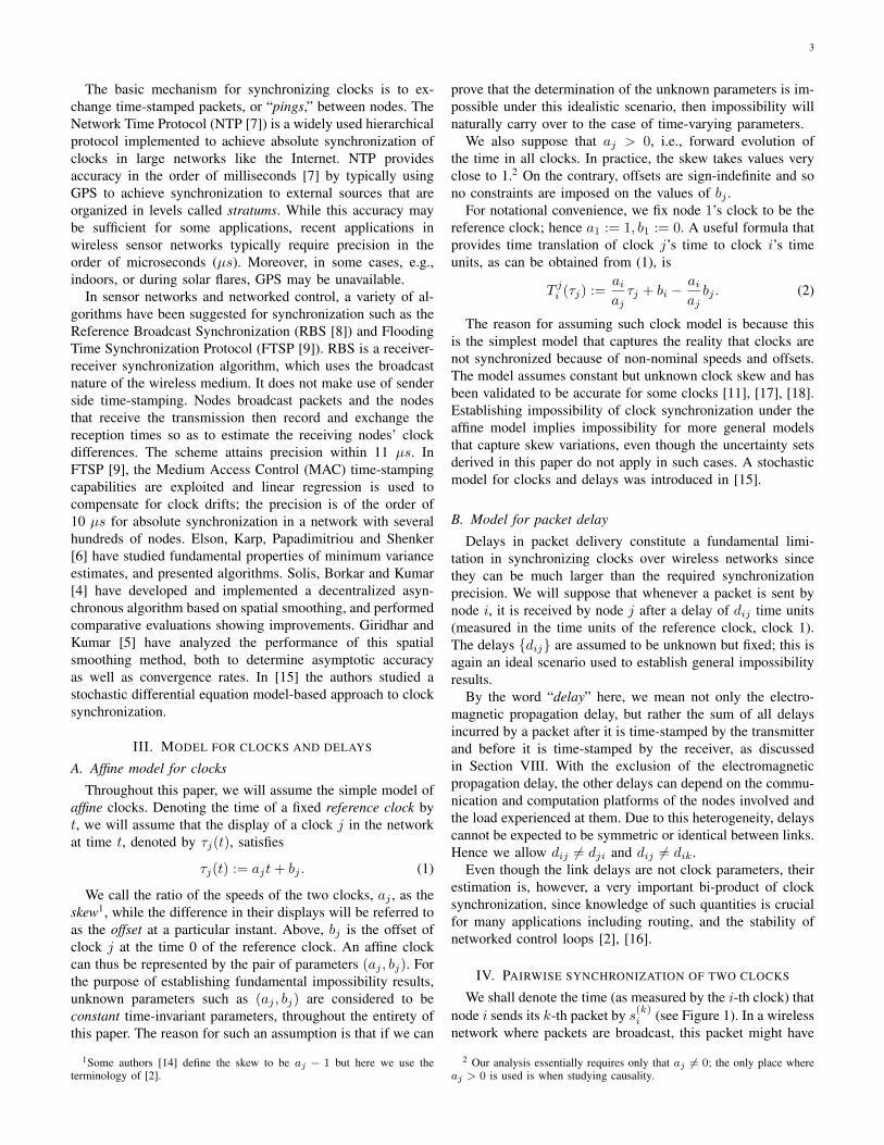
We shall denote the time (as measured by the i-th clock) thatnode i sends its k-th packet by s(k)
i (see Figure 1). In a wirelessnetwork where packets are broadcast, this packet might have
2 Our analysis essentially requires only that aj 6= 0; the only place whereaj > 0 is used is when studying causality.

4
τj(t)
τi(t)
r(1)i,j s
(1)j
r(1)j,is
(1)i
r(2)i,j s
(2)j
T ji (r
(1)i,j ) T j
i (s(1)j )
dij dji
t
Node j
Node i
Node 1
dij dji
r(2)j,is
(2)i T j
i (r(2)i,j ) T j
i (s(2)j )
Fig. 1. Message exchanges between two nodes
multiple receivers, so we avoid specifying the receiver in theabove notation. We will denote by r(k)
i,j the time (as measuredby the j-th clock) that node j receives the k-th packet sent bynode i (see Figure 1)3.
In this section we will consider the case of only two nodestrying to synchronize their clocks. Thus, suppose that clock1 (the reference) and clock j are the only two clocks in thesystem. As shown in Figure 1 (in this case i = 1), the twonodes are allowed to communicate repeatedly by exchangingtime-stamped packets. In the k-th packet sent by node 1, thetransmitting node includes its current transmission time-stamp,s
(k)1 , as measured by its clock just before the transmission.
Upon receiving this packet, the receiving node j records thetime (according to its local clock) just after it receives thepacket, r(k)
1,j . Similarly, when node j is transmitting, we assumethat the time-stamps s(k)
j , r(k)j,1 are available. Recall that all
time measurements are assumed noiseless, since showing inde-terminacy of the parameters even for noiseless measurementswould imply such indeterminacy for noisy models, too.
We allow for every packet to contain information about allthe past receipt times of all prior packets as recorded at thatnode, so that each node contains a full log of the transmit-ting/receiving times of packets between them. Equivalently,we can suppose that there is a “genie” that has access to alltransmit and receipt times for all packets, as recorded by theirrespective clocks.
As shown in [2], [16], it is impossible to estimate all fourunknown parameters, (aj , bj , d1j , dj1), through any numberof packet exchanges, which is stated and proven next forcompleteness of presentation:
Theorem 1. (Impossibility of pairwise synchronization [2])Even under bilateral exchange of an infinite number of packetsbetween the two nodes j and 1, estimation of the entire four-tuple (aj , bj , d1j , dj1) is impossible.
Proof: Since a1 = 1, b1 = 0, the translation of node j’stime τj to the reference clock’s time t is given by
T j1 (τj) :=1
ajτj −
1
ajbj . (3)
For the k-th transmission of node 1 to node j, and vice-versa
3Note that the horizontal lines in Figure 1 represent time displays atdifferent clocks and are, in general, at different scales, since clocks may runat different speeds and also have an offset from one another.
we have (see also Figure 1):
1→ j : T j1 (r(k)1,j ) = s
(k)1 + d1j , (4)
r(k)1,j = ajT
j1 (r
(k)1,j ) + bj , (5)
j → 1 : r(k)j,1 = T j1 (s
(k)j ) + dj1, (6)
s(k)j = ajT
j1 (s
(k)j ) + bj . (7)
Substituting (4) into (5), and (6) into (7), we get
1→ j : r(k)1,j = ajs
(k)1 + ajd1j + bj , (8)
j → 1 : s(k)j = ajr
(k)j,1 − ajdj1 + bj . (9)
In order to obtain equations that are linear in unknowns, weconsider a nonlinear parametrization, (aj , ajd1j , ajdj1, bj), ofthe unknowns (aj , bj , d1j , dj1)
r(1)1,j
s(1)j
r(2)1,j
s(2)j...
=
s
(1)1 1 0 1
r(1)j,1 0 −1 1
s(2)1 1 0 1
r(2)j,1 0 −1 1...
......
...
ajajd1j
ajdj1bj
. (10)
Denoting the vector on the LHS above by y, the matrix on theRHS by A, and the vector on the RHS by x, we have y = Ax.We observe that y and A contain known information basedon the time-stamps, while x is the vector of the unknowns.
By the fact that the time-measurements are noiseless, weknow that for the measured (y,A) there exists a solution xto y = Ax, since the system of equations is consistent. Anecessary and sufficient condition for this solution to be uniqueis that the matrix A have full-rank, i.e., rank 4. This is also thenecessary and sufficient condition for the existence of a uniquesolution (aj , bj , d1j , dj1) to (10), since the parametrization(aj , bj , d1j , dj1) 7−→ x is bijective for aj 6= 0. However, thefourth column of A is the difference between the second andthe third column, and so A has rank at most 3.Remark 1.1 The first three columns of matrix A in (10) arelinearly independent if and only if either not all odd or notall even entries are the same, that is to say if there are atleast two distinct communication pings in one direction, andat least one ping in the other direction. In the sequel, we willassume, with no loss in generality that s(1)
1 < s(2)1 < · · · , and
s(1)j < s
(2)j < · · · , and restrict attention to the 4× 4 principal
submatrix of A, of rank 3, which yields the systemr
(1)1,j
s(1)j
r(2)1,j
s(2)j
=
s
(1)1 1 0 1
r(1)j,1 0 −1 1
s(2)1 1 0 1
r(2)j,1 0 −1 1
ajajd1j
ajdj1bj
. (11)
For convenience, we denote the finite linear system in (11) asy = Ax. The remaining pings contain no additional informa-tion not already contained in these four pings, for the purposeof determining the unknown parameters and estimating thedelays. Note also, that from (11), it suffices that a transmittedpacket contain information about its current transmit time andjust the transmit-receipt time-stamps of two past pings, one in
5
each direction4 since the receipt time of the packet will alsobe available to the receiver.
Since the above system does not admit a unique solution,we study the set of all solutions to (11). We will call this setof all solutions as the uncertainty set. It is the smallest setwithin which the true but unknown parameter vector can bedetermined to lie.
In the sequel, we use “ ˆ ” to denote any estimate ofunknown quantities, and “ * ” to refer to some specialquantities that can be derived from the data.
Theorem 2. (Characterization of the uncertainty set in pair-wise synchronization)
1) The skew can be precisely determined, even if there areonly two one-way pings, i.e., the link is unilateral 5.
2) The vector (bj , d1j , dj1)T of offset and delays can onlybe determined up to a translate of a one-dimensionalsubspace of R3. Each point in this one-dimensionaltranslated subspace corresponds to a particular estimateof the unknown offset.
3) The round-trip delay (d1j + dj1) can be determinedprecisely 6.
4) If we further use knowledge of causality, that packetscannot be received before they are sent, and also thataj > 0, then the uncertainty set for the offset reduces toan interval, whose length is proportional to the round-trip delay.
Proof: The null space of the matrix A in (11) is spannedby the vector (0,−1, 1, 1)T . Define (a∗j , d
∗1j , d
∗j1) by
a∗j :=r
(l)1,j − r
(k)1,j
s(l)1 − s
(k)1
=s
(l)j − s
(k)j
r(l)j,1 − r
(k)j,1
, (12)
a∗jd∗1j := r
(k)1,j − ajs
(k)1 , (13)
a∗jd∗j1 := ajr
(k)j,1 − s
(k)j . (14)
for k 6= l. Note that, since the first entry of the vector spanningthe null space is 0, we have that aj = a∗j , is the unique solutionfor the skew aj , i.e., the skew can be determined by a ratioof differences between received time-stamps and sent time-stamps. Then the vector (aj , bj , d1j , dj1)T fits the transmitand receive time-stamp data, i.e., x = (aj , aj d1j , aj dj1, bj)
T
satisfies y = Ax (and y = Ax), if and only ifaj
aj d1j
aj dj1bj
=
a∗j
a∗jd∗1j
a∗jd∗j1
0
+ bj
0−111
. (15)
Hence, aj = a∗j , bj ∈ R is arbitrary, and(d1j
dj1
)=
(d∗1jd∗j1
)+ bj
(− 1a∗j1a∗j
). (16)
4In fact, since A(i,j) is of rank 3, this system can be equivalentlyconstructed as a 3 × 4 system, by using only three distinct pings (two inone direction and one in the other), however we will use, with no loss ingenerality, a 4× 4 matrix for ease of presentation.
5This was also shown in [14].6This was also shown in [2],[12].
This proves 1), 2), and also 3) since
d1j + dj1 = d∗1j + d∗j1. (17)
For 4), we invoke causality, that is to say that packets cannotbe received before they are transmitted, which is equivalent toimposing the natural nonnegativity constraints on the delayestimates, d1j ≥ 0, dj1 ≥ 0. Since a∗j > 0, (16) immediatelyyields
bj ∈ [−a∗jd∗j1, a∗jd∗1j ]. (18)
hence the indeterminacy for the offset is a∗j (d∗j1 + d∗1j).
Remark 2.1 Note that determining the upper bound of theinterval in (18), requires only transmission from node 1 tonode j while determining the lower bound only needs node jto transmit to node 1.Remark 2.2 (Use of Lamport’s global ordering [3]). In ouranalysis of the consequence of causality, we have actuallyexploited all the available information provided by the globalordering described by Lamport in [3]. The ordering of eventsat a single node can be carried out trivially since all timeinstants are measured by the same clock with positive skew.Furthermore, causality simply implies that receipt shouldfollow transmission, which is exactly the same as imposingthe constraint s(k)
1 ≤ T j1 (r(k)1,j ) and s
(k)j ≤ T 1
j (r(k)j,1 ) for all
k ∈ Z+. By the assumption that the skew is positive, it followsfrom (4), (6), that this is exactly equivalent to the nonnegativityof the link delays.Remark 2.3 In [14], an indeterminacy of the offset was shownfor a particular scheme for the case of asymmetric delays.Theorems 1 and 2 give a stronger statement than the resultin [14] in two ways. They fully characterize the uncertaintyset by showing that any point inside the set (18) constitutes apotential solution and any point outside it does not. In addition,our analysis does not ignore the contribution of the skew indetermining the uncertainty set.
From the above characterization of the estimates, an inter-esting result surfaces:
Corollary 3. (Prediction of the receiving time by the trans-mitter) The sending node can determine precisely the time, asmeasured by the receiver’s clock, at which the receiving nodewill receive a sent packet.
Proof: When node 1 is transmitting, this is immediatelytrue from (13) since r
(k)1,j = ajs
(k)1 + a∗jd
∗1j , where s
(1)k
is known to the transmitter, while all the other quantitiesare determinable by estimation. Similarly, when node j istransmitting, it follows from (14) that r(k)
j,1 = 1a∗js
(k)j + d∗j1.
An alternative derivation can be made by solving (12) for r(l)1,j
(respectively r(l)j,1) since a∗j can be determined correctly, and
since the other time-stamps on the RHS of (12) are causallyknown to sender (we assume l > k) .
When predicting such receipt times, the indeterminacyof offset and delays mutually cancel. This is an importantproperty that can be potentially used to measure the accuracyof clock synchronization algorithms when noise is present indelays.
Since the determination of the unknowns does not allow aunique solution for the vector of offset and delays even in
6
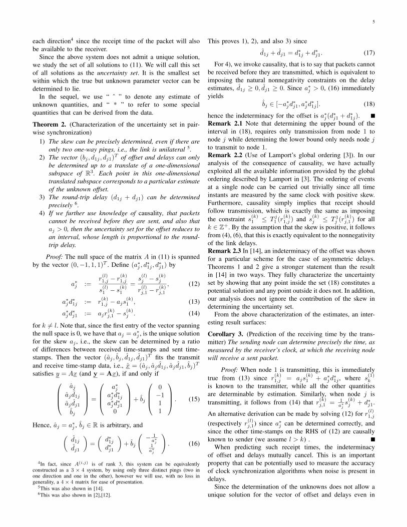
c) Complete Graph d) Connected Graphb) Star Grapha) General graph featuringboth directed and undirectededges
Reference Node
Fig. 2. General graph, Star graph, Complete graph, and connectedgraph
the simple case of pairwise communication, it is of interest todetermine simple additional conditions that will allow precisecharacterization of offset and delays.
Theorem 4. (Sufficient conditions for uniqueness of solution)All the parameters (aj , bj , d1j , dj1) can be uniquely deter-mined if any one of the following conditions hold:
1) The offset bj , or one of the delays d1j or dj1, is known.2) There is a known affine relationship between the delays
in the two directions, specifically, there exist α 6= −1, βknown, such that dj1 = αd1j + β.
Proof: The first part follows directly from the fact thatdelays are known invertible (since aj 6= 0) affine functions ofthe offset bj (15), and the sum of the delays is known (17).To prove the second part of the theorem, we use the conditiondj1 = αd1j + β in (15) and get the unique solution
ajd1j
dj1bj
=
a∗j
(d∗1j+d∗j1)−β1+α
α(d∗1j+d∗j1)+β
1+α
a∗jαd∗1j−d
∗j1+β
1+α
. (19)
Remark 4.1 The affine characterization of asymmetry inTheorem 4.2, includes the special case of symmetric delaysd1j = dj1, which was established in [2], [12]. It alsoincludes the case of known asymmetry, dj1 − d1j = β, whichcorresponds to a known processing overhead in one of thenodes. More generally, studying the asymmetry as in [9] canlead to a full characterization of the pairwise problem. Ananalysis based on a decomposition of delays is given in SectionVIII.Remark 4.2 (Worst case error in NTP is proportional to round-trip delay). Consider two clocks which are bidirectionallyconnected, that is both can send packets to each other. InNTP, the offset is estimated based on the assumption that thedelays in the two directions are the same, i.e., d1j = dj1. Thiscorresponds, in the light of (19), to choosing the midpoint ofthe uncertainty interval (18), i.e., the point that minimizes themaximum error. Thus, the worst-case error of NTP is equal toaj(dj1+d1j)
2 .
V. NETWORK CLOCK SYNCHRONIZATION
Now we turn to the case of networks. We consider a networkof n nodes where, again by convention, node 1 is consideredto be the reference node. We will draw a directed edge fromnode i to node j if i can send packets to j. We will drawan undirected edge if both i and j can send packets to
each other; see Figure 2a. We will call the resulting graphthe communication graph. We will also occasionally refer todirected edges as unidirectional or unilateral links, and toundirected edges as bilateral or bidirectional links.
To motivate and set the stage for the general results tofollow, consider the star communication graph shown inFigure 2b, where all nodes are only allowed to bilaterallyexchange packets with the reference node. This is equivalentto having (n − 1) independent pairwise “synchronizations.”From the results of the previous section, it follows immedi-ately that determining all parameters is infeasible. There areexactly (n − 1) degrees of freedom in the uncertainty set ofthe 4(n − 1)-dimensional unknown parameter vector. Thesecorrespond precisely to the estimates of the unknown offsetsof the (n− 1) clocks with respect to the reference clock. Thedelay estimates are in turn characterized as affine functions ofthese offset estimates.
In the general multi-node case, where the graph does notnecessarily correspond to a star, our goal is to similarlydetermine what is or is not determinable when the nodesare allowed to collaborate, i.e., when nodes other than thereference node communicate with one another. An extremesituation is when all nodes are allowed to exchange packetsbilaterally with one another, i.e., the case of a completecommunication graph (see Figure 2c). We will show that evenwith such full collaboration the uncertainty set remains exactlythe same as in the star graph, if causality is not invoked. Infact we will show that the same uncertainty set results for anydirected synchronization graph that is connected (see Figure2d). In the sequel we will build up to this general case .
We first consider the problem of synchronization betweentwo nodes neither of which is the reference node.
Corollary 5. (Pairwise synchronization between two nodesother than the reference node0 In pairwise synchronizationbetween two nodes i and j neither of which is the referencenode 1, the same impossibility results and structure of theuncertainty set presented in the previous section hold, withthe relative skew aj
aitaking the place of the skew aj , and the
relative offset bj − ajaibi in place of the offset bj .
Proof: In order to define a linear system of equations,we consider the parameters {ajai , ajdij , ajdji, bj −
ajaibi} as
unknowns in the estimation problem. This yields exactly thesame system of equations as (10),
r(1)i,j
s(1)j
r(2)i,j
s(2)j...
=
s
(1)i 1 0 1
r(1)j,i 0 −1 1
s(2)i 1 0 1
r(2)j,i 0 −1 1...
......
...
ajai
ajdijajdji
bj − ajaibi
. (20)
Therefore the previous results continue to hold for this newparametrization.
Note that, as earlier, three noiseless alternating communi-cation pings per link suffice for estimation. We can consideragain a 4 × 4 system of rank 3, derived from (20) byconsidering four distinct alternating communication pings asshown in Figure 1. For compactness of representation we
7
denote this system, which contains all the information for thepair (i, j), by
y(i,j) = A(i,j)x(i,j),
where x(i,j) := (ajai, ajdij , ajdji, bj −
ajaibi)
T . (21)
Thus, generalizing the earlier result in Theorem 2, therelative skew aj
aican therefore be determined correctly, while
there is no unique solution for the unknown link delays dij , djiand relative offset bj − aj
aibi. Moreover, due to the occurrence
of the product ajdij in this parametrization, in order to expressthe unknown delays as affine functions of the relative offsetbj − aj
aibi, we need to have first determined the skew aj . This
is a network issue when node j does not have a direct linkwith the reference node 1, and we now turn to this issue.
A. Skew estimation in networks
In a unilateral communication link (i, j), relative skew canbe determined correctly by the exchange of two noiselesspings, by
ajai
=r
(l)i,j − r
(k)i,j
s(l)i − s
(k)i
. (22)
We will consider two cases for the knowledge that nodeshave:
1) Genie. We assume that there is a centralized viewof the entire network, i.e., a genie that is aware ofthe transmitter time-stamp and the receiver time-stampof every packet exchange between any pair of nodes.This implies, that links do not have to be bilateral forskew estimation, since communication in one directionsuffices for the estimation of relative skew through (22).The genie scenario serves as an absolute upper boundon what can be determined.
2) Network. This is the scenario of actual interest whereeach node knows only the information that it transmitsor that is transmitted to it by packets. Such packets,as noted in Section IV, can contain the transmitter’stime-stamp, as well as information that the transmitterhas obtained from packets it has received. Note thatcommunication along the unilateral link (i, j) impliesthat only the receiving node j can determine correctlythe relative skew via (22), but the transmitter i isunaware of the relative skew (unless it is provided thatinformation by some other path).
Concerning the communication graph of the network, wesuppose that there is a directed graph with node set Nand edge set E . In the sequel, we say that there is anundirected path from i to j, if there is a set of nodes(i0 = i, i1, . . . , il = j) such that for every 1 ≤ m ≤ l, either(im−1, im) ∈ E or (im, im−1) ∈ E , or both. We say that thereis a directed path from node i to node j if there is a set ofnodes (i0 = i, i1, . . . , il = j), such that each directed edge(im−1, im) belongs in E for 1 ≤ m ≤ l.
Theorem 6. (Necessary and sufficient network topology forthe estimation of all nodal skews) Consider a network of nnodes.
1) In the genie case, all the skews {ai}ni=2 can be deter-mined correctly if and only if there is an undirected pathfrom the reference node to every node in the networkgraph, i.e., if the graph is connected.
2) In the network case, every node in the network candetermine its own skew (relative to the reference) if andonly if there is a directed path from the reference nodeto that node, i.e., if and only if the graph contains adirected spanning tree rooted at the reference.
3) In the network case every node in the network candetermine all nodal skews (and therefore all relativeskews) if and only if there is a directed path from everynode to all nodes, i.e., if the graph is strongly connected.
Proof:1). Sufficiency is immediate since the skew of any node can
be computed by multiplying the relative skews of the nodesalong a path connecting it to the reference. Necessity followsbecause if the graph is disconnected, then there are i > 1connected components, say N1, N2, . . . , Ni, such that thereis no packet exchange between any two components. Thenmultiplying the skew of all the clocks in component Nk bya positive integer θk, for k = 1, 2, . . . , i, would create noinconsistency with any of the time-stamps.
2). For sufficiency, consider a directed path (i0 =1, i1, . . . , il = j) from the reference node to node j. Thennode im (1 ≤ m ≤ l) can determine the ratio aim
aim−1from
its incoming packets along link (im−1, im) and communicatethat ratio to all nodes ip for p ≥ m + 1 by including thatinformation in its outgoing packets. Node il = j simply formsthe product ail
ail−1
ail−1
ail−2· · · ai1ai0 =
aja1
. To prove the necessity,let N1 be the set containing node 1 and the set of nodes forwhich there is a directed path from node 1 to every node in theset, and N2 := N\N1. If N2 is not empty, we can multiplythe skew of all nodes in N2 by θ, in consistency with thetransmit time-stamps of packets sent by nodes in N2 and thereceipt time-stamps of packets received by nodes in N2.
3). Sufficiency follows, since for any distinct nodes i and j,node j can determine its relative skew to node i by multiplyingthe relative skews along a directed path to j rooted at node i,as in the proof of sufficiency in 2). The proof of necessity isas in 1), applied to strongly connected components.
We note that an important special case that satisfies all theconditions of the above theorem is when all the links arebidirectional and the network is connected.
VI. CHARACTERIZATION OF SYNCHRONIZABILITY INNETWORKS
Now we are ready to address what is feasible or infeasiblefor the problem of synchronizing clocks over networks. First,we note that in a network with n nodes and link set E ofdirected edges, there are a total of 2(n − 1) + |E| unknownparameters {ai, bi}ni=2 and {dij}(i,j)∈E . If the graph is com-plete, i.e., all nodes can bilaterally exchange packets withone another, then the number of unknowns in the networksynchronization problem is 2(n−1)+n(n−1) = (n+2)(n−1).
The following theorem establishes the fundamental resultthat without any further assumptions, clock synchronization is

8
impossible in any network.
Theorem 7. (Infeasibility of clock synchronization in net-works) Consider a network of n nodes. It is impossible todetermine all 2(n− 1) + |E| unknown parameters {ai, bi, anddij for all i and all j : (i, j) ∈ E} even if all pairs of nodescan exchange any number of time-stamped packets containingany information that is causally known to the transmitter.
The next theorem characterizes the uncertainty set of theunknown parameters.
Theorem 8. (Characterization of the uncertainty set in net-work clock synchronization) Consider any network topologyG := (N , E) such that in E there is a directed path from anynode to any other node, i.e., G is strongly connected.
1) All the skews {ai : 2 ≤ i ≤ n} can be determinedcorrectly.
2) Every vector d = (dij , (i, j) ∈ E) in the uncertaintyset for the delay vector d = (dij , (i, j) ∈ E) can beexpressed as a known affine transformation of (n − 1)variables {bi : 2 ≤ i ≤ n}. Each bi can be regardedas an estimate of the unknown offset bi. Any choice ofthese estimates {bi : 2 ≤ i ≤ n} is consistent with alltransmit and receipt time-stamps of all packets.
3) If causality is invoked, the uncertainty set for the esti-mates of the offset parameters {bi : 2 ≤ i ≤ n} can befully characterized as a compact polyhedron of Rn−1.
4) Suppose all links in E are bilateral. Then the feasiblepolyhedron in 3 has a non-empty interior if and only ifthere is no bilateral link with zero round-trip delay.
Remark 8.1 An important consequence is that the star graphand, in general, any spanning tree, results in the same uncer-tainty set for the parameters as the complete graph, if causalityis not invoked. If causality is additionally taken into account,then additional communication links do help to reduce the sizeof the uncertainty set.
Proof of Theorems 7, 8: Theorem 8.1 is just a restatementof Theorem 6.3.
We will first prove Theorem 7 and Theorem 8.2 together,under the best case scenario of a complete graph, i.e., whenall links are active and |E| = n(n− 1). Subsequently we willshow that the conclusion of Theorem 8.2 continues to hold forany strongly connected graph where there is a directed pathfrom any node to any other node.
The complete graph contains the star graph for which wealready know that the conclusions of Theorem 7 and Theorem8.2 hold. Thus, to show Theorem 7 and Theorem 8.2 for thecomplete graph, it suffices to show that any estimate in theuncertainty set for the star graph will also satisfy the datafrom all bilateral packet exchanges, and to further express thelink delays {dij} for i, j 6= 1 as affine functions of the offsetestimates {bi}ni=2.
In order to tackle the difficulties of a nonlinear parametriza-tion, we introduce a redundant parametrization, with respect towhich the system of equations to be solved becomes linear. Anatural selection, as in Corollary 5, is to choose the parameters{ajai , ajdij , ajdji, bj −
ajaibi} for i = 2, 3, . . . , n, and j = i+
1, i+ 2, . . . , n, and {aj , ajd1j , ajdj1, bj} for j = 2, 3, . . . , n,since a1 = 1, b1 = 0. From the fact that there are n(n−1)
2communicating pairs of nodes i and j with i < j, thisparametrization involves 4n(n−1)
2 = 2n(n − 1) parameters.It is redundant, for n > 2, since the number of the parametersis more than the (n + 2)(n − 1) unknowns. Hence, we haveintroduced an additional (n−1)(n−2) redundant parameters,but this over-parametrization has the advantage that not onlydoes the system become linear as before in the two-nodesystem, but also fully decoupled in the communicating pairs.Using (21) and taking four alternating pings, the whole systemcan be put in block diagonal matrix form:
y(1,2)
...y(i,j)
...y(n−1,n)
=
A(1,2) · · · O · · · O...
. . ....
......
O · · · A(i,j) · · · O...
......
. . ....
O · · · O · · · A(n−1,n)
x(1,2)
...x(i,j)
...x(n−1,n)
,
(23)
The blocks A(i,j) are 4× 4 matrices as given by (11) and thefirst four rows of (20), while O is the 4× 4 zero matrix7. Wedenote this system, by slight abuse of notation, by y = A x.
The dimension of the square matrix A is 2n(n − 1) ×2n(n−1). This matrix however has rank only 3n(n−1)
2 since allthe blocks in the diagonal have rank three and four columns.We cannot yet conclude non-uniqueness of solution since theparametrization itself is redundant.
By the results in (15) of Theorem 2, which, as weshowed in Corollary 5, carry over for the parameters{ajai , ajdij , ajdji, bj −
ajaibi}, we have
(ajai
)
(ajdij)
(ajdji)(bj − aj
aibi)
=
(ajai
)∗
(ajdij)∗
(ajdji)∗
0
+ θij
0−111
, (24)
with (ajai
)∗ :=r
(l)i,j − r
(k)i,j
s(l)i − s
(k)i
=s
(l)j − s
(k)j
r(l)j,i − r
(k)j,i
=ajai,(25)
(ajdij)∗ := r
(k)i,j −
ajais
(k)i , (26)
(ajdji)∗ :=
ajair
(k)j,i − s
(k)j . (27)
The vector in the LHS of (24) denotes estimates, parametrizedby a selection of the one degree of freedom θij . The quantitiesin the first vector on the RHS of (24) can be determined bytwo time-stamped packets k and l sent from node i to nodej, and one packet sent from node j to node i, or vice-versa.In fact, if we further define
a∗j := aj , (28)
d∗ij :=1
ajr
(k)i,j −
1
ais
(k)i . (29)
then (ajdij)∗ = a∗jd
∗ij and (
ajai
)∗ =a∗ja∗i
. We will denote
7The matrices A(i,j) are considered to be 4× 4 without loss in generality.However, any one of them can be constructed as a 3× 4 matrix as shown inRemark 1.1.

9
the system in (24) by x(i,j) = x∗(i,j) + θijn, where θij :=(bj − aj
aibi) and n := (0,−1, 1, 1)T .
Since the estimation of all the unknown parameters inthe network has been decoupled in (23) into estimations forseparate links, we have
x :=
x(1,2)
...x(i,j)
...x(n−1,n)
=
x∗(1,2)
...x∗(i,j)
...x∗(n−1,n)
+ θ12
n
...0
...0
+ · · ·+ θn−1,n
0
...0
...n
, (30)
where 0 := (0, 0, 0, 0)T . All solutions for x consistent withthe data of transmit and receipt time-stamps of all packets areof the form (30).
Now we need to determine what is the freedom in the valuesof the parameters {θij : 1 ≤ i < j ≤ n}, so that one canchoose {ai, bi, dij} to satisfy (
ajai
) =ajai, (ajdij) = aj dij ,
and (bj − ajaibi) = bj − aj
aibi. It is plain to check that these
constraints give a set of (n−1)(n−2) equations, and also noother constraints exist, hence, the redundancy in the systemwill be eliminated.
First, from Theorem 6.3 we see that ai = ai for all i sincethe skews can be correctly determined, hence the (n−1)(n−2)
2
equations (for the case of a complete graph) (ajai
) =ajai
willprovide no additional constraints on {θij : 1 ≤ i < j ≤ n}.
Next, θij := (bj − ajaibi) = bj − aj
aibi = bj − aj
aibi, which
yields (n−1)(n−2)2 independent equations, so that the “free”
parameters {θij} are linear functions of the offset estimates{bi : 2 ≤ i ≤ n}. Hence there are only (n − 1) independentparameters {bi : 2 ≤ i ≤ n} that determine the values of allthe θij for i < j.
Next, from the equations defined by the second and thirdrow in (24), since ai = ai and θij = bj − aj
aibi we obtain, in
both cases i < j as well as j < i, that
dij = d∗ij +1
aibi −
1
ajbj . (31)
Hence we see that all delay vectors in the uncertainty set canbe affinely characterized by exactly (n−1) remaining degreesof freedom {bi}ni=2, which are the estimates for the offsets. Inconsequence, the estimation problem does not yield a uniquesolution, proving Theorem 7. Moreover, the uncertainty set ofthe parameter vectors in the network is an affine transformationof an (n−1)-dimensional subspace. This proves Theorem 8.2for the case of a complete graph. However, a perusal showsthat this proof also generalizes to the case where the link set Eallows all skews to be determined, and the latter is guaranteedby Theorem 6.3.
Now we turn to Theorem 8.3. As in Theorem 2, we use theproperty that for ai > 0 causality is equivalent to dij ≥ 0 , toobtain from (31) that
1
aibi −
1
ajbj ≥ −d∗ij for all (i, j) ∈ E . (32)
which characterizes the uncertainty set for offsets.
We now show that the uncertainty set is compact. Startingfrom node i, there is a directed path to the reference node 1.So applying (32) repeatedly, and using b1 = 0, gives
bi ≥ ai∑
link (i,j) ∈ directed path(−d∗ij). (33)
Similarly, starting from the reference node and considering adirected path to node i one gets an upper bound
bi ≤ ai∑
link (i,j) ∈ directed pathd∗ij . (34)
To prove Theorem 8.4, we note that when all links in E arebilateral the inequality constraints in (32) are
−d∗ji ≤1
ajbj −
1
aibi ≤ d∗ij , for all (i, j) ∈ E . (35)
So a necessary and sufficient condition for the polyhedron tobe full-dimensional (n − 1), is that the upper bound in (35)strictly exceeds the lower bound, i.e., d∗ij + d∗ji > 0. Since weknow that this is equal to the round-trip delay dij + dji, theresult follows.Remark 8.2 There are only (n− 1) free parameters that onecan choose if one wants the estimate to be consistent with alltransmit and receipt time-stamp data. This shows that whilein pairwise synchronization unknown delay asymmetry is theunique reason for indeterminacy (that is to say assuming thatdelays are symmetric there is no indeterminacy left), in thenetwork case (n > 2), this is not the case any more. Toillustrate this effect, suppose that all communication links arebilateral, and hence the network topology is modeled by anundirected graph (N , E), and link delays are not symmetric,but yet we assume they are. Then the assumption results in|E| additional constraints which may exceed the number ofthe free parameters (n− 1), and one will be unable to choosesymmetric delay estimates that are consistent with the data.This has also been observed in [12].Remark 8.3 In [12], the special case where all clocks runat the same speed, all links are bilateral, and there exists aspanning tree, is examined. If we denote the set of all directedcyclic paths of the graph (N , E) by C, then by invokingcausality, it is shown in [12] that the delay vector d lies in theintersection of the positive orthant R|E|+ and the hyperplanes∑
(i,j)∈C
dij =∑
(i,j)∈C
d∗ij for all C ∈ C. (36)
The latter also follows immediately from (31). It is also shownin [12] that all link delays can be expressed as known affinefunctions of the (n − 1) delays of the links of a directedspanning tree rooted at the reference node. This arises alsoas a plain corollary of our analysis, since the affine mappingrelating the delays of the links of a directed spanning treeand the nodal offsets is invertible. The latter, in conjunctionwith the sharp characterization of the uncertainty set inTheorem 8, imply that the uncertainty set for link delays iscompletely characterized as the intersection of R|E|+ and theset in (36). However our analysis does not require all linksto be bidirectional, nor all skews to be identical, nor doesit depend on finding a spanning tree. Most importantly, we
10
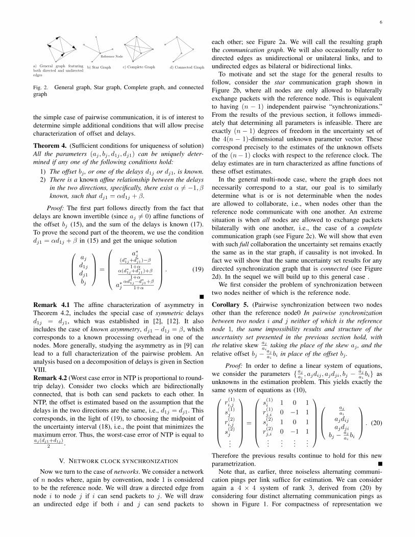
Node m
Node i
Node j
r(k)m,i
r(k)m,j
r(l)m,i
r(l)m,j
Fig. 3. Receiver-receiver synchronization
have shown that the number of degrees of freedom is exactlyequal to (n− 1), thus fully characterizing the uncertainty setfor both offsets and delays, whereas in [12] the set in (36) isonly shown to be necessary but not sufficient. Additionally,no constraints on the offsets are provided in [12].Remark 8.4 (Choosing an estimate in the offset feasible set)Since the offsets cannot be exactly determined, one may beinterested in a min-max estimate. We pose the problem asone of finding the smallest hyper-rectangle that contains thepolyhedron that characterizes the offset uncertainty set, withthe estimate then chosen as the center of the hyper-rectangle.This can be obtained by solving the Linear Program:
max∑ni=1(b
(i)i − b
(i)i ) (37)
s.t. 1aib(k)i − 1
ajb(k)j ≥ −d∗ij , k = 1, · · · , n, (i, j) ∈ E ,
1aib(k)i − 1
ajb(k)j ≥ −d∗ij k = 1, · · · , n, (i, j) ∈ E ,
and estimating the offsets by b∗i =b(i)i +b
(i)i
2 for 2 ≤ i ≤ n,where b(k)
i denotes the i-th component of the vector b(k) ∈Rn−1, and b(k)
i denotes the i-th component of the vector b(k) ∈Rn−1. It would be of interest to obtain a distributed algorithmto determine such {b∗i , 2 ≤ i ≤ n}.Remark 8.5 The derivation of the uncertainty set naturallygeneralizes to the case that multiple nodes are assumed to be“synchronized” by letting ai = 1, bi = 0 for all such clocks.The case that a node has a “known” offset bi can be treatedanalogously.
VII. RECEIVER-RECEIVER CLOCK SYNCHRONIZATION
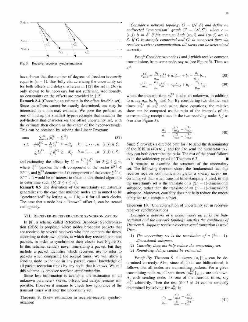
In [8], a scheme called Reference Broadcast Synchroniza-tion (RBS) is proposed where nodes broadcast packets thatare received by several receivers who then compare the times,according to their own clocks, at which they received commonpackets, in order to synchronize their clocks (see Figure 3).In this scheme, senders never time-stamp a packet, but theyinclude a packet identifier which receivers use to refer topackets when comparing the receipt times. We will allow asending node to include in any packet, causal knowledge ofall packet reception times by any node, that it knows. We callthis scheme as receiver-receiver synchronization.
Since less information is available, the estimation of allunknown parameters skews, offsets, and delays remains im-possible. However it remains to check how ignorance of thetransmit times will alter the uncertainty set.
Theorem 9. (Skew estimation in receiver-receiver synchro-nization)
Consider a network topology G = (N , E) and define anundirected “comparison” graph G′ = (N , E ′), where e =(i, j) is in E ′ if for some m both (m, i) and (m, j) are inE . If G is strongly connected and G′ is connected then viareceiver-receiver communication, all skews can be determinedcorrectly.
Proof: Consider two nodes i and j which receive commontransmissions from some node, say m (see Figure 3). Then weget
r(k)m,i =
aiam
s(k)m + aidmi + bi −
aiam
bm, (38)
r(k)m,j =
ajam
s(k)m + ajdmj + bj −
ajam
bm, (39)
where the transmit time s(k)m is also an unknown, in addition
to ai, aj , am, bi, bj , and bm. By considering two distinct senttimes s
(k)m 6= s
(l)m and using these equations, the relative
skew can be computed as the ratio of the intervals of thecorresponding receipt times in the two receiving nodes i, j as(see also Figure 3),
ajai
=r
(l)m,j − r
(k)m,j
r(l)m,i − r
(k)m,i
. (40)
Since E provides a directed path for i to send the denominatorof the RHS in (40) to j, and for j to send the numerator to i,they can both determine the ratio. The rest of the proof followsas in the sufficiency proof of Theorem 6.2.
It remains to examine the structure of the uncertaintyset. The following theorem shows the fundamental fact thatreceiver-receiver communication yields a strictly larger un-certainty set than when transmit time-stamping is used, in thatthe uncertainty set is the translate of a (2n − 1)-dimensionalsubspace, rather than the translate of an (n − 1)-dimensionalsubspace. Moreover, causality does not help reduce the uncer-tainty set to a compact subset.
Theorem 10. (Characterization of uncertainty set in receiver-receiver synchronization)
Consider a network of n nodes where all links are bidi-rectional and the network topology satisfies the conditions ofTheorem 9. Suppose receiver-receiver synchronization is used.Then,
1) The uncertainty set is the translation of a (2n − 1)-dimensional subspace.
2) Causality does not help reduce the uncertainty set.3) Round-trip delays cannot be estimated.
Proof: By Theorem 9 all skews {ai}ni=2 can be de-termined correctly. Also, since all links are bidirectional, itfollows that all nodes are transmitting packets. For a giventransmitting node m, all sent times {s(k)
m }k∈Z+ are unknown.At each sending node, fix one of the transmit times, says
(k)m arbitrarily. Then the rest (for l 6= k) can be uniquely
determined by solving for s(l)m in
aiam
=r
(l)m,i − r
(k)m,i
s(l)m − s(k)
m
. (41)
11
This gives n degrees of freedom, one for each node, in makingchoices for estimates of transmit times. Once these n degreesof freedom are fixed, all sent times are known and the resultsof Theorem 8 apply, and provide (n − 1) additional degreesof freedom. Therefore 1) follows. To determine the affinetransformation, define
d∗mi :=1
air
(k)m,i −
1
ams(k)m , (42)
and exploiting (38) we get
dmi = d∗mi +1
ambm −
1
aibi. (43)
This constitutes a solution for every choice of {bi : 2 ≤ i ≤n}. This is the set of all solutions, since the true solution doesindeed originate from a particular choice of transmit times. Infact, for nodes, i, and j, receiving common packets, (38), (39)give
dmi − dmj = (1
air
(k)m,i −
1
ajr
(k)m,j)−
1
aibi +
1
ajbj . (44)
i.e., we have eliminated all unknown sent times. These equa-tions, for all links (i, j) ∈ E ′, completely characterize theuncertainty set, since for any solution they admit, a networksolution can be obtained by properly determining the n degreesof freedom corresponding to sent times, through (42) and (38).
2) This is immediate from the fact that causality is equiv-alent to the non-negativity of delays. However, in (44) thedelays appear in differences (44), so no sign constraint can beimposed on these differences. Even though we have
1
aibi −
1
ambm ≤ d∗mi, (45)
d∗mi can be made arbitrarily large by choosing s(m)k in (42)8.
3) This follows since the round-trip delay dij +dji is equalto d∗ij + d∗ji, but the latter cannot be uniquely chosen.Remark VII.1 Suppose all receiver delays are equal, i.e.,dmi = dmj for all m, i, j for which node m transmits tonodes i, j. Then from (44),
bj −ajaibi = r
(k)m,j −
ajair
(k)m,i. (46)
So the relative skew bj − ajaibi can be determined since the
quantities on the RHS are known. Schemes such as RBSimplicitly assume equality of delays. However, such equalitymight not provide a network-wide consistent solution, sincethe number of constraints to be enforced might be more thanthe number of free parameters.
VIII. ANALYSIS OF STRUCTURED MODELS OF LINKDELAYS
We now study the case where link delay has additionalstructure. We obtain a sufficient condition for correctnessof estimates. We also provide an example where a correctestimate is attainable, and one where it is not. Moreover,we demonstrate a model where the uncertainty set of the
8Not all such bounds can be arbitrarily made large simultaneously, sincethe number of links might be larger than the total degrees of freedom.
delays is characterized by only one or two degrees of freedom,in contradistinction to the (n − 1) degrees of freedom inthe general case. This is important since the number of theremaining degrees of freedom is then constant, independentof the network size.
A decomposition of the packet delivery delays was firstintroduced in [10]. We will suppose that the delay in thedirected communication pair (i, j), dij , consists of the sumof three terms:
1 . A transmission delay αi which accounts for the pro-cessing time in the transmitter after time-stamping. This isassumed to be fixed and transmitter-dependent. This includes,in the terminology of [10], the “Send Time,” the time usedto construct the message at the application layer and transferit to the MAC layer on the transmitter side, as well as the“Access Time,” the delay incurred waiting for access to thetransmit channel up to the point when transmission begins,and the “Transmission Time,” the time it takes for the senderto transmit the message bit by bit at the physical layer.
2. An electromagnetic propagation delay τij which can beestimated correctly, say by GPS, or other position information,since it only involves the distance between the nodes, and ishence assumed known.
3. A receiving delay βj which accounts for the processingtime in the receiver before time-stamping. This is also assumedto be fixed and receiver-dependent. This includes, in theterminology of [10], the “Reception Time,” the time takenin receiving the bits and passing them to the MAC layer, andmay include an overlap with Transmission Time, as well as the“Receive Time,” the time it takes to reconstruct the incomingbits into a packet and pass it to the application layer where itis decoded.
To sum up, the model for the delay is
dij = αi + τij + βj , i, j = 1, 2, . . . , n and i 6= j. (47)
The important point is that by exploiting such a decomposition,the number of unknowns for the delays reduces from n(n−1)to 2n in the case of a complete graph, since we need onlyestimate the variables {(αi, βi) : 1 ≤ i ≤ n}. Let us denotetheir estimates by {(αi, βi) : 1 ≤ i ≤ n}.
From (31) we see that the delay vector d ∈ R|E| can beexpressed as an affine function of the offset vector b ∈ Rn−1:
d = d∗ +Bb, B ∈ R|E|×(n−1), (48)
where Bem =
− 1a∗j, m+ 1 = j,
1a∗i, m+ 1 = i,
0, else.
(49)
where e is used to denote the directed link (i, j) for notationalconvenience in the matrix representation, and d∗ is the vectorcontaining the values d∗ij as given by equations (13), (14),(29).
However, from the structured model assumption for the

12
delays (47) we have
d = Dθ + τ , θ ∈ R2n, D ∈ R|E|×2n, (50)
where Dem =
{1 if m = i or m = n+ j,0, else.
(51)
θi =
{αi, i = 1, 2, . . . , n.
βi−n i = n+ 1, . . . , 2n.(52)
The vector τ is a known vector with entries being the elec-tromagnetic propagation delays {τij , (i, j) ∈ E}. Notice thatthe matrix D is of full column rank 2n. This is easy tosee by observing that the rows corresponding to the delays{d12, d13, . . . , d1n, dn1, d21, d31, . . . , dn−1,1, d23, d32} form aset of 2n linearly independent vectors.
Substituting (50) into (48), we get
Dθ = c+Bb, (53)
where c := d∗ − τ is a known vector.
Lemma 11. (Non-uniqueness of solution in the structureddelay model) The solution for θ in (53) is not unique. Hence,in general, the structured delay case is still unsolvable.
Proof: Adding ε > 0 small enough to all αi’s andsimultaneously subtracting the same value ε from all βi’sleaves (53) invariant.
More generally one may have other specific models for thedelay.
Lemma 12. (Necessary and sufficient condition for unique-ness of solution in structured delay models)
Suppose all links are bidirectional and all round-trip delaysare strictly positive. Suppose the delay vector satisfies an affinerelationship d = Aα + β where A, β are known, and A hasfull rank. Then, there exists a unique d that satisfies both d =Aα + β for some α, as well as d = d∗ + Bb, if and only ifATB = 0.
Proof: Substituting d = Aα+ β into (48) we have
Aα = c+Bb, (54)
where c := d∗ − τ is a known vector.Since A has full rank, the matrix (ATA) is square and non-
singular. Hence the pseudo-inverse of A, defined by A# :=(ATA)−1AT exists, and satisfies A#A = I, where I denotesthe identity matrix. We then get
α = A#c+ (A#B)b. (55)
Now A#c is known, and also B has full rank. To verifythe latter, one can check that the rows corresponding to thedelays {d12, d13, . . . , d1n} form a diagonal (n− 1)× (n− 1)matrix with strictly negative values {− 1
a2,− 1
a3. . . ,− 1
an}.
Hence (A#B) is also of full rank. A unique solution existsif and only if (A#B)b = 0. The feasible set of the vectorof offset estimates, b, is Rn−1 or, if causality is invoked, apolyhedron. In both cases, these sets have non-empty interior,i.e., full dimension n − 1. Thus, the condition (A#B)b = 0for all “feasible” vectors b, reduces to (A#B) = 0, which isequivalent to ATB = 0.
Example. Consider the case where there is an unknown affinerelation between the transmit and receive delay, i.e., αi =γβi + δ for all nodes, where the parameters γ, δ are unknownand γ > 0. For each fixed pair (γ, δ), we obtain a knownaffine characterization of the asymmetry. Hence there exists aunique solution by Theorem 4. As one ranges9 over variousγ > 0 and δ, one obtains an uncertainty set parametrized bytwo degrees of freedom, namely γ, δ.
An interesting special case is when δ = 0. This correspondsto the case where nodes run at a constant but unknown speed,and transmitting and receiving delays are simply inverselyproportional to the speed of the processor at the node. In thiscase, the uncertainty set is parametrized by a single degree offreedom, γ > 0.
IX. CONCLUDING REMARKS
We have characterized what is fundamentally feasible andinfeasible in synchronizing clocks over wired or wirelessnetworks. The main result is that the determination of theunknown clock offsets, and the link delays is, in general,impossible, though the skews can be determined correctly. Wehave also characterized the uncertainty set. The delays can beestimated up to one unknown offset for each node except thereference node, with these nodal offsets being indeterminableparameters. Invoking causality, the offset vector lies in acompletely characterized polyhedron. We also have providednecessary and sufficient conditions on the network topologyfor this polyhedron to be compact and have a non-emptyinterior. If there is a known asymmetry in the delays that canbe affinely characterized, a unique solution exists. Despite theuncertainty in offset and delay, a sender can predict exactly thetime its packet will be received, as measured by the receiver’sclock. For the problem of receiver-receiver synchronization,the nodal skews can still be determined correctly but onlydelay differences between neighboring communication linkswith a common sender can be expressed affinely with respectto the (n − 1) unknown offsets. Causality does not reducethe uncertainty set which remains unbounded. Last, we havestudied the special case where the link delays have structure interms of transmit and receipt delays plus known electromag-netic propagation times, and provided sufficient conditions foruniqueness of solution.
ACKNOWLEDGMENT
This material is based upon work partially supported byNSF under Contract Nos. ECCS-0701604, CNS 05-19535and CCR-0325716, Oakridge under DOE BATT 4000044522,DARPA/AFOSR under Contract No. F49620-02-1-0325, andAFOSR under Contract No. F49620-02-1-0217. Any opinions,findings, and conclusions or recommendations expressed inthis publication are those of the authors and do not necessarilyreflect the views of the above agencies.
9Note that all values of γ > 0 are feasible, but for given γ, δ is boundedabove by the fact that round-trip delays in bilateral links are known byestimation.

13
REFERENCES
[1] N. Freris and P. R. Kumar, “Fundamental Limits on Synchro-nization of Affine Clocks in Networks.” Proceedings of the 46thIEEE Conference on Decision and Control, pp. 921-926, NewOrleans, Dec. 12-14, 2007.
[2] S. Graham and P. R. Kumar, “Time in general-purpose controlsystems: The Control Time Protocol and an experimental eval-uation.” Proceedings of the 43rd IEEE Conference on Decisionand Control, pp. 4004-4009. Bahamas, Dec. 14-17, 2004.
[3] L. Lamport, “Time, Clocks and the Ordering of Events in aDistributed System.” Communications of the ACM, vol. 21, no.7, pp. 558-565, July 1978.
[4] R. Solis, V. Borkar and P. R. Kumar, “A New Distributed TimeSynchronization Protocol for Multihop Wireless Networks.” Pro-ceedings of the 45th IEEE Conference on Decision and Control,pp. 2734-2739, San Diego, Dec. 13-15, 2006.
[5] A. Giridhar and P. R. Kumar, “Distributed Clock Synchronizationover Wireless Networks: Algorithms and Analysis.” Proceedingsof the 45th IEEE Conference on Decision and Control, pp. 4915-4920, San Diego, Dec. 13-15, 2006.
[6] J. Elson, R.M. Karp, C.H. Papadimitriou and S. Shenker, “GlobalSynchronization in Sensornets.” Proceedings of LATIN, vol.2976, pp. 609-624, 2004.
[7] D. L. Mills, “Internet Time Synchronization: The Network TimeProtocol.” IEEE Trans. Communications, vol. 39, no. 10, pp.1482-1493, Oct. 1991.
[8] J. Elson, L. Girod and D. Estrin, “Fine-Grained Network TimeSynchronization using Reference Broadcasts.” Proceedings of theFifth Symposium on Operating Systems Design and Implemen-tation (OSDI 2002), pp. 147-163, Boston, Dec. 2002.
[9] M. Maroti, G. Simon, B. Kusy, and A. Ledeczi, “The FloodingTime Synchronization Protocol.” Proceedings of the Second In-ternational Conference on Embedded Networked Sensor Systems,Baltimore, USA, pp. 39-49, Nov. 2004.
[10] H. Kopetz and W. Ochsenreiter, “Clock Synchronization in Dis-tributed Real-Time Systems.” IEEE Transactions on Computers,C-36(8), p. 933-939, Aug. 1987.
[11] D.W. Allan, “Time and Frequency (Time-Domain) Charac-terization, Estimation, and Prediction of Precision Clocks andOscillators.” IEEE Transactions on Ultrasonics, Ferroelectrics,and Frequency Control, UFFC-34, 647-654, 1987.
[12] O. Gurewitz, I. Cidon and M. Sidi, “One-way delay estimationusing network-wide measurements.” IEEE/ACM Transactions onNetworking, vol. 14 , pp. 2710-2724, June 2006.
[13] J. Lundelius and N. Lynch, “An upper and lower bound forclock synchronization.” Information and Control, 62(2-3) : 190–204, August/September 1984.
[14] D. Veitch, S. Babu and Attila Pasztor, “Robust synchronizationof software clocks across the internet.” Proceedings of the 4thACM SIGCOMM conference on Internet measurement, pp. 219-232, Taormina, Sicily, Italy, Oct. 25-27, 2004.
[15] N. Freris, V. Borkar, and P. R. Kumar, “A model-based ap-proach to clock synchronization.” Proceedings of the 48th IEEEConference on Decision and Control, pp. 5744 - 5749, Shanghai,December 16-18, 2009.
[16] S. Graham, “Issues in the Convergence of Control with Commu-nication and Computation.” Doctoral Thesis, University of Illinoisat Urbana-Champaign, July 2004.
[17] R. Solis, “Clock Synchronization for Multihop Wireless SensorNetworks.” Ph. D. Thesis, August 25, 2009. Department ofComputer Science, University of Illinois, Urbana-Champaign.
[18] R. Solis, J. Haas, Y. Hu and P. R. Kumar, “Design andImplementation of Secure Clock Synchronization in a WirelessSensor Network.” CSL, University of Illinois, 2010.
Nikolaos M. Freris (Member, IEEE) obtained hisDiploma in Electrical and Computer Engineeringfrom the National Technical University of Athens(NTUA) in 2005. He received M.S. degrees in Elec-trical and Computer Engineering and Mathematicsfrom the University of Illinois at Urbana-Champaignin 2007 and 2008, respectively. He received a PhDin Electrical and Computer Engineering from theUniversity of Illinois at Urbana-Champaign in 2010.Since September 2010, he has been with IBM Re-search - Zurich, Switzerland, where he is currently
working as a postdoctoral research associate in the Mathematical and Com-putational Sciences group. His research has been on wireless and sensornetworks: clock synchronization, network resource allocation, random-accessMAC, and scalable video streaming. Dr. Freris was granted a VodafoneGraduate Fellowship for 2007-2008 for research in the area of wirelesscommunication networks. He was granted the Gerondelis Foundation Awardfor excellent graduate students of Greek descent in 2010. Dr. Freris is amember of the Technical Chamber of Greece.
Scott R. Graham (Member, IEEE) obtained hisBachelors of Science degree in Electrical Engineer-ing from Brigham Young University in 1993. Hereceived an M.S. degree in Electrical Engineeringfrom the Air Force Institute of Technology in 1999and a Ph.D degree in Electrical Engineering from theUniversity of Illinois at Urbana-Champaign in 2004.He is currently an Adjunct Professor of Electricaland Computer Engineering at the Air Force Instituteof Technology. His research interests include di-rectional networks, networked control systems, and
critical network infrastructure. Dr. Graham is a member of Tau Beta Pi andEta Kappa Nu.
P. R. Kumar (Fellow, IEEE) obtained his B. Tech.degree in Electrical Engineering (Electronics) fromI.I.T. Madras in 1973, and the M.S. and D.Sc.degrees in Systems Science and Mathematics fromWashington University, St. Louis, in 1975 and 1977,respectively. From 1977-84 he was a faculty memberin the Department of Mathematics at the Univer-sity of Maryland Baltimore County. Since 1985he has been at the University of Illinois, Urbana-Champaign, where he is currently Franklin W.Woeltge Professor of Electrical and Computer Engi-
neering, Research Professor in the Coordinated Science Laboratory, Researchprofessor in the Information Trust Institute, and Affiliate Professor of theDepartment of Computer Science. He has worked on problems in game theory,adaptive control, stochastic systems, simulated annealing, neural networks,machine learning, queueing networks, manufacturing systems, scheduling,wafer fabrication plants and information theory. His current research interestsare in wireless networks, sensor networks, and networked embedded controlsystems. He has received the Donald P. Eckman Award of the AmericanAutomatic Control Council, the IEEE Field Award in Control Systems, andthe Fred W. Ellersick Prize of the IEEE Communications Society. He is amember of the US National Academy of Engineering. He has been awardedan honorary doctorate by ETH, Zurich. He was awarded a Guest ChairProfessorship at Tsinghua University, Beijing. He is also the Lead GuestChair Professor of the Group on Wireless Communication and Networking atTsinghua University, Beijing. He is an Honorary Professor at IIT Hyderabad.