Fundamentals in Biophotonics

Optogentics

Aleksandra Radenovic

aleksandra.radenovic@epfl.ch

EPFL – Ecole Polytechnique Federale de Lausanne

Bioengineering Institute IBI

23.05.2016

Optogenetics

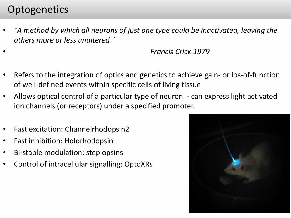
• ¨A method by which all neurons of just one type could be inactivated, leaving the others more or less unaltered ¨

• Francis Crick 1979

• Refers to the integration of optics and genetics to achieve gain- or los-of-function of well-defined events within specific cells of living tissue

• Allows optical control of a particular type of neuron - can express light activated ion channels (or receptors) under a specified promoter.

• Fast excitation: Channelrhodopsin2

• Fast inhibition: Holorhodopsin

• Bi-stable modulation: step opsins

• Control of intracellular signalling: OptoXRs

Optogenetics

• ¨A method by which all neurons of just one type could be inactivated, leaving the others more or less unaltered ¨

• Francis Crick 1979

• Refers to the integration of optics and genetics to achieve gain- or los-of-function of well-defined events within specific cells of living tissue

• Allows optical control of a particular type of neuron - can express light activated ion channels (or receptors) under a specified promoter.

• Fast excitation: Channelrhodopsin2

• Fast inhibition: Holorhodopsin

• Bi-stable modulation: step opsins

• Control of intracellular signalling: OptoXRs

Clinical application –NOT really BUT

• “Despite the enormous efforts of clinicians and researchers, our limited insight into psychiatric disease (the worldwide-leading cause of years of life lost to death or disability) hinders the search for cures and contributes to stigmatization. Clearly, we need new answers in psychiatry.”

• Karl Deisseroth

Connectome

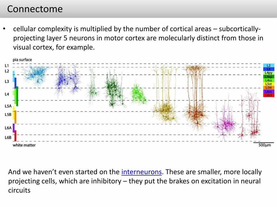
• cellular complexity is multiplied by the number of cortical areas – subcortically-projecting layer 5 neurons in motor cortex are molecularly distinct from those in visual cortex, for example.

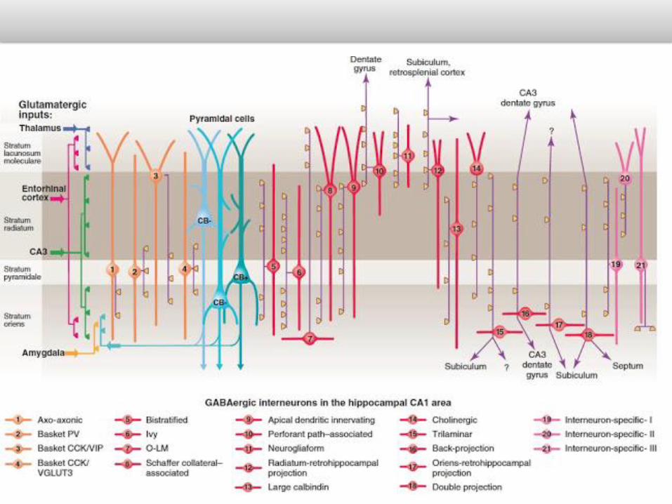
And we haven’t even started on the interneurons. These are smaller, more locally projecting cells, which are inhibitory – they put the brakes on excitation in neural circuits

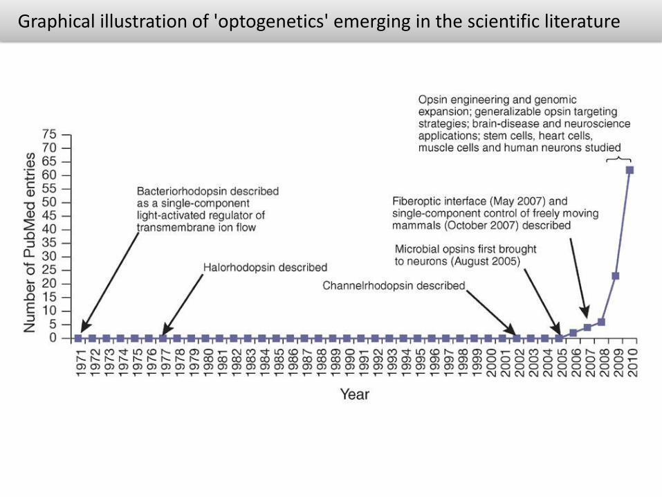
Graphical illustration of 'optogenetics' emerging in the scientific literature

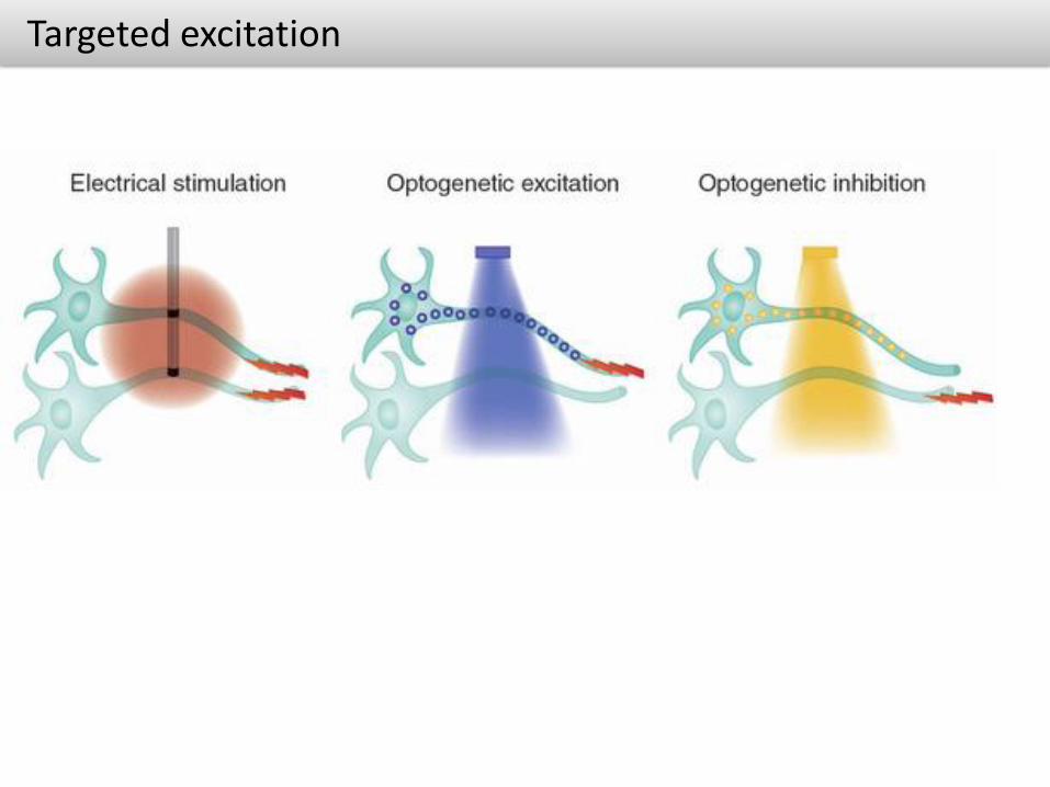
Targeted excitation

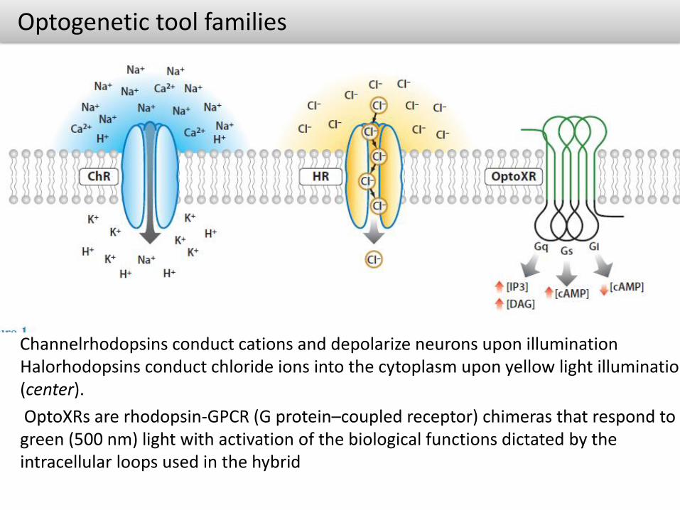
Optogenetic tool families

Channelrhodopsins conduct cations and depolarize neurons upon illumination Halorhodopsins conduct chloride ions into the cytoplasm upon yellow light illumination (center).

OptoXRs are rhodopsin-GPCR (G protein–coupled receptor) chimeras that respond to green (500 nm) light with activation of the biological functions dictated by the intracellular loops used in the hybrid

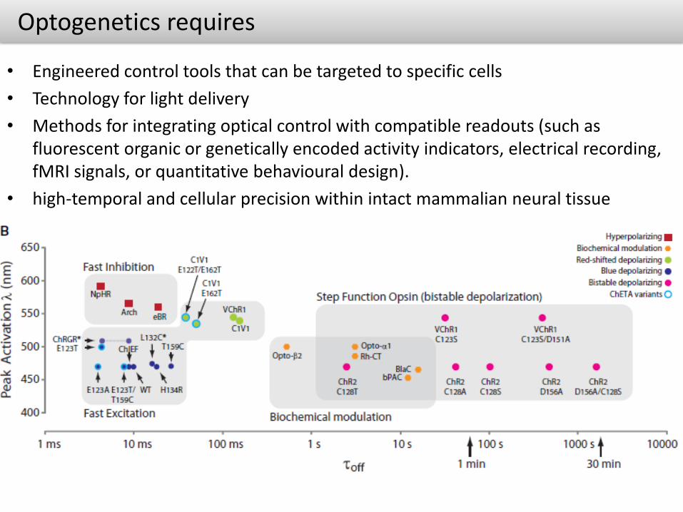
Optogenetics requires

• Engineered control tools that can be targeted to specific cells

• Technology for light delivery

• Methods for integrating optical control with compatible readouts (such as fluorescent organic or genetically encoded activity indicators, electrical recording, fMRI signals, or quantitative behavioural design).

• high-temporal and cellular precision within intact mammalian neural tissue

Advantages

• Precisely control one cell type while leaving the others unaltered (Genetically targeted to a specific group of neurons)

• Select activation of neuronal pathways (as opposed to electrical stimulation which activates many neuronal pathways)

• Fast temporal resolution: Millisecond scale precision to keep pace with the known dynamics of the targeted neural events such as action potentials and synaptic currents

• Can be operative within intact systems including freely moving animals. Can directly correlate neural activity in vitro with behaviour

Preparation of the optical fiber for in vivo neural control in mammals

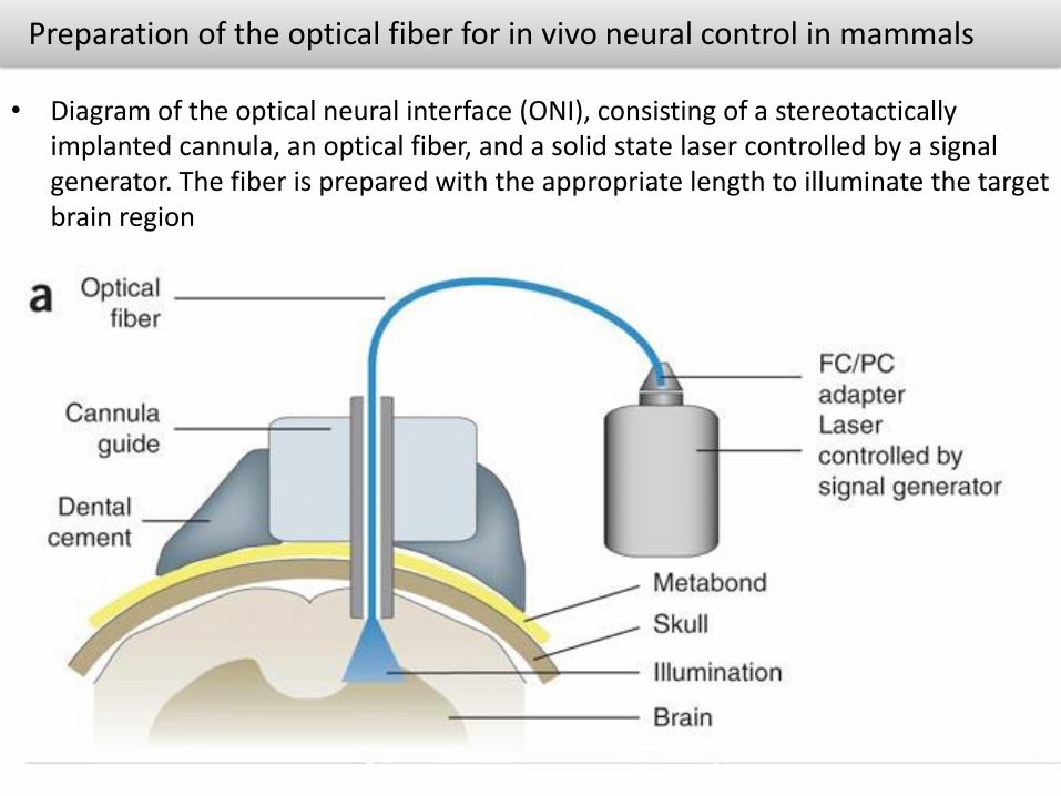
• Diagram of the optical neural interface (ONI), consisting of a stereotacticallyimplanted cannula, an optical fiber, and a solid state laser controlled by a signal generator. The fiber is prepared with the appropriate length to illuminate the target brain region

Preparation of the optical fiber for in vivo neural control in mammals

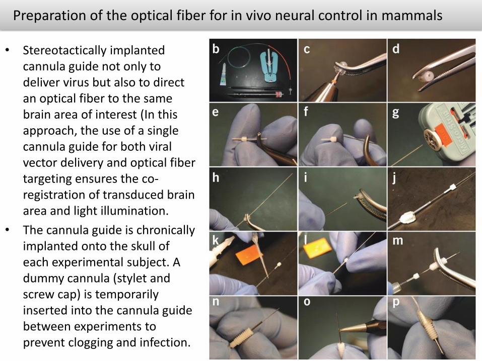
• Stereotactically implanted cannula guide not only to deliver virus but also to direct an optical fiber to the same brain area of interest (In this approach, the use of a single cannula guide for both viral vector delivery and optical fibertargeting ensures the co-registration of transduced brain area and light illumination.

• The cannula guide is chronically implanted onto the skull of each experimental subject. A dummy cannula (stylet and screw cap) is temporarily inserted into the cannula guide between experiments to prevent clogging and infection.

How do you express opsins in neurons?

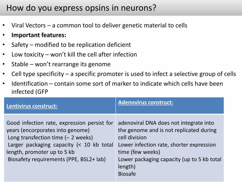
• Viral Vectors – a common tool to deliver genetic material to cells

• Important features:

• Safety – modified to be replication deficient

• Low toxicity – won’t kill the cell after infection

• Stable – won’t rearrange its genome

• Cell type specificity – a specific promoter is used to infect a selective group of cells

• Identification – contain some sort of marker to indicate which cells have been infected (GFP

Lentivirus construct:Adenovirus construct:

Good infection rate, expression persist foryears (encorporates into genome)Long transfection time ( 2 weeks)Larger packaging capacity (< 10 kb total

length, promoter up to 5 kbBiosafety requirements (PPE, BSL2+ lab)

adenoviral DNA does not integrate into the genome and is not replicated during cell divisionLower infection rate, shorter expression time (few weeks)Lower packaging capacity (up to 5 kb total length)Biosafe

Lentivirus Opsin construct

Example:

Promoter = hypocretin promoter (3.086 kb)

Fluorophore = mCherry (red)

Opsin = ChR2

Rapid on/off, precise activation of neurons on the millisecond timescale

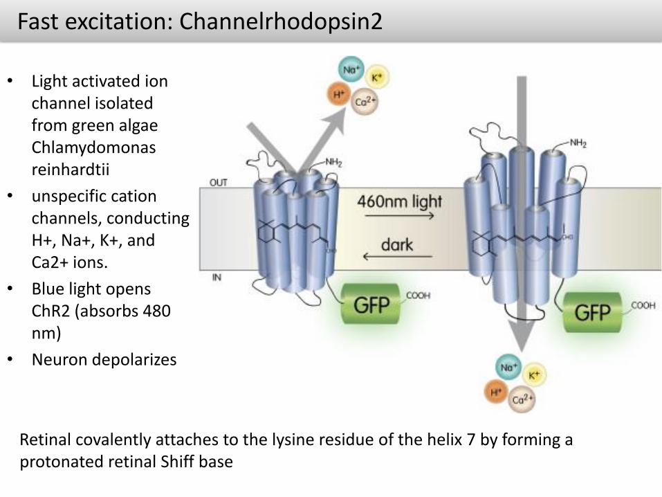
Fast excitation: Channelrhodopsin2

• Light activated ion channel isolated from green algae Chlamydomonasreinhardtii

• unspecific cationchannels, conducting H+, Na+, K+, and Ca2+ ions.

• Blue light opens ChR2 (absorbs 480 nm)

• Neuron depolarizes

Retinal covalently attaches to the lysine residue of the helix 7 by forming a protonated retinal Shiff base

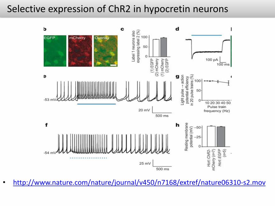
Selective expression of ChR2 in hypocretin neurons

• http://www.nature.com/nature/journal/v450/n7168/extref/nature06310-s2.mov

Bistable opsins/Step Function Opsins

• Mutate ChR to significantly prolong photocycle.

• Conductance of wildtype ChR2 deactivates ~10 ms upon light sessation.

• Mutations to ChR change the time constants of deactivation from 2, 42 to ~100 s (can stay on for long periods of time)

• SFOs can be switched on and off with blue and green light pulses, respectively

• effectively responsive to light at orders of magnitude lower intensity than wild-type channelrhodopsins

Useful for many long–time scale, neuromodulatory, developmental

chemical cofactor independence in mammalian brains. (ie not activating GPCRs – can maintain selectivity

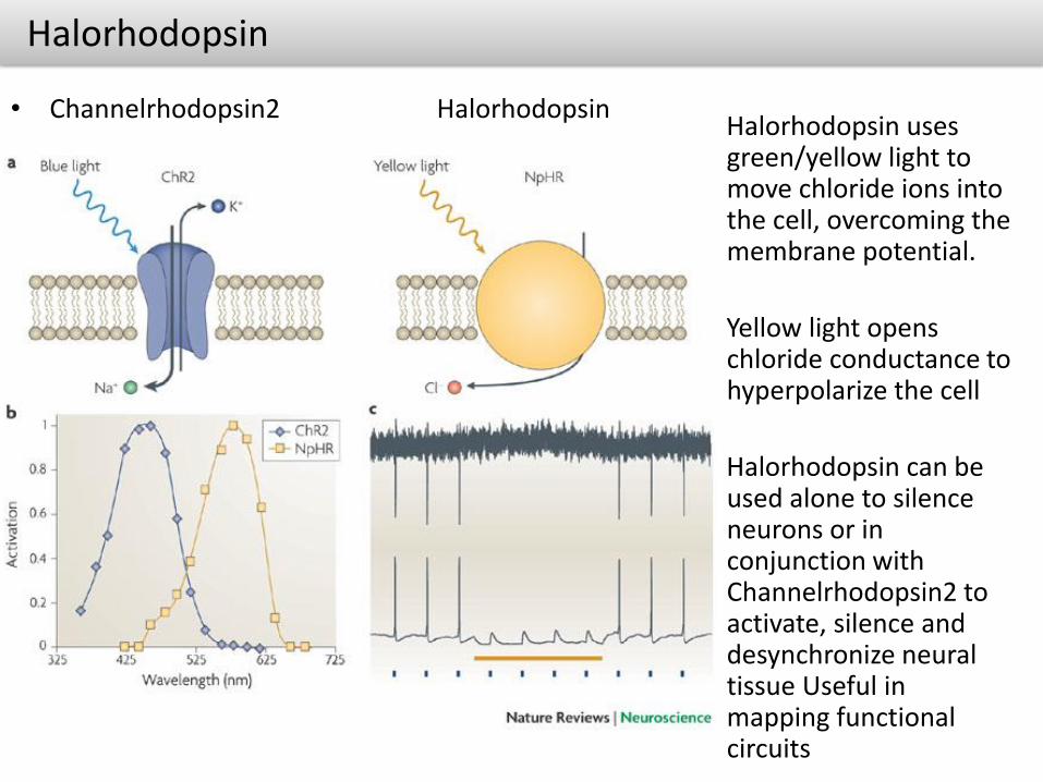
Halorhodopsin

• Channelrhodopsin2 HalorhodopsinHalorhodopsin uses green/yellow light to move chloride ions into the cell, overcoming the membrane potential.

Yellow light opens chloride conductance to hyperpolarize the cell

Halorhodopsin can be used alone to silence neurons or in conjunction with Channelrhodopsin2 to activate, silence and desynchronize neural tissue Useful in mapping functional circuits

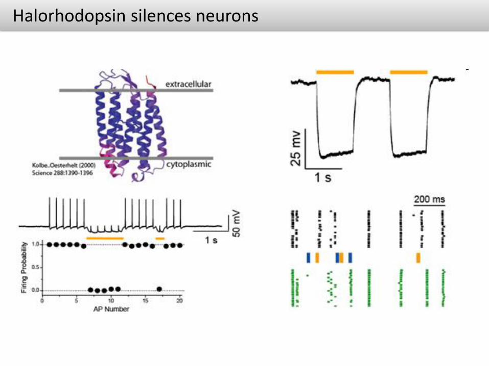
Halorhodopsin silences neurons

Light stimulation, intracellular signalling and regulation of function in neural networks

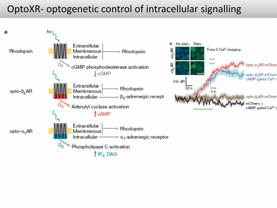
OptoXR- optogenetic control of intracellular signalling

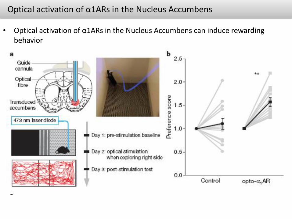
Optical activation of α1ARs in the Nucleus Accumbens

• Optical activation of α1ARs in the Nucleus Accumbens can induce rewarding behavior

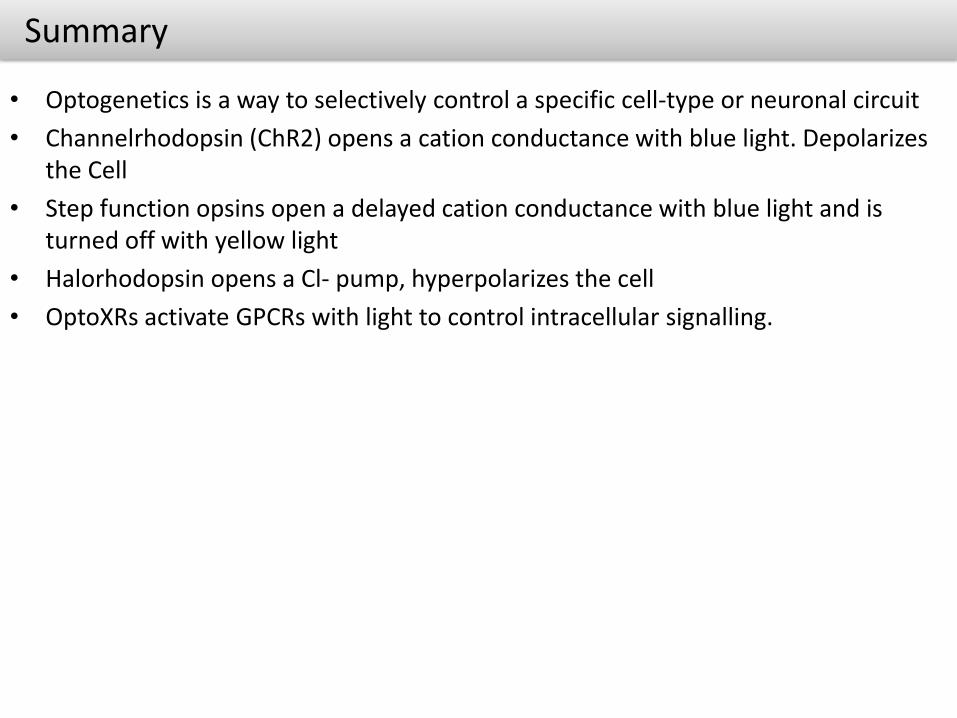
Summary

• Optogenetics is a way to selectively control a specific cell-type or neuronal circuit

• Channelrhodopsin (ChR2) opens a cation conductance with blue light. Depolarizes the Cell

• Step function opsins open a delayed cation conductance with blue light and is turned off with yellow light

• Halorhodopsin opens a Cl- pump, hyperpolarizes the cell

• OptoXRs activate GPCRs with light to control intracellular signalling.

Recent literature

• Inhibition of inhibition in visual cortex: the logic of connections between molecularly distinct interneurons

• Distinct behavioural and network correlates of two interneuron types in prefrontal cortex

• Gain control by layer six in cortical circuits of vision

• Distinct extended amygdala circuits for divergent motivational states

• Rapid regulation of depression-related behaviours by control of midbrain dopamine neurons

• Input-specific control of reward and aversion in the ventral tegmental area

• Functional identification of an aggression locus in the mouse hypothalamus

• Deconstruction of a neural circuit for hunger

• Creating a false memory in the hippocampus

Why Single Particle Tracking?

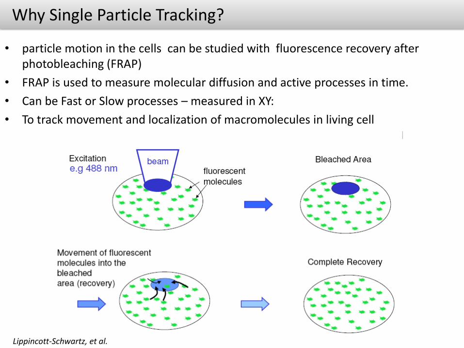
• particle motion in the cells can be studied with fluorescence recovery after photobleaching (FRAP)

• FRAP is used to measure molecular diffusion and active processes in time.

• Can be Fast or Slow processes – measured in XY:

• To track movement and localization of macromolecules in living cell

Lippincott-Schwartz, et al.

Why Single Particle Tracking?

• FRAP: Mode of operation

• 1. Determination of pre-bleach levels

• 2. Photobleaching (short excitation pulse) of selected cells / areas.

• 3. Recovery: diffusion of unbleached molecules into the bleached area and increase of fluorescence intensity. Record the time course of fluorescence recovery at various time intervals, using a light level sufficiently low to prevent further bleaching.

• 4. Quantification: graph shows the time course of fluorescence recovery (calculated as average percentage recovery of initial fluorescence

Calculation of recovery normalized

Each fluorophore has different photobleaching characteristics. For FRAP experiments it is important to choose a dye which bleaches minimally at low illumination power (to prevent photobleaching during image acquisition) but bleaches fast and irreversibly at highillumination power.

Why Single Particle Tracking?

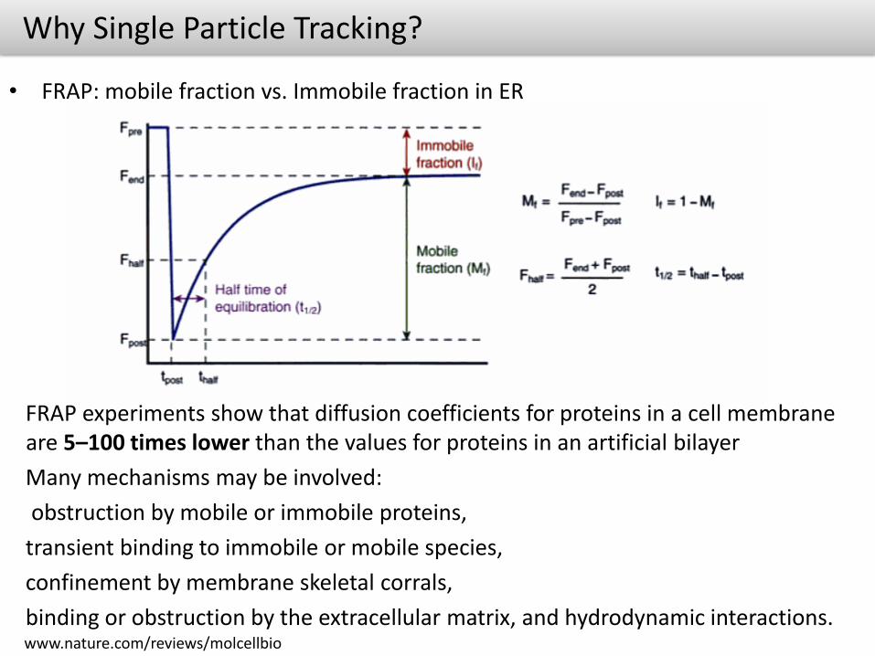
• FRAP: mobile fraction vs. Immobile fraction in ER

www.nature.com/reviews/molcellbio

FRAP experiments show that diffusion coefficients for proteins in a cell membrane are 5–100 times lower than the values for proteins in an artificial bilayer

Many mechanisms may be involved:

obstruction by mobile or immobile proteins,

transient binding to immobile or mobile species,

confinement by membrane skeletal corrals,

binding or obstruction by the extracellular matrix, and hydrodynamic interactions.

Why Single Particle Tracking?

• These mechanisms have been difficult to sort out,

• of them may occur simultaneously, and their relative importance may depend on the protein and the cell type

• Second, a significant fraction of protein and lipid is immobile on the time scale of a FRAP experiment. For artificial bilayers and rhodopsin in the rod outer segment, recovery is close to 100%, but in the plasma membrane, recovery is typically 25% to 80%

• Third, in FRAP experiments, the distribution of observed diffusion coefficients D is much broader than expected from experimental error . Values of D vary around twofold among different points on a single cell, and tenfold among cells This suggests significant heterogeneity in the membrane, a view supported by other evidence

• The increased resolution of SPT ought to make it possible to understand the FRAP immobile fraction.

Single particle tracking-SPT

• In single particle tracking SPT, computer ‘enhanced video-microscopy is used to track the motion of proteins or lipids on the cell surface .

• Individual molecules are observed with a typical spatial resolution of tens of nanometers and typical time resolution of tens of milliseconds .

• The technique is addressing following questions

• 1. How do particle move on the cell surface ? To what extent does the motion of various particles deviates from pure diffusion ? How is that motion controlled and what is it function ?

• 2. How is the cell surface organized ? To what extent membranes deviate from the fluid mosaic model? Is a fractal time model a useful description of the cell surface ? How are structures on the cell surface assembled ? Does compertmentationprevent crosstalk of receptors What regional or global control over cell membrane dynamics exists?

• What are the effects of heterogeneous motion in a heterogeneous environment on kinetics and equilibrium?

Capabilities of Single particle tracking-SPT

• The spatial resolution is approximately two orders of magnitude higher than FRAP, so that with sufficient time resolution motion in small domains can be characterized.

• The time resolution is similar to FRAP, so the minimum detectable diffusion coefficient is lowered by approximately two orders of magnitude.

• FRAP averages over hundreds or thousands of diffusing molecules, but SPT measures individual trajectories. Thus, different subpopulations indistinguishable by FRAP can be resolved.

• SPT provides the ultimate specificity in measurement of motion of membrane components, particularly if the individual particle tracked could be characterized in terms of, for example, its phosphorylation state.

• How do individual molecules move in the cell?

Modes of Motion

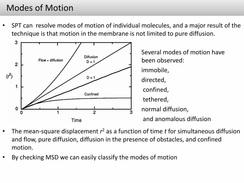
• SPT can resolve modes of motion of individual molecules, and a major result of the technique is that motion in the membrane is not limited to pure diffusion.

• The mean-square displacement r2 as a function of time t for simultaneous diffusion and flow, pure diffusion, diffusion in the presence of obstacles, and confined motion.

• By checking MSD we can easily classify the modes of motion

Several modes of motion have been observed:

immobile,

directed,

confined,

tethered,

normal diffusion,

and anomalous diffusion

Random walks, diffusion

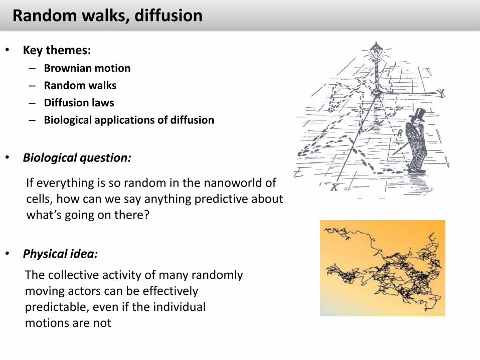
• Key themes:

– Brownian motion

– Random walks

– Diffusion laws

– Biological applications of diffusion

• Biological question:

• Physical idea:

If everything is so random in the nanoworld of cells, how can we say anything predictive about what’s going on there?

The collective activity of many randomly moving actors can be effectivelypredictable, even if the individual motions are not

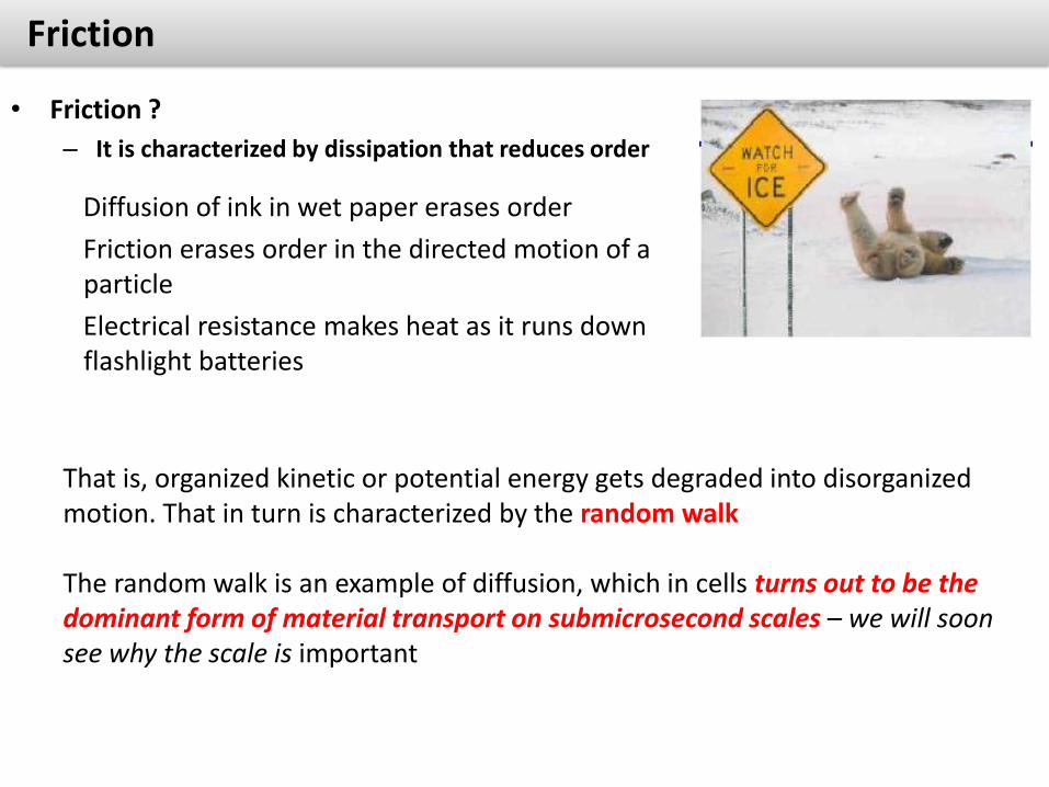
Friction

Diffusion of ink in wet paper erases order

Friction erases order in the directed motion of a particle

Electrical resistance makes heat as it runs down flashlight batteries

• Friction ?

– It is characterized by dissipation that reduces order

That is, organized kinetic or potential energy gets degraded into disorganized motion. That in turn is characterized by the random walk

The random walk is an example of diffusion, which in cells turns out to be the dominant form of material transport on submicrosecond scales – we will soon see why the scale is important

Brownian motion

Tiny solvent molecules interacting with the colloid through collisions

Colloid mass much larger than the mass of solvent molecules

While the effect of each single collision is almost negligible, the large number of them gives rise to macroscopic observable motion

Brownian motion is thus driven by thermal energy

Robert Brown: observed in 1827

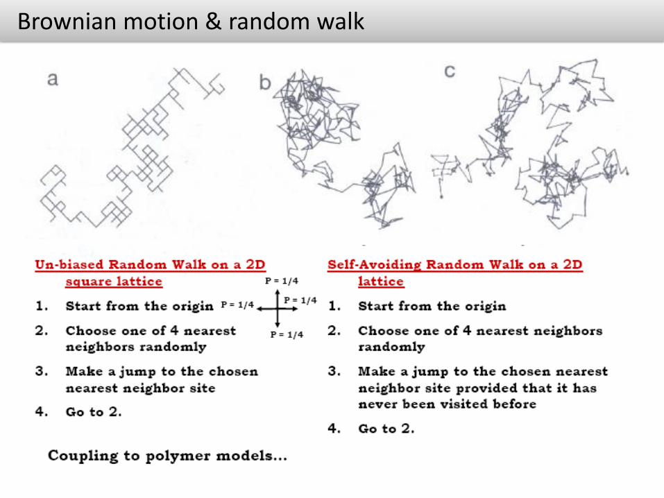
Brownian motion & random walk

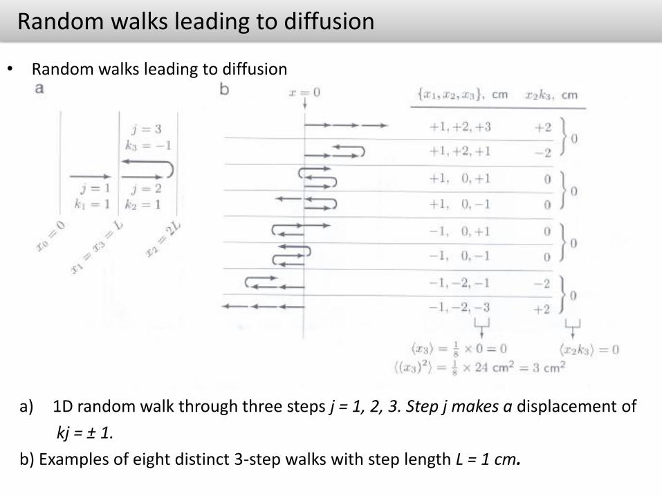
Random walks leading to diffusion

• Random walks leading to diffusion

a) 1D random walk through three steps j = 1, 2, 3. Step j makes a displacement of

kj = ± 1.

b) Examples of eight distinct 3-step walks with step length L = 1 cm.

Random walk leading to diffusion

• Random walk in d = 1 dimension:

• For simplicity, consider a random walk in 1D. Position after n steps xn,

• x0 = 0, δ is constant, and jumps take place with an interval of τ .

Clearly < xn > = 0 for all n .

The second moments, however, yield

1

2 1

1N N

x

x x

x x

2 2

1

2 2 2 2

2 1 1

2 2

2

N

x

x x x

x N

Here the discrete step number N relates to time t, thus we have

2 2

1( )t

x t

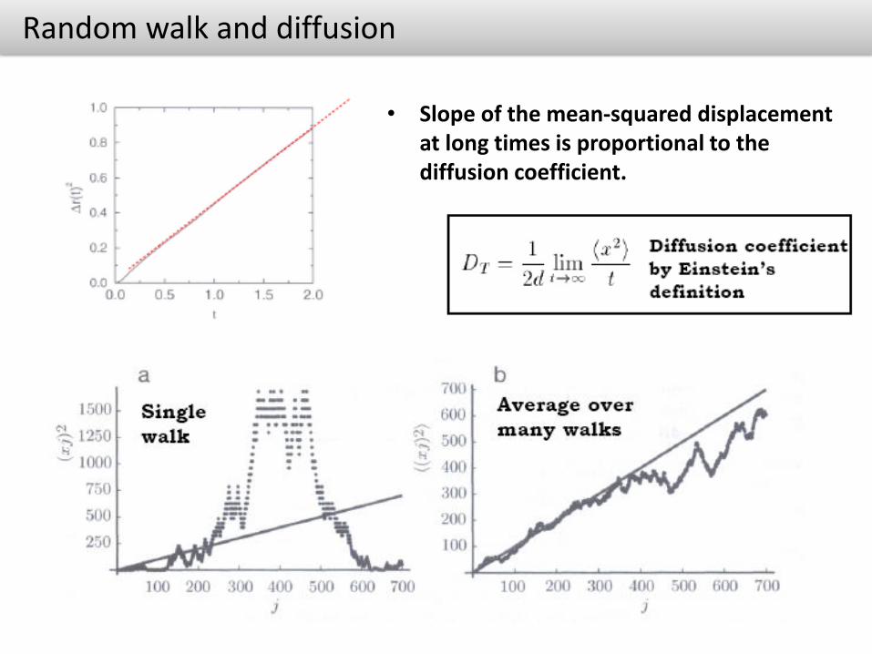
Random walk and diffusion

• Slope of the mean-squared displacement at long times is proportional to the diffusion coefficient.

Friction coupled to diffusion

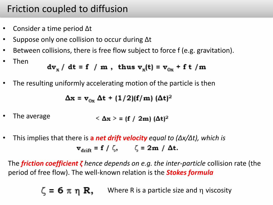
• Consider a time period Δt

• Suppose only one collision to occur during Δt

• Between collisions, there is free flow subject to force f (e.g. gravitation).

• Then

• The resulting uniformly accelerating motion of the particle is then

• The average

• This implies that there is a net drift velocity equal to (Δx/Δt), which is

The friction coefficient ζ hence depends on e.g. the inter-particle collision rate (the period of free flow). The well-known relation is the Stokes formula

Where R is a particle size and h viscosity

Friction coupled to diffusion

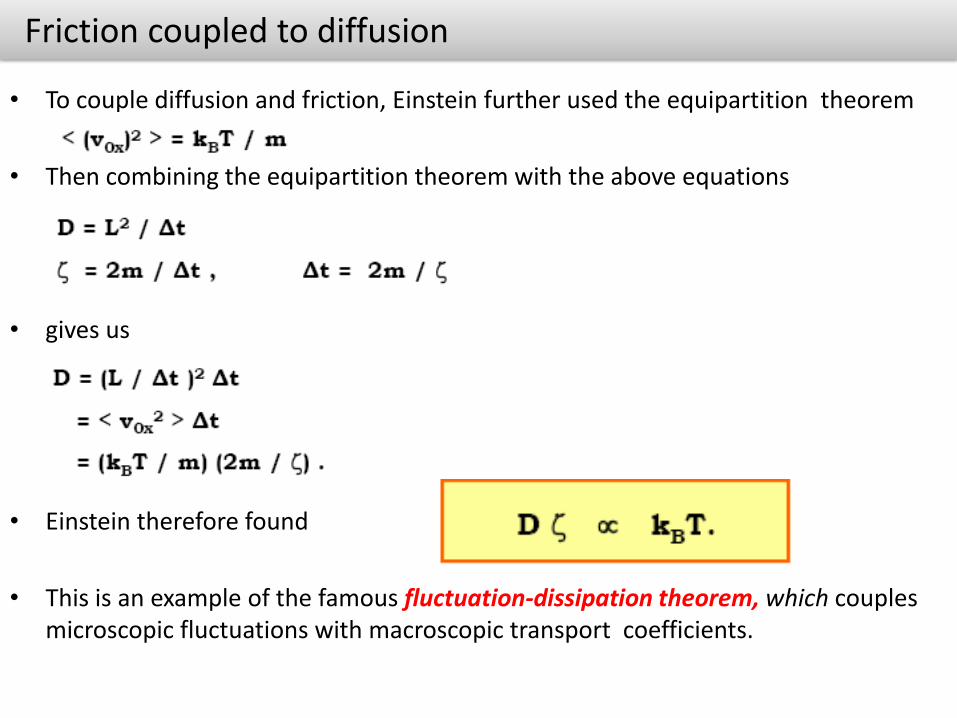
• To couple diffusion and friction, Einstein further used the equipartition theorem

• Then combining the equipartition theorem with the above equations

• gives us

• Einstein therefore found

• This is an example of the famous fluctuation-dissipation theorem, which couples microscopic fluctuations with macroscopic transport coefficients.

Friction & Diffusion: Langevin equation

• Brownian diffusion for a colloidal particle, using the Langevin equation

Diffusion equation

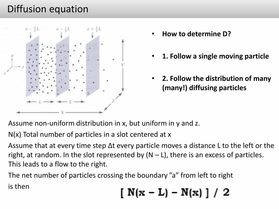
• How to determine D?

• 1. Follow a single moving particle

• 2. Follow the distribution of many (many!) diffusing particles

Assume non-uniform distribution in x, but uniform in y and z.

N(x) Total number of particles in a slot centered at x

Assume that at every time step Δt every particle moves a distance L to the left or the right, at random. In the slot represented by (N – L), there is an excess of particles. This leads to a flow to the right.

The net number of particles crossing the boundary ”a” from left to right

is then

Diffusion equation

• Considering L to be very small, we get

• Dividing N(x) by the volume of the slice

• (V = XYZ), we are given the number density of particles, c(x).

• Then the flux (number of particles crossing ”a” (from left to right) per unit area per unit time) is

This corresponds to Fick’s first law

The flux is hence driven by the density gradient

Diffusion equation

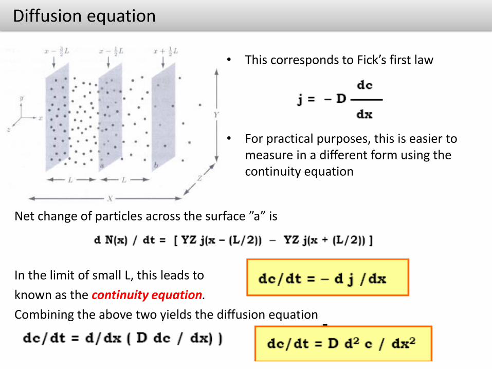
• This corresponds to Fick’s first law

• For practical purposes, this is easier to measure in a different form using the continuity equation

Net change of particles across the surface ”a” is

In the limit of small L, this leads to

known as the continuity equation.

Combining the above two yields the diffusion equation

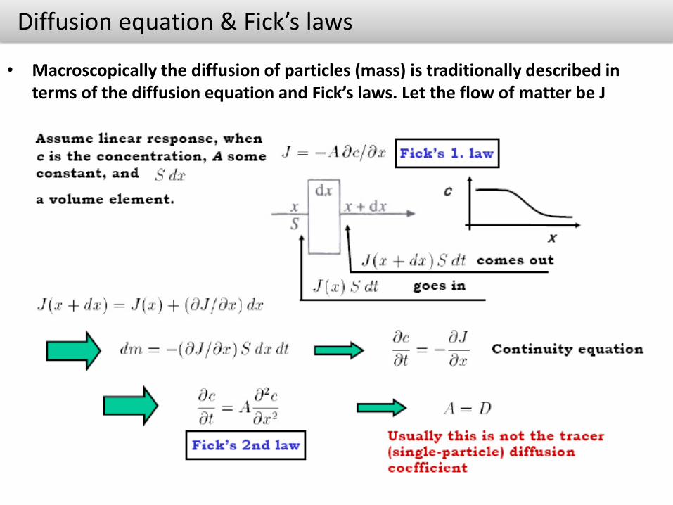
Diffusion equation & Fick’s laws

• Macroscopically the diffusion of particles (mass) is traditionally described in terms of the diffusion equation and Fick’s laws. Let the flow of matter be J

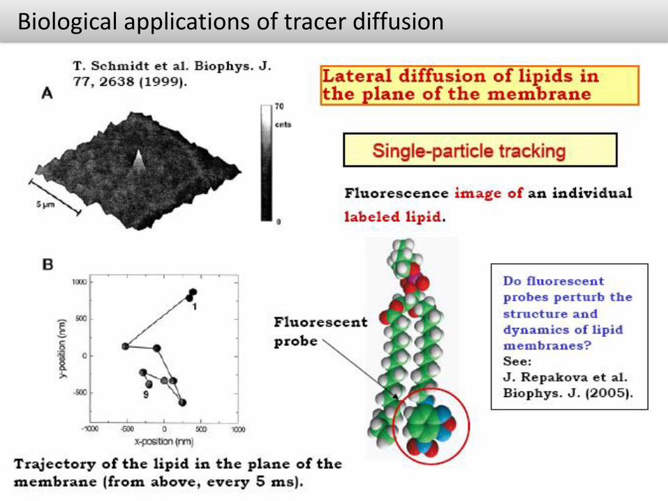
Biological applications of tracer diffusion

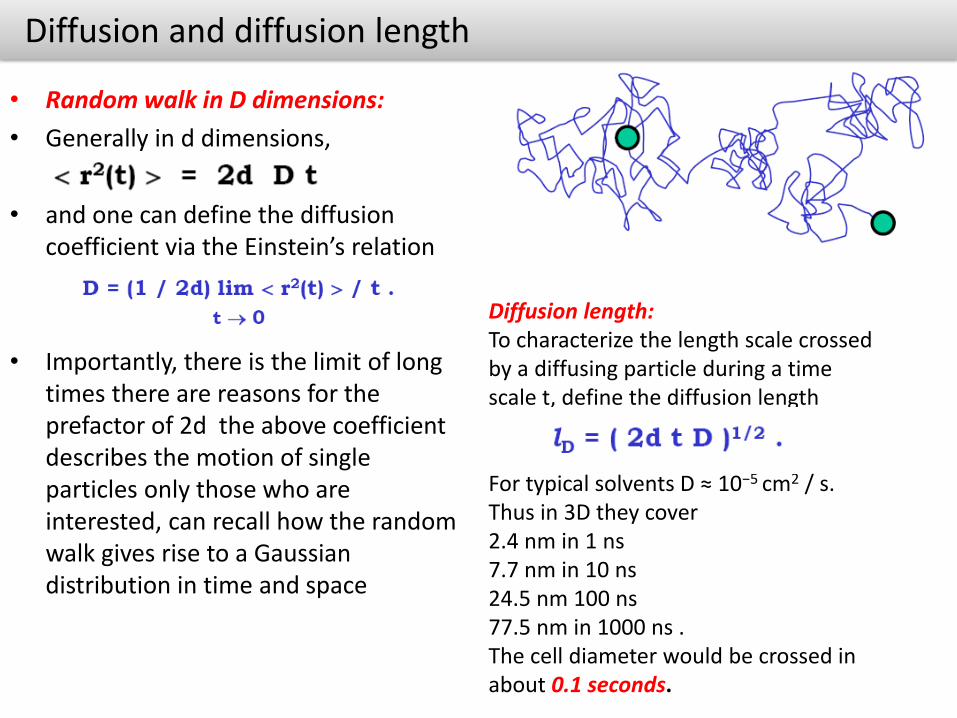
Diffusion and diffusion length

• Random walk in D dimensions:

• Generally in d dimensions,

• and one can define the diffusion coefficient via the Einstein’s relation

• Importantly, there is the limit of long times there are reasons for the prefactor of 2d the above coefficient describes the motion of single particles only those who are interested, can recall how the random walk gives rise to a Gaussian distribution in time and space

Diffusion length:To characterize the length scale crossedby a diffusing particle during a timescale t, define the diffusion length

For typical solvents D ≈ 10−5 cm2 / s.Thus in 3D they cover2.4 nm in 1 ns7.7 nm in 10 ns24.5 nm 100 ns77.5 nm in 1000 ns .The cell diameter would be crossed inabout 0.1 seconds.

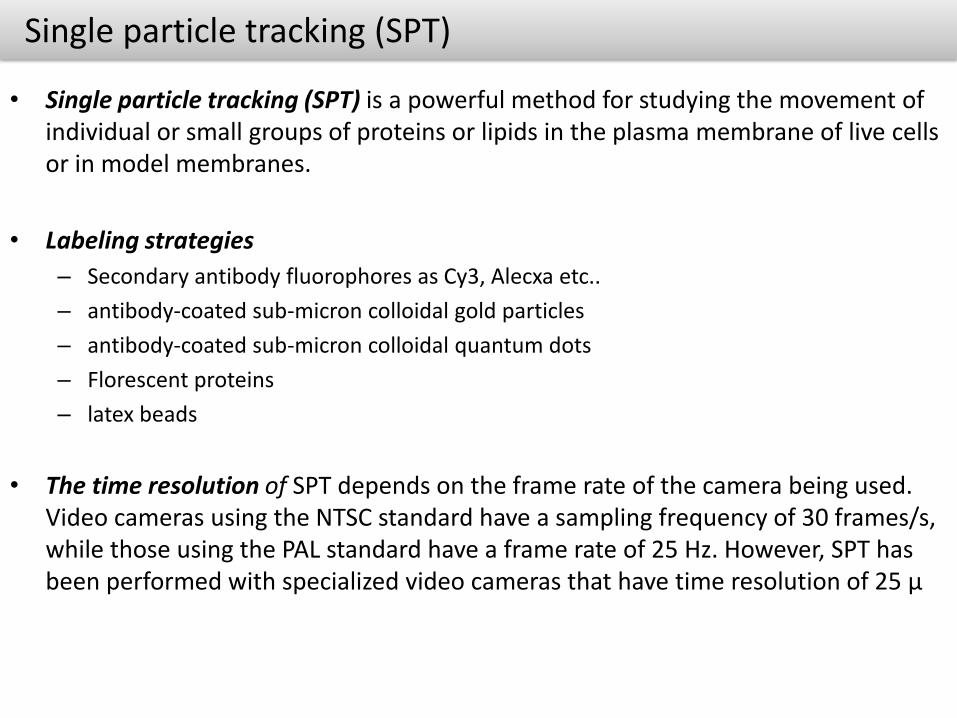
Single particle tracking (SPT)

• Single particle tracking (SPT) is a powerful method for studying the movement of individual or small groups of proteins or lipids in the plasma membrane of live cells or in model membranes.

• Labeling strategies

– Secondary antibody fluorophores as Cy3, Alecxa etc..

– antibody-coated sub-micron colloidal gold particles

– antibody-coated sub-micron colloidal quantum dots

– Florescent proteins

– latex beads

• The time resolution of SPT depends on the frame rate of the camera being used. Video cameras using the NTSC standard have a sampling frequency of 30 frames/s, while those using the PAL standard have a frame rate of 25 Hz. However, SPT has been performed with specialized video cameras that have time resolution of 25 μ

Labelling bottelnecks

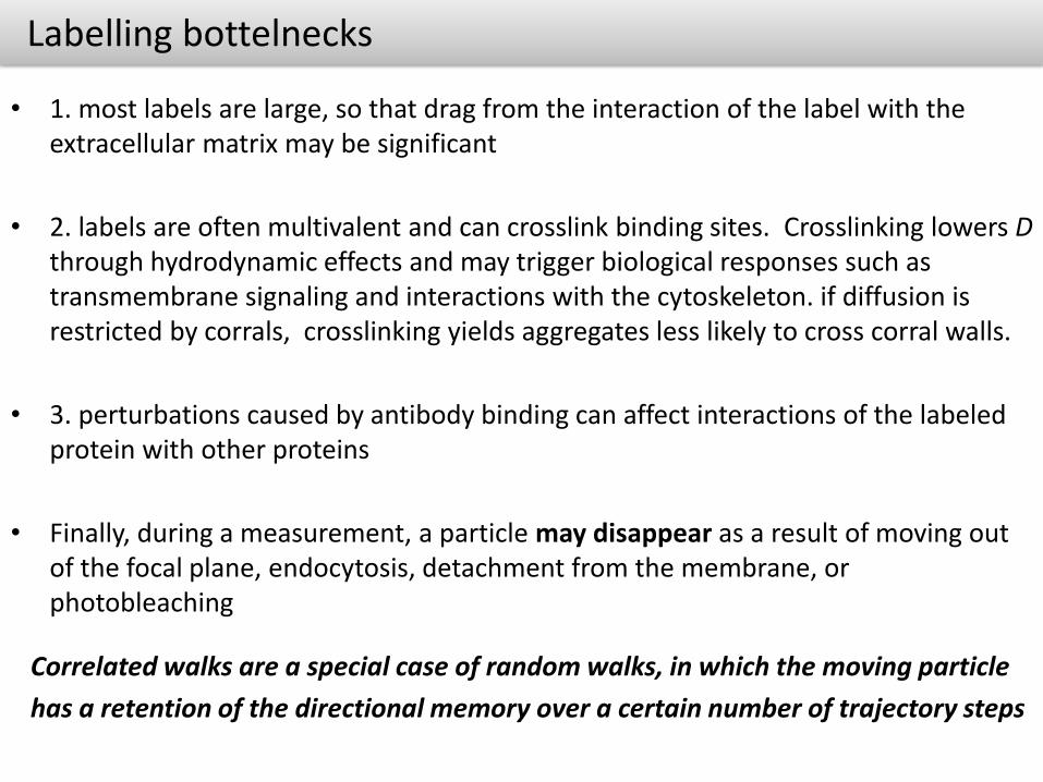
• 1. most labels are large, so that drag from the interaction of the label with the extracellular matrix may be significant

• 2. labels are often multivalent and can crosslink binding sites. Crosslinking lowers Dthrough hydrodynamic effects and may trigger biological responses such as transmembrane signaling and interactions with the cytoskeleton. if diffusion is restricted by corrals, crosslinking yields aggregates less likely to cross corral walls.

• 3. perturbations caused by antibody binding can affect interactions of the labeled protein with other proteins

• Finally, during a measurement, a particle may disappear as a result of moving out of the focal plane, endocytosis, detachment from the membrane, or photobleaching

Correlated walks are a special case of random walks, in which the moving particle

has a retention of the directional memory over a certain number of trajectory steps

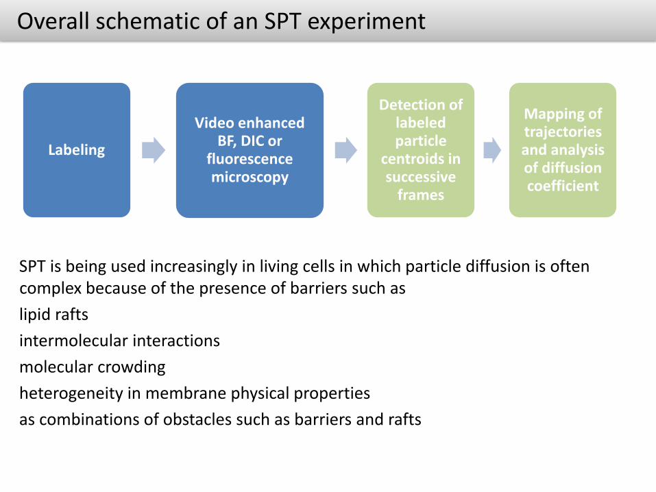
Overall schematic of an SPT experiment

Labeling

Video enhanced BF, DIC or

fluorescence microscopy

Detection of labeled particle

centroids in successive

frames

Mapping of trajectories and analysis of diffusion coefficient

SPT is being used increasingly in living cells in which particle diffusion is often complex because of the presence of barriers such as

lipid rafts

intermolecular interactions

molecular crowding

heterogeneity in membrane physical properties

as combinations of obstacles such as barriers and rafts

SPT trajectory classification

• How to sort out trajectories !

• Be careful do controls for data analysis using a pure random walk as a reference. The minimum test for a classification algorithm is to try it on pure random walks of the appropriate number of time steps.

• The analytical forms of the curves of MSD versus time for the different modes of motion form the basis of various classification methods.

If a <1 the motion is classified as subdiffuison . rc is corral size and A1 and A2 are constants determined by corral geometry

SPT trajectory classification

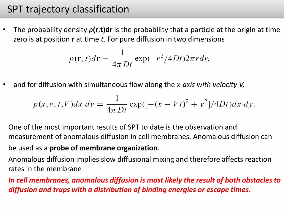
• The probability density p(r,t)dr is the probability that a particle at the origin at time zero is at position r at time t. For pure diffusion in two dimensions

• and for diffusion with simultaneous flow along the x-axis with velocity V,

One of the most important results of SPT to date is the observation and measurement of anomalous diffusion in cell membranes. Anomalous diffusion can

be used as a probe of membrane organization.

Anomalous diffusion implies slow diffusional mixing and therefore affects reaction rates in the membrane

In cell membranes, anomalous diffusion is most likely the result of both obstacles to diffusion and traps with a distribution of binding energies or escape times.

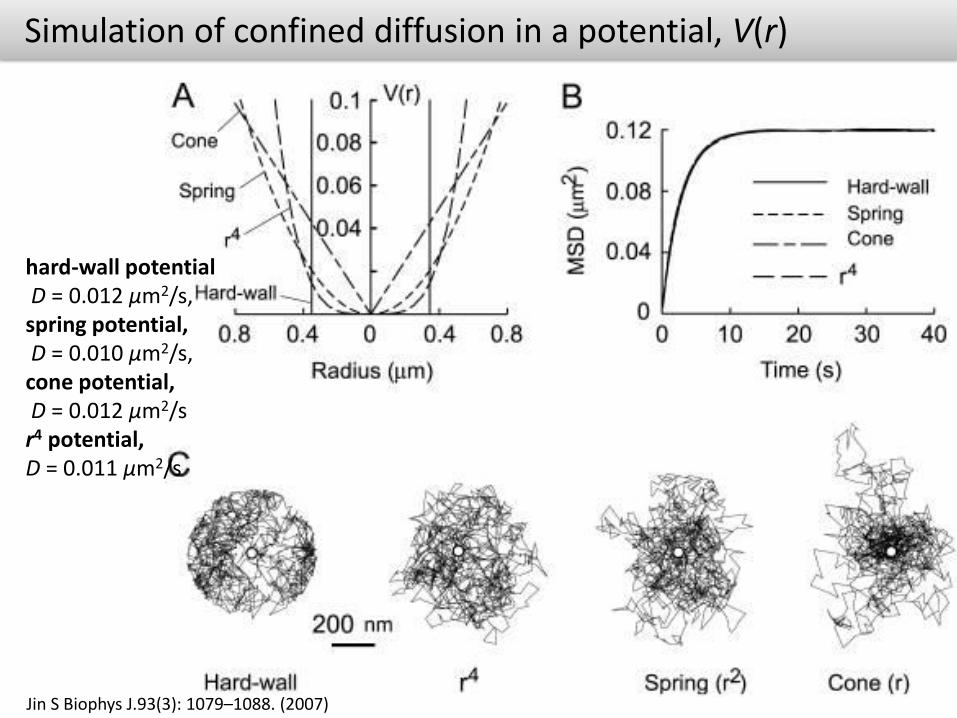
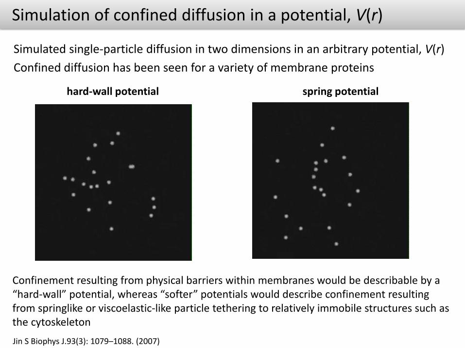
Simulation of confined diffusion in a potential, V(r)

Jin S Biophys J.93(3): 1079–1088. (2007)

hard-wall potentialD = 0.012 μm2/s,

spring potential,D = 0.010 μm2/s,

cone potential,D = 0.012 μm2/s

r4 potential, D = 0.011 μm2/s

Simulation of confined diffusion in a potential, V(r)

Jin S Biophys J.93(3): 1079–1088. (2007)

Simulated single-particle diffusion in two dimensions in an arbitrary potential, V(r)

Confined diffusion has been seen for a variety of membrane proteins

hard-wall potential spring potential

Confinement resulting from physical barriers within membranes would be describable by a “hard-wall” potential, whereas “softer” potentials would describe confinement resulting from springlike or viscoelastic-like particle tethering to relatively immobile structures such as the cytoskeleton

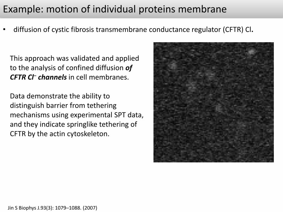
Example: motion of individual proteins membrane

• diffusion of cystic fibrosis transmembrane conductance regulator (CFTR) Cl.

Jin S Biophys J.93(3): 1079–1088. (2007)

This approach was validated and applied to the analysis of confined diffusion of CFTR Cl− channels in cell membranes.

Data demonstrate the ability to distinguish barrier from tethering mechanisms using experimental SPT data, and they indicate springlike tethering of CFTR by the actin cytoskeleton.

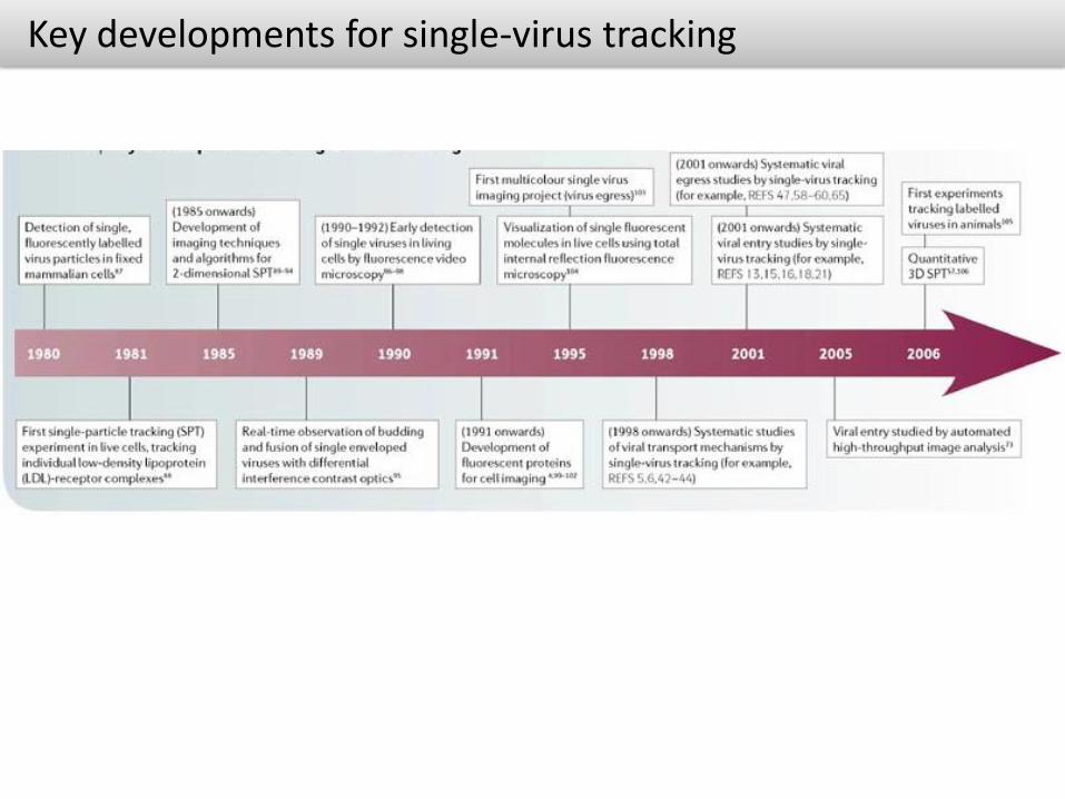
Key developments for single-virus tracking

Strategies for labelling various viral components

• Two general strategies exist for labelling viruses: the fusion of a target viral protein

• with a fluorescent protein (FP), or direct chemical labelling with small dye molecules.

• FP advantages

– broad range of colours,

– pH sensitive

– photo-switchable

• FP disadvantages

– Labelling occurs during

– virus replication in host cells

– Requires several FP proteins

• CL advantages

– labelling can be at different time-points during the viral life cycle

– covalently attached or non-covalently associated with the target protein

• CL disadvantages

– Cant use antibodies block the function of viral proteins after binding.

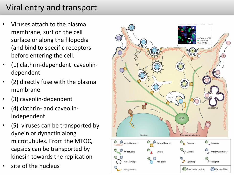
Viral entry and transport

• Viruses attach to the plasma membrane, surf on the cell surface or along the filopodia(and bind to specific receptors before entering the cell.

• (1) clathrin-dependent caveolin-dependent

• (2) directly fuse with the plasma membrane

• (3) caveolin-dependent

• (4) clathrin- and caveolin-independent

• (5) viruses can be transported by dynein or dynactin along microtubules. From the MTOC, capsids can be transported by kinesin towards the replication

• site of the nucleus

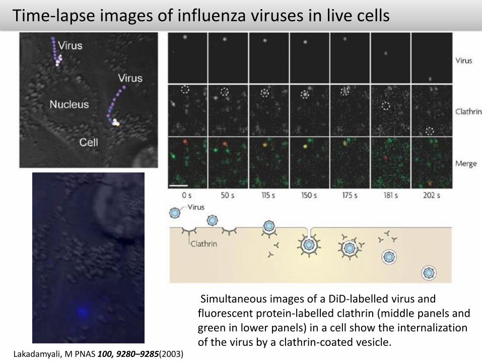
Time-lapse images of influenza viruses in live cells

Lakadamyali, M PNAS 100, 9280–9285(2003)

Simultaneous images of a DiD-labelled virus and fluorescent protein-labelled clathrin (middle panels and green in lower panels) in a cell show the internalization of the virus by a clathrin-coated vesicle.

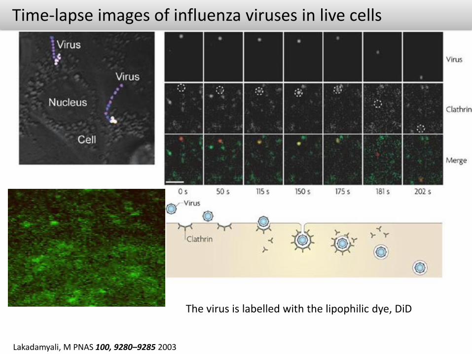
Time-lapse images of influenza viruses in live cells

Lakadamyali, M PNAS 100, 9280–9285 2003

The virus is labelled with the lipophilic dye, DiD

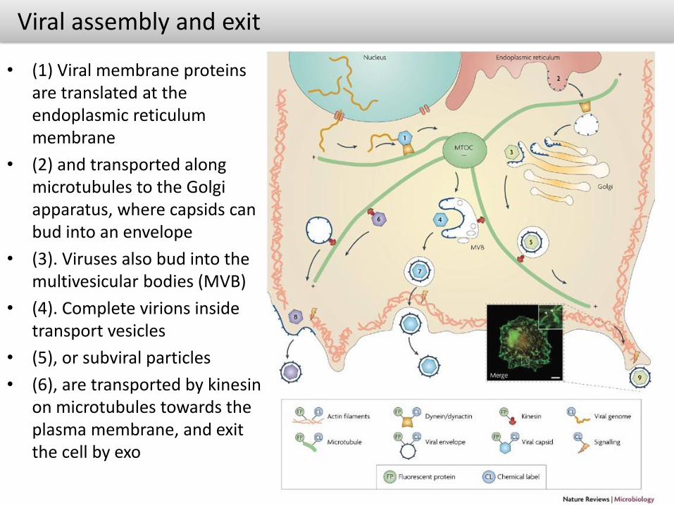
Viral assembly and exit

• (1) Viral membrane proteins are translated at the endoplasmic reticulum membrane

• (2) and transported along microtubules to the Golgi apparatus, where capsids can bud into an envelope

• (3). Viruses also bud into the multivesicular bodies (MVB)

• (4). Complete virions inside transport vesicles

• (5), or subviral particles

• (6), are transported by kinesinon microtubules towards the plasma membrane, and exit the cell by exo

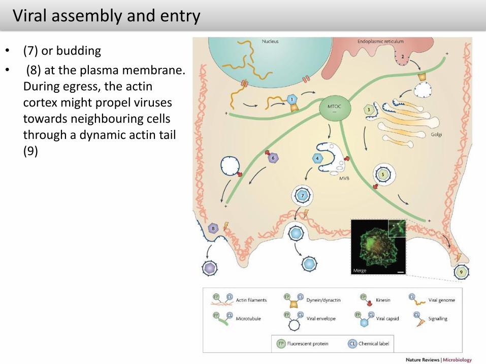
Viral assembly and entry

• (7) or budding

• (8) at the plasma membrane. During egress, the actincortex might propel viruses towards neighbouring cells through a dynamic actin tail (9)

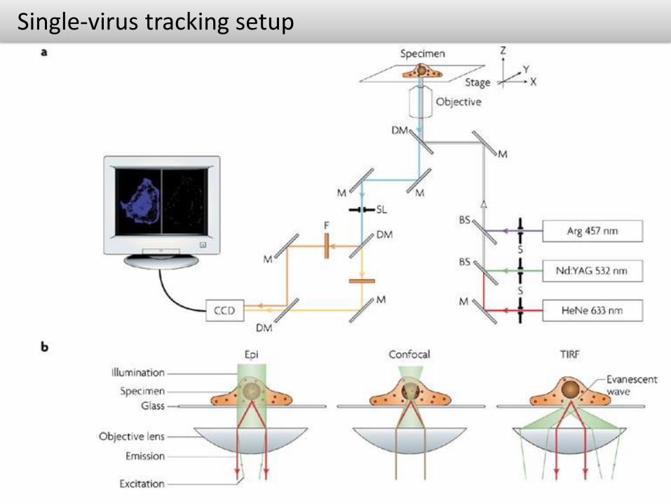
Single-virus tracking setup

Kinetics of clathrin-mediated endocytosis

Clathrin is a trimer composed of three heavy chains and three light chains, each monomer projecting outwards like a leg; this three-legged structure is known

Particle Tracking -

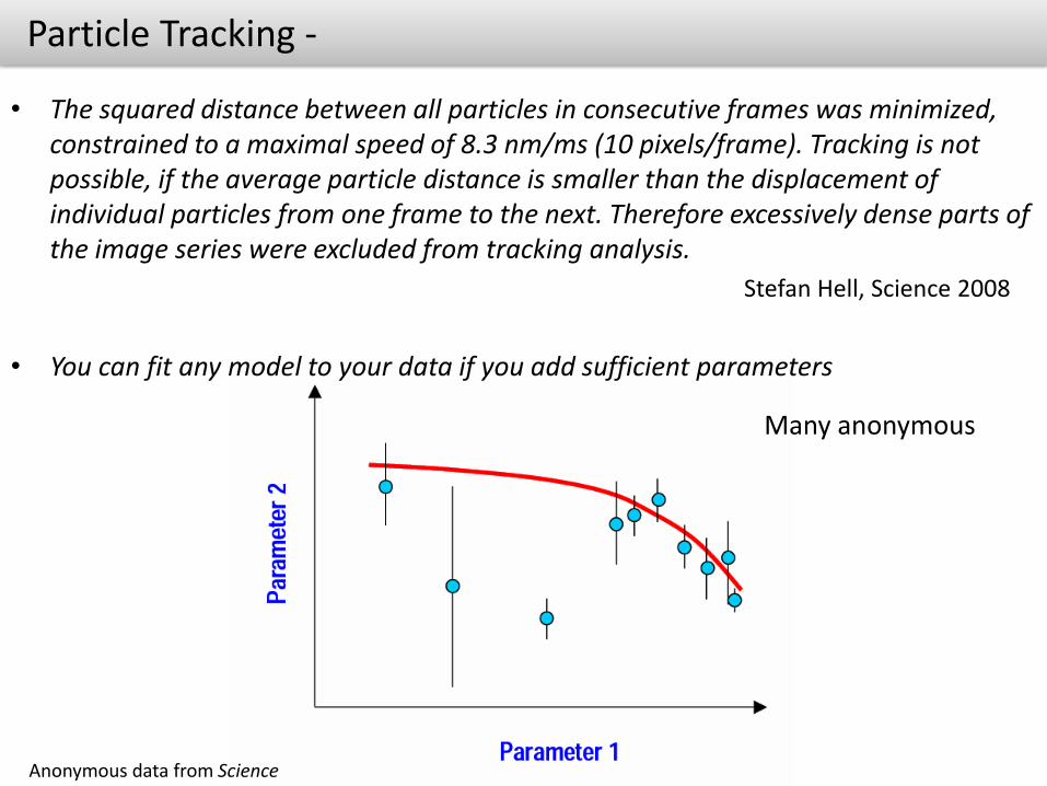
• The squared distance between all particles in consecutive frames was minimized, constrained to a maximal speed of 8.3 nm/ms (10 pixels/frame). Tracking is not possible, if the average particle distance is smaller than the displacement of individual particles from one frame to the next. Therefore excessively dense parts of the image series were excluded from tracking analysis.

Stefan Hell, Science 2008

• You can fit any model to your data if you add sufficient parameters

Anonymous data from Science

Many anonymous

SPT –algorithms challenges

• A model is valid only if it fits all experimental data within the margins of measurement uncertainty.

• If under the above conditions any two models are valid, the models are indistinguishable, i.e. equivalent.

GOOD SPT tracking algorithm has to that addresses the principal challenges of

namely high particle density

particle motion heterogeneity

temporary particle disappearance,

particle merging and splitting.

many of these challenges have been overcome by diluting the fluorescent probes, which resulted in a low particle density with almost unambiguous particle correspondence particle tracking is indeed reduced to a simple particle detection and localization problem.

Gaudenz Danuser

Gaudenz Danuser

Objectives of the good tracking algorithm

• analysis of low labeling density samples that does not allow probing of the interactions between particles . The amount of data collected per experiment is low, limiting the observation of spatially and temporally heterogeneous particle behavior and hindering the capture of infrequent event

• Even with low particle density, low signal-to-noise ratio (SNR) and probe flicker complicate the search for particle correspondence.

• Obtain a complete and accurate representation of the movement of all particles from appearance to disappearance independent of their heterogeneous images, dynamics, and neighborhood relations.

• No a priori selection of particle behaviors

• Measure as much as possible simultaneously

• DO NOT KILL DISCOVERY UPFRONT !

Additional issues: Track termination and initiation, gaps and merges

• How to avoid false continuation on another existing track?

• How to avoid false continuation on an initiating track in the next frame?

In general terms: Initiation and termination of tracks violate the constrain that every source has a target and every target has a source.

GAPS MERGE

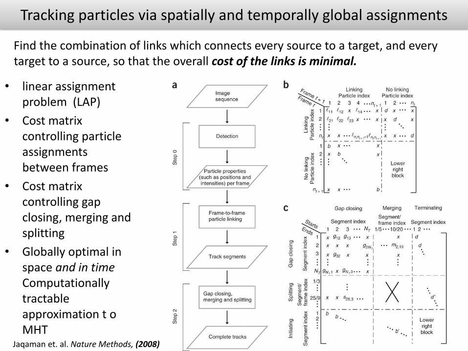
Tracking particles via spatially and temporally global assignments

• linear assignment problem (LAP)

• Cost matrix controlling particle assignments between frames

• Cost matrix controlling gap closing, merging and splitting

• Globally optimal in space and in time Computationally tractable approximation t o MHT

Jaqaman et. al. Nature Methods, (2008)

Find the combination of links which connects every source to a target, and every target to a source, so that the overall cost of the links is minimal.

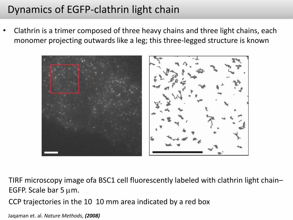
Dynamics of EGFP-clathrin light chain

• Clathrin is a trimer composed of three heavy chains and three light chains, each monomer projecting outwards like a leg; this three-legged structure is known

Jaqaman et. al. Nature Methods, (2008)

TIRF microscopy image ofa BSC1 cell fluorescently labeled with clathrin light chain–EGFP. Scale bar 5 mm.

CCP trajectories in the 10 10 mm area indicated by a red box

Dynamics of EGFP-clathrin light chain

Jaqaman et. al. Nature Methods, (2008)