g52iip, school of computer science, university of nottingham 1 edge detection and image segmentation
TRANSCRIPT

G52IIP, School of Computer Science, University of Nottingham
1
Edge Detection and Image Segmentation
G52IIP, School of Computer Science, University of Nottingham
2
Edge Detection and Image Segmentation
Detection of discontinuities
PointsLinesEdges
G52IIP, School of Computer Science, University of Nottingham
3
Edge Detection and Image Segmentation

G52IIP, School of Computer Science, University of Nottingham
4
Edge Detection and Image Segmentation
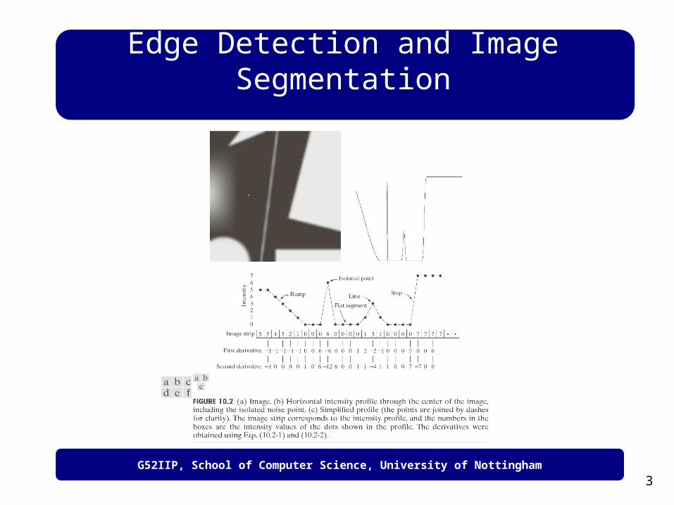
Detection of discontinuities
9
1iii zwR
Zi corresponding pixel values

G52IIP, School of Computer Science, University of Nottingham
5
Edge Detection and Image Segmentation
Point detection
TR
G52IIP, School of Computer Science, University of Nottingham
6
Edge Detection and Image Segmentation
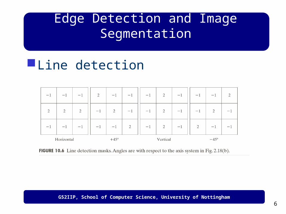
Line detection
G52IIP, School of Computer Science, University of Nottingham
7
Edge Detection and Image Segmentation
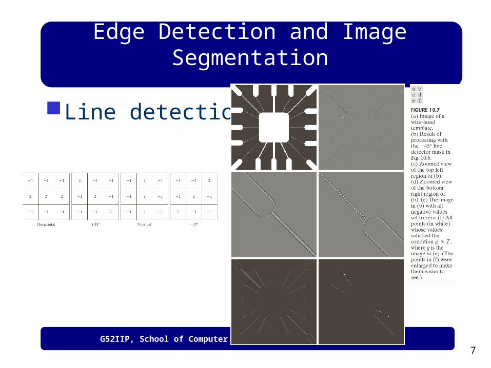
Line detection
G52IIP, School of Computer Science, University of Nottingham
8
Edge Detection and Image Segmentation
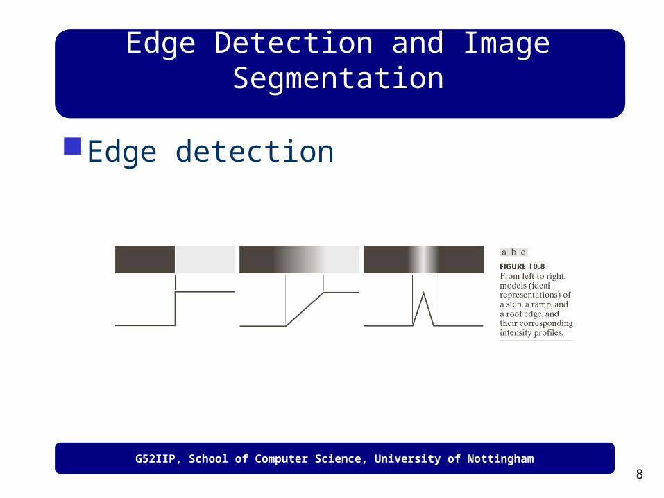
Edge detection

G52IIP, School of Computer Science, University of Nottingham
9
Edge Detection and Image Segmentation
Edge detection
G52IIP, School of Computer Science, University of Nottingham
10
Edge Detection and Image Segmentation
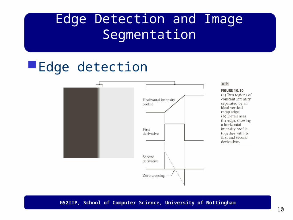
Edge detection
G52IIP, School of Computer Science, University of Nottingham
11
Edge Detection and Image Segmentation
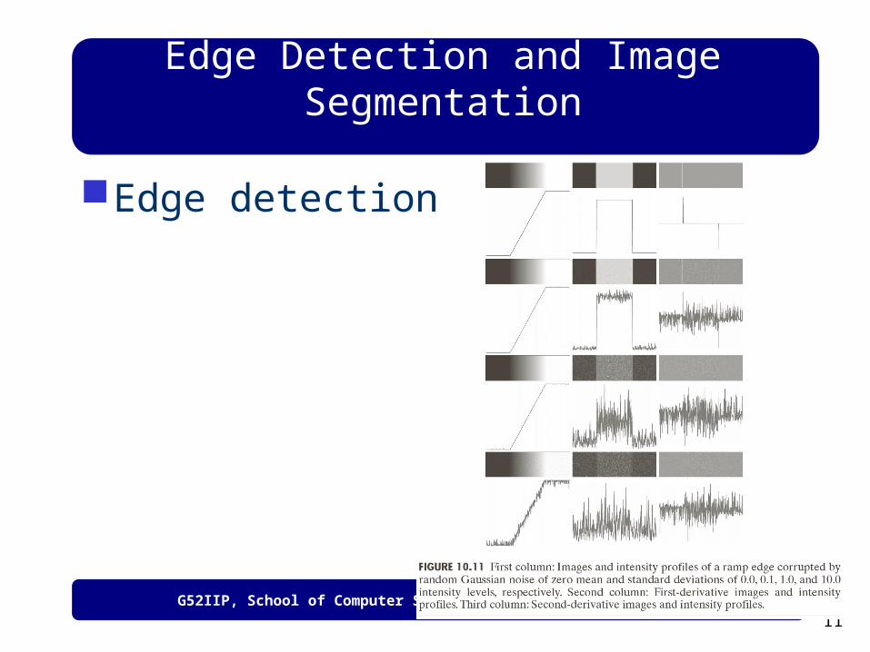
Edge detection

G52IIP, School of Computer Science, University of Nottingham
12
Edge Detection and Image Segmentation
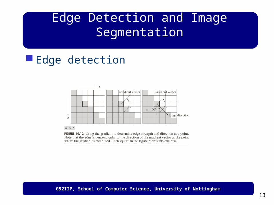
Edge detection
Gradient operators
Magnitude of the gradient
Direction of the gradient vector
y
f
x
f
G
Gf
y
x
21
22yx GGf yx GGf
x
y
G
Gyx 1tan,
G52IIP, School of Computer Science, University of Nottingham
13
Edge Detection and Image Segmentation
Edge detection

G52IIP, School of Computer Science, University of Nottingham
14
Edge Detection and Image Segmentation
Edge detection
Gy
Gx

G52IIP, School of Computer Science, University of Nottingham
15
Edge Detection and Image Segmentation
Edge detection
GyGx

G52IIP, School of Computer Science, University of Nottingham
16
Edge Detection and Image Segmentation
Edge detection

G52IIP, School of Computer Science, University of Nottingham
17
Edge Detection and Image Segmentation
Edge detection

G52IIP, School of Computer Science, University of Nottingham
18
Edge Detection and Image Segmentation
Edge detection

G52IIP, School of Computer Science, University of Nottingham
19
Edge Detection and Image Segmentation
Edge detection

G52IIP, School of Computer Science, University of Nottingham
20
Edge Detection and Image Segmentation
Edge detection
Laplacian
Laplacian of a 2d function f(x,y) is a 2nd order derivative defined as
Masks used to compute Laplacian
2
2
2
22
y
f
x
ff

G52IIP, School of Computer Science, University of Nottingham
21
Edge Detection and Image Segmentation
Edge detection
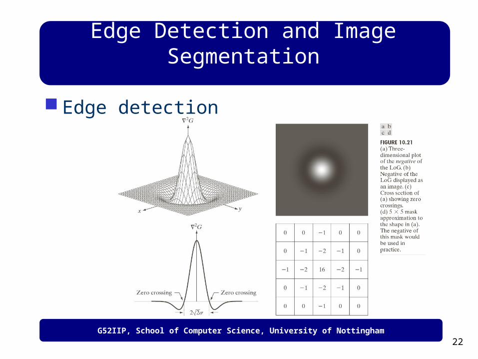
Laplacian of gaussian (LoG)
Because these kernels are approximating a second derivative measurement on the image, they are very sensitive to noise. To counter this, the image is often Gaussian smoothed before applying the Laplacian filter. This pre-processing step reduces the high frequency noise components prior to the differentiation step.
In fact, since the convolution operation is associative, we can convolve the Gaussian smoothing filter with the Laplacian filter first, and then convolve this hybrid filter with the image to achieve the required result. Doing things this way has two advantages:
Since both the Gaussian and the Laplacian kernels are usually much smaller than the image, this method usually requires far fewer arithmetic operations.
The LoG (`Laplacian of Gaussian') kernel can be precalculated in advance so only one convolution needs to be performed at run-time on the image.
G52IIP, School of Computer Science, University of Nottingham
22
Edge Detection and Image Segmentation
Edge detection

G52IIP, School of Computer Science, University of Nottingham
23
Edge Detection and Image Segmentation
Edge detection
Zero Crossing Detector (http://homepages.inf.ed.ac.uk/rbf/HIPR2/zeros.htm)
The zero crossing detector looks for places in the Laplacian of an image where the value of the Laplacian passes through zero - i.e. points where the Laplacian changes sign. Such points often occur at `edges' in images - i.e. points where the intensity of the image changes rapidly, but they also occur at places that are not as easy to associate with edges.
It is best to think of the zero crossing detector as some sort of feature detector rather than as a specific edge detector.

G52IIP, School of Computer Science, University of Nottingham
24
Edge Detection and Image Segmentation
Edge detection
Zero Crossing Detector
The core of the zero crossing detector is the Laplacian of Gaussian filter, `edges' in images give rise to zero crossings in the LoG output.

G52IIP, School of Computer Science, University of Nottingham
25
Edge Detection and Image Segmentation
Edge detection Zero Crossing Detector
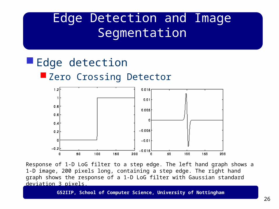
Response of 1-D LoG filter to a step edge. The left hand graph shows a 1-D image, 200 pixels long, containing a step edge. The right hand graph shows the response of a 1-D LoG filter with Gaussian standard deviation 3 pixels.
G52IIP, School of Computer Science, University of Nottingham
26
Edge Detection and Image Segmentation
Edge detection Zero Crossing Detector
Response of 1-D LoG filter to a step edge. The left hand graph shows a 1-D image, 200 pixels long, containing a step edge. The right hand graph shows the response of a 1-D LoG filter with Gaussian standard deviation 3 pixels.

G52IIP, School of Computer Science, University of Nottingham
27
Edge Detection and Image Segmentation
Edge detection Zero Crossing Detector
G52IIP, School of Computer Science, University of Nottingham
28
Edge Detection and Image Segmentation
Edge detection
Canny Edge Detector (http://homepages.inf.ed.ac.uk/rbf/HIPR2/canny.htm) The Canny operator works in a multi-stage process. First of all the image is smoothed by Gaussian convolution. Then a simple 2-D first derivative operator (somewhat like the Roberts
Cross) is applied to the smoothed image to highlight regions of the image with high first spatial derivatives. Edges give rise to ridges in the gradient magnitude image.
The algorithm then tracks along the top of these ridges and sets to zero all pixels that are not actually on the ridge top so as to give a thin line in the output, a process known as non-maximal suppression.
The tracking process exhibits hysteresis controlled by two thresholds: T1 and T2, with T1 > T2.
Tracking can only begin at a point on a ridge higher than T1. Tracking then continues in both directions out from that point until the height of the ridge falls below T2.
This hysteresis helps to ensure that noisy edges are not broken up into multiple edge fragments.
G52IIP, School of Computer Science, University of Nottingham
29
Edge Detection and Image Segmentation
Region Segmentation
Region-based segmentation methods attempt to partition or group regions according to common image properties. These image properties consist of
1. Intensity values from original images, or computed values based on an image operator
2. Textures or patterns that are unique to each type of region3. Spectral profiles that provide multidimensional image data
Elaborate systems may use a combination of these properties to segment images, while simpler systems may be restricted to a minimal set on properties depending of the type of data available.

G52IIP, School of Computer Science, University of Nottingham
30
Edge Detection and Image Segmentation
Region Segmentation Thresholding

G52IIP, School of Computer Science, University of Nottingham
31
Edge Detection and Image Segmentation
Region Segmentation Thresholding
G52IIP, School of Computer Science, University of Nottingham
32
Edge Detection and Image Segmentation
Region Splitting and Merging
The basic idea of region splitting is to break the image into a set of disjoint regions which are coherent within themselves:
Initially take the image as a whole to be the area of interest. Look at the area of interest and decide if all pixels contained in the region satisfy
some similarity constraint. If TRUE then the area of interest corresponds to a region in the image. If FALSE split the area of interest (usually into four equal sub-areas) and consider
each of the sub areas as the area of interest in turn.
This process continues until no further splitting occurs. In the worst case this happens when the areas are just one pixel in size.
This is a divide and conquer or top down method.
If only a splitting schedule is used then the final segmentation would probably contain many neighbouring regions that have identical or similar properties.
Thus, a merging process is used after each split which compares adjacent regions and merges them if necessary. Algorithms of this nature are called split and merge algorithms.

G52IIP, School of Computer Science, University of Nottingham
33
Edge Detection and Image Segmentation
Region Splitting and Merging

G52IIP, School of Computer Science, University of Nottingham
34
Edge Detection and Image Segmentation
Region Splitting and Merging
G52IIP, School of Computer Science, University of Nottingham
35
Edge Detection and Image Segmentation
Region Growing
Region growing approach is the opposite of the split and merge approach:
An initial set of small areas are iteratively merged according to similarity constraints.
Start by choosing an arbitrary seed pixel and compare it with neighbouring pixels.
Region is grown from the seed pixel by adding in neighbouring pixels that are similar, increasing the size of the region.
When the growth of one region stops we simply choose another seed pixel which does not yet belong to any region and start again.
This whole process is continued until all pixels belong to some region.
A bottom up method.

G52IIP, School of Computer Science, University of Nottingham
36
Edge Detection and Image Segmentation
Region Growing

G52IIP, School of Computer Science, University of Nottingham
37
Edge Detection and Image Segmentation
Region Growing
However starting with a particular seed pixel and letting this region grow completely before trying other seeds biases the segmentation in favour of the regions which are segmented first.
This can have several undesirable effects:
Current region dominates the growth process -- ambiguities around edges of adjacent regions may not be resolved correctly.
Different choices of seeds may give different segmentation results.
Problems can occur if the (arbitrarily chosen) seed point lies on an edge.

G52IIP, School of Computer Science, University of Nottingham
38
Edge Detection and Image Segmentation
Region Growing
To counter the above problems, simultaneous region growing techniques have been developed.
Similarities of neighbouring regions are taken into account in the growing process.
No single region is allowed to completely dominate the proceedings.
A number of regions are allowed to grow at the same time. similar regions will gradually coalesce into expanding regions. Control of these methods may be quite complicated but efficient
methods have been developed. Easy and efficient to implement on parallel computers.

G52IIP, School of Computer Science, University of Nottingham
39
Edge Detection and Image Segmentation
Region Growing
To counter the above problems, simultaneous region growing techniques have been developed.
Similarities of neighbouring regions are taken into account in the growing process.
No single region is allowed to completely dominate the proceedings.
A number of regions are allowed to grow at the same time. similar regions will gradually coalesce into expanding regions. Control of these methods may be quite complicated but efficient
methods have been developed. Easy and efficient to implement on parallel computers.

G52IIP, School of Computer Science, University of Nottingham
40
Edge Detection and Image Segmentation
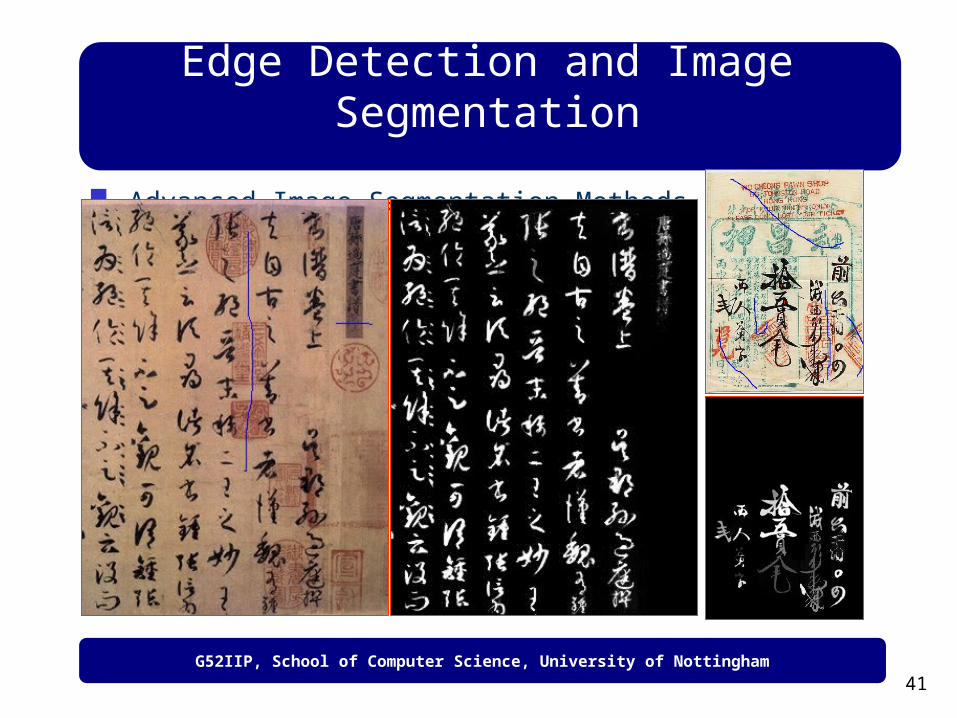
Advanced Image Segmentation Methods
Segment the foreground objects
G52IIP, School of Computer Science, University of Nottingham
41
Edge Detection and Image Segmentation
Advanced Image Segmentation Methods

G52IIP, School of Computer Science, University of Nottingham
42
Edge Detection and Image Segmentation
Advanced Image Segmentation Image editing (synthesis/composition)

G52IIP, School of Computer Science, University of Nottingham
43
Edge Detection and Image Segmentation
Connected Components Labeling (http://homepages.inf.ed.ac.uk/rbf/HIPR2/label.htm)

G52IIP, School of Computer Science, University of Nottingham
44
Identify Individual Object
Connected Component Labeling: Give pixels belonging to the same object the same label (grey level or color)

G52IIP, School of Computer Science, University of Nottingham
45
Identify Individual Object
Connected component labelling works by scanning an image, pixel-by-pixel (from top to bottom and left to right) in order to identify connected pixel regions, i.e. regions of adjacent pixels which share the same set of intensity values.
G52IIP, School of Computer Science, University of Nottingham
46
Identify Individual Object
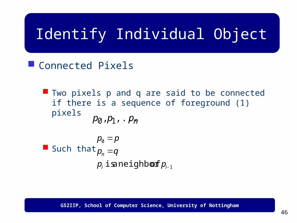
Connected Pixels
Two pixels p and q are said to be connected if there is a sequence of foreground (1) pixels
Such that
nppp ,...., 10
1
0
ofneighbor a is
ii
n
pp
qp
pp

G52IIP, School of Computer Science, University of Nottingham
47
Identify Individual Object
Pixel Neighbors
0 1 0
1 p 1
0 1 0
Four nearest neighbors
1 1 1
1 p 1
1 1 1
Eight nearest neighbors

G52IIP, School of Computer Science, University of Nottingham
48
Identify Individual Object
4- and 8-Connected Pixels
When only the four nearest neighbors are considered part of the neighborhood, then pixels p and q are said to be “4-connected”
When the 8 nearest neighbors are considered part of the neighborhood, then pixels p and q are said to be “8-connected”
4-connected 8-connected

G52IIP, School of Computer Science, University of Nottingham
49
Labelling Algorithm
The connected components labeling operator scans the image by moving along a row until it comes to a point p (where p denotes the pixel to be labeled at any stage in the scanning process) for which V={1}. When this is true, it examines the four neighbors of p which have already been encountered in the scan (in the case of 8-connectivity, the neighbors (i) to the left of p, (ii) above it, and (iii and iv) the two upper diagonal terms). Based on this information, the labeling of p occurs as follows:
If all four neighbors are 0, assign a new label to p, else
if only one neighbor has V={1}, assign its label to p, else
if more than one of the neighbors have V={1}, assign one of the labels to p and make a note of the equivalences.
After completing the scan, the equivalent label pairs are sorted into equivalence classes and a unique label is assigned to each class.
As a final step, a second scan is made through the image, during which each label is replaced by the label assigned to its equivalence classes. For display, the labels might be different graylevels or colors.

G52IIP, School of Computer Science, University of Nottingham
50
Labelling Algorithm
Example (8-connectivity)
1 1 1 1
1 1
1 1
1 1
1
1 1 1
1 1 2 2
1 1
1 1
3 1
3
3 3 3
Equivalent labels
{1, 2}
Original Binary Image After first scan

G52IIP, School of Computer Science, University of Nottingham
51
Labelling Algorithm
Example (8-connectivity)
1 1 2 2
1 1
1 1
3 1
3
3 3 3
Equivalent labels
{1, 2}
After 1st scan
1 1 1 1
1 1
1 1
2 1
2
2 2 2
Final label
1: {1, 2}2: {3}
After 2nd scan (two individual objects/regions have been identified)

G52IIP, School of Computer Science, University of Nottingham
52
Describe Objects
Some useful features can be extracted once we have connected components, including
Area Centroid Extremal points, bounding box Circularity Spatial moments

G52IIP, School of Computer Science, University of Nottingham
53
Describe Objects
Area
Centroid
Ryx
A),(
1
Ryx
A xx),(
1
Ryx
A yy),(
1