generation and characterization of sub … and characterization of sub-70 isolated attosecond pulses...
TRANSCRIPT

GENERATION AND CHARACTERIZATION OF SUB-70 ISOLATED ATTOSECOND PULSES
by
QI ZHANG B.S. University of Science of Technology of China, 2007
M.S. Kansas State University, 2009
A dissertation submitted in partial fulfillment of the requirements for the degree of Doctor of Philosophy in the College of Optics & Photonics at the University of Central Florida
Orlando, Florida
Summer Term 2014
Major Professor: Zenghu Chang

©2014 Qi Zhang
ii

ABSTRACT
Dynamics occurring on microscopic scales, such as electronic motion inside atoms and
molecules, are governed by quantum mechanics. However, the Schrödinger equation is usually
too complicated to solve analytically for systems other than the hydrogen atom. Even for some
simple atoms such as helium, it still takes months to do a full numerical analysis. Therefore,
practical problems are often solved only after simplification. The results are then compared with
the experimental outcome in both the spectral and temporal domain. For accurate experimental
comparison, temporal resolution on the attosecond scale is required. This had not been achieved
until the first demonstration of the single attosecond pulse in 2001. After this breakthrough,
“attophysics” immediately became a hot field in the physics and optics community.
While the attosecond pulse has served as an irreplaceable tool in many fundamental
research studies of ultrafast dynamics, the pulse generation process itself is an interesting topic in
the ultrafast field. When an intense femtosecond laser is tightly focused on a gaseous target,
electrons inside the neutral atoms are ripped away through tunneling ionization. Under certain
circumstances, the electrons are able to reunite with the parent ions and release photon bursts
lasting only tens to hundreds of attoseconds. This process repeats itself every half cycle of the
driving pulse, generating a train of single attosecond pulses which lasts longer than one
femtosecond. To achieve true temporal resolution on the attosecond time scale, single isolated
attosecond pulses are required, meaning only one attosecond pulse can be produced per driving
pulse.
Up to now, there are only a few methods which have been demonstrated experimentally
to generate isolated attosecond pulses. Pioneering work generated single attosecond pulse using a
iii

carrier-envelope phase-stabilized 3.3 fs laser pulse, which is out of reach for most research
groups. An alternative method termed as polarization gating generated single attosecond pulses
with 5 fs driving pulses, which is still difficult to achieve experimentally. Most recently, a new
technique termed as Double Optical Gating (DOG) was developed in our group to allow the
generation of single attosecond pulse with longer driving pulse durations. For example, isolated
150 as pulses were demonstrated with a 25 fs driving laser directly from a commercially-
available Ti:Sapphire amplifier. Isolated attosecond pulses as short as 107 as have been
demonstrated with the DOG scheme before this work. Here, we employ this method to shorten
the pulse duration even further, demonstrating world-record isolated 67 as pulses.
Optical pulses with attosecond duration are the shortest controllable process up to now
and are much faster than the electron response times in any electronic devices. In consequence, it
is also a challenge to characterize attosecond pulses experimentally, especially when they feature
a broadband spectrum. Similar challenges have previously been met in characterizing
femtosecond laser pulses, with many schemes already proposed and well-demonstrated
experimentally. Similar schemes can be applied in characterizing attosecond pulses with narrow
bandwidth. The limitation of these techniques is presented here, and a method recently
developed to overcome those limitations is discussed.
At last, several experimental advances toward the characterization of the isolated 25 as
pulses, which is one atomic unit time, are discussed briefly.
iv

ACKNOWLEDGMENTS
I am blessed to be able to join in this exciting group and it has been a tough and yet
fruitful five years for me.
It is very helpful and productive to work with my colleagues. Particularly, Dr. Zenghu
Chang is my major advisor and has given me countless useful guidance through my PhD study. I
also want to thank Dr. Kun Zhao who introduced me to the research from the beginning and
worked with me for many late nights for our best datasets. All my skills and methods to solve
problems are almost directly learned from him or heavily affected by the experience of working
with him. I also want to thank Dr. Yi Wu who built and maintained the laser—my experiments
wouldn’t go anywhere without his help; Dr. Michael Chini who gave me a lot of help in
understanding physical principles hidden under the experimental data; Yang Wang who worked
with me closely in this research project. I also like to thank Dr. Xiaowei Wang, Yan Chen, Jie Li,
Huaping Zang, Eric Cunningham for all their kinds of support and helpful discussions. I also
worked with Prof. Chaoming Li, Prof. Jianhua Zeng, Xianglin Wang and Peng Xu within the last
year of my PhD. I would like to thank them for their work.
I have also been very fortunate to work with several former colleagues during the first
couple of years during my PhD period. They are Dr. He Wang, Dr. Steve Gilbertson, Dr. Sabih
Khan, Dr. Shouyuan Chen, Dr. Chenxia Yun, and Dr. Baozhen Zhao. They all helped me in one
way or another. Their kindness is much appreciated. I also acknowledge the effort and support
from the technical support staff at both Kansas State University and University of Central
Florida.
v

I would also like to thank Prof. Peter J. Delfyett, Prof. Romain M. Gaume, and Prof.
Haripada Saha for agreeing to serve on my dissertation committee.
I also want to thank my wife Dr. Suhao Han for her understanding and support. We have
been long distance for a very long time and I have spent way more time in the laboratory than
with her during the last five years. But she has been very patient with me and my work couldn’t
be done today without her.
Finally, I want to thank my parents in China for their life-long support. I haven’t been
back to China in almost five years and am deeply owed to them. I would like to acknowledge
their spiritual support during my whole life.
vi

TABLE OF CONTENTS
LIST OF FIGURES ....................................................................................................................... ix
LIST OF TABLES ....................................................................................................................... xix
CHAPTER 1 INTRODUCTION ................................................................................................. 1
CHAPTER 2 HIGH-ORDER HARMONIC GENERATION .................................................... 4
2.1 The Three Step Model ...................................................................................................... 5
2.2 Attosecond Pulse Train .................................................................................................. 11
CHAPTER 3 ISOLATED ATTOSECOND PULSES .............................................................. 14
3.1 Few-Cycle Femtosecond Laser ...................................................................................... 15
3.2 Polarization Gating ......................................................................................................... 18
3.3 Double Optical Gating ................................................................................................... 25
CHAPTER 4 TEMPORAL CHARACTERIZATION OF ATTOSECOND PULSES ............. 28
4.1 The Principle of Attosecond Streaking .......................................................................... 28
4.2 Complete Reconstruction of Attosecond Bursts ............................................................ 33
4.3 Phase Retrieval by Omega Oscillation Filtering ............................................................ 34
4.4 Reconstruction Error ...................................................................................................... 37
CHAPTER 5 EXPERIMENTAL CONFIGURATION ............................................................ 39
5.1 Experimental Configuration ........................................................................................... 39
5.2 Principle of Magnetic Bottle Energy Spectrometer ....................................................... 43
vii

5.3 Resolution of MBES ...................................................................................................... 48
CHAPTER 6 GENERATION AND CHARACTERIZATION OF 67 ATTOSECOND PULSE
57
6.1 Generation and Characterization of 67 Isolated Attosecond Pulse ................................ 57
CHAPTER 7 ROUTE TO ATTOSEOCND PULSES WITH ONE ATOMIC UNIT OF TIME
64
7.1 Broadband Supercontinuum Generation with Lens Focusing........................................ 65
7.2 Characterizing the Contrast of 25 Attosecond Isolated Pulses ...................................... 68
7.3 Suppressing the Driving Laser with Microchannel Plate ............................................... 80
CHAPTER 8 CONCLUSIONS AND OUTLOOK ................................................................... 90
APPENDIX A: LIST OF PUBLICATIONS ................................................................................ 91
APPENDIX B: COPYRIGHT PERMISSION ............................................................................. 95
LIST OF REFERENCES ............................................................................................................ 107
viii

LIST OF FIGURES
Figure 1.1 Time scale for different dynamics. (a) Picosecond time scale for rotational motion of
the atoms inside molecules. (b) Femtosecond time scale for vibrational motion of
the atoms inside molecules. (c) Electron dynamics inside atoms. .......................... 2
Figure 2.1(a) A schematic drawing illustrating the three step model (i) Tunnel ionization. (ii)
Acceleration by the driving field. (iii) Recombination with the parent ion. (b) A
schematic plot of a typical intensity spectrum from high-order harmonic
generation. ............................................................................................................... 5
Figure 2.2 Numerically calculated recombination time as a function of the emission time for a
tunnel-ionized electron. (b) The kinetic energy of the returned electron before it
recombines with the parent ion, as a function of the emission time. ...................... 8
Figure 2.3 The kinetic energy of the recombined electron as a function of recombination time.
The short and long trajectories are labeled with blue and red colors separately. . 10
Figure 2.4 The intrinsic chirp as a function of the photon energy for short trajectory only,
assuming 0.75 𝜇𝜇𝜇𝜇 central wavelength and assuming 1 × 10¹⁵ 𝑊𝑊/𝑐𝑐𝜇𝜇2 peak
intensity. ................................................................................................................ 10
Figure 2.5 Schematic drawing of a typical experimental configuration for generating high-order
harmonics and detecting photoelectron spectra. ................................................... 12
Figure 2.6 Experimental photoelectron spectrum with linearly polarized driving laser
(Ti:Sapphire laser with 1 millijoule pulse energy and 25 femtosecond pulse
duration). The cutoff at about 50 eV are from Aluminum filter which was used to
block the remaining driving field. ......................................................................... 13
ix
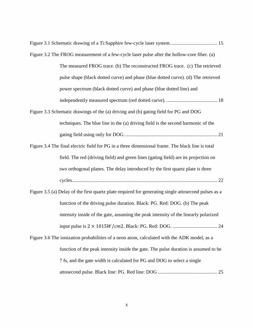
Figure 3.1 Schematic drawing of a Ti:Sapphire few-cycle laser system. ..................................... 15
Figure 3.2 The FROG measurement of a few-cycle laser pulse after the hollow-core fiber. (a)
The measured FROG trace. (b) The reconstructed FROG trace. (c) The retrieved
pulse shape (black dotted curve) and phase (blue dotted curve). (d) The retrieved
power spectrum (black dotted curve) and phase (blue dotted line) and
independently measured spectrum (red dotted curve). ......................................... 18
Figure 3.3 Schematic drawings of the (a) driving and (b) gating field for PG and DOG
techniques. The blue line in the (a) driving field is the second harmonic of the
gating field using only for DOG. .......................................................................... 21
Figure 3.4 The final electric field for PG in a three dimensional frame. The black line is total
field. The red (driving field) and green lines (gating field) are its projection on
two orthogonal planes. The delay introduced by the first quartz plate is three
cycles..................................................................................................................... 22
Figure 3.5 (a) Delay of the first quartz plate required for generating single attosecond pulses as a
function of the driving pulse duration. Black: PG. Red: DOG. (b) The peak
intensity inside of the gate, assuming the peak intensity of the linearly polarized
input pulse is 2 × 10¹⁵𝑊𝑊/𝑐𝑐𝜇𝜇2. Black: PG. Red: DOG. .................................... 24
Figure 3.6 The ionization probabilities of a neon atom, calculated with the ADK model, as a
function of the peak intensity inside the gate. The pulse duration is assumed to be
7 fs, and the gate width is calculated for PG and DOG to select a single
attosecond pulse. Black line: PG. Red line: DOG ................................................ 25
x

Figure 3.7 The photoelectron spectra of HHG generated with linear polarized driving laser (black
line) and DOG driving laser (red line). The 300 nm thick Aluminum filter is used
to block the remaining driving pulse and transmitting the XUV. ......................... 27
Figure 4.1 A schematic drawing of the RABITT photon transition. The sideband (dashed line)
can be produced by one XUV photon adding one IR photon. .............................. 30
Figure 4.2 A schematic drawing depicting the principle of attosecond streaking (a) XUV (blue)
and streaking field (red dashed) (b) The streaking trace obtained by scanning the
delay between XUV and streaking field and recording photoelectron spectra at
each delay.............................................................................................................. 32
Figure 5.1 A schematic drawing of the experimental configuration for the attosecond streaking
experiment based on a Magnetic Bottle Energy Spectrometer (MBES). BS: Beam
Splitter; QP: Quartz Plate; M: Silver Mirror; CM1: convex mirror with -150 mm
focal length, CM2: concave mirror with 250 mm focal length; GC: Gas Cell; MF:
Metallic Filter; TM: Toroidal Mirror; FM: Flat Mirror; L: Focus Lens; HM: Hole
drilled Mirror; MBES: Magnetic Bottle Electron Energy Spectrometer. ............. 40
Figure 5.2 (a) Diagram of Magnetic Bottle Electron Spectrometer (MBES) with a three-meter-
long flight tube. The XUV beam is focused 1 mm away from the magnet which
produces a highly diverging magnetic field, and a 50 micrometer diameter
stainless steel gas jet is placed on top of the XUV beam. Photoelectrons enter an
aperture with a diameter D and fly through the three-meter-long tube before
reaching the MCP detector. A solenoid coil with 0.8 A current is wrapped around
the flight tube to supply a 10 Gauss magnetic field. A µ-metal tube is placed
outside the flight tube to shield the earth’s magnetic field. (b) An enlarged
xi

schematic diagram of the magnet and aperture. The plot in polar coordinates
shows the photoelectron angular distribution with an asymmetric parameter of
1.4, as defined in equation 5.2. The collection angle of the MBES is calculated to
be 107°. The solid angle within which the photoelectrons can be collected by the
MBES is shown in gray color. (Reprinted from Journal of Electron Spectroscopy
and Related Phenomena, Vol. 195, Q Zhang etc. “High resolution electron
spectrometers for characterizing the contrast of isolated 25 as pulses”, Copyright
(2014), with permission from Elsevier) ................................................................ 45
Figure 5.3 Calculated magnetic field along the z-axis (𝐵𝐵𝐵𝐵). The blue line represents 𝐵𝐵𝐵𝐵 generated
from the permanent magnet, the red line shows 𝐵𝐵𝐵𝐵 from the solenoid, and the
black line is the total field of the two. Inset: comparison of calculation and
measurement of 𝐵𝐵𝐵𝐵 between z from 1 mm to 25 mm. The black solid line is the
calculation and the red line with dot is the measurement. .................................... 46
Figure 5.4 The comparison between the calculation and measurements of 𝐵𝐵𝐵𝐵 in the transverse
plane at distances from 1 to 4 mm. The black line shows the calculated result. The
red and blue dotted lines show 𝐵𝐵𝐵𝐵 from two orthogonal directions in the
transverse plane which is perpendicular to the z axis. .......................................... 47
Figure 5.5 The comparison between the calculation and measurements of 𝐵𝐵𝐵𝐵 in the transverse
plane at distances from 5 to 20 mm. The black line shows the calculated result.
The red and blue dotted lines show 𝐵𝐵𝐵𝐵 from two orthoganal directions separately
in the transverse surface which is perpendicular to the z axis. ............................. 47
xii

Figure 5.6 The calculated ratio between measured energy 𝐸𝐸𝐸𝐸𝐸𝐸𝐸𝐸 and initial electron energy as a
function of emission angle of the photoelectron.(b) The calculated response
function of 100 eV electrons with all possible emission angles. .......................... 50
Figure 5.7 Experimental setup to measure the temporal resolution of the MCP electron detection
system. Laser pulses of 25 fs at 800 nm are focused in air by a lens (f =100 mm)
and generate UV photons at 267 nm. Part of the laser beam is reflected by a beam
splitter (BS) to a photodiode. The laser intensity can be adjusted by a variable
neutral density (ND) filter. A prism separates the 800 and 267 nm beams and the
UV beam is reflected to the MCP detector by a mirror. The detector is housed in a
vacuum chamber. Signals from the photodiode and the MCP were processed by
two CFDs and sent to the TDC as the start and stop signals, respectively. A VME
crate transmits the TDC data to a computer for analysis. (Reproduced with
permission from [DETERMINING TIME RESOLUTION OF
MICROCHANNEL PLATE DETECTORS FOR ELECTRON TIME-OF-
FLIGHT SPECTROMETER, Review of Scientific Instruments 81, 073112
(2009)]. Copyright [2009], AIP Publishing LLC,
http://dx.doi.org/10.1063/1.3463690) ................................................................... 52
Figure 5.8 UV photon TOF spectrum (dots) obtained by the setup shown in Fig.1. The FWHM is
204 ps, obtained by fitting the experimental spectrum with a Gaussian function
𝐴𝐴𝐴𝐴 − (𝑡𝑡 − 𝑡𝑡0)2/2𝑤𝑤2, (solid curve) so that ΔT(FWHM) = 2.355w. The MCP
voltage was 1800 V. The threshold of CFD 9327 was -75 mV. Inset: TDC
spectrum (dots) obtained by feeding photodiode output through both 9327 and
583 CFDs. The FWHM is 54 ps, obtained by fitting the experimental spectrum
xiii

with a Gaussian function (solid curve). (Reprinted from Q. Zhang, K. Zhao, and
Z. Chang, "Determining Time Resolution of Microchannel Plate Detectors for
Electron Time-of-Flight Spectrometer" Review of Scientific Instruments 81,
073112 (2009))...................................................................................................... 53
Figure 5.9 The comparison of experiment and simulation for harmonic peak at 32.6 eV. (a) The
convolution (blue) of the MBES response function at 32.6 eV with 30 V retarding
potential (black) and harmonic spectrum (red).(b) The convolution (blue) of the
MBES response function at 32.6 eV with no retarding potential (black) and
harmonic spectrum (red) (c) Comparison of experimental measurement of
harmonic at 32.6 eV with 30 V retarding potential (red) and convolution (blue)
from (a). (d) Comparison of experimental measurement of harmonic at 32.6 eV
with no retarding potential (black) and convolution (red) from (b)...................... 55
Figure 5.10 The comparison of experiment and simulation for harmonic peak at 65.7 eV. (a) The
convolution (blue) of the MBES response function at 65.7 eV with 60 V retarding
potential (black) and harmonic spectrum (red).(b) The convolution (blue) of the
MBES response function at 65.7 eV with no retarding potential (black) and
harmonic spectrum (red) (c) Comparison of experimental measurement of
harmonic at 65.7 eV with 60 V retarding potential (red) and convolution (blue)
from (a). (d) Comparison of experimental measurement of harmonic at 65.7 eV
with no retarding potential (black) and convolution (red) from (b)...................... 56
Figure 6.1 The transmission (black solid line) and material GDD (blue dash-dotted line) of (a)
aluminum (b) zirconium (c) titanium, and (d) molybdenum. ............................... 59
xiv

Figure 6.2 XUV photoelectron spectrum generated by DOG in Ne gas with six different
pressures. The length of the gas cell is 1 mm. The peak intensity at the center of
the polarization gate is about 1 × 10¹⁵𝑊𝑊/𝑐𝑐𝜇𝜇2. (Reproduced from Zhao, Zhang,
Chini, Wu, Wang & Chang, “Tailoring a 67 attosecond pulse through
advantageous phase-mismatch. Optics Letters”, 37(18), 3891, 2012) ................. 61
Figure 6.3 Attosecond intrinsic chirp compensated by a 300 nm Zr filter. The spectrum is
specially chosen to cover the area where the attochirp is best compensated. Black
solid line: XUV spectrum taken with 300 nm Zr filter. Red dashed line: intrinsic
chirp of the attosecond pulses. Blue dash-dotted line: GDD of 300 nm Zr filter. 62
Figure 6.4 Characterization of a 67 as XUV pulse. (a) Streaked photoelectron spectrogram
obtained experimentally. (b) Filtered 𝐼𝐼𝐼𝐼𝐼𝐼𝐼𝐼, 𝜏𝜏 trace (left) from the spectrogram in
(a) and the retrieved 𝐼𝐼𝐼𝐼𝐼𝐼𝐼𝐼, 𝜏𝜏 trace (right). (c) Photoelectron spectrum obtained
experimentally (thick grey solid) and retrieved spectra and spectral phases from
PROOF (blue solid) and FROG-CRAB (red dashed). (d) Retrieved temporal
profiles and phases from PROOF (blue solid) and FROG-CRAB (red dashed).
(Reproduced from Zhao, Zhang, Chini, Wu, Wang & Chang, Tailoring a 67
attosecond pulse through advantageous phase-mismatch. Optics Letters, 37(18),
3891, 2012) ........................................................................................................... 63
Figure 7.1 Performance of the lens focusing a 7 fs TL input pulse, with a 3 mm beam waist on
the lens surface. (a) The electric field in the temporal domain. Red solid line:
input field. Blue dashed line: electric field at the focus. (b) The laser spectra. Red
solid line: input field. Blue dashed line: electric field at the focus. ...................... 66
xv

Figure 7.2 A schematic drawing of the experimental configuration with the lens focusing
configuration. BS: Beam Splitter; QP: Quartz Plate; M: Silver Mirror; L: lens
with 140 mm focal length; GC: Gas Cell; MF: Metallic Filter; TM: Toroidal
Mirror; HM: Hole drilled Mirror; MBES: Magnetic Bottle Electron Energy
Spectrometer. ........................................................................................................ 67
Figure 7.3 The supercontinuum spectrum measured with a 140 mm focal lens and a 300 nm
molybdenum filter. The cutoff has extended to 180 eV photon energy. (b) The
Fourier-transformed temporal spectrum assuming a TL pulse duration for the
spectrum in (a). The FWHM is 40 as. ................................................................... 68
Figure 7.4 Effects of the response function on characterizing satellite pulses (1% satellite pulse is
assumed). (a) The blue solid line shows the input temporal pulse. The red dashed
line with dot is the retrieved temporal pulse from the streaking trace. (b) The blue
solid line shows the spectrum of the input pulse, and the red dashed line is the
convoluted spectrum in a 3 m TOF. Inset shows the enlarged spectra from 120 to
140 eV. .................................................................................................................. 71
Figure 7.5(a) Ratio of the energy calculated from the flight time (ETOF) to the real value (Ei) as a
function of the emission angle. Electrons with emission angles larger than 107°
cannot be detected by the MCP. (b) Energy distribution of 180 eV monoenergetic
electrons calculated assuming the angular distribution of Ne photoionization with
an asymmetric parameter of 1.4, which is referred to as the response function. The
solid line is for a spectrometer with 3 m flight distance; and the dashed line is for
an 8 m TOF. (Reprinted from Q Zhang, K. Zhao, and Z. Chang, “High resolution
electron spectrometers for characterizing the contrast of isolated 25 as pulses”.
xvi

Journal of Electron Spectroscopy and Related Phenomena, 195, pp 48-54. DOI:
10.1016/j.elspec.2014.05.008 ) ............................................................................. 73
Figure 7.6 (a) Collection angle and (b) collection efficiency as functions of the electron energy
for different pinhole diameters.............................................................................. 75
Figure 7.7 Response function calculated with a 0.25 mm pinhole in the 8 m TOF, for 180 eV
electrons (blue solid line). The response function without is plotted with red
dashed line for comparison. .................................................................................. 76
Figure 7.8 Comparison of the retrieved satellite pulse contrast limited by MBES resolution with
real values. The red line with circles shows the retrieved contrast with an 8 m
TOF. The blue line with diamonds shows the real value of 1% contrast as a
comparison. ........................................................................................................... 77
Figure 7.9 Experimental evaluation of the collection efficiency of the 0.15 mm and 0.5 mm cone.
(a) The spectra taken with 0.15 mm (black solid) and 0.5 mm (red solid) cone size
under the same condition. The 200 nm thick Be filter was used to block the IR
and select the energy range between 0~90eV. (b) The collection efficiency
dependence on the electron energy for 0.15 mm. The black line shows the
experimental result calculated from (a) and the red line shows the calculation
from Fig 7.6. ......................................................................................................... 78
Figure 7.10 Schematic drawings of several common techniques for separating the driving IR and
the generated XUV from the HHG. (a) Metallic filter. (b) Annular driving beam
(c) multilayer beam splitter or Si/SiC plate on the Brewster Angle (d) Grating
pairs. ...................................................................................................................... 82
xvii

Figure 7.11 Schematic drawing of the principle of the MCP filter. The diameter of each MCP
channel is comparable to the wavelength of the IR but much larger than that of the
XUV. The red (blue) lines indicate the IR (XUV) beam. The 0th, ±1st order
diffractions are labeled by black arrows. (Reprinted from Q Zhang, K. Zhao, J. Li,
M. Chini, Y. Cheng, Y. Wu, E. Cunningham, and Z. Chang, “Suppression of
Driving Laser in High Harmonic Generation with a Microchannel Plate”. Opt.
Lett. Vol. 39, Issue 12, pp. 3670-3673 (2014),
http://dx.doi.org/10.1364/OL.39.003670) ............................................................. 84
Figure 7.12 The zero-order transmission of the MCP for (a) XUV photons and (b) visible or
longer wavelengths. The red line in (a) is the transmission measured with a 300
nm Zr filter and a 300 nm Al filter. ...................................................................... 85
Figure 7.13(a) RABBITT spectrograms with (left) and without (right) MCP filter. (b) The
relative delay for sideband maxima as the function of the photoelectron energy.
The red squares were taken with Al and MCP filter, and the blue dots were taken
with Al filter only. The linear fits for each dataset were plotted in the solid and
dashed lines with the same color. (Reprinted from Q Zhang, K. Zhao, J. Li, M.
Chini, Y. Cheng, Y. Wu, E. Cunningham, and Z. Chang, “Suppression of Driving
Laser in High Harmonic Generation with a Microchannel Plate”. Opt. Lett. Vol.
39, Issue 12, pp. 3670-3673 (2014), http://dx.doi.org/10.1364/OL.39.003670) .. 89
xviii

LIST OF TABLES
Table 7.1 The comparison between different methods for separating the driving laser and the
generated XUV from the HHG. (Metallic filter, Annular driving beam, multilayer
beam splitter) ........................................................................................................ 87
Table 7.2 The comparison between different methods for separating the driving laser and the
generated XUV from the HHG. (Si/SiC plate, Grating pairs, MCP filter) ........... 88
xix

CHAPTER 1 INTRODUCTION
The laser is a device that delivers optical sources in both a spatially- and temporally-
coherent manner. Since its first invention in 1960, the advance of laser technology has
significantly changed and is still changing peoples’ lives [1]–[4]. Due to the coherence of the
laser light, it can be compressed in a very small spatial area and an extremely short period,
making it an ideal tool for studying microscopic phenomena. Today, the focus of a laser light can
reach to a scale of less than one micrometer [5], and the period of a laser pulse can be shorter
than one hundred attoseconds (10-18 s) [6], [7].
Since a laser source can carry a considerable amount of energy in a very short period and
small space, it can be used to alter the status of a microscopic target very quickly. This allows us
to observe the dynamics of the target in the temporal domain, as long as the pulse duration of the
laser is short enough compared to the target response. Fig 1.1 shows different time scales for
different dynamics. For example, laser sources with picosecond duration can be used to study the
rotational movement of the atoms inside molecules, as shown in Fig. 1.1 (a). Starting from the
1990s, along with the appearance of several techniques such as mode-locking, sub-100-
femtosecond (1 fs = 10-15 s) laser sources have become available. They can be used to study fast
vibrational modes inside different type of molecules as shown in Fig. 1.1 (b) [8]–[12]. However,
femtosecond lasers are usually centered at wavelengths of hundreds of nanometer (nm) (e.g., the
widely-used Ti:Sapphire laser has a central wavelength of ~800 nm). Therefore, the shortest laser
pulse duration from a Ti:Sapphire is fundamentally limited by one optical cycle, which is 2-3 fs
[7], [13], [14]. To reach even shorter pulse durations, one unavoidably needs to operate in the
Extreme Ultraviolet (XUV) region.
1

Most recently, an XUV pulse lasting only hundreds of attosecond was demonstrated [15],
symbolizing a breakthrough into the attosecond era. Attosecond pulses can be used to study the
electron dynamics inside atomic, molecular and condensed matter systems [16]–[26]. For
example, it takes an electron in the ground state of a hydrogen atom about 25 as to orbit once
around the proton in the classical picture, as shown in Fig. 1.1 (c).
Figure 1.1 Time scale for different dynamics. (a) Picosecond time scale for rotational motion of the atoms inside molecules. (b) Femtosecond time scale for vibrational motion of the atoms inside molecules. (c) Electron dynamics inside atoms. Unlike commercialized femtosecond or picosecond lasers, an attosecond “laser” source is
not a traditionally-defined laser since there is no amplification process. Actually the attosecond
source comes from a highly nonlinear process caused by the interaction of an intense
electromagnetic field with atoms or molecules, which is termed as High-order Harmonic
Generation (HHG) [27]. In order to observe the HHG, the driving field needs a peak intensity
2

more than 1014 W/cm2. Currently, Ti:Sapphire lasers using Chirped Pulse Amplification (CPA)
are widely used due to their relative high pulse energy and short pulse duration [28], [29] .
However, the HHG process repeats itself every half cycle of the driving laser, leading to
the generation of a train of attosecond pulse. In order to get true attosecond temporal resolution,
a single isolated attosecond pulse is required for, as an example, pump-probe experiments. This
is not a straightforward task. Since the first demonstration of the single attosecond pulse, several
schemes and techniques have been proposed and demonstrated [7], [30]–[33]. Among them, the
Double Optical Gating (DOG) technique proposed recently has been demonstrated
experimentally to generate an isolated 130 attosecond pulse [34]. In this work, the
implementation of DOG is pushed to another level, generating and characterizing a world record
of isolated 67 as pulses [6].
This dissertation will be organized as follows. Chapter 2 introduces the HHG and its
mechanism. Chapter 3 explains in detail the principle of DOG and compares it with its
counterparts. Chapter 4 focuses on two phase retrieval algorithms for temporal characterization
of an attosecond pulse. In Chapter 5, the experimental setup with a high-resolution electron
energy spectrometer for attosecond streaking built at the Institute for the Frontier of Attosecond
Science and Technology (iFAST) is introduced, and simulations on the spectrometer resolution
are compared with experimental results. Chapter 6 presents the experimental results
demonstrating the single 67 as pulse. In Chapter 7, some of the most recent progress towards the
generation of isolated 25 as pulses is discussed. Finally in Chapter 8, a summary of the chapters
is given, and paths for future work are brought up for consideration.
3

CHAPTER 2 HIGH-ORDER HARMONIC GENERATION
High-order harmonic generation was first observed in the late 1980s [27], much earlier
than the first demonstration of single attosecond pulses. A laser with 1067 nm and 50 picosecond
duration was focused on an argon gas target, and a series of odd harmonics of the driving laser
were then observed. The experimental result, obviously differing from the prediction of
perturbation theory, was well explained by the so-called “Three Step Model” brought up in 1993
by Corkum [35]. This model separates the HHG process into three steps: first, the valence
electrons from neutral atoms are tunnel-ionized by the strong electric field of the laser; second,
the free electrons are then accelerated by the laser field; finally, under certain circumstances the
electrons return and recombine with parent ions. The kinetic energy gained during the
accelerating process is then released in the form of photon. A schematic drawing is shown in Fig.
1.1(a).
Due to the non-perturbative nature of this process, the harmonic spectrum from the HHG
usually shows a relative flat area called the “plateau” after the first several orders drop quickly in
intensity [36], [37]. After the plateau, the signal drops quickly again and this area is termed the
“cutoff” of the HHG. The schematic drawing of the HHG can be seen in Fig. 1.1 (b). The cutoff
is the highest energy that the XUV photon can reach, hence limiting the bandwidth of the final
attosecond pulse. A broadband spectrum is not the only requirement to achieve short pulse
durations: additionally, minimal spectral dispersion is also needed. The intrinsic chirp of the
attosecond pulse from the HHG process is also calculated in this chapter.
4

Figure 2.1(a) A schematic drawing illustrating the three step model (i) Tunnel ionization. (ii) Acceleration by the driving field. (iii) Recombination with the parent ion. (b) A schematic plot of a typical intensity spectrum from high-order harmonic generation.
2.1 The Three Step Model
For a simple discussion, a linearly-polarized, plane-wave driving laser is considered here.
Assuming the electric field is polarized in the x-axis direction, its electric field at a given spatial
point can be expressed by
5

𝜀𝜀(𝑡𝑡) = 𝐸𝐸0cos (𝐼𝐼0𝑡𝑡) ( 2.1 )
We further assume that in the first step, the ground state electron tunnels through the
potential barrier instantaneously. After the tunneling, the electron can be treated as a free
electron following classical mechanics. The Coulomb potential of the parent ion can be ignored,
as long as the Keldysh parameter 𝛾𝛾 = �2𝐼𝐼𝑝𝑝𝑚𝑚𝜔𝜔02
𝑒𝑒2𝐸𝐸02 is less than 1 [38]. For our home-built
Ti:Sapphire CPA system centered at 750 nm with 7 fs pulse duration and 1 mJ energy, the
angular frequency 𝐼𝐼0 is 6.4 × 10¹³ 𝑟𝑟𝑟𝑟𝑟𝑟/𝑠𝑠, the ionization potential 𝐼𝐼𝑝𝑝 is 21.5 eV for neon, the
electric field amplitude 𝐸𝐸0 is estimated to be 8.7 × 10¹⁰ 𝑉𝑉/𝜇𝜇 corresponding to a peak intensity
of 1 × 10¹⁵ 𝑊𝑊/𝑐𝑐𝜇𝜇2, and 𝐴𝐴 and 𝜇𝜇 are the electron charge and mass respectively The Keldysh
parameter 𝛾𝛾 is calculated to be 0.45, indicating that our parameters fit well within the tunneling
region.
The free electron motion is treated classically. Therefore, the acceleration of the tunneled
electrons should be
𝑑𝑑2𝑥𝑥𝑑𝑑𝑡𝑡2
= − 𝑒𝑒𝑚𝑚𝜀𝜀(𝑡𝑡) = − 𝑒𝑒
𝑚𝑚𝐸𝐸0cos (𝐼𝐼0𝑡𝑡) ( 2.2 )
.
The equation is then solved for velocity and displacement as a function of time, as seen below:
𝐼𝐼(𝑡𝑡) = 𝑑𝑑𝑥𝑥𝑑𝑑𝑡𝑡
= − 𝑒𝑒𝐸𝐸0𝑚𝑚𝜔𝜔0
[sin(𝐼𝐼0𝑡𝑡) − sin(𝐼𝐼0𝑡𝑡0)] ( 2.3 )
𝑥𝑥(𝑡𝑡) = 𝑒𝑒𝐸𝐸0𝑚𝑚𝜔𝜔0
2 {[cos(𝐼𝐼0𝑡𝑡) − cos(𝐼𝐼0𝑡𝑡0)] + 𝐼𝐼0𝑠𝑠𝑠𝑠𝑠𝑠(𝐼𝐼0𝑡𝑡0)(𝑡𝑡 − 𝑡𝑡0)} ( 2.4 )
Here, 𝑡𝑡0 is the time when the electron is tunnel-ionized. In the third step, the electron recombines
with the parent ion and emits a photon. Solve equation 2.4 using 𝑥𝑥(𝑡𝑡) = 0 for the time 𝑡𝑡, and
6
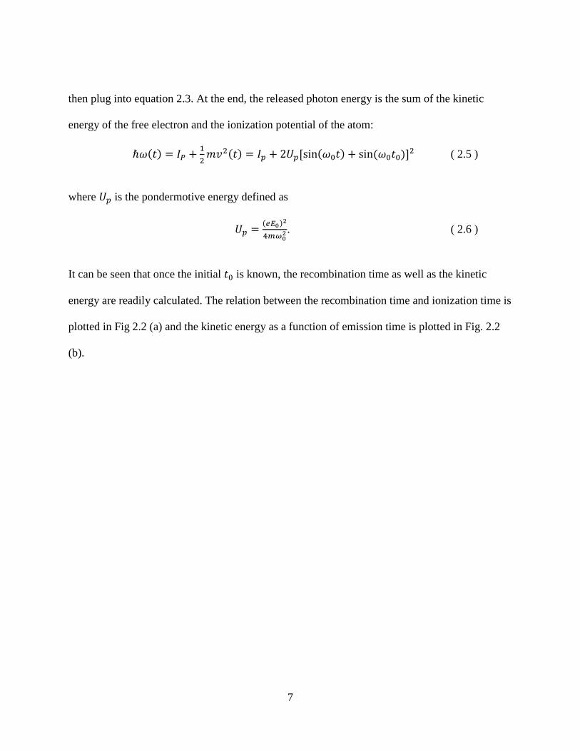
then plug into equation 2.3. At the end, the released photon energy is the sum of the kinetic
energy of the free electron and the ionization potential of the atom:
ℏ𝐼𝐼(𝑡𝑡) = 𝐼𝐼𝑃𝑃 + 12𝜇𝜇𝐼𝐼2(𝑡𝑡) = 𝐼𝐼𝑝𝑝 + 2𝑈𝑈𝑝𝑝[sin(𝐼𝐼0𝑡𝑡) + sin (𝐼𝐼0𝑡𝑡0)]2 ( 2.5 )
where 𝑈𝑈𝑝𝑝 is the pondermotive energy defined as
𝑈𝑈𝑝𝑝 = (𝑒𝑒𝐸𝐸0)2
4𝑚𝑚𝜔𝜔02 . ( 2.6 )
It can be seen that once the initial 𝑡𝑡0 is known, the recombination time as well as the kinetic
energy are readily calculated. The relation between the recombination time and ionization time is
plotted in Fig 2.2 (a) and the kinetic energy as a function of emission time is plotted in Fig. 2.2
(b).
7

Figure 2.2 Numerically calculated recombination time as a function of the emission time for a tunnel-ionized electron. (b) The kinetic energy of the returned electron before it recombines with the parent ion, as a function of the emission time.
From Fig. 2.2 (b), the maximum kinetic energy is 𝐾𝐾𝑚𝑚𝑚𝑚𝑥𝑥 = 3.17𝑈𝑈𝑝𝑝, which is carried by
the electron released at 𝐼𝐼0𝑡𝑡0 = 0.05 × 2𝜋𝜋 rad and returns at 𝐼𝐼0𝑡𝑡 = 0.7 × 2𝜋𝜋 . Thus, the HHG
cutoff is
ℏ𝐼𝐼𝑚𝑚𝑚𝑚𝑥𝑥 = 𝐼𝐼𝑝𝑝 + 3.17𝑈𝑈𝑝𝑝. ( 2.7 )
The ponderomotive energy 𝑈𝑈𝑝𝑝 can be simply expressed as:
𝑈𝑈𝑃𝑃[𝐴𝐴𝑉𝑉] = 9.33 × 10⁻¹⁴𝐼𝐼0𝜆𝜆02 ( 2.8 )
8

in which 𝐼𝐼0 is the peak intensity of the laser in 𝑊𝑊/𝑐𝑐𝜇𝜇2 and 𝜆𝜆0 is the wavelength of the driving
laser in 𝜇𝜇𝜇𝜇. In our cases, if we choose neon as the gas target (𝐼𝐼𝑝𝑝=21.5 eV), the peak intensity of
1 × 10¹⁵ 𝑊𝑊/𝑐𝑐𝜇𝜇2 and central wavelength of 0.75 𝜇𝜇𝜇𝜇 from a Ti:Sapphire laser , the
corresponding cutoff photon energy can be 170 eV. As a reference, the bandwidth required for a
transform-limited Gaussian pulse with a Full Width Half Maximum (FWHM) of 25 as is 150 eV!
Moreover, from Fig. 2.2 (b), there are two “paths” to obtain one final kinetic energy. The
electron released before 0.05 cycle returns later and electron released after that return earlier,
according to the Fig. 2.2 (a). Therefore, the first path is termed as “long trajectory” and the other
as “short trajectory”. The high-order harmonics from the two trajectories exhibit complete
different coherence and diverging angle [39], [40]. The existence of two paths further
complicates the single attosecond pulse. Fortunately, the long trajectories can often be
suppressed by adjusting phase matching conditions.
To calculate the intrinsic chirp, the kinetic energy as function of recombination time is
plotted as below. It can be seen that there is a significant difference between long and short
trajectories: the directions of the slope in Fig. 2.3 are opposite to each other, indicating the
opposite spectral and temporal chirp for the generated XUV pulse from the two paths. The
intrinsic chirp for the short trajectory is calculated from 𝑟𝑟𝑡𝑡 𝑟𝑟𝐾𝐾(𝑡𝑡)� and plotted in Fig. 2.4,
assuming 1 × 10¹⁵ 𝑊𝑊/𝑐𝑐𝜇𝜇2 peak intensity and 0.75 𝜇𝜇𝜇𝜇 central wavelength. It can be seen that
the intrinsic chirp is positive for the short trajectory, which is the case in our experiment;
therefore, negative material chirp should be applied to compensate the intrinsic chirp for
achieving shortest pulse durations. This is very important and will be discussed in more detail in
Chapter 6.
9

Figure 2.3 The kinetic energy of the recombined electron as a function of recombination time. The short and long trajectories are labeled with blue and red colors separately.
Figure 2.4 The intrinsic chirp as a function of the photon energy for short trajectory only, assuming 0.75 𝜇𝜇𝜇𝜇 central wavelength and assuming 1 × 10¹⁵ 𝑊𝑊/𝑐𝑐𝜇𝜇2 peak intensity.
10
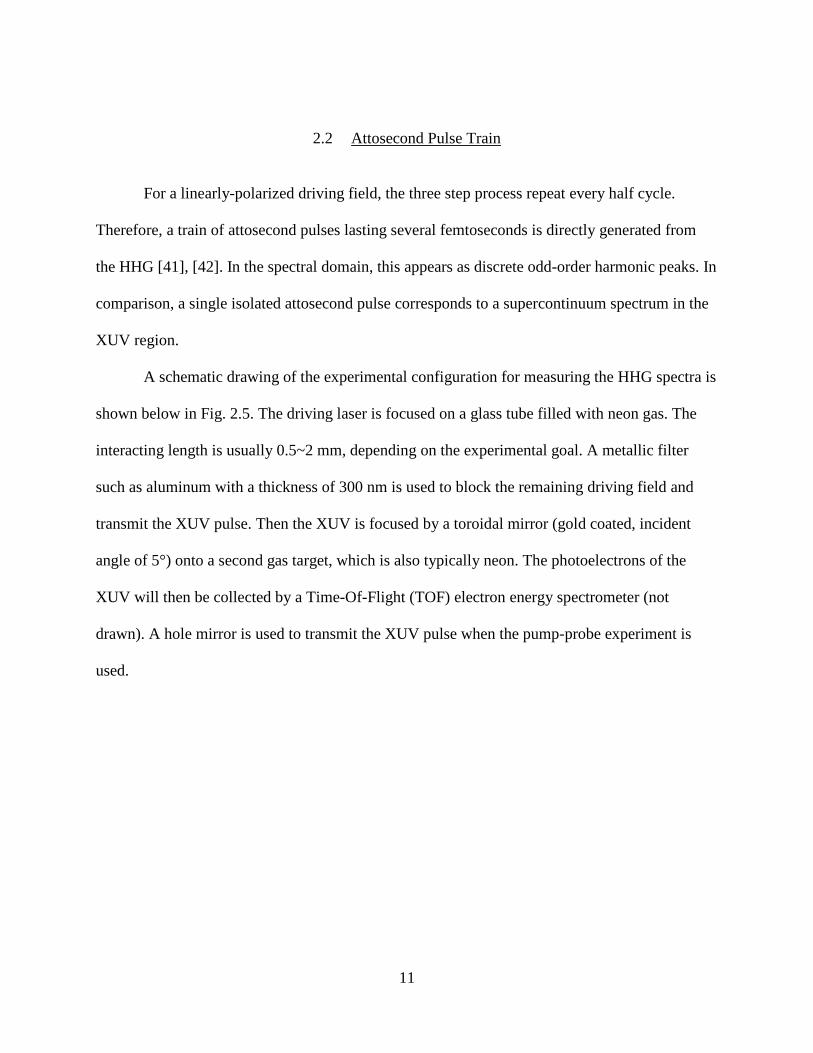
2.2 Attosecond Pulse Train
For a linearly-polarized driving field, the three step process repeat every half cycle.
Therefore, a train of attosecond pulses lasting several femtoseconds is directly generated from
the HHG [41], [42]. In the spectral domain, this appears as discrete odd-order harmonic peaks. In
comparison, a single isolated attosecond pulse corresponds to a supercontinuum spectrum in the
XUV region.
A schematic drawing of the experimental configuration for measuring the HHG spectra is
shown below in Fig. 2.5. The driving laser is focused on a glass tube filled with neon gas. The
interacting length is usually 0.5~2 mm, depending on the experimental goal. A metallic filter
such as aluminum with a thickness of 300 nm is used to block the remaining driving field and
transmit the XUV pulse. Then the XUV is focused by a toroidal mirror (gold coated, incident
angle of 5°) onto a second gas target, which is also typically neon. The photoelectrons of the
XUV will then be collected by a Time-Of-Flight (TOF) electron energy spectrometer (not
drawn). A hole mirror is used to transmit the XUV pulse when the pump-probe experiment is
used.
11

Figure 2.5 Schematic drawing of a typical experimental configuration for generating high-order harmonics and detecting photoelectron spectra.
An experimental photoelectron spectrum of attosecond pulse train is plotted in Fig. 2.6.
The driving field is the home-built Ti:Sapphire CPA laser with 1 mJ and 25 fs pulse duration.
Neon gas was used for both generation and detection. The details of the setup can be found in
Chapter 5.
12

Figure 2.6 Experimental photoelectron spectrum with linearly polarized driving laser (Ti:Sapphire laser with 1 millijoule pulse energy and 25 femtosecond pulse duration). The cutoff at about 50 eV are from Aluminum filter which was used to block the remaining driving field.
Attosecond pulse trains can be very useful in certain scenarios. However, in order to
achieve attosecond temporal resolution in pump-probe experiments, single isolated attosecond
pulses are needed. In the next chapter, three different schemes for generating single attosecond
pulse are explained and compared.
13

CHAPTER 3 ISOLATED ATTOSECOND PULSES
To obtain single isolated attosecond pulses, the three-step process can only happen once
per driving pulse. The most straightforward way is to use a driving pulse of only single-cycle
duration. This was done in Ref [7], where a 3.5 fs driving laser was used. Even with such a short
pulse, harmonic peaks can still be observed in the low photon energy region. A zirconium filter
was applied to filter out the low energy component, and only a single attosecond pulse was
transmitted. With this so-called Amplitude Gating (AG) method, 80 as isolated pulses were
generated [7]. However, the requirement of AG is extremely difficult to meet. To date, only a
few laboratories in the world have demonstrated single attosecond pulse generation with this
method. Additionally, since it filters out many low order harmonics, only the cutoff region can
contribute to the final single attosecond pulse. It significantly limits the achievable bandwidth for
the supercontinuum and hence the pulse duration, since the cutoff region is typically only a small
portion of the total high harmonic spectrum.
Another way of solving this problem is to manipulate the ellipticity of the driving electric
field. In the last step from the three-step model, the accelerated electron needs to come back and
recombine with the parent ion. If ellipticity is introduced to the driving field, the electron can be
accelerated in a transverse direction. Therefore, the possibility of recombination is greatly
reduced [43]. Experimentally, a significant drop of the HHG signal has been observed along with
increasing ellipticity of the driving laser [44]. This opens another way to generate single
attosecond pulse without needing single-cycle driving lasers. Two schemes, Polarization Gating
(PG) and Double Optical Gating (DOG), have been proposed, and both have been demonstrated
experimentally [32], [45]. The PG and DOG not only relax the requirement for the driving laser,
14

but they can also generate a supercontinuum spectra that covers even the plateau region.
Therefore, in this chapter, these two schemes (especially DOG) are explained in detail.
3.1 Few-Cycle Femtosecond Lasers
To drive the generation of isolated attosecond pulses, few-cycle femtosecond lasers,
commonly based on Ti:Sapphire, are used. Often Ti:Sapphire is chosen as the gain material due
to its long upper-state lifetime, broad gain bandwidth, and high damage threshold. Therefore, in
this work a Ti:Sapphire Chirped Pulse Amplification (CPA) system was built and a hollow-core
fiber-compressor system was applied to produce about 7 fs, 1 mJ pulse at a 1 kHz repetition rate.
A schematic drawing of the whole system is shown below in Fig. 3.1.
Figure 3.1 Schematic drawing of a Ti:Sapphire few-cycle laser system.
The mode-locked Ti:Sapphire oscillator (Femtolasers Scientific Pro) pumped by a
continuous Nd:YVO4 laser (Coherent Verdi G) at 532 nm produces the 10 fs pulses at around an
80 MHz repetition rate. The pulse energy is about 5 nJ, which is not sufficient for directly
exciting the HHG. The oscillator beam then goes through a grating pair which stretches the pulse
15

duration to ~200 ps. The stretched pulse is then amplified in two stages and reaches a pulse
energy of ~5 mJ. Then a grating pair compressor is used to compress the pulse duration to
around 25 fs and 3 mJ. The stretcher is used to avoid damaging the Ti:Sapphire crystal during
amplification. This technique was invented in early 1980s and is termed as Chirped Pulse
Amplification.
To generate isolated attosecond pulses, a few-cycle driving laser should be used. The 25
fs laser pulse from the CPA is focused into a hollow-core fiber filled with neon gas, where its
spectrum is broadened by self-phase modulation. The positive chirp of the pulses introduced by
this process is compensated by six pairs of chirped mirrors. Finally, around 1 mJ, 7 fs pulses are
produced and ready to be used as the driving field in HHG.
The pulse duration of the laser was evaluated by Second-harmonic Frequency Resolved
Optical Gating (SHG-FROG) [46]. In SHG-FROG, the input beam is split into two identical
pulses which are then recombined in a frequency-doubling crystal. The generated second
harmonic beam is then recorded by an imaging spectrometer. The recorded FROG trace is
reconstructed with a computer using the Principal Component Generalized Projections
Algorithm (PCGPA) [47].
The electric field of a pulse can be written as
𝜀𝜀(𝑡𝑡) = 𝐸𝐸(𝑡𝑡)𝐴𝐴−𝑖𝑖𝜔𝜔𝑡𝑡, ( 3.1 )
where E(t) is the complex envelope of the pulse and 𝐼𝐼 is the carrier frequency of the pulse.
Therefore, the complex envelope of the SHG-FROG signal is given by
𝐸𝐸𝐸𝐸𝐹𝐹𝐸𝐸𝐹𝐹(𝑡𝑡, 𝜏𝜏) = 𝐸𝐸(𝑡𝑡)𝐸𝐸(𝑡𝑡 − 𝜏𝜏), ( 3.2 ) where τ is the time delay between the two identical pulses. The FROG trace recorded by the
CCD detector can then be expressed as:
16

𝐼𝐼𝐸𝐸𝐹𝐹𝐸𝐸𝐹𝐹(𝐼𝐼, 𝜏𝜏) = �∫ 𝐸𝐸(𝑡𝑡)𝐸𝐸(𝑡𝑡 − 𝜏𝜏)𝐴𝐴𝑠𝑠𝐼𝐼𝑡𝑡𝑟𝑟𝑡𝑡∞−∞ �
2 ( 3.3 )
For a typical FROG, it is not necessary that two identical beams are used. So generally, a FROG
trace can be expressed as:
𝐼𝐼𝐸𝐸𝐹𝐹𝐸𝐸𝐹𝐹(𝐼𝐼, 𝜏𝜏) = �∫ 𝐸𝐸(𝑡𝑡)𝐹𝐹(𝑡𝑡)𝐴𝐴𝑠𝑠𝐼𝐼𝑡𝑡𝑟𝑟𝑡𝑡∞−∞ �
2 ( 3.4 )
𝐸𝐸(𝑡𝑡) is the electric field which needs to be characterized, and 𝐹𝐹(𝑡𝑡) is the gate function, which
could be a unknown field. The equation above is important since it will be compared with the
atto-streaking trace which is used to characterize the attosecond pulses. Details can be found in
Chapter 4.
The FROG trace for the pulse after the hollow-core fiber is shown in Fig. 3.2. The pulse duration
used to generate isolated attosecond pulses is ~7 fs, which corresponds to ~3 optical cycles.
17

Figure 3.2 The FROG measurement of a few-cycle laser pulse after the hollow-core fiber. (a) The measured FROG trace. (b) The reconstructed FROG trace. (c) The retrieved pulse shape (black dotted curve) and phase (blue dotted curve). (d) The retrieved power spectrum (black dotted curve) and phase (blue dotted line) and independently measured spectrum (red dotted curve).
3.2 Polarization Gating
After the development of the three-step model in 1993, the strong dependence of the
HHG efficiency on the ellipticity of the driving field was both theoretically treated and
experimentally demonstrated [43], [48], [49]. If the driving field is elliptical, the tunnel-ionized
electrons not only gain velocity in the z direction (which is the direction of the laser field with
linear polarization), but they also are accelerated in the transverse direction. When the electrons
18

return, the displacement in the transverse direction significantly reduces the possibility of
recombination. This effect has been experimentally observed.
The idea of PG was first proposed in 1994 by Corkum to take advantage of this ellipticity
dependence [45], suggesting using two laser pulses with different frequencies. In 1999,
Platonenko and Strelkov proposed a different method which superimposes a left- and right-
circularly polarized pulse for PG with only one central frequency [50]. This scheme has been
adopted by many researchers. In 2006, isolated 130 as pulses using PG method were
experimentally demonstrated [30].
Experimentally, PG only needs two optical devices: a full-order quartz plate and a zero-
order quarter wave plate. For a linearly-polarized laser field, the optical axis of the first full-order
quartz plate is set to be 45° versus the polarization direction of the driving field in the plane
perpendicular to the laser propagation direction. Then, due to the birefringence of the quartz
plate, the electric fields parallel and perpendicular to the optical axis travel at different velocities.
The delay between the two fields, 𝐸𝐸𝑑𝑑, is determined by the difference in the group velocities
along the ordinary and extraordinary axes as well as the thickness of the quartz plate. After that,
the zero-order quarter wave plate converts the two delayed pulses into right- and left-circularly
polarized laser. Within the temporal region where the two pulses are still overlapped, the
ellipticity is cancelled, and a linearly-polarized field is obtained. It is this region of overlap that
defines a gate period with linear polarization. All other regions are elliptically polarized and
therefore cannot generate the high order harmonics. If the gate is short enough—shorter than half
of the optical period—then only one attosecond pulse can be generated. For example: using a
Ti:Sapphire laser at a 750 nm center wavelength, the gate width should be narrower than 1.25 fs.
19

To fully understand this scheme, it is necessary to mathematically solve the final
expression of the time-varying polarized laser field. The incoming laser field can be assumed to
be a Gaussian pulse expressed as
𝐸𝐸0𝐴𝐴−2 ln(2)� 𝑡𝑡
𝜏𝜏𝑝𝑝�2
cos (𝐼𝐼0𝑡𝑡 + 𝜑𝜑𝐶𝐶𝐸𝐸) ( 3.5 )
where 𝐸𝐸0 is the peak electric field and 𝜏𝜏𝑝𝑝 is the pulse duration. After the first quartz plate (which
is a full waveplate), the two perpendicular pulses can be expressed as
𝐸𝐸𝑜𝑜(𝑡𝑡) = √22𝐸𝐸0𝐴𝐴
−2 ln(2)�𝑡𝑡−𝑇𝑇𝑑𝑑
2�𝜏𝜏𝑝𝑝
�2
cos (𝐼𝐼0𝑡𝑡 + 𝜑𝜑𝐶𝐶𝐸𝐸), ( 3.6 )
𝐸𝐸𝑒𝑒(𝑡𝑡) = √22𝐸𝐸0𝐴𝐴
−2 ln(2)�𝑡𝑡+𝑇𝑇𝑑𝑑
2�𝜏𝜏𝑝𝑝
�2
cos (𝐼𝐼0𝑡𝑡 + 𝜑𝜑𝐶𝐶𝐸𝐸) ( 3.7 )
where 𝐸𝐸𝑜𝑜(𝑡𝑡) and 𝐸𝐸𝑒𝑒(𝑡𝑡) are the ordinary and extraordinary field, 𝐸𝐸𝑑𝑑 is the delay, 𝐼𝐼0 is carrier
frequency, and 𝜑𝜑𝐶𝐶𝐸𝐸 is the carrier-envelope phase. After the zero-order quarter waveplate, the
final electric fields can be expressed as
𝐸𝐸𝑑𝑑𝑑𝑑𝑖𝑖𝑑𝑑𝑖𝑖𝑑𝑑𝑑𝑑(𝑡𝑡) = √22𝐸𝐸0 �𝐴𝐴
−2 ln(2)�𝑡𝑡−𝑇𝑇𝑑𝑑
2�𝜏𝜏𝑝𝑝
�2
+ 𝐴𝐴−2 ln(2)�
𝑡𝑡+𝑇𝑇𝑑𝑑
2�𝜏𝜏𝑝𝑝
�2
� cos(𝐼𝐼0𝑡𝑡 + 𝜑𝜑𝐶𝐶𝐸𝐸) ( 3.8 )
𝐸𝐸𝑑𝑑𝑚𝑚𝑡𝑡𝑖𝑖𝑑𝑑𝑑𝑑(𝑡𝑡) = √22𝐸𝐸0 �𝐴𝐴
−2 ln(2)�𝑡𝑡−𝑇𝑇𝑑𝑑
2�𝜏𝜏𝑝𝑝
�2
− 𝐴𝐴−2 ln(2)�
𝑡𝑡+𝑇𝑇𝑑𝑑
2�𝜏𝜏𝑝𝑝
�2
� sin(𝐼𝐼0𝑡𝑡 + 𝜑𝜑𝐶𝐶𝐸𝐸) ( 3.9 )
where 𝐸𝐸𝑑𝑑𝑑𝑑𝑖𝑖𝑑𝑑𝑒𝑒(𝑡𝑡) is along the original polarized direction and 𝐸𝐸𝑑𝑑𝑚𝑚𝑡𝑡𝑒𝑒(𝑡𝑡) is perpendicular to the
original polarized direction. Assuming a 3-cycle delay by the full-order quartz plate, the final
driving and gating fields are plotted with the red line in Fig. 3.3 (a) and (b). A 3-D plot in Fig.
20

3.4 below clearly shows that only the center portion of the final laser field is linear, while all
other portions are highly elliptical.
Figure 3.3 Schematic drawings of the (a) driving and (b) gating field for PG and DOG techniques. The blue line in the (a) driving field is the second harmonic of the gating field using only for DOG.
21

Figure 3.4 The final electric field for PG in a three dimensional frame. The black line is total field. The red (driving field) and green lines (gating field) are its projection on two orthogonal planes. The delay introduced by the first quartz plate is three cycles.
The ellipticity of the final electric field is a time-dependent function and can be calculated as
𝜉𝜉(𝑡𝑡) = 𝐸𝐸𝑔𝑔𝑔𝑔𝑡𝑡𝑔𝑔𝑔𝑔𝑔𝑔𝐸𝐸𝑑𝑑𝑑𝑑𝑔𝑔𝑑𝑑𝑔𝑔𝑔𝑔𝑔𝑔
= 1−𝑒𝑒−4 ln(2)
𝑇𝑇𝑑𝑑𝜏𝜏𝑝𝑝2 𝑡𝑡
1+𝑒𝑒−4 ln(2)
𝑇𝑇𝑑𝑑𝜏𝜏𝑝𝑝2 𝑡𝑡≈ �2 ln(2) 𝑇𝑇𝑑𝑑
𝜏𝜏𝑝𝑝2𝑡𝑡� ( 3.10 )
The ellipticity from the above equation should be less than a threshold value determined by the
experiment, meaning the efficiency of the HHG should decrease by at least one order of
magnitude with this ellipticity. Then the gate width within which the HHG can be generated is
𝛿𝛿𝑡𝑡𝐺𝐺 ≈𝜉𝜉𝑡𝑡ℎln (2)
𝜏𝜏𝑝𝑝2
𝑇𝑇𝑑𝑑 ( 3.11 )
where 𝜉𝜉𝑡𝑡ℎ is the threshold ellipticity for harmonic generation. To generate a single isolated
attosecond pulse, the gate width should be less than the half cycle period of the driving field. In
22

our case, a Ti:Sapphire laser system is used and this value should be 1.2 fs. As 𝜉𝜉𝑡𝑡ℎ is ~0.2 for this
wavelength, the equation becomes
𝛿𝛿𝑡𝑡𝐺𝐺 ≈0.2ln(2)
𝜏𝜏𝑝𝑝2
𝑇𝑇𝑑𝑑< 1.2 𝑓𝑓𝑠𝑠 ( 3.12 )
The benefit of PG versus AG is that we can always adjust 𝐸𝐸𝑑𝑑 to meet the requirement in
equation 3.8. The required delay 𝐸𝐸𝑑𝑑 as a function of the input laser pulse duration is shown in
Fig. 3.5 (a). It can be seen that we can maintain a gate width less than half the laser cycle, even
with a very long pulse, if the delay is properly chosen. On the other hand, the delay will also
decrease the peak intensity where the high-order harmonics are generated. As shown in Fig. 3.5
(b), the larger the delay is, the smaller the peak intensity becomes. Obviously, higher peak
intensity is preferred for a broader XUV bandwidth, smaller intrinsic chirp, and thus shorter
pulse duration. Therefore, there is a tradeoff between the two factors, and the delay should be
chosen to be as small as possible while still satisfying equation 3.8.
In addition to the gate width, another necessary condition for HHG is that the target atom
responsible for attosecond light emission must not be fully ionized when the electric field inside
the gate arrives. With the ADK model [51], the ionization probability of neon atoms can be
calculated as a function of the peak intensity inside the gate. One such result for input pulse
duration of 7 fs is shown with the black line in Fig. 3.6. According to the plot, the highest peak
intensity achievable with neon gas for a 7 fs driving pulse is 7 × 10¹⁴𝑊𝑊/𝑐𝑐𝜇𝜇2, corresponding to
a cutoff photon energy of 150 eV. Using argon, which has a smaller ionization potential, this
value is significantly reduced to 60 eV, meaning the shortest pulse duration achievable is only
~200 as. To generate shorter attosecond pulses, shorter driving pulses are needed. For example,
in Ref [30], 5 fs driving pulses were used, and isolated 130 as pulses were demonstrated.
23

However, using atoms with higher ionization potential such as helium decreases the HHG
efficiency by at least two orders of magnitude, leading to the practical difficulties in collecting
experimental data. This is why neon gas was the most suitable target atom for this work.
Figure 3.5 (a) Delay of the first quartz plate required for generating single attosecond pulses as a function of the driving pulse duration. Black: PG. Red: DOG. (b) The peak intensity inside of the gate, assuming the peak intensity of the linearly polarized input pulse is 2 × 10¹⁵𝑊𝑊/𝑐𝑐𝜇𝜇2. Black: PG. Red: DOG.
24

Figure 3.6 The ionization probabilities of a neon atom, calculated with the ADK model, as a function of the peak intensity inside the gate. The pulse duration is assumed to be 7 fs, and the gate width is calculated for PG and DOG to select a single attosecond pulse. Black line: PG. Red line: DOG It should be noted that the experimentally-measured spectral bandwidth is usually much
narrower than the calculation due to phase mismatching. Up to now it has not been demonstrated
that PG can generate single attosecond pulses with durations of less than 100 as.
3.3 Double Optical Gating
As discussed in the PG section, the gate width should be less than the half-cycle period of
the driving laser since the three steps for generating high-order harmonics repeat every half
25

cycle. If this periodicity increases to one full cycle, the requirement of the gate width is loosened
by a factor of two. This is the idea of the Double Optical Gating [31]–[33].
It is well known that by adding a second harmonic to the driving field, the field symmetry
is broken, and only one XUV pulse can be produced within one optical cycle of the driving field.
This is termed as “two-color gating”. The DOG method takes advantage of two-color gating and
combines it with the PG scheme. Since the driving field is the field actually responsible for
harmonic generation, the two-color field should also be superimposed in the same direction.
Therefore, the gating field is used to generate its second harmonic through a β-BaB2O4 (BBO)
crystal optimized for type-I phase matching. A schematic drawing of the two color field is
plotted with the blue line in Fig. 3.3 (a).
Experimentally it is simple to achieve DOG conditions. Instead of using a zero-order
quarter waveplate, another full-order quartz plate and a BBO combine and function as the quarter
waveplate. The typical experimental photoelectron spectra with linear and DOG driving fields
are plotted in Fig. 3.7. The details of the setup can be found in Chapter 5. The sharp edge at 52
eV is from the 300 nm thick aluminum filter which is used to block the remaining driving pulse
while transmitting the XUV light.
Compared to PG, the most obvious advantage of the DOG technique is that longer
driving pulses are allowed for single attosecond pulse generation, as shown in Fig. 3.5 (a). This
is very critical since PG practically requires 5 fs driving pulse, which, while not impossible, is
still quite a challenge. This is because a longer driving pulse requires a larger delay, which
reduces the peak intensity. In contrast, DOG allows for 7-10 fs driving pulses while still
generating a strong signal and high HHG cutoff. Such pulse durations can be routinely produced
from the hollow core fiber and compressor system.
26

Figure 3.7 The photoelectron spectra of HHG generated with linear polarized driving laser (black line) and DOG driving laser (red line). The 300 nm thick Aluminum filter is used to block the remaining driving pulse and transmitting the XUV.
Furthermore, DOG can be appreciated from another point of view: for equal pulse
durations, DOG allows the use of less delay time 𝐸𝐸𝑑𝑑 compared to PG, hence increasing the peak
intensity inside the gate with the same pulse energy (as shown in Fig. 3.5 (b) with the red curve).
More importantly, the shorter delay time required by DOG significantly reduces the ionization
before the gate under the same peak intensity (as calculated by the ADK model and shown in the
red curve in the Fig. 3.6). In other words, this calculation shows that higher peak intensity inside
the gate can be used for DOG than PG, which is crucial for generating a broadband
supercontinuum from HHG.
Since DOG is much better than PG, it is applied throughout the work shown in this
dissertation. Experimental results are presented in Chapter 5 and 6.
27

CHAPTER 4 TEMPORAL CHARACTERIZATION OF ATTOSECOND PULSES
To characterize femtosecond pulses, FROG is often used, as discussed in Chapter 3.1.
However, using FROG to measure attosecond pulses is difficult due to low photon fluxes. Since
the spectra of the attosecond pulses can be easily measured, only the spectral phase information
is needed for complete characterization. Currently, the technique used for measuring the spectral
phase is termed as “attosecond streaking”, which is similar to the concept of FROG for
measuring the spectral phase of the femtosecond laser. It should be noted that with attosecond
pulses today, the electric fields of the femtosecond lasers can be directly mapped out without any
ambiguity in the attosecond streaking experiments [52]. In this section, a simple technique to
characterize the attosecond pulse train termed as Reconstruction of attosecond beating by
interference of two-photon transition (RABITT) was first introduced. Then the principle of the
attosecond streaking technique for measuring the spectral phase for isolated attosecond pulses
was discussed, and two algorithms to retrieve the phase are discussed and compared.
4.1 RABITT
Reconstruction of attosecond beating by interference of two-photon transition (RABITT)
was developed for characterizing the average duration of the attosecond pulses in a train
generated from the HHG. In the spectrum domain, the attosecond pulse train corresponds to
discrete harmonic peaks separated by two photon energies of the driving laser. The power
28

spectrum can be easily measured with an electron TOF spectrometer as shown in Fig. 2.6. A
typical experimental configuration can be found in Fig 2.5.
To characterize the attosecond pulse duration, only the phase information is needed. In
RABITT, in addition to the XUV attosecond train, an extra weak IR laser is introduced in the
detection. Due to the laser symmetry, only the odd order harmonic can be observed for the HHG.
In the detection, a ground state electron inside the atom of a target gas (i.e. Neon atom) is
photoionized by the XUV pulse. With the presence of the extra IR laser, it is possible to
photoionize ground state electron to a continuum state between two harmonic. This is called the
“sideband”, which is the transition caused by one XUV and one IR photon, as shown in Fig. 4.1
below. The electron in the ground state can absorb an XUV photon 𝐸𝐸𝑞𝑞−1𝐴𝐴𝑖𝑖(𝑞𝑞−1)𝜔𝜔𝑡𝑡+∅𝑞𝑞−1 and an
IR photon 𝐸𝐸1𝐴𝐴𝑖𝑖𝜔𝜔𝑡𝑡 or absorb an XUV photon 𝐸𝐸𝑞𝑞−1𝐴𝐴𝑖𝑖(𝑞𝑞+1)𝜔𝜔𝑡𝑡+∅𝑞𝑞+1 and emit an IR photon 𝐸𝐸1𝐴𝐴𝑖𝑖𝜔𝜔𝑡𝑡.
So the final sideband can be expressed as (assuming the intensity of each harmonic peak is the
same)
𝑏𝑏𝑠𝑠𝑖𝑖𝑑𝑑𝑒𝑒𝑠𝑠𝑚𝑚𝑑𝑑𝑑𝑑 (𝐼𝐼, 𝜏𝜏) ∝ ∫ (𝐸𝐸𝑞𝑞−1𝐸𝐸1𝐴𝐴𝑖𝑖𝑞𝑞𝜔𝜔𝑡𝑡+∅𝑞𝑞−1 + 𝐸𝐸𝑞𝑞+1𝐸𝐸1𝐴𝐴𝑖𝑖𝑞𝑞𝜔𝜔𝑡𝑡+∅𝑞𝑞+1)∞−∞ 𝐴𝐴−𝑖𝑖𝜔𝜔𝑡𝑡𝑟𝑟𝑡𝑡 ( 4.1 )
The 𝜏𝜏is the delay between the XUV and the IR. As the delay is scanned, the intensity of the
sideband in the spectrum domain can be expressed as
𝐼𝐼𝑠𝑠𝑠𝑠𝑟𝑟𝐴𝐴𝑏𝑏𝑟𝑟𝑠𝑠𝑟𝑟(𝐼𝐼, 𝜏𝜏) ∝ �∫ �𝐸𝐸𝑞𝑞−1𝐸𝐸1𝐴𝐴𝑠𝑠𝑞𝑞𝐼𝐼𝑡𝑡+∅𝑞𝑞−1 + 𝐸𝐸𝑞𝑞+1𝐸𝐸1𝐴𝐴𝑠𝑠𝑞𝑞𝐼𝐼𝑡𝑡+∅𝑞𝑞+1�∞−∞ 𝐴𝐴−𝑠𝑠𝐼𝐼𝑡𝑡𝑟𝑟𝑡𝑡�
2∝ [1 +
cos (2𝐼𝐼𝜏𝜏 + ∅𝑞𝑞+1 − ∅𝑞𝑞−1)] ( 4.2 ) It can be seen that the intensity of the sideband is oscillating depending on the spectral phase
difference ∅𝑞𝑞+1 − ∅𝑞𝑞−1. Therefore the relative temporal position of each sideband determine the
spectral phase difference between each adjacent harmonics from the HHG.
29

Figure 4.1 A schematic drawing of the RABITT photon transition. The sideband (dashed line) can be produced by one XUV photon adding one IR photon.
30

4.2 The Principle of Attosecond Streaking
To characterize the isolated attosecond pulse, RABITT cannot be used since the spectra
now are continuous. To solve this issue, the attosecond streaking can be used.Traditionally
speaking, a streak camera is a device used to streak the fast electron pulses by applying a fast-
varying high voltage perpendicular to the electron propagation direction [53]. The streaked
electrons are spatially displaced depending on their experience in the fast-varying voltage. This
way, the temporal information of the electrons can be obtained from their spatial distribution.
The resolution of a streak camera is determined by the streaking speed (if the instrumental
resolution is infinitely small). In other words, the gradient of this fast-varying sweeping voltage
will determine the resolution. For measuring attosecond pulse, there is no such device that can
supply a sweeping voltage on the attosecond scale. However, the fast-varying electric field of a
laser which is phase-locked with the attosecond pulse can be used as the “sweeping voltage”.
This is the basic idea of the attosecond streaking [54], [55]. Practically, this phase-locked
streaking pulse usually comes from a small portion of the driving laser itself. To completely
understand this process, quantum mechanics should be applied [56], [57].
As shown in Fig. 4.2 (a), the photoelectrons generated by the XUV pulse are dressed by
the streaking field, and their momentum is altered. By scanning the delay between the XUV and
the streaking field in Fig. 4.2 (a), a two-dimensional spectrogram can be obtained, as plotted in
Fig. 4.2 (b). This so-called “streaking trace” contains the complete information for
characterization.
31

Figure 4.2 A schematic drawing depicting the principle of attosecond streaking (a) XUV (blue) and streaking field (red dashed) (b) The streaking trace obtained by scanning the delay between XUV and streaking field and recording photoelectron spectra at each delay.
32

4.3 Complete Reconstruction of Attosecond Bursts
In a streaking experiment, the attosecond XUV pulse is focused onto a gaseous target to
photoionize the neutral atoms. The photoelectrons generated are then streaked by a phase-locked
few-cycle intense IR laser field, giving a momentum shift to the electrons. Assuming a linear
streaking field is applied, the momentum change can be expressed as [54], [58]
Δ𝑝𝑝(𝑡𝑡) = ∫ 𝐴𝐴𝜀𝜀(𝑡𝑡′)𝑟𝑟𝑡𝑡′∞𝑡𝑡 = 𝐴𝐴𝐴𝐴𝐿𝐿(𝑡𝑡) ( 4.3 )
where 𝐴𝐴𝐿𝐿(𝑡𝑡) is the vector potential of the laser field. This momentum shift can be recorded as a
function of delay between the XUV pulse and the streaking field by a Time-Of-Flight (TOF)
electron spectrometer. In atomic units, the final streaking trace can be expressed as a function of
energy and delay as
𝑆𝑆(𝑊𝑊, 𝜏𝜏𝐷𝐷) ≈ �∫ 𝑟𝑟𝑡𝑡𝐸𝐸𝑋𝑋(𝑡𝑡 − 𝜏𝜏)∞−∞ 𝑟𝑟[𝑝𝑝 + 𝐴𝐴𝐿𝐿(𝑡𝑡)]𝐴𝐴𝑖𝑖𝑖𝑖(𝑝𝑝,𝑡𝑡)𝐴𝐴−𝑖𝑖�𝑊𝑊+𝐼𝐼𝑝𝑝�𝑡𝑡�
2 ( 4.4 )
𝜑𝜑(𝑝𝑝, 𝑡𝑡) = −∫ 𝑟𝑟𝑡𝑡′�𝑝𝑝𝐴𝐴𝐿𝐿(𝑡𝑡′) cos 𝜃𝜃 + 𝐴𝐴𝐿𝐿2(𝑡𝑡′) 2⁄ �∞𝑡𝑡 ( 4.5 )
where 𝐸𝐸𝑋𝑋 is the complex field amplitude of the XUV pulse, 𝜏𝜏 is the delay between the XUV and
streaking pulses, 𝑊𝑊 is the kinetic energy of the photoelectron, and Ip is the ionization potential of
the target gas. For a narrow bandwidth XUV spectrum, we can replace the momentum in
equation 4.3 with the central momentum 𝑝𝑝0 and the dipole transition element 𝑟𝑟(𝑝𝑝) with a
constant 𝑟𝑟0. This condition is called the Central Momentum Approximation (CMA). Under the
CMA, we rewrite equation 4.3 to be
𝑆𝑆(𝑊𝑊, 𝜏𝜏𝐷𝐷) ∝ �∫ 𝑟𝑟𝑡𝑡𝐸𝐸𝑋𝑋(𝑡𝑡 − 𝜏𝜏)∞−∞ 𝐹𝐹 (𝑡𝑡)𝐴𝐴−𝑖𝑖�𝑊𝑊+𝐼𝐼𝑝𝑝�𝑡𝑡�
2 ( 4.6 )
33

Assuming only electrons parallel to the streaking field are detected, the gating function 𝐹𝐹(𝑡𝑡) can
be expressed as:
𝐹𝐹(𝑡𝑡) = exp {−𝑠𝑠 ∫ 𝑟𝑟𝑡𝑡′�𝑝𝑝0𝐴𝐴𝐿𝐿(𝑡𝑡′) + 𝐴𝐴𝐿𝐿2(𝑡𝑡′) 2⁄ �∞𝑡𝑡 }. ( 4.7 )
Note that 𝐹𝐹(𝑡𝑡) is a function of time but independent of the momentum. It can be seen that
Equation 4.4 has the same form as the Equation 3.4, which is used in Frequency-Resolved
Optical Gating (FROG) to characterize the femtosecond laser pulse. The phase modulation
function 𝐹𝐹(𝑡𝑡) works as a temporal gate (using FROG terminology). The streaking trace can then
be treated as a FROG trace and both 𝐸𝐸𝑋𝑋(𝑡𝑡 − 𝜏𝜏) and 𝐹𝐹 (𝑡𝑡) can be retrieved using the well-known
Principal Component Generalized Projections Algorithm (PCGPA) [47], [59], [60]. This
technique is termed as the Complete Reconstruction of Attosecond Bursts (CRAB) [58].
PCGPA is very robust against noise [59]. However, the CMA must be obeyed for CRAB
to perform correctly. When an ultrabroadband continuum is generated and its spectral phase
needs to be retrieved, the CRAB method does not work properly. In this case, a new technique
for phase retrieval without the CMA is necessary.
4.4 Phase Retrieval by Omega Oscillation Filtering
As explained in the above section, a streaking trace collects the oscillations of the
photoelectron spectra as the delay between the XUV and streaking IR pulses is altered. However,
in the limit of low streaking intensity, similar to the RABITT, this oscillation can also be
interpreted as the interference of different quantum paths to the same final electron state [61].
Mathematically speaking, the gate function can be rewritten as follows:
34

𝐹𝐹(𝑡𝑡) = 𝐴𝐴𝑖𝑖𝑖𝑖(𝑡𝑡) ≈ 1 + 𝑠𝑠𝑖𝑖(𝑡𝑡) ( 4.8 )
In the lower limit the of the streaking field, 𝑖𝑖(𝑡𝑡) can be estimated by
𝑖𝑖(𝑡𝑡) ≈�8𝑊𝑊𝑈𝑈𝑝𝑝(𝑡𝑡)
𝜔𝜔𝐿𝐿cos 𝜃𝜃 cos(𝐼𝐼𝐿𝐿𝑡𝑡) =
�8𝑊𝑊𝑈𝑈𝑝𝑝(𝑡𝑡)
2𝜔𝜔𝐿𝐿cos 𝜃𝜃 (𝐴𝐴𝑖𝑖𝜔𝜔𝐿𝐿𝑡𝑡 + 𝐴𝐴−𝑖𝑖𝜔𝜔𝐿𝐿𝑡𝑡) ( 4.9 )
where 𝑈𝑈𝑝𝑝 is the ponderomotive energy and 𝐼𝐼𝐿𝐿 is the angular frequency of the streaking field.
Plugging this into equation 4.4 yields [61]
𝑆𝑆(𝑊𝑊, 𝜏𝜏𝐷𝐷) = �∫ 𝑟𝑟𝑡𝑡𝐸𝐸𝑋𝑋(𝑡𝑡 − 𝜏𝜏)∞−∞ 𝐹𝐹 (𝑡𝑡)𝐴𝐴−𝑖𝑖�𝑊𝑊+𝐼𝐼𝑝𝑝�𝑡𝑡�
2≈ 𝑆𝑆0 + 𝑆𝑆𝜔𝜔𝐿𝐿 + 𝑆𝑆2𝜔𝜔𝐿𝐿. ( 4.10 )
where 𝑆𝑆0, 𝑆𝑆𝜔𝜔𝐿𝐿, 𝑆𝑆2𝜔𝜔𝐿𝐿 are streaking trace components which oscillate with DC, one dressing laser
frequency, and two dressing laser frequencies. Higher-order components are ignored here. The
trace 𝑆𝑆𝜔𝜔𝐿𝐿 contains the complete information of the XUV pulse. To retrieve the spectral phase
difference, it is only needed to guess the spectral phase that matches𝑆𝑆𝜔𝜔𝐿𝐿. Retrieving the spectral
phase from these oscillations then reduces to a minimization problem.
Unlike FROG-CRAB, the PROOF method does not use FROG phase retrieval
algorithms, and the central momentum approximation is not needed. Furthermore, observation of
this oscillation does not require high streaking intensities, as only one NIR photon is needed to
couple the continuum states. This has a significant advantage since the strong streaking field can
also photoionize the target gas. Similar to HHG, the electric field first tunnel ionizes the ground
state electron, then this electron is accelerated in the remaining laser field. Under certain
circumstances (see equation 2.4 and related discussion), this accelerated electrons can come back
to the parent ion. However, instead of recombining with the ion like in HHG, it is scattered
35

away. This process of generating free electrons is termed as Above Threshold Ionization (ATI).
Obviously, the lower intensities can reduce the electron noise from the ATI significantly.
To understand the PROOF from a physical standpoint: for low streaking intensities, one
can interpret the streaking as the interference of electrons ionized through different pathways. As
explained in Ref [61], the electron signal at a given energy may come from direct ionization
from one XUV photon, one XUV plus one IR photon, and one XUV minus one IR photon.
Therefore, when the component of oscillation with the dressing laser center frequency 𝐼𝐼𝐿𝐿 is
extracted, the phase angle of the sinusoidal oscillation 𝛼𝛼(𝐼𝐼) is related to the spectral phases
φ(𝐼𝐼𝑑𝑑 − 𝐼𝐼𝐿𝐿 ), φ(𝐼𝐼𝑑𝑑), and φ(𝐼𝐼𝑑𝑑 + 𝐼𝐼𝐿𝐿 ) of the three XUV frequency components separated by one
laser photon energy and the intensities I(𝐼𝐼𝑑𝑑 − 𝐼𝐼𝐿𝐿 ), I(𝐼𝐼𝑑𝑑 + 𝐼𝐼𝐿𝐿):
tan[𝛼𝛼(𝐼𝐼)] = �𝐼𝐼(𝜔𝜔𝑑𝑑+𝜔𝜔𝐿𝐿)sin[𝑖𝑖(𝜔𝜔𝑑𝑑)−𝑖𝑖(𝜔𝜔𝑑𝑑+𝜔𝜔𝐿𝐿)]−�𝐼𝐼(𝜔𝜔𝑑𝑑−𝜔𝜔𝐿𝐿)sin[𝑖𝑖(𝜔𝜔𝑑𝑑−𝜔𝜔𝐿𝐿)−𝑖𝑖(𝜔𝜔𝑑𝑑)]�𝐼𝐼(𝜔𝜔𝑑𝑑+𝜔𝜔𝐿𝐿)cos[𝑖𝑖(𝜔𝜔𝑑𝑑)−𝑖𝑖(𝜔𝜔𝑑𝑑+𝜔𝜔𝐿𝐿)]−�𝐼𝐼(𝜔𝜔𝑑𝑑−𝜔𝜔𝐿𝐿)cos[𝑖𝑖(𝜔𝜔𝑑𝑑−𝜔𝜔𝐿𝐿)−𝑖𝑖(𝜔𝜔𝑑𝑑)]
( 4.11 )
The equation can be understood as the interference between the single-photon (XUV only) and
two-photon (XUV plus NIR) transitions from the atomic ground state to the continuum state
𝐼𝐼𝑑𝑑 − 𝐼𝐼𝑝𝑝.
Initially, the PROOF algorithm was written to minimize only the difference between the
experimental phase angle and the guessed one. However, the robustness against many practical
parameters was untested. In contrast, the PCGPA algorithm applied in the CRAB method has
been demonstrated to be very robust against noise and other imperfections. Therefore, it would
be ideal to use the PCGPA algorithm in the PROOF. Since the spectral and phase information
are completely encoded in 𝑆𝑆𝜔𝜔𝐿𝐿(𝐼𝐼, 𝜏𝜏), we intentionally construct a new streaking trace termed as
PROOF trace, 𝑆𝑆𝑃𝑃𝑃𝑃𝑃𝑃𝑃𝑃𝑂𝑂(𝐼𝐼, 𝜏𝜏𝐷𝐷) = 𝑆𝑆0 + 𝑑𝑑0𝑑𝑑𝑆𝑆𝜔𝜔𝐿𝐿 + 𝑑𝑑02
𝑑𝑑2𝑆𝑆2𝜔𝜔𝐿𝐿, in which the phase gate function is
36

independent of the momentum. Therefore, PCGPA can directly work on the PROOF trace
without the central momentum approximation. This way, we take advantage of the robustness of
the PCGPA while still avoiding the CMA. This method has been applied in retrieving the single
67 as pulse.
4.5 Reconstruction Error
Since the FROG was first introduced during the early 1990’s for femtosecond laser
characterization, there is a fundamental question needs to ask: how accurate is the phase retrieval
of the PCGPA program? To answer this question, the FROG error, a criterion for describing if
FROG algorithm converges successfully, was proposed [46]. The FROG error can be expressed
as [62]:
𝜖𝜖𝑂𝑂𝑃𝑃𝑃𝑃𝐺𝐺 = � 1𝑁𝑁2∑ ∑ �𝐼𝐼(𝐼𝐼𝑖𝑖, 𝜏𝜏𝑗𝑗) − 𝐼𝐼′(𝐼𝐼𝑖𝑖, 𝜏𝜏𝑗𝑗)�
2𝑁𝑁𝑗𝑗=1
𝑁𝑁𝑖𝑖=1 �
1/2 ( 4.12 )
where N is the pixel number of the spectrogram, 𝐼𝐼(𝐼𝐼𝑖𝑖, 𝜏𝜏𝑗𝑗) and 𝐼𝐼′(𝐼𝐼𝑖𝑖, 𝜏𝜏𝑗𝑗) are the (i, j) component
in the experimental and retrieved trace. Extensive tests have been done to determine the value of
the 𝜖𝜖𝑂𝑂𝑃𝑃𝑃𝑃𝐺𝐺 when the retrieval is considered converged. Since there is only one converging
solution for the FROG, the convergence leads to the correct phase retrieval.
When the FROG idea was further applied in attosecond regime at 2005, considering the
similarity between a streaking trace and a FROG trace with a pure phase gate, it seems natural to
follow the FROG error criterion in the attosecond region. However we noticed that the FROG
error is often used in the case with a real gate function such as Polarization Gating and Second
Harmonic Gating. For an attosecond streaking measurement, it actually has a gating function
37

with only a phase term 𝐴𝐴𝑖𝑖𝑖𝑖(𝑡𝑡). From the analysis in the section above, the zero-order component
of the streaking trace 𝐼𝐼0, while the largest component in the spectrogram, does not contain any
XUV phase information of the XUV pulse since it does not oscillating with time delay τ. This
suggests the largest contribution of the FROG error, which is inherited from the DC component
of the streaking trace, does not reflect the accuracy of the reconstruction either. The main term
containing the XUV phase information is the one oscillating with one IR laser frequency, so it is
apparent that we should use a similar expression but replace the whole streaking trace with only
the one 𝐼𝐼𝐿𝐿 term. The PROOF error can be therefore expressed as:
𝜖𝜖𝑂𝑂𝑃𝑃𝑃𝑃𝐺𝐺 = � 1𝑁𝑁2∑ ∑ �𝐼𝐼𝜔𝜔𝐿𝐿(𝐼𝐼𝑖𝑖, 𝜏𝜏𝑗𝑗) − 𝐼𝐼′𝜔𝜔𝐿𝐿(𝐼𝐼𝑖𝑖, 𝜏𝜏𝑗𝑗)�
2𝑁𝑁𝑗𝑗=1
𝑁𝑁𝑖𝑖=1 �
1/2 ( 4.13 )
where 𝐼𝐼𝜔𝜔𝐿𝐿(𝐼𝐼𝑖𝑖, 𝜏𝜏𝑗𝑗) is the (i, j) component in the one 𝐼𝐼𝐿𝐿 trace extracted from the new built
spectrogram 𝐼𝐼𝑃𝑃𝑃𝑃𝑃𝑃𝑃𝑃𝑂𝑂(𝐼𝐼, 𝜏𝜏𝐷𝐷) and 𝐼𝐼′𝜔𝜔𝐿𝐿(𝐼𝐼𝑖𝑖, 𝜏𝜏𝑗𝑗) is the reconstructed one.
38

CHAPTER 5 EXPERIMENTAL CONFIGURATION
A broadband supercontinuum supporting single attosecond pulse can be generated with
DOG and characterized by CRAB and PROOF. To experimentally demonstrate it, an attosecond
streak camera was built based on Magnetic Bottle Energy Spectrometer (MBES). MBES is
chosen to record the photoelectron generated by the attosecond XUV pulse because of its high
resolution and collection efficiency. In this chapter, we first introduce the experimental
configuration. Then in the second section, we focus on the MBES and explain its principle and
present some simulated results. The resolution of the whole system is discussed at the end.
5.1 Experimental Configuration
A schematic drawing of the experimental configuration for the attosecond streaking
experiment is shown in Fig. 5.1. Laser pulses with 25 fs duration and 1 kHz repetition rate are
produced by a Ti:Sapphire multi-pass CPA system centered at 780 nm. The laser from the
amplifier is then focused onto a hollow-core fiber filled with neon gas. The spectral bandwidth is
expanded by self-phase modulation, and six pairs of chirped-mirrors compress the fiber output
pulse to around 7 fs in duration. This compressed beam is then split into two arms by a
broadband beam splitter. The transmitted beam (containing 90% of the total energy) propagates
through the DOG optics and is focused to a neon gas target for generation of the isolated
attosecond pulses. The reflected arm (containing the other 10% of the pulse energy) is phase-
locked to the generation beam using a stabilized interferometer (as shown by the green beam
following the same path) and recombines with the XUV pulses by a hole-drilled mirror.
39

Figure 5.1 A schematic drawing of the experimental configuration for the attosecond streaking experiment based on a Magnetic Bottle Energy Spectrometer (MBES). BS: Beam Splitter; QP: Quartz Plate; M: Silver Mirror; CM1: convex mirror with -150 mm focal length, CM2: concave mirror with 250 mm focal length; GC: Gas Cell; MF: Metallic Filter; TM: Toroidal Mirror; FM: Flat Mirror; L: Focus Lens; HM: Hole drilled Mirror; MBES: Magnetic Bottle Electron Energy Spectrometer.
The laser field in the generation arm goes through the DOG optics (QP1 and QP2) and is
focused by a convex (f = -150 mm) and a concave mirror (f = 250 mm). The effective focal
length equals to 175 mm. Then the focusing beam passes through a BBO crystal with a thickness
of 141 μm, which forms a zero-order quarter wave plate with the second quartz plate. A 0.5~1
mm-thick glass cell is positioned roughly 1 mm after the laser focal spot to ensure good phase
matching of the HHG. After that, a thin film metal filter (usually aluminum or zirconium) is used
to block the remaining driving pulse while transmitting the XUV light, which is then focused by
a gold-coated toroidal mirror onto the second gas target for photoionization. In the reflected arm,
the streaking beam passes through the exact optical path length and is focused by a 300 mm focal
lens onto the same spatial spot as the XUV beam. The photoelectron generated by the XUV
40

pulse will be momentum-shifted by the streaking field and then collected by a Magnetic-Bottle
Energy Spectrometer (MBES).
The chosen focal length and the distance between the BBO and the gas cell are related to
each other and crucial to the success of the DOG. The laser should be tightly focused on to the
gas target for high HHG cutoff. However, using mirrors unavoidably introduces astigmatism to
the focal spot. Tighter focus means larger astigmatism. Additionally, the highest peak intensity
that DOG can take for neon gas before fully depleting the ground state electrons is about 2 ×
1015 𝑊𝑊/𝑐𝑐𝜇𝜇2 , as shown in Fig. 3.7. Considering the pulse energy of the driving beam is about
0.8 mJ, the beam size needed to reach this intensity is roughly around 20 𝜇𝜇𝜇𝜇. Therefore, the
focal length is chosen to be around 150 mm to 200 mm. This sets a limitation for the distance
between the BBO and the gas cell. Also the beam size of the driving laser on BBO needs to be
small so that the intensity is high enough to produce sufficient second harmonic for the two-color
gating. On the other hand, the intensity cannot be too high without damaging the BBO. The
distance between the BBO and the gas cell is experimentally determined to satisfy the two
requirements above. The beam size is usually about 4 mm on the BBO.
Since the second harmonic and the fundamental beam have different refractive indices in
air, it is necessary to keep the BBO under the vacuum so the second harmonic and the
fundamental driving pulses are temporally overlapped on the gas target. If the focusing optics are
outside the vacuum chamber, two curved mirrors such as the systems shown in our experimental
configuration Fig. 5.1 need to be used to reduce the astigmatism. If the focusing optics can be put
inside the vacuum, such as in Ref [34], one single concave mirror can be used. However, this
type of system is complicated to construct and difficult to align. Alternatively, a focusing lens
41

could be used with easy operation. The lens configuration was first considered to destroy the
few-cycle pulses at the focus, but exact calculation showed that laser pulses as short as 5 fs can
still be obtained under certain conditions using the lens focusing. This is discussed in Chapter 7.
In the streaking experiment, the delay between the XUV and the streaking arm needs to
be stabilized during each delay step. To achieve this, an independent continuous laser centered at
532 nm follows the same path as the IR laser after the beam splitter and recombines after the
hole mirror, where an interference pattern is generated. The 532 nm wavelength is used to
separate itself with the driving laser, which usually cover the spectra from 600 nm to 900 nm.
The fringe of the interference is used to stabilize the time jitter between the XUV and streaking
arms, and about 20 as RMS stability can be obtained [63]. Simulations have been done to ensure
this level of time jitter can be tolerated for accurate reconstruction of the streaking trace [64],
[65]. The delay between the XUV and streaking beams as well as the stabilization are both
controlled by a piezo-transducer (PZT) attached to one of the flat silver mirrors in the streaking
arm, as shown in Fig. 5.1.
The Magnetic-Bottle (MB) TOF spectrometer has many advantages over the traditional
TOF spectrometers [66]. Firstly, the MBES can collect larger than 2π solid angle, leading to a
collection efficiency of over 50%. This is considerably higher than field-free spectrometers.
Since the conversion efficiency of the HHG is rather low and the energy of the generated XUV
pulse is on the order of only one nanojoule, the count rates of electrons are low. Therefore, it is
important to collect as many electrons as possible (although in attosecond streaking, electrons
with emission angle larger than 90° have opposite streaking direction and are therefore highly
undesirable). Secondly, a reasonably high resolution can be obtained if the MBES is properly
designed and a long flight tube is adapted [66]–[71]. Note that in MBES, the flight tube length
42
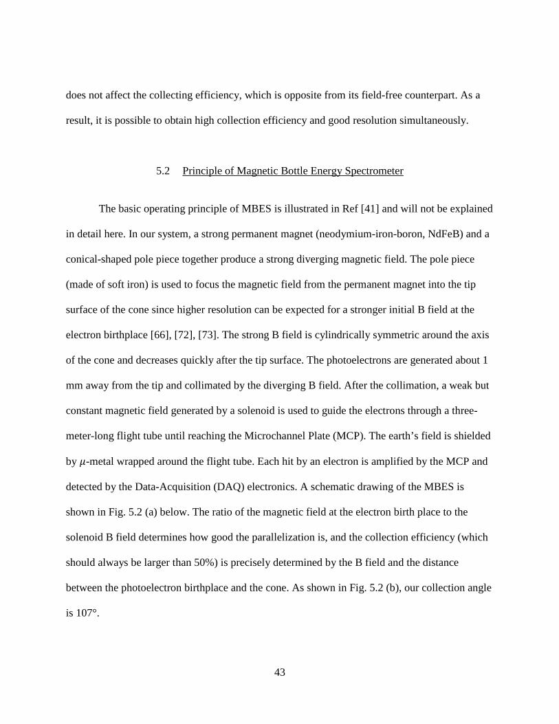
does not affect the collecting efficiency, which is opposite from its field-free counterpart. As a
result, it is possible to obtain high collection efficiency and good resolution simultaneously.
5.2 Principle of Magnetic Bottle Energy Spectrometer
The basic operating principle of MBES is illustrated in Ref [41] and will not be explained
in detail here. In our system, a strong permanent magnet (neodymium-iron-boron, NdFeB) and a
conical-shaped pole piece together produce a strong diverging magnetic field. The pole piece
(made of soft iron) is used to focus the magnetic field from the permanent magnet into the tip
surface of the cone since higher resolution can be expected for a stronger initial B field at the
electron birthplace [66], [72], [73]. The strong B field is cylindrically symmetric around the axis
of the cone and decreases quickly after the tip surface. The photoelectrons are generated about 1
mm away from the tip and collimated by the diverging B field. After the collimation, a weak but
constant magnetic field generated by a solenoid is used to guide the electrons through a three-
meter-long flight tube until reaching the Microchannel Plate (MCP). The earth’s field is shielded
by 𝜇𝜇-metal wrapped around the flight tube. Each hit by an electron is amplified by the MCP and
detected by the Data-Acquisition (DAQ) electronics. A schematic drawing of the MBES is
shown in Fig. 5.2 (a) below. The ratio of the magnetic field at the electron birth place to the
solenoid B field determines how good the parallelization is, and the collection efficiency (which
should always be larger than 50%) is precisely determined by the B field and the distance
between the photoelectron birthplace and the cone. As shown in Fig. 5.2 (b), our collection angle
is 107°.
43

Since the magnetic field from the permanent magnet is the most critical parameter in the
MBES, it is carefully calculated using SATE software [74]. The solenoid magnetic field can be
calculated analytically. As shown in Fig. 5.3, the field along the flight axis, 𝐵𝐵𝑧𝑧, is plotted as a
function of the flying distance. The blue line shows the magnetic field from the permanent
magnet, and the red line is from the solenoid. The black solid line is the total B field. It can be
seen that the total B field drops quickly until around 100 mm and then stays constant for the rest
of the flight. The red dotted-line in the inset of the Fig 5.3 shows the comparison between
calculation and measurement. It can be seen these two agree very well. The measurement of the
magnetic field was only measured for the first 25 mm where the magnetic field changes quickly.
44

Figure 5.2 (a) Diagram of Magnetic Bottle Electron Spectrometer (MBES) with a three-meter-long flight tube. The XUV beam is focused 1 mm away from the magnet which produces a highly diverging magnetic field, and a 50 micrometer diameter stainless steel gas jet is placed on top of the XUV beam. Photoelectrons enter an aperture with a diameter D and fly through the three-meter-long tube before reaching the MCP detector. A solenoid coil with 0.8 A current is wrapped around the flight tube to supply a 10 Gauss magnetic field. A µ-metal tube is placed outside the flight tube to shield the earth’s magnetic field. (b) An enlarged schematic diagram of the magnet and aperture. The plot in polar coordinates shows the photoelectron angular distribution with an asymmetric parameter of 1.4, as defined in equation 5.2. The collection angle of the MBES is calculated to be 107°. The solid angle within which the photoelectrons can be collected by the MBES is shown in gray color. (Reprinted from Journal of Electron Spectroscopy and Related Phenomena, Vol. 195, Q Zhang etc. “High resolution electron spectrometers for characterizing the contrast of isolated 25 as pulses”, Copyright (2014), with permission from Elsevier)
45

Furthermore, the transverse distributions of 𝐵𝐵𝑧𝑧 are also measured and compared with the
calculation at different distances, as shown in Fig. 5.4 and Fig 5.5. The black line shows the
calculation result. The red and blue dotted lines show 𝐵𝐵𝑧𝑧 from two orthogonal directions in the
transverse plane perpendicular to the z axis. The agreement between the blue and reds lines
demonstrates the symmetry of the real B field, and their agreement with the black lines show that
the total B field is the same as the design. Therefore high resolution should be expected from the
MBES.
Figure 5.3 Calculated magnetic field along the z-axis (𝐵𝐵𝑧𝑧). The blue line represents 𝐵𝐵𝑧𝑧 generated from the permanent magnet, the red line shows 𝐵𝐵𝑧𝑧 from the solenoid, and the black line is the total field of the two. Inset: comparison of calculation and measurement of 𝐵𝐵𝑧𝑧 between z from 1 mm to 25 mm. The black solid line is the calculation and the red line with dot is the measurement.
46

Figure 5.4 The comparison between the calculation and measurements of 𝐵𝐵𝑧𝑧 in the transverse plane at distances from 1 to 4 mm. The black line shows the calculated result. The red and blue dotted lines show 𝐵𝐵𝑧𝑧 from two orthogonal directions in the transverse plane which is perpendicular to the z axis.
Figure 5.5 The comparison between the calculation and measurements of 𝐵𝐵𝑧𝑧 in the transverse plane at distances from 5 to 20 mm. The black line shows the calculated result.
47

The red and blue dotted lines show 𝐵𝐵𝑧𝑧 from two orthoganal directions separately in the transverse surface which is perpendicular to the z axis.
5.3 Resolution of MBES
For TOF spectrometers, the energy information is obtained through recording the flying
time for electrons emitted along the TOF axis. Therefore, the energy and temporal resolution are
actually equivalent for this discussion. For our MBES, the flight time accuracy is most obviously
affected by the parallelization of the photoelectrons. Electrons with different emission angles
take different times to reach the MCP. Therefore, there is an intrinsic resolution of the MBES
determined by the equation [18], [66]
∆𝐸𝐸𝐸𝐸
= 2 ∆𝑡𝑡𝑀𝑀𝑀𝑀𝑇𝑇
= 𝐵𝐵𝑓𝑓𝐵𝐵𝑔𝑔≈ 0.25% ( 5.1 )
where ∆𝑡𝑡𝑀𝑀𝐵𝐵 is the intrinsic temporal solution, 𝐸𝐸 is the total flight time, 𝐵𝐵𝑓𝑓 and 𝐵𝐵𝑖𝑖 are final and
initial B fields respectively. Note this equation is derived for the case of infinitely long flight
distance after the parallelization. Of course, this is not practical. The longer the flight tube is, the
better the temporal resolution is until reaching the limit set by equation 5.1. In our system, a
three-meter-long flight tube was adapted considering the spatial limitation of the laboratory when
it was designed.
The electron flight time as a function of emission angle was simulated by Simion
software as shown in Fig. 5.6 (a) for an electron with kinetic energy of 150 eV [75]. The time for
the electron will 0°emission angle is termed as 𝐸𝐸0, and the flight time for other angles is termed
as 𝐸𝐸𝑇𝑇𝑃𝑃𝑂𝑂. Figuew 5.6 (a) shows the ratio of 𝐸𝐸𝑇𝑇𝑃𝑃𝑂𝑂 and 𝐸𝐸0 as a function of the emission angle. It can
48

be seen that this ratio increases about 0.4% from 0° to 107°, indicating photoelectrons with larger
angles take longer to reach the MCP.
In order to obtain the response function at this energy, the angular distribution of the
photoelectron needs to be known. In our system, neon is used for producing photoelectrons due
to its relatively high and flat photoionization cross section. The angular distribution of the
photoelectrons can be expressed as [76]
𝑑𝑑𝑑𝑑𝑑𝑑Ω
∝ 1 + 𝛽𝛽2
[3 𝑐𝑐𝑐𝑐𝑠𝑠2(𝜃𝜃) − 1] ( 5.2 )
where 𝑑𝑑𝑑𝑑𝑑𝑑Ω
is the differential photoionization cross section, 𝜃𝜃 is the emission angle, and 𝛽𝛽 is the
asymmetric parameter. The asymmetry parameter 𝛽𝛽 of neon can be obtained from Ref [51]. The
angular distribution was plotted in Fig. 5.2 (b) to show the detection range of the MBES. With
this information, combined with the relation of flight time and emission angle in Fig. 5.6 (a), we
can calculate the response function at 150 eV, as shown in Fig. 5.6 (b).
49

Figure 5.6 The calculated ratio between measured energy 𝐸𝐸𝑇𝑇𝑃𝑃𝑂𝑂 and initial electron energy as a function of emission angle of the photoelectron.(b) The calculated response function of 100 eV electrons with all possible emission angles.
The FWHM of the response function is about 500 ps. The long tails are due to the
electrons with large emission angle. It should be noted that the FWHM does not define the
resolution correctly in this case since it cannot reflect the contribution of the long tail. Moreover,
this response function only shows the spreading effect from the magnetic field, which is termed
as ∆𝑡𝑡𝑀𝑀𝐵𝐵. The final system resolution is its convolution with the temporal resolution of the data
acquisition systems.
50

When a photoelectron travels through the flight tube and hits on the MCP, it can be
amplified by the MCP, and a fast voltage signal is then generated. The amplitude of the signal
voltage varies due to the cascading process of the MCP amplification. A Constant Fraction
Discriminator (CFD) is then used to accurately determine the arriving time of the signal
regardless of the varying amplitude. The analog system is then digitized by a Time-to-Digital-
Converter (TDC), and the time histogram is stored in the computer. The resolution of the whole
DAQ system can be determined by a third harmonic of the femtosecond IR laser [77]. A
schematic drawing of the system is shown in Fig. 5.7. The UV light generated from a 25 fs laser
can be seen as a delta function in time since it is much faster than the MCP response time. Then
the spectrum collected from the TDC is the response function of the DAQ, as shown in Fig. 5.8.
The FWHM of this spectrum is around 200 ps, which is two times smaller than the FWHM of
the intrinsic response function of our MBES ∆𝑡𝑡𝑀𝑀𝐵𝐵. In consequence, the DAQ resolution can be
ignored for most of our discussion (except when extremely high kinetic energies such as 500 eV
are considered).
51

Figure 5.7 Experimental setup to measure the temporal resolution of the MCP electron detection system. Laser pulses of 25 fs at 800 nm are focused in air by a lens (f =100 mm) and generate UV photons at 267 nm. Part of the laser beam is reflected by a beam splitter (BS) to a photodiode. The laser intensity can be adjusted by a variable neutral density (ND) filter. A prism separates the 800 and 267 nm beams and the UV beam is reflected to the MCP detector by a mirror. The detector is housed in a vacuum chamber. Signals from the photodiode and the MCP were processed by two CFDs and sent to the TDC as the start and stop signals, respectively. A VME crate transmits the TDC data to a computer for analysis. (Reproduced with permission from [DETERMINING TIME RESOLUTION OF MICROCHANNEL PLATE DETECTORS FOR ELECTRON TIME-OF-FLIGHT SPECTROMETER, Review of Scientific Instruments 81, 073112 (2009)]. Copyright [2009], AIP Publishing LLC, http://dx.doi.org/10.1063/1.3463690)
52

Figure 5.8 UV photon TOF spectrum (dots) obtained by the setup shown in Fig.1. The FWHM is 204 ps, obtained by fitting the experimental spectrum with a Gaussian function 𝐴𝐴𝐴𝐴−(𝑡𝑡−𝑡𝑡0)2/2𝑤𝑤2, (solid curve) so that ΔT(FWHM) = 2.355w. The MCP voltage was 1800 V. The threshold of CFD 9327 was -75 mV. Inset: TDC spectrum (dots) obtained by feeding photodiode output through both 9327 and 583 CFDs. The FWHM is 54 ps, obtained by fitting the experimental spectrum with a Gaussian function (solid curve). (Reprinted from Q. Zhang, K. Zhao, and Z. Chang, "Determining Time Resolution of Microchannel Plate Detectors for Electron Time-of-Flight Spectrometer" Review of Scientific Instruments 81, 073112 (2009))
Experimentally it is difficult to measure the spectrometer resolution directly due to the
lack of a narrow band XUV light sources in most laser labs. However, certain comparisons
between experimental results and simulations can still be made, and good agreements between
them are observed. In the TOF spectrometers, the flight time can be increased by intentionally
retarding the charged particles. In the MBES, two metal meshes separated by around 5 mm are
placed right after the entrance of the solenoid wrap, as seen in Fig. 5.2 (a). The first mesh is
grounded along with the magnet, gas jet, and cone. A retarding potential is applied to the second
53

mesh, which is electrically connected to the rest of the flying tube. Electrons flying with a
retarding potential take longer time to reach the MCP, therefore increasing the resolution.
To test the resolution of the MBES, an intentionally stretched pulse from the Ti:Sapphire
amplifier was used to drive HHG to produce narrow harmonic peaks at around 32.6 eV [78]
Then a 30 V retarding potential was applied, as shown in Fig. 5.9 (a). For the harmonic peak
around 33 eV, the measured spectrum should be the convolution of the response function of the
MBES and the XUV harmonic peak. Since the latter one is unknown, we assumed a Gaussian
spectrum in order to match the convoluted spectrum with the measurement performed with the
30 V retarding potential, as shown in Fig. 5.9 (b). Then the convolution can be done for the case
of no retarding potential. The simulated and measured spectra are plotted in Fig. 5.3 (c) for
comparison, and reasonable good agreement can be observed. The same agreement can be
observed at 70 eV using a zirconium filter.
54

Figure 5.9 The comparison of experiment and simulation for harmonic peak at 32.6 eV. (a) The convolution (blue) of the MBES response function at 32.6 eV with 30 V retarding potential (black) and harmonic spectrum (red).(b) The convolution (blue) of the MBES response function at 32.6 eV with no retarding potential (black) and harmonic spectrum (red) (c) Comparison of experimental measurement of harmonic at 32.6 eV with 30 V retarding potential (red) and convolution (blue) from (a). (d) Comparison of experimental measurement of harmonic at 32.6 eV with no retarding potential (black) and convolution (red) from (b).
55

Figure 5.10 The comparison of experiment and simulation for harmonic peak at 65.7 eV. (a) The convolution (blue) of the MBES response function at 65.7 eV with 60 V retarding potential (black) and harmonic spectrum (red).(b) The convolution (blue) of the MBES response function at 65.7 eV with no retarding potential (black) and harmonic spectrum (red) (c) Comparison of experimental measurement of harmonic at 65.7 eV with 60 V retarding potential (red) and convolution (blue) from (a). (d) Comparison of experimental measurement of harmonic at 65.7 eV with no retarding potential (black) and convolution (red) from (b).
56
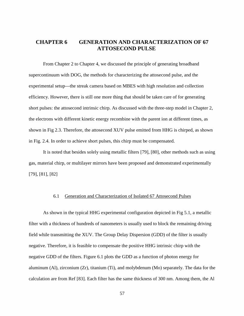
CHAPTER 6 GENERATION AND CHARACTERIZATION OF 67 ATTOSECOND PULSE
From Chapter 2 to Chapter 4, we discussed the principle of generating broadband
supercontinuum with DOG, the methods for characterizing the attosecond pulse, and the
experimental setup—the streak camera based on MBES with high resolution and collection
efficiency. However, there is still one more thing that should be taken care of for generating
short pulses: the attosecond intrinsic chirp. As discussed with the three-step model in Chapter 2,
the electrons with different kinetic energy recombine with the parent ion at different times, as
shown in Fig 2.3. Therefore, the attosecond XUV pulse emitted from HHG is chirped, as shown
in Fig. 2.4. In order to achieve short pulses, this chirp must be compensated.
It is noted that besides solely using metallic filters [79], [80], other methods such as using
gas, material chirp, or multilayer mirrors have been proposed and demonstrated experimentally
[79], [81], [82]
6.1 Generation and Characterization of Isolated 67 Attosecond Pulses
As shown in the typical HHG experimental configuration depicted in Fig 5.1, a metallic
filter with a thickness of hundreds of nanometers is usually used to block the remaining driving
field while transmitting the XUV. The Group Delay Dispersion (GDD) of the filter is usually
negative. Therefore, it is feasible to compensate the positive HHG intrinsic chirp with the
negative GDD of the filters. Figure 6.1 plots the GDD as a function of photon energy for
aluminum (Al), zirconium (Zr), titanium (Ti), and molybdenum (Mo) separately. The data for the
calculation are from Ref [83]. Each filter has the same thickness of 300 nm. Among them, the Al
57

filter can only transmit photon energies up to 70 eV, making it unsuitable for generating the
shortest attosecond pulses. However, it is the most robust filter of the group, so it is usually used
to test the system. The Zr filter has a relatively higher transmission from 60 to 200 eV which is
the spectral window where the HHG continuum usually covers. The GDD is also negative for
lower photon energies and gradually reach to zero around 130 eV. As a result, the Zr filter is a
good candidate for best compensation. Note that before 2012, the shortest single attosecond
pulses (with duration of 80 as) were generated using the AG technique with a 300 nm Zr filter.
The Ti filter is very similar to the Zr filter, but with lower transmission. The Mo filter transmits
the XUV photon energy above 75 eV. So it is suitable to be used for compensating a
supercontinuum generated at a higher energy band.
58

Figure 6.1 The transmission (black solid line) and material GDD (blue dash-dotted line) of (a) aluminum (b) zirconium (c) titanium, and (d) molybdenum.
Using metallic filters, the attochirp can be well compensated at lower energy which
seems to lead to a low cutoff. However, higher peak intensity inside the gate of DOG is still
needed for smaller attochirp. Therefore, an independent method for adjusting the spectral cutoff
of the HHG is needed under the condition of high peak intensity.
It is known that in high-order harmonic generation, the observable spectral cutoff is not
only determined by the response of individual atoms, but also by the coherent build-up of the
XUV photons along the generating media. As a result, the true experimental cutoff under
realistic conditions is usually smaller than the theoretically calculated value for a single atom.
59

The macroscopic cutoff can be expressed as 𝐼𝐼𝑝𝑝 + 𝛼𝛼𝑈𝑈𝑝𝑝, with α smaller than 3.17
depending on experimental phase-matching conditions [84]–[86]. Therefore, intentional phase
mismatch can be used to reduce the spectral region where the attochirp is not well compensated.
Experimentally this is achieved by simply adjusting the gas pressure inside the gas media
interacting with the driving laser.
A 7 fs IR laser with about 900 𝜇𝜇𝜇𝜇 pulse energy after the beam splitter (seen in Fig. 5.1) is
used as the driving field with the Double Optical Gating technique. The beam size after the beam
splitter is about 10 mm. An aperture with tunable diameter is used to limit the beam size for the
highest count rate. This phenomena has been observed by many researchers [87]–[90]: the
highest harmonic yield is reached with the balance of focal geometry and ionization (which
favors smaller apertures) and the harmonic dipole amplitude and phase (which favors large
apertures) [91]. In our experiments, a telescope is used to focus the beam, and it has been
noticed there is considerable astigmatism at the focal point which can be eliminated by limiting
the beam size after the aperture. Of course, a smaller beam size also leads to a lower peak
intensity, so there is a trade-off. Experimentally, the optimal aperture size is determined on a
daily basis to obtain a high cutoff as well as a reasonable count rate. Usually 500 𝜇𝜇𝜇𝜇 energy can
be used after the pinhole for attosecond pulse generation, and the peak intensity inside the gate is
estimated to be 1 × 10¹⁵𝑊𝑊/𝑐𝑐𝜇𝜇2.
60

Figure 6.2 XUV photoelectron spectrum generated by DOG in Ne gas with six different pressures. The length of the gas cell is 1 mm. The peak intensity at the center of the polarization gate is about 1 × 10¹⁵𝑊𝑊/𝑐𝑐𝜇𝜇2. (Reproduced from Zhao, Zhang, Chini, Wu, Wang & Chang, “Tailoring a 67 attosecond pulse through advantageous phase-mismatch. Optics Letters”, 37(18), 3891, 2012)
Under this condition, the photoelectron spectra with different gas pressure were recorded
by the MBES, as shown in Fig. 6.2. The Neon gas was used as the generating media, as
discussed in Chapter 3. It can be seen that when the neon backing pressure in the gas cell was
tuned from 0.03 to 0.33 bar, the cutoff photon energy was observed to decrease from 160 to 120
eV, corresponding to 𝐼𝐼𝑝𝑝 + 2.6𝑈𝑈𝑝𝑝 to 𝐼𝐼𝑝𝑝 + 1.8𝑈𝑈𝑝𝑝. If a proper backing pressure was chosen, the
HHG spectrum covered the bandwidth which can be best compensated.
As shown in Fig. 5.3, the GDD of a 300 nm Zr filter (pink dashed line) and the attochirp
(blue solid line) calculated with a peak intensity of 1 × 10¹⁵𝑊𝑊/𝑐𝑐𝜇𝜇2 are plotted. It can be seen
61

that the GDD of the filter is negative below 130 eV, which can compensate the positive
attochirp. In contrast, at an energy higher than 130 eV, the chirp is not well compensated.
Therefore, the spectrum (red solid line) should be chosen to match the area where the attochirp is
best compensated for generating the shortest attosecond pulses.
Figure 6.3 Attosecond intrinsic chirp compensated by a 300 nm Zr filter. The spectrum is specially chosen to cover the area where the attochirp is best compensated. Black solid line: XUV spectrum taken with 300 nm Zr filter. Red dashed line: intrinsic chirp of the attosecond pulses. Blue dash-dotted line: GDD of 300 nm Zr filter.
From Fig. 6.2, it can be seen that the backing pressure of 0.2 bar should be used in the
streaking experiment for the best match with the spectral range where the Zr filter can best
compensate the attochirp. An attosecond streaking experiment was done under this condition to
characterize the pulse duration. The streaking trace was shown in Fig. 6.4 (a), and retrieved
spectrum and temporal phase are shown in Fig. 5.6 (c) and (d) respectively. The CRAB and
62

PROOF methods were both applied to the experimental data and the same result of a single 67 as
pulse was obtained. In Fig. 5.6 (b), the filtered streaking trace with one omega frequency
𝐼𝐼𝜔𝜔𝐿𝐿(𝐼𝐼, 𝜏𝜏) (left) was compared with the retrieved one (right). The good agreement between those
two indicates the validity of the retrieval.
Figure 6.4 Characterization of a 67 as XUV pulse. (a) Streaked photoelectron spectrogram obtained experimentally. (b) Filtered 𝐼𝐼𝜔𝜔𝐿𝐿(𝐼𝐼, 𝜏𝜏) trace (left) from the spectrogram in (a) and the retrieved 𝐼𝐼𝜔𝜔𝐿𝐿(𝐼𝐼, 𝜏𝜏) trace (right). (c) Photoelectron spectrum obtained experimentally (thick grey solid) and retrieved spectra and spectral phases from PROOF (blue solid) and FROG-CRAB (red dashed). (d) Retrieved temporal profiles and phases from PROOF (blue solid) and FROG-CRAB (red dashed). (Reproduced from Zhao, Zhang, Chini, Wu, Wang & Chang, Tailoring a 67 attosecond pulse through advantageous phase-mismatch. Optics Letters, 37(18), 3891, 2012)
63

CHAPTER 7 ROUTE TO ATTOSEOCND PULSES WITH ONE ATOMIC UNIT OF TIME
With the Double Optical Gating technique, we have successfully demonstrated a single
isolated 67 as pulse. However, to reach even shorter pulse durations like 25 as, or one atomic
unit time, there are significant technical challenges.
First of all, for a transform-limited Gaussian pulse, 25 as in the time domain corresponds to a
75 eV FWHM in the spectral domain, which means that a total bandwidth of about 150 eV is
required. As discussed in Chapter 6, a Zr filter cannot be used for even shorter pulses since the
attochirp cannot be well compensated at energies above 130 eV. In addition, it filters out low
energy photons. Therefore, in order to reach 150 eV bandwidth, the photon spectrum needs to
extend to over 200 eV. This means higher peak intensities of the driving laser should be used and
a better filter for phase compensation needs to be implemented. It is noted that the attochirp is
inversely proportional to the intensity. Therefore, increasing intensity will benefit our goal in
both ways.
Secondly, the resolution for accurately retrieving a 25 as pulse is not easy to experimentally
achieve for such a high energy range. Simulations have been done to quantitatively determine the
necessary resolution for retrieving the contrast of isolated attosecond pulse with 1% accuracy. A
new type of MBES has been proposed to meet this requirement, and preliminary results were
obtained.
Finally, a new scheme for suppressing the driving field while transmitting the XUV has been
proposed to replace the metallic filters. This new scheme allows the transmission of photons
64

within the entire XUV spectral range, unlike the metal filters where only part of the photons can
be utilized. This new scheme is very useful to generate a super-broadband continuum spectrum.
In this chapter, we present the preliminary results regarding the route to achieving pulses
with a temporal duration of one atomic unit, discussing the three aspects mentioned above.
7.1 Broadband Supercontinuum Generation with Lens Focusing
In order to generate an even broader-bandwidth attosecond continuum, higher intensity is
needed inside the gate. The easiest way is to use a tighter focusing configuration for the input
driving laser. However, due to space limitations, further shortening the focal length using the two-
mirror configuration would introduce significant astigmatism. To reduce the astigmatism, a lens
can be used. However, it is commonly accepted that using lenses in ultrafast optics field leads to a
distortion of wavefront and a broadening effect of the pulse duration at the focus, due to the
material dispersion. However, it has been recently shown with calculation that pulses as short as 5
fs can be obtained at the focus as long as the input beam size and the focal length are properly
chosen [92].
Following the same procedure in Ref [92], we calculated the pulse duration near the focus
using the realistic parameters in our experiment. The input pulse is assumed to be a transform-
limited 7 fs Gaussian pulse and a 140 mm focal length was chosen. The beam size of the input
beam is assumed to be 6 mm in diameter, which is roughly the same as the current case after the
aperture. Therefore, the same pulse energy of around 500 𝜇𝜇𝜇𝜇 should be expected for the lens
focusing. As shown in Fig. 7.1, both the pulse duration and the spectrum at the focus are nearly
identical to the input beam. The lens here works like a slab with the same thickness to the driving
65

pulse. Therefore, a lens can be used in generating supercontinuum spectra and single attosecond
pulses.
Figure 7.1 Performance of the lens focusing a 7 fs TL input pulse, with a 3 mm beam waist on the lens surface. (a) The electric field in the temporal domain. Red solid line: input field. Blue dashed line: electric field at the focus. (b) The laser spectra. Red solid line: input field. Blue dashed line: electric field at the focus.
The new experimental configuration with the lens focusing is plotted in Fig. 7.2. The
gold-coated flat mirror after the toroidal mirror was removed to increase the photon flux for
66

generating photoelectrons. Under this condition, a photoelectron spectrum was taken by our TOF
spectrometer with a Mo filter, as shown in Fig. 5.8. The cutoff extended to 180 eV photon
energy, supporting 40 as pulses. The reason why the Mo filter was used here is that Mo filter
provides better phase compensation at higher photon energies.
Figure 7.2 A schematic drawing of the experimental configuration with the lens focusing configuration. BS: Beam Splitter; QP: Quartz Plate; M: Silver Mirror; L: lens with 140 mm focal length; GC: Gas Cell; MF: Metallic Filter; TM: Toroidal Mirror; HM: Hole drilled Mirror; MBES: Magnetic Bottle Electron Energy Spectrometer.
67

Figure 7.3 The supercontinuum spectrum measured with a 140 mm focal lens and a 300 nm molybdenum filter. The cutoff has extended to 180 eV photon energy. (b) The Fourier-transformed temporal spectrum assuming a TL pulse duration for the spectrum in (a). The FWHM is 40 as.
7.2 Characterizing the Contrast of 25 Attosecond Isolated Pulses
Isolated attosecond pulses can be used in pump-probe experiments to study fast electron
dynamics. This requires that the system cannot be disturbed besides the pump or probe beam.
68

However, for attosecond generation from HHG, it is always the case that certain satellite pulses
are generated along the main pulse, regardless of which gating technique is adopted. Therefore, it
is important to know the relative intensity of those satellite pulses. Typically the intensity of
those satellite pulses should be less than 10% of the main pulse to avoid disturbing the system
under investigation by the attosecond pump-attosecond probe experiments. To accurately
characterize the contrast of the attosecond pulse, there is one key factor for consideration, which
is the experimental spectral resolution, especially for 25 as pulses due to the ultra-broad spectral
range.
We simulated a 25 as transform-limited (TL) Gaussian pulse, with central energy at 150
eV, having pre- and post-pulses with 1% intensity contrast to the main pulse. The satellite pulses
are set to be 50 as in duration since the satellite pulses are usually generated with lower
intensities. With the DOG technique, the satellite pulse should be one full optical cycle away
from the main pulse, since the second harmonic break the symmetry of the driving laser. The
central wavelength of the driving laser is assumed to be 750 nm, which is the case for
Ti:Sapphire lasers. Therefore, the satellite pulses are 2,500 as away from the main pulse, as
depicted in Fig. 7.4 (a) (blue solid line). The Fourier-transform spectrum is shown in Fig. 7.4 (b)
(blue solid line), which extends from 30 eV to 220 eV. However, the spectrum can only be
measured experimentally with limited resolution. As a result, the final measurement should be
the convolution of the real spectrum and the MBES resolution, as discussed in Chapter 5.3. Since
the resolution depends on the spectral energy, the convolution is done by multiplying each
element in the spectrum by its corresponding response function and then adding them together.
Each response function has to be normalized to its area before the multiplication to ensure the
equal weight for all energies.
69

The red dashed line in Fig. 7.4 (b) represents the spectrum after the convolution.
Obviously it can been seen that the interference depth is reduced due to the limited instrumental
resolution.
To retrieve the satellite pulse contrast in the temporal domain, it is not sufficient to
perform a Fourier transform. Instead, a streaking spectrogram is generated with the XUV pulse
and a 5 fs, 750 nm near-infrared (NIR) streaking pulse which has a peak intensity of 5 ×
1011𝑊𝑊/𝑐𝑐𝜇𝜇2. The spectrum at each delay in the streaking spectrogram is independently
convoluted with the response function. Then the spectrum phase is characterized by the FROG-
CRAB technique, and the retrieved temporal intensity profile is plotted in Fig. 7.3 (a) (red
dashed line), as a comparison with the input pulse. It can be seen that the satellite pulse contrast
retrieved from the convoluted spectrum is only 0.16%, much smaller than the 1% true value. The
reason is the interference pattern between the satellite pulses and the main pulse is greatly
smeared out by the response function. Therefore, retrieval from the recorded spectrum
significantly underestimate the satellite pules contrast. (Best seen from the inset of Fig. 7.4 (b)).
70

Figure 7.4 Effects of the response function on characterizing satellite pulses (1% satellite pulse is assumed). (a) The blue solid line shows the input temporal pulse. The red dashed line with dot is the retrieved temporal pulse from the streaking trace. (b) The blue solid line shows the spectrum of the input pulse, and the red dashed line is the convoluted spectrum in a 3 m TOF. Inset shows the enlarged spectra from 120 to 140 eV.
Our simulation indicates that for 25 as pulses, better spectral resolution is desired for the
accurate characterization of the satellite pulses. To improve the spectrometer resolution, one
commonly increases the length of the flight tube of MBES. As explained in Chapter 5.2, the
photoelectrons with larger emission angles takes longer time to reach the MCP for detection.
This deviation ∆𝑡𝑡 are contributed from two parts: ∆𝑡𝑡1, the term before the parallelization
71

(roughly from 0 to 100 mm from the photoelectron birthplace), and ∆𝑡𝑡2, the term after the
parallelization (farther than 100 mm away). Increasing the length of the flight tube actually
increases ∆𝑡𝑡2 proportional to the total flight time 𝐸𝐸, while keep the ∆𝑡𝑡1unchanged. As a result,
the overall ratio which determines the spectral resolution ∆𝑡𝑡 𝐸𝐸� is smaller, hence improving the
resolution. A comparison of the spectral deviation and response function (in other words, the
instrumental resolution) at 150 eV for three-meter and eight-meter flight tubes are shown in Fig.
7.5. It can be seen that the eight-meter MBES clearly measures the electron kinetic energy more
accurately, and the response function is narrower. Further simulation with the streaking trace
retrieval shows that with an eight-meter-long flight tube, the retrieved 1% satellite pulse is
0.36%. Even though the satellite pulse is retrieved more accurately than with the three-meter
flight tube, it is still three times smaller than the real value.
72

Figure 7.5(a) Ratio of the energy calculated from the flight time (ETOF) to the real value (Ei) as a function of the emission angle. Electrons with emission angles larger than 107° cannot be detected by the MCP. (b) Energy distribution of 180 eV monoenergetic electrons calculated assuming the angular distribution of Ne photoionization with an asymmetric parameter of 1.4, which is referred to as the response function. The solid line is for a spectrometer with 3 m flight distance; and the dashed line is for an 8 m TOF. (Reprinted from Q Zhang, K. Zhao, and Z. Chang, “High resolution electron spectrometers for characterizing the contrast of isolated 25 as pulses”. Journal of Electron Spectroscopy and Related Phenomena, 195, pp 48-54. DOI: 10.1016/j.elspec.2014.05.008 )
Further increasing the flight tube could not significantly improve the energy resolution
because the error introduced during the increased flight distance starts to play a role. This
means ∆𝑡𝑡2 ≫ ∆𝑡𝑡1, therefore, ∆𝑡𝑡𝑇𝑇≈ ∆𝑡𝑡2
𝑇𝑇. In this scenario, increasing the length of the flight tube
73

increases the ∆𝑡𝑡2 and 𝐸𝐸. However, their ratio ∆𝑡𝑡𝑇𝑇
and hence the spectral resolution stays
unchanged.
Alternately, the response function of the TOF can be further improved by eliminating
electrons with large emission angles. Actually, in the attosecond streaking experiment, electrons
emitted with large angles are highly unwanted because the streaking effects decrease with
emission angle. Electrons emitted with angles larger than 90° will be streaked in the opposite
direction. Therefore it would be ideal to block the large angle electrons for both the benefit of the
streaking data quality and energy resolution. Given the fact that electrons with larger emission
angle deviate transversely away from the axis of the flight tube more as they fly in the magnetic
field, a pinhole can effectively block those electrons. Theoretically the pinhole can be put
anywhere between the generation point of the photoelectrons and the electron detector. However,
experimentally it is much easier to put it at the beginning of the electron trajectory. We plotted
the relation between the pinhole size and the collection angle as shown in Fig. 7.6 (a) and (b).
The pinhole size varies from 0.15 to 0.4 mm and is placed 2 mm away from the electron
birthplace. Then the new response function with different pinhole size can be calculated from the
revised collection angle. Particularly, the response functions of 180 eV electrons for a 0.25 mm
pinhole in an eight-meter TOF, are shown in Fig. 7.7. Comparing with the response function
without the pinhole (red dashed line in Fig. 7.7), it can be seen that the long tail of the response
function is eliminated, and the FWHM is 0.19 eV for the eight-meter TOF.
To study the effects of the pinhole size on the accuracy of satellite pulse contrast
measurements, we simulated the streaking trace using the spectra convoluted with the new
response functions and plotted the retrieved satellite pulse contrast as a function of pinhole size
74

in Fig. 7.8. To compare, the real value is also plotted for satellite pulses with intensities of 1% of
the main pulses. This figure shows that as pinhole size decreases, the satellite pulse
characterization becomes more accurate, as expected. Particularly, a 0.25 mm pinhole in an
eight-meter TOF can be chosen to retrieve the satellite pulse ratio with less than 10% error. On
the other hand, the collection efficiency is also reduced to 15%.
Figure 7.6 (a) Collection angle and (b) collection efficiency as functions of the electron energy for different pinhole diameters.
75

Figure 7.7 Response function calculated with a 0.25 mm pinhole in the 8 m TOF, for 180 eV electrons (blue solid line). The response function without is plotted with red dashed line for comparison.
76
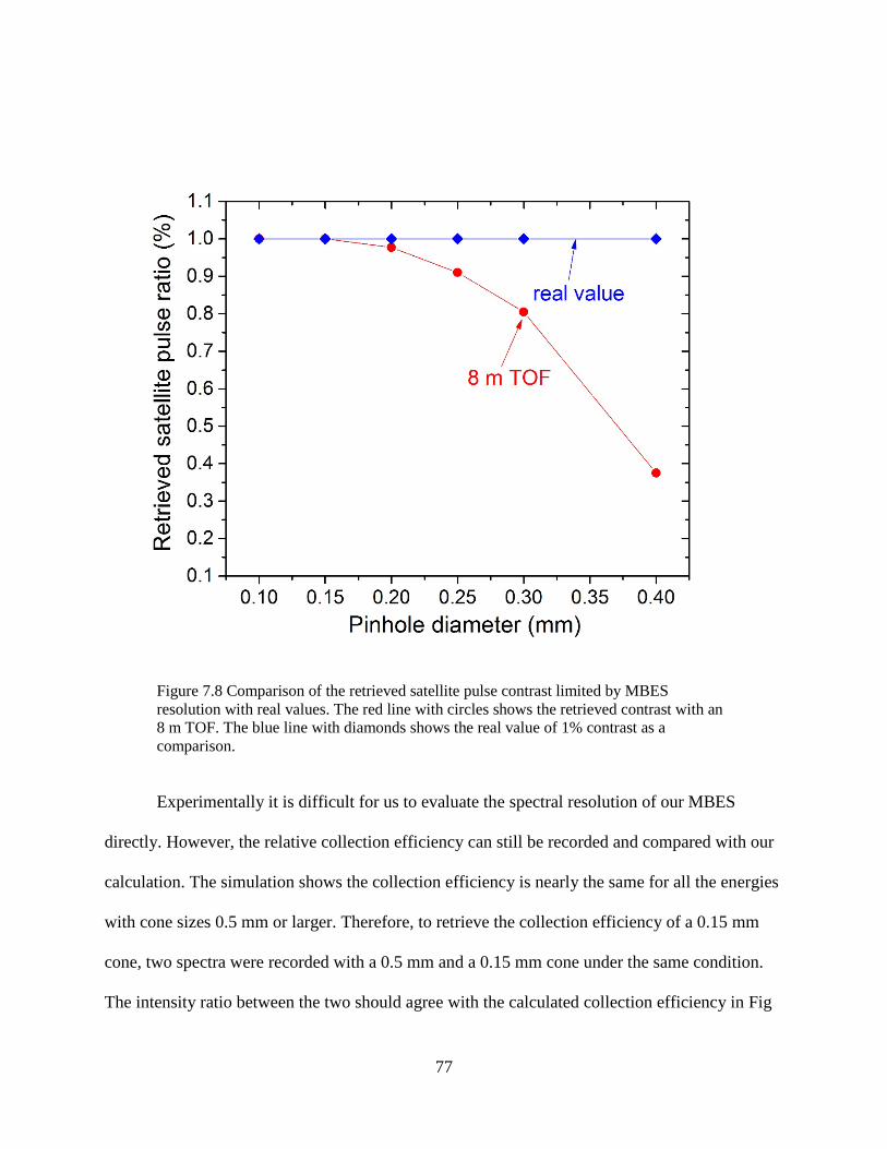
Figure 7.8 Comparison of the retrieved satellite pulse contrast limited by MBES resolution with real values. The red line with circles shows the retrieved contrast with an 8 m TOF. The blue line with diamonds shows the real value of 1% contrast as a comparison.
Experimentally it is difficult for us to evaluate the spectral resolution of our MBES
directly. However, the relative collection efficiency can still be recorded and compared with our
calculation. The simulation shows the collection efficiency is nearly the same for all the energies
with cone sizes 0.5 mm or larger. Therefore, to retrieve the collection efficiency of a 0.15 mm
cone, two spectra were recorded with a 0.5 mm and a 0.15 mm cone under the same condition.
The intensity ratio between the two should agree with the calculated collection efficiency in Fig
77

7.6. As it can be seen in Fig. 7.9 (b), the agreement between the experiment and the calculation
are reasonable. The difference between the two might be due to the fact that the photoelectrons
are born in a line along the XUV propagation rather than a single spot. The offset of the electron
starting position further complicates the problem and is difficult to simulate. Further
experimental tests are still needed to best understand this process.
Figure 7.9 Experimental evaluation of the collection efficiency of the 0.15 mm and 0.5 mm cone. (a) The spectra taken with 0.15 mm (black solid) and 0.5 mm (red solid) cone size under the same condition. The 200 nm thick Be filter was used to block the IR and
78

select the energy range between 0~90eV. (b) The collection efficiency dependence on the electron energy for 0.15 mm. The black line shows the experimental result calculated from (a) and the red line shows the calculation from Fig 7.6.
79

7.3 Suppressing the Driving Laser with Microchannel Plate
As was discussed in previous chapters, the metallic filters were used to block the
remaining driving field while transmitting the XUV photons. Since the conversion efficiency of
the HHG is usually on the order of 10-4~10-5, the driving pulse energy is practically unchanged
after HHG. Separating the driving pulse from the high-order harmonics is a long-standing
problem for the attosecond community.
There have been several other proposals dealing with this issue besides inserting metallic
filters. Using conical-shaped driving lasers, specially-designed beam splitters, Si/SiC plates at
Brewster’s angle, and XUV grating pairs can all successfully separate the IR and the XUV [93]–
[96]. However, each one of those schemes has certain shortcomings.
As shown in Fig. 7.10 (a), a metallic filter is usually directly placed after the HHG gas
cell to block the driving pulse (red) and transmit the generated XUV (blue). However, metallic
filters only transmit the XUV photon within certain energy windows. For example, an Al filter
only transmits XUV photons up to 72 eV. A Zr filter cannot transmit the XUV below 60 eV.
Using this method, a significant portion of the supercontinuum bandwidth is lost. Moreover, the
metallic filters are extremely fragile and easy to break. They are not suitable for blocking driving
lasers with a pulse energy of 100 mJ or above.
Using an annular driving beam can perfectly separate the remaining driving laser without
the issues posed by metallic filters. It is achieved by blocking the center portion of the incoming
beam, and only the outside part is used to generate attosecond pulse, as shown in Fig. 7.10 (b).
Obviously this is a huge waste, especially when higher pulse energy is employed in HHG.
80

It has also been proposed that using specially-designed multilayer beam splitters can
solve this issue. However, this method only works for XUV photons below 75 eV. The same
limitation applies to using Si/SiC plate at Brewster angle. A grating pair can be used for any
photon energy. However, it only works with narrow band spectral range due to the spatial and
temporal dispersion introduced. Schematic drawings for those two methods are shown in Fig.
7.10 (c) and (d) separately.
81
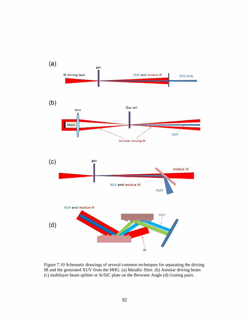
Figure 7.10 Schematic drawings of several common techniques for separating the driving IR and the generated XUV from the HHG. (a) Metallic filter. (b) Annular driving beam (c) multilayer beam splitter or Si/SiC plate on the Brewster Angle (d) Grating pairs.
82

Here, we propose a new scheme: using a Microchannel Plate as a short-pass filter to
suppress the driving infrared laser relative to the XUV photons without any spectral limitation.
Essentially an MCP consists of millions of parallel glass capillaries (microscopic channels)
leading from one surface to the other [97]. The diameter of each channel inside the MCP is
several micrometers, comparable to the wavelength of NIR/MIR but much larger than that of the
XUV or soft x-ray photons. As a result, the driving laser experiences a significant diffraction
effect after the MCP, while the XUV remains largely unchanged, meaning the transmission of
the driving field should be significantly smaller than that of the XUV photons after the MCP.
Therefore, the driving pulse is relatively suppressed. A schematic drawing of the principle of the
MCP is shown in Fig. 7.11.
In order to demonstrate this new technique, the zero-order transmission of the MCP was
measured as a function of wavelength. Three lasers with different wavelengths are available for
testing the MCP transmission. The home-built Ti:Sapphire laser has a central wavelength of 750
nm and pulse duration of 23 fs. The MIR output from a commercial TOPAS has a central
wavelength of 1.6 µm and pulse duration of 50 fs. A continuous-wave laser with a wavelength at
532 nm is also used. The measured zero-order transmission with these three different
wavelengths are plotted in Fig. 7.10, varying from the lowest transmission of 0.4% for 1.6 µm to
11% for 532 nm wavelength. For the Ti:Sapphire laser, which is used for HHG in our current
setup, the transmission is about 5%. Obviously the transmission is much larger for shorter
wavelengths.
To separate the XUV and the driving pulse effectively, the transmission of the two
through the MCP must be largely different. The total MCP transmission in the XUV spectral
region has been measured to be as high as 60% for photon energies from 50 eV to 1.5 keV [98],
83

reaching the upper limit set by the MCP opening ratio. For photons with even higher energy, the
transmission should be the same due to their shorter wavelength. In our scenario, only the zero
order transmission should be used for studying ultrafast dynamics, and therefore the transmission
should be evaluated carefully. Experimentally, we placed the filter in the same position as the
metallic filter in our HHG beam line. Higher orders of the diffracted light were blocked by a hole
mirror, and eventually only the zero-order transmission contributes to the photoelectron spectrum
recorded by the MBES. The measured transmission was also plotted in Fig.7.12.
Figure 7.11 Schematic drawing of the principle of the MCP filter. The diameter of each MCP channel is comparable to the wavelength of the IR but much larger than that of the XUV. The red (blue) lines indicate the IR (XUV) beam. The 0th, ±1st order diffractions are labeled by black arrows. (Reprinted from Q Zhang, K. Zhao, J. Li, M. Chini, Y. Cheng, Y. Wu, E. Cunningham, and Z. Chang, “Suppression of Driving Laser in High Harmonic Generation with a Microchannel Plate”. Opt. Lett. Vol. 39, Issue 12, pp. 3670-3673 (2014), http://dx.doi.org/10.1364/OL.39.003670)
84

Figure 7.12 The zero-order transmission of the MCP for (a) XUV photons and (b) visible or longer wavelengths. The red line in (a) is the transmission measured with a 300 nm Zr filter and a 300 nm Al filter.
Since only the zero-order of the transmission is used for the attosecond applications, one
would not expect any degradation of the spatial or temporal properties of the XUV pulses. To
confirm this judgment, a RABITT (Reconstruction of Attosecond Beating By Interference of
Two-photon Transitions) scan with an attosecond pulse train was done with and without the
MCP filter, as shown in Fig. 7.13 (a) below [42], [99]. Similar to the attosecond streaking, a
RABBITT measurement involves an attosecond pulse train and a weak IR beam that are
temporally and spatially overlapped, and the photoelectrons generated by the attosecond pulse
train can absorb or emit one IR photon energy. Experimentally this means a sideband can be
observed in addition to discrete harmonic from the attosecond pulse train. The relative temporal
85

(delay) position of the sideband maximum on a RABITT spectrogram is determined by the phase
difference between the two adjacent odd harmonic orders. More details about RABITT can be
found in Chapter 4.1. The delay-dependent signal of the sideband contains the spectral phase
information, allowing for the characterization of the attosecond pulses. The black dashed lines in
Fig. 7.13 (a) represent the temporal variation for each harmonic order. The slopes determine the
group delay of the attosecond pulse train. As can be seen in Fig. 7.13 (b), the group delay are
identical for the attosecond pulse trains obtained with and without an MCP filter. This
experimental result conclusively demonstrated the dispersion of the attosecond pulse is not
affected by the MCP filter. This is a key conclusion for the attosecond community.
The damage threshold is another key factor for the MCP filter to be practically used. In
our case, it is difficult to define when the filter is damaged. For example: for a 1 kHz, 750 nm
Ti:Sapphire laser, the surface of the MCP shows dark spot several minutes after the incident of
laser with peak intensity of 0.2 TW/cm2. However, the transmission efficiency for the 750 nm
laser remained the same even after the surface darkened. This is probably due to the fact that the
transmission of the MCP filter only depends on the structure of the multichannel inside the MCP,
while the dark spots indicates the surface coating or substrates are damaged. Nevertheless, it is
safe to the say that the damage threshold should be at least 0.2 TW/cm2 for a 1 kHz Ti:Sapphire
pump laser. For the same laser but with a 10 Hz repetition rate, the dark spot only shows when
the peak intensity reaches 0.6 TW/cm2. This value is similar to the damage threshold using a
Si/SiC plate at Brewster’s angle. The latter has been practically used in terawatt-level 10 Hz
Ti:Sapphire laser systems for high-flux isolated attosecond pulse generation [100].
86
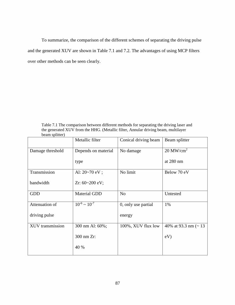
To summarize, the comparison of the different schemes of separating the driving pulse
and the generated XUV are shown in Table 7.1 and 7.2. The advantages of using MCP filters
over other methods can be seen clearly.
Table 7.1 The comparison between different methods for separating the driving laser and the generated XUV from the HHG. (Metallic filter, Annular driving beam, multilayer beam splitter)
Metallic filter Conical driving beam Beam splitter
Damage threshold Depends on material
type
No damage 20 MW/cm2
at 280 nm
Transmission
bandwidth
Al: 20~70 eV ;
Zr: 60~200 eV;
No limit Below 70 eV
GDD Material GDD No Untested
Attenuation of
driving pulse
10-6 ~ 10-7 0, only use partial
energy
1%
XUV transmission 300 nm Al: 60%;
300 nm Zr:
40 %
100%, XUV flux low 40% at 93.3 nm (~ 13
eV)
87

Table 7.2 The comparison between different methods for separating the driving laser and the generated XUV from the HHG. (Si/SiC plate, Grating pairs, MCP filter)
Si/SiC plate at
Brewster Angle
Grating pair MCP filter
Damage threshold 0.8 TW/cm2
(10 Hz, 800 nm laser)
Grazing incident
angle
0.6 TW/cm2 (10 Hz,
750 nm laser)
Transmission
bandwidth
Below 120 eV No limit. Narrow
bandwidth
No limit
GDD No High due to grating No
Attenuation of
driving pulse
~ 10-4 0 5% for 750 nm, 0.4%
for 1.6 𝜇𝜇𝜇𝜇
XUV transmission ~ 60% at 29.6 nm (~
42 eV)
20% Higher than 25 %
88

Figure 7.13(a) RABBITT spectrograms with (left) and without (right) MCP filter. (b) The relative delay for sideband maxima as the function of the photoelectron energy. The red squares were taken with Al and MCP filter, and the blue dots were taken with Al filter only. The linear fits for each dataset were plotted in the solid and dashed lines with the same color. (Reprinted from Q Zhang, K. Zhao, J. Li, M. Chini, Y. Cheng, Y. Wu, E. Cunningham, and Z. Chang, “Suppression of Driving Laser in High Harmonic Generation with a Microchannel Plate”. Opt. Lett. Vol. 39, Issue 12, pp. 3670-3673 (2014), http://dx.doi.org/10.1364/OL.39.003670)
89

CHAPTER 8 CONCLUSIONS AND OUTLOOK
In this thesis, I have presented the generation and characterization of a single isolated 67
as pulse, which is the shortest optical pulse so far. The DOG method was employed to generate a
super-broadband continuum spectrum from HHG. The PROOF method was used for ultra-short
attosecond pulse characterization. Experimentally, an electron energy spectrometer with high
resolution and collection efficiency is built for attosecond streaking experiments. Finally, several
important issues regarding a single 25 as pulse have been discussed. The intensity can be
improved by using a tight-focus lens, and the bandwidth of the HHG can increase by using a
MCP filter to suppressing the remaining driving filed. The resolution of the MBES can be greatly
enhanced by placing a pinhole near the entrance of the MBES, leading to the retrieval of the
contrast of satellite pulses around the isolated attosecond pulse with 90% accuracy.
For future work, a driving laser centered at longer wavelengths, i.e. a few-cycle mid-
infrared femtosecond laser, should be used. As shown in equation 2.9, the cutoff the HHG is
proportional to not only peak intensity, but also to the square of the wavelength of the driving
laser when the laser intensity is below the saturation intensity [101], [102]. Consequently, at the
same intensity level as the current scenario, a cutoff over 200 eV can be easily achieved. More
importantly, the attochirp is also inversely proportional to the wavelength. Therefore, using the
driving lasers with longer wavelength benefits our goal in both ways.
90

APPENDIX A: LIST OF PUBLICATIONS
91

Peer-Reviewed Journal Publications
Q. Zhang, K. Zhao, and Z. Chang, “Determining Time Resolution of Microchannel Plate
Detectors for Electron Time-of-Flight Spectrometer”, Review of Scientific Instruments 81, 073112, 2010
X. Wang, M. Chini, Q. Zhang, K. Zhao, Y. Wu, Dmitry A. Telnov, Shih-I Chu, and Z. Chang,
“Mechanism of quasi-phase-matching in a dual-gas multijet array”, Physical Review A, 86, pp. 021802, 2012
K. Zhao, Q. Zhang, M. Chini, Y. Wu, X. Wang, and Z. Chang, “Tailoring a 67 attosecond pulse
through advantageous phase-mismatch”, Optics Letters 37(18), pp.3891-3893, 2012 Q. Zhang, K. Zhao, J. Li, M. Chini, Y. Cheng, Y. Wu, E. Cunningham, and Z. Chang,
“Suppression of Driving Laser in High Harmonic Generation with a Microchannel Plate”, Optics Letters (Accepted)
Q. Zhang, K.Zhao, and Z. Chang, “High resolution electron spectrometers for characterizing the
contrast of isolated 25 as pulses”, Journal of Electron Spectroscopy and Related Phenomena (Accepted)
92

Invited Book Chapters
K. Zhao, Q. Zhang, M. Chini & Z. Chang, “Route to One Atomic Unit of Time – Development of a Broadband Attosecond Streak Camera”, in Multiphoton Processes and Attosecond Physics Vol. 125 (eds. K. Yamanouchi & K. Midorikawa), Ch. 19, pg. 109 (Springer, 2012).
Q. Zhang, K. Zhao, M. Chini. Y. Wu and Z. Chang, “Ultrabroadband Coherent Light for
Shortest Attosecond Laser Pulse”, in The Supercontinuum Laser Source (3rd edition) (to be published)
93

Conference Presentations
Q. Zhang, K. Zhao, M. Chini, Y. Wu, X. Wang, and Z. Chang, “Generation and characterization of broadband isolated attosecond pulse”, American Physical Society, 43rd Annual Meeting of the APS Division of Atomic, Molecular and Optical Physics, June 4-8,2012. (Oral Presentation)
Kun Zhao, Qi Zhang, Michael Chini, Sabih D. Khan, Steve Gilbertson, and Zenghu Chang,
Isolated 80 as XUV pulses characterized by PROOF, American Physical Society Division of Atomic, Molecular and Optical Physics Annual Meeting, June 13-17, 2011, Atlanta, GA
Q. Zhang, K. Zhao and Z. Chang, “Magnetic-bottle electron spectrometer for measuring 25 as
pulses”, American Physical Society, 41st Annual Meeting of the APS Division of Atomic, Molecular and Optical Physics Volume 55, Number 5, March 25-29, 2010 (Oral Presentation)
Kun Zhao, Michael Chini, Qi Zhang, Steve Gilbertson, Sabih D. Khan, and Zenghu Chang,
Isolated 80-Attosecond Pulses Characterized by PROOF, 2010 Attosecond MURI Review (Multidisciplinary University Research Initiative: Attosecond Optical Technology Based on Recollision and Gating), Dec 7, 2010, Orlando, FLChini, M., Wang, H., Mashiko, H., Chen, S., Yun, C., Gilbertson, S. & Chang, Z. Interferometric Delay Control in Attosecond Streaking Experiments. 2nd International Conference on Attosecond Physics, Manhattan KS (2009).
Patents Q. Zhang, K. Zhao and Z. Chang, “Microchannel Plate as an effective filter for suppressing
infrared light in High-order Harmonic beams”, US patent, (2014, pending)
94

APPENDIX B: COPYRIGHT PERMISSION
95

96
97

98

99

100

101

102

103

104

105

106

LIST OF REFERENCES
[1] T. H. MAIMAN, “Stimulated Optical Radiation in Ruby,” Nature, vol. 187, no. 4736, pp. 493–494, Aug. 1960.
[2] A. Schawlow and C. Townes, “Infrared and Optical Masers,” Phys. Rev., vol. 112, no. 6, pp. 1940–1949, Dec. 1958.
[3] A. E. Siegman, Lasers. University Science Books, 1986.
[4] Light and Its Uses. Scientific American, 1974, pp. 40 – 43.
[5] O. Albert, H. Wang, D. Liu, Z. Chang, and G. Mourou, “Generation of relativistic intensity pulses at a kilohertz repetition rate,” Opt. Lett., vol. 25, no. 15, p. 1125, Aug. 2000.
[6] K. Zhao, Q. Zhang, M. Chini, Y. Wu, X. Wang, and Z. Chang, “Tailoring a 67 attosecond pulse through advantageous phase-mismatch,” Opt. Lett., vol. 37, no. 18, p. 3891, Sep. 2012.
[7] E. Goulielmakis, M. Schultze, M. Hofstetter, V. S. Yakovlev, J. Gagnon, M. Uiberacker, A. L. Aquila, E. M. Gullikson, D. T. Attwood, R. Kienberger, F. Krausz, and U. Kleineberg, “Single-Cycle Nonlinear Optics,” Science (80-. )., vol. 320, p. 1614, 2008.
[8] P. Nuernberger, G. Vogt, T. Brixner, and G. Gerber, “Femtosecond quantum control of molecular dynamics in the condensed phase.,” Phys. Chem. Chem. Phys., vol. 9, no. 20, pp. 2470–97, May 2007.
[9] O. Gessner, A. M. D. Lee, J. P. Shaffer, H. Reisler, S. V Levchenko, A. I. Krylov, J. G. Underwood, H. Shi, A. L. L. East, D. M. Wardlaw, E. T. H. Chrysostom, C. C. Hayden, and A. Stolow, “Femtosecond multidimensional imaging of a molecular dissociation.,” Science, vol. 311, no. 5758, pp. 219–22, Jan. 2006.
[10] P. H. Bucksbaum, “Chemistry. The first femtosecond in the life of a chemical reaction.,” Science, vol. 312, no. 5772, pp. 373–4, Apr. 2006.
[11] F. Seifert, V. Petrov, and M. Woerner, “Solid-state laser system for the generation of midinfrared femtosecond pulses tunable from 3.3 to 10 microm.,” Opt. Lett., vol. 19, no. 23, pp. 2009–11, Dec. 1994.
[12] A. H. Zewail, “Laser femtochemistry.,” Science, vol. 242, no. 4886, pp. 1645–53, Dec. 1988.
107

[13] G. Krauss, S. Lohss, T. Hanke, A. Sell, S. Eggert, R. Huber, and A. Leitenstorfer, “Synthesis of a single cycle of light with compact erbium-doped fibre technology,” Nat. Photonics, vol. 4, no. 1, pp. 33–36, Dec. 2009.
[14] M. Yamashita, K. Yamane, and R. Morita, “Quasi-automatic phase-control technique for chirp compensation of pulses with over-one-octave bandwidth-generation of few- to mono-cycle optical pulses,” IEEE J. Sel. Top. Quantum Electron., vol. 12, no. 2, pp. 213–222, Mar. 2006.
[15] M. Hentschel, R. Kienberger, C. Spielmann, G. A. Reider, N. Milosevic, T. Brabec, P. Corkum, U. Heinzmann, M. Drescher, and F. Krausz, “Attosecond metrology.,” Nature, vol. 414, no. 6863, pp. 509–13, Nov. 2001.
[16] F. Frank, C. Arrell, T. Witting, W. a Okell, J. McKenna, J. S. Robinson, C. a Haworth, D. Austin, H. Teng, I. a Walmsley, J. P. Marangos, and J. W. G. Tisch, “Invited review article: technology for attosecond science.,” Rev. Sci. Instrum., vol. 83, no. 7, p. 071101, Jul. 2012.
[17] Z. Chang and P. Corkum, “Attosecond photon sources: the first decade and beyond [Invited],” J. Opt. Soc. Am. B, vol. 27, no. 11, p. B9, Oct. 2010.
[18] Z. Chang, Fundamentals of Attosecond Optics. Boca Raton, Florida: CRC Press, 2011.
[19] S. Nagele, R. Pazourek, J. Feist, K. Doblhoff-Dier, C. Lemell, K. Tőkési, and J. Burgdörfer, “Time-resolved photoemission by attosecond streaking: extraction of time information,” J. Phys. B At. Mol. Opt. Phys., vol. 44, no. 8, p. 081001, Apr. 2011.
[20] J. M. Dahlström, a L’Huillier, and a Maquet, “Introduction to attosecond delays in photoionization,” J. Phys. B At. Mol. Opt. Phys., vol. 45, no. 18, p. 183001, Sep. 2012.
[21] M. F. Kling and M. J. J. Vrakking, “Attosecond electron dynamics.,” Annu. Rev. Phys. Chem., vol. 59, no. November 2007, pp. 463–92, Jan. 2008.
[22] K. Klünder, J. M. Dahlström, M. Gisselbrecht, T. Fordell, M. Swoboda, D. Guénot, P. Johnsson, J. Caillat, J. Mauritsson, a. Maquet, R. Taïeb, and a. L’Huillier, “Probing Single-Photon Ionization on the Attosecond Time Scale,” Phys. Rev. Lett., vol. 106, no. 14, p. 143002, Apr. 2011.
[23] M. Schultze, M. Fiess, N. Karpowicz, J. Gagnon, M. Korbman, M. Hofstetter, S. Neppl, a L. Cavalieri, Y. Komninos, T. Mercouris, C. a Nicolaides, R. Pazourek, S. Nagele, J. Feist, J. Burgdörfer, a M. Azzeer, R. Ernstorfer, R. Kienberger, U. Kleineberg, E. Goulielmakis, F. Krausz, and V. S. Yakovlev, “Delay in photoemission.,” Science, vol. 328, no. 5986, pp. 1658–62, Jun. 2010.
108

[24] E. Goulielmakis, Z.-H. Loh, A. Wirth, R. Santra, N. Rohringer, V. S. Yakovlev, S. Zherebtsov, T. Pfeifer, A. M. Azzeer, M. F. Kling, S. R. Leone, and F. Krausz, “Real-time observation of valence electron motion.,” Nature, vol. 466, no. 7307, pp. 739–43, Aug. 2010.
[25] H. J. Wörner, J. B. Bertrand, D. V Kartashov, P. B. Corkum, and D. M. Villeneuve, “Following a chemical reaction using high-harmonic interferometry.,” Nature, vol. 466, no. 7306, pp. 604–7, Jul. 2010.
[26] a L. Cavalieri, N. Müller, T. Uphues, V. S. Yakovlev, a Baltuska, B. Horvath, B. Schmidt, L. Blümel, R. Holzwarth, S. Hendel, M. Drescher, U. Kleineberg, P. M. Echenique, R. Kienberger, F. Krausz, and U. Heinzmann, “Attosecond spectroscopy in condensed matter.,” Nature, vol. 449, no. 7165, pp. 1029–32, Oct. 2007.
[27] M. Ferray, A. L’Huillier, X. F. Li, L. A. Lompre, G. Mainfray, and C. Manus, “Multiple-harmonic conversion of 1064 nm radiation in rare gases,” J. Phys. B, vol. 21, p. 31, 1988.
[28] P. Maine, D. Strickland, P. Bado, M. Pessot, and G. Mourou, “Generation of ultrahigh peak power pulses by chirped pulse amplification,” IEEE J. Quantum Electron., vol. 24, no. 2, pp. 398–403, Feb. 1988.
[29] D. Strickland and G. Mourou, “Compression of amplified chirped optical pulses,” Opt. Commun., vol. 56, no. 3, pp. 219–221, Dec. 1985.
[30] G. Sansone, E. Benedetti, F. Calegari, C. Vozzi, L. Avaldi, R. Flammini, L. Poletto, P. Villoresi, C. Altucci, R. Velotta, S. Stagira, S. De Silvestri, and M. Nisoli, “Isolated single-cycle attosecond pulses.,” Science, vol. 314, no. 5798, pp. 443–6, Oct. 2006.
[31] H. Mashiko, S. Gilbertson, C. Li, S. D. Khan, M. M. Shakya, E. Moon, and Z. Chang, “Double Optical Gating of High-Order Harmonic Generation with Carrier-Envelope Phase Stabilized Lasers,” Phys. Rev. Lett., vol. 100, no. 10, p. 103906, Mar. 2008.
[32] Z. Chang, “Controlling attosecond pulse generation with a double optical gating,” Phys. Rev. A, vol. 76, p. 051403(R), 2007.
[33] S. Gilbertson, H. Mashiko, C. Li, S. D. Khan, M. M. Shakya, E. Moon, and Z. Chang, “A low-loss, robust setup for double optical gating of high harmonic generation,” Appl. Phys. Lett., vol. 92, p. 71109, 2008.
[34] H. Mashiko, S. Gilbertson, M. Chini, X. Feng, C. Yun, H. Wang, S. D. Khan, S. Chen, and Z. Chang, “Extreme ultraviolet supercontinua supporting pulse durations of less than one atomic unit of time,” vol. 34, no. 21, pp. 3337–3339, 2009.
109

[35] P. Corkum, “Plasma perspective on strong field multiphoton ionization,” Phys. Rev. Lett., vol. 71, no. 13, pp. 1994–1997, Sep. 1993.
[36] G. Mainfray and G. Manus, “Multiphoton ionization of atoms,” Reports Prog. Phys., vol. 54, no. 10, pp. 1333–1372, Oct. 1991.
[37] A. Scrinzi, M. Geissler, and T. Brabec, “Ionization Above the Coulomb Barrier,” Phys. Rev. Lett., vol. 83, no. 4, pp. 706–709, Jul. 1999.
[38] L. V. Keldysh, “Ionization in the filed of a strong elecromagnetic wave,” JETP, vol. 20, no. 5, p. 1307, 1964.
[39] M. Bellini, C. Lyngå, A. Tozzi, M. Gaarde, T. Hänsch, A. L’Huillier, and C.-G. Wahlström, “Temporal Coherence of Ultrashort High-Order Harmonic Pulses,” Phys. Rev. Lett., vol. 81, no. 2, pp. 297–300, Jul. 1998.
[40] M. Gaarde, F. Salin, E. Constant, P. Balcou, K. Schafer, K. Kulander, and a. L’Huillier, “Spatiotemporal separation of high harmonic radiation into two quantum path components,” Phys. Rev. A, vol. 59, no. 2, pp. 1367–1373, Feb. 1999.
[41] K. Varjú, P. Johnsson, T. Remetter, E. Gustafsson, E. Constant, E. Cormier, E. Mével, and A. L. Huillier, “Experimental Studies of Attosecond Pulse Trains,” vol. 15, no. 6, pp. 888–898, 2005.
[42] P. M. Paul, E. S. Toma, P. Breger, G. Mullot, F. Auge, P. Balcou, H. G. Muller, and P. Agostini, “Observation of a train of attosecond pulses from high harmonic generation.,” Science, vol. 292, no. 5522, pp. 1689–92, Jun. 2001.
[43] P. Antoine, A. L’Huillier, M. Lewenstein, P. Salières, and B. Carré, “Theory of high-order harmonic generation by an elliptically polarized laser field,” Phys. Rev. A, vol. 53, no. 3, pp. 1725–1745, Mar. 1996.
[44] K. Budil, P. Salières, M. Perry, and A. L’Huillier, “Influence of ellipticity on harmonic generation,” Phys. Rev. A, vol. 48, no. 5, pp. R3437–R3440, Nov. 1993.
[45] P. B. Corkum, N. H. Burnett, and M. Y. Ivanov, “Subfemtosecond pulses,” Opt. Lett., vol. 19, no. 22, p. 1870, Nov. 1994.
[46] R. Trebino, K. W. Delong, D. N. Fittinghoff, J. N. Sweetser, B. A. Richman, M. A. Krumbu, and D. J. Kane, “REVIEW ARTICLE Measuring ultrashort laser pulses in the time-frequency domain using frequency-resolved optical gating,” vol. 68, no. 9, pp. 3277–3295, 1997.
110

[47] K. W. DeLong, D. N. Fittinghoff, R. Trebino, B. Kohler, and K. Wilson, “Pulse retrieval in frequency-resolved optical gating based on the method of generalized projections,” Opt. Lett., vol. 19, no. 24, p. 2152, Dec. 1994.
[48] B. Shan, S. Ghimire, and Z. Chang, “Effect of orbital symmetry on high-order harmonic generation from molecules,” Phys. Rev. A, vol. 69, no. 2, p. 021404, Feb. 2004.
[49] C. Lyngå, A. L’Huillier, and C.-G. Wahlström, “High-order harmonic generation in molecular gases,” J. Phys. B At. Mol. Opt. Phys., vol. 29, no. 14, pp. 3293–3302, Jul. 1996.
[50] V. T. Platonenko and V. V. Strelkov, “Single attosecond soft-x-ray pulse generated with a limited laser beam,” J. Opt. Soc. Am. B, vol. 16, no. 3, p. 435, Mar. 1999.
[51] M. V. Ammosov, N. B. Delone, and V. P. Krainov, “Tunnel ionization of complex atoms and of atomic ions in an alternating electromagnetic field,” Sov. Phys. JETP, vol. 64, p. 1191, 1986.
[52] E. Goulielmakis, M. Uiberacker, R. Kienberger, a Baltuska, V. Yakovlev, a Scrinzi, T. Westerwalbesloh, U. Kleineberg, U. Heinzmann, M. Drescher, and F. Krausz, “Direct measurement of light waves.,” Science, vol. 305, no. 5688, pp. 1267–9, Aug. 2004.
[53] D. J. Bradley, B. Liddy, and W. E. Sleat, “Direct linear measurement of ultrashort light pulses with a picosecond streak camera,” Opt. Commun., vol. 2, no. 8, pp. 391–395, Jan. 1971.
[54] J. Itatani, F. Quéré, G. L. Yudin, M. Y. Ivanov, F. Krausz, and P. B. Corkum, “Attosecond Streak Camera,” Phys. Rev. Lett., vol. 88, p. 173903, 2002.
[55] R. Kienberger, E. Goulielmakis, M. Uiberacker, A. Baltuska, V. Yakovlev, F. Bammer, A. Scrinzi, T. Westerwalbesloh, U. Kleineberg, U. Heinzmann, M. Drescher, and F. Krausz, “Atomic transient recorder,” Nature, vol. 427, p. 817, 2004.
[56] M. Kitzler, N. Milosevic, A. Scrinzi, F. Krausz, and T. Brabec, “Quantum Theory of Attosecond XUV Pulse Measurement by Laser Dressed Photoionization,” Phys. Rev. Lett., vol. 88, no. 17, p. 173904, Apr. 2002.
[57] M. Smolarski, P. Eckle, U. Keller, and R. Dörner, “Semiclassical model for attosecond angular streaking.,” Opt. Express, vol. 18, no. 17, pp. 17640–50, Aug. 2010.
[58] Y. Mairesse and F. Quéré, “Frequency-resolved optical gating for complete reconstruction of attosecond bursts,” Phys. Rev. A, vol. 71, p. 011401(R), 2005.
111

[59] K. W. Delong, D. N. Fittinghoff, R. Trebino, B. Kohler, and K. Wilson, “Pulse retrieval in frequency-resolved optical gating based on the method of generalized projections.,” Opt. Lett., vol. 19, no. 24, pp. 2152–4, Dec. 1994.
[60] D. J. Kane, “Principal components generalized projections : a review [ Invited ] GATING GATING PHASE RETRIEVAL PROBLEM,” vol. 25, no. 6, pp. 120–132, 2008.
[61] M. Chini, S. Gilbertson, S. D. Khan, and Z. Chang, “Characterizing ultrabroadband attosecond lasers.,” Opt. Express, vol. 18, no. 12, pp. 13006–16, Jun. 2010.
[62] K. W. Delong, R. Trebino, K. W. Delong, R. Trebino, and S. N. Laboratories, “for frequency-resolved optical gating,” vol. 11, no. 9, pp. 2429–2437, 1994.
[63] M. Chini, H. Mashiko, H. Wang, S. Chen, C. Yun, S. Scott, S. Gilbertson, and Z. Chang, “Delay control in attosecond pump-probe experiments,” Opt. Express, vol. 17, p. 21459, 2009.
[64] H. Wang, M. Chini, S. D. Khan, S. Chen, S. Gilbertson, X. Feng, H. Mashiko, and Z. Chang, “Practical issues of retrieving isolated attosecond pulses,” J. Phys. B At. Mol. Opt. Phys., vol. 42, no. 13, p. 134007, Jul. 2009.
[65] M. Chini, H. Wang, S. D. Khan, S. Chen, and Z. Chang, “Retrieval of satellite pulses of single isolated attosecond pulses,” Appl. Phys. Lett., vol. 94, p. 161112, 2009.
[66] P. Kruit and F. H. Read, “Magnetic field paralleliser for 2π electron-spectrometer and electron-image magnifier,” J. Phys. E, vol. 16, p. 313, 1983.
[67] A. Matsuda, M. Fushitani, C.-M. Tseng, Y. Hikosaka, J. H. D. Eland, and A. Hishikawa, “A magnetic-bottle multi-electron-ion coincidence spectrometer.,” Rev. Sci. Instrum., vol. 82, no. 10, p. 103105, Oct. 2011.
[68] O. Cheshnovsky, S. H. Yang, C. L. Pettiette, M. J. Craycraft, and R. E. Smalley, “Magnetic time-of-flight photoelectron spectrometer for mass-selected negative cluster ions,” Rev. Sci. Instrum., vol. 58, p. 2131, 1987.
[69] T. Tsuboi, E. Y. Xu, Y. K. Bae, and K. T. Gillen, “Magnetic bottle electron spectrometer using permanent magnets,” Rev. Sci. Instrum., vol. 59, no. 8, p. 1357, 1988.
[70] A. Kothe, J. Metje, M. Wilke, A. Moguilevski, N. Engel, R. Al-Obaidi, C. Richter, R. Golnak, I. Y. Kiyan, and E. F. Aziz, “Time-of-flight electron spectrometer for a broad range of kinetic energies.,” Rev. Sci. Instrum., vol. 84, no. 2, p. 023106, Feb. 2013.
112

[71] A. M. Rijs, E. H. G. Backus, C. A. de Lange, N. P. C. Westwood, and M. H. M. Janssen, “`Magnetic bottle’ spectrometer as a versatile tool for laser photoelectron spectroscopy,” J. Electron Spectrosc., vol. 112, p. 151, 2000.
[72] T. Tsuboi, E. Y. Xu, Y. K. Bae, and K. T. Gillen, “Magnetic bottle electron spectrometer using permanent magnets,” Rev. Sci. Instrum., vol. 59, p. 1357, 1988.
[73] Q. Zhang, K. Zhao, and Z. Chang, “High resolution electron spectrometers for characterizing the contrast of isolated 25 as pulses,” J. Electron Spectros. Relat. Phenomena, vol. 195, pp. 48–54, Aug. 2014.
[74] “SATE: Static-field Analysis Toolkit (Educational).” [Online]. Available: http://www.fieldp.com/sate.html. [Accessed: 09-Jun-2014].
[75] “SIMION® Ion and Electron Optics Simulator.” [Online]. Available: http://simion.com/. [Accessed: 09-Jun-2014].
[76] D. Kennedy and S. Manson, “Photoionization of the Noble Gases: Cross Sections and Angular Distributions,” Phys. Rev. A, vol. 5, no. 1, pp. 227–247, Jan. 1972.
[77] Q. Zhang, K. Zhao, and Z. Chang, “Determining time resolution of microchannel plate detectors for electron time-of-flight spectrometers,” Rev. Sci. Instrum., vol. 81, p. 73112, 2010.
[78] Z. Chang, A. Rundquist, H. Wang, I. Christov, H. Kapteyn, and M. Murnane, “Temporal phase control of soft-x-ray harmonic emission,” Phys. Rev. A, vol. 58, no. 1, pp. R30–R33, Jul. 1998.
[79] C. Bourassin-Bouchet, S. de Rossi, J. Wang, E. Meltchakov, a Giglia, N. Mahne, S. Nannarone, and F. Delmotte, “Shaping of single-cycle sub-50-attosecond pulses with multilayer mirrors,” New J. Phys., vol. 14, no. 2, p. 023040, Feb. 2012.
[80] R. López-Martens, K. Varjú, P. Johnsson, J. Mauritsson, Y. Mairesse, P. Salières, M. Gaarde, K. Schafer, A. Persson, S. Svanberg, C.-G. Wahlström, and A. L’Huillier, “Amplitude and Phase Control of Attosecond Light Pulses,” Phys. Rev. Lett., vol. 94, no. 3, p. 033001, Jan. 2005.
[81] D. H. Ko, K. T. Kim, and C. H. Nam, “Attosecond-chirp compensation with material dispersion to produce near transform-limited attosecond pulses,” J. Phys. B At. Mol. Opt. Phys., vol. 45, no. 7, p. 074015, Apr. 2012.
[82] D. H. Ko, K. T. Kim, J. Park, J. Lee, and C. H. Nam, “Attosecond chirp compensation over broadband high-order harmonics to generate near transform-limited 63 as pulses,” New J. Phys., vol. 12, no. 6, p. 063008, Jun. 2010.
113

[83] “CXRO X-Ray Interactions With Matter.” [Online]. Available: http://henke.lbl.gov/optical_constants/. [Accessed: 09-Jun-2014].
[84] A. L. Huillier, M. Lewenstein, P. Salieres, and P. Balcou, “High-order harmonic-generation cutoff,” vol. 48, no. 5, pp. 69–72, 1993.
[85] B. Carr and A. L. Huillier, “Influence of atomic density in high-order harmonic generation,” vol. 13, no. 1, pp. 148–156, 1996.
[86] H. Dachraoui, T. Auguste, A. Helmstedt, P. Bartz, M. Michelswirth, N. Mueller, W. Pfeiffer, P. Salieres, and U. Heinzmann, “Interplay between absorption, dispersion and refraction in high-order harmonic generation,” J. Phys. B At. Mol. Opt. Phys., vol. 42, no. 17, p. 175402, Sep. 2009.
[87] D. Descamps, L. Roos, C. Delfin, A. L’Huillier, and C.-G. Wahlström, “Two- and three-photon ionization of rare gases using femtosecond harmonic pulses generated in a gas medium,” Phys. Rev. A, vol. 64, no. 3, p. 031404, Aug. 2001.
[88] E. Constant, D. Garzella, P. Breger, E. Mével, C. Dorrer, C. Le Blanc, F. Salin, and P. Agostini, “Optimizing High Harmonic Generation in Absorbing Gases: Model and Experiment,” Phys. Rev. Lett., vol. 82, no. 8, pp. 1668–1671, Feb. 1999.
[89] Y. Tamaki, J. Itatani, M. Obara, and K. Midorikawa, “Optimization of conversion efficiency and spatial quality of high-order harmonic generation,” Phys. Rev. A, vol. 62, no. 6, p. 063802, Nov. 2000.
[90] H. Kim, I. Kim, D. Lee, K.-H. Hong, Y. Lee, V. Tosa, and C. Nam, “Optimization of high-order harmonic brightness in the space and time domains,” Phys. Rev. A, vol. 69, no. 3, p. 031805, Mar. 2004.
[91] S. Kazamias, F. Weihe, D. Douillet, C. Valentin, T. Planchon, S. Sebban, G. Grillon, F. Augé, D. Hulin, and P. Balcou, “High order harmonic generation optimization with an apertured laser beam,” Eur. Phys. J. D, vol. 21, no. 3, pp. 353–359, Dec. 2002.
[92] M. a. Porras, Z. L. Horvath, and B. Major, “On the use of lenses to focus few-cycle pulses with controlled carrier–envelope phase,” Appl. Phys. B, vol. 108, no. 3, pp. 521–531, May 2012.
[93] J. Peatross, J. L. Chaloupka, and D. D. Meyerhofer, “High-order harmonic generation with an annular laser beam.,” Opt. Lett., vol. 19, no. 13, pp. 942–4, Jul. 1994.
[94] R. W. Falcone and J. Bokor, “Dichroic beam splitter for extreme-ultraviolet and visible radiation.,” Opt. Lett., vol. 8, no. 1, pp. 21–3, Jan. 1983.
114

[95] F. Frassetto, P. Villoresi, and L. Poletto, “Beam separator for high-order harmonic radiation in the 3-10 nm spectral region.,” J. Opt. Soc. Am. A. Opt. Image Sci. Vis., vol. 25, no. 5, pp. 1104–14, May 2008.
[96] E. J. Takahashi, H. Hasegawa, Y. Nabekawa, and K. Midorikawa, “High-throughput, high-damage-threshold broadband beam splitter for high-order harmonics in the extreme-ultraviolet region,” Opt. Lett., vol. 29, no. 5, p. 507, 2004.
[97] J. Ladislas Wiza, “Microchannel plate detectors,” Nucl. Instruments Methods, vol. 162, no. 1–3, pp. 587–601, Jun. 1979.
[98] Z. Cao, F. Jin, J. Dong, Z. Yang, X. Zhan, Z. Yuan, H. Zhang, S. Jiang, and Y. Ding, “Soft x-ray low-pass filter with a square-pore microchannel plate.,” Opt. Lett., vol. 38, no. 9, pp. 1509–11, May 2013.
[99] H. G. Muller, “Reconstruction of attosecond harmonic beating by interference of two-photon transitions,” Appl. Phys. B, vol. 74, no. S1, pp. s17–s21, Apr. 2014.
[100] Y. Wu, E. Cunningham, H. Zang, J. Li, M. Chini, X. Wang, Y. Wang, K. Zhao, and Z. Chang, “Generation of high-flux attosecond extreme ultraviolet continuum with a 10 TW laser,” Appl. Phys. Lett., vol. 102, no. 20, 2013.
[101] B. Shan and Z. Chang, “Dramatic extension of the high-order harmonic cutoff by using a long-wavelength driving field,” Phys. Rev. A, vol. 65, no. 1, p. 011804, Dec. 2001.
[102] A. L’Huillier, M. Lewenstein, P. Salières, P. Balcou, M. Ivanov, J. Larsson, and C. Wahlström, “High-order Harmonic-generation cutoff,” Phys. Rev. A, vol. 48, no. 5, pp. R3433–R3436, Nov. 1993.
115