Geometallurgical estimation of

comminution indices for porphyry copper

deposit applying mineralogical approachAitik Mine, New Boliden

Danish Bilal

Natural Resources Engineering, master's level (120 credits)

2017

Luleå University of Technology

Department of Civil, Environmental and Natural Resources Engineering

Preface

This is the final report of my master thesis “Geometallurgical estimation of comminution indices for

porphyry copper deposit applying mineralogical approach” at Luleå University of Technology. The

presentation of this work has been done on 19th June 2017 at Luleå University of Technology. This work is

a part of PREP project (Primary resource efficiency by enhanced prediction). All members of PREP and

Aitik Boliden are gratefully acknowledged for their support during this work. EMERALD (Erasmus Mundus

Master Program) is thanked for scholarship and support.

This work would not have been possible without support and help of

• Prof. Pertti Lamberg (LTU), supervisor

• Prof. Jan Rosenkranz (LTU), examiner

• Cecilia Lund (LTU) (LTU) Associate Senior Lecturer, co-supervisor

• Pierre-Henri Koch (LTU) PhD, co-supervisor

• Viktor Lishchuk (LTU) PhD, co-supervisor

My family is thanked for their full support during whole master program.

1

List of abbreviation

BWi: Bond ball mill work index

EMC: Element to mineral conversion

GCT: Geometallurgical comminution test

MLA: Mineral liberation analysis

MSE: Mean square error

PCA: Root men square error

PLI: Point load index

PLT: Point load strength test

PREP: Primary resource efficiency by enhanced prediction

PSD: Particle size distribution

RMSE: Root mean square error

RWi: Bond rod mill work index

SDP: Senior design project

SPI: Sag power index

UCS: Uniaxial compressive strength

2

1 INTRODUCTION ..................................................................................................................7

2 LITERATURE REVIEW ...........................................................................................................8

2.1 AITIK MINE ....................................................................................................................................... 8

2.5 GEOLOGY OF AITIK DEPOSIT ................................................................................................................. 8

2.2 COMMINUTION ............................................................................................................................... 11

2.3 COMMON COMMINUTION INDICES ..................................................................................................... 13

2.4 EXISTING COMMINUTION TEST METHODS ............................................................................................. 14

2.5 GEOMETALLURGICAL COMMINUTION TEST (GCT) ................................................................................. 18

2.6 CORRELATIONS BETWEEN COMMINUTION TEST METHODS ...................................................................... 20

2.7 ESTIMATION OF COMMINUTION INDICES BASED ON MINERALOGY, CHEMICAL ASSAYS, LITHOLOGY AND

ALTERATION ................................................................................................................................... 24

2.8 PRINCIPLE COMPONENT ANALYSIS ...................................................................................................... 27

2.9 ELEMENT TO MINERAL CONVERSION ................................................................................................... 28

3 METHODS ......................................................................................................................... 29

3.1 SAMPLES ........................................................................................................................................ 29

3.2 GCT SAMPLE PREPARATION ............................................................................................................... 34

3.3 SAMPLING ERROR ............................................................................................................................ 36

3.4 SAMPLE COLLECTION FROM AITIK REGRINDING CIRCUIT (PROCESS SAMPLES) .............................................. 37

3.5 ELEMENT TO MINERAL CONVERSION ................................................................................................... 39

2.10 MINERAL LIBERATION ANALYSIS ......................................................................................................... 43

2.11 MULTIPLE LINEAR REGRESSION FOR PREDICTION OF BOND WORK INDEX .................................................... 43

4 RESULTS AND DISCUSSIONS .............................................................................................. 48

4.1 PARTICLE SIZE DISTRIBUTION .............................................................................................................. 48

4.2 BOND BALL MILL WOK INDEX ............................................................................................................. 49

4.3 ELEMENT TO MINERAL CONVERSION ................................................................................................... 50

4.4 REGRINDING CIRCUIT AITIK (PEBBLE MILL) ........................................................................................... 52

4.5 AUTOMATED MINERALOGY RESULTS OF REGRINDING CIRCUIT .................................................................. 53

4.6 CLASSIFICATION OF SAMPLES ............................................................................................................. 59

5 CONCLUSIONS .................................................................................................................. 64

6 REFERENCES ..................................................................................................................... 67

7 APPENDICES ..................................................................................................................... 69

4.7 APPENDIX A.................................................................................................................................... 69

4.8 APPENDIX B .................................................................................................................................... 79

4.9 APPENDIX C .................................................................................................................................... 80

4.10 APPENDIX D: ELEMENT TO MINERAL CONVERSION DATA: ....................................................................... 83

3

List of figures

Figure 1 (A) Bedrock in horizontal view at 2300 m level, (B) Bedrock in vertical section at profile Y4500. Local

coordinate system in meters.(Sammelin et al. 2011) .................................................................................................... 9 Figure 2: Plan view of the Aitik deposit (100 m level) with the spatial occurrence of mineralization styles outlined

schematically ............................................................................................................................................................... 10 Figure 3: typical interlocking of valuable mineral in gangue mineral; regular (a), vein (b), frame(c), and occlusion (d)

(Kelly 1982) .................................................................................................................................................................. 11 Figure 4: Optical range of particle size for separation (Drzymala 2007) ..................................................................... 11 Figure 5: The shattering process (King 2012) .............................................................................................................. 12 Figure 6: Fracture by cleavage (King 2012) ................................................................................................................. 13 Figure 7: Attrition and chipping (King 2012) ................................................................................................................ 13 Figure 8: Frequency Distribution of Axb ((Mcken and Williams 2005) ......................................................................... 17 Figure 9: Correlations to Bond Work Index: (A) Effect of modulus of elasticity of the different studied materials on

Bond work index, (B) Effect of compressive strength of the different studied materials on Bond work index, (C) Effect

of abrasion of the different S ....................................................................................................................................... 21 Figure 10: Correlation between Bwi and Friability ...................................................................................................... 22 Figure 11: Correlation between Measured Bond work index and calculated bond work index using Hardgrove

grindability ................................................................................................................................................................... 22 Figure 12 The relationship between (a) grindability index G, (b) work index Wi and friability valueS20, where G is the

average value net grams of undersize produced per mill revolution in last three cycles of standard bond test ......... 23 Figure 13 Correlation between bond work index and Axb parameter in various lithologies and alterations ............. 23 Figure 14 correlation between BWi and Axb parameter ............................................................................................ 24 Figure 15 Correlation of predicted and calculated BWi in two classes (Keeney and Walters 2011) ........................... 25 Figure 16 A- Measured VS estimated BWI, B and C, Correlation between where mica and SPI in two different

lithologies (Hunt et al. 2013) ....................................................................................................................................... 26 Figure 17 Correlation between measured and calculated Axb and BWI (Keeney et al. 2011) .................................... 26 Figure 18 PCA scatter plot of samples ........................................................................................................................ 27 Figure 19 PCA plot of samples and direction of abundance of mineralogy ................................................................ 28 Figure 20 Core pictures of Sample 14 and sample 15: Fine grain Diorite ................................................................... 30 Figure 21 Core pictures of Sample (10, 12 and 13) Coarse grain diorite ..................................................................... 31 Figure 22 Core pictures of sample 1 and 1A, Pegmatite ............................................................................................. 31 Figure 23 Core pictures of sample (3, 4 and 6), High Ccp, Py Feldspar biotite rich, .................................................... 32 Figure 24 Core pictures of Sample 16, 17 and 18 ....................................................................................................... 33 Figure 25 Pictures of sample 8(Muscovite Schist) and sample 2(barren) ................................................................... 33 Figure 26 Core pictures of sample 7A, 7B and 9 ......................................................................................................... 34 Figure 27 Sample preparation flowsheet ..................................................................................................................... 35 Figure 28 Aitik concentration circuit, regrinding circuit is indicated in a rectangle (HSC Chemistry) ......................... 37 Figure 29 Aitik's regrinding circuit .............................................................................................................................. 38 Figure 30 (A) Microscopic picture of Polished section of Rougher concentrate (106-150 micron), (B) Hydrocyclone

Overflow (106-150 micron), (C) Hydrocyclone Underflow (106-150), (D) Mill product (75 to 106 microns) ............... 39 Figure 31 Comparison of modal minerology for SDP samples (quartz, actinolite, orthoclase, chalcopyrite,

pyrrhotite/pyrite and albite) ........................................................................................................................................ 41 Figure 32 Comparison of modal mineralogy of barite Molybdenite and other minerals (biotite, annite, muscovite,

chlorite, epidote, andradite, calcite, anhydrite, magnetite and scapolite) .................................................................. 42 Figure 33 Prediction of BWi on basis of modal mineralogy ........................................................................................ 45 Figure 34 MLR results in main ore zone samples ......................................................................................................... 46 Figure 35 MLR results for diorite samples ................................................................................................................... 47 Figure 36 Particle size distribution at different grinding times .................................................................................... 48

4

Figure 37 Standard deviation based on two repeats at different grinding times ........................................................ 49 Figure 38 BWi along with twice standard deviation (4, 8, 11, 14, 16 and 18 comes from SDP) .................................. 50 Figure 39 Modal Mineralogy of Aitik mine samples calculated by EMC ..................................................................... 51 Figure 40 Particle size distribution of Aitik regrinding circuit ...................................................................................... 53 Figure 41 Modal mineralogy of rougher concentrate .................................................................................................. 54 Figure 42 Modal mineralogy of mill product ............................................................................................................... 54 Figure 43 Modal mineralogy of hydrocyclone underflow ............................................................................................ 55 Figure 44 Modal mineralogy of hydrocyclone overflow .............................................................................................. 55 Figure 45 Mode of occurrence of chalcopyrite in rougher concentrate ...................................................................... 56 Figure 46 Mode of occurrence of chalcopyrite in Mill product .................................................................................... 56 Figure 47 Liberation graphs of chalcopyrite in Hydrocyclone overflow ....................................................................... 57 Figure 48 Liberation data of chalcopyrite in hydrocyclone underflow ......................................................................... 58 Figure 49 particles in fraction 0-75µm ........................................................................................................................ 59 Figure 50 Cumulative variability of factors .................................................................................................................. 61 Figure 51 Contribution of different properties to the first two factors. ....................................................................... 61 Figure 52 Contribution of different properties to the first two factors along with the samples .................................. 62 Figure 53 Clustering of samples in PCA ........................................................................................................................ 63 Figure 54 Particle Size distribution at different grinding times ................................................................................... 69 Figure 55 Standard deviation based on two repeats at different grinding times ........................................................ 69 Figure 56 Particle Size distribution at different grinding times ................................................................................... 70 Figure 57 Standard deviation based on two repeats at different grinding times ........................................................ 70 Figure 58 Particle Size distribution at different grinding times ................................................................................... 71 Figure 59 Standard deviation based on two repeats at different grinding times ........................................................ 71 Figure 60 Standard deviation based on two repeats at different grinding times ........................................................ 72 Figure 61 Particle Size distribution at different grinding times ................................................................................... 72 Figure 62 Standard deviation based on two repeats at different grinding times ........................................................ 73 Figure 63 Particle Size distribution at different grinding times ................................................................................... 73 Figure 64 Standard deviation based on two repeats at different grinding times ........................................................ 74 Figure 65 Particle Size distribution at different grinding times ................................................................................... 74 Figure 66 Standard deviation based on two repeats at different grinding times ........................................................ 75 Figure 67 Particle Size distribution at different grinding times ................................................................................... 75 Figure 68 Particle Size distribution at different grinding times ................................................................................... 76 Figure 69 Standard deviation based on two repeats at different grinding times ........................................................ 76 Figure 70 Standard deviation based on two repeats at different grinding times ........................................................ 77 Figure 71 Particle Size distribution at different grinding times ................................................................................... 77 Figure 72 Standard deviation based on two repeats at different grinding times ........................................................ 78 Figure 73 Particle Size distribution at different grinding times ................................................................................... 78 Figure 74 Standard deviation based on two repeats at different grinding times ........................................................ 79 Figure 75 Particle Size distribution at different grinding times ................................................................................... 79 Figure 76 EMC for remaining Minerals ........................................................................................................................ 80

5

List of tables

Table 1: Resources and reserves of Aitik Mine on 2016-12-31 modified from (Boliden 2016) ...................................... 8 Table 2: Summary of characteristics for the mineralization styles ............................................................................. 10 Table 3: Common Bond Ball Work Index values for different types of rocks ............................................................... 14 Table 4: Common Bond Rod Work Index values for different types of rocks ............................................................... 14 Table 5: common values of Axb and ta of different rocks. .......................................................................................... 16 Table 6: Common fracture test methods having potential for geometallurgical tests. -(1) Simplicity, (2)

repeatability, (3) sample preparation, (4) time exposure and cost, (5) sample amount, (6) parameters can be used in

modelling and simulation, (7) can be extended to mineral liberation (Mwanga et al. 2015) ..................................... 19 Table 7: Parameters for downscaling the bond mill test (Mwanga et al. 2015).......................................................... 20 Table 8: Description of Aitik mine samples .................................................................................................................. 30 Table 9: List of masses of samples at different stage of sample preparation ............................................................. 36 Table 10 Parameters of Gy sampling Error calculations ............................................................................................. 36 Table 11 Gy sampling error ......................................................................................................................................... 37 Table 12: List of minerals in Aitik (SEM results) ........................................................................................................... 40 Table 13: Details of minerals and elements used in different rounds in EMC .............................................................. 40 Table 14: Grouping of minerals ................................................................................................................................... 43 Table 15: Pearson correlation coefficients with BWi ................................................................................................... 44 Table 16 Skewness and kurtosis for all samples .......................................................................................................... 44 Table 17: Model fitting results ..................................................................................................................................... 44 Table 18: Results of linear regression .......................................................................................................................... 45 Table 19 skewness and kurtosis in main ore zone samples ......................................................................................... 46 Table 20 Goodness of the fit in main ore zone samples .............................................................................................. 46 Table 21 skewness and kurtosis values in diorite samples .......................................................................................... 47 Table 22 Goodness of fit in diorite samples ................................................................................................................. 47 Table 23: Bond ball mill work Index (sample ID 4, 8, 11, 14, 16 and 18 comes from SDP) ......................................... 49 Table 24: EMC modal minerology of Aitik Mine samples ........................................................................................... 51 Table 25 Average Standard deviation calculated by Monte carlo Simulation in HSC software ................................... 52 Table 26: Classification of samples based on BWi values ........................................................................................... 59 Table 27: Correlation matrix (Pearson (n)): ................................................................................................................. 60 Table 28: Groups based on PCA .................................................................................................................................. 63 Table 29 SAG/AG mill comminution test methods (Verret et al. 2011) ....................................................................... 66 Table 30: ALS elemental grades ................................................................................................................................... 81 Table 31 Uncertainty of ALS elemental grades calculation ......................................................................................... 82 Table 32 Chemical assays part 1 from SDP samples .................................................................................................... 83 Table 33 chemical assays Part 2 from SDP samples .................................................................................................... 84 Table 34 Modal minerology of samples from SDP calculated by SEM ......................................................................... 85 Table 35 Modal Minerology of SDP samples calculated by EMC ................................................................................. 86 Table 36 Residues from EMC of SDP samples (Part 1) ................................................................................................. 86 Table 37 Residues from EMC of SDP samples (Part 2) ................................................................................................. 87 Table 38 Residues of Aitik mine samples after EMC ................................................................................................... 88

6

Abstract:

Geometallurgy is a tool which combines knowledge of geology and mineral processing to develop a spatial

based model for mineral processing. Mineral processing performance could be derived with a help of so

called geometallurgical tests. Geometallurgical tests are small-scale lab tests which aim at measurements

of metallurgical response of the samples. Informational about response of ore in comminution circuit can

be obtained with a help of geometallurgical comminution test (GCT). Classification of ore body into

different geometallurgical domains based of comminution behavior, leads to a better management and

design of comminutions circuits.

This work presents results of geometallurgical comminution tests of Aitik samples and classification of

samples into different classes depending on their comminution properties (BWi …). The samples are

further classified into different groups based on modal mineralogy using principle component analysis

(PCA). Experimental work includes sample preparation for GCT, chemical assays, geometallurgical

comminution test, mineralogical characterization including mineralogy, modal mineralogy, mineral

liberation, element to mineral conversion and sampling of Aitik’s regrinding circuit for liberation analysis.

EMC helped to make a recipe for conversion of elemental assays into modal mineralogy. BWi results

revealed that the main ore zone has lower grindability as compared to foot wall and diorites. Multiple

linear regression gave models for prediction of BWI in whole deposit, ore zone and diorites separately.

PCA classified samples into hanging wall, footwall, main ore zone and diorites. Liberation analysis of Aitik

regrinding circuit showed that the mill feed already has liberated chalcopyrite and most of the pyrite is

recirculated in hydrocyclone underflow to the mill.

Keywords: Geometallurgy, Grindability, liberation analysis, Aitik mine, porphyry ore

7

1 Introduction Geometallurgy is a tool that combines knowledge of geology and mineral processing to develop a spatial based model for mineral processing. Geometallurgical tests are small scale lab tests which aim at measuring of metallurgical response (Lamberg 2011). Performance and throughput of a comminution circuit depends on comminution property of the ore. Mapping of comminution properties within ore body, provide room for better management and prediction of comminution circuit (Alruiz et al. 2009). The objectives and research questions of this thesis are as follows:

1. Measurement of grindability indices for Aitik ore using geometallurgical comminution test method.

2. Establishing Element-to-Mineral conversion routine for porphyry copper ore. 3. Estimation of bond work index using modal mineralogy. 4. Mineralogical characterization of samples. 5. Liberation Analysis of Aitik regrinding circuit.

Measurement of grindability indices for Aitik ore using geometallurgical comminution test method: Comminution is the most energy consuming process in mineral processing and accounts for 75% beneficiation energy (States et al. 2004). Grinding consumes 90% of total comminution energy, crushing consume 5-7% and blasting consume 3-5% (Alvarado et al. 1998). Since mineral processing properties within ore body may vary significantly, which effect efficiency and throughout of the plant. Alruiz et al (2009) developed a geometallurgical model for grinding circuit of Collahuasi porphyry copper mine, where plant throughput significantly varies between the geometallurgical domains. Mapping the variability of comminution properties within the ore body, leads to a better modelling, optimization and management of comminution circuit. In geometallurgy, large number of comminution tests are required and conventional comminution test methods require more than 10 kg of material and are uneconomical and time consuming especially when large number of tests are required. Geometallurgical comminution test (GCT) is a method simplified from standard bond method and it requires small amount of sample (220g) and less time than a standard procedure for measuring bond work index (Mwanga et al. 2015). GCT will be used for measurement of bond work index of Aitik ore samples. Establishing Element-to-Mineral conversion routine for porphyry copper ore: Measurement of chemical assays is cheaper and time efficient as compared to automated mineralogy (MLA, QEMSCAN) so elemental assays can be used to calculate modal minerology of the samples (Whiten 2007). Element to mineral conversion becomes more complex when there are multiple minerals containing common elements like Si, S, Fe, Na, Mg etc. HSC chemistry software will be used to calculate modal mineralogy for Aitik samples using chemical assays. Estimation of bond work index using modal mineralogy: There is a possibility of having a good correlation between comminution properties and geological properties of the sample that could be used for prediction of comminution behavior of the sample (Keeney and Walters 2011). Prediction of comminution properties by geological description and physical properties, will enhance precision in cost estimates and throughput rates (Harbort et al. 2013). The possibility of BWi being function of modal mineralogy will be studied. Multiple linear regression will be used to model BWi using multiple linear regression. Mineralogical characterization of samples: Mineralogical characterization helps to classify the samples into different classes. In this study, the Aitik samples will be classified using principle component analysis (PCA) based on modal mineralogy. Liberation Analysis of Aitik regrinding circuit: Aitik has installed a regrinding pebble mill for rougher concentrate. Investigation of regrinding circuit of Aitik will help to know effectiveness of the circuit and

8

degree of improvement in the processing. Samples from regrinding pebble mill will be collected and automated mineralogy will be used to study the liberation.

2 Literature review

2.1 Aitik mine The Aitik mine is situated 60 km north of the Arctic Circle, and 15 km southeast of Gällivare in northernmost. The Aitik open pit has production of 36 million tonnes of ore in 2015 (Boliden 2014). Boliden started the survey in 1930 for exploration of Aitik ore body. In 1968 the production of Aitik mine was started with the production rate of 2 million tonnes per year (Zweifel 1976). Aitik have production of 36 million tonnes of ore in 2015. Since this high production and large quantity of remaining reserves shows the potential for further investigations and improvements in the processing. The distribution of mineral resources and reserves in Aitik are shown in Table 1.

Table 1: Resources and reserves of Aitik Mine on 2016-12-31 modified from (Boliden 2016)

Quantity in million tonnes Au Ag Cu

Year 2016 2015 g/t g/t %

Proven Reserve 823 850 0.15 1.2 0.23

Probable Reserve 371 377 0.14 1.2 0.23

2.5 Geology of Aitik deposit Geology of Aitik deposit is important for this study because, geology effects comminution properties of

the ore. Many authors, who studied effect of alteration, lithology and type of ore deposit on comminution

properties of ore e.g. Bond published a list of bond ball mill indices for different lithologies and alterations

(Bond 1949; Bond 1961). List of bond work indices of different commodity types was published by (Levin

1989) containing 248 tests. Pilot plant test has been conducted by (Bachman et al. 1970) for autogenous

mill grinding energy requirements for different lithologies and alterations of Kennecott ore. Harbort et al.

(2013) in porphyry copper deposit found a trend in term of mineralization regarding to harness and

competency e.g. Hypogene > supergene, skarn > oxide ≥ leached cap.

2.2.1 General geology Porphyry deposits are formed by complex interactions and overprinting of many processes, where copper

bearing sulphides exist in a network of stockwork veinlets controlled by fractures and in adjacent altered

rocks as disseminated grains. Mineralization and alteration are related to the magma reservoirs,

intermediate to silicic in composition. Potassic alteration (K-feldspar) is overlapped or surrounded by the

zones of phyllic-argillic and marginal propylitic alterations (USGS, 2008). Porphyry copper deposits are

famous for large volume along with low Cu grades. In porphyry deposits, primary minerals are structurally

controlled and are related to the porphyritic intrusions. The Aitik Cu-Au-Ag deposit is hosted by strongly

altered and deformed 1.9 Ga old Svecofennian volcanoclastic rocks. Mining area is divided into different

types, depending on copper grades (footwall zone, hanging wall zone and structural boundaries), as

shown in Figure 1. The footwall zone and ore zone are separated by fault zone. The rocks along the fault

zones are highly altered to the K-feldspar and epidote. Footwall is mainly formed by the feldspar, biotite,

amphibole gneiss and porphyritic quartz monzodiorite containing less than 0.26 % of Cu. The ore zone

contains garnet bearing biotite and muscovite schist, gneiss towards hanging wall. The biotite schist is

gneiss towards footwall. While hanging wall mainly contains un-mineralized feldspar biotite amphibole

gneiss, separated by ore zone by mean of thrust.

9

Pegmatite dykes are found in hanging wall and ore zone in both cross cutting the foliation and along strike. The main ore minerals are chalcopyrite and pyrite with chalcocite, molybdenite, bornite, pyrrhotite and magnetite as minor minerals, occurring as disseminated and veinlets. Metals are unevenly distributed in the ore body. Same low economic mineralization is present in footwall rocks. Stockwork veining occurs in south eastern part of the open pit containing chalcopyrite and pyrite, near contact between ore zone and footwall. Pegmatite dykes in the ore zone contain chalcopyrite, pyrite and molybdenite. Sparse sulfide minerals occur in epidote altered rock and K-feldspar at the contact between the ore zone and footwall, also in small restricted areas of fine grained massive tourmaline.

Figure 1 (A) Bedrock in horizontal view at 2300 m level, (B) Bedrock in vertical section at profile Y4500. Local coordinate system in meters.(Sammelin et al. 2011)

2.2.2 Ore genesis Aitik Cu-Au-Ag deposit is a metamorphosed and deformed porphyry copper deposit related to 1.9 Ga quartz monzodiorite with 160 Ma of post modifications having overprinting of mineralization event of IOCG-type. The IOCG-mineralization event occurred about 100 Ma later. Extensive deformation and redistribution of metals in Aitik occurred. The Aitik deposit has mixed origin having major part of copper ore originating from porphyry copper system and second minor part, originating from an overprinting of IOCG-type. Copper mineralization is associated with potassic alteration, occurs throughout the altered intrusion in disseminated form. Which is an indication of early stage mineralization. The copper pattern is zoned in the intrusions, same zoning reported in porphyry copper deposits (lower grade inner parts and higher grade outer part). Furthermore, the stockwork system is developed in apex of the intrusion, which is the typical feature of young porphyry systems. Yngström et al (1986) suggested that the origin of the origin of the ore is magmatic. The study of fluid inclusions showed medium and low salinity NaCl ± CaCl2± MgCl2-fluid inclusions in samples <1.8 Ga, reflecting the continuously hydrothermal processes until 1.73 Ga. (Wanhainen 2005).

2.2.3 Mineralization The mineralization of Aitik Cu-Ag-Au deposit is mainly disseminated and veinlets. Ore minerals are

chalcopyrite, pyrite and pyrrhotite and lesser amount of magnetite, molybdenite and bornite. Depending

on geological features and Cu and Au grades, four types (A, B, C and D) of mineralization styles are

recognized by Wanhainen et al(2003) within ore body, shown in figure 2. Summary of Characteristics of

mineralisation styles is shown in Table 2.

10

Table 2: Summary of characteristics for the mineralization styles

Mineralization style A (characterized in Table 2, and shown in Figure 2) has relatively high grade of copper

and gold, found in cores from 100-500 m level.

Figure 2: Plan view of the Aitik deposit (100 m level) with the spatial occurrence of mineralization styles outlined schematically

Mineralization style B (characterized in Table 2, and shown in Figure 2) has copper and gold grades below the average values, found in drill cores from 200-600m levels. Mineralization style c (characterized in Table 2, and shown in Figure 2) is found in drill cores from 200-600 m level. Garnet bearing biotite and schist are found at level of 100 and 200m, like mineralization style a but with foliation of various intensities. Mineralization style d (characterized in Table 2, and shown in Figure 2) is represented in drill cores at the 200, 400, 500 and 600m levels. The rock type is garnet bearing biotite schist.

2.2.4 Alterations There are multiple main phases of alterations in Aitik. A pre-metamorphic potassic alteration comprises the replacement of amphibile by biotite and K-feldspar, which is preserved in quartz monzodiorite. Second phase of alteration is retrograde conditions with minerals like calcite, epidote, chlorite, sericite, and biotite. Biotisations and sericitization is dominate in ore zone while chlorotozation and sericitization is dominant in footwall and hanging wall rocks. The next main phase of alteration is hydrotherma in origin in which quartz, allanite, , apatite, muscovite, tourmaline, actinilite, scapolite, garnet, magnetite, amphibole, K-feldspar and epidote occur in all rock types togther with pyrite and cahalcopyrite.Another alteration phase has minerals characteristics of amphibolite facies high metamorphic conditions, like garnet and amphibole and garnet (Wanhainen 2005). Alterations within orebody may effect comminution properties e.g harbort et al. (2013) found following trend in porphry copper deposit in term of alteration regarding to hardness and competancy e.g. propylytic > potassic ≥ phyllic > argillic.

11

2.2 Comminution Comminution is the process of particle size reduction under application of forces. There are two purposes

of comminution process, liberation of ore minerals from gangue minerals and making suitable particle

size for downstream separation process (Drzymala 2007). The typical interlocking of ore minerals with

gangue particle is shown in Figure 3. The optimal range of size of particles for different unit operations is

shown in Figure 4.

Figure 3: typical interlocking of valuable mineral in gangue mineral; regular (a), vein (b), frame(c), and occlusion (d) (Kelly 1982)

Figure 4: Optical range of particle size for separation (Drzymala 2007)

(* low intensity (LI), ** high intensity (HI), *** high gradient magnetic field (HG))

Materials are primarily fractured by applying compressive stress rapidly by impact. Fractures are caused

by the high shear stress at the surface of particle. The former leads to cleavage and shattering while latter

12

to attrition and wear. All materials have their own ability to resist the propagation of fractures till a certain

level of stresses. (King 2012)

2.2.1 Patterns of fractures when single particle breaks Brittle materials are fractured when placed under sufficient stress. There are several patterns of fracture

when a single particle breaks. The fracturing pattern depends on level of stresses and physical properties

of the particle (pre-existing fractures, cracks, cleavage etc.). The product particles vary from smaller to

bigger in size depending on fracturing pattern. The common fracture mechanisms are shatter, cleavage,

attrition and chipping.

2.2.1.1 Shatter

This mechanism of fracture is caused by the rapid application of compressive stress. This process is

unselective and multiple product sizes are formed. This is a multiple fracturing process in which parent

particles are fractured, followed by successive fracturing of daughter particles, shown in Figure 5. This

multiple fracturing process takes place very quickly in micro time scale. The size distribution of progeny

population forms for modelling of breakage functions. Hence shattering is the common mode of fracturing

in autogenous, rod and ball mills (King 2012).

Figure 5: The shattering process (King 2012)

2.2.1.2 Cleavage

When a particle breaks along preferred surfaces, cleavage occurs. Fracture propagates along those preferred surfaces. In cleavage, parent particle breaks down in larger particle reflects the grain size of the material. Usually there is no further fracturing of the daughter particles. These daughter particles are produced along with very small particles, produced at the point of stress application. The particle size distribution is usually bimodal, having one distribution of population of coarse daughter particles and other is the population of fines produced at point of application of stress (King 2012). This is shown on Figure 6.

13

Figure 6: Fracture by cleavage (King 2012)

2.2.1.3 Attrition and chipping

Attrition and chipping occur when the stress is not enough to break the particle. This phenomenon is common in SAG mill where the large particles act as media. Parent articles hardly changes the size while a number of small particles are generated, called birth process, shown in Figure 7. Since there is no corresponding death process because the parent particles hardly change their size (just move to the lower particle size class). The size distribution is bimodal having two peaks. The peak of residual parent particles is narrow and far from the distinct peak of progeny particles at small size. Two peaks are well separated by the size range of zero particles, shown in Figure 7 (King 2012).

Figure 7: Attrition and chipping (King 2012)

2.3 Common comminution indices There indices are derived from grindability tests, are used in simulation and designing of the grinding

circuits. Most commonly used grindability indices are; bond ball mill work index, bond rod mill work index,

macpherson autogenous work index and sag power index

14

2.4.1 Bond ball mill work index (BWi) The bond ball Mill Work Index provides a measure of energy required to grind a mineral in a ball mill. It is

expressed as kWh needed to grind one tonne of mineral. Bond ball mill work index is calculated using the

standard procedure derived by Bond (1961). The BWi is used to design new grinding circuits. BWi also

used in the simulation and optimization of existing comminution circuits. Bond ball mill work index is

normally distributed with an average of 14.6 and a median of 14.8 kWh/t (Mcken and Williams 2005). The

common BWi values are shown in Table 3.

Table 3: Common Bond Ball Work Index values for different types of rocks

Property Soft Medium Hard Very Hard

Bond WI (kWh/t) 7 – 9 9 - 14 14 – 20 >20

2.4.2 Bond rod mill work index (RWi): The bond Rod mill work index provides measure of energy used by rod mill. RWi indicates the resistance of the material to crushing and grinding (Rod et al. 1961). RWi also used along with the other Bond tests (BWI and CWI) for SAG mill design using semi-empirical relationship (Barratt et al. 1996). The average and median of RWi are both 14.8 kWh/t (MacPherson Consultants (ARMC) database). The

average is same as BWi but the median is different. The reason is the variation in hardness with size of

feed of both tests (13 mm for RWI and 3.35 mm for BWI) (Mcken and Williams 2005). The common RWi

values are given Table 4.

Table 4: Common Bond Rod Work Index values for different types of rocks

Property Soft Medium Hard Very Hard

Bond WI (kWh/t) 7– 9 9 - 14 14– 20 >20

2.4.3 MacPherson autogenous work index: MacPherson is a small-scale AG/SAG steady state mill test. MacPherson autogenous work index is

calculated by the procedure of MacPherson autogenous grindability test, derived by MacPherson and

Turner (1978). After completion of whole procedure, mill power draw, particle size distribution and

throughput is used to compute the specific energy input and Macpherson autogenous work index(AWi).

Around 750 tests of 250 different deposits of World show that 90% of AWi values are in range 3 and 7

KWh/t (Mcken and Williams 2005).

2.4.4 SAG power index (SPI) SPI was first developed by John Starkey (Starkey and Dobby 1996). SPI is expressed in time in minutes which is required to reduce an ore sample from a P80 of 12.7mm to P80 of 1.7mm. Higher SPI values indicates harder the ore (Mcken and Williams 2005). The SPI is transformed in KWh/t and then it is used by MinnovEX for production forecast and circuit design using CEET software (Dobby et al. 2001).

2.4 Existing comminution test methods To find most easy and economic comminution test method, the existing comminution methods are studied in context of Geometallurgy. These methods are divided into three major groups

• rock mechanical tests

• particle brakeage tests

• bench scale grindability tests.

15

Each group is sub-divided into further methods (Mwanga et al. 2015).

2.4.1 Rock mechanical tests Rock mechanical tests are used to measure rock strength using drill core samples. In these methods, stress

is applied on the sample under specific conditions and the maximum stress and strain is noted by device

before sample fails. These methods include uniaxial compressive test, point load test, Brazilian test, tri-

axial compressive test and hardness test. These tests have same breakage mechanism under stress.

2.4.1.1. Uniaxial compressive strength tests (UCS)

UCS is widely used in rock engineering (Cargill and Shakoor 1990). Drill core piece having length to diameter ratio of 2-2.5 (ASTM standards), is used (Ergün and Tuncay 2009). Sample is placed between two perpendicular plates and stress is applied through one movable plate until the sample is failed/broken. The Applied stress is uniformly increasing. The displacement in the sample is measured to compute elasticity of the sample. This is unconfined uniaxial compressive test, for tri-axial compressive strength test, the core is enveloped in a membrane/oil which provide pressure in the radial direction, with increasing the axial load the pressure of oil in radial direction also increase until the specimen fails. The sample could be prepared by Both American Society for Testing and Materials (ASTM) and the International Society for Rock Mechanics (ISRM). Sample preparation for UCS contains; drilling of drill core from bulk sample using diamond drill core, cutting the core perpendicular to the axial direction having L/D ration according to the standards used, grinding and polishing of cross section of drill core and finally drying the core before testing (Cargill and Shakoor 1990).

2.4.1.2. Point load strength test (PLT)

A single point load strength index is obtained by sample in shape of core or bulk. This index correlates to the uniaxial compressive strength. In PLT, load is applied between tips of two cones, in form of point load. The maximum load applied and equivalent core diameter De(50mm) is used to find the Point load strength index (𝐼𝑠50), as shown in equation (1).

𝐼𝑠50 =

𝑃

𝐷𝑒2

(1)

𝐼𝑠50 is the point load strength index [Psi], P is the maximum point load applied [lbf], De is the equivalent

diameter [in]. Point load index is further used to calculate the uniaxial compressive strength UCS [Psi]

using a linear conversion factor K (having value of 16 – 24, [unitless]) (Rusnak and Mark 2000), shown in

equation (2).

𝑈𝐶𝑆 = 𝐾 × 𝐼𝑠50

(2)

2.4.1.3. Brazilian test

Brazilian test is indirect measure of tensile strength of brittle materials. Compressive stress is applied

along the diameter of the core between two plates, which induce the tensile load on the sample. The

indirect tensile strength is calculated based on the assumption that the failure occurs at maximum tensile

stress at the center of the disc. The formula for indirect tensile strength measurement is given in equation

(3).

𝜎𝑡 =2 ∙ 𝑃

𝜋 ∙ 𝐷 ∙ 𝑡

(3)

16

𝜎𝑡 is the tensile strength [𝑀𝑃𝑎], P is the applied compressive load at failure [N], D is the diameter of the

core [mm], t is the thickness of the specimen measured from the centers of the sample[mm] (Li and Wong

2013).

2.4.2 Particle breakage tests

2.4.2.1 Simple drop weight tests

In drop weight test, a certain weight is lifted and dropped on the sample. The broken simple is analyzed

in term of particle size distribution to study the breakage behavior. Different impact levels are tested by

varying the potential energy PE of the drop weight 𝑀𝑑𝑤 .Potential energy is dependent on the drop weight

𝑀𝑑𝑤 and drop weight height𝐻𝑑𝑤, as shown in equation (4).

𝑃𝐸 = 𝑀𝑑𝑤 × 𝑔 × 𝐻𝑑𝑤 (4)

PE is the potential energy [joules], 𝑀𝑑𝑤 is the mass of the drop weight [Kg], G is the gravitational

acceleration [9.8 𝑚/𝑠2] and 𝐻𝑑𝑤 is height of the drop weight [m].

The JKTech drop-weight test is developed in Julius Kruttschnitt Mineral Research Center (JKTech 1992).

This test is divided into three parts. First part is the measurement of resistance to the impact of coarse

particles, within the range of 63-13.2 mm (Five fractions). The second part is the evaluation of resistance

to abrasion breakage, within the range of 53 to 37.5mm. Final part is the measurement of the density of

20 particles, its average and its dispersion.

This test generates breakage pattern of ore under a range of impact and abrasion conditions, which is

reduced to three parameters: A, b (dimensionless, impact) and ta (abrasion), shown in Table 5. Axb

parameter is the slope of the t10 vs Espec curve. A is the significant for higher energy levels whereas b is

significant for lower energy levels. A is the maximum value of t10 achieved. A and b are dependent to each

other therefore one value of Axb is indicated as hardness of ore in term of impact breakage (JKTech 1992).

These parameters are used in JKSimMet modeling and simulation package to predict the response of ore

in comminution processes e.g. AG/SAG mill, ball mill and HPGR (Mcken and Williams 2005). The fragments

from all tests are collected and analyzed for particle size distribution. Which are normalized to t values

(percent weight of fragments that passes 1/t of its original size) showing the size reduction. The

percentage passing 1/n of the starting particle size can be related to the comminution energy by the

equation given in equation (5).

𝑡𝑛 = 𝐴 ∙ (1 − 𝑒−𝑏∙𝐸𝑐𝑠)

(5)

Ecs is the specific energy in kWh/t and A and b are ore-specific parameters. t10 is reduced to two variables

A and B along with Ecs using equation (5), by least squares fitting to drop weight test data.

Table 5: common values of Axb and ta of different rocks.

Property Very Hard Hard Mod. Hard Medium Mod. Soft Soft Very Soft

A×b < 30 30-38 38-43 43-56 56-67 67-127 >127

ta < 0.24 0.24-0.35 0.35-0.41 0.41-0.54 0.54-0.65 0.65-1.38 >1.38

A and b are determined by fitting the experimental data with different specific energies. Axb describes

the hardness of the ore. A higher value of Axb represents soft material and vice versa. The frequency

17

distribution of Axb from JKTech coming from great number of test over the years, given in Figure 8 (Mcken

and Williams 2005).

Figure 8: Frequency Distribution of Axb ((Mcken and Williams 2005)

2.4.2.2 Instrumental drop weight test

Drop weight test is further modified by adding different instrument for measurements during the test.

One of the instrumental drop weight test device is “Ultra-fast load cell device (UFLC)” developed by

university of Utah (Weichert and Herbst 1986). It contains a laser and a photo diode, as well as a strain

gauge to calculate actual load applied to the sample instead of the potential energy of the drop weight.

(Tavares 1999).

2.4.2.3 Twin pendulum test

A single particle is mounted between two pendulum hammers and the hammers are released from certain

heights unless the particle is broken. One of the instrument is bond twin pendulum tester which works on

the same principle. The sample preparation is easy and consist on the crushing and sieving between two

close size ranges e.g. Sahoo et al. (2004) used three particle sizes (9.5-11.2mm, 11.2-13.2 mm and 13.2-

16mm) of two types of coal. Crusher work index, defined by the bond is given in equation (6) (Narayanan

1985).

𝐶𝑊𝑖 =

53.5 ∙ 𝐶𝐵

𝜌𝑝

(6)

𝐶𝑊𝑖 is the crushing work index [KWh/t], 𝐶𝑏 =117∙(1−𝜃)

𝑑𝑝 , is the impact energy per particle thickness 𝑑𝑝

[j/mm] and 𝜌𝑝 is the particle density [𝑔 𝑐𝑚3]⁄ and θ in [degree].

18

2.4.2.4 Split hopkinson pressure bar test

Split hopkinson pressure bar apparatus consists of two bars, incident bar and transmitted bar. The sample

(single particle) is placed between two steel bars. A gas gun is used as a stress loading system. The

deformation wave travel through the steel bars and sample, recorded by the strain gauges. Cylindrical

specimens are used mostly for the test (Kaiser et al. 1998).

2.4.2.5 Rotary single impact tester

The principle of rotary single impact tester is the collision of single particle with impact surface. For

collision, either sample is accelerated against static plate or advancing sample in rotor-stator impact

system. The particles are fed in the rotor and make impact to the perpendicular saw tooth profile of the

stator by centrifugal force. This test is based on the single collision of particle against static perpendicular

surface, while in a mill a particle faces multiple collisions between other particles, grinding bodies and mill

surface but relatively with low velocity. This method has ability to test more samples as compared to other

methods. The results from the rotary breakage tester are used for the energy-size reduction profile,

further used in process design (Schönert and Marktscheffel 1986).

2.4.3 Bench scale grindability tests

2.4.3.1 Bond ball mill Test

Bond test is used to measure the grindability of the sample at the lab scale, using a bond ball mill. It

consists on dry locked cycle, until the circulation load reaches to 250% (Bond 1952, Bond 1961 and Bond

1949). This is often possible after 7-10 cycles. After each cycle, fines are replaced by the equal amount of

fresh feed. The standard bond ball mill has same length and diameter of 305mm. The bulk material is

below 3.35mm having volume of 0.7x 10−3 𝑚3 . For single test, around 10 kg of sample is required

(Magdalinovic 1989).

The bond ball mill work index 𝐵𝑊𝑖 [kWh/t] is defined in equation (7).

𝐵𝑊𝑖 = 1.1 ∙

44.5

𝑃0.23 ∙ 𝐺0.82 ∙ (10

√𝑃−

1

√𝐹)

(7)

Pc is screen aperture [µm], G is the mass of product per mill revolution [g], P and F are 80% passing size

[µ] of Product and feed respectively [wt.%].

The relation between grinding work index W[kWh/t] and particle size during the grinding is given in

equation (8) (Bond, 1952).

𝑊 = 𝐵𝑊𝑖 ∙ (10

√𝑃80

−10

√𝐹80

) (8)

Bond Work index is mostly used to represent the behavior of ore in grinding circuit; energy consumption

during the comminution. Bond work index is repeatable all over the world and used most of the years for

designing the comminution circuits.

2.5 Geometallurgical comminution test (GCT) A comparison was made by Mwanga et al.(2015) between comminution tests having potential for

geometallurgy, shown in Table 6.

19

Table 6: Common fracture test methods having potential for geometallurgical tests. -(1) Simplicity, (2) repeatability, (3) sample preparation, (4) time exposure and cost, (5) sample amount, (6) parameters can be used in modelling and simulation, (7) can be extended to mineral liberation (Mwanga et al. 2015)

Fracture Test Method Suitable Criteria for Geometallurgical test (-=adverse, 0=acceptable, +=advantage)

1 2 3 4 5 6 7

Unconfined compressive strength test + 0 - 0 + - -

Point load test + 0 0 0 + - -

Brazilian test + 0 - 0 + - -

Drop weight test 0 0 - - - + 0

Ultra Fast load cell test - 0 0 0 - + 0

Twin pendulum test - - 0 0 0 + 0

Split Hopkinson test - 0 - - - 0 0

Rotary breakage test - + 0 0 0 + 0

Bond ball mill test 0 + 0 - - + +

Bond rod mill test 0 + 0 - - + +

Single pass test e.g. Morgan mill + + 0 0 - + +

Unconfined compressive strength test has a shortcoming of intense work in sample preparation (drilling,

cutting, grinding, polishing core according to the standards). While parameters calculated by UCS cannot

be used directly in modelling and simulation (Rusnak and Mark 2000). Whereas UCS test cannot be

extended to the liberation study. Point load test doesn’t fulfill the criteria of using of parameters in

modelling and simulation directly and extension of product to liberation analysis. Brazilian test has same

shortcoming as point load test with additional shortcoming of intense sample preparation. Drop weight

test has shortcoming of sample preparation, time exposure, cost and sample amount. Ultrafast load cell

test has shortcoming of simplicity and sample amount. Twin pendulum test has shortcoming of simplicity

and repeatability. Split Hopkinson bar test has many shortcomings for having potential for

geometallurgical tests. Bond ball and rod mill test have negative points in term of time exposure, cost and

sample amount. Mergan mill is a simplified test with single pass but still it has one shortcoming of Size of

sample. This comparison shows that none of the test fulfills all the required criteria required for

geometallurgical tests.

Considering Bond test as basic method, a new procedure (GCT) is developed for comminution test having

potential to fulfill all criteria of geometallurgical tests. GCT provides the estimation of BWi, particle size

distribution at different grinding energies and time along with the possibility that the mill product could

be used for liberation analysis (Mwanga et al. 2015).

This method is derived by considering the same mechanisms of standard bond test. Because of down-

scaling, parameters are changed and different correction factors are used to obtain same phenomena

inside the mill. Scale factor for geometrical relationship between two mills is 1.63 (square root of ratio of

the diameter of bond mill to small ball mill). To get the same fracture effects between two mills, a

dimensionless factor λimpact(β) called Froude number is sued, shown in equation (9).

𝜆𝑖𝑚𝑝𝑐𝑡(𝛽) =

𝜈𝑖𝑚𝑝(𝛽)𝐿

√𝑔 × 𝐷𝐿

÷𝜈𝑖𝑚𝑝(𝛽)𝑆

√𝑔 × 𝐷𝑠

(9)

𝜆𝑖𝑚𝑝𝑐𝑡(𝛽) is a dimensionless factor for impact velocity between two mills, 𝜈𝑖𝑚𝑝(𝛽)𝐿 is impact

velocity [m/s] of bond mill at any thrown angle β, 𝜈𝑖𝑚𝑝(𝛽)𝑆 is impact velocity [m/s] of the small mill

20

at any throw angle β, g is the gravity constant [m/s2], 𝐷𝐿 is the diameter of large mill (Standard bond

mill) [m] and 𝐷𝑠 is the diameter of small mill [m].

The bond energy equation for calculation of BWi is given in equation (10).

𝐵𝑊𝐼 =

𝐸

𝐾 × 𝐸𝑓1 × 𝐸𝑓2 × 𝐸𝑓3 × 𝐸𝑓4 × 10 × (1

√𝑃80−

1

√𝐹80)

(10)

BWI is bond work index (estimated ) [kWh/t], E is measured specific energy in the small mill [kWh/t],

P80 is the product 80% passing size (µm), F80 is the mill feed 80% passing size (µm), k is the scale

factor defined by square root of the ratio of the diameter of bond mill to small ball mill equal (1.63),

Ef1 is correction factor for dry grinding, Ef2 is the correction factor efficient diameter (usually 1.842 is

taken), Ef3 is the ball mill efficiency factor (0.835), Ef4 is the efficiency factor for fineness (0.95).

The parameters used for downscaling bond mills are given in Table 7:

Table 7: Parameters for downscaling the bond mill test (Mwanga et al. 2015)

Parameters Conditions for downscaling

Standard Bond Ball Mill

Small ball mill

Mill dimension 1 Diameter (mm) To be changed 305 115 2 Length (nm) To be changed 305 132

Ball Charge 3

Percentage mill volume filling by ball charge (%)

Fixed 19 19

4 Average ball size (mm) Fixed 27 27 5 Ball charge (Kg) Scaled by filling (3) 21.9 1.33

Sample 6 Sample to ball ratio (w/w) Fixed 0.16 0.16 7 Sample size (Kg) Scaled by ratio (6) 3.4 0.220 8 Sample particle size distribution (mm) Fixed <3.35 <3.35

Operational conditions

9 Speed, vs critical (%) Fixed 91 91

10 Grinding time (minutes) To be changed 10.5 17.0

11 No. of revolution/ minute To be changed 70 114

12 Test type To be changed Locked Cycle Single pass

13 Mill product sizing Fixed Standard sieve series

Standard sieve series

Finally, it is obvious that GCT is the easiest, less time consuming (required small amount of sample)

comminution test methods which can be used for the study of grindability of the ore. Bond work index is

calculated by GCT.

2.6 Correlations between comminution test methods Correlation between comminution test methods may helpful for prediction of comminution indices, suing

available indices.

2.6.1 Correlation between bond work index and mechanical properties Standard method of bond work index is time consuming and require a significant mass of sample. Many

people tried to find correlation between BWi and mechanical properties of rocks. Haffez (2012) compared

different mechanical properties of some Saudi ores (bauxite, kaolinite, granodiorite, magnetite, granite,

feldspar and quartz) to bond work index. He concluded that the bond work index is positively correlated

21

with modulus of elasticity (𝑅2 = 0.90), shown in Figure 9A. Compressive strength (UCS) is also positively

correlated with Bond work index (𝑅2 = 0.81), shown in Figure 9B. Abrasion is negatively correlated to the

Bond work index (𝑅2 = 0.80), shown in Figure 9C. Correlation between bond work index and hardness

value was positively correlated (𝑅2 = 0.75), shown in figure 9D.

Figure 9: Correlations to Bond Work Index: (A) Effect of modulus of elasticity of the different studied materials on Bond work index, (B) Effect of compressive strength of the different studied materials on Bond work index, (C) Effect of abrasion of the different S

2.6.2 Correlation between BWi, friability and grindability index G Swain and Rao (2009) compared bond work index and friability (tendency of a material to break by duress

or contact e.g. by rubbing). They found a good correlation between BWi and friability, shown in Figure 10.

The R square value was 0.93, showing good correlation. One can predict value of bond work index with

small error using this correlation for same ore type.

22

Figure 10: Correlation between Bwi and Friability

.

Swain and Rao (2009) were also calculated the bond work index using Hardgrove grindability index

(measurement of grindability of coal, [unitless]), Shown in Figure 11. The R2 value was 0.99, showing very

strong correlation between measured and calculated bond work index.

Figure 11: Correlation between Measured Bond work index and calculated bond work index using Hardgrove grindability

Ozkahraman (2005) found a good correlation among Bond work index, friability and grindability index G,

shown in Figure 12. A correlation coefficient of 0.99 is found between grindability index G and friability

value. A correlation coefficient of 0.97 is found between bond work index and friability values.

23

Figure 12 The relationship between (a) grindability index G, (b) work index Wi and friability valueS20, where G is the average

value net grams of undersize produced per mill revolution in last three cycles of standard bond test

2.6.3 Correlation between bond work Index and Axb parameter of drop weight test Harbort et al. (2013) found a correlation between bond work index and Axb parameter in different

lithologies, shown in Figure 13.

Figure 13 Correlation between bond work index and Axb parameter in various lithologies and alterations

T.J. Napier-Munn in his book; Mineral Comminution Circuits also tries to compare bond work index and

Axb parameter and found a correlation, shown in Figure 14.

24

Figure 14 correlation between BWi and Axb parameter

The aim of correlations is to study the opportunity for prediction of other parameters using available

parameters. These correlations are associated to specific deposits. E.g. Figure 13 and figure 14 have

slightly different correlation model because of different deposits.

2.7 Estimation of comminution indices based on mineralogy, chemical assays, lithology

and alteration Comminution test methods require time, equipment and specific sample. Many people put their efforts

in estimation of comminution indices from data which is available on mine site or which can be obtainable

easily and cheaply. These authors used multiple linear regression to generate models, having chemical

assays, modal mineralogy, lithology and alteration as input parameters.

Keeney and Walters (2011) made models for prediction of bond work index in two different classes,

hematite-pyrite and feldspar class. They also used multiple regression to generate models. The model

prediction relative errors were 7.4 and 2.1% respectively to the class. Results are shown in Figure 15,

showing good correlations to the actual BWi values. They used fluorite, hematite, pyrite, specific gravity,

sulphide, hardness and chlorite as independent variables for prediction of BWi. Models are shown in

equation (11Error! Reference source not found.) and (12). These models are just an example for

prediction of BWi and are only valid for a specific deposit.

Model for hematite-Pyrite class:

Bond Workindex [KWh/t]= −66.65 + 1.24 × Fluorite(%)0.61 − 0.27 × Hematite(%) −1.49 × Pyrite(%) + 19.23 × SG + 8.39 × (Pyrite(%)/Sulphide(%))0.84 + 0.72 ×QHard1.22 + 0.72 × (Chlorite(%)/Sulphide(%))1.31

(11)

R2=0.84, Model prediction relative error =7.4%

Model for Feldspar class:

Bond work Index [KWh/t]= -104.4 -0.17×K-feldspar(%) -0.88×Quartz(%) -0.12×Siderite(%) -0.47×Fluorite(%) -0.43×Sulphide(%) -0.54× (Sericite(%)/K-feldspar(%)) + 0.88× (Sulphide(%)/Hematite(%)) +8.56×QHard

(12)

R2=0.83, Model prediction relative error =2.1%

25

Figure 15 Correlation of predicted and calculated BWi in two classes (Keeney and Walters 2011)

Hunt et al. (2013) modelled comminution parameters using modal minerology, chemistry and drill core

logging. They also used multiple linear regression for modelling. They modelled BWi, AXb and SPI. They

found a good model with error of ±6% in calculation of BWi, Axb ±12% and SPI ±10-15%. They used Al2O3,

Na2O, SiO2, K2O, TiO2, Zn, quartz, orthoclase, chlorite, lithology and alteration as independent variables

in the model. The measured and estimated BWi values are shown in Figure 16A. The effect of lithologies

on correlations was highlighted e.g. different correlation between SPI and white mica in different

lithologies, shown in Figure 16B and Figure 16C.

26

Figure 16 A- Measured VS estimated BWI, B and C, Correlation between where mica and SPI in two different lithologies (Hunt et

al. 2013)

Keeney et al. (2011) used multiple linear regression to model BWi and Axb using modal minerology,

hardness and density information. They found average relative error of 3.2 and 4.7% for BWI and Axb

respectively, plots between measured and predicted BWi and Axb are shown in Figure 17.

Figure 17 Correlation between measured and calculated Axb and BWI (Keeney et al. 2011)

A

B C

27

2.8 Principle component analysis Principle component analysis is used to reduce the dimensions of the data. The larger number of variables

are replaced by smaller numbers, called principle components. which are formed by linear combination

of the original variables. The first principle component is calculated in the direction of maximum

variability. The second principle component is always orthogonal to the first principle component,

covering the second highest variability in the data set and so on. The original variables are converted into

lower number of principle components and maximum variability in the dataset is covered (Jolliffe, 2002).

Keeney et al. (2011) used PCA (based on minerology) to classify samples (La Colosa porphyry Au deposit,

Colombia) into different 7 classes. Where, first principle component was dominated by pyrite,

chalcopyrite and feldspar while second component was distinctly dominated by magnetite and chlorite.

On PCA scatter plot the classes were made manually by considering the hardness, density and minerology

of the samples. PCA scatter plot is shown in Figure 18.

Figure 18 PCA scatter plot of samples

Keeney and Walters (2011) also used PCA to classify 500 samples on basis of modal minerology and

comminution indices (BWi and d Axb). The PCA scatter plot along with direction of increasing of

mineralogical abundance, is shown in Figure 19.

28

Figure 19 PCA plot of samples and direction of abundance of mineralogy

Considering these examples, PCA seems a useful method for classification of Aitik samples into different

classes

2.9 Element to mineral conversion Element to mineral conversion is a traditional method in which mineral grades are calculated using

elemental grades and chemical formula of minerals (% each element in the mineral). This method has

simple mass balance equations of mineral grades, elemental grades and chemical composition of mineral.

This method is simple having limitation; number of minerals should not be greater than the analyzed

components and chemical composition of minerals. Mathematically shown in equation (13).

A × x = b; [

a11 ⋯ a1n

⋮ ⋱ ⋮an1 ⋯ ann

] × [

x1

⋮xn

] = [b1

⋮bn

] (13)

Where matrix A is the matrix of chemical composition of minerals, x is the matrix of unknown mass

proportion of minerals and b is the vector of known chemical assays (elemental grades). This system of

matrices can be solved using non-negative least square method. Electron probe micro-analysis (EPMA) is

used to analyze the chemical composition of minerals, if we have right chemical composition of minerals

we can improve EMC much more (Parian et al. 2015).

Geometallurgical comminution test (GCT) is as easy and quick method to calculate bond work index. GCT

will be used for calculation of BWi, because of simplicity and availability of apparatus in the lab. Element

29

to mineral conversion will be studied for calculation of modal minerology of Aitik. Bond work index will

be compared with modal minerology to calculate possible correlations. Bond work index will be modelled

using multiple linear regression, considering modal minerology chemical assays as independent variables.

There will be a study of liberation analysis of Aitik regrinding circuit. PCA will be used to classification of

samples on basis of modal mineralogy.

3 Methods Samples from Aitik deposit have been taken for PREP project. Samples are in the form of half cut drill

cores, 40 to 60kg roughly. Each sample is visually observed for texture, rock type, alteration and rough

idea bout minerology. GCT requires a sample having size below 3.35mm and mass 220g, for chemical

assays 20g pulverized sample is require, so sample preparation is required. Sampling process will contain

crushing, splitting and sieving. GCT will be run on each sample along with two replicates to calculate BWi

and standard deviation for BWi. A sub-sample of 20g is taken from each sample and pulverized for

chemical assays. Chemical assays and SEM modal minerology for six samples (4, 8, 11, 14, 16 and 18) from

same sampling campaign, are already available from Senior design project at LTU. This data will be used

to develop a suitable recipe for element to mineral conversion, for calculation of modal mineralogy. PCA

based on modal mineralogy, will be used for classification of samples. One of the objectives of thesis is

the liberation analysis of Aitik regrinding circuit. Samples from regrinding circuits will be taken for

liberation analysis.

3.1 Samples

For this study, three types of samples from two different sampling campaigns were used. During first

sampling campaign (Aitik mine samples), 21 samples were taken from Aitik mine during PREP project. In

second sampling campaign (process samples) four samples were taken from Aitik regrinding circuit during

internship.

1 Aitik Mine Samples: Samples 4, 8, 11, 14, 16 and 18 are Aitik mine samples, were already used in

senior design project. Chemical assays and modal mineralogy (already available) of these samples

are be used for making a recipe for element to mineral conversion. These samples are also named

as SDP samples.

2 Aitik Mine samples: Samples: 1, 1A, 2, 3, 6, 7A, 7B, 8, 9, 10, 12,13,15 and 17 are also Aitik mine

samples, were available as drill core pieces, roughly 60 Kg each. Each sample comes from a specific

drill hole from a specific depth to cover most of the variability of the deposit. These samples come

from same sampling campaign as samples 4, 8, 11, 14, 16 and 18. Sample 1, 1A, 2, 3, 6, 7A, 7B, 8,

9, 10, 12,13,15 and 17’s details are given in Table 8. The objectives of these sample are

measurement of BWi, EMC, classification of samples into different ore types using PCA and

multiple linear regression for prediction of BWi.

3 Process Samples: Samples from Aitik regrinding circuit were taken during internship for liberation

analysis, are addressed as process samples and named as rougher concentrate, mill product,

hydrocyclone overflow and hydrocyclone underflow.

30

Table 8: Description of Aitik mine samples

Sample No.

Mass (Kg)

Lithology Grain Size Texture Description Mineralization description

1 41.58 Pegmatite-tourmaline crystals

Fine phaneritic crystals

1A 42.54 Pegmatite Fine phaneritic crystals Ccp, Py

2 63.57 Hornblende banded gneisses

Fine Equigranular

3 61.34 Biotite Schist, Biotite gneiss

Fine to intermediate preferential orientation Veins and disseminated (Ccp, Py, Po)

6 30.55 Amphibole-biotite gneiss Fine to intermediate preferential orientation Veins and disseminated (Ccp, Py, Po, Mgt)

7A 28.51 Biotite Gneiss Fine Equigranular, preferential orientation

disseminated ccp, Py and Mgt

7B 56.46 Biotite Gneiss Fine to intermediate Equigranular, preferential orientation

Chalcopyrite, pyrite

8 44.9 Muscovite Schist, Biotite Gneiss

medium Banded texture with preferential orientation

Qtz veins, disseminated and veins Ccp, Py

9 92.94 Biotite gneiss Fine to intermediate Equigranular veins and disseminated ccp and Py

10 79.35 Diorite coarse phaneritic texture Qtz veins, disseminated Ccp, Py

12 56.61 Diorite coarse phaneritic texture Qtz veins, disseminated Ccp, Py

13 68.39 Diorite coarse phaneritic texture Qtz veins, disseminated Ccp, Py

15 110.09 Diorite coarse phaneritic texture Ccp, Py, Po, Mgt

17 47 Amphibole Biotite Gneiss medium to coarse Equigranular, preferential orientation

veins and disseminated (Ccp.Py, Mgt)

Two types of diorites are found in the samples, fine grain and coarse grain diorite. Sample 14 and sample 15 is fine grain diorite, shown in Figure 20. Coarse grain diorites are found in sample 10 12 and 13, shown in Figure 21. A quartz vein can be seen in sample 12 in Figure 21.

Figure 20 Core pictures of Sample 14 and sample 15: Fine grain Diorite

31

Figure 21 Core pictures of Sample (10, 12 and 13) Coarse grain diorite

Sample 1 and sample 1A come from the host rock; pegmatite. The core pictures of sample 1 and sample

1A are shown in Figure 22. This pegmatite in samples is not mineralized.

Figure 22 Core pictures of sample 1 and 1A, Pegmatite

Sample 3 and sample 4 have same textures; biotite schist and gneiss. While sample 3 shows more gneiss

as compared to sample 4. These samples have fine disseminated sulfides and veinlets follows the direction

32

of foliation. Sample 6 seems to have same lithology as sample 3 and 4 but with more quartz, veinlets and

pyrite shown in Figure 23.

Figure 23 Core pictures of sample (3, 4 and 6), High Ccp, Py Feldspar biotite rich,

Sample 16 have high quartz content and feldspar alteration. Chalcopyrite, pyrite and quartz veins are

visible in sample 16. Sample 17 and sample 18 seems to have same lithology having hornblende gneiss

and coming from footwall. Disseminated and massive chalcopyrite and pyrite can be seen in sample 17.

Sample 16, 17 and 18 are shown in Figure 24.

33

Figure 24 Core pictures of Sample 16, 17 and 18

Sample 8 contains muscovite schist and biotite gneiss having disseminated chalcopyrite and other sulfides.

Muscovite schist with preferential orientation can be seen in Figure 25. Sample 2 is hornblende gneiss

and have no mineralization. Sample 2 comes from hanging wall and classified as barren shown in Figure

25.

Figure 25 Pictures of sample 8(Muscovite Schist) and sample 2(barren)

34

Sample 7A, 7B and 9 are classified in one class. These samples are strongly altered with k-feldspar

epidote alteration, shown in Figure 26.

Figure 26 Core pictures of sample 7A, 7B and 9

3.2 GCT sample preparation For GCT the required amount of sample is 220g with size -3.35mm (Mwanga et al. 2015). The primary sample of 60 Kg drill cores is reduced to 220g having size -3.35mm using the following steps:

• Each primary sample having drill cores, was crushed in a laboratory jaw crusher with CSS

approximately 20mm.

• After crushing, crushed material was sieved using a hand sieve of 18.85mm.

• The oversize (+18.85mm) material was crushed again in jaw crusher until it was below 18.85mm.

• This material(-18.85mm) was split into secondary sample of mass around 20Kg using a laboratory

rotary splitter.

• This secondary sample of mass 20Kg was crushed gain in jaw crusher with CSS of 3.35mm

approximately.

• After crushing, crushed material was sieved using a hand sieve of 3.35mm.

• The oversize (+3.35mm) material was crushed again in jaw crusher until it was below 3.35mm.

• This secondary sample of mass 20Kg is split again using laboratory rotary splitter and a tertiary

sample with mass 3Kg was prepared.

35

• Three GCT samples (GCT-A, GCT-B and GCT-C) of mass 220g were prepared by splitting the tertiary

sample having mass around 3 Kg.

During sample preparation, extra material was stored as backup for future use if required. The

flowsheet of sample preparation is shown in figure 27. Masses of samples are shown in Table 9.

Backup, -18.85mm, 40 Kg

Screen, -18.85mm, 60 Kg

Primary Sample, Drill cores

Drill cores,

Crushing, Jaw Crusher, 60 Kg

Splitting, Rotary Splitter, 60 Kg

Sample, -18.85mm, 20 Kg

Crushing, Jaw Crusher, 20 Kg

Screening, -3.35mm, 20 Kg

Splitting, Rotary Splitter, 20 Kg

Backup, -3.35mm, 17 Kg

Sample, -3.35mm, 3 Kg

Splitting, Riffle Splitter, 3 Kg

Backup, -3.35mm, GCT, 2.2

Kg

Sample, -3.35mm, GCT-C, 220g

Sample, -3.35mm, GCT-B, 220g

Sample, -3.35mm, GCT-A, 220g

+18.85m

mm

+3.35mm

Figure 27 Sample preparation flowsheet

36

Table 9: List of masses of samples at different stage of sample preparation

Sample ID. Primary sample Secondary sample Tertiary Sample GCT samples (g)

Mass(Kg) Size (mm) Mass(Kg) Size(mm) Mass(Kg) Size(mm) A B C

1 41.58 Drill-Cores 18.66 -18.85 3.64 -3.35 220.47 221 221

1A 42.54 Drill-Cores 16.94 -18.85 3.36 -3.35 2 63.57 Drill-Cores 18.88 -18.85 3.7 -3.35 220.37 219.6 220.5

3 61.34 Drill-Cores 3 -3.35 3 -3.35 6 30.55 Drill-Cores 2.98 -18.85 1.5 -3.35

7A 28.51 Drill-Cores 20.58 -18.85 3.73 -3.35 220.4 220.39 220.55

7B 56.46 Drill-Cores 18.61 -18.85 3.4 -3.35 8 44.9 Drill-Cores 2.28 -18.85 1.13 -3.35 9 92.94 Drill-Cores 23.49 -18.85 3.05 -3.35 220.9 220.75 220.86

10 79.35 Drill-Cores 19.94 -18.85 3.62 -3.35 220.47 220.12 220.9

12 56.61 Drill-Cores 19.7 -18.85 3.9 -3.35 220.3 220.13 220.2

13 68.39 Drill-Cores 20.26 -18.85 2.94 -3.35 219.5 221.1 220.4

15 110.09 Drill-Cores 28 -18.85 3.36 -3.35 17 47 Drill-Cores 18.53 -18.85 3.59 -3.35 220 220.52 219.98

3.3 Sampling error The Fundamental sampling error is calculated by Gy sampling theory using HSC 7 software. The parameters used in calculation of sampling error are shown in Table 10. Sampling errors for GCT and chemical assay samples are shown in Table 11.

Table 10 Parameters of Gy sampling Error calculations

Parameter Value Remarks

Form factor (f) 0.5 Common value

Granulometric distribution factor (g) 0.25 Common value

Grain size of mineral (L) ccp 100 µm In optical microscopy

Alpha 34.60% Cu in Ccp.

a (%Cu in Ccp) 0.22% Cu in sample

Rho1 4.35 g/cm3 Density of Ccp.

Rho2 2.7 g/cm3

Density of Sample

37

Table 11 Gy sampling error

Sample ID. Total relative standard deviation (%)

GCT sample (220g) Chemical assay sample (20g)

1 6.08 16.24

1A 6.28 16.32

2 6.34 15.17

3 4.99 16.59

6 12.18 19.97

7A 5.51 16.75

7B 6.3 15.15

8 13.96 19.61

9 6.16 15.1

10 6.35 15.17

12 6.2 16.33

13 6.25 15.13

15 5.99 15.03

17 6.18 15.11

3.4 Sample collection from Aitik regrinding circuit (process samples) Samples are taken from regrinding pebble mill of Aitik concentration plant, where rougher concentrate is

re-grinded in the pebble mill before it goes for further processing. Shown in Figure 28.

Figure 28 Aitik concentration circuit, regrinding circuit is indicated in a rectangle (HSC Chemistry)

The regrinding circuit is shown in Figure 29. The other streams seen in regrinding circuit in Figure 28 were

closed or, were auxiliary lines which were closed during the sample collection.

38

Figure 29 Aitik's regrinding circuit

The samples are taken from rougher concentrate, mill product, hydrocyclone underflow and hydrocyclone

overflow. Samples are collected using a sampler and buckets. Samples were dewatered using vacuum

filters in Aitik Lab. These samples were dried in the oven. Flowrates and pulp densities were measured for

each stream at same time of sample collection.

Each sample was split using riffle splitter to make secondary sample for sieving (200g). After sieving a

tertiary sample (3g) is prepared from each size class for polish sections. Polish sections are prepared for

each size class to study mineral liberation in SEM.

Each polished section is observed under optical microscope to get an idea of quality of polishing,

minerology, grain size and liberation. Figure 30 shows picture of polished section of each sample. These

pictures show that most of the mineral grains are liberated, because these samples taken after first stage

of flotation. Figure 30A shows that some chalcopyrite particles are locked with pyrite particles. Figure 30B

also shows some interlocked grains f chalcopyrite.

39

Figure 30 (A) Microscopic picture of Polished section of Rougher concentrate (106-150 micron), (B) Hydrocyclone Overflow (106-

150 micron), (C) Hydrocyclone Underflow (106-150), (D) Mill product (75 to 106 microns)

A sub-sample of 20g was prepared from each sample using riffle splitter. Each sample was pulverized using

ring mill. All the samples were sent to ALS laboratory Lulea for measurement of chemical assays. The

results are stated in the appendix c. These results of elementals grader are further used in EMC for

calculation of modal minerology.

3.5 Element to mineral conversion Element to mineral conversion was used to transform elemental grades into modal mineralogy. HSC

chemistry software was used for element to mineral conversion. Since Aitik ore has complex minerology

with several silicates and sulfides micas and various alteration minerals.

The first step in element to mineral conversion is the investigation of list of minerals which are present in

that deposit. Some samples from Aitik, coming from same sampling campaign were used during the senior

design project at LTU. The elemental assays of the samples were calculated by chemical analysis. Same

samples were subjected to scanning electron microscope for liberation analysis. Results from SEM were

classified using the mineral list shown in Table 12. There were few particles left as unclassified, showing

the effectiveness of this mineral list, same mineral list is used in element to mineral conversion.

The list of chemical assays and modal minerology of samples used in senior design project are shown in

appendix D.

A B

C D

40

Table 12: List of minerals in Aitik (SEM results)

List of Minerals at Aitik

Magnetite Quartz Chlorite

Ilmenite Albite Epidote

Chalcopyrite Orthoclase Scapolite

Sphalerite Actinolite Pyrite

Bornite Biotite Barite

Chalcocite Annite Molybdenite

Pyrrhotite Muscovite

A recipe was developed and modal minerology of SDP samples is calculated by EMC in HSC. The modal

minerology results are shown in Appendix D. The recipe used in EMC is shown in Table 13.

Table 13: Details of minerals and elements used in different rounds in EMC

Round 1 Round 2 Round 3

Mineral Phases Elements Mineral Phases Elements Mineral Phases Elements Ccp Cu Ab Na Mgt Fe

Mlb Mo Or K Py S Act Ca Qtz Si Bt Mg Ilm Ti Ann Be Brt Ba Ms Y

Chl Sr

Ep Sc

Adr W

Cal V

Anh Nb

Scp Cr

Sp

Chalcopyrite was the unique mineral having copper and molybdenite having molybdenum. Chalcopyrite

and molybdenite was put in round one with copper and molybdenum. In second round, the minerals are;

albite, orthoclase, actinolite, biotite, annite, muscovite, chlorite, epidote, andradite, calcite, anhydrite,

scapolite and spherite with elements; sodium, potassium, calcium, magnesium, beryllium, yttrium,

strontium, scandium, tungsten, vanadium, niobium and chromium. In third round magnetite was

calculated on basic on remaining iron, pyrite was calculated on basis of remaining Sulphur. Quartz,

ilmenite and barite were calculated on basis of remaining silica, titanium and barium respectively.

The residues of elements found at end of the EMC showed that the Si, Al, Fe, Na, Ti, Ba, Cd, Cu, Hg, Mo

and S was fully depleted in EMC.

The modal mineralogy calculated by EMC and SEM was compared to analyze the results of EMC. The

comparison is shown in Figure 31 and Figure 32. There is a good correlation between chalcopyrite

calculated by SEM and chalcopyrite calculated by EMC. Chalcopyrite was a unique mineral having copper

(bornite and chalcocite were recorded zero in SEM results) so chalcopyrite calculated by EMC is

considered more reliable than the one calculated by SEM because SEM has high sampling error and least

41

count as compared to chemical assays along with EMC. EMC modal mineralogy of Quartz and albite also

got good correlation SEM modal mineralogy.

Figure 31 Comparison of modal minerology for SDP samples (quartz, actinolite, orthoclase, chalcopyrite, pyrrhotite/pyrite and

albite)

R² = 0.8484

0.00

0.50

1.00

1.50

2.00

2.50

3.00

3.50

0.000 1.000 2.000 3.000

SEM

Mo

dal

min

ero

logy

(%

)

EMC Modal minerology (%)

Chalcopyrite

R² = 0.8393

0.00

5.00

10.00

15.00

20.00

25.00

30.00

35.00

0.000 10.000 20.000 30.000 40.000

SEM

Mo

dal

min

ero

logy

(%

)

EMC Modal minerology (%)

Quartz

R² = 0.8719

0.00

10.00

20.00

30.00

40.00

50.00

60.00

0.000 10.000 20.000 30.000 40.000 50.000

SEM

Mo

dal

min

ero

logy

(%

)

EMC Modal minerology (%)

Albite

R² = 0.6531

0.00

5.00

10.00

15.00

20.00

25.00

0.000 5.000 10.000 15.000 20.000

SEM

Mo

dal

min

ero

logy

(%

)

EMC Modal minerology (%)

Orthoclase

R² = 0.7744

-5.00

0.00

5.00

10.00

15.00

20.00

25.00

0.000 5.000 10.000 15.000 20.000 25.000SEM

Mo

dal

min

ero

logy

(%

)

EMC Modal minerology (%)

Actinolite

R² = 0.7401

0.00

0.50

1.00

1.50

2.00

2.50

3.00

3.50

4.00

4.50

5.00

0.000 1.000 2.000 3.000

SEM

Mo

dal

min

ero

logy

(%

)

EMC Modal minerology (%)

pyrite + pyrrhotite

42

Orthoclase and actinolite also got good correlation but slightly lower than the correlation observed in

quartz, chalcopyrite and albite. In EMC, it is difficult to differentiate between pyrite and pyrrhotite. Pyrite

calculated from EMC is considered as sum of pyrite and pyrrhotite, EMC results of pyrite plus pyrrhotite

have good correlation to the SEM data. Correlation of barite mineralogy is shown in Figure 32. In SEM, the

barite particles did not get enough opportunity to get appear on the surface of polished sections so barite

grade calculated by EMC is considered as more reliable as compared to SEM. Other minerals (biotite,

annite, muscovite, chlorite, epidote, andradite, calcite, anhydrite, magnetite and scapolite) could not get

good results in EMC, since most of them have common elements, cause under or overestimation. These

minerals are grouped together as other minerals and were compared with SEM results, shown in figure

32. Other minerals contain micas from 50 to 85%. No or very small molybdenite was detected in

automated mineralogy (SEM), while in EMC, molybdenite was estimated as low as 3-85ppm. Chemical

assays have smaller sampling error as compared to the sampling error in SEM sample. Molybdenite

quantity calculated by EMC is more accurate as compared to molybdenite calculated the SEM.

molybdenite was not found in SEM results due to small content and small sample size used for resin mount

and because of being soft mineral (could be removed from surface of polished section during polishing).

Figure 32 Comparison of modal mineralogy of barite Molybdenite and other minerals (biotite, annite, muscovite, chlorite,

epidote, andradite, calcite, anhydrite, magnetite and scapolite)

R² = 0.592

-0.50

0.00

0.50

1.00

1.50

2.00

2.50

0.000 0.500 1.000 1.500 2.000 2.500 3.000

SEM

Mo

dal

min

ero

logy

(%

)

EMC Modal minerology (%)

Barite

R² = 0.3869

0.00

5.00

10.00

15.00

20.00

25.00

30.00

35.00

40.00

45.00

0.000 10.000 20.000 30.000 40.000 50.000

SEM

Mo

dal

min

ero

logy

(%

)

EMC Modal minerology (%)

Other Minerals

R² = #N/A

0.00

0.20

0.40

0.60

0.80

1.00

0.000 0.002 0.004 0.006 0.008 0.010SEM

Mo

dal

min

ero

logy

(%

)

EMC Modal minerology (%)

Molybdenite

43

2.10 Mineral liberation analysis Mineral liberation was calculated using scanning electron microscope (Zeiss Merlin FEG-SEM) subjected

with oxford instrument EDS detector. INCA mineral software was used with SEM for liberation analysis.

Polished sections of similar size fractions were placed together in one run. SEM generated mdb. format

files which were further processed before importing in HSC format. Grain classifier software was used to

classify the mdb. format files according the available mineral list, formulated earlier. Grain classified

generated modal minerology of samples along with their counts. These mdb. format files were further

imported in grain analyzer software to export these files in txt format, importable in HSC chemistry 7

software.

These text files are imported in HSC chemistry software. These minerals are grouped together according

to following criteria shown in Table 14.

Table 14: Grouping of minerals

Group Name Minerals included in group

1 Quartz quartz

2 Feldspar Albite and orthoclase

3 Pyrite Pyrite and pyrrhotite

4 chalcopyrite chalcopyrite

5 Fe-Oxides Magnetite and ilmenite

6 Silicates Epidote, Andradite, Actinolite and scapolite

7 Mica Biotite, Muscovite, Annite and chlorite

8 Other sulfides Sphalerite and molybdenite

9 Other minerals Calcite, barite and anhydrite

Quartz is important mineral in context of grindability so quartz was considered as one group mineral.

Albite and orthoclase were grouped as feldspars. Pyrite and pyrrhotite were classified as one group named

pyrite, because pyrite was major mineral in this group. Chalcopyrite was placed as separated mineral in

one group. Magnetite and ilmenite were placed in group named Fe-oxide, where magnetite content was

more than ilmenite. Epidote, andradite, actinolite and scapolite were grouped as silicates. Biotite,

muscovite, annite and chlorite were classified as micas. Sphalerite and molybdenite were considered as

group named other sulfides. Calcite, barite and anhydrite were considered as other minerals. Stream files

were exported from HSC for simulation.

2.11 Multiple linear regression for prediction of bond work index Multiple Linear regression is a method in which a depending variable is predicted using independent

variables called predictors (Aiken et al. 2003). In this case dependent variable was bond work index

(grindability index) and predictors were chemical assays and modal minerology. Good predictors always

have a good correlation with the dependent variables. Pearson Correlation coefficients of bond work

index with minerals were calculated. The minerals having reasonable correlation with Bond work index

were considered as independent variables for prediction of Bond work index, shown in Table 15.

44

Table 15: Pearson correlation coefficients with BWi

Correlation with Bond Work Index

Minerals Pearson correlation coefficient

other minerals -0.605

Quartz 0.456

Orthoclase 0.639

Actinolite -0.561

Ilmenite -0.508

For multiple linear regression data should be normal distribute. The skewness and kurtosis values are shown in Table 16. The Zskew and Zkurt values are in between -2 and 2, so here we can consider that the data is normally distributed and can be used in multiple linear regression.

Table 16 Skewness and kurtosis for all samples

Bwi Qtz % Or % Act % Ilm % Other Minerals

skewness 0.032 0.159 0.574 0.332 0.412 0.268

kurtosis -1.184 -0.751 -1.056 -0.790 -1.701 -0.839

Zskew (skewness/SES) 0.059 0.295 1.063 0.615 0.763 0.496

Zkurt (kurtosis/SEK) -1.265 -0.802 -1.129 -0.844 -1.818 -0.896

According to the correlation coefficients between bond work index and modal minerology, modal minerology has a potential to be used for prediction of bond work index. Quartz, orthoclase, actinolite, ilmenite and other minerals were used in multiple linear regression as independent variable for prediction of dependent variable (Bwi). It can be analyzed in Table 17 that these five independent variables covered around 57% variance in BWi having root mean square error of 0.95(𝑘𝑊ℎ/𝑡). where p value of the model was 0.048, lower than 0.05 showing that the model was effective.

Table 17: Model fitting results

Goodness of fit and model

Observations 18

R² 0.57

MSE 0.9

RMSE 0.948

P 0.048

The model is shown in equation (14). The predicted values of BWi and their residues are shown in Table

18.

BWi [𝑘𝑊ℎ/𝑡] = 15.752-0.1187*Quartz(%)-0.0494*Orthoclase(%)-0.204088*Actinolite(%) -2.11583*Ilmenite(%) +0.0349*Other Minerals(%)

(14)

45

Table 18: Results of linear regression

Sample ID.

BWi (𝑘𝑊ℎ/𝑡) Predicted BWi (𝑘𝑊ℎ/𝑡) Residuals (𝑘𝑊ℎ/𝑡)

2 8.31 9.29 -0.98

3 9.41 10.52 -1.11

4 11.34 10.98 0.36

6 10.70 9.71 0.99

7 10.57 9.23 1.34

8 11.45 10.57 0.88

9 10.05 9.85 0.20

10 8.34 8.90 -0.56

11 10.31 9.64 0.67

12 8.48 9.01 -0.53

13 7.99 8.44 -0.45

14 10.76 9.95 0.81

15 9.17 9.79 -0.62

16 8.88 8.58 0.30

17 7.48 7.24 0.24

18 8.18 9.46 -1.28

20 9.63 9.15 0.48

21 9.94 10.68 -0.74

Figure 33 shows the graph between predicted and actual bond work index values. There is a clear trend

between predicted and actual BWi values.

Figure 33 Prediction of BWi on basis of modal mineralogy

Figure 33 shows that the results of model are good with small residuals and 57% coverage of total

variance. This model is effective with less than 5% probability of random results. This model is useful in

future for prediction of BWi for Aitik samples using modal minerology and chemical assays.

4

6

8

10

12

14

16

18

4 6 8 10 12 14 16 18

Bw

i(𝑘𝑊

ℎ/𝑡

)

Preicted BWi (𝑘𝑊ℎ/𝑡)

Results of multiple linear regression

46

2.11.1 Multiple linear regression on Main ore zone samples PCA factor plot in Figure 53 shows that the mineralogy of ore zone, footwall, diorites and pegmatite is

different significantly. Main ore zone has seven samples so there is a opportunity to model BWi in main

ore zone. Table 19 shows that the Z value for skewness and kurtosis is between -2 and 2 so we can consider

that out data is normally distributed.

Table 19 skewness and kurtosis in main ore zone samples Bwi Qtz % Or % Ilm % Other inerals

skewness -0.846 -0.174 -0.386 0.509 -0.422

kurtosis 0.190 -1.745 -1.496 -1.936 -0.308

Zskew (skewness/SES) -0.892 -0.184 -0.407 0.536 -0.444

Zkurt (kurtosis/SEK) 0.184 -1.694 -1.452 -1.880 -0.299

Around 99% variance of the BWi is covered by thesis minerals with RMSE of 0.222 [KWh/t]. P value of

mode is also in acceptable range. The model is shown in equation (15).

BWi = 14.949-0.34365×Qtz+3.820007E-02×Or-5.407762×ilm+0.336116×other minerals (15)

Table 20 Goodness of the fit in main ore zone samples

Observations 7

R² 0.987

MSE 0.049

RMSE 0.222

Pr > F 0.026

Figure 34 MLR results in main ore zone samples

5

7

9

11

13

15

17

19

5 7 9 11 13 15 17 19

Bw

i[K

Wh

/t]

Predicted BWi [KWh/t]

47

The results show more good results from modelling of BWi in main ore zone separately. There are only

seven samples so it is recommended to get more samples in this zone to get more good results from

modelling.

2.11.2 Multiple linear regression in diorites In diorites there are six samples, due to low number of samples, Table 21 shows that some Z values are

not in the acceptable range of -2 and 2. This probably because of lower number of samples, the further

samples in diorites may solve this problem otherwise there is a need of data transformation before MLR.

Table 21 skewness and kurtosis values in diorite samples

Bwi Qtz % Ilm % Other Minerals

skewness 0.106 1.308 2.447 -0.397

kurtosis -2.303 1.864 6.177 -2.407

Zskew (skewness/SES) 0.112 1.379 2.579 -0.418

Zkurt (kurtosis/SEK) -2.236 1.810 5.998 -2.337

Table 22 shows the results of model. (4% variance of BWi is covered in this model. RMSE is also lower as

0.4 [KWh/t], P values is also in acceptable range. The model is shown in equation (16).

Table 22 Goodness of fit in diorite samples

R² 0.941

MSE 0.159

RMSE 0.399

Pr > F 0.024

BWi = -10.8132+0.3195*Qtz+3.058374*ilm+0.474156*other minerals

(16)

Figure 35 MLR results for diorite samples

5

7

9

11

13

15

17

19

5 7 9 11 13 15 17 19

BW

i [K

Wh

/t

Predicted BWi [KWh/t

48

Figure 35 shows the comparison of BWI and predicted BWi. The results are quite satisfactory and have

good fit to the line.

4 Results and discussions

4.1 Particle size distribution Geometallurgy comminution test method contains multiple grinding and sieving steps. The particle size

distribution along with standard deviation for different grinding times is shown in appendix A. where the

particle size distribution of sample 1 is shown Figure 36. It can be observed that with the increase in

grinding time the size distribution becomes finer. It can also be observed from the graph that same

grinding time give less grinding when there are more fine particles, because of increase in surface area of

particles in fine size.

Figure 36 Particle size distribution at different grinding times

For each sample two repeats were run to calculate the deviation. The relative standard deviation for all

grinding times are shown in Figure 37. For this sample, the maximum standard deviation was around 0.4%

which shows the good repeatability of the experiment with very low variability. It can be observed that

the standard deviation for fine size fractions is higher as compared to the coarse sizes fractions. Higher

standard deviation can also be observed at highest sieve 840 microns.

0.0%

20.0%

40.0%

60.0%

80.0%

100.0%

120.0%

10 100 1000 10000

Acc

um

ula

ted

per

cen

t m

ass

pas

s

Sieve sizes (microns)

Particle Size distribution sample # 1

0 Min.

2-Min.

5 Min

8 Min.

11 Min.

49

Figure 37 Standard deviation based on two repeats at different grinding times

4.2 Bond ball mill wok Index Geometallurgical comminution test method was used to calculate bond work index, shown in Table 23.

BWi values vary from 7.48 [𝑘𝑊ℎ/𝑡] and 14.7[𝑘𝑊ℎ/𝑡]. Sample 17 has minimum BWi value of

7.48[𝑘𝑊ℎ/𝑡] among all samples. Sample 1 (pegmatite) has highest value of BWi 14.7 [𝑘𝑊ℎ/𝑡], due to

high content of quartz. Diorite samples (sample id: 10, 11, 12, 113, 14 and 15) have average BWi value of

9.18[𝑘𝑊ℎ/𝑡] . Ore zone samples (sample id: 3, 4, 5, 6, 7,8 and 9) have average BWi value of

10.26[𝑘𝑊ℎ/𝑡] . Footwall samples (sample id: 16, 17 and 18) have average BWI value of 8.31[𝑘𝑊ℎ/𝑡] .

Hanging wall sample (sample id: 2) has BWI value of 8.31[𝑘𝑊ℎ/𝑡].One sample with two replicates were

used for calculation of mean BWi and standard deviation.

Table 23: Bond ball mill work Index (sample ID 4, 8, 11, 14, 16 and 18 comes from SDP)

Sample ID. Mean BWi (𝒌𝑾𝒉/𝒕) Standard deviation (𝒌𝑾𝒉/𝒕)

1 14.70 0.15

2 8.31 0.05

3 9.41 0.17

4 11.34 0.26

6 10.70 0.06

7 10.57 0.22

8 11.45 0.41

9 10.05 0.02

10 8.34 0.06

11 10.31 0.29

12 8.48 0.08

13 7.99 0.03

14 10.76 0.29

15 9.17 16 8.88 0.07

17 7.48 0.05

18 8.18 0.31

20 9.63 0.11

21 9.94 0.05

0.00%

0.10%

0.20%

0.30%

0.40%

0.50%

840 425 212 106 75 0

Stan

dar

d D

evia

tio

n

Sieve Size

Standard deviation (%)Time 0MIn

Time 2Min.

Time 5Min

Time 8Min

Time 11Min

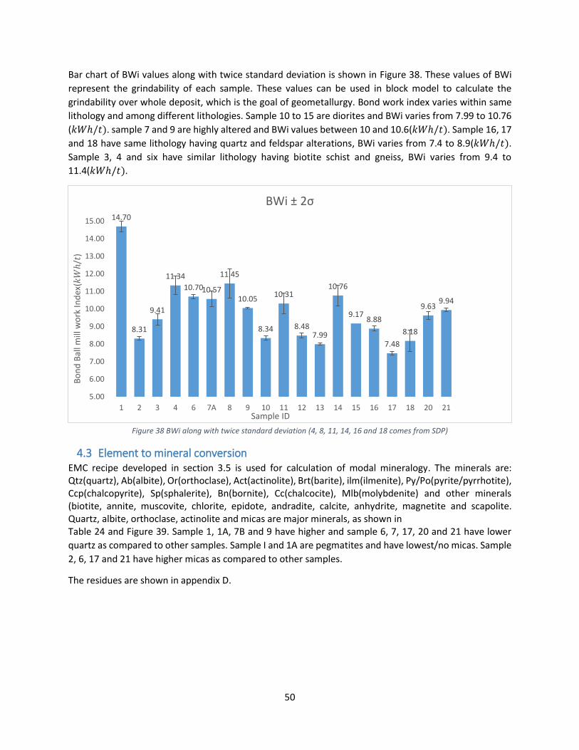
50

Bar chart of BWi values along with twice standard deviation is shown in Figure 38. These values of BWi

represent the grindability of each sample. These values can be used in block model to calculate the

grindability over whole deposit, which is the goal of geometallurgy. Bond work index varies within same

lithology and among different lithologies. Sample 10 to 15 are diorites and BWi varies from 7.99 to 10.76

(𝑘𝑊ℎ/𝑡). sample 7 and 9 are highly altered and BWi values between 10 and 10.6(𝑘𝑊ℎ/𝑡). Sample 16, 17

and 18 have same lithology having quartz and feldspar alterations, BWi varies from 7.4 to 8.9(𝑘𝑊ℎ/𝑡).

Sample 3, 4 and six have similar lithology having biotite schist and gneiss, BWi varies from 9.4 to

11.4(𝑘𝑊ℎ/𝑡).

Figure 38 BWi along with twice standard deviation (4, 8, 11, 14, 16 and 18 comes from SDP)

4.3 Element to mineral conversion EMC recipe developed in section 3.5 is used for calculation of modal mineralogy. The minerals are: Qtz(quartz), Ab(albite), Or(orthoclase), Act(actinolite), Brt(barite), ilm(ilmenite), Py/Po(pyrite/pyrrhotite), Ccp(chalcopyrite), Sp(sphalerite), Bn(bornite), Cc(chalcocite), Mlb(molybdenite) and other minerals (biotite, annite, muscovite, chlorite, epidote, andradite, calcite, anhydrite, magnetite and scapolite. Quartz, albite, orthoclase, actinolite and micas are major minerals, as shown in Table 24 and Figure 39. Sample 1, 1A, 7B and 9 have higher and sample 6, 7, 17, 20 and 21 have lower

quartz as compared to other samples. Sample I and 1A are pegmatites and have lowest/no micas. Sample

2, 6, 17 and 21 have higher micas as compared to other samples.

The residues are shown in appendix D.

14.70

8.31

9.41

11.34

10.7010.57

11.45

10.05

8.34

10.31

8.487.99

10.76

9.178.88

7.48

8.18

9.639.94

5.00

6.00

7.00

8.00

9.00

10.00

11.00

12.00

13.00

14.00

15.00

1 2 3 4 6 7A 8 9 10 11 12 13 14 15 16 17 18 20 21

Bo

nd

Bal

l mill

wo

rk In

dex

(𝑘𝑊

ℎ/𝑡

)

Sample ID

BWi ± 2σ

51

Figure 39 Modal Mineralogy of Aitik mine samples calculated by EMC

Table 24: EMC modal minerology of Aitik Mine samples

ID Qtz % Ab % Or % Act % Brt % Ilm % (Py+Po)

% Ccp % Sp % Bn % Cc % Mlb % Other

Minerals

1 37.52 39.29 23.65 0.61 0.23 0.12 0.00 0.03 0.01 0.00 0.00 0.00 0.00

1A 39.89 33.76 24.59 0.00 0.43 0.10 0.00 0.02 0.00 0.00 0.00 0.00 1.22

2 29.27 25.27 5.72 2.96 0.11 1.57 0.00 0.02 0.01 0.00 0.00 0.00 35.08

3 21.23 29.28 22.87 0.00 1.42 1.08 3.64 0.41 0.01 0.00 0.00 0.00 20.08

6 16.18 25.38 19.74 1.78 0.26 1.83 3.20 0.49 0.01 0.00 0.00 0.00 31.15

7 13.70 40.84 7.63 9.92 0.44 1.60 0.19 0.27 0.01 0.00 0.00 0.00 25.42

7B 30.39 17.94 21.44 0.00 0.75 0.99 0.56 1.18 0.01 0.00 0.00 0.00 26.74

9 30.65 12.52 24.79 0.00 0.64 0.97 0.00 1.25 0.01 0.00 0.00 0.00 29.18

10 22.76 34.87 11.45 10.45 0.15 1.00 0.15 0.17 0.01 0.00 0.00 0.00 19.01

12 21.99 42.38 3.37 11.45 0.16 1.08 0.32 0.38 0.01 0.00 0.00 0.00 18.85

13 22.39 39.96 4.71 13.77 0.22 1.05 0.20 0.24 0.01 0.00 0.00 0.00 17.46

15 17.65 38.19 9.02 9.36 0.25 1.11 0.16 0.20 0.00 0.00 0.00 0.00 24.06

17 8.89 30.80 0.00 23.73 0.25 1.78 1.01 0.45 0.01 0.00 0.00 0.00 33.09

20 12.01 44.14 2.72 14.31 0.12 1.42 0.00 0.03 0.02 0.00 0.00 0.00 25.25

21 11.90 28.85 20.74 0.00 0.31 1.82 0.74 0.77 0.04 0.00 0.00 0.00 34.86

The average standard deviation of modal mineralogy calculated by monte carlo simulation is shown in

Table 25. Monte carlo simulation used the default value of standard deviation (4%) in chemical assays.

0%

10%

20%

30%

40%

50%

60%

70%

80%

90%

100%

1 1A 2 3 6 7 7B 9 10 12 13 15 17 20 21

Mo

dal

min

ero

logy

Sample ID

EMC Modal Minerology

Qtz % Ab % Or % Act % Brt % Ilm % (Py+Po) % Ccp % Sp % Bn % Cc % Mlb % other minerals

52

After fifty rounds the average standard deviation was calculated. Quartz has a higher standard deviation

because quartz is calculated on basis of remaining sulfur and sulfur is present in most of the minerals.

Molybdenite has zero standard deviation because of low quality and molybdenum was unique mineral for

calculation of molybdenite. The lower standard deviation for chalcopyrite, pyrite and pyrrhotite show

good results from EMC. The standard deviation for chalcocite and bornite is zero because all copper was

taken by chalcopyrite and these minerals were in very low quantity and counts in SEM results.

Table 25 Average Standard deviation calculated by Monte carlo Simulation in HSC software

Sample ID

Qtz Ab Or Act Brt Ilm (Py+Po) Ccp Sp Bn Cc Mlb Other

Minerals

± % ± % ± % ± % ± % ± % ± % ± % ± % ± % ± % ± % ± %

1 3.50 1.94 2.82 0.00 0.02 0.00 0.00 0.00 0 0 0 0 4.35

1A 2.26 1.34 2.30 0.91 0.01 0.08 0.00 0.00 0 0 0 0 2.88

2 2.85 1.18 2.79 0.00 0.16 0.22 0.74 0.03 0 0 0 0 4.23

3 2.42 1.18 4.48 1.38 0.02 0.12 0.20 0.03 0 0 0 0 5.38

6 2.31 1.82 2.40 1.18 0.02 0.10 0.00 0.02 0 0 0 0 3.13

7 2.94 0.75 1.98 0.00 0.05 0.05 0.08 0.07 0 0 0 0 3.43

7A 3.07 0.99 2.82 0.00 0.05 0.05 0.10 0.06 0 0 0 0 3.83

8 2.57 0.55 2.52 0.00 0.04 0.05 0.04 0.07 0 0 0 0 3.36

9 2.57 1.72 2.36 0.68 0.01 0.05 0.02 0.01 0 0 0 0 2.83

10 2.85 2.54 2.32 0.94 0.01 0.06 0.03 0.02 0 0 0 0 3.35

12 3.28 1.94 2.48 0.92 0.01 0.06 0.02 0.02 0 0 0 0 4.17

13 3.11 1.28 2.70 0.68 0.03 0.28 0.00 0.01 0 0 0 0 4.60

15 2.46 11.64 0.00 1.79 0.01 0.09 0.06 0.02 0 0 0 0 3.00

17 3.66 2.20 2.09 1.54 0.01 0.48 0.00 0.00 0 0 0 0 5.26

20 2.68 1.18 7.02 0.44 0.02 0.09 0.08 0.05 0 0 0 0 6.71

21 0.00 0.00 0.00 0.00 0.00 0.00 0.00 0.00 0 0 0 0 0.00

4.4 Regrinding circuit Aitik (Pebble mill) To plot particle size distribution of regrinding samples, sieving was used. Dry sieving was used in the

laboratory with minimum sieve size of 75µm and highest sieve size of 212µm with 106 µm, 150µm

intermediate sieves. In Figure 40, it is easy to observe that the overflow of the hydrocyclone has fine

particle size distribution while underflow of the hydrocyclone has coarse particle size distribution. Mill

product has more coarse and less fine particles as compared to the rougher concentrate. The reason is

the recirculation of underflow of the hydrocyclone to the mill. Underflow of hydrocyclone has coarser size

distribution and high solid flowrate as compared to rougher concentrate.

53

Figure 40 Particle size distribution of Aitik regrinding circuit

4.5 Automated mineralogy results of regrinding circuit

4.5.1 Modal mineralogy Modal Mineralogy of Rougher concentrate is shown in Figure 41. Rougher concentrate has 69.5% pyrite,

21% chalcopyrite and 10% other minerals. There is low pyrite and higher chalcopyrite in size fraction 150-

425µm as compared to other size fractions. Mill product has 75.8% pyrite, 15.9% chalcopyrite and 8%

other minerals roughly, shown in Figure 42. Size fraction 106-212µm has higher chalcopyrite and lower

pyrite in mill product. Underflow of hydrocyclone has 81.5% pyrite, 13.4% chalcopyrite and 5% other

minerals roughly, shown in Figure 43. Size fraction 75-106µm has higher pyrite and size faction 150-425

µm has higher chalcopyrite in hydrocyclone underflow. Overflow has 61.5% pyrite, 22.5% chalcopyrite

and 16% other minerals roughly, shown in Figure 44. Size fraction 106-150µm has higher chalcopyrite and

size fraction 150-212 µm has lower pyrite in hydrocyclone overflow.

Underflow of hydrocyclone is recirculated to the mill for re-grinding along with rougher concentrate.

Underflow is recirculating around 82% pyrite and 13% chalcopyrite to the mill.

0

0.2

0.4

0.6

0.8

1

1.2

0 50 100 150 200 250

cum

ula

ted

mas

s p

ass

Sieve size (micron)

Particle size distribution

Over Flow HC

Under-Flow HC

Rougher Conc.

Mill Product

54

Figure 41 Modal mineralogy of rougher concentrate

Figure 42 Modal mineralogy of mill product

0

20

40

60

80

100

Bulk 0-75 75-106 106-150 150-425

Wei

ght

per

cen

t m

iner

al (

%)

Size fraction (µm)

Modal mineralogy of rougher Conc.

Quartz

Mica

Chalcopyrite

Fe-Oxides

Feldspar

Pyrite

other sulphides

silicates

other minerals

0

20

40

60

80

100

Bulk 0-75 75-106 106-212 212-425

Wei

ght

per

cen

t m

iner

al (

%)

Size fraction (µm)

Modal mineralogy of mill product

Quartz

Mica

Chalcopyrite

Fe-Oxides

Feldspar

Pyrite

othersulphides

55

Figure 43 Modal mineralogy of hydrocyclone underflow

Figure 44 Modal mineralogy of hydrocyclone overflow

4.5.2 Liberation analysis Liberation graph of chalcopyrite is shown in Figure 45. Chalcopyrite is highly liberated in size faction 75-

106µm. Size fraction 150-425µm have higher binary chalcopyrite with pyrite and micas. Around 5%

chalcopyrite in size factions 75-106µm and 106-50µm is binary with micas. Size faction 0-75µm shows

over estimation of binary chalcopyrite due to agglomeration and presence of ultra-fine particles.

0

20

40

60

80

100

Bulk 0-75 75-106 106-150 150-425

Wei

ght

per

cen

t m

iner

al (

%)

Size fraction (µm)

Modal mineralogy of HC-UnderflowQuartz

Mica

Chalcopyrite

Fe-Oxides

Feldspar

Pyrite

othersulphidessilicates

0

20

40

60

80

100

Bulk 0-75 75-106 106-150 150-212 212-425

Wei

ght

per

cen

t m

iner

al (

%)

Size fraction (µm)

Modal mineralogy of HC-Overflow

Quartz

Mica

Chalcopyrite

Fe-Oxides

Feldspar

Pyrite

othersulphidessilicates

other minerals

56

Figure 45 Mode of occurrence of chalcopyrite in rougher concentrate

Liberation data of chalcopyrite in mill product is shown in Figure 46. Size fraction 0-75µm shows

underestimation of liberated chalcopyrite. In size fraction 75-106µm, results are strange, since this

fraction has no ultra-fine particles but still it shows underestimation of liberated chalcopyrite, one reason

could be the lower number of particles in this size fraction. Size fraction 106-212 and 212-425µm shows

good liberation of chalcopyrite.

Figure 46 Mode of occurrence of chalcopyrite in Mill product

57

Liberation data of chalcopyrite in hydrocyclone overflow is shown in Figure 47. The highest liberated

chalcopyrite is in size fraction 106-150µm. Chalcopyrite in hydrocyclone overflow is binary and tertiary

with other minerals, binary and tertiary particles of chalcopyrite get lower densities, hence recovered in

overflow. Size fraction 0-75µm also shows underestimation of liberated chalcopyrite due to

agglomeration and presence of ultra-fine particles.

Figure 47 Liberation graphs of chalcopyrite in Hydrocyclone overflow

Liberation results of chalcopyrite in hydrocyclone underflow are shown in Figure 48. It can be analyzed

that most of the chalcopyrite in underflow is liberated. Binary chalcopyrite with pyrite and mica is present

58

in some size fractions. Size fraction 0-75µm shows under estimation of liberated chalcopyrite because of

agglomeration and presence of ultra-fine particles, shown in figure 48.

Figure 48 Liberation data of chalcopyrite in hydrocyclone underflow

4.5.3 Ultra fine particules in fraction 0-75µ Size fraction 0-75 microns have underestimation of liberated particles and overestimated of non-liberated

particles because of segregation and presence of ultra-fine particles. A group of particles was considered

as single particles by SEM, can be seen in Figure 49. Density segregation during preparation of polished

section is most difficult to avoid and detect (Kwitko-Ribeiro 2011). Very fine particles are making

connection between bigger particles because of which a group of particles was taken as single particle by

SEM, hence overestimation of non-liberated and underestimation of liberated particles.

59

Figure 49 particles in fraction 0-75µm

4.6 Classification of samples

4.6.1 Classification based on bond work Index We can classify Aitik samples into different classes based on BWi values. Using Table 3, Aitik samples can

be classified into soft (7-9 𝑘𝑊ℎ/𝑡), medium (9-14 𝑘𝑊ℎ/𝑡) and hard (14-20 𝑘𝑊ℎ/𝑡) rocks. Classification

is shown in Table 26. Sample 2, 10, 12, 13, 16, 17 and 18 (mostly diorites and foot-wall) are classified as

soft samples. Sample 3, 4, 6, 7A, 8, 9, 11, 14, 15, 20 and 21 (ore zone and diorites) are classified as medium

samples. Sample 1 is classified as hard sample.

Table 26: Classification of samples based on BWi values

Soft (BWi 7-9 𝒌𝑾𝒉/𝒕) Medium (BWi 9-14 𝒌𝑾𝒉/𝒕) Hard (BWi>14 𝒌𝑾𝒉/𝒕)

Sample ID. Mean BWi (𝒌𝑾𝒉/𝒕)

Sample ID.

Mean BWi (𝒌𝑾𝒉/𝒕)

Sample ID. Mean BWi (𝒌𝑾𝒉/𝒕)

2 8.31 3 9.41 1 14.70

10 8.34 4 11.34 12 8.48 6 10.70 13 7.99 7A 10.57 16 8.88 8 11.45 17 7.48 9 10.05 18 8.18 11 10.31

14 10.76

15 9.17

20 9.63

21 9.94

60

4.6.2 Principal component analysis Principle component analysis is used to reduce the dimensions and classification of data. The larger

number of variables are replaced by smaller number called principle components which are linear

combination of the original variables. The first PC is obtained in the direction of maximum variability in

the data set. The second PC is the orthogonal to the first PC covering the second highest variability in the

data set and so on. The original variables are converted into lower number of principle components and

maximum variability in the dataset is covered (Jolliffe, 2002).

Here, the purpose of principle analysis was to reduce the dimensions of data and classify samples into

different ore types. The input data for PCA is the modal mineralogy of the Aitik mine samples calculated

by EMC. The minerals are: Qtz(quartz), Ab(albite), Or(orthoclase), Act(actinolite), Brt(barite),

ilm(ilmenite), Py/Po(pyrite/pyrrhotite), Ccp(chalcopyrite), Sp(sphalerite), Bn(bornite), Cc(chalcocite),

Mlb(molybdenite) and other minerals (biotite, annite, muscovite, chlorite, epidote, andradite, calcite,

anhydrite, magnetite and scapolite).

The correlation matrix is shown in Table 27. Where Pearson correlation coefficient is calculated between

each entity.

Table 27: Correlation matrix (Pearson (n)):

Variables Bwi Qtz % Ab % Or % Act % Brt % Ilm % (Py+Po)

% Ccp % Sp % Other

Minerals

Bwi 1 0.456 0.051 0.639 -0.561 0.067 -0.508 0.008 -0.050 0.073 -0.560

Qtz % 0.456 1 -0.232 0.443 -0.533 0.060 -0.787 -0.240 -0.041 -0.338 -0.569

Ab % 0.051 -0.232 1 -0.551 0.508 -0.348 -0.209 -0.289 -0.733 -0.072 -0.513

Or % 0.639 0.443 -0.551 1 -0.869 0.533 -0.331 0.396 0.498 0.197 -0.201

Act % -0.561 -0.533 0.508 -0.869 1 -0.411 0.232 -0.291 -0.317 -0.216 0.079

Brt % 0.067 0.060 -0.348 0.533 -0.411 1 -0.108 0.645 0.366 -0.064 -0.045

Ilm % -0.508 -0.787 -0.209 -0.331 0.232 -0.108 1 0.280 0.187 0.373 0.901

(Py+Po) % 0.008 -0.240 -0.289 0.396 -0.291 0.645 0.280 1 0.174 -0.012 0.151

Ccp % -0.050 -0.041 -0.733 0.498 -0.317 0.366 0.187 0.174 1 0.277 0.405

Sp % 0.073 -0.338 -0.072 0.197 -0.216 -0.064 0.373 -0.012 0.277 1 0.315

Other Minerals -0.560 -0.569 -0.513 -0.201 0.079 -0.045 0.901 0.151 0.405 0.315 1

Figure 50 shows the cumulative variability coved by factors (new derived dimensions) calculated in PCA.

Where 100% variability was covered by 10 possible factors which is difficult to interpret. We can take only

some factors which cover the large amount of variability in the data. Factor 1 and factor 2 covered around

69% of variability inside dataset. While first three factors covered around 81 % of the variability in the

data. For classification of data we used first two factors which covered 69% variability in the data.

61

Figure 50 Cumulative variability of factors

Figure 51 shows the contribution of minerals and BWi to the first two factors. Factor 1 and Factor 2 were

derived from linear combination modal mineralogy. Quartz and orthoclase were contributing positively

to the factor 1. Actinolite, ilmenite, albite and other minerals were contributing negatively to the factor

one. Ilmenite, chalcopyrite and other minerals were contributing positively to the factor 2. Albite, quartz

and actinolite were contributing negatively to the factor 2.

Figure 51 Contribution of different properties to the first two factors.

Figure 52 shows the position of each sample on the factors plot. Figure 52 can be used to classify the data,

based on first two factors which cover 69% variability in the data. We can observe in Figure 53, the position

0

20

40

60

80

100

0

0.5

1

1.5

2

2.5

3

3.5

4

4.5

F1 F2 F3 F4 F5 F6 F7 F8 F9 F10

Cu

mu

lati

ve

va

ria

bil

ity %

)

Eig

en

va

lue

axis

Scree plot

Qtz %

Ab %

Or %

Act %

Brt %

Ilm %(Py+Po) %

Ccp %

Sp %

Other Minerals

-1

-0.75

-0.5

-0.25

0

0.25

0.5

0.75

1

-1 -0.75 -0.5 -0.25 0 0.25 0.5 0.75 1

F2

(2

9,6

8 %

)

F1 (39,67 %)

Variables (axes F1 and F2: 69,35 %)

62

of different samples on factors plot and the clustering of samples. Sample 1 and 1A shows a high value of

quartz. Sample 1 and 1A seems alone having high BWi since these samples are identified as pegmatites.

Where sample 3, 9, 4, 8 and 7b has high contribution of orthoclase, barite, pyrite and chalcopyrite, with

lower contribution of albite and actinolite. These samples also have medium to higher value of quartz.

Sample 16, 17 and 18 have high contribution of actinolite and lower quartz. Sample 6 and 21 have higher

contribution of either pyrite or chalcopyrite. There is a big cluster of sample 10, 11, 12, 13, 14 and 15 near

origin of the graph. This cluster shows lower contribution both factors. Sample 7 and 20 have same

mineralogy as sample 2. Sample 20 have higher actinolite.

Figure 52 Contribution of different properties to the first two factors along with the samples

1

2

3

6

7

9

1012

13

15

17

20

21

4 8

11

14

1618

1A

7B

Qtz %

Ab %

Or %

Act %

Brt %

Ilm %(Py+Po) %

Ccp %

Sp %

Other Minerals

-4

-3

-2

-1

0

1

2

3

4

-5 -4 -3 -2 -1 0 1 2 3 4 5 6

F2

(2

9,6

8 %

)

F1 (39,67 %)

Biplot (axes F1 and F2: 69,35 %)

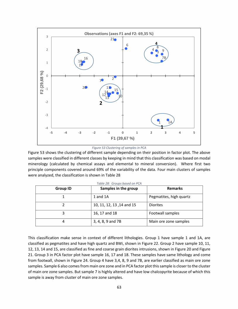
63

Figure 53 Clustering of samples in PCA

Figure 53 shows the clustering of different sample depending on their position in factor plot. The above

samples were classified in different classes by keeping in mind that this classification was based on modal

minerology (calculated by chemical assays and elemental to mineral conversion). Where first two

principle components covered around 69% of the variability of the data. Four main clusters of samples

were analyzed, the classification is shown in Table 28

Table 28: Groups based on PCA

Group ID Samples in the group Remarks

1 1 and 1A Pegmatites, high quartz

2 10, 11, 12, 13 ,14 and 15 Diorites

3 16, 17 and 18 Footwall samples

4 3, 4, 8, 9 and 7B Main ore zone samples

This classification make sense in context of different lithologies. Group 1 have sample 1 and 1A, are

classified as pegmatites and have high quartz and BWi, shown in Figure 22. Group 2 have sample 10, 11,

12, 13, 14 and 15, are classified as fine and coarse grain diorites intrusions, shown in Figure 20 and Figure

21. Group 3 in PCA factor plot have sample 16, 17 and 18. These samples have same lithology and come

from footwall, shown in Figure 24. Group 4 have 3,4, 8, 9 and 7B, are earlier classified as main ore zone

samples. Sample 6 also comes from main ore zone and in PCA factor plot this sample is closer to the cluster

of main ore zone samples. But sample 7 is highly altered and have low chalcopyrite because of which this

sample is away from cluster of main ore zone samples.

1

2

3

6

7

9

101213

15

17

20

21

48

1114

1618

1A

7B

-4

-3

-2

-1

0

1

2

3

-5 -4 -3 -2 -1 0 1 2 3 4 5

F2

(2

9,6

8 %

)

F1 (39,67 %)

Observations (axes F1 and F2: 69,35 %)

4

3

2

1

64

PCA indicate that the mineralogy of footwall, main ore zone, pegmatites and diorites is significantly

different because of which we can see clear cluster of similar ore type sample.

5 Conclusions Comminution tests are important in context of geometallurgy for making proper geometallurgical process

models, production planning and management. In this study, different comminution methods were

reviewed to find a suitable comminution test method. Geometallurgical comminution test method was

used to estimate the bond work index for Aitik’s samples. In literature review some good correlations

were found between different comminution tests methods which are useful for conversion between

different indices.

BWi values varies from 7.48 [𝑘𝑊ℎ/𝑡] and 14.7[𝑘𝑊ℎ/𝑡]. Sample 13 has minimum BWi value of

7.48[𝑘𝑊ℎ/𝑡] among all samples. Sample 1 (pegmatite) has highest value of 14.7 [𝑘𝑊ℎ/𝑡] because of

presence of highest quartz as compared to other samples. Main ore zone has less grindability (high BWi)

as compared to diorites, hanging wall and footwall because of presence of medium to high value of quartz.

Footwall has highest grindability which indicate and footwall is weaker as compared to ore zone and

hanging wall. Footwall has lower quartz and higher micas (other minerals). These values of grindability

can be used in future study for mapping of grindability over whole deposit. Which will be useful for Aitik

to better optimize and manage the comminution circuit.

Element to mineral conversion gave good results for calculation of modal mineralogy of Aitik ore. The modal mineralogy calculated by element to mineral conversion was compared with modal mineralogy calculated by automated mineralogy for same samples. Results indicated that the 𝑅2 value for quartz, chalcopyrite, albite, orthoclase, actinolite, (pyrite+ pyrrhotite), and barite were 0.84, 0.85, 0.87, 0.65, 0.77, 0.74 and 0.6 respectively. These 𝑅2 values are not really good but still there is a strong correlation between modal mineralogy of element to mineral conversion and automated mineralogy. Correlations were found between BWi and modal mineralogy. Multiple linear regression was used to predict the BWI values. Results indicated that the selected minerals have covered 57% variance of BWi. This model gave RMSE of 0.948[𝑘𝑊ℎ/𝑡] with P value of 0.048 showing that model was effective and there was less than 5% probability that the results from this modal are random. Multiple linear regression in main ore zone samples provides good results by covering of 98.7% variability in BWI by the selected minerals. The RMSE values is 0.222 [𝑘𝑊ℎ/𝑡] with p value of 0.026. Modelling of BWi in diorites are gave good results but there is a chance of multicollinearity between the data, where 95% variance of BWi is covered with RMSE of 0.4 [𝑘𝑊ℎ/𝑡] and p value of 0.025. Multiple linear regression gives more good prediction of BWi in different type of ore, instead of modelling of BWi on whole deposit Principle component analysis classified Aitik mine samples into different classes based on modal mineralogy. This classification was based on scatter plot of first two factors which covered 69 percent variance of data. Groups are; pegmatites, diorites, main ore zone and foot wall, showing the significant difference in their mineralogy. It is concluded from liberation analysis of Aitik regrinding circuit that the rougher concentrate already has good liberation of chalcopyrite. Rougher concentrate also has binary particles of chalcopyrite-micas and chalcopyrite-pyrite. Hydrocyclone underflow (in regrinding circuit) is recirculating around 82% pyrite to the re-grinding mill, containing binary particles of chalcopyrite-pyrite and chalcopyrite-micas. When we put element to mineral conversion, models from linear regression and principle component analysis together, we can conclude that the elemental assays can be used to calculate modal mineralogy using recipe made in element to mineral conversion. Element to mineral conversion results can further be used in principle component analysis to classify sample into proper ore type and select the proper

65

multiple linear regression model for prediction of BWi. Then selected model from linear regression can be used to predict the BWi value for that sample. By following this whole path, the elemental assays will end up in grindability information of the samples.

5.1 Future work

• Integration of comminution data with geology, recovery data and resource model to get a global

domain which will be more effective for mine planning and mill design.

• The available comminution information (BWi) can be used in a spatial model to make

geometallurgical comminution domains. Variograms and kriging can be used for interpolation of

BWi over whole deposit, which will end up in a block model which fits more in mining

environment. Since location of all Aitik mine samples were confidential for this study but in future

before spatial study the sampling should be statistically verified (enough number of samples for

being representative) to be used in block model. For current study, there are only 21 samples

having BWi values, are not enough to represent whole deposit in term of comminution so there

is a need for further sample collection for measurement of BWi. There are two possibilities for

measurement of BWi: first is the use of GCT to calculate BWi for all new samples, second is the

use of EMC and models from linear regressions to predict BWi values for all new samples (EMC --

Modal mineralogy –linear regression models). Once there are enough number of representative

samples, we can go for spatial models (variograms, kriging, wireframe domains and block models)

to map the comminution variability over whole deposit and can make geometallurgical

comminution domains.

• The available comminution information is in form of bond ball mill work index (BWi) but Aitik has

AG/SAG mills in their grinding circuits and BWi is mostly used for modelling and sizing of ball mills.

In context of mapping and comparison of comminution properties, bond work index can be used.

But when it comes to the modelling (throughput, PSD, energy requirement) of AG/SAG mills, we

need AG/SAG mill comminution tests. There are two ways to get these information: First way is

to find out the possible correlations between BWi and indices from AG/SAG comminution tests

(as discussed in literature review, section 2.6) and then converting BWi values into other AG/SAG

indices using the linear models, coming from linear fitting of their scatter plots. For this modelling,

there is a requirement of calculation of AG/SAG indices and BWi for same samples. The second

way is to do separate comminutions tests for AG/SAG mill. Comminution tests for AG/SAG mill

will be a sort of extensive work (because of sample size, cost and time), as shown in Table 29.

There is a suggested solution to reduce this work by making spatial geometallurgical comminution

domains using BWi and then running couple of SAG/AG comminution tests in each comminution

domain to get this information over whole deposit. So, in this case we can go with both AG/SAG

comminution indices and BWi. Verret et al. (2011) made a comparison of details of all

commminution test methods for AG/SAG mill, shown in Table 29.

66

Table 29 SAG/AG mill comminution test methods (Verret et al. 2011)

5.2 Recommendations

• Collection of more samples for BWi measurements for better representation of the deposit.

• Study of mineral composition to improve element to mineral conversion.

• EMC may give good results if done in each zone (classification results from PCA) separately.

• Standard deviation of chemical assays should be used in monte carlo simulation in HSC software for calculate the possible error in calculated modal mineralogy (the error which results due to the standard deviation of chemical assays).

• For multiple linear regression in each ore type, more samples should be collected for better modelling of BWi with higher confidence level.

• Use of geological data in PCA to get better geological domains.

• Use of wet sieving for -75µm fraction (for all samples) to remove fines and split this fraction into sub-fractions (in overflow 65% particles by weight are in this size fraction). Size fraction 75-106µm in mill product showed underestimation of liberated minerals, this sample should be prepared and restudied n SEM.

67

6 References Aiken LS, West SG, Pitts SC (2003) Multiple linear regression. Alruiz OM, Morrell S, Suazo CJ, Naranjo A (2009) A novel approach to the geometallurgical modelling of

the Collahuasi grinding circuit. Miner Eng 22:1060–1067. doi: 10.1016/j.mineng.2009.03.017 Alvarado S, Alguerno J, Auracher H, Casali A (1998) Energy and Exergy Optimization of Comminution.

Energy 23:153–158. Bachman WD, Last AW, Nabbs SW (1970) Autogenous grinding of disseminated copper ores. TRANS SOC

Min ENG AIME 247:251–255. Barratt DJ, Matthews BD, deMull T (1996) Projection of AG/SAG mill sizes, mill speeds, ball charges and

throughput variation from Bond work indices. Proc Int autogenous semiautogenous Grind Technol 2:541–558.

Boliden (2014) Annual Report 2014. Boliden (2016) Boliden ’ s mineral reserves and resources 2016.

http://www.boliden.com/globalassets/bolidens-mineral-reserves-2016_eng.pdf. Bond FC (1961) Crushing and grinding calculations. Allis-Chalmers Manufacturiing Company Bond FC (1952) The 3rd theory of comminution. Trans Am Inst Min Metall Eng 193:484–494. Bond FC (1949) Standard Grindability Tests Tabulated. Trans Am Inst Min Metall Eng 183:313–329. Cargill JS, Shakoor A (1990) Evaluation of empirical methods for measuring the uniaxial compressive

strength of rock. Int J Rock Mech Min Sci Geomech Abstr 27:495–503. doi: 10.1016/0148-9062(90)91001-N

Dobby G, Bennett C, Kosick G (2001) Advances in SAG circuit design and simulation applied: The mine block model. Proc Int autogenous semiautogenous Grind Technol 4:221–234.

Drzymala J (2007) Mineral Processing, Foundations of theory and practice of minerallurgy. Ergün Tuncay NH (2009) The effect of length to diameter ratio of test specimens on the uniaxial

compressive strength of rock. F.O. VERRET GCAAM (2011) SAG MILL TESTING - AN OVERVIEW OF THE TEST PROCEDURES AVAILABLE TO

CHARACTERIZE ORE GRINDABILITY. Haffez GSA (2012) Correlation between work index and mechanical properties of some Saudi Ores. Mater

Test 54:108–112. Harbort GJ, Lam K, Sola C (2013) The use of Geometallurgy to Estimate Comminution Parameters within

Porphyry Copper Deposits. 217–230. Hunt J, Kojovic T, Berry R (2013) Estimating Comminution Indices from Ore Mineralogy , Chemistry and

Drill Core Logging. 173–176. JKTech (1992) JK Drop Weight Test in detail. 7–9. Kaiser M a, Dr. Alfred Wicks, Leonard Wilson, Dr. William Saunders (1998) Advancements in the Split

Hopkinson Bar Test. Mech Eng Master:94. Keeney L, La Montoya P, Montoya PA, et al (2011) Geometallurgical Modelling Applicable to Pre

Techniques Applicable to Prefeasibility Projects – La Colosa Case Study. Keeney L, Walters SG (2011) A Methodology for Geometallurgical Mapping and Orebody Modelling

COMMON PROBLEMS IN CURRENT. 5–7. King RP (2012) Modeling and simulation of mineral processing systems. Elsevier Kwitko-Ribeiro R (2011) New sample preparation developments to minimize mineral segregation in

process mineralogy. … 10th Int Congr Appl Mineral … 1–5. doi: 10.1007/978-3-642-27682-8 Lamberg P (2011) Particles–the bridge between geology and metallurgy. In: Proceedings of the

Conference in Minerals Engineering, Luleå, Sweden. Citeseer, pp 8–9 Levin J (1989) Observations on the Bond standard grindability test , and a proposal for a standard

grindability test for fine materials. J South African Inst Min Metall 89:13–20. doi: 10.1016/0148-

68

9062(89)91143-1 Li D, Wong LNY (2013) The brazilian disc test for rock mechanics applications: Review and new insights.

Rock Mech Rock Eng 46:269–287. doi: 10.1007/s00603-012-0257-7 MacPherson AR, Turner RR (1978) Autogenous grinding from test work to purchase of a commercial unit.

Miner Process plant Des 279–305. Magdalinovic N (1989) A procedure for rapid determination of the Bond work index. Int J Miner Process

27:125–132. doi: 10.1016/0301-7516(89)90010-0 Mcken A, Williams S (2005) An Overview of the Small-scale Tests Available to Characterize Ore Grindability

for Design Purposes. SGS Miner Tech Bull 2005:8. Mwanga A, Lamberg P, Rosenkranz J (2015) Comminution test method using small drill core samples.

Miner Eng. doi: 10.1016/j.mineng.2014.12.009 Narayanan SS (1985) Development of a laboratory single particle breakage technique and its application

to ball mill modelling and scale-up. The University of Queensland Ozkahraman HT (2005) A meaningful expression between bond work index, grindability index and friability

value. Miner Eng 18:1057–1059. doi: 10.1016/j.mineng.2004.12.016 Parian M, Lamberg P, Möckel R, Rosenkranz J (2015) Analysis of mineral grades for geometallurgy:

Combined element-to-mineral conversion and quantitative X-ray diffraction. Miner Eng. doi: 10.1016/j.mineng.2015.04.023

Rod B, Index M, Brmwi T (1961) JKTech Laboratory Services. 6:6–7. Rusnak J, Mark C (2000) Using the Point Load Test To Determine the Uniaxial Compressive Strength of

Coal Measure Rock. 19th Int Conf Gr Control Mining, 8-10 August 362–371. Sahoo RK, Weedon DM, Roach D (2004) Single-particle breakage tests of Gladstone Port Authority ’ s coal

by a twin pendulum apparatus. Adv Powder Technol 15:263–280. doi: 10.1163/156855204773644472

Sammelin M, Wanhainen C, Martinsson O (2011) Gold mineralogy at the Aitik Cu – Au– Ag deposit, Gällivare area, northern Sweden. GFF 133:19–30.

Schönert K, Marktscheffel M (1986) Liberation of composite particles by single particle compression, shear and impact loading. In: Proceedings of the 6th European Symposium Comminution, Nürnberg, Germany. pp 16–18

Starkey J, Dobby G (1996) Application of the Minnovex Sag Power Index At Five Canadian Sag Plants. Autogenous Semi-Autogenous Grind 345–360.

States U, Efficiency E, Energy R (2004) Industrial Technologies Program — Boosting the Productivity and Competitiveness of U . S . Industry.

Swain R, Rao RB (2009) Alternative Approaches for Determination of Bond Work Index on Soft and Friable Partially Laterised Khondalite Rocks of Bauxite Mine Waste Materials. 8:729–743.

Tavares LM (1999) Energy Absorbed in Breakage of Single Particles in Drop Weight Testing. Miner Eng 12:43–50.

USGS (2008) Preliminary Model of Porphyry Copper Deposits. Wanhainen C (2005) On the Origin and Evolution of the Palaeoproterozoic Aitik Cu-Au-Ag Deposit,

Northern Sweden. Wanhainen C (2003) Copper and gold distribution at the Aitik Deposit, Gällivare Area, Northern Sweden.

Trans Inst Min Metall Sect B Appl Earth Sci 112:260–267. doi: 10.1179/037174503225011289 Weichert R, Herbst JA (1986) An ultra fast load cell device for measuring particle breakage. In: 1st World

Congress of Particle Technology. Nürnberg. Whiten B (2007) CALCULATION OF MINERAL COMPOSITION FROM CHEMICAL ASSAYS. Miner Process Extr

Metall Rev 29:83–97. doi: 10.1080/08827500701257860 Zweifel H (1976) Aitik-geological documentation of a disseminated copper deposit: a preliminary

investigation. SGU

69

7 Appendices

4.7 Appendix A Particle Size distributions:

Sample 1:

Figure 54 Particle Size distribution at different grinding times

Figure 55 Standard deviation based on two repeats at different grinding times

0.0%

20.0%

40.0%

60.0%

80.0%

100.0%

120.0%

10 100 1000 10000

Acc

um

ula

ted

per

cen

t m

ass

pas

s

Sieve sizes (microns)

Particle Size distribution

0 Min.

2-Min.

5 Min

8 Min.

11 Min.

0.00%

0.10%

0.20%

0.30%

0.40%

0.50%

840 425 212 106 75 0

Stan

dar

d D

evia

tio

n

Sieve Size

Standard Deviation (%)Time 0 MIn

Time 2 Min.

Time 5 Min

Time 8 Min

Time 11Min

70

Sample 2:

Figure 56 Particle Size distribution at different grinding times

Figure 57 Standard deviation based on two repeats at different grinding times

Sample 3:

0.0%

20.0%

40.0%

60.0%

80.0%

100.0%

120.0%

10 100 1000 10000

Acc

um

ula

ted

per

cen

t m

ass

pas

s

Sieve Sizes (micron)

Particle size distribution

0 Min.

2-Min.

5 Min

8 Min.

0.00%

0.20%

0.40%

0.60%

0.80%

1.00%

1.20%

840 425 212 106 75 0

Stan

dar

d D

evia

tio

n

Sieve Size

Standard Deviation (%)

Time 0 MIn

Time 2 Min.

Time 5 Min

Time 8 Min

Time 11 Min

71

Figure 58 Particle Size distribution at different grinding times

Sample 7A:

0.0%

20.0%

40.0%

60.0%

80.0%

100.0%

120.0%

10 100 1000 10000

Acc

um

ula

ted

per

cen

t m

ass

pas

s

Sieve sizes (microns)

Prticle size distribution

0 Min.

2-Min.

5 Min

8 Min.

Figure 59 Standard deviation based on two repeats at different grinding times

0.00%

0.20%

0.40%

0.60%

0.80%

1.00%

1.20%

1.40%

840 425 212 106 75 0

Stan

dar

d D

evia

tio

n

Sieve Size

Standard Deviation (%)

Time 0 MIn

Time 2 Min.

Time 5 Min

Time 8 Min

Time 11 Min

72

v

Standard deviation based on two repeats at different grinding times

Figure 61 Particle Size distribution at different grinding times

Sample 9:

0.0%

20.0%

40.0%

60.0%

80.0%

100.0%

120.0%

10 100 1000 10000

Acc

um

ula

ted

Per

cen

t m

ass

pas

s

Sieve sizes (microns)

Particle size distribution

0 Min.

2-Min.

5 Min

8 Min.

11 Min.

0.00%

0.10%

0.20%

0.30%

0.40%

0.50%

0.60%

0.70%

0.80%

840 425 212 106 75 0

Stan

dar

d D

evia

tio

n

Sieve Size

Standard Deviation (%)Time 0 MIn

Time 2 Min.

Time 5 Min

Time 8 Min

Time 11 Min

Figure 60 Standard deviation based on two repeats at different grinding times

73

Figure 62 Standard deviation based on two repeats at different grinding times

Figure 63 Particle Size distribution at different grinding times

Sample 10:

0.00%

0.10%

0.20%

0.30%

0.40%

0.50%

0.60%

0.70%

0.80%

840 425 212 106 75 0

Stan

dar

d D

evia

tio

n

Sieve Size

Standard Deviation (%)

Time o Min

Time 2 Min.

Time 5 Min

Time 8 Min

Time 11 Min

0.0%

20.0%

40.0%

60.0%

80.0%

100.0%

120.0%

10 100 1000 10000

Acc

um

ula

ted

per

cen

t m

ass

pas

s

Sieve Sizes (microns)

Particle size distribution

0 Min.

2-Min.

5 Min

8 Min.

11 Min.

74

Figure 64 Standard deviation based on two repeats at different grinding times

Figure 65 Particle Size distribution at different grinding times

Sample 12:

0.00%

0.10%

0.20%

0.30%

0.40%

0.50%

0.60%

0.70%

840 425 212 106 75 0

Stan

dar

d D

evia

tio

n

Sieve Size

Standard Deviation (%)Time 0 MIn

Time 2 Min.

Time 5 Min

Time 8 Min

Time 11 Min

0.0%

20.0%

40.0%

60.0%

80.0%

100.0%

120.0%

10 100 1000 10000

Acc

um

ula

ted

per

cen

t m

ass

pas

s

Sieve Sizes (microns)

Chart TParticle size distributionitle

0 Min.

2-Min.

5 Min

8 Min.

11 Min.

75

Figure 66 Standard deviation based on two repeats at different grinding times

Figure 67 Particle Size distribution at different grinding times

Sample 13:

0.00%

0.20%

0.40%

0.60%

0.80%

1.00%

840 425 212 106 75 0

Stan

dar

d D

evia

tio

n

Sieve Size

Standard Deviation (%)Time 0 MIn

Time 2 Min.

Time 5 Min

Time 8 Min

Time 11 Min

0.0%

20.0%

40.0%

60.0%

80.0%

100.0%

120.0%

10 100 1000 10000

Acc

um

ula

ted

per

cen

t m

ass

pas

s

Sieve Sizes (microns)

Prticle size distribution

0 Min.

2-Min.

5 Min

8 Min.

11 Min.

76

Figure 68 Particle Size distribution at different grinding times

Figure 69 Standard deviation based on two repeats at different grinding times

Sample 17:

0.0%

20.0%

40.0%

60.0%

80.0%

100.0%

120.0%

10 100 1000 10000

Acc

um

ula

ted

per

cen

t m

ass

pas

s

Sieve Sizes (microns)

Particle size distribution

0 Min.

2-Min.

5 Min

8 Min.

11 Min.

0.00%

0.20%

0.40%

0.60%

0.80%

1.00%

1.20%

1.40%

840 425 212 106 75 0

Stan

dar

d D

evia

tio

n

Sieve Size

Standard Deviation (%)Time 0 MIn

Time 2 Min.

Time 5 Min

Time 8 Min

Time 11 Min

77

Figure 70 Standard deviation based on two repeats at different grinding times

Figure 71 Particle Size distribution at different grinding times

Sample 20:

0.00%

0.20%

0.40%

0.60%

0.80%

1.00%

1.20%

840 425 212 106 75 0

Stan

dar

d D

evia

tio

n

Sieve Size

Standard Deviation (%)

Time 0 MIn

Time 2 Min.

Time 5 Min

Time 8 Min

Time 11 Min

0.0%

20.0%

40.0%

60.0%

80.0%

100.0%

120.0%

10 100 1000 10000

Acc

um

ula

ted

per

cen

t m

ass

pas

s

Sieve Size (microns)

particle size distribution

0 Min.

2-Min.

5 Min

8 Min.

11 Min.

78

Figure 72 Standard deviation based on two repeats at different grinding times

Figure 73 Particle Size distribution at different grinding times

Sample 21:

0.00%

0.10%

0.20%

0.30%

0.40%

0.50%

0.60%

0.70%

0.80%

840 425 212 106 75 0

Stan

dar

d D

evia

tio

n

Sieve Size

Standard Deviation (%)

Time 0 MIn

Time 2 Min.

Time 5 Min

Time 8 Min

Time 11 Min

0.0%

20.0%

40.0%

60.0%

80.0%

100.0%

120.0%

10 100 1000 10000

Acc

um

ula

ted

per

cen

t m

ass

pas

s

Sieve sizes (microns)

Particle size distribution

0 Min.

2-Min.

5 Min

8 Min.

11 Min.

79

Figure 74 Standard deviation based on two repeats at different grinding times

Figure 75 Particle Size distribution at different grinding times

4.8 Appendix B Modal minerology calculated for remaining minerals.

0.00%

0.20%

0.40%

0.60%

0.80%

1.00%

840 425 212 106 75 0

Stan

dar

d D

evia

tio

n

Sieve Size

Standard Deviation (%)Time 0 MIn

Time 2Min.

Time 5 Min

Time 8 Min

Time 11Min

0.0%

20.0%

40.0%

60.0%

80.0%

100.0%

120.0%

10 100 1000 10000

Acc

um

ula

ted

per

cen

t m

ass

pas

s

Sieve Size (microns)

Particle size distribution

0 Min.

2-Min.

5 Min

8 Min.

11 Min.

80

Figure 76 EMC for remaining Minerals

4.9 Appendix C Elemental assays calculated at ALS laboratory.

R² = 0.0547

-0.10

0.00

0.10

0.20

0.30

0.40

0.000 1.000 2.000 3.000 4.000SEM

Mo

dal

Min

ero

lagy

EMC Modal Minerolagy

Ilmenite

R² = 0.2953

0.00

0.01

0.01

0.02

0.02

0.03

0.03

0.04

0.000 0.010 0.020 0.030 0.040

SEM

Mo

dal

Min

eral

ogy

EMC Modal Mineralogy

Sphalerite

R² = 0.106

0.00

2.00

4.00

6.00

8.00

10.00

12.00

14.00

16.00

18.00

0.000 5.000 10.000 15.000 20.000 25.000

SEM

Mo

dal

Min

eral

ogy

EMC Modal Mineralogy

Scapolite

R² = 0.3548

-4.00

-2.00

0.00

2.00

4.00

6.00

8.00

10.00

12.00

14.00

16.00

0.000 10.000 20.000 30.000SEM

Mo

dal

Min

eral

ogy

EMC Modal Mineralogy

Muscovite

R² = 1E-05

0.00

0.50

1.00

1.50

2.00

2.50

0.000 0.020 0.040 0.060 0.080 0.100

SEM

Mo

dal

Min

eral

ogy

EMC Modal Mineralogy

Barite

R² = 0.1332

0.000

5.000

10.000

15.000

20.000

25.000

30.000

0.000 10.000 20.000 30.000

SEM

Mo

dal

Min

eral

ogy

EMC Modal Mineralogy

Bt+Ms %

81

Table 30: ALS elemental grades

Sample # 1 1A 2 3 6 7A 7B 8 9 10 12 13 15 17 20 21

Name Unit

TS % 99.90 99.90 99.90 99.90 99.90 99.80 99.70 99.90 99.80 99.80 99.80 99.80 99.80 99.80 99.90 99.80

SiO2 % 82.90 81.90 64.80 64.50 55.10 60.40 68.00 70.50 66.60 68.50 70.10 70.40 64.00 57.30 61.30 56.40

Al2O3 % 14.30 13.30 17.00 16.20 15.30 16.60 16.10 16.80 15.60 16.40 18.00 17.30 17.00 17.00 17.30 17.20

CaO % 0.68 0.50 4.89 1.85 5.64 3.82 2.43 1.69 2.33 3.23 3.78 3.59 3.74 6.26 4.85 4.63

Fe2O3 % 0.80 0.90 8.54 8.11 13.60 10.10 7.46 7.32 6.37 4.43 5.39 4.71 5.26 9.84 9.16 11.10

K2O % 4.63 4.61 3.60 4.73 4.20 2.72 4.82 5.20 5.53 3.92 3.04 3.26 3.70 2.19 2.42 3.51

MgO % 0.35 0.28 2.62 1.56 3.67 3.89 2.22 1.66 1.85 2.67 2.87 2.87 2.30 4.79 3.97 3.37

MnO % 0.02 0.03 0.19 0.28 0.29 0.20 0.30 0.33 0.26 0.09 0.09 0.06 0.07 0.08 0.14 0.32

Na2O % 4.65 3.99 3.02 3.46 3.02 4.94 2.12 2.18 1.48 4.24 5.14 4.88 4.62 3.91 5.38 3.41

P2O5 % 0.03 0.03 0.17 0.16 0.60 0.24 0.16 0.19 0.17 0.16 0.16 0.17 0.17 0.22 0.21 0.22

TiO2 % 0.06 0.05 0.75 0.51 0.87 0.77 0.47 0.52 0.46 0.48 0.52 0.50 0.53 0.85 0.68 0.87

Summa % 108.40 105.60 105.60 101.40 102.30 103.70 104.10 106.40 100.70 104.10 109.10 107.70 101.40 102.40 105.40 101.00

LOI 1000°C % 0.60 0.50 0.90 2.20 1.80 2.10 2.30 2.00 2.10 1.10 1.10 1.10 1.30 1.60 0.70 1.30

As ppm <3 <3 <3 5.74 6.72 <3 <3 <3 <3 <3 <3 <3 <3 <3 3.72 <3

Ba ppm 1420 2590 692 8330 1540 2580 4400 4780 3770 863 950 1280 1490 1450 723 1810

Be ppm 4.22 3.17 1.94 2.27 1.54 3.34 2.11 2.31 1.70 1.85 1.95 2.02 1.75 0.96 1.36 2.34

Cd ppm 0.10 <0.1 0.13 <0.1 <0.1 <0.1 <0.1 <0.1 0.13 <0.1 <0.1 <0.1 <0.1 <0.1 <0.1 0.88

Co ppm 2.20 1.72 22.50 28.80 66.90 23.90 24.30 11.20 12.20 12.40 25.70 14.30 13.70 39.20 16.50 19.90

Cr ppm 237 200 252 183 175 130 212 166 221 211 225 205 166 152 132 122

Cu ppm 88.60 52.30 78.60 1420.00 1690.00 920.00 4100.00 3220.00 4320.00 594.00 1330.00 841.00 679.00 1550.00 115.00 2680.00

Hg ppm <0.01 0.03 <0.01 0.07 0.07 0.08 0.32 0.91 0.48 <0.01 0.04 0.04 0.02 0.08 <0.01 0.09

Mo ppm 2.06 1.63 1.48 18.40 15.70 10.80 14.70 79.90 6.77 6.55 12.70 9.36 22.70 23.10 19.90 10.20

Nb ppm 44.10 20.40 7.42 7.28 9.37 6.90 5.62 7.88 6.67 6.08 5.05 5.65 6.04 4.94 5.00 8.11

Ni ppm 39.70 18.10 63.00 47.40 49.80 41.40 28.60 21.30 47.60 50.60 54.80 56.70 27.10 54.90 45.20 55.80

Pb ppm 15.40 12.40 11.80 69.90 10.20 5.62 6.36 6.11 11.20 8.93 9.30 9.77 6.49 8.72 9.61 39.70

S ppm 97 317 61 22900 19200 2600 8180 11500 5230 1610 3320 2260 1940 7370 238 7220

Sc ppm 7.90 4.42 17.10 9.23 24.30 20.70 8.72 8.00 7.15 9.06 9.37 9.12 9.22 23.70 17.50 21.20

Sn ppm 6.60 1.90 3.46 5.80 6.81 3.46 3.09 2.90 3.64 2.76 3.11 2.83 1.52 3.40 4.40 6.62

Sr ppm 83.90 59.50 223.00 465.00 331.00 355.00 452.00 507.00 549.00 448.00 463.00 617.00 617.00 554.00 527.00 360.00

V ppm 6.92 4.42 151.00 78.00 184.00 162.00 84.20 80.30 71.10 79.50 80.70 79.10 85.40 185.00 172.00 183.00

W ppm <50 <50 <50 <50 <50 <50 <50 <50 <50 <50 <50 <50 <50 <50 <50 <50

Y ppm 19.60 14.00 17.00 9.09 22.40 16.10 9.26 9.79 10.60 7.78 7.47 8.40 8.95 17.10 12.90 20.10

Zn ppm 34.30 12.30 97.40 94.00 83.40 69.50 41.00 41.00 67.50 48.40 55.90 54.20 27.30 69.50 118.00 256.00

82

Zr ppm 45 26 138 111 130 104 115 142 129 109 117 112 114 93 93 90

Table 31 Uncertainty of ALS elemental grades calculation

Analysis Unit

Uncertainty (±)

1 1A 2 3 6 7A 7B 8 9 10 12 13 15 17 20 21

SiO2 %

12.50 12.30 9.70 9.50 8.10 9.00 10.10 10.40 10.20 10.40 10.40 10.30 9.60 8.50 9.10 8.40

Al2O3 %

2.50 2.30 2.90 2.80 2.70 2.80 2.70 2.90 2.70 3.00 3.10 3.00 2.90 2.90 3.00 3.00

CaO %

0.12 0.09 0.84 0.32 1.00 0.65 0.43 0.29 0.41 0.55 0.64 0.61 0.64 1.09 0.82 0.79

Fe2O3 %

0.15 0.17 1.64 1.54 2.60 1.90 1.42 1.42 1.22 0.83 1.01 0.90 1.00 1.89 1.75 2.10

K2O %

0.93 0.94 0.75 0.94 0.84 0.55 0.96 1.03 1.11 0.78 0.63 0.65 0.75 0.44 0.48 0.70

MgO %

0.07 0.06 0.55 0.32 0.76 0.82 0.47 0.34 0.39 0.56 0.60 0.60 0.48 1.00 0.83 0.70

MnO %

0.00 0.00 0.03 0.04 0.04 0.03 0.04 0.04 0.04 0.01 0.01 0.01 0.01 0.01 0.02 0.04

Na2O %

0.87 0.76 0.60 0.65 0.57 0.92 0.41 0.40 0.28 0.83 0.98 0.91 0.87 0.76 1.00 0.63

P2O5 %

0.00 0.00 0.03 0.03 0.09 0.04 0.03 0.03 0.03 0.02 0.03 0.03 0.03 0.04 0.03 0.04

TiO2 %

0.01 0.01 0.13 0.10 0.15 0.14 0.09 0.09 0.09 0.09 0.09 0.09 0.10 0.15 0.12 0.16

LOI 1000°C %

5% 5% 5% 5% 5% 5% 5% 5% 5% 5% 5% 5% 5% 5% 5% 5%

As %

7.74 8.11 7.89

Ba ppm

237 432 120 1360 249 425 716 784 610 140 161 209 242 236 122 296

Be ppm

0.71 0.60 0.32 0.38 0.29 0.55 0.34 0.44 0.32 0.36 0.32 0.45 0.30 0.19 0.29 0.37

Cd ppm

0.14 0.13 0.15 0.21

Co ppm

0.66 0.56 5.10 6.50 15.10 5.40 5.50 2.60 2.90 2.80 5.80 3.20 3.10 8.80 3.70 4.50

Cr ppm

44 37 46 33 31 24 38 30 40 38 40 37 30 28 24 22

Cu ppm

19 12 17 309 369 200 893 702 941 129 289 183 148 336 25 583

Hg ppm

0.01 0.01 0.02 0.02 0.07 0.19 0.10 0.01 0.01 0.01 0.02 0.02

Mo* ppm

Nb ppm

7.00 3.10 1.07 1.04 1.34 0.98 0.81 1.13 0.96 0.93 0.74 0.80 0.89 0.70 0.71 1.19

Ni ppm

9.50 4.80 15.10 11.40 11.90 9.90 6.90 5.10 11.40 12.40 13.00 13.70 6.50 13.10 10.90 13.60

Pb ppm

3.50 2.90 2.80 14.10 2.60 1.92 1.96 1.96 2.70 2.35 2.41 2.49 2.00 2.35 2.44 8.30

S* ppm

Sc ppm

1.62 0.98 3.40 1.95 4.70 4.10 1.72 1.55 1.35 1.84 1.95 2.02 1.93 4.50 3.50 4.00

Sn* ppm

Sr ppm

12.60 10.00 36.00 73.00 52.00 54.00 74.00 76.00 83.00 67.00 72.00 92.00 94.00 84.00 80.00 55.00

V ppm

1.07 0.71 19.00 10.20 24.00 21.00 11.80 10.40 9.10 10.60 10.40 10.10 11.00 24.00 22.00 24.00

W ppm

Y ppm

2.80 2.10 2.50 1.30 3.20 2.40 1.35 1.41 1.50 1.11 1.11 1.26 1.34 2.50 1.90 2.90

Zn ppm

7.70 4.30 19.40 19.40 16.70 14.10 9.20 8.70 13.60 10.10 11.40 11.20 6.30 14.50 23.00 51.00

83

Zr ppm

11.30 6.50 34.00 28.00 32.00 26.00 29.00 35.00 32.00 27.00 29.00 28.00 28.00 23.10 23.70 22.70

4.10 Appendix D: Element to mineral conversion data: Table 32 Chemical assays part 1 from SDP samples

ID SiO2 %

Al2O3 %

CaO %

Fe2O3 %

K2O %

MgO % MnO %

Na2O %

P2O5 %

TiO2 %

As ppm

Ba ppm

Be ppm

Cd ppm

A4 GCT <38 67.8 17.4 2.65 7.2 4.01 1.3 0.32 3.56 0.332 0.45 6.39 14600 1.54 0.726

A4 GCT 38-75 63.1 14.2 1.9 6.11 4.29 1.54 0.271 2.92 0.352 0.541 3.51 10100 1.6 0.233

A4 GCT 75-106 64.6 17.7 1.87 5.8 4.57 1.67 0.266 2.88 0.226 0.53 2.92 8190 1.6 0.126

A4 GCT 106-212 68.8 18.5 1.96 5.18 4.14 1.51 0.227 3.55 0.129 0.458 3.32 7710 1.84 0.103

A4 GCT +212 56.3 14.7 1.79 6.15 4.62 1.49 0.296 3 0.148 0.488 4.38 7350 1.56 0.094

A8 GCT <38 59.6 15.9 2.56 7.2 4.57 1.38 0.416 1.93 0.292 0.432 2.32 7130 2.94 0.15

A8 GCT 38-75 68.5 16.6 1.96 6.32 4.46 1.45 0.35 1.58 0.254 0.414 1.32 6410 2.63 0.0358

A8 GCT 75-106 65.2 14.7 1.45 6.07 4.59 1.59 0.278 1.58 0.234 0.477 1.45 6230 2.07 0.0871

A8 GCT 106-212 66.1 16 1.75 5.83 5.26 1.53 0.261 1.48 0.159 0.446 0.818 6400 2.55 <0.03

A8 GCT +212 65.5 17.7 2.22 6.27 4.02 1.44 0.545 2.16 0.105 0.425 1.81 4840 3.14 0.0283

A11 GCT <38 63.2 15.6 4.36 4.2 3.46 2.01 0.0676 4.48 0.27 0.673 5.84 1290 1.76 0.204

A11 GCT 38-75 64.1 14.8 3.55 4.29 3.57 2.34 0.0584 3.47 0.262 0.619 2.09 1060 1.65 <0.02

A11 GCT 75-106 69.1 15.8 3.52 4.27 3.39 2.46 0.0545 4.18 0.185 0.482 1.52 962 1.36 <0.02

A11 GCT 106-212 64.9 16.8 3.53 5.13 3.8 2.82 0.0653 4.86 0.13 0.445 1.94 812 1.36 0.0603

A11 GCT +212 60.6 18.5 4.05 5.1 3.17 2.49 0.0691 4.55 0.0536 0.38 1.12 785 1.38 <0.02

A14 GCT <38 68.9 17.9 5.14 4.56 3.22 1.74 0.0697 4.64 0.282 0.637 2.52 2340 1.96 0.0576

A14 GCT 38-75 64.5 15.9 4.13 4.88 3.97 2.14 0.0583 3.79 0.306 0.66 2.21 2360 1.74 0.118

A14 GCT 75-106 59.1 15.1 3.55 5.23 3.84 2.5 0.0554 3.26 0.275 0.528 1.57 1930 1.8 0.0527

A14 GCT 106-212 67.7 17.4 3.6 5.36 3.09 2.61 0.0563 4.36 0.154 0.458 0.976 1590 1.37 0.0438

A14 GCT +212 66.8 18.8 3.76 3.83 2.88 1.72 0.0403 6.05 0.0822 0.351 1.9 1480 2.4 0.0483

A16 GCT <38 55.3 14.4 7.08 10 1.63 3.39 0.104 4.12 0.784 1.34 6.38 805 1.23 0.249

A16 GCT 38-75 54.1 13.7 5.57 9.93 2.32 3.9 0.1 3.67 0.449 0.957 3.07 921 1.37 0.156

A16 GCT 75-106 49.7 15.6 4.88 8.64 2.59 3.9 0.0964 3.74 0.174 0.665 1.83 913 1.39 0.0496

A16 GCT 106-212 54.9 19.7 5.68 9.23 2.74 4.25 0.106 4.42 0.0959 0.631 1.16 944 1.4 0.036

A16 GCT +212 51.7 16.1 5.32 12.6 3.43 6.25 0.153 2.38 0.11 0.952 1.33 1270 1.04 0.0844

A18 GCT <38 55.4 15.5 7.69 9.43 1.8 3.15 0.0864 4.11 0.738 1.65 7.41 1210 1.36 0.532

A18 GCT 38-75 50.9 13.8 5.64 7.79 1.98 3.3 0.0723 3.95 0.359 0.775 3.71 1040 1.18 0.206

A18 GCT 75-106 51.8 16.1 5.71 8.31 2.53 3.62 0.0764 4.5 0.168 0.596 1.69 1010 1.36 0.0552

A18 GCT 106-212 45.9 15.2 4.99 7.7 2.38 3.26 0.0723 3.49 0.0815 0.468 1.38 847 1.06 <0.02

A18 GCT +212 50.5 17.7 6.92 13 2.81 5.13 0.12 3.13 0.159 0.901 1.64 1090 1.09 0.0441

84

Table 33 chemical assays Part 2 from SDP samples

ID Cr ppm

Cu ppm

Hg ppm

Mo ppm

Nb ppm

Ni ppm

Pb ppm S ppm

Sc ppm

Sn ppm

Sr ppm

V ppm

W ppm

Y ppm

Zn ppm

Zr ppm

A4 GCT <38 161 4060 0.812 35 6.59 109 91.9 17900 7.89 9.48 546 75.3 213 19.6 241 257

A4 GCT 38-75 80.8 2120 0.381 34.3 7.21 30.9 30.7 12700 8.35 5.3 406 76.6 18.2 12.9 94.1 108

A4 GCT 75-106 65.6 1360 0.349 32.8 6.66 19.8 29.1 11000 9.3 5.42 373 85 12.9 9.04 87.1 83.4

A4 GCT 106-212 80.2 1230 0.401 13.8 5.96 14.5 20.2 11700 8.58 5 394 76.1 10.7 6.74 78.9 86.9

A4 GCT +212 67.7 1840 0.462 11.4 22.4 17.7 17.8 20700 8.21 5.22 414 62.7 10.1 10 81.9 98.3

A8 GCT <38 217 9200 2.13 11 7.24 134 30 13400 6.04 7.95 758 73.1 20.3 16 127 368

A8 GCT 38-75 138 5330 1.63 6.08 7.14 32 9.52 9070 6.3 3.73 624 78.4 13.1 11.2 61 137

A8 GCT 75-106 130 3410 1.59 2.9 8.7 20.2 5.97 6580 7.15 3.83 553 78.5 17.1 9.07 47.5 77.1

A8 GCT 106-212 151 2820 1.01 2.05 8.81 19.5 12.5 6060 6.01 3.84 568 101 18.7 7.14 53.1 86.1

A8 GCT +212 135 2780 1.73 1.85 9.92 15.7 7.22 11000 8.96 4.38 598 80.2 16.1 10.5 46.4 101

A11 GCT <38 167 2430 0.18 11.3 10.5 123 72 4270 8.65 8.93 539 85.8 34.1 15.2 146 372

A11 GCT 38-75 87.3 1070 0.0298 7.44 8.35 34.3 10.5 2560 8.67 2.58 453 92.5 5.99 11.3 52.8 107

A11 GCT 75-106 137 778 0.0291 4.6 5.2 23.5 7.36 2200 8.3 1.71 468 93.3 3.63 7.25 43.7 66.2

A11 GCT 106-212 123 594 0.031 1.98 <5 22.2 7.12 2950 7.3 2.01 523 92.8 6.67 5.05 41.6 57.9

A11 GCT +212 138 915 0.0908 3.59 <5 25.8 5.91 6210 7.44 1.39 544 98.6 154 4.52 49.9 62.9

A14 GCT <38 197 1020 0.0263 20.5 12 101 21.2 1400 11.2 6.48 754 98.7 14.1 18.2 79 392

A14 GCT 38-75 81.6 629 <0.02 22.3 11.5 52.4 9.47 1120 10.1 3.62 683 98.6 9.1 16.7 48.2 182

A14 GCT 75-106 99.1 400 <0.03 13 7.17 26.8 4.7 794 10.1 2.55 590 111 1.94 9.9 42 55.5

A14 GCT 106-212 94.4 348 <0.02 17 5.07 25 5.37 856 8.93 1.74 673 106 3.87 6.78 36.9 62.9

A14 GCT +212 79.6 272 0.0242 3.91 <5 14.3 5.11 942 6.2 1.37 893 73.1 103 5.52 25.2 65.4

A16 GCT <38 165 3890 0.32 49.7 13.9 111 20.6 7730 21.6 8.84 443 199 27.3 43.8 119 174

A16 GCT 38-75 106 1520 0.0891 24.1 8.33 27.1 7.84 3830 19.8 3.69 403 194 13.7 24.6 59.9 86.2

A16 GCT 75-106 109 1060 0.0894 11.3 <5 18.8 4.84 3280 16.9 2.49 433 185 22.4 13.6 52.5 79.8

A16 GCT 106-212 95.8 1270 0.105 8.53 <5 17.7 9.1 4460 19.8 2.05 469 194 9.01 10.4 50.3 78.6

A16 GCT +212 94.2 2940 0.23 25.4 <5 43.8 6.57 23400 26.3 2.59 273 286 24.6 14 66.2 72.3

A18 GCT <38 194 2440 0.202 50.2 15.8 114 30.3 5160 22.3 5.91 599 218 72.2 45.2 246 158

A18 GCT 38-75 99.1 1100 0.0761 32.2 6.25 28.2 12.5 2980 18.6 7.38 571 167 7.88 17.2 87.8 79.3

A18 GCT 75-106 78.5 762 0.0656 17.6 <5 22.9 6.32 2450 18.7 1.55 633 178 7.77 10.7 68.1 80.7

A18 GCT 106-212 62.5 741 0.07 11.1 <5 24.3 6.62 3620 14.6 1.24 504 159 5.9 6.91 55.9 58.1

A18 GCT +212 86.9 1320 0.171 13.2 <5 32.1 7.82 9960 25.7 1.92 470 284 10.4 13.6 71.7 79.4

85

Table 34 Modal minerology of samples from SDP calculated by SEM

ID A

4_<

38

µm

A4

_75

_10

6µm

A4

_10

6_2

12µ

m

A8

_<3

8µ

m

A8

_38-

75

µm

A8

_75

_10

6µm

A8

_10

6-2

12µ

m

A1

1_<

38

µm

A1

1_7

5_1

06µ

m

A1

1_1

06

_21

2µ

m

A1

4_<

38

µm

A1

4_3

8_7

5µm

A1

4_7

5_1

06µ

m

A1

4_1

06

_21

2µ

m

A1

6_<

38

µm

A1

6_3

8-7

5µm

A1

6_1

06

_21

2µ

m

A1

8_<

38

µm

A1

8_3

8-7

5µm

A1

8_7

5_1

06µ

m

A1

8_1

06

_21

2µ

m

Quartz 18.74 20.83 15.32 24.80 29.21 32.22 30.66 17.00 20.33 13.36 15.76 20.76 19.83 14.70 9.87 11.05 5.66 7.88 10.05 6.46 3.81

Albite 31.88 27.96 38.92 13.72 9.93 8.58 10.22 46.82 42.23 49.37 46.01 38.70 35.69 45.54 30.93 26.97 32.96 32.87 34.94 41.51 39.42

Orthoclase 20.44 15.56 15.10 19.59 17.20 14.81 13.70 12.94 13.13 10.33 15.49 16.64 12.59 10.21 0.96 0.69 0.58 5.53 4.33 4.52 4.80

Actinolite 0.90 0.57 0.43 0.27 0.04 0.05 0.08 5.05 3.40 5.22 5.19 5.98 7.36 5.40 14.45 15.69 14.01 16.61 17.76 16.73 20.79

Biotite 10.11 16.13 14.21 8.91 12.14 13.06 11.86 10.49 16.44 16.69 7.76 10.74 17.74 18.66 17.95 22.72 25.36 9.69 14.95 17.47 18.30

Annite 1.76 0.66 0.87 0.74 0.41 0.14 0.17 0.12 0.06 0.03 0.09 0.08 0.06 0.04 0.38 0.19 0.18 0.62 0.07 0.12 0.10

Muscovite 2.41 2.82 2.52 7.94 9.15 11.91 14.39 0.22 0.05 0.06 0.05 0.09 0.01 0.05 0.05 0.02 0.01 0.00 0.02 0.04 0.01

Chlorite 1.90 1.81 0.59 3.06 3.03 2.36 2.02 0.26 0.16 0.06 0.72 0.52 0.51 0.36 0.50 0.23 0.23 0.73 0.11 0.24 0.25

Epidote 0.54 0.39 0.55 1.73 1.43 0.90 0.85 2.03 1.07 0.81 3.86 2.68 2.15 1.67 4.69 2.75 0.93 5.05 2.36 1.19 1.19

Scapolite 3.15 2.29 2.53 11.52 9.27 8.48 10.16 1.81 1.30 1.95 1.30 1.01 0.86 0.66 10.88 11.72 15.92 9.53 7.75 8.87 8.01

Zircon 0.14 0.01 0.00 0.06 0.00 0.01 0.20 0.04 0.01 0.05 0.04 0.01 0.00 0.02 0.00 0.00 0.01

Barite 1.62 1.81 2.09 0.25 0.09 0.08 0.32 0.01 0.00 0.00 0.00 0.00 0.00 0.00 0.00 0.00 0.00 0.00 0.00 0.00 0.00

Magnetite 1.84 3.47 1.37 2.83 3.78 3.61 2.42 0.45 0.18 0.21 0.59 0.50 0.88 0.92 4.00 4.46 1.35 6.06 2.06 1.27 1.67

Ilmenite 0.36 0.30 0.05 0.08 0.04 0.05 0.01 0.00 0.00 0.00 0.00 0.00 0.00 0.01 0.01 0.01 0.00 0.00 0.00 0.00 0.00

Chalcopyrite 1.22 0.89 0.75 2.94 2.71 1.52 1.53 0.59 0.21 0.24 0.24 0.24 0.29 0.23 1.36 0.83 0.74 0.35 0.23 0.22 0.29

Sphalerite 0.02 0.00 0.01 0.00 0.00 0.00 0.00 0.03 0.00 0.00 0.00 0.00 0.00 0.00 0.01 0.00 0.00 0.00 0.00 0.00 0.00

Bornite 0.00 0.00 0.00 0.00 0.00 0.00 0.00 0.00 0.00 0.00 0.02 0.00 0.00 0.00 0.00 0.00 0+V41 0.00 0.00 0.00 0.00

Chalcocite 0.00 0.00 0.00 0.00 0.00 0.00 0.00 0.00 0.00 0.00 0.00 0.00 0.00 0.00 0.01 0.00 0.00 0.00 0.00 0.00 0.00

Pyrrhotite 0.34 0.59 0.18 0.01 0.01 0.00 0.07 0.01 0.02 0.03 0.00 0.00 0.00 0.00 0.05 0.04 0.02 0.00 0.00 0.00 0.03

Molybdenite 0.00 0.00 0.00 0.00 0.00 0.00 0.00 0.00 0.00 0.00 0.00 0.00 0.00 0.00 0.00 0.00 0.00 0.00 0.00 0.00 0.00

Pyrite 1.75 2.85 4.21 0.80 0.75 1.50 0.82 0.44 0.51 0.97 0.35 0.05 0.06 0.34 0.80 0.66 1.38 0.62 0.30 0.38 0.70

86

Table 35 Modal Minerology of SDP samples calculated by EMC

ID

A4 G

CT

<38

A4 G

CT

75-1

06

A4 G

CT

106-2

12

A8 G

CT

<38

A8 G

CT

38-7

5

A8 G

CT

75-1

06

A8 G

CT

106-2

12

A11 G

CT

<38

A11 G

CT

75-1

06

A11 G

CT

106-2

12

A14 G

CT

<38

A14 G

CT

38-7

5

A14 G

CT

75-1

06

A14 G

CT

106-2

12

A16 G

CT

<38

A16 G

CT

38-7

5

A16 G

CT

106-2

12

A18 G

CT

<38

A18 G

CT

38-7

5

A18 G

CT

75-1

06

A18 G

CT

106-2

12

Qtz % 17.64 15.70 17.61 16.07 26.46 25.51 23.26 9.58 16.95 7.28 12.00 12.00 10.09 13.38 3.35 4.08 0.00 1.36 1.45 0.00 0.00

Ab % 30.12 24.37 30.04 16.33 13.37 13.37 12.52 37.91 35.37 41.12 39.26 32.07 27.59 36.89 34.86 31.05 37.40 34.78 33.42 38.08 29.53

Or % 23.70 27.01 24.47 27.01 26.36 27.13 31.08 20.45 20.03 22.46 19.03 23.46 22.69 18.26 9.63 13.71 16.19 10.64 11.70 14.95 14.06

Act % 9.47 8.80 8.55 9.50 8.38 7.65 8.14 15.22 14.64 15.67 16.17 15.08 14.82 15.24 25.07 23.19 18.19 25.73 21.65 18.63 16.94

Bt % 0.00 0.00 0.00 0.00 0.00 0.00 0.00 0.00 0.00 0.00 0.00 0.00 0.00 0.00 0.00 0.00 0.00 0.00 0.00 0.00 0.00

Ann % 0.00 0.00 0.00 0.00 0.00 0.00 0.00 0.00 0.00 0.00 0.00 0.00 0.00 0.00 0.00 0.00 0.00 0.00 0.00 0.00 0.00

Ms % 18.76 20.87 21.30 20.26 23.89 18.57 20.50 11.68 13.68 12.22 17.66 13.98 14.53 17.92 15.26 13.42 20.95 17.68 13.43 13.09 16.03

Bt+Ms % 18.76 20.87 21.30 20.26 23.89 18.57 20.50 11.68 13.68 12.22 17.66 13.98 14.53 17.92 15.26 13.42 20.95 17.68 13.43 13.09 16.03

Chl % 0.00 0.00 0.00 0.00 0.00 0.00 0.00 0.00 0.00 0.00 0.00 0.00 0.00 0.00 0.00 0.00 0.00 0.00 0.00 0.00 0.00

Ep % 0.00 0.00 0.00 0.00 0.00 0.00 0.00 0.00 0.00 0.00 0.00 0.00 0.00 0.00 0.00 0.00 0.00 0.00 0.00 0.00 0.00

Scp % 0.00 0.00 0.00 0.00 0.00 0.00 0.00 0.00 0.00 0.00 0.00 0.00 0.00 0.00 0.00 0.00 0.00 0.00 0.00 0.00 0.00

Zrn % 0.05 0.02 0.02 0.07 0.03 0.02 0.02 0.07 0.01 0.01 0.08 0.04 0.01 0.01 0.03 0.02 0.02 0.03 0.02 0.02 0.01

Brt % 2.48 1.39 1.31 1.21 1.09 1.06 1.09 0.22 0.16 0.14 0.40 0.40 0.33 0.27 0.14 0.16 0.16 0.21 0.18 0.17 0.14

Mgt % 4.80 4.01 3.38 5.14 4.80 4.79 4.66 2.94 3.43 4.20 3.67 4.00 4.50 4.68 7.48 8.25 7.81 6.95 6.46 7.20 6.58

Ilm % 0.85 1.01 0.87 0.82 0.79 0.91 0.85 1.28 0.92 0.85 1.21 1.25 1.00 0.87 2.55 1.82 1.20 3.13 1.47 1.13 0.89

Ccp % 1.17 0.39 0.36 2.66 1.54 0.98 0.81 0.70 0.22 0.17 0.29 0.18 0.12 0.10 1.12 0.44 0.37 0.70 0.32 0.22 0.21

Sp % 0.04 0.01 0.01 0.02 0.01 0.01 0.01 0.02 0.01 0.01 0.01 0.01 0.01 0.01 0.02 0.01 0.01 0.04 0.01 0.01 0.01

Bn % 0.00 0.00 0.00 0.00 0.00 0.00 0.00 0.00 0.00 0.00 0.00 0.00 0.00 0.00 0.00 0.00 0.00 0.00 0.00 0.00 0.00

Cc % 0.00 0.00 0.00 0.00 0.00 0.00 0.00 0.00 0.00 0.00 0.00 0.00 0.00 0.00 0.00 0.00 0.00 0.00 0.00 0.00 0.00

Po % 0.00 0.00 0.00 0.00 0.00 0.00 0.00 0.00 0.00 0.00 0.00 0.00 0.00 0.00 0.00 0.00 0.00 0.00 0.00 0.00 0.00

Mlb % 0.01 0.01 0.00 0.00 0.00 0.00 0.00 0.00 0.00 0.00 0.00 0.00 0.00 0.00 0.01 0.00 0.00 0.01 0.01 0.00 0.00

Py % 1.95 1.45 1.64 0.45 0.41 0.32 0.32 0.27 0.22 0.41 0.00 0.00 0.00 0.02 0.67 0.39 0.56 0.43 0.30 0.27 0.50

sum 111.04 105.04 109.54 99.54 107.12 100.31 103.27 100.35 105.65 104.53 109.79 102.48 95.69 107.66 100.18 96.52 102.85 101.70 90.42 93.77 84.92

Table 36 Residues from EMC of SDP samples (Part 1)

ID Si % Al % Ca % Fe % K %

Mg %

Mn % Na % P % Ti % As % Ba % Be % Cd % Co %

A4 GCT <38 -2.50472E-15 -9.2374E-16 0.96 1.77592E-16 -1.84 -0.63 0.25 0 0.14 3.55347E-17 -0.0005 -2.84169E-16 0.00015 7.26E-05 -0.007

A4 GCT 38-75 -5.48888E-15 5.50775E-16 0.52 8.89046E-17 -1.21 -0.34 0.21 -5.68339E-16 0.15 7.10423E-17 -0.0006 0 0.00016 2.33E-05 -0.005

A4 GCT 75-106 -1.77636E-15 1.42247E-16 0.47 -1.2425E-16 -2.05 -0.31 0.21 -2.84278E-16 0.10 2.48689E-16 -0.0006 0 0.00016 1.26E-05 -0.005

A4 GCT 106-212 -1.5632E-15 -1.42247E-16 0.56 2.48716E-16 -2.09 -0.37 0.18 -5.68339E-16 0.06 4.61843E-16 -0.0006 0 0.00018 1.03E-05 -0.006

A4 GCT +212 -4.88498E-15 -6.39462E-16 0.48 -4.79651E-16 -1.22 -0.32 0.23 -5.68339E-16 0.06 2.84224E-16 -0.0015 1.42085E-16 0.00016 9.4E-06 -0.012

A8 GCT <38 -1.81192E-15 -2.84061E-16 0.89 5.33427E-17 -1.99 -0.59 0.32 0 0.13 -1.06577E-16 0.0000 1.42085E-16 0.00029 1.5E-05 -0.001

A8 GCT 38-75 -7.97582E-15 -1.17224E-15 0.57 1.13689E-15 -2.35 -0.38 0.27 -2.84169E-16 0.11 -3.55212E-17 -0.0001 0 0.00026 3.58E-06 -0.001

A8 GCT 75-106 -9.1305E-15 -4.97432E-16 0.28 1.2425E-16 -1.82 -0.19 0.22 -1.42139E-16 0.10 3.55347E-17 0.0000 -7.10695E-17 0.00021 8.71E-06 -0.001

A8 GCT 106-212 -1.91839E-15 -6.74807E-16 0.45 5.8612E-16 -2.01 -0.30 0.20 -1.42139E-16 0.07 -3.55347E-17 -0.0001 0 0.00025 0 -0.001

87

A8 GCT +212 -2.84213E-15 -9.94864E-16 0.71 -6.21682E-16 -2.50 -0.47 0.42 -2.84169E-16 0.05 0 -0.0006 0 0.00031 2.83E-06 -0.005

A11 GCT <38 -2.30935E-15 -2.04285E-15 1.61 -1.4203E-16 -1.15 -1.06 0.05 -5.68339E-16 0.12 7.10423E-17 0.0004 -8.88233E-17 0.00018 2.04E-05 0.000

A11 GCT 38-75 -3.41068E-15 -3.1984E-16 1.12 -4.44089E-16 -1.34 -0.74 0.05 -5.68339E-16 0.11 4.26335E-16 0.0001 -1.77606E-17 0.00017 0 0.000

A11 GCT 75-106 -3.83677E-15 -1.40339E-15 1.07 1.4203E-16 -1.34 -0.71 0.04 -5.68339E-16 0.08 4.26335E-16 0.0000 -1.77606E-17 0.00014 0 0.000

A11 GCT 106-212 -1.70523E-15 -2.66497E-16 0.98 -1.95373E-16 -1.20 -0.64 0.05 -1.13689E-15 0.06 4.61843E-16 0.0000 0 0.00014 6.03E-06 0.000

A11 GCT +212 -2.34491E-15 -1.35005E-15 1.33 5.33427E-17 -1.94 -0.88 0.05 -5.68339E-16 0.02 4.97378E-16 -0.0005 -2.66443E-17 0.00014 0 -0.001

A14 GCT <38 -4.72495E-15 -1.01243E-15 2.08 2.48716E-16 -1.73 -1.37 0.05 5.68339E-16 0.12 -4.26335E-16 0.0003 -7.10559E-17 0.00020 5.76E-06 0.001

A14 GCT 38-75 -2.87791E-15 -2.04285E-15 1.46 5.32994E-16 -1.37 -0.97 0.05 -1.13689E-15 0.13 4.26335E-16 0.0002 0 0.00017 1.18E-05 0.001

A14 GCT 75-106 -2.09598E-15 -1.29671E-15 1.08 4.08527E-16 -1.43 -0.71 0.04 -2.84278E-16 0.12 0 0.0002 0 0.00018 5.27E-06 0.001

A14 GCT 106-212 -2.59341E-15 -1.06577E-15 1.07 3.37404E-16 -1.76 -0.71 0.04 -1.13689E-15 0.07 4.97378E-16 0.0001 -5.32885E-17 0.00014 4.38E-06 0.001

A14 GCT +212 -3.19753E-15 3.02059E-16 1.40 -3.1984E-16 -1.46 -0.92 0.03 -5.68556E-16 0.04 7.10559E-17 0.0002 0 0.00024 4.83E-06 0.001

A16 GCT <38 -2.59341E-15 -2.30935E-15 2.59 4.26308E-16 -1.50 -1.71 0.08 -5.68339E-16 0.34 0 0.0002 1.954E-16 0.00012 2.49E-05 0.000

A16 GCT 38-75 -1.27892E-15 -2.41582E-15 1.69 1.81192E-15 -1.32 -1.12 0.08 -5.68339E-16 0.20 4.26308E-16 0.0001 -1.77606E-17 0.00014 1.56E-05 0.001

A16 GCT 75-106 -0.27474516 0.285986922 1.58 -2.13371E-16 -1.56 -0.54 0.07 0 0.08 7.10423E-17 0.0000 -7.10559E-17 0.00014 4.96E-06 0.001

A16 GCT 106-212 -0.722006167 0.751548531 2.26 -1.42247E-16 -2.06 -0.16 0.08 -5.68339E-16 0.04 0 -0.0002 -1.77606E-17 0.00014 3.6E-06 0.000

A16 GCT +212 -0.2680429 0.279010425 1.14 -4.26308E-16 -2.03 -0.26 0.12 -5.68447E-16 0.05 0 -0.0022 4.61857E-16 0.00010 8.44E-06 -0.010

A18 GCT <38 -3.19623E-16 -2.7001E-15 2.96 7.11237E-17 -1.74 -1.95 0.07 -5.68339E-16 0.32 1.42085E-16 0.0005 2.13161E-16 0.00014 5.32E-05 0.001

A18 GCT 38-75 1.27892E-15 -1.24336E-15 1.89 -1.17224E-15 -1.32 -1.25 0.06 0 0.16 1.42112E-16 0.0002 -5.32885E-17 0.00012 2.06E-05 0.001

A18 GCT 75-106 -0.473248054 0.492611969 2.24 -3.55618E-17 -1.29 -0.60 0.06 -5.68339E-16 0.07 4.97378E-16 0.0000 -7.10559E-17 0.00014 5.52E-06 0.001

A18 GCT 106-212 -0.369067745 0.384168909 1.90 0 -1.57 -0.57 0.06 0 0.04 0 -0.0002 -1.77606E-17 0.00011 0 0.001

A18 GCT +212 -0.752682314 0.783479855 2.66 -1.70523E-15 -2.05 -0.37 0.09 -2.84278E-16 0.07 2.84224E-16 -0.000785572 0 0.00011 4.41E-06 -0.003

Table 37 Residues from EMC of SDP samples (Part 2)

ID Cr % Cu % Hg % Mo % Nb % Ni % Pb % S % Sc % Sn % Sr % V % W % Y % Zn % Zr %

A4 GCT <38 0.016 0 8.12E-05 -1.66527E-18 0.00066 0.011 0.009 -1.24358E-16 0.0008 0.0009 0.0546 0.0075 0.0213 0.0020 0 4.44015E-18

A4 GCT 38-75 0.008 7.10559E-17 3.81E-05 4.44089E-16 0.00072 0.003 0.003 8.43509E-17 0.0008 0.0005 0.0406 0.0077 0.0018 0.0013 0 -5.55112E-17

A4 GCT 75-106 0.007 0 3.49E-05 1.33282E-15 0.00067 0.002 0.003 -8.43509E-17 0.0009 0.0005 0.0373 0.0085 0.0013 0.0009 1.11046E-18 2.22007E-18

A4 GCT 106-212 0.008 0 4.01E-05 4.43257E-16 0.00060 0.001 0.002 1.06577E-16 0.0009 0.0005 0.0394 0.0076 0.0011 0.0007 0 0

A4 GCT +212 0.007 0 4.62E-05 4.44089E-16 0.00224 0.002 0.002 -2.04264E-16 0.0008 0.0005 0.0414 0.0063 0.0010 0.0010 0 -5.32911E-17

A8 GCT <38 0.022 0 0.000213 8.8804E-16 0.00072 0.013 0.003 -4.31878E-16 0.0006 0.0008 0.0758 0.0073 0.0020 0.0016 0 -2.17603E-16

A8 GCT 38-75 0.014 0 0.000163 4.4402E-16 0.00071 0.003 0.001 -2.50911E-16 0.0006 0.0004 0.0624 0.0078 0.0013 0.0011 0 2.22045E-16

A8 GCT 75-106 0.013 0 0.000159 -9.02064E-19 0.00087 0.002 0.001 -2.25379E-16 0.0007 0.0004 0.0553 0.0078 0.0017 0.0009 5.5523E-19 2.2205E-18

A8 GCT 106-212 0.015 0 0.000101 8.88144E-16 0.00088 0.002 0.001 -3.40833E-16 0.0006 0.0004 0.0568 0.0101 0.0019 0.0007 0 1.11046E-18

A8 GCT +212 0.014 3.55347E-17 0.000173 -1.70003E-18 0.00099 0.002 0.001 1.33248E-16 0.0009 0.0004 0.0598 0.0080 0.0016 0.0010 0 -5.55112E-17

A11 GCT <38 0.017 -3.55212E-17 1.8E-05 4.5311E-16 0.00105 0.012 0.007 6.40601E-16 0.0009 0.0009 0.0539 0.0086 0.0034 0.0015 -2.22007E-18 2.22058E-17

A11 GCT 38-75 0.009 0 2.98E-06 1.11025E-18 0.00084 0.003 0.001 -6.60028E-16 0.0009 0.0003 0.0453 0.0093 0.0006 0.0011 1.11004E-18 -2.22007E-18

A11 GCT 75-106 0.014 0 2.91E-06 4.45061E-16 0.00052 0.002 0.001 -4.74623E-16 0.0008 0.0002 0.0468 0.0093 0.0004 0.0007 0 -1.4433E-17

A11 GCT 106-212 0.012 0 3.1E-06 -7.97971E-19 0.00000 0.002 0.001 -7.83824E-16 0.0007 0.0002 0.0523 0.0093 0.0007 0.0005 1.11004E-18 -1.11004E-18

A11 GCT +212 0.014 3.55279E-17 9.08E-06 0 0.00000 0.003 0.001 -1.03026E-15 0.0007 0.0001 0.0544 0.0099 0.0154 0.0005 5.5523E-19 -1.4433E-17

88

A14 GCT <38 0.020 0 2.63E-06 4.35485E-16 0.00120 0.010 0.002 -0.022824217 0.0011 0.0006 0.0754 0.0099 0.0014 0.0018 2.22007E-18 0

A14 GCT 38-75 0.008 2.66443E-17 0 8.88456E-16 0.00115 0.005 0.001 -0.010440596 0.0010 0.0004 0.0683 0.0099 0.0009 0.0017 5.5523E-19 0

A14 GCT 75-106 0.010 0 0 0 0.00072 0.003 0.000 -0.00896317 0.0010 0.0003 0.0590 0.0111 0.0002 0.0010 0 1.11004E-18

A14 GCT 106-212 0.009 4.44184E-18 0 -8.32633E-19 0.00051 0.002 0.001 -1.10377E-15 0.0009 0.0002 0.0673 0.0106 0.0004 0.0007 0 -5.55112E-17

A14 GCT +212 0.008 4.44015E-18 2.42E-06 0 0.00000 0.001 0.001 -9.87266E-16 0.0006 0.0001 0.0893 0.0073 0.0103 0.0006 0 -2.66455E-17

A16 GCT <38 0.016 7.10423E-17 3.2E-05 5.5523E-19 0.00139 0.011 0.002 1.53198E-16 0.0022 0.0009 0.0443 0.0199 0.0027 0.0044 0 -3.3307E-17

A16 GCT 38-75 0.011 1.77674E-17 8.91E-06 -2.19824E-16 0.00083 0.003 0.001 -1.26567E-16 0.0020 0.0004 0.0403 0.0194 0.0014 0.0025 1.11004E-18 -2.22007E-18

A16 GCT 75-106 0.011 3.55279E-17 8.94E-06 1.24895E-18 0.00000 0.002 0.000 1.088E-16 0.0017 0.0002 0.0433 0.0185 0.0022 0.0014 1.11004E-18 0

A16 GCT 106-212 0.010 0 1.05E-05 1.94288E-18 0.00000 0.002 0.001 -4.68511E-16 0.0020 0.0002 0.0469 0.0194 0.0009 0.0010 0 0

A16 GCT +212 0.009 0 2.3E-05 4.44644E-16 0.00000 0.004 0.001 -2.30935E-16 0.0026 0.0003 0.0273 0.0286 0.0025 0.0014 0 3.33053E-18

A18 GCT <38 0.019 3.55212E-17 2.02E-05 1.11004E-18 0.00158 0.011 0.003 1.41E-16 0.0022 0.0006 0.0599 0.0218 0.0072 0.0045 0 -2.4425E-17

A18 GCT 38-75 0.010 0 7.61E-06 -5.55018E-19 0.00062 0.003 0.001 -5.32885E-17 0.0019 0.0007 0.0571 0.0167 0.0008 0.0017 0 1.11046E-18

A18 GCT 75-106 0.008 8.88368E-18 6.56E-06 -8.32633E-19 0.00000 0.002 0.001 2.22045E-16 0.0019 0.0002 0.0633 0.0178 0.0008 0.0011 1.11004E-18 -1.11046E-18

A18 GCT 106-212 0.006 0 7E-06 2.22183E-16 0.00000 0.002 0.001 -5.79533E-16 0.0015 0.0001 0.0504 0.0159 0.0006 0.0007 0 1.11004E-18

A18 GCT +212 0.009 0 1.71E-05 4.43257E-16 0.00000 0.003 0.001 -1.13689E-15 0.0026 0.0002 0.0470 0.0284 0.0010 0.0014 1.11004E-18 -1.55431E-17

Table 38 Residues of Aitik mine samples after EMC

ID 1 1A 2 3 6 7A 7B 8 9 10 12 13 15 17 20 21

Si % -7.39E-15 -5.27E-15 -3.80E-15 -4.60E-15 -1.17E-15 6.75E-16 6.22E-16 -3.96E-15 -6.75E-16 -1.42E-16 -2.98E-15 -4.16E-15 -1.03E-15 -1.21E-15 -3.91E-16 3.20E-16

Al % -8.44E-17 -2.62E-16 -8.88E-16 -8.17E-16 -4.26E-16 2.49E-16 4.09E-16 -9.59E-16 -5.33E-17 6.57E-16 -4.09E-16 -7.28E-16 3.20E-16 4.26E-16 -1.87E-15 1.10E-15

Ca % 2.43E-01 1.72E-01 1.71E+00 4.89E-01 1.79E+00 8.24E-01 5.95E-01 3.82E-01 6.48E-01 8.69E-01 1.09E+00 9.92E-01 1.23E+00 1.79E+00 1.32E+00 1.37E+00

Fe % 8.44E-17 7.11E-17 5.69E-16 9.06E-16 -1.99E-15 1.31E-15 -1.42E-16 7.46E-16 6.39E-16 -1.24E-16 1.01E-15 3.56E-17 1.42E-16 7.10E-16 2.84E-16 -6.40E-16

K % -4.19E-01 -4.46E-01 -2.08E+00 -1.38E+00 -1.48E+00 -1.41E+00 -1.89E+00 -1.94E+00 -1.84E+00 -1.32E+00 -1.60E+00 -1.47E+00 -1.38E+00 -2.10E+00 -1.49E+00 -1.99E+00

Mg % -1.61E-01 -1.13E-01 -1.13E+00 -3.23E-01 -1.18E+00 -5.44E-01 -3.92E-01 -2.52E-01 -4.27E-01 -5.73E-01 -7.17E-01 -6.55E-01 -8.08E-01 -1.18E+00 -8.67E-01 -9.05E-01

Mn % 1.67E-02 2.19E-02 1.43E-01 2.18E-01 2.26E-01 1.53E-01 2.29E-01 2.54E-01 2.04E-01 6.61E-02 6.87E-02 4.38E-02 5.31E-02 6.33E-02 1.12E-01 2.47E-01

Na % -5.68E-16 0.00E+00 -2.84E-16 0.00E+00 -2.84E-16 -1.14E-15 -5.68E-16 0.00E+00 -2.84E-16 -5.68E-16 -1.14E-15 -5.68E-16 -5.68E-16 0.00E+00 0.00E+00 -2.84E-16

P % 1.16E-02 1.19E-02 7.24E-02 7.07E-02 2.62E-01 1.03E-01 6.94E-02 8.07E-02 7.46E-02 6.81E-02 6.81E-02 7.46E-02 7.46E-02 9.56E-02 9.34E-02 9.73E-02

Ti % 4.49E-16 4.44E-18 2.84E-16 0.00E+00 2.13E-16 1.42E-16 0.00E+00 0.00E+00 0.00E+00 4.62E-16 4.62E-16 4.62E-16 4.97E-16 -4.26E-16 1.42E-16 7.11E-17

As % 0.00E+00 0.00E+00 0.00E+00 -1.64E-03 -1.28E-03 -1.17E-04 -3.40E-04 -8.05E-04 0.00E+00 -8.90E-05 -1.96E-04 -1.23E-04 -1.00E-04 -6.18E-04 3.72E-04 -4.51E-04

Ba % -1.78E-17 0.00E+00 -1.78E-17 -1.42E-16 -5.33E-17 0.00E+00 0.00E+00 0.00E+00 -7.10E-17 1.78E-17 -3.55E-17 -3.55E-17 -5.33E-17 -3.55E-17 -7.11E-17 -7.11E-17

Be % 4.22E-04 3.17E-04 1.94E-04 2.27E-04 1.54E-04 3.34E-04 2.11E-04 2.31E-04 1.70E-04 1.85E-04 1.95E-04 2.02E-04 1.75E-04 9.59E-05 1.36E-04 2.34E-04

Cd % 1.04E-05 0.00E+00 1.33E-05 0.00E+00 0.00E+00 0.00E+00 0.00E+00 0.00E+00 1.34E-05 0.00E+00 0.00E+00 0.00E+00 0.00E+00 0.00E+00 0.00E+00 8.84E-05

Co % 2.20E-04 1.72E-04 2.25E-03 -1.67E-02 -1.05E-02 1.35E-03 -5.76E-04 -5.99E-03 1.22E-03 4.54E-04 8.38E-04 3.43E-04 4.86E-04 -1.54E-03 1.65E-03 -2.00E-03

Cr % 2.37E-02 2.00E-02 2.52E-02 1.83E-02 1.75E-02 1.30E-02 2.12E-02 1.66E-02 2.21E-02 2.11E-02 2.25E-02 2.05E-02 1.66E-02 1.52E-02 1.32E-02 1.22E-02

Cu % 3.33E-18 0.00E+00 2.22E-18 5.33E-17 7.11E-17 0.00E+00 0.00E+00 0.00E+00 0.00E+00 0.00E+00 1.78E-17 0.00E+00 2.66E-17 0.00E+00 0.00E+00 0.00E+00

Hg % 0.00E+00 2.67E-06 0.00E+00 6.91E-06 7.04E-06 7.77E-06 3.15E-05 9.08E-05 4.81E-05 0.00E+00 3.83E-06 3.69E-06 2.14E-06 8.01E-06 0.00E+00 9.27E-06

Mo % 4.51E-19 0.00E+00 4.42E-16 0.00E+00 1.39E-18 4.44E-16 8.88E-16 8.88E-16 8.86E-16 4.46E-16 2.78E-18 1.11E-18 2.22E-18 4.43E-16 -2.78E-19 -3.47E-18

Nb % 4.41E-03 2.04E-03 7.42E-04 7.28E-04 9.37E-04 6.90E-04 5.62E-04 7.88E-04 6.67E-04 6.08E-04 5.05E-04 5.65E-04 6.04E-04 4.94E-04 5.00E-04 8.11E-04

Ni % 3.97E-03 1.81E-03 6.30E-03 4.74E-03 4.98E-03 4.14E-03 2.86E-03 2.13E-03 4.76E-03 5.06E-03 5.48E-03 5.67E-03 2.71E-03 5.49E-03 4.52E-03 5.58E-03

Pb % 1.54E-03 1.24E-03 1.18E-03 6.99E-03 1.02E-03 5.62E-04 6.36E-04 6.11E-04 1.12E-03 8.93E-04 9.30E-04 9.77E-04 6.49E-04 8.72E-04 9.61E-04 3.97E-03

S % -3.42E-02 -3.48E-02 -2.28E-02 -5.42E-16 -4.71E-16 -3.01E-16 -6.02E-16 2.22E-16 -4.78E-03 -6.47E-16 -2.39E-16 -7.16E-16 -7.43E-16 -1.92E-15 -1.18E-02 -9.86E-16

Sc % 7.90E-04 4.42E-04 1.71E-03 9.23E-04 2.43E-03 2.07E-03 8.72E-04 8.00E-04 7.15E-04 9.06E-04 9.37E-04 9.12E-04 9.22E-04 2.37E-03 1.75E-03 2.12E-03

89

Sn % 6.60E-04 1.90E-04 3.46E-04 5.80E-04 6.81E-04 3.46E-04 3.09E-04 2.90E-04 3.64E-04 2.76E-04 3.11E-04 2.83E-04 1.52E-04 3.40E-04 4.40E-04 6.62E-04

Sr % 8.39E-03 5.95E-03 2.23E-02 4.65E-02 3.31E-02 3.55E-02 4.52E-02 5.07E-02 5.49E-02 4.48E-02 4.63E-02 6.17E-02 6.17E-02 5.54E-02 5.27E-02 3.60E-02

V % 6.92E-04 4.42E-04 1.51E-02 7.80E-03 1.84E-02 1.62E-02 8.42E-03 8.03E-03 7.11E-03 7.95E-03 8.07E-03 7.91E-03 8.54E-03 1.85E-02 1.72E-02 1.83E-02

W % 0.00E+00 0.00E+00 0.00E+00 0.00E+00 0.00E+00 0.00E+00 0.00E+00 0.00E+00 0.00E+00 0.00E+00 0.00E+00 0.00E+00 0.00E+00 0.00E+00 0.00E+00 0.00E+00

Y % 1.96E-03 1.40E-03 1.70E-03 9.09E-04 2.24E-03 1.61E-03 9.26E-04 9.79E-04 1.06E-03 7.78E-04 7.47E-04 8.40E-04 8.95E-04 1.71E-03 1.29E-03 2.01E-03

Zn % 0.00E+00 1.39E-19 2.22E-18 1.11E-18 0.00E+00 0.00E+00 0.00E+00 0.00E+00 1.11E-18 5.55E-19 -1.11E-18 1.11E-18 0.00E+00 1.11E-18 0.00E+00 4.44E-18

Zr % -5.55E-19 -3.89E-18 0.00E+00 2.22E-18 2.66E-17 -5.33E-17 4.44E-16 -2.22E-18 2.24E-16 -1.78E-17 -1.78E-17 1.11E-17 -4.44E-18 2.22E-18 1.55E-17 -1.11E-18