1 Re-titled Ph.D. thesis of Warren F. Davis, copyright by MIT, submitted to theDepartment of Physics at the Massachusetts Institute of Technology (MIT) on May 4,1979, in partial fulfillment of the requirements for the degree of Doctor of Philosophy.

2 Current address: Davis Associates, Inc., 43 Holden Road, Newton, MA 02465-1909, U.S.A.

Gravitational Radiationin the Brans-Dicke and Rosen bi-metric Theories of Gravity

with a Comparison with General Relativity1

by

Warren Frederick Davis2

ABSTRACT

General relationships are developed for gravitational radiation in the weakfield approximation in the Brans-Dicke scalar-tensor theory and the Rosenbi-metric theory. Both periodic and aperiodic systems are considered, withresults for the former being of quadrupole order. The specific cases of abinary orbital system and a system of colliding particles are treated. Anattempt to test the validity of the Brans-Dicke, Rosen, and general relativistictheories is made by applying results to the observed binary pulsar PSR1913+16.

-2-

CONTENTS

Abstract . . . . . . . . . . . . . . . . . . . . . . . . . . . . . . . . . . . . . . . . . . . . . . . . . . . . . . . . . . . . . . . . . . . . . 1

1. Introduction . . . . . . . . . . . . . . . . . . . . . . . . . . . . . . . . . . . . . . . . . . . . . . . . . . . . . . . . . . . . . 5

2. Quadrupole Gravitational Radiation in the Brans-Dicke Theory . . . . . . . . . . . . . . . . . 8General Results . . . . . . . . . . . . . . . . . . . . . . . . . . . . . . . . . . . . . . . . . . . . . . . . . . . . . . . 8Field Equations . . . . . . . . . . . . . . . . . . . . . . . . . . . . . . . . . . . . . . . . . . . . . . . . . . . . . . . 8Weak Field Limit - Coordinate Condition . . . . . . . . . . . . . . . . . . . . . . . . . . . . . . . . 9Relationship between and . . . . . . . . . . . . . . . . . . . . . . . . . . . . . . . . . . . . . . . 11ϕ0 GEnergy-Momentum of the Gravitational Field - Tensor Part . . . . . . . . . . . . . . . . 12Far Field Approximation . . . . . . . . . . . . . . . . . . . . . . . . . . . . . . . . . . . . . . . . . . . . . . 13Averaging of the Field . . . . . . . . . . . . . . . . . . . . . . . . . . . . . . . . . . . . . . . . . . . . . . . . 17Conservation Law and Moments . . . . . . . . . . . . . . . . . . . . . . . . . . . . . . . . . . . . . . . 19Total Power . . . . . . . . . . . . . . . . . . . . . . . . . . . . . . . . . . . . . . . . . . . . . . . . . . . . . . . . . 23Energy-Momentum of the Gravitational Field - Scalar Part . . . . . . . . . . . . . . . . 24Application to a Binary System . . . . . . . . . . . . . . . . . . . . . . . . . . . . . . . . . . . . . . . . 26

. . . . . . . . . . . . . . . . . . . . . . . . . . . . . . . . . . . . . . . . . . . . . . . . . . . . . . . . . . . 28( )Q kk

2

. . . . . . . . . . . . . . . . . . . . . . . . . . . . . . . . . . . . . . . . . . . . . . . . . . . . . . . . . . . . 30 Q Qijij

Scaling . . . . . . . . . . . . . . . . . . . . . . . . . . . . . . . . . . . . . . . . . . . . . . . . . . . . . . . . . . . . . 32Effect on Orbital Period . . . . . . . . . . . . . . . . . . . . . . . . . . . . . . . . . . . . . . . . . . . . . . . 33Numerical Results for PSR 1913+16 . . . . . . . . . . . . . . . . . . . . . . . . . . . . . . . . . . . . . 35

3. Gravitational Radiation from Colliding Bodies in Brans-Dicke Theory . . . . . . . . . . 37General Results . . . . . . . . . . . . . . . . . . . . . . . . . . . . . . . . . . . . . . . . . . . . . . . . . . . . . . 37Spectral Representation of the Fields . . . . . . . . . . . . . . . . . . . . . . . . . . . . . . . . . . . 37Definition of the 2-sided Power Spectral Density Function . . . . . . . . . . . . . . . . . 39Spectral Representation of the Motion . . . . . . . . . . . . . . . . . . . . . . . . . . . . . . . . . . 43Application to a System of Colliding Particles . . . . . . . . . . . . . . . . . . . . . . . . . . . . 44Total Power Spectral Density . . . . . . . . . . . . . . . . . . . . . . . . . . . . . . . . . . . . . . . . . . 48

4. Quadrupole Gravitational Radiation in the Rosen Theory . . . . . . . . . . . . . . . . . . . . . 50Field Equations . . . . . . . . . . . . . . . . . . . . . . . . . . . . . . . . . . . . . . . . . . . . . . . . . . . . . . 50Gravitational Energy-Momentum Tensor . . . . . . . . . . . . . . . . . . . . . . . . . . . . . . . 52Weak Field Approximation . . . . . . . . . . . . . . . . . . . . . . . . . . . . . . . . . . . . . . . . . . . . 53Far Field Approximation . . . . . . . . . . . . . . . . . . . . . . . . . . . . . . . . . . . . . . . . . . . . . . 54Comparison with General Relativity . . . . . . . . . . . . . . . . . . . . . . . . . . . . . . . . . . . . 56Applications . . . . . . . . . . . . . . . . . . . . . . . . . . . . . . . . . . . . . . . . . . . . . . . . . . . . . . . . 58

-3-

CONTENTS(continued)

5. Conclusion . . . . . . . . . . . . . . . . . . . . . . . . . . . . . . . . . . . . . . . . . . . . . . . . . . . . . . . . . . . . . 60

Appendices . . . . . . . . . . . . . . . . . . . . . . . . . . . . . . . . . . . . . . . . . . . . . . . . . . . . . . . . . . . . . . . . 63

A % Consequences of the Conservation Law . . . . . . . . . . . . . . . . . . . . . . . . . . . 64T µνν, = 0

B % Evaluation of an Integral Relating to a Binary System . . . . . . . . . . . . . . . . . . . . . . . . 67C % Evaluation of an Integral Relating to a System of Colliding Particles . . . . . . . . . . . . 69References . . . . . . . . . . . . . . . . . . . . . . . . . . . . . . . . . . . . . . . . . . . . . . . . . . . . . . . . . . . . . . . . . 72

Figures

1. Orbital decay rate for PSR 1913+16 in the Brans-Dicke Theory . . . . . . . . . . . . . . . . . 362. Coefficients A & B, collision problem, Brans-Dicke theory . . . . . . . . . . . . . . . . . . . . . 62

Conventions . . . . . . . . . . . . . . . . . . . . . . . . . . . . . . . . . . . . . . . . . . . . . . . . . . . . . . . . . . . . . . . . . 4

-4-

CONVENTIONS

partial derivative,

covariant derivative w.r.t. ; gµν

| covariant derivative w.r.t. γ µν

diag. (-1,1,1,1) = Minkowski metric.ηµν

g ( )− det. gµν

γ ( )− det. γ µν

*2ψ ψ λ

λ; ;

Ricci tensorRµν

energy-momentum tensor of matterTµν

gravitational energy-momentum pseudo tensort µν

index values 0, 1, 2, 3µ ν λ, , . . .

index values 1, 2, 3i j k, , . . .

dτ 2 − g dx dxµνµ ν

time average

3-vector &a ( )a a a1 2 3, ,

3 This paper is written from the perspective of 1979.

4 Joseph H. Taylor, Jr., and Russell A. Hulse received the Nobel Prize in Physicsin 1993 "for the discovery of a new type of pulsar, a discovery that has opened up newpossibilities for the study of gravitation".

-5-

1.0 Introduction

In recent months there has been an upsurge of interest in the theoretical prediction ofgravitational radiation in general relativity following observations by Taylor et al. (1) onthe binary pulsar PSR 1913+16.3, 4 They have found a systematic decrease of the orbitalperiod of the system that is consistent with energy loss due to gravitational radiation aspredicted by Einstein’s general theory of relativity. The compact nature of theparticipating objects is such as to rule out convincingly significant contributions fromother mechanisms such as tidal interaction. These observations represent the first testsof general relativity outside the solar system and also constitute the first convincingexperimental evidence, though indirect, for gravitational waves.

These observations simultaneously raise the question as to whether it might not also bepossible to discriminate, on the basis of the same data, between general relativity andother competing theories of gravity whose predictions within the solar system areindistinguishable from Einstein’s theory. Here we consider gravitational radiation inthe two theories that currently represent viable alternatives: the Brans-Dicke scalar-tensor theory (2,3) and the Rosen bi-metric theory (4,5).

There are principally two distinct methods whereby gravitational radiation can beestimated in the theories. First, the EIH (Einstein, Infeld, Hoffmann) method (6)consists in solving the equations of motion in a power series in a suitable parametersuch as . The method is recursive and in principle converges to the exact solution. v cGravitational radiation can be estimated by using the motion so derived to deduce therate of change of total energy and by assuming that any decrease that is not accountedfor by other means goes off as gravitational radiation. The second method, the weakfield approximation (7), consists in linearizing the field equations by approximating tothe case in which gravitational effects are everywhere small. The field equations thenreduce to linear wave equations from which radiation can be deduced directly. Resultsare not in principle exact, being only as good as the validity of the weak fieldapproximation itself.

In the EIH method, radiation is inferred to the order of recursion to which the theorist iswilling or capable of going, with exact results possible in principle in the limit. In theweak field approximation, radiation is seen directly and in many cases can be computedexactly within the linearized theory, but may or may not be exact in terms of the correct

-6-

nonlinear theory. So far it has not been possible to find a satisfactory theoretical bridgebetween the predictions of the two methods, and the problem remains open. Thissituation has resulted in an ongoing controversy as to the correct radiation ratepredicted by general relativity (8). It is possible that predictions made in the competingtheories may establish bounds on the radiation rate which will be useful in clarifyingthe relationship between the EIH and weak field methods.

The general theory of relativity predicts radiation that, in the lowest order, isproportional to the third derivative of the quadrupole moment of the mass-energydistribution. This prediction follows in either of the two methods. It is a consequenceof the conservation equations that the first derivative of the monopole moment and thesecond derivative of the dipole moment are zero, so that radiation is first seen in thequadrupole term. In the alternative theories the situation is different.

The essential feature of the Brans-Dicke theory is that the gravitational "constant" isGin fact not a constant but is determined by the totality of matter in the universe throughan auxiliary scalar field equation. expresses the ability of mass-energy to interactGgravitationally. The non-universality of means that the effective interaction strengthGof a quantity of mass-energy is determined by the local value of the scalar field. ToGmake an analogy with electromagnetic theory, the effective gravitational "charge-to-mass" ratio is not a constant. For the same reason that the existence of differingcharge-to-mass ratios among the particles produces non-vanishing electric dipolemoments, the variation of in the Brans-Dicke theory introduces dipole terms in theGEIH gravitational radiation equations.

Will (9) has computed the radiation due to these terms in the Brans-Dicke theory forboth the scalar and the tensor field. Eardley (l0) has investigated the effect of theseterms on PSR 1913+16. The extent of the dipole effect depends on the difference of theself-gravitational binding energy per unit mass for the two bodies and is thusdependent also on the internal structure of the objects. When the objects are in circularorbits, the time variation of the scalar field at each object due to the motion of the otheris zero and the dipole contributions consequently drop out. Under these circumstancesthe dominant surviving terms are of quadrupole order.

Here we develop expressions for quadrupole gravitational radiation in the Brans-Dicketheory using the weak field technique and apply these results, which are applicable ingeneral, to the specific example of PSR 1913+16, though its orbit is eccentric. We alsouse the weak field approach to compute the power spectral density to all multipoleorders associated with a system of colliding particles. This result is useful as a basis forthe study of gravitational radiation emitted by a hot gas in the Brans-Dicke theory.

-7-

Dipole radiation also appears in the application of the EIH method to the bi-metrictheory of Rosen. In Rosen's theory there are two metrics: one that describes purelygravitational effects, as is general relativity, and a second that accounts for inertialeffects independent of gravity. While the gravitational constant does not vary withspace-time position as in the Brans-Dicke theory, the energy-momentum tensor in thefield equations is scaled by the square-root of the ratio of the determinants of the twometrics. Thus the effective mass-energy is dependent on the local field, and dipoleradiation follows as a consequence as in the Brans-Dicke theory. Again the dipoleradiation is a function of the internal structure of the participating bodies and is zero incertain circumstances such as the case of circular orbits. For this reason, it is again ofsome interest to compute the radiation rate due to the quadrupole term.

Will and Eardley (12) have computed the dipole radiation rate in the bi-metric theoryand have found that it carries negative energy. That is, the dipole term acts to increase,rather than decrease, the energy of the system. Rosen (13) has argued that it is possibleto assume a time-symmetric solution, rather than the retarded solution used by Willand Eardley, with the consequence that there is predicted no energy gain or loss due toradiation of any order.

We investigate here quadrupole gravitational radiation in Rosen's bi-metric theoryusing the conventional retarded solution in the weak field approximation. As in theBrans-Dicke theory, we also investigate the power spectral density associated with asystem of colliding particles.

-8-

2.0 Quadrupole Gravitational Radiation in the Brans-Dicke Theory

General Results

Field Equations

The field equations in the Brans-Dicke theory (2,3) are

(2.1)*2 8

3 2ϕ

πω

λλ=

+T

and

(2.2)R T g Tµν µν µνλ

λ µ ν µ νπ

ϕωω ϕ

ϕωϕ

ϕ ϕ= − −++

− −8 1

3 2

12; ; ; ;

The Ricci tensor is formed from the metric tensor as in general relativity. isRµν gµν ϕthe scalar field, determined by the auxiliary equation (2.1), which plays the role of . G

is a free parameter of the theory whose value cannot be determined a priori. In fact,ωone of the objectives of developing here the relationships for quadrupole radiation is todetermine if observations such as those of Taylor et al. on PSR 1913+16 can be used toestablish bounds on .ω

In addition to the field equations (2.1) and (2.2), we have the conservation law in theBrans-Dicke theory

(2.3)T µνν; = 0

as in general relativity.

Finally, it can be shown that the energy-momentum tensor associated with the scalarfield isϕ

(2.4)( )T g g( )ϕ µν µ ν µν ρρ

µ ν µν

ωπϕ

ϕ ϕ ϕ ϕπ

ϕ ϕ= −

+ −

8

1

2

1

82

; ; ; ; ; ; *

The Brans-Dicke theory is motivated by an attempt to incorporate Mach's principle intorelativity. The view that we adopt here is that the system whose radiation we wish tocompute is embedded within the rest of the mass-energy of the universe which, for ourpurposes, is static. Therefore , which is related to , consists of a dominant constantϕ G

-9-

term determined by the rest of the universe and a perturbative term induced byϕ0 ψour system.

(2.5)ϕ ϕ ψ= +0

constant, "small".ϕ0 = ψ =

Weak Field Limit - Coordinate Condition

The passage to the weak field limit is achieved by assuming that the space-time metricis everywhere adequately represented bygµν

(2.6)g hµν µν µνη= +

where is "small" and is the Minkowski metric of flat spacetime. By definition,hµν ηµν

. (2.7)g gµννλ

µλδ=

This fact and (2.6) imply that

. (2.8)g hµν µν µνη= −

To the order with which we are concerned, all raising and lowering of indices is withand covariant derivatives go over to ordinary partial derivatives.ηµν

Equations (2.1) and (2.5) give immediately,

. (2.9)*2 8

3 2ψ

πω

λλ=

+T

The use of (2.6) and (2.8) in leads, with (2.2), to the weak field tensor equationRµν

(2.10)2 161 2R h h h h Sµν µν λ µ νλ

µ λ νλ

ν λ µλ

µνπ( ) = + − − = −* , , , , , ,

where

-10-

(2.11)S T Tµν µν µνλ

λ µ νϕ ηωω π

ϕ ψ≡ −++

+− −0

10

11

3 2

1

8 , ,

to first order in and . denotes the term in that is of N-th order in .ψ hµν R Nµν( ) Rµν hµν

The solution of the system (2.9) and (2.10) would be considerably simplified if the scalarfield did not couple into the tensor field by appearing in the source term .ψ hµν Sµν

Because of the Bianchi identities

R g Rµν µν

ν−

=

1

20

;

there are four degrees of freedom that are not uniquely specified by the tensor fieldequations. Consequently we have at our disposal four coordinate, or gauge, conditionsthat can be used to great advantage.

By inspection of (2.10) and (2.11), the term involving could be eliminated ifψ

. (2.12)h h hλ µ νλ

µ λ νλ

ν λ µλ

µ νϕ ψ, , , , , , , ,− − = − −2 01

If we demand that the following coordinate condition be satisfied

, (2.13)h hµ λλ

λ µλ

µϕ ψ, , ,− = −1

2 01

then (2.12) will in fact be true. To see this, take the derivative of (2.13) with respect to

,xν

.h hµ λ νλ

λ µ νλ

µ νϕ ψ, , , , , ,− = −1

2 01

Now exchange and and utilize the commutivity of partial differentiation to getµ ν

.h hν λ µλ

λ µ νλ

µ νϕ ψ, , , , , ,− = −1

2 01

The sum of these two expressions, with the overall sign reversed, is just (2.12).

-11-

The condition (2.13), incidentally, goes over to the weak field version of the so-calledharmonic coordinate condition if the scalar field goes to zero.ψ

With (2.12) established by the coordinate condition (2.13), the tensor field equation(2.10) is now considerably simplified.

(2.14)*2

0116

1

3 2h T Tµν µν µν

λλπϕ η

ωω

= − −++

−

Of course, the scalar and tensor fields, though now apparently uncoupled, are in factstill coupled (as they must be) through the imposition of the coordinate condition (2.13). Our objective now is to solve the field equations (2.9) and (2.14) and to use the results toevaluate the energy momentum tensors associated with the two fields. But beforedoing so we digress to establish the relationship between and .ϕ0 G

Relationship between and G.ϕ0

Consider a very simple static system with zero pressure. Let

.( )T Tµνλ

λρ ρ= ⇒ = −d ia g , , ,0 0 0

The tensor field equation (2.14) with becomes∂ ∂0 0= =t

.( ) ( )*2

002

00 01

0116 1

1

3 216

2

3 2h h= ∇ = − − −

++

−

= −+

+

− −πϕ ρωω

ρ πϕ ρωω

For a general, but localized, distribution , is( )ρ &x h00

( )h d x

x

x x

M

r00 01 3

014

2

3 24

2

3 2=

++

′

′′ −

≅+

+

− −∫ϕωω

ρϕ

ωω

&&

& &

where and& &′ − ≅x x r

(2.15)( )M d x x≡ ′ ′∫ 3 & &ρ

We conclude from (2.6) that, in this case,

-12-

.g hM

r00 00 00 011

2 4 2

3 2= + = − +

++

−η ϕωω

If this is to go over to the Newtonian result for large r,

,gM G

r00 1 2 12

→ − − = − +Φ

it must be that and are related byϕ0 G

. (2.16)ϕωω0

1 4 2

3 2=

++

G

When , , and the Brans-Dicke theory goes over to general relativity.ω → ∞ ϕ01− → G

Energy-Momentum of the Gravitational Field - Tensor Part

Let us assume that is localized to a finite region. Outside that region . Tµν Tµν = 0Then, as a consequence of (2.10) and (2.12),

(2.17)R hµν µν( )1 2 0= =*

outside the region. There are many ways to define the energy-momentum tensor of thegravitational field. The one most applicable to the present weak field situation is to

consider on the left side of (2.2) to consist of a series of terms in . In theRµν R Nµν( )

development of the weak field equation (2.14), we have explicitly left on the leftRµν( )1

side. The remaining higher order terms, which so far have been ignored, could bebrought to the right side. If the source region gives rise to a flux of energy in the formof gravitational waves, it must be represented in these higher order terms. Since,outside the source, (2.17) is true, the lowest order non-zero additional term appearingnow on the right side of (2.14) that could possibly represent such a flux turns out to be

. (2.18)t R Rµν µν µνλρ

λρϕπ

η η= −

0 2 2

8

1

2( ) ( )

We take this as our definition of the gravitational energy-momentum tensor associated

with the tensor field . is found to behµν Rµν( )2

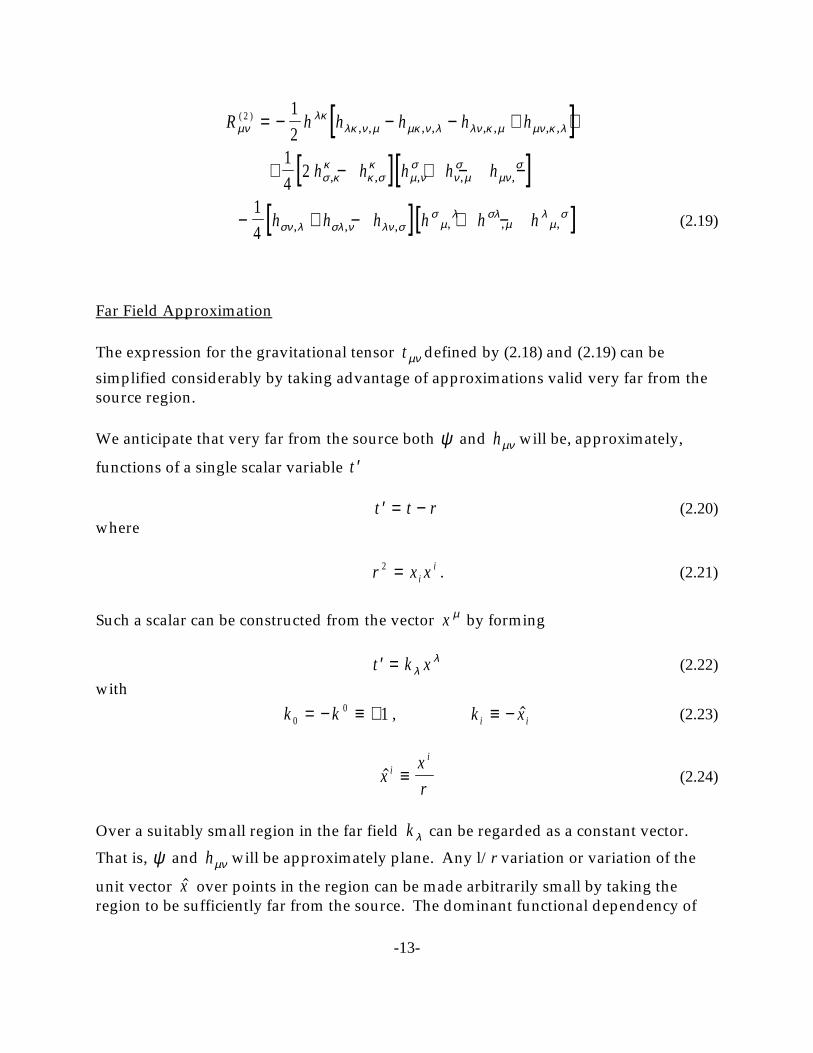
-13-

[ ]R h h h h hµνλκ

λκ ν µ µκ ν λ λν κ µ µν κ λ( )2 1

2= − − − + +, , , , , , , ,

[ ][ ]+ − + − −1

42 h h h h hσ κ

κκ σκ

µ νσ

ν µσ

µνσ

, , , , ,

(2.19)[ ][ ]− + − + −1

4h h h h h hσν λ σλ ν λν σ

σµ

λ σλµ

λµ

σ, , , , , ,

Far Field Approximation

The expression for the gravitational tensor defined by (2.18) and (2.19) can bet µν

simplified considerably by taking advantage of approximations valid very far from thesource region.

We anticipate that very far from the source both and will be, approximately,ψ hµν

functions of a single scalar variable ′t

(2.20)′ = −t t rwhere

. (2.21)r x xii2 =

Such a scalar can be constructed from the vector by formingx µ

(2.22)′ =t k xλλ

with

, (2.23)k k00 1= − ≡ + k xi i≡ −

(2.24)xx

ri

i

≡

Over a suitably small region in the far field can be regarded as a constant vector. k λ

That is, and will be approximately plane. Any l/r variation or variation of theψ hµν

unit vector over points in the region can be made arbitrarily small by taking thexregion to be sufficiently far from the source. The dominant functional dependency of

-14-

our solutions will be on the scalar . This fact can be exhibited explicitly by′ = −t t rexpressing all partials of and asψ hµν

(2.25)ht

x

dh

d tk h k hµν σ σ

µνλ σ

λµν σ µν

∂∂

δ, =′

′= =

and(2.26)ψ ψσ σ,

= k

where

, (2.27)( ) ( )h h k x h tµν µν λλ

µν= = ′

, (2.28)( ) ( )ψ ψ ψλλ= = ′k x t

, (2.29)( ) ( )f t

d f t

d t≡

. (2.30)∂∂

δλ

σ σλx

x=

Again, because outside the source region,Tµν = 0

and (2.31)*2 0hµν = *

2 0ψ =

in the far field. If (2.25) is used in the first of these, we find

,( )*2h h k h k k hµν µν ρ

ρρ µν

ρρ

ρµν= = =, , ,

implying that

. (2.32)k kρρ = 0

Obviously the same condition follows from the second of (2.31).

We may now use (2.25) and (2.26) to express the coordinate condition (2.13) in the farfield. From (2.13) we have

-15-

. (2.33)k h k hλλ

µ µλ

λϕ ψ = +

−0

1 1

2

Since any constant of integration is of no consequence in the radiation of energy, (2.33)can be integrated or differentiated by inspection. In particular

(2.34)k h k hλλ

µ µλ

λϕ ψ= +

−0

1 1

2and

. (2.35)k h k hλλ

µ µλ

λϕ ψ = +

−0

1 1

2

These relations stemming from the coordinate condition can be used to effect a

simplification of (2.19). First, we notice that the first factor of the second term ofRµν( )2

(2.19) is just the coordinate condition itself,

.2 2 01h h kσ κ

κκ σκ

σϕ ψ, ,− = −

For the rest of (2.19), the objective is to use (2.33), (2.34) and (2.35) to draw out of eachterm explicit dependency on . For example,k kµ ν

h h h k k h k k h hλκµν κ λ

λκκ λ µν

κκ

λλ µνϕ ψ, , = = +

=−

01 1

20

nn

from (2.32), and pp

h h k h k h k k hλν σσ

µλ

σ λνλ σ

µ µ νλ

λϕ ψ, , = = +

− 0

1

21

2nn

To ease the notation let

. (2.36)z h≡ +−ϕ ψ λλ0

1 1

2

Then (2.33), (2.34), and (2.35) imply that

(2.37)R k k z z h h z h h zµν µ νλκ

λκ λκλκϕ ψ( )

2

01 21

2

1

4

1

2= − + − +

−

-16-

in the far field.

and can be related to each other in the following way. From the scalar fieldh λλ ψ

equation (2.9) we have

, (2.38)( ) ( )ψ

ωλλ

& &

& & &

& &x t d xT x t x x

x x,

,= −

+′

′ − ′ −′ −∫2

3 23

and from the tensor field equation (2.14) we have

( ) ( )h x t d x

T x t x x

x xµνµνϕ& &

& & &

& &,,

= ′′ − ′ −

′ −−

− ∫4 01 3

. (2.39)( )

−++

′′ − ′ −

′ −

∫η

ωωµν

λλ1

3 23d x

T x t x x

x x&

& & &

& &,

Contraction of (2.39) gives

. (2.40)( ) ( )h x t d x

T x t x x

x xλλ λ

λ

ϕωω

& && & &

& &,,

= −++

′′ − ′ −

′ −− ∫4

1 2

3 201 3

By comparing (2.38) and (2.40) we find immediately that

, (2.41)( ) ( ) ( )h x t x tλλ ϕ ω ψ& &

, ,= +−2 1 201

and when this is used in the three terms of (2.37), which involve , we find thatz

.( ) ( ) ( )[ ]R k k h h h hµν µ νλκ

λκλκ

λκ ω ϕ ω ψψ ω ψ( ) 20

2 21

2

1

22 1 2 1 2= − +

+ + + + +

−

(2.42)The second term of the definition (2.18) of involvest µν

[ ] [ ]η ηλρλρ

λρλ ρ

ρρR k k k k( )2 0= = =

by (2.32). Therefore, from (2.18) and (2.42), the energy-momentum tensor associatedwith the tensor part of the gravitational field is

-17-

(2.43)

( ) ( ) ( )[ ]t

k k h h h hµν

µ νλκ

λκλκ

λκ

πϕ

ω ϕ ω ψψ ω ψ=

− +

+

+ + + + +

−8

1

2

1

2

2 1 2 1 2

0

01 2

Averaging of the Field

Thus far we have incorporated approximations valid for a weak field far from thesource, but have not sacrificed temporal detail. We could, if we wished, compute theinstantaneous with (2.43) as a basis. However, such an attempt would bedE d textraordinarily complex and would not be useful. The overall effect on a system, suchas a binary, is better characterized by the average flux of energy away from the system.

Suppose that the (or ) waves have a discrete spectra1 representation. It is clearhµν ψthen that the longest periodicity T that can be seen temporally will be proportional tothe inverse of the difference of the closest pair of frequency components in the wave. Therefore, it would be appropriate to evaluate the average of over an intervaldE d tequal to or greater than T. It turns out that the loss of temporal detail introduced bysuch averaging will simplify our final results strikingly.

A large class of problems, of which the binary system is an example, have discretespectral representations so that the averaging process just described is applicable. Other problems, such as the collision of particles to be considered later, are not periodicbut are represented by continuous spectra. In these cases the "longest periodicity"becomes infinitely long and averaging no longer has a practical meaning. But it ispossible to define the power spectral density associated with the wave in such cases andwe will find that this too will result in a considerable simplification of final results.

The instantaneous flux of energy through a surface of area in the direction isr d2 Ω x

(2.44)dE

dtr d x ti i= 2 0Ω

and the average flux is

. (2.45)dE

dtr d x ti i= 2 0Ω

Consider, in particular, the average of the first term of (2.43), which involves

-18-

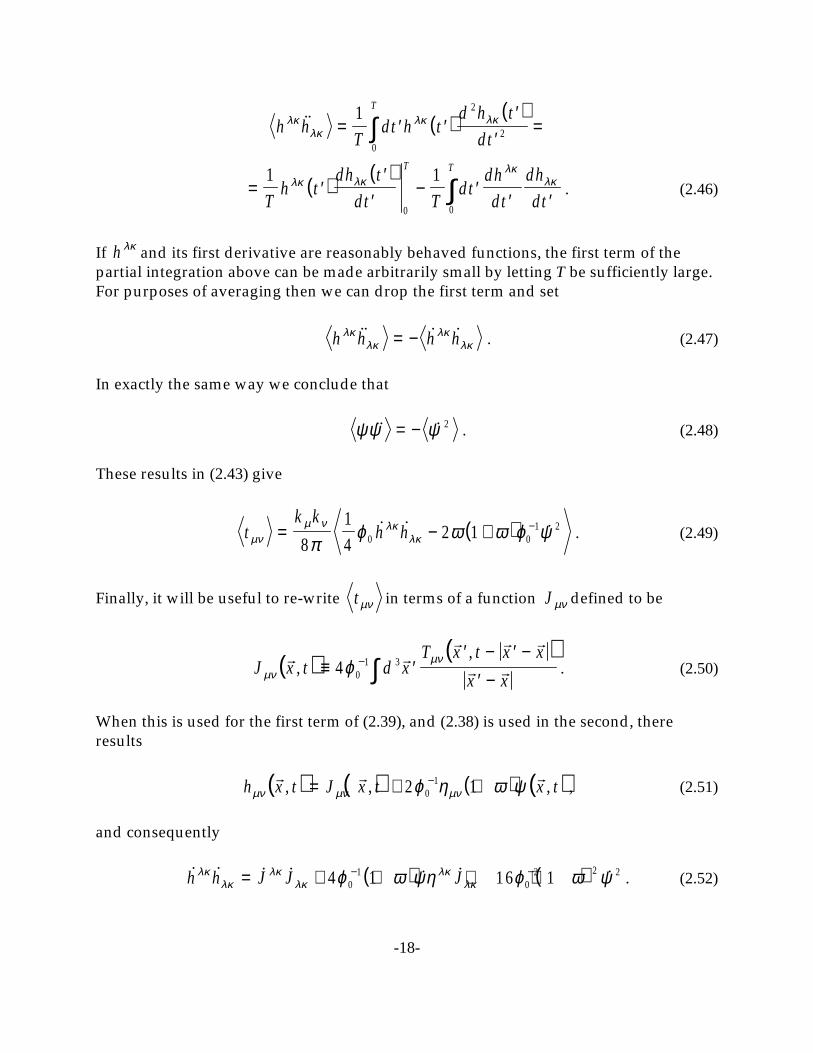
( ) ( )h h

Tdt h t

d h t

d t

Tλκ

λκλκ λκ = ′ ′

′′

=∫1

0

2

2

. (2.46)( ) ( )= ′

′′

− ′′ ′∫

1 1

0 0Th t

dh t

d t Td t

dh

d t

dh

dt

T Tλκ λκ

λκλκ

If and its first derivative are reasonably behaved functions, the first term of theh λκ

partial integration above can be made arbitrarily small by letting T be sufficiently large. For purposes of averaging then we can drop the first term and set

. (2.47)h h h hλκλκ

λκλκ

= −

In exactly the same way we conclude that

. (2.48)ψψ ψ = − 2

These results in (2.43) give

. (2.49)( )tk k

h hµνµ ν λκ

λκπϕ ω ω ϕ ψ= − + −

8

1

42 10 0

1 2

Finally, it will be useful to re-write in terms of a function defined to bet µν J µν

. (2.50)( ) ( )J x t d x

T x t x x

x xµνµνϕ& &

& & &

& &,,

≡ ′′ − ′ −

′ −− ∫4 0

1 3

When this is used for the first term of (2.39), and (2.38) is used in the second, thereresults

, (2.51)( ) ( ) ( ) ( )h x t J x t x tµν µν µνϕ η ω ψ& & &, , ,= + +−2 10

1

and consequently

. (2.52)( ) ( ) h h J J Jλκλκ

λκλκ

λκλκϕ ω ψη ϕ ω ψ= + + + +− −4 1 16 10

10

2 2 2

-19-

By contracting (2.50), and comparing with (2.38), we find

, (2.53)( )η ϕ ω ψλκλκ

λλJ J= = − +−2 3 20

1

and consequently that

. (2.54)( )η ϕ ω ψλκλκ

λλ J J= = − +−2 3 20

1

This last result may be used to eliminate from (2.52) and (2.49) to giveψ

, (2.55)( )tk k

GJ J Jµν

µ ν λκλκ

λλπ

ωω

ωω

=+

+−

++

8

2

3 2

1

2

1

3 2

22

where we have used also (2.16) for .ϕ0

Conservation Law and Moments

Analysis of the radiation in terms of multipoles is a result of one further approximation: the expansion of in a Taylor series about . That is,J µν ′ = −t t r

( ) ( ) ( )J x t

rd x T x t x d x x

T x t

tµν µν

µν

ϕ∂

∂& & & & &

&

, , ,

= ′ ′ ′ + ⋅ ′ ′′ ′

′+

− ∫∫4

10

1 3 3

, (2.56)( ) ( )+ ′ ⋅ ′

′ ′′

+

∫

1

23 2

2

2d x x xT x t

t& &

&

,∂

∂

µν

where we have used

and & &′ − ≅−x x r1 1

& & &′ − ≅ − ⋅ ′x x r x x

for .r x>> ′&

Let us define the following moments of the mass-energy distribution:

-20-

, (2.57)( ) ( )M t d x T x t≡ ∫ 3 00& &,

, (2.58)( ) ( )D t d x x T x tk k≡ ∫ 3 00& &,

. (2.59)( ) ( )Q t d x x x T x tij i j≡ ∫ 3 00& &,

The conservation law (2.3) becomes, in the weak field limit,

(2.60)T µνν, = 0

and implies the relations [See Appendix A]

(2.61)( ) ( ) ( )d x T x tt

d x x x T x t Q tjk j k jk32

23 001

2

1

2& & & &

, , = =∫∫∂∂

(2.62)( ) ( ) ( )d x T x tt

d x x T x t D tk k k3 0 3 00& & & &∫ ∫= =, , ∂∂

. (2.63)( ) ( ) ( )∂∂t

d x x T x t d x T x t Q tk j jk jk3 0 3 1

2∫ ∫= =& & & &, ,

We use the expansion (2.56) of to write , , and in terms of the momentsJ µν J 00 J i0 J ij

(2.57) - (2.59).

First, from (2.56) we have

( ) ( ) ( )J x tr

d x T x t xt

d x x T x tii00

01 3 00 3 004

1& & & & &, , ,= ′ ′ ′ +

′′ ′ ′ ′

+− ∫ ∫ϕ

∂∂

. (2.64)( )+′

′ ′ ′ ′ ′ +

∫1

2

2

23 00

,x xt

d x x x T x ti ji j∂

∂& &

From the definitions of the moments and the relations implied by the conservation law,

we have for , out to second moments,J 00

-21-

. (2.65)( ) ( ) ( ) ( )J x tr

M t x D t x x Q tii

i jij00

014

1 1

2*

, = ′ + ′ + ′

−ϕ

For we need only two terms of the expansion (2.56) in order to include moments toJ i0

the second.

. (2.66)( ) ( ) ( )J x tr

d x T x t xt

d x x T x ti ik

k i00

1 3 0 3 041& & & & &

, , ,= ′ ′ ′ +′

′ ′ ′ ′

− ∫ ∫ϕ∂

∂

Relations (2.62) and (2.63) then give

. (2.67)( ) ( ) ( )J x tr

D t x Q ti ik

ik00

141 1

2&

, = ′ + ′

−ϕ

And for only one term of (2.56) is required, giving immediatelyJ ij

. (2.68)( ) ( )J x tr

Q tij ij&, = ′−2

10

1ϕ

The conservation law also implies that [See Appendix A]

and . (2.69)M = 0 D k = 0

Therefore, from (2.65), (2.67), and (2.68) we have

(2.70) Jr

x x Qi jij00

012

1= −ϕ

(2.71) Jr

x Qik

ik00

121

= −ϕ

. (2.72) Jr

Qij ij= −21

01ϕ

To evaluate (2.55), we require , which may be written J Jλκλκ

-22-

. (2.73) J J J J J J J Jii

ijij

λκλκ = + +00

000

02

The signs of and are independent of the raising/lowering of the pair of indices,J 00 J ij

but

. (2.74)J J Ji ii

0 00= = −η ηα β

αβ

When this and (2.70) - (2.72) are used in (2.73) we get

. (2.75)( ) ( )( ) ( ) J Jr

x x Q x Q x Q Q Qi jij

kik

jij ij

ijλκ

λκ ϕ= − +

−41

202

2

2

In completely analogous manner, we find

, (2.76) J J J J Jii

ii

λλ = + = − +0

000

so that from (2.70) - (2.72) we get

, (2.77)( ) Jr

x x Q Qi jij k

kλ

λ ϕ= − −−21

01

and finally

. (2.78)( ) ( ) ( ) ( ) Jr

x x Q Q x x Q Qi jij k

k i jij k

kλ

λ ϕ2

02

2

2 24

12= − +

−

When (2.75) and (2.78) are put into (2.55), and (2.16) is used again to eliminate , weϕ0

find

( ) ( )tk k G

rx x Qi j

ijµν

µ ν

πω

ωω ω

ω=

++

+ ++

−8

3 2

2

2 8 7

2 3 22

2

2

2

. (2.79)( )( ) ( ) ( )− + +++

− x Q x Q Q Q Q x x Q Qk

ikj

ij ijij

kk i j

ij kk

1

2

1

3 22

2ωω

-23-

Total Power

We now use (2.79) for in (2.45) and integrate over all directions in order tot µν

compute the total average flux of energy due to the tensor wave,

. (2.80)dE

dtr d x ti i

to tal(te n sor)

= ∫2 0Ω

Note that

,[ ] ( )( )[ ] [ ] x t x k k x xi i i i i i0 0 1= = − − =

which simplifies the evaluation of (2.80). Integration over all directions is accomplishedreadily with the help of

(2.81)d x xi j ijΩ =∫4

3

πδ

and

. (2.82)( )d x x x xi j l m ij lm il jm im jlΩ ∫ = + +4

15

πδ δ δ δ δ δ

The result is:

( )( ) ( )( )dE

d t

GQ ij

to ta l(te n so r)

=+ +

+ + −60

1

3 2 224 76 592 2

ω ωω ω

(2.83)( )( )− + +8 12 32 2ω ω Q k

k

We have already noted that the Brans-Dicke theory goes over to general relativity when. In this limit, (2.83) becomesω → ∞

, (2 .84)( ) ( )dE

dt

GQ Qij k

kto ta lG R

= −15

32 2

which is recognized as the result familiar from general relativity (14). It is customary todefine the traceless tensor

-24-

(2.85)D Q Qij ij ij kk≡ −3 δ

in terms of which (2.84) becomes

. (2.86)( )dE

dt

GD ij

to talG R

=45

2

Unfortunately, a comparable simplification does not follow if (2.85) is used in the resultfor the Brans-Dicke theory (2.83).

Energy-Momentum of the Gravitational Field - Scalar Part

To complete the analysis in the Brans-Dicke theory, we must carry through theanalogous steps for the flux of energy carried by the scalar field. The weak fieldapproximation of the tensor associated with the scalar field is found by applyingT( )ϕ µν

(2.5) and (2.26) to (2.4). This gives

T k k k k( ) ϕ µν µ ν µν ρ

ρωπ

ϕ ψ η ψ= −

+−

8

1

201 2 2

. (2.87)( )+ −1

8πψ η ψµ ν µν ρ

ρk k k k

The second and fourth terms above drop out in the far field due to (2.32) leaving

. (2.88)( )Tk k

( ) ϕ µν

µ ν

πωϕ ψ ψ= +−

8 01 2

Recalling that is small, one might be inclined to ignore the first term of (2.88) in favorψof the second. However, consideration of the averaging process which is to be applied,as for the tensor field, reveals that it is the second, rather than the first, term which isappropriately ignored.

Consider

.ψψ ψ

= ′′

=′∫

1 12

20 0T

dtd

d t T

d

dt

T T

-25-

If is a reasonably behaved function, becomes arbitrarily small as T isd dtψ ′ ψincreased. On the other hand,

ψψ2

0

21

= ′′

∫T

dtd

d t

T

approaches a meaningful average as T is increased because of the positive definiteperiodic kernel. Therefore, for purposes of averaging, it is the first term of (2.88) that isto be retained.

. (2.89)Tk k

( )ϕ µν

µ ν

πωϕ ψ= −

8 01 2

Using (2.54) for , we find thatψ

. (2.90)( ) ( )Tk k

J( )

φ µνµ ν λ

λπωϕ

ω=

+8

1

3 20 2

2

Finally, we use (2.78) for and (2.16) for to get( )J λλ

2ϕ0

( )( ) ( )Tk k G

rx x Qi j

ij( ) ϕ µν

µ ν

πω

ω ω=

+ +−

16 3 2 22

2

. (2.91)( ) ( )− +22

Q x x Q Qkk i j

ij kk

Note that the contribution from the scalar field goes to zero, as it should, as we makethe transition to general relativity by letting go to infinity.ω

When is substituted for in (2.45) and then integrated over all directions, weT( )ϕ µν t µν

find, with the help of (2.81) and (2.82), that

. (2.92)( )( ) ( ) ( )dE

dt

GQ Qij k

kto ta l

(scala r)

=+ +

+10 3 2 2

1

32 2ω

ω ω

The grand total flux due to both scalar and tensor quadrupole radiation is given by thesum of (2.83) and (2.92):

-26-

( )( ) ( )( )dE

dt

GQ ij

to ta l

=+ +

+ + −60

1

3 2 224 78 592 2

ω ωω ω

. (2.93)( )( )− + +8 6 32 2ω ω Q k

k

Application to a Binary System

In order to evaluate expressions for the flux such as (2.83), (2.92), or (2.93) it is necessaryto form explicit expressions for

Q Qijij

and

( )Q kk

2

for the system under consideration. For a binary system, we shall assume that in thefirst approximation the motion is Keplerian. Therefore averaging will be over oneorbital period. We will first compute the averages that apply to a single body of thepair. It is then a simple matter of scaling to adapt the results to the system of twobodies.

For a point mass m, defined by (2.59) is( )Q tij

( ) ( )Q t d x x x T x tij i j≡ =∫ 3 00& &,

(2.94)( )( ) ( )( ) ( )( )= − − −∫∫∫ d x d x d x m x x x x t x x t x x ti j1 2 3 1 1 2 2 3 3δ δ δ

where is the integration variable and is the position of the mass. In terms of thex xspecific system PSR 1913+16, we shall define

mass of pulsar,m =mass of companion, and (2.95)M =

.( )µ =+

G M

M m

3

2

will be used to account for the fact that may not be small when compared with .µ m M

-27-

Since the orbit is Keplerian and, hence, planar, we can pick the coordinate system so

that is zero. Then (2.94) reduces tox 3

(for i or j = 3) (2.96)( )Q tij = 0

(2.97)( ) ( )( ) ( ) ( )( )Q t m x t Q t m x t11 1 2 22 2 2= =,

. (2.98)( ) ( ) ( ) ( )Q t Q t m x t x t12 21 1 2= =

As is well known, the position in the orbit plane is a transcendental function of the time. We shall, therefore, work with the parametric representation of the motion (15)

( ) ( )r a E ta

E E= − = −13

εµ

εcos , sin

(2.99)

( ) ( ) ( ) ( )x E a E x E a E1 2 2 1 21= − = −cos , sinε ε

where = orbital radius to , = semimajor axis of the orbit of , = eccentricity,r m a m ε= eccentric anomaly. Over one orbit, ranges from 0 to . Since , rather thanE E 2π E

, will be used to locate the body in its orbit, we must re-write the expression for thettime-average of a function so that it involves integration on .dE

. (2.100)( )fT

d t f tT

≡ ∫1

0

For a Keplerian orbit has the valueT

. (2.101)Ta

= 23

πµ

From (2.99) and (2.101) we have

-28-

,( )tT

E E= −2π

ε sin

(2.102)

.( )dtT

E dE= −2

1π

ε cos

Therefore, if , we may write (2.100) as( ) ( )( )f t g E t=

. (2.103)( ) ( )( )f t g E E dE= −∫1

21

0

2

πε

π

cos

Accordingly, we will first express the required contractions of in terms of theQ ij

eccentric anomaly and will then use (2.103) to compute the time average over oneorbital period.

Note incidentally that in what follows we can raise/lower all space indices without

regard for sign changes because .η δi j i j=

( )Q kk

2

From (2.97) and (2.99) we can write

( ) ( )[ ]Q Q Q m x x m rkk = + = + =1

12

21 2 2 2 2

or

. (2.104)( ) ( )Q E m a Ekk = −2 21 ε cos

Using (2.102), we find that all time derivatives are equivalently

. (2.105)( )d

dt

dE

dt

d

dE TE

d

dE= = − −2

1 1πε cos

We find, therefore, that the derivatives of areQ kk

-29-

, sinQ m aT

Ekk =

2

22επ

,( ) cos cosQ m aT

E Ekk =

− −2

212

21ε

πε

( )

sin

cosQ m a

T

E

Ek

k = −

−

=22

12

3

3επ

ε

, (2.106)( )= −−

21

3 2

5 2 3ma

E

Eε

µεsin

cos

from which

. (2.107)( ) ( )

sin

cosQ m

a

E

Ek

k2 2 2

3

5

2

641

=−

εµ

ε

From (2.103) we find that

(2.108)( ) ( )

sin

cosQ m

a

E

EdEk

k2 2 2

3

5

2

50

4

1=

−∫πε

µε

π

where we have used also the symmetry of the integrand over the range of integration.

In Appendix B we show that

, (2.109)( ) ( )sin

cos

2

5

2

2 7 20 1 8

4

1

E

EdE

−=

+−∫ ε

π εε

π

so that we have finally from (2.108) that

. (2.110)( ) ( )( )

Q ma

kk

2 23

5

2 2

2 7 2

1

2

4

1=

+−

µ ε εε

-30-

Q Qijij

From the properties (2.96) - (2.98) of we can writeQ ij

. (2.111)( ) ( ) ( ) Q Q Q Q Qijij = + +11 2 12 2 22 2

2

We take each of the terms in order. First, from (2.97) and (2.99) we have that

. (2.112)( ) ( )Q E m a E11 2 2= −cos ε

Using (2.105) to compute the various derivatives we find

,( )

sin cos

cosQ m a

T

E E

E11 22

2

1= −

−−

π εε

,( ) ( ) cos cos cos cosQ m aT

E E E E11 2

23 2 3 22

21 2 1= −

− − − + −−π

ε ε ε ε

and

( ) ( cos sin cosQ m aT

E E E11 2

35 22

21= −

− +−π

ε ε

. (2.113))+ − − +2 4 3 42 3ε ε εcos cosE E

Likewise, from (2.97) and (2.99) we have

, (2.114)( ) ( )Q E m a E22 2 2 21= − ε sin

which leads to the derivatives

,( )( ) cos sin cosQ m aT

E E E22 2 2 122

1 1=

− − −π

ε ε

,( )( ) ( ) cos cos sin cosQ m a

TE E E E22 2

22 3 2 2 32

21 1=

− − − −−π

ε ε ε

-31-

.( )( ) ( ) cos sin cos cosQ m aT

E E E E22 2

3

2 5 222

1 1 3 4=

− − − +−π

ε ε ε ε

(2.115)

And finally, from (2.98) and (2.99) we have

, (2.116)( ) ( )Q Q m a E E12 21 2 2 1 21= = − −ε εsin cos

which leads to the derivatives

,( ) ( ) ( ) cos cos cosQ m aT

E E E12 2 2 1 2 1 221 1 2 1=

− − − −−π

ε ε ε

,( ) ( ) ( ) cos sin cos cosQ m aT

E E E E12 2

2

2 1 2 3 221 1 2 4 2=

− − − +−π

ε ε ε ε

( ) ( ) ( cos cosQ m aT

E E12 2

3

2 1 2 5 2 222

1 1=

− − +−π

ε ε ε

. (2.117))+ + − − +3 3 4 23 2 2ε ε εcos cos cosE E E

When results (2.113), (2.115), and (2.117), together with (2.101) for , are used inT(2.111), one finds after considerable algebra that

. (2.118)( ) ( )[ ] cos sinQ Q ma

E Eijij = − − +−4 1 8 12

3

56 2 2 2µ

ε ε ε

On substitution of (2.118) into (2.103) for the average there results

. (2.119)( )

( )

sin

cosQ Q m

a

E

EdEij

ij =− +

−∫4 8 1

12

3

5

2 2 2

50π

µ ε εε

π

5 Ref. (16), entry 3.661 4 with , , , and .a = 1 b = −ε n = 4 a b>

-32-

Note that the second term of the above is identically (2.108), which has the value givenby (2.110). The first term is evaluated using5

( ) ( )dE

EP

1 1

1

15 2 5 2

04 2−

=− −

∫ ε

πε ε

π

cos

,( ) ( )P x x x44 21

835 30 3= − +

which leads to

. (2.120)( ) ( )dE

E1 8

3 24 8

15

4 2

2 9 20 −

=+ +−∫ ε

π ε εε

π

cos

Consequently, the first term of (2.119) is

,( )43 24 8

12

3

5

4 2

2 7 2ma

µ ε εε

+ +−

and the complete evaluation of (2.119) using also (2.110) is

. (2.121)( ) Q Q m

aij

ij =+ +−

1

2

25 196 64

12

3

5

4 2

2 7 2

µ ε εε

Scaling

Results (2.110) and (2.121) apply to the motion of one body in a Keplerian orbit aboutma second body . If used as is in the radiation formula (2.93) they will account for theMenergy loss due to the motion of , but not of . The overall loss rate due to them Mmotion of both bodies is found from a simple scaling argument.

Let subscript 1 denote the pulsar and 2 the companion and, as above, let them Morigin of coordinates be at the barycenter. This condition is defined by

-33-

m x M xi i1 2 0+ =

or,

. (2.122)xm

Mxi i

2 1= −

The overall moment for the system consisting of both and isQ ij m M

, (2.123)( )Q m x x M x xm

Mm M x xij i j i j i j= + = +1 1 2 2 1 1

where we have used (2.122) to express the moment in terms of the motion of . Thismdiffers from (2.97) and (2.98) only by the factor of . Therefore, results( )m M M+(2.110) and (2.121) can be made to apply to the system of two bodies of masses andm

by simply scaling by the factor . When this is done, and theM ( )( )m M M+2

definition (2.95) of is introduced, we have for the binary systemµ

(2.124)( ) ( )( )( )

QG m M

a m Mk

k2

3 2 7

5 4

2 2

2 7 22

4

1=

++−

ε εε

and,

. (2.125)( ) ( ) Q Q

G m M

a m Mij

ij =+

+ +−

3 2 7

5 4

4 2

2 7 22

25 196 64

1

ε εε

For the special case of general relativity, these two results in (2.84) give

. (2.126)( ) ( )dE

dt

G m M

a m Mto ta lG R

=+

+ +

−

32

5

1

1

4 2 7

5 4

2 4

2 7 2

7324

3796ε ε

ε

-34-

Effect on Orbital Period

One does not measure directly but rather the change of orbital period induceddE d t T

by . Therefore, in order to apply our results to observation we need as a finaldE d tstep to relate to .dE d t dT d t

The semimajor axis of the relative orbit is

′ =+

am M

Ma

where it is to be recalled that is the semimajor axis of the pulsar orbit. The totalaenergy of a Keplerian binary system isE

(2.127)( )EG m M

a

G m M

a m M= −

′= −

+2 2

2

from which

. (2.128)( )aG m M

m ME= −

+−

21

2

The orbital period can be related to the energy by combining (2.101), (2.95) forT Eand (2.128). The result isµ

. (2.129)( ) ( )T Gm M

m ME=

+

− −π

3 3 1 2

3 2

2

By taking the time derivative and afterward re-introducing (2.127) to restore theparameter , we find that a

. (2.130)( )dT

dtT

m M

m

a

G M

dE

dt= =

+ 6

2 5

3 7π

-35-

Numerical Results for PSR 1913+16

We now use the published numerical values for the specific example of PSR 1913+16 tocompute values for (2.124) and (2.125). These will be used in (2.93) to evaluate

from which can be estimated using (2.130).dE dt dT d t

We take the following approximate values from Taylor et al. (1) for PSR 1913+16:

1.39 2.765 x 1033 gm = M s u n =1.44 2.864 x 1033 gM = M s u n =

0.81sin i = 2.3424 light-sec = 7.0225 x 1010 cma isin =

8.67 x 1010 cma = 0.617155ε =

Also we use: 6.673 x 10-8 dyn cm2 g-2 G =

2.998 x 1010 cm sec-1c =

Note that for dimensional reasons we have to restore a factor of to the denominatorc5

of (2.93).dE d t

First, we find from (2.130) that for PSR 1913+16

2.2061 x 10-44 . (2.131)T =se c

g cm

3

2

dE

dtFrom (2.124) and (2.125) we get

3.26 x 1090 (2.132)( )Q kk

2=

g cmse c

2

3

2

and

2.78 x 1092 . (2.133) Q Qijij =

g cmse c

2

3

2

The average total radiation rate for the binary system in the Brans-Dicke theory is foundfrom (2.93) and the above to be

-36-

Figure 1. Orbital decay rate for PSR 1913+16 in the Brans-Dicke theory.

. (2.134)( )( )dE

dt=

+ ++ +

3 .0 5 x 1 0 9 .9 4 x 1 0 7 .5 3 x 1 0 g cmse c

32 3 2 3 2 2

3

ω ωω ω

2

3 2 2

When this is used in (2.131) for the effect on the orbital period, we find

, (2.135)( )( )T =

+ ++

6 .7 3 x 1 0 2 .1 9 x 1 0 1 .6 6 x 1 03 + 2

se cse c

-12 -11 -11ω ωω ω

2

2

where a positive result indicates a decreasing orbital period. In the limit , thisω → ∞goes over to the general relativistic prediction

3.36 x 10-12 . (Gen. Rel.) (2.136)T =se cse c

Figure l is a plot of from (2.135) for PSR 1913+16 as a function of the free parameterT

. Also indicated are the observational limits on set by Taylor et al., and the limitingω T

-37-

general relativistic value (2.136). It is clear that the prediction for all positive values ofis comfortably within the observational limits. Consequently, it is not possible toω

validate the Brans-Dicke theory or to establish bounds on from current observationsωof the orbital decay rate of PSR 1913+16 under the assumption of gravitational radiationin the quadrupole mode.

3.0 Gravitational Radiation from Colliding Bodies in Brans-Dicke Theory

General Results

We turn now to the problem of computing the gravitational radiation associated with asystem of bodies in collision in the weak field limit of the Brans-Dicke theory. Theresults will be useful as a basis for studying other systems such as a hot gas in thermalequilibrium.

Spectral Representation of the Fields

Since the motion of the system is not periodic, the averaging technique that we appliedin the previous section cannot be utilized. We assume, as before, that very far from thesource and are functions of the scalar ψ hµν ′t

(3.1)′ = − =t t r k xλλ

(3.2)k k k xi i00 1= − = + = −,

(these as before). (3.3)xx

ri

i

≡

We assume further that in the far field can be represented by a continuous spectralhµν

distribution such thateµν

(3.4)( ) ( ) ( )h x t d e x i k xµν µν λλϖ ϖ ϖ& &

, , exp=−∞

+∞

∫which implies that

-38-

. (3.5)( ) ( ) ( )e x d t h x t i tµν µνϖπ

ϖ& &, , exp= ′ ′ − ′

−∞

+∞

∫1

2

We use the symbol for the frequency in order to distinguish it from the freeϖparameter of the Brans-Dicke theory, and the spatial angular measure .ω dΩ

The linearity of the field equations, (2.9) and (2.14), in the weak field limit assures usthat we can represent the scalar field also by a continuous distribution of the same formas for . That ishµν

(3.6)( ) ( ) ( )ψ ϖ ϖ ϖ λλ& &

x t d a x i k x, , exp=−∞

+∞

∫and

. (3.7)( ) ( ) ( )a x d t x t i t& &

, , expϖπ

ψ ϖ= ′ ′ − ′−∞

+∞

∫1

2

Though now in the form of integrals over continuous distributions, and still haveψ hµν

the functional dependency on assumed in expressions (2.43) and (2.88) for and′t t µν

. Keeping (3.1) in mind, we can immediately express both tensors using (3.4) andT( )ϕ µν

(3.6). We find from (2.43) that

( )[ ] ( ) ( )tk k

d d e x e xµνµ ν λκ

λκπϖ ϖ ϕ ϖ ϖϖ ϖ ϖ= ′ ′ + ′ −∫∫

−∞

+∞

812 0

2 12

& &, ,

( ) ( )( ) ( )[ ] ( ) ( )− + + ′ + + ′ ′ ×−2 1 2 1 201 2ω ϕ ω ϖ ω ϖϖ ϖ ϖa x a x

& &, ,

(3.8)( )( )× + ′exp i k xϖ ϖ λλ

and from (2.88) that

( ) ( ) ( )( )Tk k

d d a x a x i k x( ) , , expϕ µνµ ν

λλ

πω ϕ ϖ ϖ ϖ ϖ ϖ ϖ= −

′ ′ + ′ +−

−∞

+∞

∫∫8 01 & &

-39-

. (3.9)( ) ( )+

−∞

+∞

∫ d a x i k xϖ ϖ ϖ ϖ λλ2 &

, exp

Definition of the 2-sided Power Spectral Density Function

Because the distributions and are continuous in , there are( )e xµν ϖ&, ( )a x

*,ϖ ϖ

components of each that are arbitrarily close together in frequency. As a consequence,the longest periodicity, which determines the minimum averaging interval , tends toTinfinity. Therefore, the averaging process that we used previously no longer has apractical meaning, but it is still defined in the mathematical sense.

If we were to carry out the (mathematical) averaging process, we would have tointegrate the instantaneous over all time giving , the total energy emitted bydE d t E

the system. Since and are now related to and by transform pairψ hµν a eµν

relationships, (3.6), (3.7), and (3.4), (3.5), we should be able to define a new functionthat, when integrated over all frequency, also gives the total energy . That is,( )P ϖ E

. (3.10)( )E d P=−∞

+∞

∫ ϖ ϖ

Of the infinity of functions that satisfy (3.10), the most natural choice follows, not( )P ϖsurprisingly, from an attempt to integrate over all time as would be required bydE d tthe averaging process.

Consider first (2.44) for in the tensor field. Integration over all time gives, for adE d tparticular direction ,x

. (3.11)( )dE r d x d t t ti i= ′ ′−∞

+∞

∫2 0Ω

( appears on the left side because we have not yet integrated over all directions .dE xOtherwise should be considered on the same footing as in (3.10) for purposes ofdE Edefining the power spectral density). Clearly, integration of over all time is ant µν

essential step in our computation of the total energy radiated by a system.

-40-

Recalling (3.1), we see from (3.8) that integration of over all time involvest µν

. (3.12)( )( ) ( )d t i t′ + ′ ′ = + ′−∞

+∞

∫ exp ϖ ϖ πδ ϖ ϖ2

Therefore, one of the frequency integrals from (3.8), say that on , can be performed′ϖimmediately, with the result that

(3.13)′ = −ϖ ϖ

in the remaining integral. Inspection of (3.5) and (3.7) reveals thatϖ

(3.14)( ) ( )e x e xµν µνϖ ϖ& &, ,− = ∗

and

, (3.15)( ) ( )a x a x& &

, ,− = ∗ϖ ϖ

assuming and to be real fields, and "star" denotes complex conjugate. We have,hµν ψconsequently, that

( )dt t t′ ′ =−∞

+∞

∫ µν

. (3.16)( ) ( ) ( ) ( )k kd e x e x a x

µ ν λκλκϖ ϕ ϖ ϖ ω ω ϕ ϖ ϖ

4

1

42 10 0

1 2 2& & &, , ,∗ −

−∞

+∞

− +

∫

An analogous argument holds for the scalar field with substituted for inT( )ϕ µν t µν

(3.11), but there is a minor difference introduced by the fact that the second term of(3.9) involves only a single integral. Integration of over all time involves, fromT( )ϕ µν

the second term of (3.9),

( ) ( )d a x d t i tϖ ϖ ϖ ϖ2 &, exp

−∞

+∞

−∞

+∞

∫ ∫ ′ ′ =

. (3.17)( ) ( )= =−∞

+∞

∫2 02π ϖ ϖ ϖ δ ϖd a x&

,

-41-

It is noteworthy that in the averaging process used in the previous section it was alsothis term that dropped out. We have finally from (3.9) that

. (3.18)( ) ( )d t T tk k

d a x′ ′ =−∞

+∞−

−∞

+∞

∫ ∫( ) ,ϕ µνµ ν ω ϕ ϖ ϖ ϖ4 0

1 2 2&

With (3.16) or (3.18) substituted into (3.11) for the respective field, we see that we nowhave expressions for the total energy that are of the form of (3.10). Using to( )dP ϖindicate that we have not yet integrated over all directions, we identify by comparisonwith (3.10) that for the tensor field

( ) ( ) ( ) ( ) ( )dPr d

e x e x a xϖ ϖ ϕ ϖ ϖ ω ω ϕ ϖλκλκte n sor = − +

∗ −2

20 0

1 2

4

1

42 1

Ω & & &, , ,

(3.19)and for the scalar field,

. (3.20)( ) ( )dPr d

a xϖ ω ϕ ϖ ϖsca la r = −2

01 2 2

4

Ω &,

We have used above also the fact that

.( )( ) x k k x xi i i i0 1 1= − − =

Relations (3.19) and (3.20) are the 2-sided power spectral density functions associatedwith the tensor and scalar waves for radiation in the direction . They are "2-sided"xbecause they conform to in (3.10), which involves integration over both positive( )P ϖand negative frequencies.

In the previous section, it proved advantageous to re-express the averaged

energy-momentum tensors in terms of the common function defined by( )J x tµν&

,(2.50). By analogy, it will be useful here to re-express (3.19) and (3.20) in terms of the

spectral representation of , . That is, we letJ µν ( )j xµν ϖ&,

, (3.21)( ) ( ) ( )J x t d j x i k xµν µν λλϖ ϖ ϖ& &

, , exp=−∞

+∞

∫

-42-

which implies that

. (3.22)( ) ( ) ( )j x d t J x t i tµν µνϖπ

ϖ& &, , exp= ′ ′ − ′

−∞

+∞

∫1

2

It follows from (2.51), and the representations (3.4), (3.6), and (3.21), that

, (3.23)( ) ( ) ( ) ( )e x j x a xµν µν µνϖ ϖ ϕ η ω ϖ& & &, , ,= + +−2 10

1

and from (2.53) that

. (3..24)( ) ( ) ( )j x a xλλ ϖ ϕ ω ϖ& &

, ,= − +−2 3 201

From (3.23), we have

. (3.25)( )( ) ( )e e j j j a j a aλκλκ

λκλκ

λλ

λλϕ ω ϕ ω∗ ∗ − ∗ ∗ −= + + + + +2 1 16 10

10

2 2 2

From (3.24), we find that

, (3.26)( )j a j a aλλ

λλ ϕ ω∗ ∗ −+ = − +4 3 20

1 2

so that (3.25) reduces to

. (3.27)( )e e j j aλκλκ

λκλκ ϕ ω∗ ∗ −= − +8 10

2 2

From (3.24), we have also that

. (3.28)( )aj2

2

02 24 3 2

=+−

λλ

ϕ ω

The last two results in (3.19) and (3.20) give us

( ) ( ) ( ) ( )dPr d

j x j x j xϖ ϕ ϖ ϖ ϖωω

ϖλκλκ

λλten so r = −

++

∗

2

02

22

812

13 2

Ω & & &, , ,

(3.29)and,

-43-

. (3.30)( ) ( ) ( )dPr d

j xϖ ϕω

ωϖ ϖλ

λsca lar =+

2

0 22 2

16 3 2

Ω &,

Spectral Representation of the Motion

Since we have expressed the fields and the flux in the spectral representation, it isappropriate that we do so also for the source . Accordingly, we letTµν

. (3.31)( ) ( ) ( )T x t d T x i tµν µνϖ ϖ ϖ& &,

~, exp=

−∞

+∞

∫

defined by (2.50) becomesJ µν

( ) ( ) ( )( )J x td x

x xd T x i t x xµν µνϕ ϖ ϖ ϖ&

&

& && & &

,~

, exp=′

′ −′ − ′ − ≅−

−∞

+∞

∫ ∫4 01

3

, (3.32)( ) ( ) ( )( )≅ ′ ′ ⋅ ′

−

−

−∞

+∞

∫∫ dr

d x T x i x x i t rϖϕ

ϖ ϖ ϖµν4 0

13 & & &~

, exp exp

where we have exchanged the order of the integrations and have used theapproximations

and & &′ − ≅−x x r1 1

* & &′ − ≅ − ⋅ ′x x r x x

for . By comparing (3.32) with (3.21), and recalling that , we see thatr x>> ′& ′ =t k xλλ

(3.33)( ) ( )j xr

T xµν µνϖϕ

ϖ&, ,=

−4 01

where:

. (3.34)( ) ( ) ( ) ,~

, exp T x d x T x i x xµν µνϖ ϖ ϖ≡ ′ ′ ⋅ ′∫ 3& & &

Using (3.33), we can express (3.29) and (3.30) in the far field as

-44-

( ) ( ) ( ) ( )dP d T x T x T xϖ ϕ ϖ ϖ ϖωω

ϖλκλκ

λλten so r = −

++

− ∗2

12

13 20

1 22

2Ω , , ,

(3.35)and,

. (3.36)( ) ( ) ( )dP d T xϖ ϕω

ωϖ ϖλ

λsca la r =+

−Ω 01

22 2

3 2 ,

Application to a System of Colliding Particles

The results above apply generally to any problem in which the motion is aperiodic. To

apply the foregoing to a specific problem, we need a functional form for . For( )~,T xµν ϖ&

the case of a system of colliding particles, we can find this function without formallyutilizing the inverse transform associated with (3.31).

Consider a system of point particles with 4-momenta that collide at the origin atPnµ

. ( identifies the particle). Assume that the particles are conserved and thatt = 0 n

after the collision they have momenta . The energy-momentum tensor of the′Pnµ

system is

( ) ( ) ( ) ( ) ( )T x tP P

Ex v t t

P P

Ex v t tn n

nnn

n n

nnnµν

µ ν µ ν

δ θ δ θ& & & & &, = − − +

′ ′′

− ′ +∑ ∑3 3

(3.37)where is the step-function having the value( )θ t

(3.38)( )( )

θθ

t

t

t

t

==

><

0

1

0

0

( )

( )

and integral representation

. (3.39)( ) ( ) ( )θ

πϖ

ϖϖ ε π

ϖϖ

ϖ εt

id

i t

i id

i t

i=

−=

− −+−∞

+∞

−∞

+∞

∫ ∫1

21

2

exp exp

where . The 3-dimensional delta-function has the integral representationε = +0

-45-

. (3.40)( )( ) ( )δ

π3

331

2& & & &x d q i q x= ⋅∫ exp

is the velocity of the n-th particle. , the total relativistic energy of the n-th&vn E n

particle, is defined through

and . (3.41)P En n0 =

& &P E vn n n=

If we substitute the integral representations (3.39) and (3.40) into (3.37) we get

( ) ( )( )( )

T x t di

P P

Ed q

iq x v t

in n

n

n

n

µνµ ν

ϖπ ϖ ε

& && & &

,exp

= −⋅ −+

+∫∑∫−∞

+∞ 1

2 43

. (3.42)( )( ) ( )+

′ ′′

⋅ − ′−

∑ ∫P P

Ed q

iq x v t

ii tn n

nn

nµ ν

ϖ εϖ3 &

& & &exp

exp

In the first integral in brackets above, let us make the change of variable ′ = − ⋅ϖ ϖ & &q vn

and in the second . When this is done, and the prime subsequently′ = − ⋅ ′ϖ ϖ & &q vn

dropped from , there results′ϖ

( ) ( )( )

T x t di

P P

Ed q

iq x

q v in n

nn n

µνµ ν

ϖπ ϖ ε

& && &

& &,exp

= −

⋅+ ⋅ +

+−∞

+∞

∫ ∑ ∫1

2 43

. ( 3.43 )( ) ( )+

′ ′′

⋅+ ⋅ ′ −

∫∑ P P

Ed q

iq x

q v ii tn n

n nn

µ ν

ϖ εϖ3 &

& &

& &exp

exp

Comparison with (3.31) shows immediately that

( ) ( )( )~

,exp

T xi

P P

Ed q

iq x

q v in n

nn n

µνµ ν

ϖπ ϖ ε

& &

& &

& &= −

⋅+ ⋅ +

+∑ ∫1

2 43

-46-

. (3.44)( )

+′ ′

′⋅

+ ⋅ ′ −

∑ ∫P P

Ed q

iq x

q v in n

nn n

µ ν

ϖ ε3 &

& &

& &exp

If we now apply (3.34) to (3.44) in order to evaluate ,we see that there arisesTµν

. (3.45)( )( ) ( ) ( )d x i q x x q x3 3 32& & & &′ + ⋅ ′ = +

−∞

+∞

∫ exp ϖ π δ ϖ

Consequently, the integrations on from (3.44) can be carried out with the effect that&q

. Thus (3.34) becomes&q x= −ϖ

( ) ( ) ,

T x

i

P P

E x v in n

nn n

µνµ ν

ϖπ ϖ ε

= −

− ⋅ +

+∑12

1

1&

. (3.46)( )+′ ′

′ − ⋅ ′ −

∑ P P

E x v in n

nn n

µ ν

ϖ ε1

1 &

Recall that is a unit vector and, with , for a massive particle so thatx c = 1&vn < 1

in the denominators above can never be zero. We may, therefore, now drop1 − ⋅x vn

&

the .± iε

To ease the notation, we recognize that

(3.47)( ) ( )E x v P k P k P kn n n ni

i nϖ ϖ ϖ µµ1 0

0− ⋅ = + =&

using (3.2) and (3.41). As a further help, let us adopt the convention that runs overNparticles in both the initial and final states and that

(3.48)ηη

N

N

N

N

= −= +

1

1

co rre sp o n d in g to in itia l s ta te . co rre sp o n d in g to fin a l s ta te .

-47-

Then may be very compactly written asT µν

. (3.49)( ) ,T xi

P P

P kN N N

NN

µνµ ν

λλ

ϖπ

ηϖ

= ∑1

2

In order to evaluate (3.35) and (3.36), we require also the trace of . From theT µν

numerator of (3.49), this involves

, (3.50)P P mN N Nλ

λ = − 2

where is the rest mass of the colliding particle. Therefore,mN N - th

. (3.51)( ) ,T xi

m

P kN N

NN

λλ λ

λϖ

πη

ϖ= − ∑1

2

2

Using (3.49) and (3.51) in (3.35) and (3.36), we find that

( ) ( )( ) ( )( )

( )dP

d

G

P k P k

P PN M

N MN M

N Mϖ ωπ ω

η ηλ

λλ

λ

λλ

Ω

ten so r

=+

+

−∑3 24 2 22

2

,

(3.52)−++

1

3 2

22 2ω

ωm mN M

and,

, (3.53)( )

( )( ) ( )( )dP

d

G m m

P k P kN M N M

N MN M

ϖπ

ωω ω

η ηλ

λλ

λΩ

sca lar

=+ + ∑8 2 3 22

2 2

,

where we have used also (2.16) for . Note that both of the above are independent ofϕ0

frequency . This is because we have modeled the collision as being instantaneous. ϖNote also that the scalar contribution (3.53) goes to zero as the free parameter of theωBrans-Dicke theory is allowed to approach infinity, in which case the theory goes overto general relativity.

-48-

Total Power Spectral Density

We are of course interested also in the spectrum of the radiation associated withintegration over all directions . To put (3.52) and (3.53) into a convenient form forxintegration on , we introduce the relative speed of the particles and ,dΩ N M

(3.54)( )βλ

λN M

N M

N M

m m

P P≡ −

1

2 2

2

1 2

in terms of which

. (3.55)( ) ( )m m P PN M N M N M2 2 2 21= −λ

λ β

When this is introduced into (3.52) and (3.53), we have

( )( ) ( )dP

d

GN M

N MN MΩ

te n sor

=+

+−

++

−

×∑3 2

4 2

1

2

1

3 212

22ω

π ωη η

ωω

β,

(3.56)( )

( )( )×P P

P k P kN M

N M

λλ

λλ

λλ

2

and,

( )( ) ( )dP

d

GN M N M

N MΩ

sca lar

=+ +

− ×∑8 2 3 2

122

πω

ω ωη η β

,

. (3.57)( )

( )( )×P P

P k P kN M

N M

λλ

λλ

λλ

2

Thus, in this form, the integrations of the tensor and the scalar components overeach involve a common integral which is found to be [See Appendix C]dΩ

. (3.58)( )

( )( ) ( )dP P

P k P k

m mN M

N M

N M

N M N M

N M

N M

Ωλ

λλ

λλ

λ

π

β β

ββ

2

2 1 2

2

1

1

1∫ =−

−+

ln

It follows from (3.56) and (3.57) that

-49-

( ) ( )( )

( )( )P

Gm mN M N M

N M

N M

N M N M

ϖω

π ωη η

ωω

β

β βte n s o r =

++

−++

−

−

×∑3 2

2 2

12

13 2

1

1

22

2 1 2,

(3.59)×−+

ln

1

1

ββ

N M

N M

and,

( ) ( )( )( )

PG

m mN M N MN M

N MN M

ϖπ

ωω ω

η ηββ

sca lar =+ +

−×∑4 2 3 2

1 2 1 2

,

. (3.60)×−+

ln

1

1

ββ

N M

N M

The grand total 2-sided power spectral density for a system of colliding particles in theBrans-Dicke theory is, from the sum of (3.59) and (3.60)

( ) ( )( )PG

m mN M N MN M

ϖπ ω ω

η ηto ta l =+ +

×∑4

1

2 3 2 ,

. (3.61 )( )( ) ( )

( )×+ + + + +

−

−+

2 7 1 2 3 2

1

1

1

2 2

2 1 2

ω ω ω ω β

β β

ββ

N M

N M N M

N M

N M

ln

It is to be noted that the multipole expansion of the motion has not been introduced intoeither the general results or the specific application of a system of colliding particles.This is because it has been assumed that the motion has a known spectral representation(3.31). In the case of the colliding particles, it proved possible to find the exact spectralrepresentation so that our results are good to all multipole orders.

6 In (5), Rosen takes . We re-insert here for compatibility with resultsG = 1 Galready derived in the Brans-Dicke theory. is still taken to be 1. c

-50-

4.0 Quadrupole Gravitational Radiation in the Rosen Theory

We would like to investigate quadrupole gravitational radiation in the bi-metric theoryof Rosen (4,5) both in general terms and as applied to the specific problems alreadytreated in the Brans-Dicke theory: a binary system, PSR 1913+16 in particular, and asystem of colliding particles.

Field Equations

Rosen's theory is characterized by two metric tensors: that describes purelygµν

gravitational effects, as in general relativity, and that accounts for inertial effectsγ µν

independent of gravity. The field equations are, from (5),6

, (4.1)N g N G Tµν µνλ

λ µνπκ− = −1

28

where

(4.2)N g g g gµν µν ααλρ

µλ α νρ α= −12

12| | |

(4.3)( )κ γ≡ g1 2

, . (4.4)( )g ≡ − d e t. g µν ( )γ γ µν≡ − det.

A bar under an index indicates that it is to be raised/lowered with the metric. Aγvertical bar | indicates that the indices to the right represent covariant derivatives withrespect to 6 that is, in which the affine connection is formed from .γ µν γ µν

The conservation law is, as in general relativity and the Brans-Dicke theory,

, (4.5)T µνν; = 0

-51-

where semicolon represents covariant differentiation with respect to .gµν

We will assume that there are no inertial forces so that we are free to take

. (4.6)( )γ ηµν µν= = −d ia g . 1 1 1 1, , ,

Consequently, from (4.3) and (4.4) we have

(4.7)( )γ ηµν= − =det. 1

and

. (4.8)κ = g 1 2

A further consequence of (4.6) is that the affine connection formed from is zero soγ µν

that all | symbols go over to ordinary partial derivatives. Therefore, the field equations(4.1) and (4.2) go over to

(4.9)N g N g G Tµν µνλ

λ µνπ− = −1

28 1 2

and

. (4.10)N g g g gµν µν ααλρ

µλ α νρ α= −1

2

1

2, , ,

Indices with a bar under them are, of course, now raised/lowered with the help of .ηµν

It will be helpful to have a compact expression for the trace of . From (4.10) weN µν

have

. (4.11)( )N g N g g g g g gλλ

λτλτ

λτλτ αα

λτ σρλσ α τρ α= = −

12 , , ,

Since, by definition,

, (4.12)g gσρτρ

στδ=

it follows that

. (4.13)g g g gσρτρ α

σρα τρ, ,= −

Therefore, the second term of (4.11) can be written

7 In (4) and (5), Rosen uses to denote the gravitational energy-momentumt µν

tensor density.

-52-

(4.14)− = + =g g g g g g g g g gλτ σρλσ α τρ α

λττρ

σρα λσ α

λσα λσ α, , , , , ,

where, in the last step, we have used (4.12) and the symmetry of with respect togµν

interchange of indices. When (4.14) is used in (4.11), we find

( )N g g g gλλ

λσλσ αα

λσα λσ α= +

1

2 , , ,

or,

. (4.15)( )N g gλλ

λσλσ α α

=1

2 , ,

Let us define

, (4.16)A g gαλσ

λσ α≡ ,

so that we can write the trace of asN µν

. (4.17)N Aλλ α α=

1

2 ,

Gravitational Energy-Momentum Tensor

The gravitational energy-momentum tensor in the Rosen theory7 is, witht µν

,γ ηµν µν=

, (4.18)161

2

1

41 2π ηµν

λρ στλσ µ ρτ ν µ ν µνG g t g g g g A A Lg= − −, ,

where is defined by (4.16), and is defined to beAµ L g

. (4.19)L g g g g A Ag = −14

18

λρ στλσ α ρτ α α α, ,

-53-

Weak Field Approximation

We go over to the weak field approximation by considering, as usual,

, (4.20)g h hµν µν µν µν µνγ η= + = +

where is small. (4.12) implies thathµν

. (4.21)g hµν µν µνη= −

In the limit of very small , covariant derivatives with respect to go over tohµν gµν

ordinary partial derivatives because of the rightmost expression in (4.20). Therefore, inthe weak field limit, all derivatives become partial derivatives and all indices areraised/lowered with .ηµν

The first, and most obvious, consequence is that the conservation law (4.5) becomes

. (4.22)T µνν, = 0

When (4.20) and (4.21) are substituted into (4.16) and the lowest order term kept, wefind that in the weak field limit

. (4.23)A h hαλσ

λσ αλ

λ αη= =, ,

Similarly, when (4.20) and (4.21) are used in the field equations (4.9) and (4.10), and

(4.17) and (4.23) are used for , we find to lowest order in N λλ hµν

1

2

1

48h h G Tµν αα µν

λλ αα µνη π, ,− = −

or,

. (4.24)*2 1

216h h G Tµν µν

λλ µνη π−

= −

Attention is drawn to the fact that in the weak field limit

-54-

(4.25)( )g1 2 1= − =d e t. ηµν

so that no longer appears next to the matter tensor on the right hand side of theg 1 2 Tµν

field equation. In the Introduction we stated that dipole radiation appears in the Rosentheory because the effective strength of the elements of is determined by the factorTµν

, which is generally position dependent. In the weak field approximation, goesg 1 2 g 1 2

to the constant 1 so that, in this approximation, there can be no dipole radiation in theRosen theory.

The field equation (4.24), when contracted, gives

. (4.26)*2 16h G Tλ

λλ

λπ=

When this is introduced back into (4.24) and taken to the right side, we have theequivalent field equation

. (4.27)*2 16

1

2h G T Tµν µν µν

λλπ η= − −

Finally, we wish to express in the weak field limit. Using (4.20) and (4.21) in (4.18)t µν

and (4.19), and keeping only the lowest order terms, we find

(4.28)161

2

1

4π η η ηµν

λρ στλσ µ ρτ ν µ ν µνG t h h A A Lg= − −, ,

and,

. (4.29)L h h A Ag = −1

4

1

8η ηλρ στ

λσ α ρτα

αα

, ,

Far Field Approximation

We now make the further approximation that the gravitational energy-momentumtensor is to be evaluated far from the source . The procedure and notation aret µν Tµν

-55-

exactly as in the Brans-Dicke theory earlier. Equations (2.20) - (2.25) and (2.32) apply. In particular, we recall (2.25) and (2.32) [see Section 2 for details].

(4.30)h k hµν σ σ µν, =

and

, (4.31)k kρρ = 0

which are valid far from the source.

Using (4.30), in the far field is from (4.23)Aα

. (4.32)A k hα αλ

λ=

Therefore,

(4.33)( )A A k k hαα

αα λ

λ= =2

0

from (4.31). Applying (4.30) and (4.31) to the first term of (4.29), we find

. (4.34)1

40η ηλρ στ

αα

λσ ρτk k h h =

We conclude from (4.33) and (4.34) that in the far field

. (4.35)L g = 0

It is now a simple matter to apply (4.30) once again to (4.28), and to introduce (4.32), tofind that

( )161

2

1

22

π η ηµν µ νλρ στ

λσ ρτλ

λG t k k h h h= −

or,

(4.36)( )tk k

Gh h hµν

µ ν ρτρτ

λλπ

= −

32

1

22

in the far field.

-56-

Comparison with General Relativity

We are now in a position to compare the weak, far field predictions of the Rosen theorywith those of general relativity. To do so, we utilize the comparable results alreadyderived for the Brans~Dicke theory in the limit that the free parameter goes toωinfinity.

Starting with , we first write (2.43) in terms of the tensor field by substitutingt µν hµν

(2.41) for . This leads toψ

tk k

h h h hµνµ ν λκ

λκλκ

λκπϕ= − +

+

16

1

20

. (4.37)( )( ) ( )( )[ ]+

++

+ + +

1

1 22 1 22

2ωω

ω ωλλ

λλ

λλh h h

In the limit that goes to infinity, (4.37) goes over toω

, (4.38)( )tk k

Gh h h h h h hµν

µ ν λκλκ

λκλκ

λλ

λλ

λλπ

G R = − + − −

16

1

2

1

2

1

42

where we have used also (2.16) for . Likewise, the field equation (2.14) goes over toϕ0

, (4.39)*2 16

1

2h G T Tµν µν µν

λλπ ηG R = − −

and the conservation law is (2.60)

. (4.40)T µνν,

G R = 0

We note on comparing (4.38), (4.39), and (4.40) with (4.36), (4.27), and (4.22) that theweak, far field conservation law and field equation in the Rosen theory are identical tothose in general relativity, but that the gravitational energy-momentum tensorsapparently differ.

In fact, (4.36) and (4.38) are genuinely inequivalent expressions. There is no elementaryrelationship within general relativity or the Rosen theory that can be used to establish

-57-

their identity. Yet, they are entirely equivalent in their global consequences as we shalldemonstrate below.

The root of the ambiguity lies in the principle of equivalence (of gravitational andinertial forces), which is satisfied by both general relativity and Rosen's theory. It is aconsequence of the equivalence principle that it is not possible to say with certaintyhow much of a perceived force is inertial and how much is gravitational at a localizedpoint of space-time. For example, it is always possible to define the coordinate systemso that all forces at a specific point and time are reduced to zero. If the gravitationalenergy-momentum were described by a true tensor, the result at that point would haveto be unambiguously zero in all frames. But, by assumption, it is not. Therefore thegravitational (pseudo) tensor is locally ambiguous and, in this case, the differencebetween (4.36) and (4.38) constitutes a specific example of that ambiguity.

Globally, the Rosen theory and general relativity make identical predictions as we nowshow.

We showed in Section 2 that, if the motion is periodic, it is appropriate to average . t µν

In this connection we showed that

. (4.41)h h h hλκλκ

λκλκ

= −

(Equation (2.47)). By the same argument, it follows that

. (4.42)( )h h hλλ

λλ

λλ = −

2

As a consequence of these, the average of (4.38) can be written

. (4.43)( )tk k

Gh h hµν

µ ν λκλκ

λλπ

G R = −32

1

22

Now let us assume that has a continuous spectral distribution as given by (3.4) andhµν

(3.5). We argued in Section 3 that in such a case it is appropriate to compute the powerspectral density, which involves integration of over all time. In the Rosen theory wet µν

have from (4.36), and (3.12) and (3.14), that

-58-

( ) ( )[d t tk k

Gd d e x e x′ = − ′ ′ ′ −∫∫∫

−∞

+∞

−∞

+∞

µνµ ν ρτ

ρτπϖ ϖ ϖ ϖ ϖ ϖ

32& &

, ,

( ) ( )] ( )( )− ′ ′ + ′ ′ =−∞

+∞

∫12 e x e x d t i tλ

λλ

λϖ ϖ ϖ ϖ& &, , exp

, (4.44)( ) ( ) ( )[ ]= −∗

−∞

+∞

∫k k

Gd e x e x e x

µ ν ρτρτ

λλϖ ϖ ϖ ϖ ϖ

162 21

2& & &

, , ,R o s en

where . In general relativity, the same operations on (4.38) give′ =t k xλλ

( )[ ]dt tk k

Gd d′ = ′ ′ + ′ ×

−∞

+∞

−∞

+∞

∫ ∫∫µνµ ν

πϖ ϖ ϖ ϖ ϖG R

162 1

2

( ) ( ) ( ) ( )[ ] ( )( )× ′ − ′ ′ + ′ ′ =−∞

+∞

∫e x e x e x e x d t i tλκλκ

λλ

λλϖ ϖ ϖ ϖ ϖ ϖ& & & &

, , , , exp12

. (4.45)( ) ( ) ( )[ ]= −∗

−∞

+∞

∫k k

Gd e x e x e x

µ ν λκλκ

λλϖ ϖ ϖ ϖ ϖ

162 21

2& & &

, , ,G R

We see on comparing (4.43) with (4.36) and (4.45) with (4.44) that, though has nott µν

been defined identically in the two theories, there are no differences whatever in theglobal predictions for periodic and aperiodic systems given the field. Moreover, theequations that govern the field ((4.27) and (4.39)) and conservation ((4.22) and (4.40)) areidentical also, so that in the weak, far field approximation the bi-metric theory of Rosenmakes predictions identical to those of general relativity.

Applications

Therefore, specific relationships for quadrupole radiation in the Rosen theory follow byletting go to infinity in our previous results for the Brans~Dicke theory. For periodicωsystems we have from (2.84) that

-59-

. (4.46)( ) ( )dE

dt

GQ Qij k

k

R o se n

= −15

32 2

(Symbols defined in Section 2). For the example of a binary system, we have from(2.126)

. (4.47)( ) ( )dE

dt

G m M

a m MR o se n

=+

+ +

−

32

5

1

1

4 2 7

5 4

2 4

2 7 2

7324

3796ε ε

ε

This can be related to the change of orbital period by using (2.130). In the case of PSRT1913+16, (2.134) gives

1.53 x 1032 , (4.48)dE

dt R o sen

=g cmse c

2

3

which leads to

3.36 x 10-12 (Rosen) (4.49)T = se c se c

from (2.136).

Finally, the 2-sided power spectral density function associated with a system ofcolliding particles follows from (3.61) by letting go to infinity. The result, which isωthe same as for general relativity, is

. (4.50)( )( )P

Gm mN M N M

N M

N M N M

N M

N MN M

ϖπ

η ηβ

β β

ββ

R o sen =+

−

−+

∑4

1

1

1

1

2

2 1 2 ln,

(Symbols defined in Section 3).

-60-

5.0 Conclusion

Dipole gravitational radiation from a binary system in both the Brans-Dicke and Rosentheories is proportional to the square of the difference of the self-gravitational bindingenergy per unit mass for the two bodies (9). That is, the dipole radiation is proportionalto

, (5.1)Ω Ω1

1

2

2

2

m m−

where and are the masses of the bodies,m1 m2

, (5.2)( ) ( )

Ω = ′′

′ −∫1

23 3d x d x

x x

x x& &

& &

& &ρ ρ

b od y

and is the distribution of rest-mass density within the body. Moreover, this( )ρ &x

radiation is proportional also to the square of the first ((11), Brans-Dicke) or second((12), Rosen) derivative of the relative separation vector. It follows that there are twocircumstances under which there might be coincidentally no detectable dipole radiationfrom a binary system, though the Brans-Dicke or Rosen theory might apply: circularityof the orbits or a fortuitous combination of mass and mass distribution within eachbody such that (5.1) is negligible. In the case of PSR 1913+16, the first possibility isobviated by the known high eccentricity, = 0.617155, (1). However, until the preciseεinternal structures of both bodies of the pair are known, the second possibility remainsopen. We cannot at this time make a definitive choice between the Brans-Dicke theory,the Rosen theory, and general relativity on the basis of the prediction of dipoleradiation in the first two. This situation might change in the future if a sufficientnumber of systems of this type are discovered that either there is clear evidence of thedipolar contribution, or a strong statistical argument can be advanced against multipleinstances of the two fortuitous circumstances in which dipole radiation does not occur.

As our results show, radiation of the quadrupole order in all three theories 6 that is,Brans-Dicke, Rosen, and general relativity 6 occurs independently of the detailedinternal structure of the participating bodies. Consequently, knowledge of thetheoretical quadrupole radiation rate in each theory might enable, on the basis ofobservation of the one binary system PSR 1913+16, an unambiguous determination ofwhich theory is obeyed by nature.

-61-

Unfortunately for this program, the Rosen and general relativistic predictions areidentical. No matter how good the observational data, we shall never be able todistinguish between these two theories on the basis of quadrupole radiation.

In the Brans-Dicke theory on the other hand, the radiation rate is a function of theparameter . As can be seen from Figure l or (2.135), the predicted range of theωderivative of the orbital period of PSR 1913+16 as a function of positive due toωquadrupole radiation is

3.36 x 10-12 6 2.76 x 10-12 = 0.6 x 10-12 ,se c se c

whereas the observational uncertainty established by Taylor et al. (1) encompasses arange

3.8 x 10-12 6 2.6 x 10-12 = 1.2 x 10-12 .se c se c

The observational uncertainty currently exceeds the range attainable throughadjustment of by 2:1. Once again, we cannot make a definitive statement regardingωthe Brans-Dicke theory on the basis of current observations of PSR 1913+16 and theassumption that the dominant radiation mode is quadrupolar.

It has been argued recently on the basis of independent observations (18) that mustωexceed a value of about 300. If this is so, the Brans-Dicke and general relativisticpredictions for PSR 1913+16 become very nearly equal, as can be seen from Figure 1,and the chances of ever being able to distinguish between these two theories in thismanner appear remote indeed.

Finally, we have developed the power spectral density for a system of collidingparticles in the Brans-Dicke and Rosen theories, again based on the weak fieldapproximation. The result in the Rosen theory is identical to that in general relativity. Indeed we have shown that this is the case for all predictions of the Rosen theory in theweak, far field approximation.

The result in the Brans-Dicke theory, (3.61), exhibits dependency on the free parameter. For comparison with general relativity, we can write (3.61) asω

(5.3)( )( )P

Gm m

A BN M N M

N M

N M N MN M

N M

N M

ϖπ

η ηβ

β β

ββ

=+

−

−+

∑4 1

1

1

2

2 1 2,

ln

where:

-62-

Figure 2. Coefficients A & B, collision problem, Brans-Dicke theory.

and . (5.4)( )( )( )( )A =

+ ++ +

2 7 1

2 3 2

ω ωω ω ( )( )B =

+ ++ +

2 3 2

2 3 2

2ω ωω ω

Figure 2 is a plot of coefficients and as functions of positive . We see that forA B ωgreater than 300, and are very close to 1, their values in the general relativisticω A B

limit (4.50). We conclude that if astronomical objects are ever observed to radiatethrough collision processes, the present bound on will again preclude discriminationωbetween the Brans-Dicke and general relativistic theories in this order ofapproximation.

-63-

APPENDICES

.νA. Consequences of the Conservation Law T µν , = 0

B. Evaluation of an Integral Relating to a Binary System.

C. Evaluation of an Integral Relating to a System of Colliding Particles.

-64-

Appendix A

Consequences of the Conservation Law:

. (A.1)T µνν, = 0

(A.1) may be written

, (A.2)T T ii

µ µ00 0, ,+ =

which we can specialize to

(A.3)T T ii

000

0 0, ,+ =and

. (A.4)T Tj jii

00 0, ,+ =

Multiply (A.4) by , integrate over all space, and discard the surface terms on thex k

assumption that goes to zero sufficiently rapidly at spatial infinity. We findT µν

d x x Tt

d x x T d x x Tk j k j k jii

3 00

3 0 3& & &, ,∫ ∫∫= = − =

∂∂

( )= − − ∫x T d x x Tk ji ki

ji3 &,

or,

(A.5)d x Tt

d x x Tjk k j3 3 0& &=∫ ∫∂∂

where we have used also

. (A.6)x ki

ki, = δ

Now multiply (A.3) by and likewise integrate to getx xj k

d x x x Tt

d x x x T d x x x Tj k j k j k ii

3 000

3 00 3 0& & &, ,∫ ∫∫= = − =

∂∂

-65-

( )[ ]= − − +∫x x T d x x x x x Tj k i ji

k j ki

i0 3 0&, ,

or,

. (A.7)( )d x x T x Tt

d x x x Tk j j k j k3 0 0 3 00& &+ =∫ ∫∂∂

Since is symmetric in , we may write (A.5) asT jk jk

. (A.8)( )d x Tt

d x x T x Tjk k j j k3 3 0 01

2& &∫ ∫= +

∂∂

Substitution of (A.7) into the right side of (A.8) gives

(A.9)d x Tt

d x x x Tjk j k32

23 001

2& &= ∫∫ ∂

∂

If we multiply (A.3) by and integrate we findx k

d x x Tt

d x x T d x x Tk k k ii

3 000

3 00 3 0& & &, ,∫ ∫∫= = − =

∂∂

( )= − − ∫x T d x x Tk i ki

i0 3 0&,

or,

(A.10)d x Tt

d x x Tk k3 0 3 00& &∫ ∫=∂∂

We have defined in the text the moments of T 00

(A.l1)( ) ( )M t d x T x t≡ ∫ 3 00& &,

(A.12)( ) ( )D t d x x T x tk k≡ ∫ 3 00& &,

-66-

. (A.13)( ) ( )Q t d x x x T x tij i j≡ ∫ 3 00& &,

In terms of these definitions, we have from (A.9) and (A.10) that

(A.14)( )d x T Q tjk ij3 12

& =∫

and

(A.15)( )d x T D tk k3 0& =∫

where dot denotes .∂ ∂t

Finally, we consider and . From (A.l1) and (A.3), we findM D k

. (A.16)( )M t d x T d x T ii= = −∫ ∫3 00

03 0& &

, ,

(A.16) can be expressed as a surface integral using Gauss’ Theorem. By letting the

surface approach infinity and assuming that goes to zero sufficiently rapidly atT µν

infinity, we conclude that

(A.17)( )M t = 0

Likewise, take the time derivative of (A.15) and use (A.4) to get

. (A.18)( )D t d x T d x Tk k iki= = −∫ ∫3 0

03& &

, ,

By the argument just used with (A.16), we conclude from (A.18) that

(A.19)( )D tk = 0

-67-

Appendix B

Evaluation of an Integral Relating to a Binary System:

. (B.1)( )I dEE

E=

−∫

sin

cos

2

50 1 ε

π

First, consider

( ) ( ) ( )( )d

dEE n E E

n n1 1

1− = − −

− − +ε ε εcos cos sin

or,

. (B.2)( ) ( ) ( )11

11

− = − −− + −

εε

εcossin

cosEn E

d

dEE

n n

Set in (B.2), substitute into (B.1), and do one integration by parts to getn = 4

. (B.3)( )IE

EdE=

−∫

1

4 14

0ε ε

π cos

cos

Now introduce the change of variable

x E= −1 ε cosinto (B.3) to get

, (B.4)Idx

x R

dx

x R= −

−

+

−

+

∫∫1

4 2 4 31

1

1

1

π ε

ε

ε

ε

where

.( )R x x= − + −ε 2 21 2

The two integrals in (B.4) can be reduced to integrals of the form

(B.5)dx

x R1

1

−

+

∫ε

ε

-68-

by using entry 231, 9a of (17) recursively. (B.5) is evaluated using entry 231, l0a of (17). One finds, finally, that

. (B.6)( )I =+

−π ε

ε8

4

1

2

2 7 2

-69-

Appendix C

Evaluation of an Integral Relating to a System of Colliding Particles:

(C.1)( )

( )( )I dP P

P k P kN M

N M

= ∫ Ωλ

λλ

λλ

λ

2

where

(C.2)k k x x x0 1 1= = − ⋅ =, , &

(C.3)P m P m v

P m P m vN N N N N N N

M M M M M M M

0

0

= == =

γ γγ γ

,

,

& &

& &

. (C.4)( )γ ≡ −−

1 2 1 2v

The integral can be writtenI

(C.5)( )I m m v v IN M N M N M= − ⋅γ γ 12

1

& &

where

. (C.6)( )( )I dv x v xN M

1

1

1 1=

− ⋅ − ⋅∫ Ω & &

Pick the coordinate system so that is along the 3-axis and is in the 2,3-plane. To&v N

&v M

ease the notation a bit, re-label and as and , respectively, so that&v N

&v M

&a

&b

(C.7)

& &

& &v a a e

v b b e b eN

M

= == = +

3 3

2 2 3 3

. (C.8) sin cos sin sin cos

sin

x e e e

d d d

= + +=

θ ϕ θ ϕ θθ θ ϕ

1 2 3

Ω

8 Ref. (17), entry 331, 41a, Bestimmte Integrale.

-70-

may now be written in terms of (C.7) and (C.8) asI 1

(C.9)I dd

10 0

2

=−∫ ∫sin

sinθ θ

ϕα β ϕ

π π

where:

. (C.10)( )( )

( )α θ θ

β θ θ= − −

= −

1 1

13 3

3 2

a b

a b

cos cos

cos sin

The integral on is8ϕ

(C.11)dϕ

α β ϕπ

α β

π

−=

−∫ sin0

2

2 2

2

so that isI 1

. (C.12)( ) ( ) ( )

I da b b

1

3 3

2

22 20

21

1 1 1=

− − − −∫π θ θ

θ θ θ

πsin

cos cos cos

This may be written

( )

( )I

dx

a bx cxa

a

1 21

1

23

1

31

=+ ++

−

−

−

∫π

by using the change of variable

. (C.14)xa

=−

1

1 3 cosθ

One finds that

(C.15)( )[ ]( ) ( )

a b b

b a b b b

c a b b a

= += − +

= − + −

22

32

3 3 22

32

3 3

2

22

32

2

1

(C.13)

9 Ref. (16), entry 2.261.

-71-

Finally, (C.13) may be evaluated with the aid of9

(C.16)( )dx

R ccR cx b= + +∫

12 2ln

where:

.R a bx cx= + + 2

By utilizing the properties of the 4-vectors (C.3) along with (C.5), and by defining therelative speed

, (C.18)( )βλ

λN M

N M

N M

m m

P P≡ −

12 2

2

1 2

one can show that

. (C.19)( )

( )( ) ( )I dP P

P k P k

m mN M

N M

N M

N M N M

N M

N M

= =−

−+

∫ Ω

λλ

λλ

λλ

π

β β

ββ

2

2 1 2

2

1

1

1ln

-72-

References

1. J. H. Taylor, L. A. Fowler, and P. M. McCulloch, Nature, 227, 437 (1979).

2. C. Brans and R. H. Dicke, Phys, Rev., 124, 925 (1961).

3. R. H. Dicke, Phys. Rev., 125, 2163 (1962).

4. N. Rosen, J. Gen. Rel. and Grav., 4, 435 (1974).

5. N. Rosen, Ann. Phys., 84, 455 (1974).

6. A. Einstein, L. Infeld, and B. Hoffmann, Ann. Math., 39, 65 (1938).

7. For example: S. Weinberg, Gravitation and Cosmology (John Wiley & Sons, Inc., New

York, 1972), Chapter 10.

8. J. Ehlers, A. Rosenblum, J. N. Goldberg, P. Havas, Ap. J., 208, L77 (1976).

9. C. M. Will, Ap. J., 214, 826 (1977).

10. D. M. Eardley, Ap. J., 196, L59 (1975).

11. R. V. Wagoner, Phys. Rev. D, 1, 3209 (1970).

12. C. M. Will and D. M. Eardley, Ap. J., 212, L91 (1977).

13. N. Rosen, Ap. J., 221, 284 (1978).

14. L. D. Landau and E. M. Lifshitz, The Classical Theory of Fields (Addison-Wesley Pub.

Co., Inc., Reading, Mass., 1962), Sect. 104.

15. L. D. Landau and E. M. Lifshitz, Mechanics (Addison-Wesley Pub. Co., Inc.,

Reading, Mass., 1960), Sect. 15.

16. I. S. Gradshteyn and I. M. Ryzhik, Table of Integrals, Series, and Products (Academic

Press, New York, 1965).

17. W. Gröbner u. N. Hofreiter, Integraltafel (Springer-Verlag, New York, 1966).

18. I. I. Shapiro, et al., J. Geophys. Res., 82, 4329 (1977).