gs geostatistics for the environmental sciencesmath.utoledo.edu/~mleite/math-ees-seminar/gswin...
TRANSCRIPT

GS+
GeoStatistics for
the Environmental Sciences
Version 3.1 for Windows
Gamma Design Software Plainwell, Michigan 49080
616/685-9011 phone616/685-0910 fax
http://www.gammadesign.com

Copyright Copyright 1990-1998 Gamma Design Software. All Rights Reserved
Information in this document is subject to change without notice and does not repre-sent a commitment on the part of Gamma Design Software. The software describedis provided under a license agreement and may be used or copied only as specifiedin the agreement. No part of this document may be reproduced in any mannerwhatsoever without the express written permission of Gamma Design Software.
Gamma Design SoftwareP.O. Box 201Plainwell, Michigan 49080U.S.A.
CitationThe appropriate citation for this documnent isRobertson, G.P. 1998. GS+: Geostatistics for the Environmental Sciences. GammaDesign Software, Plainwell, Michigan USA.
TrademarksMicrosoft and Windows are trademarks or registered trademarks of Microsoft Corpo-ration. Surfer is a registered trademark of Golden Software, Inc. ArcView andArc/Info are registered trademarks of ESRI, Inc. Other brands and their productsare trademarks or registered trademarks of their respective holders and should benoted as such. GS+ is a trademark of Gamma Design Software.
June 1998

Table of Contents
i
Table of Contents
Chapter 1Introduction
Overview ......................................................................................... 1Statistics Provided by GS+ ............................................................... 1System Requirements ..................................................................... 2Installation ....................................................................................... 2Updates ........................................................................................... 2Licensing and Copy Protection ........................................................ 3Single-User License Agreement ...................................................... 3
Chapter 2Getting Started
From Data to Maps: How to Proceed ............................................... 7General Screen Layout .................................................................... 7Main Menu ...................................................................................... 8User Preferences .......................................................................... 14Graph Settings .............................................................................. 16Printing Graphs ............................................................................. 21Using Older-Version GS+ Files ...................................................... 22
Chapter 3The Data Worksheet
Worksheet Window ........................................................................ 23File Import Dialog .......................................................................... 26Import File Formats ........................................................................ 28
GS+ ........................................................................................ 28GeoEas .................................................................................. 29Surfer ................................................................................... 30
Viewing Files.................................................................................. 31Appending Data to an Existing Worksheet ..................................... 32Assigning Variates (X,Y,Z) to Specific Columns ............................. 33Missing Values .............................................................................. 35Data Filtering ................................................................................. 36
Chapter 4Summary Statistics
Z Variate Summary ....................................................................... 37X,Y Coordinates Summary ............................................................ 39Frequency Distributions ................................................................. 40Frequency Distribution Data ........................................................... 41

Table of Contents
ii
Chapter 5Semivariance AnalysisOverview ............................................................................................... 43The Semivariance Analysis Window ...................................................... 44
Nonuniform Lag Class Intervals ..................................................... 48Isotropic Variograms ..................................................................... 50Isotropic Semivariance Values ....................................................... 51Isotropic Variogram Models ........................................................... 52
The Spherical Isotropic Model ................................................ 55The Exponential Isotropic Model ............................................ 56The Linear Isotropic Model ..................................................... 57The Linear to Sill Isotropic Model ........................................... 58The Gaussian Isotropic Model ................................................ 59
Anisotropic Variograms ................................................................. 60Anisotropic Semivariance Values ................................................... 61Anisotropic Variogram Models ....................................................... 62
The Spherical Anisotropic Model ............................................ 65The Exponential Anisotropic Model ........................................ 66The Linear Anisotropic Model ................................................. 67The Linear to Sill Anisotropic Model ....................................... 68The Gaussian Anisotropic Model ............................................ 69
Chapter 6Fractal Analysis
Isotropic Fractal Analysis................................................................ 71Isotropic Fractal Variogram .................................................... 75Isotropic Fractal Variogram Values ......................................... 76
Anisotropic Fractal Analysis............................................................ 77Anisotropic Fractal Variogram ................................................ 78Anisotropic Fractal Variogram Values .................................... 79
Chapter 7Moran’s I Autocorrelation Analysis
The Moran’s I Window ................................................................... 81Lag Class Intervals ........................................................................ 48Isotropic Autocorrelogram ............................................................. 85Isotropic Autocorrelogram Values .................................................. 86Anisotropic Autocorrelogram ......................................................... 87Anisotropic Autocorrelogram Values .............................................. 88

Table of Contents
iii
Chapter 8Variance Cloud Analysis
Variance Cloud............................................................................... 89Isotropic Variance Cloud Pairs ....................................................... 91Anisotropic Variance Cloud Pairs ................................................... 92
Chapter 9Kriging
The Kriging Window ...................................................................... 93Krig Output File and Map Input File Formats
GS+ (.krg) Format...................................................................... 97ArcInfo (.asc) Format............................................................... 98Surfer (.grd) Format................................................................. 99
Uniform Interpolation Grid ............................................................100NonUniform Interpolation Grid .......................................................102Define Polygon Outlines ...............................................................104Polygon Outline Map ....................................................................106Cross-Validation Analysis (Jacknifing) ..........................................107Cross-Validation Values ...............................................................109
Chapter 10Mapping
The Mapping Window ...................................................................111Map Contour Intervals ..................................................................1143D Maps ......................................................................................116
Standard Deviations ..............................................................118Rotation.................................................................................120
2D Maps ......................................................................................122Standard Deviations ..............................................................124Sample Posting ....................................................................126
1D Transect ................................................................................128Standard Deviation ...............................................................130Sample Posting ....................................................................132
Chapter 11Bibliography ................................ ................................ .......................135
Chapter 12How to Contact Us ................................ ................................ .............137
Glossary ................................ ................................ .............................. 139
Index ................................ ................................ .............................. 145

Table of Contents
iv

Chapter 1 Introduction
1
Chapter 1Introduction
What is GS+?
GS+ is a GeoStatistical Analysis program that allows you to quickly and efficientlymeasure and illustrate spatial relationships in geo-referenced data .
What does GS+ do?
GS+ analyzes spatial data for autocorrelation and then uses this information to makeoptimal, statistically rigorous maps of the area sampled.
When do I need GS+?
You need GS+ whenever you need maps that must be interpolated with statisticalrigor — whenever you need an accurate map for a property that cannot be exhaus-tively sampled.
Statistics Provided by GS+
GS+ provides three types of spatial autocorrelation analysis:
• Semivariance analysis, which produces variograms and 10 types of vario-gram models;
• Moran’s I statistic, which produces autocorrelograms; and• Fractal analysis, which produces the Hausdorff-Besicovitch statistic or frac-
tal dimension D0.
GS+ provides two types of interpolation:
• Block kriging, for describing a discrete area around a sample location; and• Punctual kriging, for interpolating discrete points.
GS+ provides basic parametric statistics:
• Sample means and variance;• Frequency distributions, skewness, and kurtosis for determining departure
from normality; and• Transformations for returning the data to normality.

Chapter 1 Introduction
2
System Requirements
• 486 or better PC Compatible• Windows 95, 98, or NT 4.0 or higher Operating System• A minimum of 12 MB of free hard disk space• A minimum of 16 MB RAM• A monitor supported by Windows, preferably SVGA quality or higher• A printer or other output device supported by Windows
Installation
To install GS+:
1) Insert the CD-ROM
2) From the Windows Start Button, click Run
3) Type g:\Setup [use your CD-ROM drive letter for g:]
4) The Setup program will prompt you through the installation process. Followthe instructions on the screen. The serial number for your copy of GS+ canbe found on the GS+ CD-ROM package or on the installation disk label.
Updates
Maintenance updates are available free of charge to registered users. Update filesare available by download only from http://www.gammadesign.com. The currentversion of GS+ can be checked from the Help menu as described in Chapter 2.

Chapter 1 Introduction
3
Licensing and Copy Protection
Copy ProtectionWe rely on national and international copyright law and the integrity of our users toabide by the license agreement printed on the CD or diskette envelope and below.This agreement limits you to installing your serialized copy of GS + on only onecomputer unless you have a multiple-copy (e.g. classroom or lab) license.
Site LicensingIf you have reason to install GS+ on more than one computer in the same laboratory,or on a network that allows more than one user at a time to access the program,please contact Gamma Design for information about converting your single-userlicense to a site or classroom license. It is a violation of your single-user licenseagreement if the program resides on more than one computer. We count onyour cooperation.
Single-User License Agreement
Gamma Design License AgreementPlease read carefully; this is a legal agreement between you (the end user) andGamma Design Software. When you break the seal on the software media you sig-nal your agreement to be bound by the terms of this agreement, including the Soft-ware License and the Limited Warranty. If you do not agree to be bound by theterms of this agreement, do not open the package and return the package togetherwith accompanying written material to Gamma Design Software at the address be-low for a full refund.
SINGLE USER Software License1. Gamma Design Software retains ownership of the GS+ program enclosed.
Gamma Design Software gives you (the end user) the right to use a singlecopy of GS+ on a single computer. You may use GS+ on a network or fileserver ONLY if access is limited to one user at a time and you have theoriginal copy of the documentation and program disks. You do not have theright to install or use GS+ on more than one computer, hard disk drive, or fileserver at a time.
2. GS+ is owned by Gamma Design Software and is protected by United Statescopyright laws and international treaty provisions. GS+ must be treated likeany other copyrighted material although you may either 1) transfer GS+ to asingle hard disk drive so long as you keep the original copy for the purpose

Chapter 1 Introduction
4
of backup, or 2) make one copy of GS+ for backup purposes. The writtenmaterial accompanying GS+ may not be copied.
3. GS+ may not be rented or leased, but may be permanently transferred if youkeep no copies of any version of GS+ and the recipient agrees to the termsof this agreement.
4. You may not decompile, disassemble, or reverse-engineer GS+.
5. Gamma Design Software retains all rights not granted expressly herein.Nothing in this Agreement constitutes a waiver of Gamma Design Software’srights under any federal or state law.
Limited Warranty1. Gamma Design Software warrants that GS+ will conform substantially to the
accompanying written materials for a period of 1 year from the date of pur-chase, provided that GS+ is used on computer hardware and with the oper-ating system for which it was designed.
2. Gamma Design Software disclaims all other warranties, either express or im-plied, including implied warranties of merchantability and fitness for a par-ticular purpose. This applies to both the software itself and accompanyingwritten materials. This limited warranty gives you specific legal rights; youmay have others that vary from state to state.
3. Under no circumstances shall Gamma Design Software be liable for anydamages whatsoever arising out of the use of or inability to use GS+, even ifGamma Design Software has been advised of the possibility of such dam-ages. Such damages include but are not limited to damages for loss of prof-its or revenue, loss of use of the software, loss of data, the cost of recoveringsuch software or data, the cost of substitute software, or claims by third par-ties. In no case shall Gamma Design Software be liable for more than theamount of the license fee, as set forth below. Some states do not allow theexclusion or limitation of liability for consequential or incidental damages, sothis limitation may not apply to you.
User Remedies1. Gamma Design Software’s entire liability and your exclusive remedy shall be,
at Gamma Design Software’s discretion, either (1) refund of the purchaseprice or (b) replacement of the software that does not meet Gamma Design’slimited warranty. In either case software must be returned to Gamma DesignSoftware with a copy of the sales receipt. This warranty is void if failure hasresulted from accident, abuse, or misapplication. Any replacement will bewarranted for one year.

Chapter 1 Introduction
5
2. The warranties and remedies set forth above are exclusive and in lieu of allothers, oral or written, express or implied. No Gamma Design Software dis-tributor or employee is authorized to make any modification or addition to thiswarranty.
U.S. Government Restricted RightsGS+ software and documentation are provided with RESTRICTED AND LIMITEDRIGHTS. Use, duplication, or disclosure by the Government is subject to restrictionsas noted in subparagraph (c)(1)(ii) of The Rights in Technical Data and ComputerSoftware clause at 52.227-7013. The manufacturer is Gamma Design Software,P.O. Box 201, Plainwell, MI 49080.
GeneralYou must fill out and return the Warranty Registration Card to be eligible for cus-tomer support and service. If you have questions about this agreement, write toGamma Design Software, P.O. Box 201, Plainwell, MI 49080, U.S.A.

Chapter 2 Getting Started
6

Chapter 2 Getting Started
7
Chapter 2Getting Started
From Data to Maps: How to ProceedTo make a map using GS+:
• First, collect samples from known locations. The sample locations do notneed to be evenly spaced or even to lie on a grid, you simply need to knowtheir location in a Cartesian (x,y) coordinate system;
• Second, bring the data into the GS+ Data Worksheet; you can enter the datadirectly into the worksheet or import the data from a text file, spreadsheet, oranother source; often the easiest way to import data is to cut-and-paste fromthe source spreadsheet or text file.
• Third, perform Semivariance Analysis to produce a variogram model of theautocorrelation present in the data;
• Fourth, use Kriging to produce an interpolation file that will contain optimalestimates of values at evenly-spaced intervals over the sample area; and
• Finally, draw a 3-d or 2-d Map of the property. This map will be an optimal,unbiased representation of the property over the area of interest. You canalso produce a confidence map for the estimates, which will allow you toknow how much statistical error is associated with each estimated contourinterval.
General Screen LayoutThe main GS+ window has a command menu at the top and holds each of the indi-vidual analysis windows that are currently open:
• The Data Worksheet Window• The Data Summary Window• An Autocorrelation Window
q Semivariance Analysis
q Moran’s I Analysis
q Fractal Analysis
• The Kriging Analysis Window• The Map Window

Chapter 2 Getting Started
8
Main MenuThe Main Menu presents access to the windows that provide GS+ analyses. Belowthe command menus are icons that represent short-cuts to many of these functions.
The toolbar is moveable and reconfiguarable, and can be dragged to any spot onthe screen with the mouse:
The File MenuThe File Menu provides commands for saving and retrieving GS+ parameter files,used to store and retrieve analysis settings, and also commands for printing andsetting user preferences.

Chapter 2 Getting Started
9
• New File – Clears existing analysis parameters.• Open File – Allows the user to load an existing parameter file; to open (im-
port) a text data file, use the Select Command in the Worksheet window.• Save File – Save the existing parameter file.• Save File As… . – Save analysis parameters in a file to be named.• Print – Print the window contents.• Printer Setup – Make changes to the print format.• Preferences – Provide user preferences that persist from session to ses-
sion.• Exit – Exit GS+
The Edit MenuThe Edit menu provides access to the cut-copy-paste-delete editing commands.These commands are available whenever the cursor is in an editable field within aparticular window.
• Cut – remove selected material to the clipboard.• Copy – copy selected material to the clipboard.• Paste – paste the clipboard into the selected area.• Delete – delete selected material

Chapter 2 Getting Started
10
The Worksheet MenuThe Worksheet menu provides access to the data worksheet and to summary statis-tics windows, and provides commands for importing and exporting data files and formanipulating data within the worksheet.
• Data Sheet – display the data worksheet window.• Summary Sheet – display the data summary window.• Clear Worksheet – clear the data worksheet.• Import Data (text or binary file) – import a data file into the worksheet.• Export Worksheet (as text file) – export entire contents of worksheet to an
external file.• Export Active Data (as text file) – export only the active x,y,z data to an ex-
ternal file.• Assign Column – assign a variate to a data sheet column.• Insert – insert a row or column into the worksheet.• Delete – delete a row or column in the worksheet.

Chapter 2 Getting Started
11
The Autocorrelation MenuThe Autocorrelation menu provides access to one of the three autocorrelation analy-ses in GS+:
• Semivariance Analysis – load the semivariance analysis window.• Moran’s I Analysis – load Moran’s I analysis window.• Fractal Analysis – display the fractal analysis window.
The Krig MenuThe Krig menu provides access to one of the two types of Kriging provided by GS+.
• Block Kriging – display the Kriging window with Block Kriging selected asthe interpolation method.
• Punctual Kriging— display the Kriging window with Punctual (Point) Krigingselected as the interpolation method.

Chapter 2 Getting Started
12
The Map MenuThe Map menu provides access to GS+ mapping functions.
• 3-Dimensional Map – display the Mapping window ready for 3D mapping• 2-Dimensional Map – display the Mapping window ready for 2D mapping• 1-Dimensional Transect – display the Mapping window ready for 3D map-
ping; if a 2-dimensional map file (one having both an x and a y coordinate)is currently selected, the 1D option cannot be selected.
The Window MenuThe Window menu allows one to quickly gain access to GS+ windows.
• Rearrange – rearrange all open child windows• Data Worksheet – display data worksheet window• Data Summary– display data summary window• Autocorrelation Analysis – display Semivariance Analysis, Moran’s I analy-
sis, or the Fractal Analysis windows• Kriging Analysis – display kriging analysis window• Map – display mapping window• Other – Listed at the bottom of the menu are other GS+ windows that may
be open on the desktop.

Chapter 2 Getting Started
13
The Help MenuThe Help menu provides access to GS+ help functions.
• GS+ Help – display context-sensitive help topic.• Check GS+ Update Status (via Internet) -- send an automatic query to
Gamma Design's web address to see if the version of GS+ currently runninghas been updated. If a newer version is available, you will be asked if youwould like to connect to the proper web page for an update.
For this feature to work, your computer must have access to the internetthrough a modem or network card, and you must have a browser (e.g. Net-scape Navigator or Internet Explorer) installed. Communication is con-ducted through your normal internet provider using your default browser.You can also check the GS+ update status manually by checking your pro-gram’s version (available from the About GS+ screen) against the versiondisplayed at www.gammadesign.com.
• Go to www.gammadesign.com -- connect to Gamma Design's home pagethrough your normal internet provider using your default browser.
• Email Gamma Design – send an email message to [email protected] using your default email program. For this fea-ture to work, you must have access to the internet and a default email pro-gram (e.g. Eudora or a browser) installed.
• How to Contact Gamma Design – show how to contact Gamma DesignSoftware.
• About GS+ -- display title and copyright screen, and also display the currentGS+ version number.

Chapter 2 Getting Started
14
User Preferences - GeneralThe Preferences dialog window allows you to set user-default values for some GS+
settings. There are two categories available – General settings (as described here)and settings for Data File Import (described below).
Missing Value IndicatorSpecify the value used by GS+ to indicate that a value is missing. Missing values areignored during analyses.
ResetThe Reset command returns all user-default values on this tab to original (GS+ - de-fined) default values. To reset all values on all tabs, use the Global Reset com-mand.
Places Past DecimalFor different types of variates, allow GS+ to format values automatically or specifydirectly the number of places past the decimal to report in windows and printouts.All calculations are performed on double-precision values regardless of the valuesrequested here. These values can be overridden by values on specific dialog win-dows such as the Field Assignment Dialog of the Data Worksheet Window.

Chapter 2 Getting Started
15
User Preferences - Data File ImportThe Preferences dialog window allows you to set user-default values for some GS+
behaviors. There are two categories available – settings for Data File Import (asdescribed here) and settings for General Preferences.
ResetThe Reset command returns all user-default values on this tab to original (GS+ - de-fined) default values. To reset all values on all tabs, use the Global Reset com-mand.
Filename ExtensionDefault extension for the data file name specified when importing data files to theData Worksheet.
Default FieldsWhen importing data files, these values indicate which fields to assign initially todifferent variates.
File TypeWhen importing data files, this file type will be the default type.
Global ResetSets all user-default values on all tabs to original (GS+ - defined) default values.
CancelCancel preference changes and close window.
Save/ExitClose window and keep preference changes.

Chapter 2 Getting Started
16
Graph Settings - GeneralThe Graph Settings Dialog allows you to edit most aspects of how a graph is pre-sented. This dialog window pops up when you press the Edit key from a windowcontaining a graph. The dialog will look slightly different depending on the type ofgraph you are editing – whether a bar graph (e.g. the frequency distribution graph asin the example below), an x-y scatter graph (e.g. a variogram), or a 2-D or 3-D map.In the case of a 3-D map, for example, there will be a place for scaling and renamingthe Z axis in addition to the X and Y axes.
Graph ColorsYou may set background colors for three different parts of the graph. Click on thecolor bar to the right of the component name to bring up a Color Dialog Window thatwill allow you to change the color of that component; the color of the bar indicatesthe current color.
Graph TitleA title is text that appears at the top center of the graph area. To change the font ofthe title press Change, which will bring up a Font Dialog Window.
Graph FootnoteA footnote is text that appears at the bottom left of the graph area. To change thefont of the footnote press Change, which will bring up a Font Dialog Window.

Chapter 2 Getting Started
17
Apply NowPress Apply Now to apply any changes made to the graph and keep the GraphSettings dialog window open.
CancelPress Cancel to exit the Graph Settings Dialog without applying any changes sincethe last Apply Now command.
ExitPress Exit to close the Graph Settings Dialog window. Any changes made since thelast Apply Now command will be applied to the graph.

Chapter 2 Getting Started
18
Graph Settings - Axis ScalingThe Axis Scaling tab of the Graph Settings Dialog Window allows you to specify howto scale the graph axes, e.g. how long or short an axis should be, and how the barsand symbols should look. In addition to Axis Scaling, there is also a tab for Generalsettings and for Axis Titles and Labels.
X AxisThe X Axis range can be set to automatic or user-defined (manual). If the range isautomatic and the lowest value in the graphed data set is greater than zero, then theaxis range is set to a minimum value of zero and a maximum value of 10% greaterthan the highest value in the data set. If the range is automatic and the lowest valueis less than zero, then the axis range minimum is set to 10% less than the lowestvalue.
The Number of Labels (bar graphs only) refers to the number of values placed alongthe x-axis.
The Number of Ticks (x-y graphs and maps only) refers to the number of ticks alongthe x-axis. Major ticks are accompanied by labels (values); minor ticks are not la-beled and appear between major ticks. The Number of Ticks section is not shownfor the x-axis in the sample screen above.
To set the appearance of the labels (font, precision, etc.) see the Axis Titles, Labelstab.

Chapter 2 Getting Started
19
Y AxisThe y-axis range is set identically to the x-axis range. Note that for maps of 1-dimensional transects there is no y-axis.
Z AxisThe z-axis range (on maps) is set identically to the X and Y Axes. Note that a z-axisis only present in maps and transects (1-dimensional maps). The Z Axis range is notshown in the sample screen above.
BarsFor bar graphs (e.g. frequency distributions) you may specify the number of bars tobe plotted, their color, and pattern.
SymbolsFor x-y graphs (e.g. variograms) you may specify the type of symbol (open box,closed circle, etc.) as well as the size and color of the symbol. The Symbols sectionis not shown in the example screen above.
Apply NowPress Apply Now to apply any changes made to the graph and keep the GraphSettings dialog window open.
CancelPress Cancel to exit the Graph Settings Dialog without applying any changes sincethe last Apply Now command.
ExitPress Exit to close the Graph Settings window. Any changes made since the lastApply Now command will be applied to the graph.

Chapter 2 Getting Started
20
Graph Settings - Axis Titles, LabelsThe Axis Titles and Labels tab of the Graph Settings Dialog Window allows you tospecify the text that accompanies each axis and to format the values that accom-pany the major tick marks. In addition to the Axis Titles and Labels tab, there is alsoa tab for General settings and for Axis Scaling.
Axis FormatUse the boxes noted to set the axis titles and how axis values are formatted. Deci-mals refers to the number of places past the decimal to format the axis values (e.g.3.1415 has 4 places past the decimal); exponential refers to whether the axis valueis formatted in scientific notation (e.g. 3.14E0).
The font for axis titles and labels can be reset with the Change command; axis titlesand labels always have the same font.
Apply NowPress Apply Now to apply any changes made to the graph and keep the GraphSettings dialog window open.
CancelPress Cancel to exit the Graph Settings dialog without applying any changes sincethe last Apply Now command.
ExitPress Exit to close the Graph Settings dialog. Any changes made since the lastApply Now command will be applied to the graph.

Chapter 2 Getting Started
21
Printing GraphsThe Graph Print dialog window allows you to specify how you would like graphsprinted – to what device or file, where on the page, and how big the image shouldbe:
PrinterPress the Setup command to change the print device to which the graph will beprinted. This command is not available unless Printer is the destination specifiedelsewhere in this dialog window.
SizeDescribes the size (in inches) of the finished graph image.
DestinationChoose where to send the image. If Printer is checked, the graph will be sent to theprinter specified in the Printer box. If File is checked, the graph will be sent to thefile specified in the File box. If Clipboard is checked, the graph will be sent to clip-board, from which it can be retrieved from within another application by an Edit-Paste command.
FilePress Select to specify the name of the file to which to send the graph image. Usethe File Format list box to choose a graphics file format. File format options includea standard Windows Metafile (.WMF) format, an Enhanced Windows Metafile(.EMF) format, a standard Bitmap (.BMP) format, a web-ready JPEG format (.JPG),and a web-ready PNG format (.PNG). These commands are not available unlessFile is specified as the destination for the image.
CancelCancels the print action and closes the dialog window.

Chapter 2 Getting Started
22
PrintSends the image to the specified destination as described within the dialog window.
Convert File DialogWhen loading a parameter (.par) file created with a previous version of GS+, you willbe queried to convert the file to a GS+ Windows file. If you need to keep a DOS ver-sion of the file available, you should check the “Make backup” box; when this box ischecked, GS+ makes a copy of the file called filename.old prior to converting the fileto filename.par. GS+ Windows files are not readable by GS+ for DOS.

Chapter 3 The Data Worksheet
23
Chapter 3The Data WorksheetThe Data Worksheet contains the data for GS+ analyses. Data can be entered di-rectly by hand into the worksheet, can be cut-and-pasted from another application,or can be imported via a Base Input File. Often it is easiest to cut-and-paste datafrom another application into the GS+ worksheet, although the Import File commandsupports a variety of different file formats.
Entered data can be edited, filtered (or bounded), and can be temporarily or perma-nently deleted from subsequent analyses. Field assignments (assigning fields orcolumns to x-coordinate values, y-coordinate values, etc.) are made in the work-sheet window by clicking on the top row.
Base Input FileThe Base Input File is the external file from which worksheet data were loaded – ifnone of the data were loaded from an external file then this field will be blank. Toimport data to the worksheet from an external file, press Import File to bring up a

Chapter 3 The Data Worksheet
24
Data Import Dialog . See File Import Dialog later in this chapter.
FilterPress Filter to bring up a Filter Dialog that allows the data to be constrained to aparticular range; data outside of the specified range are excluded from subsequentanalyses. Filtering is applied after the Recalc button is pressed. See Data Filteringlater in this chapter
PrintPress Print to print the contents of the worksheet. To export contents to a file usethe Worksheet Menu Command of the Main Menu (Chapter 2).
CopyPress Copy to place the contents of the worksheet onto the Windows clipboard.From the clipboard values can be pasted into other applications.
RecalcRecalc builds the internal data arrays on which all GS+ analyses are based. Thiscommand is enabled whenever data records or column assignmnets have changed,or when filtering is applied. The data arrays must be recalculated prior to semivari-ance or other analyses whenever data have been changed. During recalculation thedata are checked for duplicate coordinate locations and for a sufficient number ofvalid records. The command button changes color when recalculation is needed.
ClearPress Clear to empty the data worksheet and reset all analysis windows. Has thesame effect as the File – New menu command.
ExitExit closes the Data Worksheet window and brings up the Data Summary window.
Data DescriptionAny text information desired can be entered in this field. When importing text files,the “header” records in the file – the records that appear prior to the data records—are placed in this box. If specified in the text file import window, these records canalso contain variate names that appear as data column titles.
Data RecordsThe top row of the data worksheet specifies the Field or Variate Assignments, i.e.which field or column contains the X-Coordinate Data, Y-Coordinate Data, Z-VariateData, or Sample ID Data.
The second row of the data worksheet specifies the user-supplied Field or Variate

Chapter 3 The Data Worksheet
25
Names for the various fields or columns. To enter or edit names, click on the cell tobe edited. When data is imported from a text or external worksheet file, variate
names can be read from the header records.
The third and subsequent rows of the data worksheet contain data for each vari-ate. To enter or edit data in any given cell, double-click on that cell. To enter a for-mula rather than a value, begin the cell with an “=” sign.
The data worksheet may contain billions of records and up to 64 columns.
To change the width of any column, move the cursor to the top of the column anduse the mouse to move the column margins.
To change the number of decimal places to show for any given column, click on thetop cell in that column. The default number of decimal places to show elsewhere inGS+ are usually based on the number of decimal places shown in the worksheet.For example, map coordinates in the Map Window are initially set to the number ofdecimal places shown for the x coordinate in this worksheet.
To temporarily delete a cell from analyses, change it to a Temporary MissingValue with a click of the right mouse button (its color turns red). Another click re-stores it to the worksheet (its color will return to black). To change it to a Perma-nent Missing Value, delete its contents.
To insert a row or column in the worksheet use the Edit – Insert command on themenu bar.

Chapter 3 The Data Worksheet
26
File Import DialogWhen importing data files into the Data Worksheet, there are a number of parame-ters that can be used to define how the file is read. These include how the data areformatted (binary spreadsheet vs. text file with values separated by spaces, com-mas, etc.), how missing values are indicated (if present at all), how many headerrecords to skip before reading numeric data, and whether any of the header recordscontain column or field titles:
File NameThe name of the external file to be imported. Press Select to bring up a File Opendialog. If a file has been selected, press View to examine the contents of the file.
File TypeA variety of file types can be imported into GS+. Each type has its own manner forseparating fields within records, for handling missing values, for allowing header re-cords, and for specifying names of variates (column titles) within the file. When youchange a format, GS+ remembers the new format automatically. Input format typesinclude:
q GS+ format, in which fields are separated by spaces (free format), missing val-ues are indicated with the placeholder -99, the number of header records isautomatically detected, and column titles (variate names) appear on the 2nd

Chapter 3 The Data Worksheet
27
record separated by commas (see example below).
q GeoEas format, in which fields are separated with commas, there are nomissing value indicators, the number of header records is specified on the 2ndrecord of the file, and column titles appear as individual records following thissecond record. If your GeoEas file does not load properly, check to ensurethat fields in your file are separated with commas rather than spaces. You canuse spaces rather than commas by changing the Data Record speficication(see example below).
q Surfer XYZ format, in which fields are separated by spaces (free format),missing values are indicated by blank fields, and the first record in the file is aheader record in which column titles (variate names) appear as fields sepa-rated by spaces. Note that the Surfer XYZ format also allows fields to beseparated by commas, which should be specified separately as described be-low. Note that this format is not the same as the Surfer Grid file format thatcan be used for Krig output files or Map input files (see example below).
q Custom, in which any of these format specifications can be changed or cus-tomized as specified below.
Data RecordsThe Record Format specifies how individual values within the data records are for-matted, i.e. whether values are comma separated, tab separated, space separated(free format), character separated, or binary data.
The Missing Value Indicator specifies the value or character within the file that in-dicates that a value is missing and that the record should be ignored during analysis.The indicator can be absent (specify “None”), a decimal point, a numeric value, or acharacter.
Header RecordsThe Number of Header Records indicates whether the first records in the file con-tain descriptive text that should be ignored as the file is read into the Data Work-sheet. Choose None, Varies, or Fixed Number. Header records will be read into theData Description field of the Data Worksheet Window.
The Column Title Separator refers to whether column titles (variate names) appearin the second record of the file, and if so, how names are separated from one an-other within the record. Choose No Field Names, Same as for Data Records,Quotes, Brackets, Comma, Tab, Space, or Character.

Chapter 3 The Data Worksheet
28
Input File Formats
GS+ Format Input FilesThe standard GS+ input file format is comprised of header records and data records:
q Data records are space-delimited XYZ type data. This means that each data re-cord contains at least 3 fields: an x-coordinate location, a y-coordinate location,and the value for at least one z variate measured at that x-y location (single-dimension transects will have only x-coordinate and z variate data values).Additional fields can hold a sample ID value and multiple z-variates for a par-ticular x-y location.
q Header records precede the data records and contain whatever text informationabout the file that the user feels is useful. There can be any number of headerrecords; for this format GS+ determines the number of header records auto-matically, which means that data records start with the first all-numeric record.The last header record can contain column titles (variate names), separated bycommas.
q Missing values are denoted by the number -99.
q Any of these parameters (field delimiters, number of header records, missingvalue indicators, etc.) can be changed to a custom format from the Import DataFile window.
q The following listing is the first few records of a standard GS+ input file that hasfields for sample ID, x-coordinate, y-coordinate, and two z variates. Note thevariate names in the second record.
File Demo2d.datsample, m east, m north, Pb, Al 1 4.5 11.9 0.42 0.42 2 2.7 29.4 0.6 0.45 3 1.6 32.6 0.6 0.08 4 4.1 44.5 0.43 -99.00 5 0.6 64 0.51 0.14 6 2.4 71.8 0.34 0.32 7 7.8 3.5 0.37 0.12 8 6.7 10.2 0.61 -99.00 9 6.7 16.3 0.46 0.49

Chapter 3 The Data Worksheet
29
GeoEas Format Input FilesThe standard GeoEas input file format is comprised of header records and data rec-ords:
q Data records are comma-delimited XYZ type data. This means that each datarecord contains at least 3 fields: an x-coordinate location, a y-coordinate loca-tion, and the value for at least one z variate measured at that x-y location (sin-gle-dimension transects will have only x-coordinate and z variate data values).Additional fields can hold a sample ID value and multiple z-variates for a par-ticular x-y location.
q Header records precede the data records and contain specific information aboutthe data records.Record 1 contains text of the user's choice, usually a data set title or file name.Record 2 contains the number of fields (values) in each data record.Record 3 contains the name of the first field.Records 4+ contain the names of the second, third, etc. fields (one name perrecord)
q There are no missing value indicators in the standard GeoEas format.
q Any of these parameters (field delimiters, number of header records, missingvalue indicators, etc.) can be changed to a custom format from the Import DataFile window.
q The following listing is the first 11 records of a standard GeoEas input file thathas fields for sample ID, x-coordinate, y-coordinate, and one z variate. Notethe four variate names in records 3-6:
File for field 554IDX metersy metersZ (mm)13,-14036,-3097,1114,-13621,-1266,2522,-12384,-911,7923,-121276,978,9124,-12674,190,14

Chapter 3 The Data Worksheet
30
Surfer XYZ Format Input FilesThe standard Surfer input file format is comprised of header and data records:
q Data records are space-delimited XYZ type data. This means that each datarecord contains at least 3 fields: an x-coordinate location, a y-coordinate loca-tion, and the value for at least one z variate measured at that x-y location (sin-gle-dimension transects will have only x-coordinate and z variate data values).Additional fields can hold other variates for that location, e.g. sample ID, othermeasured z-variates.
q A single header record precedes the data records and contains field (variate)names or column titles for the data record fields. Names are space-delimited sothey must be single words (e.g. "mEast mNorth Nitrate") in order that they beproperly assigned to their columns. You can allow names to be delimited bycommas or other characters by changing this to a Custom Format in the DataFile window (e.g. "meters East, meters North, Nitrate (ug/L)" ).
q Missing values are indicated by blank fields. For files where there is more thanone z-variate per record, a missing value for any field in the record means thatthe entire record will be treated as missing. (To avoid this problem use comma-delimited data records.)
q Any of these parameters (field delimiters, number of header records, missingvalue indicators, etc.) can be changed to a custom format from the Import DataFile window. Note that some Surfer files are comma-delimited rather thanspace-delimited.
q The following listing is the first 9 records of a standard Surfer input file that hasfields for x-coordinate, y-coordinate, and one z variate. Note the three variatenames in record 1 and the missing values in records 5 and 9:
Xdata Ydata Z1data4.5 11.9 0.422.7 29.4 0.451.6 32.6 0.084.1 44.50.6 64 0.142.4 71.8 0.327.8 3.5 0.126.7 10.2

Chapter 3 The Data Worksheet
31
File View WindowThe File View window allows you to view the contents of data files created by GS+ orby other programs. Viewable file formats include text, worksheets (Excel, Lotus,Quattro Pro, etc.), and data bases (Dbase, Access, Paradox, etc.).
ExitClose the File View window.

Chapter 3 The Data Worksheet
32
Data Append DialogWhen importing data into the Data Worksheet , if the worksheet already containsdata you will queried as to whether the imported data should Replace the existingdata, be placed in adjacent columns (Append to Side), or be placed at the bottomof the worksheet (Append to End).

Chapter 3 The Data Worksheet
33
Field (Column) Assignment DialogIn the Data Worksheet window, you may specify which column to associate withwhich variate (ID, X-Coordinate, Y-Coordinate, or the Z variate) by clicking on thetopmost cell in any column. E.G. in the worksheet below, to reassign the Z variateto a different column one would click within the cell containing the letter “Z” (circledbelow).
After you click on the variate assignment, a dialog box for a field or column assign-ment will appear:
Active ColumnThe column (also called field) for which the assignment is being made. When youchange the column here the corresponding column is highlighted in the worksheet.

Chapter 3 The Data Worksheet
34
Assign column as
• Sample Number – the specified column contains Sample Number or SampleID information. Data in this column may be either numeric or alphabetic.This column asignment is optional.
• X Coordinate – the specified column contains values for the X-Coordinatelocation. If you choose a column that is already assigned to another variate,the other variate’s column will switch with the original X Coordinate column.Data in this column that are not numeric are treated as missing values.
• Y Coordinate— the specified column contains values for the Y-Coordinatelocation. If you choose a column that is already assigned to another variate,the other variate’s column will switch with the original Y Coordinate column.Data in this column that are not numeric are treated as missing values.
• Z— the specified column contains values for the Z variate. If you choose acolumn that is already assigned to another variate, the other variate’s col-umn will switch with the original Z column. Data in this column that are notnumeric are treated as missing values.
Column FormatSpecify here the column width and the number of places to show past the decimalpoint for all values in the chosen column. Format has no effect on how values arestored internally. Column width can also be changed by grabbing the column sepa-rator lines with the cursor in the top cell of the spreadsheet.
Apply NowMake changes go into effect prior to closing window.
CancelClose window without applying changes since the last Apply Now command.
ExitApply changes and close window.

Chapter 3 The Data Worksheet
35
Missing ValuesMissing values are ignored during analyses. Placeholders can be used to indicatemissing values; these placeholders are a special value or symbol specified by theuser in the Preferences window, or during file imports by a value or symbol specifiedon the File Import window. In GS+, the default missing value indicator is the numericvalue -999.0, a value that can be changed in the Preferences window (see Chapter2).
In the Data Worksheet window, permanent missing values appear as blank cells andtemporary missing values appear in red italics. You can use the right mouse buttonto make cells temporarily missing and vice versa.

Chapter 3 The Data Worksheet
36
Data Filter DialogThe data within a worksheet can be collectively filtered or bounded using the Filtercommand on the Data Worksheet window. With this command all records arescanned and if a record falls outside of the specified range to use, the variate out-side of its range is defined as a temporarily missing value.
Range to UseIn these fields, specify how to constrain the data in the Worksheet to a particularrange. The number of decimal places used to display the range is set by the givencoordinate field in the Field Assignment Dialog of the Data Worksheet Window.Changing the number of decimal places for a coordinate in the Data WorksheetWindow changes the number of decimal places reported here.

Chapter 4 Summary Statistics
37
Chapter 4Summary Statistics
Data Summary Window - Z TabThe Data Summary window provides standard descriptive statistics for the variatesdefined in the Data Worksheet window. Information is provided for both the Z-variate (as below) and for the coordinate variates in a separate X,Y Coordinates tab.
For the Z-variate it is also possible to specify a log-normal or square-root transfor-mation in order to better normalize the variate’s distribution prior to geostatisticalanalysis. If you do transform the variate, you may choose to have GS+ report theinterpolated (Kriged) values either in transformed form or backtransformed to theoriginal measurement domain. The backtransformation occurs after all analyseshave been performed, and it is not applied to autocorrelation results.
Also from the Data Summary window you can access a full-window frequency distri-bution by clicking on the small frequency distribution image.
TransformationIt is often helpful to apply a log-normal or a square root transformation to a Z variatein order to normalize for skewed frequency distributions. The transformation speci-fied is applied to every Z value in the data set prior to geostatistical analysis; thevalues in the data worksheet are not transformed. View the results of the

Chapter 4 Summary Statistics
38
transformation by viewing the Frequency Distribution and the values for skewnessand kurtosis in the data summary.
OffsetIf your z-variates span the range of <1 to >1 (e.g. 0.3 to 20.1) and you decide totransform, you should make all values >1 prior to transformation by adding an offsetvalue (e.g. ln(z+1)). This is because of the discontinuous nature of the log-normaltransformation across the <1 to >1 range.
BacktransformationWhen a transformation is chosen, after analysis of the transformed data the outputdata are customarily (but not necessarily) back-transformed to the original data do-main when reported. You may choose among three potential backtransformations:none, exp(z), or Weighted. Offset values are subtracted from the backtransformedvalues.
The Weighted backtransformation is a complex backtransformation that moreclosely approximates true population statistics than simple backtransformations.See Haan (1977) and Krige (1981) for further details.
Backtransformations are applied only to final data. These include statistics on theData Summary screen (mean, standard deviation, etc.), and all kriging results. Indi-vidual semivariance values are not backtransformed prior to display (as noted bysemivariogram axis labels).
Frequency DistributionClick on a frequency distribution image to view an enlarged version of the frequencydistribution.

Chapter 4 Summary Statistics
39
Data Summary Window - X,Y Coordinates TabThe Data Summary window provides simple descriptive statistics for the variatesdefined in the Data Worksheet window. Information is provided for both the X,Y Co-ordinates (as below) and for the Z variate in a separate Z-Variate tab.
Coordinates Range and NameThis is the range over which the x-direction and y-direction data vary, and the nameof the variates as defined in the Data Worksheet.
PostingThe posting is a map of the location of each x,y coordinate point within the range ofX and Y coordinate values. For 1-dimensional transects the posting appears aspoints along a straight line. Click on the map image to bring up a larger, editableimage.

Chapter 4 Summary Statistics
40
Frequency DistributionThe Frequency Distribution window contains a bar graph of the frequency distribu-tion for the Z variate. If the data are transformed, two graphs will appear, with thedistribution for the transformed data to the right of the distribution for the nontrans-formed data (as below). If the data are not transformed, only the left-hand graph willappear. The number of frequency classes (bars) can be changed using the EditGraph command.
List ValuesPress List Values to bring up a window containing the data used for the frequencydistribution.
Edit GraphPress Edit Graph to bring up the Graph Settings Dialog Window, which will allowyou to make changes to the graph including changes in the number of distributionclasses (bars).
Print GraphPress Print Graph to bring up the Graph Print dialog window.
ExitPress Exit to close the window.

Chapter 4 Summary Statistics
41
Frequency Distribution ValuesThe Frequency Listing window provides a listing of the values used to create thefrequency distribution graph. The number of classes is set from Frequency Distribu-tion window using the Edit Graph command. This is a read-only worksheet.
PrintPrints the worksheet.
CopyCopies the worksheet values to the clipboard. From the clipboard the values can bepasted into another Windows application.

Chapter 4 Summary Statistics
42
DecimalsChanges the number of places past the decimal point that are displayed in the col-umns holding non-integer values. Changing the decimals has no effect on the inter-nal storage of values, it affects only their display in this worksheet.
ExitCloses the Frequency Distribution listing window.

Chapter 5 Semivariance Analysis
43
Chapter 5Semivariance Analysis
Semivariance is defined as
γ(h) = [1/2N(h)] Σ [ zi – zi+h ] 2
whereγ(h) = Semivariance for interval distance class h;zi = measured sample value at point i;zi+h = measured sample value at point i+h; andN(h) = total number of sample couples for the lag interval h.
Semivariance is evaluated in GS+ by calculating γ(h) for all possible pairs of points inthe data set and assigning each pair to an interval class h. For uniform intervalclasses , GS+ makes interval class assignments for any given pair of points usingthe following formula:
class = INT(D/DI) + 1
whereD = distance separating the pairDI = lag class distance intervalINT = Integer()
For individually-specified lag class intervals, pairs of points are assigned to intervallag classes based on values in the Define Lag Class Intervals window.
GS+ calculates a semivariance statistic for each interval class; the graph of all h’s vs.all semivariances for each interval class in the analysis constitutes the variogram(sometimes called the semivariogram).

Chapter 5 Semivariance Analysis
44
Active Lag DistanceThe Active Lag Distance specifies the range over which semivariance will be calcu-lated. The minimum distance for this field is the minimum distance between adjacentpoints in the data set, while the maximum distance is the maximum distance be-tween points.
For example, a 1200 m transect will have a maximum lag of 1200 m; specifying anActive Lag of 300 m will limit the variogram to lag intervals less than or equal to 300m along the entire 1200 m length of the transect.
The default active lag is 80% of the maximum lag. This is not likely to be the mostappropriate active lag for your data but rather will provide a starting point. Vario-grams typically decompose at large lag intervals because of decreasing numbers ofcouples per lag class as the maximum lag interval is approached.
GS+ allows 1 million lag classes to be specified with up to 1 billion pairs per class.
Changing the Active Lag on the Semivariance Screen will also change the ActiveLag in the Moran’s I Analysis window and in the Fractal Analysis window, and viceversa.
Lag Class Distance IntervalThe Lag Class Distance Interval defines how pairs of points will be grouped into lagclasses. Each point in a variogram represents the average semivariance for a single

Chapter 5 Semivariance Analysis
45
lag class, which is a group of pairs separated by a certain Lag Class Distance Inter-val, sometimes called a step size. This interval can either be calculated by GS+, inwhich case it will be uniformly distributed across the active lag distance, or it can bemanually set by the user.
Use individually-specified pointsWith this option you may use the Define command to bring up a window to DefineLag Class Intervals, i.e. to specify individual break points for the lag intervals.
Use a uniform intervalWith this option, the value specified is the size of the interval, applied uniformlyacross the active lag distance. E.G. an interval of 2 units with an active lag distanceof 10 units will create 5 lag classes, each 2 units wide. The minimum interval al-lowed is the smallest distance separating any two sample point locations in the dataset. The maximum interval is the greatest distance separating any two sample pointlocations. The default value is 10% of the active lag or, if 10% of the active lag issmaller than the minimum allowed, the minimum allowed. This default may not beappropriate for any given data set; you should try different steps for every set.
The number of lag classes (and therefore plotted points) in a semivariogram is afunction of values for the active lag and the active step; a 300 m active lag with a 15m active step will have ca. 20 lag classes. Note, however, that the lag distance for agiven class will be the average distance separating points within the class and notnecessarily the midpoint for the class. For a 10-20 m lag class, e.g., the average lagdistance may be 12.3 m rather than 15 m if more pairs of points are separated by10-15 m intervals than by 15-20 m intervals.
Changing the distance interval will clear results on the screen from previous analy-ses calculated with a different step. Results based on the new step must be re-generated with Calculate command.
Note also that changing the distance interval on the Semivariance Window will alsochange the distance interval in the Moran’s I Analysis Window and in the FractalAnalysis Window, and vice versa.
Anisotropic Axis OrientationAnisotropy refers to a direction-dependent trend in the data. Consider data collectedfrom a two-dimensional grid on a mountain slope: elevation will be autocorrelateddifferently in the upslope-downslope direction than in a cross-slope direction, andthus an isotropic (all-direction) analysis may hide much of the autocorrelation that infact is present. Anisotropic analysis allows you to see if your data have a directionalcomponent that might arise from a variety of unforeseen factors. Anisotropic analy-sis is irrelevant for single-dimension data such as a transect or a time series.

Chapter 5 Semivariance Analysis
46
Principal Axis (degrees N)The Principal Axis is the base axis from which the offset angles for anisotropicanalyses are calculated. Offset angles are 0°, 45°, 90°, and 135° clockwise fromthe base axis; points aligned sufficiently close to one or another of these angles (seeOffset Tolerance below) are included in the anisotropic analysis for that angle.
The axis orientation should correspond to the axis of maximum variation; the defaultaxis is 0° from the north-south (y) axis.
Offset Tolerance (degrees)In anisotropic analyses, the Offset Tolerance determines how closely the alignmentbetween any two points needs to be for those points to be included in the analysisfor a given offset angle. Two points will be included in the analysis for a given offsetangle if the angle between them is within the offset tolerance from the offset angle.
For example, if the angle between two points is 59.3° and the offset tolerance is15.0°, the points will be included only in the 45° angle class, which would include allangles between 30° and 60°. The default tolerance is 22.5°.
Variogram Options
Show ModelCheck this option to show a model for the variogram points. If the model has al-ready been defined, either automatically or manually, the variograms will be redrawnwith the model now graphed. If a model has not yet been defined, or upon execut-ing the Calculate command, a best-fit model will be calculated and graphed.
To see the model parameters and to change the model, use the Model command atthe bottom of the variogram image.
Show Sample VarianceCheck this option to show the sample variance for the data as a line on the vario-gram graphs.
Scale to Sample VarianceCheck this option to scale the variogram y-axis to the sample variance. This can beuseful when you need to compare variograms among different data sets or Z vari-ates. When this option is chosen, semivariance values are divided by sample vari-ance prior to plotting. Values will normally range between 0 and 1.0 so long as themaximum semivariance does not exceed sample variance. Where semivariance fora given lag class exceeds overall sample variance, values will exceed 1.0

Chapter 5 Semivariance Analysis
47
EnlargeThe Enlarge command brings up a separate Variogram Window, from which thevariogram can be printed or formatted. Separate Enlarge commands bring up Iso-tropic Variogram Window and an Anisotropic Variogram Window . Variance CloudAnalysis, the ability to view individual semivariance values, and the number of pairsper variogram class interval are also available from these windows.
ModelThe Model command brings up a Model Dialog window within which you maychange the variogram model. The Model command is enabled only when the ShowModel Variogram Option is selected.
CalculateThe Calculate command causes the semivariogram to be calculated.
ExitThe Exit command closes the Semivariance Analysis Window.

Chapter 5 Semivariance Analysis
48
Define Lag Class IntervalsUse this dialog window to specify individual lag classes that are not uniform. In thecells of the spreadsheet you can specify the upper bound of the distance intervalclasses desired. If the lowest bound specified is zero (as in the example below), it iseffectively ignored.
ClearClear the worksheet.
ImportImport a text file containing the lag class interval bounds. In earlier versions of GS+
this file was called a step file and had an .stp extension. The format of the file to beimported is numeric-only records following a variable number of alphanumericheader records. For example:

Chapter 5 Semivariance Analysis
49
line 1: Optional header record 1line 2: Optional header record 2line 3: 2.0line 4: 4.0line 5: 8.0line 6: 12.0line 7: 30.0line 8: 100.0
This file describes 8 lag classes:
0 to <2.0,2.0 to <4.0,4.0 to <6.0,6.0 to <8.0,8.0 to <12.0,12.0 to <30.0,30.0 to <100.0,100.0 to maximum lag distance.
You can adjust the active lag to be any value up to and including the maximum dis-tance separating points in the input file, i.e. the maximum lag distance.
PrintPrint the worksheet.
CopyCopies the worksheet values to the Windows clipboard. From the clipboard the val-ues can be pasted into another Windows application.
DecimalsChanges the number of places past the decimal point that are displayed in the col-umns holding non-integer values. Changing the decimals has no effect on the inter-nal storage of values, it affect only their display in this worksheet.
ExitClose the dialog window and exit.

Chapter 5 Semivariance Analysis
50
Isotropic Variogram WindowThe Isotropic Variogram window presents a full-window variogram that can be editedand printed. Additionally, the semivariance values that were used to produce thevariogram can be listed, and Variance Cloud Analysis provides a means for detect-ing outlier pairs of points that may be artificially skewing the variogram. Note that themouse can be used to identify the number of pairs in specific lag classes (reportedat the bottom of the window), and to begin variance cloud analysis.
List ValuesBring up an Isotropic Semivariance Values Window , including for each lag class theaverage separation distance for pairs of points in that class, the average semivari-ance for those points, and the number of pairs of points upon which the averagedistance and semivariance are based.
Graph CloudCreate a Variance Cloud Graph window.
Edit GraphBring up a Graph Settings dialog window for editing the graph.
Print GraphPrint the graph via a Graph Print dialog window.

Chapter 5 Semivariance Analysis
51
Isotropic Semivariance ValuesIn this worksheet are listed for each lag class the average separation distance forpairs of points in that class, the average semivariance for those points, and thenumber of pairs of points upon which the average distance and semivariance arebased.
PrintPrint the worksheet.
CopyCopies the worksheet values to the Windows clipboard. From the clipboard the val-ues can be pasted into another Windows application.
DecimalsChanges the number of places past the decimal point that are displayed in the col-umns holding non-integer values. Changing the decimals has no effect on the inter-nal storage of values, it affects only their display in this worksheet.
ExitExit the Semivariance Values window.

Chapter 5 Semivariance Analysis
52
Isotropic Variogram Models
GS+ provides five types of isotropic models, each of which can be described basedon three parameters:
• Nugget Variance or Co – the y-intercept of the model• Sill or Co+C – the model asymptote• Range or A0 – the distance over which spatial dependence is apparent

Chapter 5 Semivariance Analysis
53
GS+ calculates default values for each parameter of the five models. You maychange any of these three model parameters from the Isotropic Variogram Modeldialog window:
ModelChoose one of the five isotropic models specified. As a model is chosen the vario-gram graphs will be updated to denote the change:
• Spherical• Exponential• Linear• Linear to sill• Gaussian
Model ParametersAny of the three model parameters for each model may be changed within theranges allowed for individual parameters. In addition to the three model parametersnugget, sill, and range, GS+ provides three statistics to aid the interpretation ofmodel output:
• Proportion of Spatial Structure or C/(Co+C) -- this statistic provides a meas-ure of the proportion of sample variance (Co+C) that is explained by spa-tially structured variance C.
• R2 or Regression Coefficient – provides an indication of how well the modelfits the variogram data; this value is not as sensitive or robust as the RSSvalue below for best-fit calculations; use RSS to judge the effect of changesin model parameters.
• RSS or Reduced Sums of Squares – provides an exact measure of how wellthe model fits the variogram data; the lower the reduced sums of squares,the better the model fits. GS+ uses RSS to choose parameters for each of

Chapter 5 Semivariance Analysis
54
the variogram models by determining the combination of parameter valuesthat minimizes RSS for any given model.
ApplyAfter making changes to individual parameters you may apply the changes withoutclosing the dialog window.
CancelExit the dialog window without applying changes since the last Apply command.
ExitClose the dialog window and apply any changes made to individual models.

Chapter 5 Semivariance Analysis
55
Spherical Isotropic ModelThe spherical isotropic model is a modified quadratic function for which at somedistance A0, pairs of points will no longer be autocorrelated and the semivariogramreaches an asymptote. The formula used for this model is:
γ(h) = C0 + C [1.5(h/A0) - 0.5(h/A0)3] for h ≤ A0
γ(h) = C0 + C for h > A0
whereh = the lag distance interval,C0 = nugget variance ≥ 0,C = structural variance ≥ C0, andA0 = range.

Chapter 5 Semivariance Analysis
56
Exponential Isotropic ModelThe exponential isotropic model is similar to the spherical in that it approaches thesill gradually, but different from the spherical in the rate at which the sill is ap-proached and in the fact that the model and the sill never actually converge. Theformula used for this model is:
γ(h) = C0 + C[1-exp(-h/A0)]
whereh = lag interval,C0 = nugget variance ≥ 0,C = structural variance ≥ C0, andA0 = range parameter (not range).
Note that A0 in the exponential model is not the range per se but rather a parameterused in the model to provide range. Range in the exponential model is usually as-sumed to be the point at which the model includes 95% of the sill (C+C0); this canbe estimated as 3A0.

Chapter 5 Semivariance Analysis
57
Linear Isotropic ModelThe linear isotropic model describes a straight line variogram. Note that there is nosill in this model; the range A0 is defined arbitrarily to be the distance interval for thelast lag class in the variogram. The formula used is:
γ(h) = C0 + [h(C/A0)]
whereh = lag interval,C0 = nugget variance ≥ 0,C = structural variance ≥ C0, andA0 = range parameter (not range).
Because A0 is an arbitrary value it should not be compared directly with A0’s of othermodels; likewise there is no sill – Co + C is the calculated semivariance for the arbi-trarily defined A0.
Chapter 5 Semivariance Analysis
58
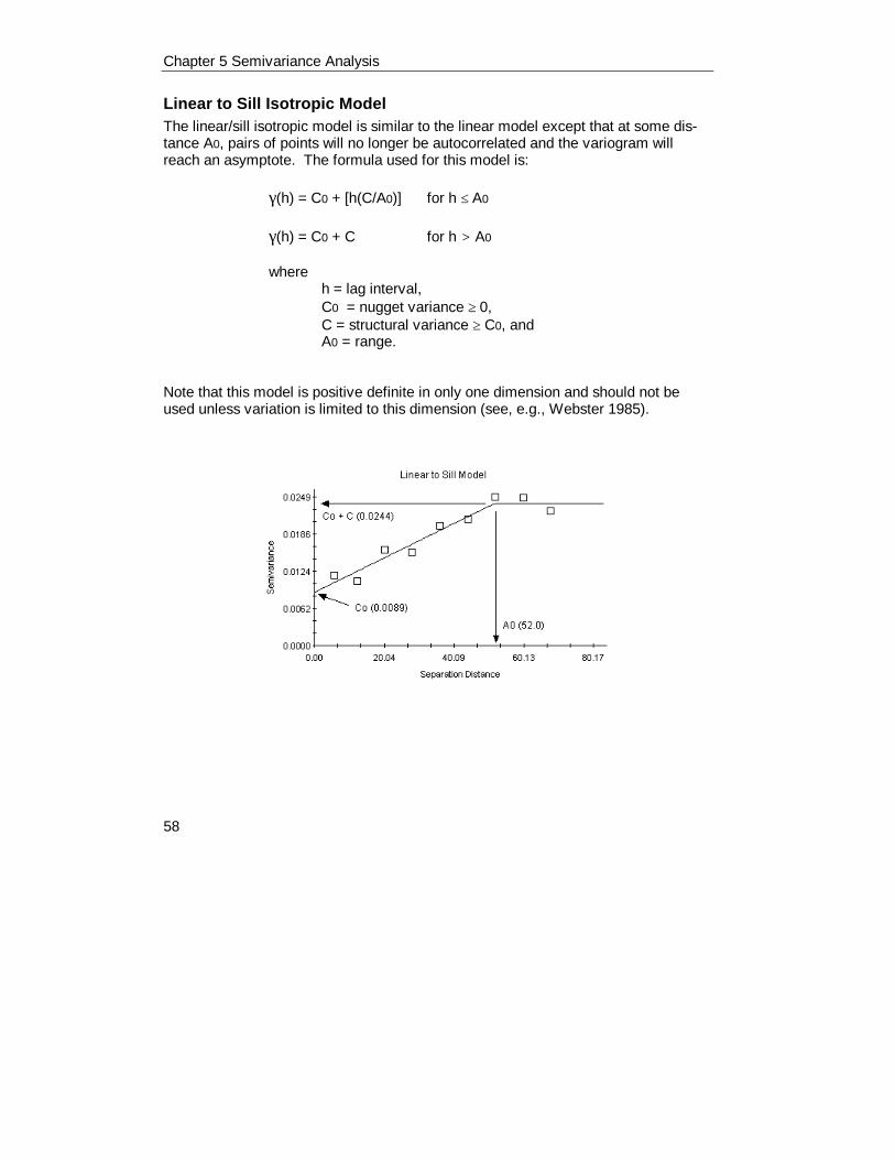
Linear to Sill Isotropic ModelThe linear/sill isotropic model is similar to the linear model except that at some dis-tance A0, pairs of points will no longer be autocorrelated and the variogram willreach an asymptote. The formula used for this model is:
γ(h) = C0 + [h(C/A0)] for h ≤ A0
γ(h) = C0 + C for h > A0
whereh = lag interval,C0 = nugget variance ≥ 0,C = structural variance ≥ C0, andA0 = range.
Note that this model is positive definite in only one dimension and should not beused unless variation is limited to this dimension (see, e.g., Webster 1985).

Chapter 5 Semivariance Analysis
59
Gaussian Isotropic ModelThe gaussian or hyperbolic isotropic model is similar to the exponential model butassumes a gradual rise for the y-intercept. The formula used for this model is:
γ(h) = C0 + C[1-exp(-h2/A02)]
whereh = lag interval,C0 = nugget variance ≥ 0,C = structural variance ≥ C0, andA0 = range parameter (not range).
As for A0 in the exponential model, A0 in the gaussian model is not the range butrather a parameter used in the model to provide range. Range to 95% of the sill inthe gaussian model can be estimated as 3A0.

Chapter 5 Semivariance Analysis
60
Anisotropic Variogram WindowThe Anisotropic Variogram window presents a full-window variogram that can beedited and printed for each anisotropic direction. Additionally, the semivariance val-ues that were used to produce each variogram can be listed, and Variance CloudAnalysis provides a means for detecting outlier pairs of points that may be artificiallyskewing the variogram. Note that the mouse can be used to identify the number ofpairs in specific lag classes (reported at the bottom of the window), and to beginvariance cloud analysis.
List ValuesBring up an Anisotropic Semivariance Values window, including for each directionallag class the average separation distance for pairs of points in that class, the aver-age semivariance for those points, and the number of pairs of points upon which theaverage distance and semivariance are based.
Graph CloudCreate a Variance Cloud Graph window.
Edit GraphBring up a Graph Settings dialog window for editing the graph.
Print GraphPrint the graph via a Graph Print dialog window.

Chapter 5 Semivariance Analysis
61
Anisotropic Semivariance ValuesIn this worksheet are listed for each lag class the average separation distance forpairs of points in that distance and direction class, the average semivariance forthose points, and the number of pairs of points upon which the average distance andsemivariance are based.
PrintPrint the worksheet.
CopyCopies the worksheet values to the Windows clipboard. From the clipboard the val-ues can be pasted into another Windows application.
DecimalsChanges the number of places past the decimal point that are displayed in the col-umns holding non-integer values. Changing the decimals has no effect on the inter-nal storage of values, it affects only their display in this worksheet.
ExitExit the Semivariance Values window.

Chapter 5 Semivariance Analysis
62
Anisotropic Variogram ModelsGS+ provides five types of anisotropic or direction-dependent geometric models,each of which can be described based on four parameters:
• Nugget Variance or Co – the y-intercept of the model; this value is the samefor all directions.
• Sill or Co+C – the model asymptote; this value is the same for all directions.• Range or A – the distance over which spatial dependence is apparent for
the direction examined. It is the sum of:• A1 – the range parameter for the major axis of variation φ• A2 - the range parameter for the minor axis (φ + 90)
Adjusted for the angle between pairs θ as noted in the formulas for indi-vidual models, below.

Chapter 5 Semivariance Analysis
63
GS+ calculates default values for each parameter of the five models. You maychange any of these four model parameters from the Anisotropic Variogram Modeldialog window:
ModelChoose one of the five isotropic models specified. As a model is chosen the vario-gram graphs will be updated to denote the change:
• Spherical• Exponential• Linear• Linear to sill• Gaussian
Model ParametersAny of the three model parameters for each model may be changed within theranges allowed for individual parameters. In addition to the three model parametersnugget, sill, and range, GS+ provides three statistics to aid the interpretation ofmodel output:
• Proportion of Spatial Structure or C/(Co+C) -- this statistic provides a meas-ure of the proportion of sample variance (Co+C) that is explained by spa-tially structured variance C.
• R2 or Regression Coefficient – provides an indication of how well the modelfits the variogram data; this value is not as sensitive or robust as the RSSvalue below for best-fit calculations; use RSS to judge the effect of changesin model parameters.
• RSS or Reduced Sums of Squares – provides an exact measure of how wellthe model fits the variogram data; the lower the reduced sums of squares,the better the model fits. GS+ uses RSS to choose parameters for each of

Chapter 5 Semivariance Analysis
64
the variogram models by determining the combination of parameter valuesthat minimizes RSS for any given model.
ApplyAfter making changes to individual parameters you may apply the changes withoutclosing the dialog window.
CancelExit the dialog window without applying changes since the last Apply command.
ExitClose the dialog window and apply any changes made to individual models.

Chapter 5 Semivariance Analysis
65
Spherical Anisotropic ModelThe spherical anisotropic model is a modified quadratic function in which at somedistance A1 along the major axis and A2 along the minor axis, pairs of points are nolonger autocorrelated and the variogram reaches an asymptote. The formula usedfor this model is:
γ(h) = C0 + C[1.5(h/A)-0.5(h/A)3] for h ≤ A
γ(h) = C0 + C for h > A
whereh = lag interval,C0 = nugget variance ≥ 0,C = structural variance ≥ C0, andA = √ {A1
2[cos2(θ -φ)] + A22[sin2(θ -φ)]}
A1 = range parameter for the major axis (φ)A2 = range parameter for the minor axis (φ + 90)φ = angle of maximum variationθ = angle between pairs

Chapter 5 Semivariance Analysis
66
Exponential Anisotropic ModelThe exponential anisotropic model is similar to the spherical in that it approaches thesill gradually, but different from the spherical in the rate at which the sill is ap-proached and in the fact that the model and the sill never actually converge. Theformula used for this model is:
γ(h) = C0 + C[1-exp(-h/A)]
whereh = lag interval,C0 = nugget variance ≥ 0C = structural variance ≥ C0
A = √ {A12[cos2(θ -φ)] + A2
2[sin2(θ -φ)]}A1 = range parameter for the major axis (φ)A2 = range parameter for the minor axis (φ + 90)φ = angle of maximum variationθ = angle between pairs
Note that A is not the range but rather a parameter used in the model to providerange. It is thus inappropriate to compare A calculated for the exponential model toA’s of nonexponential models. Range in the exponential model is assumed to bethe point at which the model includes 95% of the sill (C+C0); this can be estimatedas 3A1 for the major axis and 3A2 for the minor.

Chapter 5 Semivariance Analysis
67
Linear Anisotropic ModelThe linear anisotropic model describes a straight-line variogram. Note that there isno sill in this model; the ranges for the major and minor axes are defined in terms ofthe distance interval for the last lag class in the variogram. The formula used is:
γ(h) = C0 + h(C/A)
whereh = lag interval,C0 = nugget variance ≥ 0,C = structural variance ≥ C0, andA = √ {A1
2[cos2(θ -φ)] + A22[sin2(θ -φ)]}
A1 = range parameter for the major axis (φ)A2 = range parameter for the minor axis (φ + 90)φ = angle of maximum variationθ = angle between pairs

Chapter 5 Semivariance Analysis
68
Linear to Sill Anisotropic ModelThe linear/sill model is similar to the linear model except that at some distance A1 forthe major axis and A2 for the minor axis, pairs of points are no longer autocorrelatedand the semivariogram reaches an asymptote. The formula used for this model is:
γ(h) = C0 + [h(C/A)] for h ≤ A
γ(h) = C0 + C for h > A
whereh = lag interval,C0 = nugget variance ≥ 0,C = structural variance ≥ C0, andA = √ {A1
2[cos2(θ -φ)] + A22[sin2(θ -φ)]}
A1 = range parameter for the major axis (φ)A2 = range parameter for the minor axis (φ + 90)φ = angle of maximum variationθ = angle between pairs
Note that this model is positive definite in only one dimension and should not beused unless variation is limited to this dimension (see, e.g., Webster 1985).

Chapter 5 Semivariance Analysis
69
Gaussian Anisotropic ModelThe gaussian or hyperbola anisotropic model is similar to the exponential model butassumes a gradual rise from the y-intercept. The formula used for this model is:
γ(h) = C0 + C[1-exp(-h2/A2)]
whereh = lag interval,C0 = nugget variance ≥ 0,C = structural variance ≥ C0, andA = √ {A1
2[cos2(θ -φ)] + A22[sin2(θ -φ)]}
A1 = range parameter for the major axis (φ)A2 = range parameter for the minor axis (φ + 90)φ = angle of maximum variationθ = angle between pairs

Chapter 5 Semivariance Analysis
70

Chapter 6 Fractal Analysis
71
Chapter 6Fractal AnalysisThe Fractal Analysis window is used to set up the parameters for fractal analysisand then calculate the fractal dimension D for the data set defined in the Data Defi-nition Menu. GS+ calculates the fractal dimension D as a function of the slope of alog-log semivariogram plot (Burrough 1981, 1986 ):
D = 2 - m / 2
whereD = the Hausdorff-Besicovitch statistic,m = the slope of a log-log semivariogram.
Because D is based on an analysis of semivariance, it is sensitive to the sameanalysis parameters that affect semivariance analysis.
Fractal analysis is performed from both an isotropic (direction independent) and ani-sotropic (direction-dependent) perspective. The window below has the isotropic tabrather than the anisotropic tab selected:
Active Lag DistanceThe Active Lag Distance specifies the range over which semivariance will be calcu-

Chapter 6 Fractal Analysis
72
lated. The minimum distance for this field is the minimum distance between adjacentpoints in the data set, while the maximum distance is the maximum distance be-tween points.
For example, a 1200 m transect will have a maximum lag of 1200 m; specifying anActive Lag of 300 m will limit the variogram to lag intervals less than or equal to 300m along the entire 1200 m length of the transect.
The default active lag is 80% of the maximum lag. This is not likely to be the mostappropriate active lag for your data but rather will provide a starting point. Vario-grams typically decompose at large lag intervals because of decreasing numbers ofcouples per lag class as the maximum lag interval is approached.
GS+ allows 1 million lag classes to be specified with up to 1 billion pairs per class.
Changing the Active Lag in the Fractal Analysis window will also change the ActiveLag in the Moran’s I Analysis window and in the Semivariance Analysis Window,and vice versa.
Lag Class Distance IntervalThe Lag Class Distance Interval defines how pairs of points will be grouped into lagclasses. Each point in an autocorrelogram represents the average ln(semivariance)for a single lag class, which is a group of pairs separated by a certain Lag ClassDistance Interval, sometimes called a step size. This interval can either be calcu-lated by GS+, in which case it will be uniformly distributed across the active lag dis-tance, or it can be manually set by the user:
Use individually-specified pointsWith this option you may use the Define command to bring up a window to DefineLag Class Intervals, i.e. to specify individual break points for the lag intervals.
Use a uniform intervalWith this option, the value specified is the size of the interval, applied uniformlyacross the active lag distance. E.G. an interval of 2 units with an active lag distanceof 10 units will create 5 lag classes, each 2 units wide. The minimum interval al-lowed is the smallest distance separating any two sample point locations in the dataset. The maximum interval is the greatest distance separating any two sample pointlocations. The default value is 10% of the active lag or, if 10% of the active lag issmaller than the minimum allowed, the minimum allowed. This default may not beappropriate for any given data set; you should try different steps for every set.

Chapter 6 Fractal Analysis
73
The number of lag classes (and therefore plotted points) in a log-log variogram is afunction of values for the active lag and the active step; a 300 m active lag with a 15m active step will have ca. 20 lag classes. Note, however, that the lag distance for agiven class will be the average distance separating points within the class and notnecessarily the midpoint for the class. For a 10-20 m lag class, e.g., the average lagdistance may be 12.3 m rather than 15 m if more pairs of points are separated by10-15 m intervals than by 15-20 m intervals.
Changing the distance interval will clear results on the screen from previous analy-ses calculated with a different step. Results based on the new step must be re-generated with Calculate command.
Note also that changing the distance interval on the Fractal Analysis window willalso change the distance interval in the Semivariance Analysis window and in theMoran’s I Analysis window, and vice versa.
Anisotropic Axis OrientationAnisotropy refers to a direction-dependent trend in the data. Consider data collectedfrom a two-dimensional grid on a mountain slope: elevation will be autocorrelateddifferently in the upslope - downslope direction than in a cross-slope direction, andthus an isotropic (all-direction) analysis may hide much of the autocorrelation that infact is present. Anisotropic analysis allows you to see if your data have a directionalcomponent that might arise from a variety of unforeseen factors. Anisotropic analy-sis is irrelevant for single-dimension data such as a transect or a time series.
Principal Axis (degrees N)The Principal Axis is the base axis from which the offset angles for anisotropicanalyses are calculated. Offset angles are 0°, 45°, 90°, and 135° clockwise fromthe base axis; points aligned sufficiently close to one or another of these angles (seeOffset Tolerance below) are included in the anisotropic analysis for that angle.
The axis orientation should correspond to the axis of maximum variation; the defaultaxis is 0° from the north-south (y) axis.
Offset Tolerance (degrees)In anisotropic analyses, the Offset Tolerance determines how closely the alignmentbetween any two points needs to be for those points to be included in the analysisfor a given offset angle. Two points will be included in the analysis for a given offsetangle if the angle between them is within the offset tolerance from the offset angle.
For example, if the angle between two points is 59.3° and the offset tolerance is15.0°, the points will be included only in the 45° angle class, which would include all

Chapter 6 Fractal Analysis
74
angles between 30° and 60°. The default tolerance is 22.5°.
EnlargeThe Enlarge command brings up a separate Fractal Analysis window, from whichthe log-log variogram can be printed or formatted. Also available from the FractalAnalysis Window is Variance Cloud Analysis and the ability to view individual log-logsemivariance values and the number of pairs per variogram class interval.
CalculateThe Calculate command causes the fractal analysis to be performed.
ExitThe Exit command closes the Fractal Analysis Window.

Chapter 6 Fractal Analysis
75
Isotropic Fractal VariogramThe Isotropic Fractal Variogram window presents a full-window log-log variogramthat can be edited and printed. Additionally, the semivariance values that were usedto produce the variogram can be listed, and Variance Cloud Analysis provides ameans for detecting outlier pairs of points that may be artificially skewing the vario-gram. Note that the mouse can be used to identify the number of pairs in specific lagclasses (reported at the bottom of the window), and to begin variance cloud analy-sis.
List ValuesBring up an Fractal Variogram Values window, including for each lag class the aver-age separation distance for pairs of points in that class, the ln(average semivari-ance) for those points, and the number of pairs of points upon which the averagedistance and ln(average semivariance) are based.
Graph CloudCreate a Cloud Variance Graph window.
Edit GraphBring up a Graph Settings dialog window for editing the graph.
Print GraphPrint the graph via a Graph Print dialog window.

Chapter 6 Fractal Analysis
76
Isotropic Fractal Variogram ValuesIn this worksheet are listed for each isotropic lag class the average separation dis-tance for pairs of points in that class, the average ln(semivariance) value for thosepoints, and the number of pairs of points upon which the average distance andln(semivariance) value are based.
PrintPrint the worksheet. Data can be printed to a file for export.
CopyCopies the worksheet values to the Windows clipboard. From the clipboard the val-ues can be pasted into another Windows application.
DecimalsChanges the number of places past the decimal point that are displayed in the col-umns holding non-integer values. Changing the decimals has no effect on the inter-nal storage of values, it affects only their display in this worksheet.
ExitClose the Autocorrelogram Listing window.

Chapter 6 Fractal Analysis
77
Fractal Analysis - Anisotropic ModelFractal analysis is performed from both an isotropic (direction independent) and ani-sotropic (direction-dependent) perspective. The window below has the anisotropictab rather than the isotropic tab selected; see the Isotropic Fractal Analysis windowfor a description of the commands and fields.

Chapter 6 Fractal Analysis
78
Anisotropic Fractal VariogramThe Anisotropic Fractal Variogram window presents for each anisotropic direction afull-window log-log variogram that can be edited and printed. Additionally, the semi-variance values that were used to produce the variogram can be listed, and Vari-ance Cloud Analysis provides a means for detecting outlier pairs of points that maybe artificially skewing the variogram. Note that the mouse can be used to identify thenumber of pairs in specific lag classes (reported at the bottom of the window), and tobegin variance cloud analysis.
List ValuesBring up an Fractal Variogram Values window, including for each lag class the aver-age separation distance for pairs of points in that class, the averageln(semivariance) for those points, and the number of pairs of points upon which theaverage distance and ln(semivariance) are based.
Graph CloudCreate a Cloud Variance Graph window.
Edit GraphBring up a Graph Settings dialog window for editing the graph.
Print GraphPrint the graph via a Graph Print dialog window.

Chapter 6 Fractal Analysis
79
Anisotropic Fractal Variogram ValuesIn this worksheet are listed for each directional lag class the average separationdistance for pairs of points in that class, the average ln(semivariance) value forthose points, and the number of pairs of points upon which the average distance andln(semivariance) value are based.
PrintPrint the worksheet. Data can be printed to a file for export.
CopyCopies the worksheet values to the Windows clipboard. From the clipboard the val-ues can be pasted into another Windows application.
DecimalsChanges the number of places past the decimal point that are displayed in the col-umns holding non-integer values. Changing the decimals has no effect on the inter-nal storage of values, it affects only their display in this worksheet.
ExitClose the Autocorrelogram Listing window.

Chapter 6 Fractal Analysis
80

Chapter 7 Moran’s Autocorrelation Analysis
81
Chapter 7Moran’s I Autocorrelation Analysis
The Moran’s I statistic is a conventional measure of autocorrelation, similar in inter-pretation to the Pearson’s Product Moment correlation statistic for independentsamples in that both statistics range between -1.0 and 1.0 depending on the degreeand direction of correlation.
The statistic is defined as:
I(h) = N(h) Σ Σ zi zj / Σ zi 2
whereI(h) = autocorrelation for interval distance class h;zi = the measured sample value at point i;zj = the measured sample value at point i+h.
Note that in this analysis all of the weights in the adjacency matrix (Sokal and Oden1978) are set to 1, i.e. I is weighted by distance (h) between sample points ratherthan by simple adjacency. Calculating this statistic for a variety of lag distancesproduces an autocorrelogram such as that pictured below.
Autocorrelation is evaluated in GS+ by calculating I(h) for all possible pairs of pointsin the data set and assigning each pair to a distance interval class h. For uniforminterval classes, GS+ makes interval class assignments for any given pair of pointsusing the following formula:
class = INT(D/DI)+1
whereD = distance separating the pairDI = lag class distance intervalINT = Integer()
For individually-specified lag class intervals, pairs of points are assigned to intervallag classes based on values in the Define Lag Class Intervals window.
GS+ calculates I for each interval class h; the graph of h vs. I for each interval classin the analysis constitutes the autocorrelogram.
As for semivariance analysis, Moran’s I autocorrelograms are sensitive to analysis

Chapter 7 Moran’s Autocorrelation Analysis
82
parameters such as the lag class distance interval and active lag distance. Youshould consult references noted in the Bibliography (Section 6.0) to gain a theoreti-cal understanding of the analysis. As for semivariograms, you will need to experi-ment with different intervals and lag distances to get a feel for what values are ap-propriate for a particular data set.
Active Lag DistanceThe Active Lag Distance specifies the range over which semivariance will be calcu-lated. The minimum distance for this field is the minimum distance between adjacentpoints in the data set, while the maximum distance is the maximum distance be-tween points.
For example, a 1200 m transect will have a maximum lag of 1200 m; specifying anActive Lag of 300 m will limit the variogram to lag intervals less than or equal to 300m along the entire 1200 m length of the transect.
The default active lag is 80% of the maximum lag. This is not likely to be the mostappropriate active lag for your data but rather will provide a starting point. Autocor-relograms typically decompose at large lag intervals because of decreasing num-bers of couples per lag class as the maximum lag interval is approached.
GS+ allows 1 million lag classes to be specified with up to 1 billion pairs per class.

Chapter 7 Moran’s Autocorrelation Analysis
83
Changing the Active Lag on the Semivariance Screen will also change the ActiveLag in the Moran’s I Analysis window and in the Fractal Analysis window, and viceversa.
Lag Class Distance IntervalThe Lag Class Distance Interval defines how pairs of points will be grouped into lagclasses. Each point in an autocorrelogram represents the average Moran’s I for asingle lag class, which is a group of pairs separated by a certain Lag Class DistanceInterval, sometimes called a step size. This interval can either be calculated by GS+,in which case it will be uniformly distributed across the active lag distance, or it canbe manually set by the user:
Use individually-specified pointsWith this option you may use the Define command to bring up a window to DefineLag Class Intervals, i.e. to specify individual break points for the lag intervals.
Use a uniform intervalWith this option, the value specified is the size of the interval, applied uniformlyacross the active lag distance. E.G. an interval of 2 units with an active lag distanceof 10 units will create 5 lag classes, each 2 units wide. The minimum interval al-lowed is the smallest distance separating any two sample point locations in the dataset. The maximum interval is the greatest distance separating any two sample pointlocations. The default value is 10% of the active lag or, if 10% of the active lag issmaller than the minimum allowed, the minimum allowed. This default may not beappropriate for any given data set; you should try different steps for every set.
The number of lag classes (and therefore plotted points) in an autocorrelogram is afunction of values for the active lag and the active step; a 300 m active lag with a 15m active step will have ca. 20 lag classes. Note, however, that the lag distance for agiven class will be the average distance separating points within the class and notnecessarily the midpoint for the class. For a 10-20 m lag class, e.g., the average lagdistance may be 12.3 m rather than 15 m if more pairs of points are separated by10-15 m intervals than by 15-20 m intervals.
Changing the distance interval will clear results on the screen from previous analy-ses calculated with a different step. Results based on the new step must be re-generated with Calculate command.
Note also that changing the distance interval on the Moran’s I Analysis window willalso change the distance interval in the Semivariance Analysis window and in theFractal Analysis Window, and vice versa.

Chapter 7 Moran’s Autocorrelation Analysis
84
Anisotropic Axis OrientationAnisotropy refers to a direction-dependent trend in the data. Consider data collectedfrom a two-dimensional grid on a mountain slope: elevation will be autocorrelateddifferently in the upslope - downslope direction than in a cross-slope direction, andthus an isotropic (all-direction) analysis may hide much of the autocorrelation that infact is present. Anisotropic analysis allows you to see if your data have a directionalcomponent that might arise from a variety of unforeseen factors. Anisotropic analy-sis is irrelevant for single-dimension data such as a transect or a time series.
Principal Axis (degrees N)The Principal Axis is the base axis from which the offset angles for anisotropicanalyses are calculated. Offset angles are 0°, 45°, 90°, and 135° clockwise fromthe base axis; points aligned sufficiently close to one or another of these angles (seeOffset Tolerance below) are included in the anisotropic analysis for that angle.
The axis orientation should correspond to the axis of maximum variation; the defaultaxis is 0° from the north-south (y) axis.
Offset Tolerance (degrees)In anisotropic analyses, the Offset Tolerance determines how closely the alignmentbetween any two points needs to be for those points to be included in the analysisfor a given offset angle. Two points will be included in the analysis for a given offsetangle if the angle between them is within the offset tolerance from the offset angle.For example, if the angle between two points is 59.3° and the offset tolerance is15.0°, the points will be included only in the 45° angle class, which would include allangles between 30° and 60°. The default tolerance is 22.5°.
EnlargeThe Enlarge command brings up a separate Variogram Window, from which thevariogram can be printed or formatted. Also available from the Variogram Window isVariogram Cloud Analysis and the ability to view individual semivariance values andthe number of pairs per variogram class interval.
CalculateThe Calculate command causes the autocorrelogram to be calculated.
ExitThe Exit command closes the Moran’s I Analysis Window.

Chapter 7 Moran’s Autocorrelation Analysis
85
Isotropic AutocorrelogramThe Isotropic Autocorrelogram window presents a full-window correlogram that canbe edited and printed. Additionally, the Moran’s I values that were used to producethe correlogram can be listed, and Variance Cloud Analysis provides a means fordetecting outlier pairs of points that may be artificially skewing the variogram. Notethat the mouse can be used to identify the number of pairs in specific lag classes(reported at the bottom of the window), and to begin variance cloud analysis.
List ValuesBring up an Isotropic Autocorrelogram Values window, including for each lag classthe average separation distance for pairs of points in that class, the average semi-variance for those points, and the number of pairs of points upon which the averagedistance and semivariance are based.
Graph CloudCreate a Cloud Variance Graph window.
Edit GraphBring up a Graph Settings dialog window for editing the graph.
Print GraphPrint the graph via a Graph Print dialog window.
ExitClose the autocorrelogram window.

Chapter 7 Moran’s Autocorrelation Analysis
86
Isotropic Autocorrelogram ValuesIn this worksheet are listed for each lag class the average separation distance forpairs of points in that class, the average Moran’s I value for those points, and thenumber of pairs of points upon which the average distance and Moran’s I value arebased.
PrintPrint the worksheet.
CopyCopies the worksheet values to the Windows clipboard. From the clipboard the val-ues can be pasted into another Windows application.
DecimalsChanges the number of places past the decimal point that are displayed in the col-umns holding non-integer values. Changing the decimals has no effect on the inter-nal storage of values, it affects only their display in this worksheet.
ExitClose the Autocorrelogram Listing window.
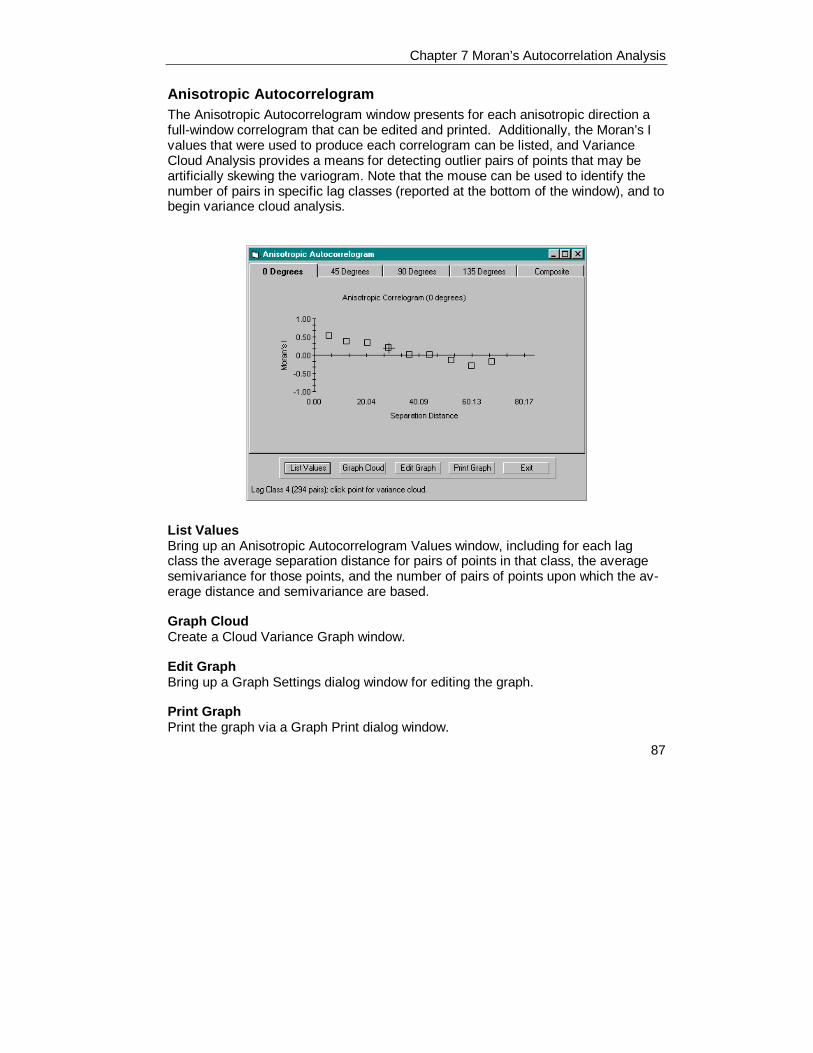
Chapter 7 Moran’s Autocorrelation Analysis
87
Anisotropic AutocorrelogramThe Anisotropic Autocorrelogram window presents for each anisotropic direction afull-window correlogram that can be edited and printed. Additionally, the Moran’s Ivalues that were used to produce each correlogram can be listed, and VarianceCloud Analysis provides a means for detecting outlier pairs of points that may beartificially skewing the variogram. Note that the mouse can be used to identify thenumber of pairs in specific lag classes (reported at the bottom of the window), and tobegin variance cloud analysis.
List ValuesBring up an Anisotropic Autocorrelogram Values window, including for each lagclass the average separation distance for pairs of points in that class, the averagesemivariance for those points, and the number of pairs of points upon which the av-erage distance and semivariance are based.
Graph CloudCreate a Cloud Variance Graph window.
Edit GraphBring up a Graph Settings dialog window for editing the graph.
Print GraphPrint the graph via a Graph Print dialog window.

Chapter 7 Moran’s Autocorrelation Analysis
88
Anisotropic Autocorrelogram ValuesIn this worksheet are listed for each directional lag class the average separationdistance for pairs of points in that class, the average Moran’s I value for thosepoints, and the number of pairs of points upon which the average distance andMoran’s I value are based.
PrintPrint the worksheet.
CopyCopies the worksheet values to the Windows clipboard. From the clipboard the val-ues can be pasted into another Windows application.
DecimalsChanges the number of places past the decimal point that are displayed in the col-umns holding non-integer values. Changing the decimals has no effect on the inter-nal storage of values, it affects only their display in this worksheet.
ExitClose the Autocorrelogram Listing window.

Chapter 9 Kriging
89
Chapter 8Variance Cloud Analysis
The variance cloud is a graph of the variances for all individual pairs of points in anautocorrelation analysis. It is particularly useful for discovering outliers that may in-appropriately skew the average value for a lag class. By placing the mouse on topof individual points you can determine which pairs of points in the data set are sus-pect. The records making up a particular variance pair is reported at the bottom ofthe screen; the pair number (e.g. “Pair 171” below) refers to the position of the pairin the pair listing.
Note that a variance cloud is specific to both direction (isotropic or a specific aniso-tropic direction) and to a particular lag class. In the example below the cloud is spe-cific to the second lag class of the isotropic variogram, as noted in the graph title,and the mouse is on top of pair 171, made up of data records 100 and 109, whichare separated by 5.33 distance units.
Lag ClassThe lag class for which the variance cloud is created. The variance for every pair ofpoints in the lag class is plotted against the distance interval separating that pair.
List ValuesBring up a listing of Isotropic Variance Cloud Pairs or Anisotropic Variance CloudPairs, including for each pair the variance, separation distance, and the identity

Chapter 9 Kriging
90
(data record number) of each member of the pair.
Edit GraphBring up a Graph Settings dialog window for editing the graph.
Print GraphPrint the graph via a Graph Print dialog window.
ExitClose the variance cloud window.

Chapter 9 Kriging
91
Isotropic Variance Cloud PairsThis window contains a listing of all pairs of points within a specific lag class. in-cluding for each pair the variance, separation distance, and the identity (data recordnumber) of each member of the pair. These pairs are graphed in the VarianceCloud window.
SortSort values in the worksheet by separation distance or by variance values.
PrintPrint a copy of the worksheet.
CopyCopies the worksheet values to the Windows clipboard. From the clipboard the val-ues can be pasted into another Windows application.
DecimalsChanges the number of places past the decimal point that are displayed in the col-umns holding non-integer values. Changing the decimals has no effect on the inter-nal storage of values, it affects only their display in this worksheet.
ExitClose the worksheet window.

Chapter 9 Kriging
92
Anisotropic Variance Cloud PairsThis window contains a listing of all pairs of points within a specific anisotropic lagclass, including for each pair the variance, separation distance, and the identity(data record number) of each member of the pair. These pairs are graphed in theVariance Cloud window. Note that values in the worksheet are specific to both ananisotropic direction and to a particular lag class.
SortSort values in the worksheet by separation distance or by variance values.
PrintPrint a copy of the worksheet.
CopyCopies the worksheet values to the Windows clipboard. From the clipboard the val-ues can be pasted into another Windows application.
DecimalsChanges the number of places past the decimal point that are displayed in the col-umns holding non-integer values. Changing the decimals has no effect on the inter-nal storage of values, it affects only their display in this worksheet.
ExitClose the worksheet window.

Chapter 9 Kriging
93
Chapter 9KrigingKriging provides a means of interpolating values for points not physically sampledusing knowledge about the underlying spatial relationships in a data set to do so.Semivariograms provide this knowledge. Kriging is based on regionalized variabletheory and is superior to other means of interpolation because it provides an optimalinterpolation estimate for a given coordinate location, as well as a variance estimatefor the interpolation value.
In GS+, kriging produces an output file that is used by the GS+ mapping program.GS+ kriging output can also be read into other mapping programs.
Interpolation GridDefines where to place interpolation estimates – in a uniformly spaced grid across arectangular area or at user-specified locations, in either case with or without masksthat can define areas to include or exclude.
• Uniform Grid (specified intervals)
A grid is defined by a rectangle that has an X-direction length, a Y-directionlength, and for each direction, intervals between the grid intersections. In-terpolation locations are at every grid intersection.

Chapter 9 Kriging
94
The default range is defined by the minimum and maximum X-coordinateand Y-coordinate values, and an interval based on a certain number ofpoints in each direction. For 1-dimensional data sets, there is no y direction.
The grid can be changed with the Define command, which will display anInterpolation Grid dialog window.
• Nonuniform Grid (specified points)
A nonuniform grid is composed solely of interpolation locations specified bythe user. Press Define to bring up an Interpolate Worksheet within whichlocations can be defined or imported from an external text file.
• Include irregular shapes (polygons)
Irregular shapes can be interpolated or excluded from being interpolated bydefining inclusive or exclusive polygons prior to kriging. Press Define tobring up a Polygon Outlines Worksheet within which to define polygons.See Define Polygon Outlines later in this chapter.
q In inclusive polygons, the area within the polygon is kriged.
q In exclusive polygons, the area within the polygon is not krigedor mapped.
Output File NamePress Select to select an existing or new file to which kriging interpolation estimateswill be written. For existing files, you may examine the contents of the file bypressing View.
Output FormatThe format with which GS+ will write estimates to the file can be one of severaltypes. These types are described briefly here and more thoroughly below.
• GS+ (.krg) – in this format a header area defines the interpolation grid, vari-ate names, and other information about the file needed to initiate mappinglater, and the data records include for each X and Y Coordinate location thatis kriged the interpolation or Z-estimate, the standard deviation of the Z-estimate, and the number of neighbors that were used to make the estimate.This format is identical to the older GS+ .blk and .pun formats. See examplebelow.

Chapter 9 Kriging
95
• Surfer (.grd) – in this format a short header area defines informationneeded for mapping, and the data is written as a continuous stream of Z-estimates beginning from a specific corner of the interpolation grid. Thestandard deviation of the estimate and the number of neighbors used forinterpolation are NOT included in this format. This format is compatible withGolden Software’s Surfer mapping program. See example below.
• Arc (.asc) – this is similar to the Surfer format but the header area is for-matted differently and the Z-estimates are written in a pattern that beginsfrom a different corner of the interpolation grid. The standard deviation of theestimate and the number of neighbors used for interpolation are NOT in-cluded in this format. This format is compatible with ESRI’s Arc-Info Geo-graphic Information System. See example below.
Interpolation MethodYou may choose either block or punctual kriging methods for interpolation. Thechoice of block vs. punctual kriging should be made on the basis of sampling designand variate characteristics. If samples were taken to represent an area around theactual sample point (e.g. if soil samples from a small area around the sampling co-ordinate were composited before analysis), then block kriging may be more appro-priate than punctual. If samples were taken to represent point values in a field, or intime, then punctual kriging may be more appropriate.
The discretization grid describes the size of the grid placed around the interpolationpoint when block kriging. The interpolation estimate for that point is based on themean value of estimates for each of the discretization grid points. A single discreti-zation point describes punctual kriging. Larger discretization grids take longer tointerpolate.
Variogram Model TypeThe variogram model used for kriging is defined in the Semivariance Analysis win-dow. Here you may choose either the Isotropic (direction-independent) or Aniso-tropic (direction-dependent) model previously defined.
Search NeighborhoodGS+ interpolates values for a specific location using nearest neighbor valuesweighted by distance and the degree of autocorrelation present for that distance (asdefined by the variogram model). Searches are limited to a certain number of near-est neighbors, and can also be restricted to a particular geographic radius. Thedefault value of 16 nearest neighbors is usually sufficient, with no restrictions placedon radius (in Kriging, neighbors outside of the variogram range are weighted identi-cally and, if significant structural dependence is present, weighted minimally).

Chapter 9 Kriging
96
Specifying more than 16 neighbors can slow interpolation substantially.
CalculatePerform kriging analysis. During analysis values are written to the output file in thespecified format.
Cross-Validate
Perform cross-validation analysis . In cross-validation analysis each measured pointin the spatial domain is individually removed from the domain and its value esti-mated via kriging as though it were never there. In this way a graph can be con-structed of estimated vs. actual values for each sample location in the domain.
ExitClose the Kriging Window.

Chapter 9 Kriging
97
Krig Output and Map Input Files
GS+ Format Krig Output FilesThe GS+ format for Krig output files (which is also the GS+ format for Map input files)contains a number of header records with information about the file, followed byXYZ-style records for each interpolated points. Each data record contains fields foran x-coordinate value, a y-coordinate value (except 1-dimensional transects do notcontain a value for the y-coordinate), an estimated z value for that x-y location, anestimation standard deviation for the estimated z-value, and the number of pairsused in the interpolation for that x-y location. Missing values are denoted by what-ever value is specified in the Prferences window.
q The following listing is for the first 8 coordinates for a standard GS+ krig out-put file:
GS+ Output: Block Kriging Interpolation File v3.0Set: Field 54, Second TierDimensions: 2; Interval source: CalculatedInterpolation interval (x; y): 1.3333; 1.3333X-coor: m east range: 0.00 - 80.00Y-coor: m north range: 0.00 - 80.00Z-est: Pb range: 0.151 - 0.813Z-sd: range: 0.0000 - 0.3655Mean Z-estimate (sd): 0.391 (0.0186)Valid N: 3721; Missing N: 0; Missing Value Indicator: -99X-Coordinate Y-Coordinate Z-Estimate EstStdDev n0.00 0.00 0.431 0.3608 160.00 1.33 0.458 0.3486 160.00 2.67 0.462 0.3329 160.00 4.00 0.466 0.3178 160.00 5.33 0.470 0.3034 160.00 6.67 0.474 0.2900 160.00 8.00 0.478 0.2778 160.00 9.33 0.487 0.2550 16

Chapter 9 Kriging
98
Arc/Info or ArcView FormatThe Arc/Info or ArcView Ascii (.ASC) format for Krig output files (which is also theArc/Info format for Map input files) contains a number of header records containinginformation about the file, followed by a string of z values for each row of the inter-polated grid beginning in a particular corner. Unlike GS+ format files, the standarddeviation of the estimate and the number of neighbors used for interpolation areNOT included in this format. Also for this format, the x and y interpolation intervalsmust be the same (you can set them to be the same from the Interpolation Grid dia-log window). This format is compatible with ESRI’s Arc/Info Geographic InformationSystem.
q The following listing is for the first 200 or so coordinates in a standardArc/Info or ArcView format krig output file:
ncols 376nrows 253xllcorner -185556.375yllcorner -127261.5234375cellsize 1009.975NODATA_value -999
354 314 309 301 286 264 305 306 285 285 268 314 339 306 266 248252 240 256 282 277 289 269 285 277 258 256 282 268 246 250 249245 266 262 287 295 335 325 323 359 369 361 357 394 450 407 409382 409 394 486 510 502 516 546 531 542 572 579 586 594 522 654550 615 678 709 616 533 430 576 507 638 778 769 456 432 576 635778 721 769 869 563 589 640 588 770 833 874 1019 965 933 621 7951131 1044 899 1072 1112 880 910 1069 1088 1071 965 975 902 800543 350 330 376 310 384 418 352 263 205 202 200 200 201 200 198201 201 201 201 201 201 201 201 200 201 201 197 197 197 196 196195 195 198 197 201 264 242 230 210 211 214 220 229 233 245 250262 287 354 425 374 329 330 339 354 374 385 409 496 447 609 703629 783 823 837 913 936 1023 1022 1008 940 980 1108 1037 1006988 960 986 941 953 971 983 937 911 875 862 754 763 754 719 747761 703 713 726 701 680 705 705 737 702 694 695

Chapter 9 Kriging
99
Surfer Grid (.GRD) FormatThe Surfer Grid (.GRD) Krig Output format (or Map Input format) has a shortheader area that provides information needed for mapping, and the data is thenwritten as a continuous stream of Z-estimates beginning from a specific corner of theinterpolation grid. The standard deviation of the estimate and the number of neigh-bors used for interpolation are NOT included in this format. This format is compatiblewith Golden Software’s Surfer mapping program. Note that the Surfer Grid formatis different from the Surfer XYZ format used for input files (see Chapter 3).
q The following listing is for the first 100 or so coordinates in a standardSurfer Grid format file. The first record is a required line of code letters thatidentifies the file as a Surfer grid file. Record two contains the number ofgrid lines along the x axis and y axis, respectively. Record 3 contains theminimum and maximum values of the x-coordinate. Record 4 contains theminimum and maximum values of the y coordinate. Record 5 contains theminimum and maximum values for the z-variate. Records 6+ contain the zvalues organized in row order. Within each row the y-coordinate is constant,and the grid row 1 corresponds to the lowest y-coordinate value and the lastrow corresponds to the hightest y-coordinate. Within each row the z-variatevalues are ordered from low x-coordinate to highest x-coordinate.
DSAA376 253-185556.375 194194.225-127261.523 128262.15281.000 4469.000578 746 1097 1251 581 312 229 229 235 278 292 357 490 9971411 1397 1373 1373 1370 1061 942 1003 1288 1014 785 963934 797 703 924 1035 1071 1257 1775 1800 1520 1460 15201278 1098 915 645 495 450 378 339 342 425 613 1084 12921701 1682 1996 2280 2107 1662 1553 1418 1162 1225 12661735 1674 1550 1800 2015 2240 2158 2328 2262 2173 20461688 1849 1880 2023 2320 2029 2140 2240 2650 2465 23692180

Chapter 9 Kriging
100
Uniform Interpolation GridWith the Uniform Interpolation Grid dialog window you may define the region to bekriged or interpolated as well as the intensity at which the interpolation is to takeplace. This method for specifying interpolate locations is appropriate for interpola-tions at regular intervals across an area; if the interpolations are to be performed atodd locations, use the NonUniform Interpolation Grid. If the outline of the area is acomplex polygon you should still use this dialog but then specify the shape of thepolygon from the Krig window. Note that for 1-dimensional data sets (e.g. transectsor time series) only the X direction is displayed in the dialog window.
Interpolation RangeSpecify the beginning and ending values for the region to be interpolated. The re-gion may exceed the Data Range, which is noted on the right side of the dialog win-dow. Irregularly-shaped areas may be interpolated by specifying polygon masksfrom the Krig window.
The number of decimal places used to define the range is limited to the number ofdecimal places specified for the given coordinate field in the Field Assignment Dia-log of the Data Worksheet Window. Changing the number of decimal places for acoordinate in the Data Worksheet Window changes the number of decimal placesreported here.
Data RangeThis is the range covered by the actual data set; these are read-only values, theycannot be changed by the user from this dialog window.
Distance IntervalSpecify the distance interval between locations within the interpolation range. Adistance interval of 2.0 over a range of 0 to 10.0 means that interpolations will bemade at points 0.0, 2.0, 4.0, 6.0, 8.0, and 10.0. Changing the distance interval willchange the number of points value.

Chapter 9 Kriging
101
Number of PointsThe number of points within the range to be interpolated. For any given range, thenumber of points will be the range divided by the distance interval plus 1. For arange of 0 to 10.0 with a distance interval of 2.0, the number of points will be [(10.0 –0)/2.0] +1 = 6 points at locations 0.0, 2.0, 4.0, 6.0, 8.0, and 10.0.
OptimizeThe Optimize command sets the number of points to 61 for both the X and Y direc-tions (101 points for a single-dimension transect) and calculates the appropriateDistance Interval. The Interpolation Range is not affected.
CancelExit the dialog window without saving changes.
ExitExit the dialog window.

Chapter 9 Kriging
102
NonUniform Interpolation GridSpecify in this worksheet the locations of individual points to be kriged. This methodof specifying interpolate locations is appropriate when locations are not regularlyspaced across the interpolation area. If interpolate locations are regularly spaced,regardless of whether the area is rectangular or a complex polygon, it is usuallymore efficient to use a Uniform Interpolation Grid. Note that with either this NonUni-form Grid or the Uniform Grid polygons can be used to exclude or include specificcomplex shapes; specify the shape of the polygon from the Krig window (see DefinePolygon Outlines later in this chapter).
Block SizeFor Block Kriging, this is the size of the block around each point that will be kriged.For uniform grids, this block is defined as half of the distance to the adjacent inter-polate points. The discretization grid is placed within the box. For Point or PunctualKriging, block size is irrelevant.
ClearClears the worksheet.
ImportThe Import command brings into the worksheet a text file containing interpolate lo-cations. The text file can be formatted in a variety of ways. Header records are ini-tial records containing non-numeric data that are ignored during import. Data rec-ords follow header records (if present) and contain a value for the X-Coordinate fol-

Chapter 9 Kriging
103
lowed by a value for the Y-Coordinate; additional fields are ignored (as is the Y-Coordinate field for 1-dimensional analysis).
The file below describes 6 locations to be interpolated:
line 1: Optional header record 1line 2: Optional header record 2line 3: 2.0, 34.line 4: 4.0, 36.line 5: 8.0, 19line 6: 64.0, 34.line 7: 30.0. 35line 8: 10.0, 12.3
CopyCopies the worksheet values to the Windows clipboard. From the clipboard the val-ues can be pasted into another Windows application.
DecimalsChanges the number of places past the decimal point that are displayed in the col-umns holding non-integer values. Changing the decimals has no effect on the inter-nal storage of values, it affects only their display in this worksheet.
PrintPrint the worksheet
ExitExit and close the dialog window.

Chapter 9 Kriging
104
Define Polygon OutlinesIrregular shapes can be interpolated or excluded from being interpolated by defininginclusive or exclusive polygons prior to kriging. In this window you can define thepolygons to be used by entering coordinates of polygon vertices, i.e. the coordinatepairs that define the polygon outline.
Polygons must be closed, thus they must have at least 3 vertices (3 vertices de-scribe a triangle). You may specify as many vertices per polygon as you like (up toseveral billion), and polygons may be nested within one another as in the examplebelow. Be aware, however, that the vertices for each polygon must define a single,closed polygon, i.e. no segments of the polygon may cross another segment. Alsobe aware that the first and last vertex specified connect to one another. You cancheck the shape of the polygon while it is being defined with the Map command.
There are two types of polygons, defined by the keyword “Include” and “Exclude” inthe worksheet as noted in the example below:
• In inclusive polygons, the area within the polygon is kriged.• In exclusive polygons, the area within the polygon is not kriged.
The example below defines two polygons: the first is a 6-sided area that is excludedfrom interpolation, the second defines an inclusive 4-sided area (rectangle) insidethe 6-sided area. You can use the Map command to produce a picture of thesepolygons (see below). The first line in this example (“Polygon”) is unnecessary.

Chapter 9 Kriging
105
ClearClear the worksheet.
ImportThe Import command brings into the worksheet a text file containing vertex loca-tions. The text file can be formatted in a variety of ways with fields separated byeither commas or spaces.
PrintPrint the worksheet.
MapProduces an outline map of each polygon within the larger interpolation grid area.Exclusive polygons appear in red, inclusive in blue. See the example in the nextsection.
CopyCopies the worksheet values to the Windows clipboard. From the clipboard the val-ues can be pasted into another Windows application.
DecimalsChanges the number of places past the decimal point that are displayed in the col-umns holding non-integer values. Changing the decimals has no effect on the inter-nal storage of values, it affects only their display in this worksheet.
ExitExit and close the Define Polygon window.

Chapter 9 Kriging
106
Polygon Outline MapThis window contains an outline map of the polygons used to include and excludeareas from kriging. It is accessed from the Define Polygon Outlines window, whichis part of Kriging analysis.
The overall area is the interpolation area specified in the Kriging window. Polygonsare defined in the Define Polygon Outlines worksheet. Exclusive polygons appear inred, inclusive in blue.
Edit GraphMake format and text changes to the graph via a Graph Settings dialog window.
Print GraphPrint the graph to a printer or file with the Graph Print dialog window.
ExitClose the window and exit.

Chapter 9 Kriging
107
Cross-Validation AnalysisCross-validation analysis is a means for evaluating alternative models for kriging. Incross-validation analysis each measured point in a spatial domain is individually re-moved from the domain and its value estimated via kriging as though it were neverthere. In this way a graph can be constructed of the estimated vs. actual values foreach sample location in the domain.
Each point on the graph represents a location in the input data set for which an ac-tual and estimated value are available. Information about individual points is pro-vided at the bottom of the screen; points are displayed by placing the cursor onthem; in the case above the cursor was placed about the point representing record116.
The regression coefficient at the bottom of the graph represents a measure of thegoodness of fit for the least-squares model describing the linear regression equa-tion. A perfect 1:1 fit would have a regression coefficient (slope) of 1.00 and thebest-fit line (the blue line in the graph above) would coincide with the dotted 1:1 lineon the graph. The standard error (SE = 0.520, above) refers to the standard error of

Chapter 9 Kriging
108
the regression coefficient; the r2 value is the proportion of variation explained by thebest-fit line (in this case 39.9%; it is the square of the correlation coefficient); and they-intercept of the best-fit line is also provided.
List ValuesShow a separate worksheet of the values used to make the graph.
Edit GraphMake format and text changes to the graph via a Graph Settings dialog window.
Print GraphPrint the graph to a printer or file with the Graph Printing dialog window.
ExitClose the window and exit.

Chapter 9 Kriging
109
Cross-Validation ValuesIn cross-validation analysis each measured point in a spatial domain is individuallyremoved from the domain and its value estimated via kriging as though it were neverthere. Results can be graphed as well as listed in a table such as that below.
TableThe record number refers to the actual record in the Data Worksheet. For each rec-ord successfully kriged the actual Z value is presented in the middle column and theestimated Z value is provided to its right.
PrintPrint the worksheet
CopyCopies the worksheet values to the Windows clipboard. From the clipboard the val-ues can be pasted into another Windows application.

Chapter 9 Kriging
110
DecimalsChanges the number of places past the decimal point that are displayed in the col-umns holding non-integer values. Changing the decimals has no effect on the inter-nal storage of values, it affects only their display in this worksheet.
ExitExit and close the dialog window.

Chapter 10 Mapping
111
Chapter 10MappingGS+ produces 2d and 3d maps of spatial data following kriging. The data to bemapped come from kriging analysis, and are thus contained in krig output files.Maps can be displayed in a variety of ways with a variety of different contouringschemes, 3-dimensional maps can be rotated on the fly, and both 2-dimensional and3-dimensional maps can be zoomed to more closely view a transition or other mapfeature. Additionally, sample postings (original data locations) can be displayed,and estimation standard deviations can be mapped for input files that have beensaved in the standard GS+ format.
Map Input File• Select – allows you to choose the file with the data to be mapped. The de-
fault file extension will correspond to the selected file format (e.g. .krg, .blk,and .pun for GS+ format), although a file with any extension can be selected.
• View – view the selected file in the View File window.• Format – specify the format to use to read the input file. Files with a .krg,
.blk, or .pun extension are assumed to be in GS+ format, as are files withother specific extensions. The format specified in this field will override anyassumed format.

Chapter 10 Mapping
112
Map Grid• X direction – the range within the file for values in the x (horizontal) direc-
tion.• Y direction – the range within the file for values in the y (vertical) direction;
for 1-dimensional data sets this field is blank.• Z values – the range of estimated Z values in the input file.• Z SD values – the range of estimation Z standard deviation values in the
input file; only files in the GS+ format contain both Z values and Z standarddeviation values..
• N (N missing) – the number of valid records in the file and (in parentheses)the number of missing values . The default missing value indicator (e.g. –999.) is specified in the Configuration window; the active missing value indi-cator for map files is indicated in the Map Contour Intervals window. Miss-ing values are mapped as transparent regions. Exclusive polygons aremapped as missing values, as is any interpolate location for which there isno kriging solution.
Variate to Map• Z values – maps the estimated Z values in the file• Z standard deviations – maps the estimation Z standard deviations in the
file; only files in the GS+ format contain both Z values and Z standard devia-tion values.
• Sample Posting – map only the original sample locations. Requires thepresence of a posting file, which has the same name as the input file but a.pos extension. This file is created during kriging; if it is not present you willnot be able to map a sample posting.
Graph Type• 2-d – displays a flat, 2-dimensional map of the data• 3-d – displays a 3-dimensional map of the data. The height of the map can
be adjusted with the Edit Graph command of the Map window; the perspec-tive can be adjusted with the Rotate command of the Map window.
• 1-d – displays 1-dimensional data (e.g. a geographic transect or a time se-ries) as an x-y graph. This choice is not available for 2-dimensional data.
• Show legend – displays the contour legend next to the map.

Chapter 10 Mapping
113
Surface• Contour lines – draws lines between contour intervals• Color bands – fills the space between contour lines with different colors;
colors can be specified from the Define Contour dialog window by pressingDefine Contour Levels, below.
• Smoothing – apply slight smoothing to the data to improve visualization.• Solid pedestal – for a 3-d map fill in the area beneath the surface with a
solid color.• Wireframe – for 3-d maps, drapes an x-y grid over the surface.• Wireframe Weave – specifies the density of the wireframe grid. A weave of
0 puts a grid line at every data row and column; a weave of 1 skips onerow/column, a weave of 2 skips 2, etc.
Contour Levels• Number – the number of contour levels to put on the map.• Define – brings up the Map Contour Intervals dialog window that allows you
to set break points for individual intervals and colors for contour bands.
Ceiling• Contour lines – project contour lines above the plot surface (3d maps only).• Color bands – project color bands onto the ceiling of the plot (3d maps only).
Floor• Contour lines – project contour lines under the plot surface (3d maps only).• Color bands – project color bands onto the floor of the plot (3d maps only).
Grid Lines• X axis – place a vertical grid line along the back walls of the 3d plot x axis.• Y axis – place a vertical grid line along the back wall of the 3d plot y axis.• Z axis – place horizontal grid lines along the back walls of 3d plots.
DrawCreate the map in a Map Image window.
ExitClose the Map window and exit.

Chapter 10 Mapping
114
Map Contour IntervalsThis dialog window allows one to specify the break points and colors for the contourintervals used for mapping. The number of contour intervals is specified in the Mapwindow, where access to this Map Contour Intervals window is provided.
Contour Intervals• Color buttons – change the color of a specified interval by clicking the adja-
cent color button.• Break points – change the break point between adjacent contour intervals
by providing a new value in the space provided. Note that the new breakpoint must be greater than the preceding point and less than the one thatfollows.
• Missing value – specify the missing value indicator for the data file. Thisvalue is usually embedded in the input file as part of the header information,and is automatically extracted by GS+.

Chapter 10 Mapping
115
Intervals• Get – read contour intervals from a text file; the first value of each record of
line of the file is presumed to be a separate interval.• Save – save the existing contour intervals to a text file.• Reset – recalculate intervals based on a uniform distribution (even intervals)
between the lowest and highest value in the file.
Color Source• Standard – specifies a default color pattern of red-orange-yellow… .. violet.• Blue – specifies a default color pattern of different shades of blue.• Custom – specifies a custom color pattern defined below.• Red – specifies a default color pattern of different shades of red.• Green – specifies a default color pattern of different shades of green.• Gray – specifies a default color pattern of different shades of gray.
Color Source Custom• Get – get a custom color pattern saved earlier. The initial custom color is
the same as the standard color source, above.• Save – save the existing color pattern as the custom color pattern.• Reset – reset the custom color pattern to the default Standard pattern.
CancelExit the dialog window without saving changes.
ExitExit and save changes.

Chapter 10 Mapping
116
Map Image - 3DThe 3D map image is produced by the Draw command from the Mapping window.
Edit GraphChange axis scales, titles, and numeric formats via the Graph Settings dialog win-dow.
Print GraphPrint the active graph to a file, printer, or other device via the Graph Print dialog win-dow.
ExitExit and close the Map Image window.

Chapter 10 Mapping
117
Mouse Action• Off – returns the mouse to normal operation.• Rotate – turns the cursor into a rotator cuff when the left mouse button is
pushed, allowing the image to be rotated as desired.• Move – allows the graph to be moved within the window by clicking the left
mouse button and dragging the cursor.• Scale – shrinks the graph image with the left mouse button.• Zoom – allows you to zoom in on a particular graph area by using the left
mouse button to define a rectangular zoom area. Within the zoomed areathe location of the cursor is noted on the Mouse Location panel.
• Reset – resets the image to the default rotation angle and scale.
Mouse LocationProvides information on the current location of the cursor when it is on the map sur-face. Units are map units as specified by the axes.

Chapter 10 Mapping
118
Map Image - 3D Standard DeviationsA map of standard deviations can be produced for kriged files that are saved in GS+
format; use the Draw command from the Mapping window.
Edit GraphChange axis scales, titles, and numeric formats via the Graph Settings dialog win-dow.
Print GraphPrint the active graph to a file, printer, or other device via the Graph Print dialog win-dow.
ExitExit and close the Map Image window.

Chapter 10 Mapping
119
Mouse Action• Off – returns the mouse to normal operation.• Rotate – turns the cursor into a rotator cuff when the left mouse button is
pushed, allowing the image to be rotated as desired.• Move – allows the graph to be moved within the window by clicking the left
mouse button and dragging the cursor.• Scale – shrinks the graph image with the left mouse button.• Zoom – allows you to zoom in on a particular graph area by using the left
mouse button to define a rectangular zoom area. Within the zoomed areathe location of the cursor is noted on the Mouse Location panel.
• Reset – resets the image to the default rotation angle and scale.
Mouse LocationProvides information on the current location of the cursor when it is on the map sur-face. Units are map units as specified by the axes.

Chapter 10 Mapping
120
Map Image - 3D RotationThree-dimensional map images can be rotated to any viewing angle. To rotate,choose Rotate on the Mouse Action panel of the Map Image window, and holddown the left-mouse button while moving the mouse over the graph. The cursorwill be replaced with a 3d box (see figure below) describing the viewing angle thathas been selected. Release the mouse and the map will be drawn (as in thesecond figure below).

Chapter 10 Mapping
121
This is how the newly-rotated graph looks.

Chapter 10 Mapping
122
Map Image - 2DThe 2D map image is produced by the Draw command from the Mapping windowwhen the Graph Type within that window is set to 2d.
Edit GraphChange axis scales, titles, and numeric formats via the Graph Settings dialog win-dow.
Print GraphPrint the active graph to a file, printer, or other device via the Graph Print dialog win-dow.
ExitExit and close the Map Image window.
Chapter 10 Mapping
123
Mouse Action• Off – returns the mouse to normal operation.• Rotate – for 3D images, turns the cursor into a rotator cuff when the left
mouse button is pushed, allowing the image to be rotated. Not available for2D images.
• Move – allows the graph to be moved within the window by clicking the leftmouse button and dragging the cursor.
• Scale – allows one to use the left mouse button to shrink the graph image.• Zoom – allows the user to zoom in on a particular graph area by using the
left mouse button to define a rectangular zoom area. Within the zoomedarea the location of the cursor is noted on the Mouse Location panel.
• Reset – resets the image to the default rotation angle and scale.
Mouse LocationProvides information on the current location of the cursor when it is on the map sur-face. Units are map units as specified by the axes.

Chapter 10 Mapping
124
Map Image - 2D Standard DeviationsThe 2D standard deviations map image is produced by the Draw command from theMapping window when the Graph Type within that window is set to 2d and the Stan-dard Deviation box is checked.
Edit GraphChange axis scales, titles, and numeric formats via the Graph Settings dialog win-dow.
Print GraphPrint the active graph to a file, printer, or other device via the Graph Print dialog win-dow.
ExitExit and close the Map Image window.

Chapter 10 Mapping
125
Mouse Action• Off – returns the mouse to normal operation.• Rotate – for 3D images, turns the cursor into a rotator cuff when the left
mouse button is pushed, allowing the image to be rotated. Not available for2D images.
• Move – allows the graph to be moved within the window by clicking the leftmouse button and dragging the cursor.
• Scale – allows one to use the left mouse button to shrink the graph image.• Zoom – allows the user to zoom in on a particular graph area by using the
left mouse button to define a rectangular zoom area. Within the zoomedarea the location of the cursor is noted on the Mouse Location panel.
• Reset – resets the image to the default rotation angle and scale.
Mouse LocationProvides information on the current location of the cursor when it is on the map sur-face. Units are map units as specified by the axes.

Chapter 10 Mapping
126
Map Image - 2D Sample Posting
The 2D sample posting is produced by the Draw command from the Mapping win-dow when the Graph Type within that window is set to 2d and the Posting box ischecked. Each “X” symbol in the image below marks an actual sample location asdefined by the original X,Y coordinate locations in the Data Worksheet window.
Edit GraphChange axis scales, titles, and numeric formats via the Graph Settings dialog win-dow.
Print GraphPrint the active graph to a file, printer, or other device via the Graph Print dialog win-dow.

Chapter 10 Mapping
127
ExitExit and close the Map Image window.
Mouse Action• Off – returns the mouse to normal operation.• Rotate – for 3D images, turns the cursor into a rotator cuff when the left
mouse button is pushed, allowing the image to be rotated. Not available for2D images.
• Move – allows the graph to be moved within the window by clicking the leftmouse button and dragging the cursor.
• Scale – allows one to use the left mouse button to shrink the graph image.• Zoom – allows the user to zoom in on a particular graph area by using the
left mouse button to define a rectangular zoom area. Within the zoomedarea the location of the cursor is noted on the Mouse Location panel.
• Reset – resets the image to the default rotation angle and scale.
Mouse LocationProvides information on the current location of the cursor when it is on the map sur-face. Units are map units as specified by the axes.

Chapter 10 Mapping
128
Transect Image (1d map)The 1D Transect image is produced via the Mapping window when the variate to bemapped has only one (X) dimension, i.e. there is no Y-Coordinate for the samplelocations.
Edit GraphChange axis scales, titles, and numeric formats via the Graph Settings dialog win-dow.
Print GraphPrint the active graph to a file, printer, or other device via the Graph Print dialog win-dow.
ExitExit and close the Map Image window.
Mouse Action• Off – returns the mouse to normal operation.• Move – allows the graph to be moved within the window by clicking the left
mouse button and dragging the cursor.• Scale – allows one to use the left mouse button to shrink the graph image.

Chapter 10 Mapping
129
• Zoom – allows the user to zoom in on a particular graph area by using theleft mouse button to define a rectangular zoom area. Within the zoomedarea the location of the cursor is noted on the Mouse Location panel.
• Reset – resets the image to the default rotation angle and scale.
Mouse LocationProvides information on the current location of the cursor when it is on the graphsurface. Units are map units as specified by the axes.

Chapter 10 Mapping
130
Transect Image with Standard DeviationThe 1D Transect image with standard deviations is produced via the Mapping win-dow when the variate to be mapped has only one (X) dimension, i.e. there is no Y-Coordinate for the sample locations, and the Standard Deviation box is checked.
Edit GraphChange axis scales, titles, and numeric formats via the Graph Settings dialog win-dow.
Print GraphPrint the active graph to a file, printer, or other device via the Graph Print dialog win-dow.
ExitExit and close the Map Image window.
Mouse Action• Off – returns the mouse to normal operation.• Move – allows the graph to be moved within the window by clicking the left
mouse button and dragging the cursor.• Scale – allows one to use the left mouse button to shrink the graph image.

Chapter 10 Mapping
131
• Zoom – allows the user to zoom in on a particular graph area by using theleft mouse button to define a rectangular zoom area. Within the zoomedarea the location of the cursor is noted on the Mouse Location panel.
• Reset – resets the image to the default rotation angle and scale.
Mouse LocationProvides information on the current location of the cursor when it is on the graphsurface. Units are map units as specified by the axes.

Chapter 10 Mapping
132
Transect Image with Sample PostingThe 1D Transect image with sample postings is produced via the Mapping windowwhen the variate to be mapped has only one (X) dimension, i.e. there is no Y-Coordinate for the sample locations, and the Posting box is checked.
Edit GraphChange axis scales, titles, and numeric formats via the Graph Settings dialog win-dow.
Print GraphPrint the active graph to a file, printer, or other device via the Graph Print dialog win-dow.
ExitExit and close the Map Image window.
Mouse Action• Off – returns the mouse to normal operation.• Move – allows the graph to be moved within the window by clicking the left
mouse button and dragging the cursor.• Scale – allows one to use the left mouse button to shrink the graph image.

Chapter 10 Mapping
133
• Zoom – allows the user to zoom in on a particular graph area by using theleft mouse button to define a rectangular zoom area. Within the zoomedarea the location of the cursor is noted on the Mouse Location panel.
• Reset – resets the image to the default rotation angle and scale.
Mouse LocationProvides information on the current location of the cursor when it is on the graphsurface. Units are map units as specified by the axes.

Chapter 10 Mapping
134

Chapter 11 Bibliography
135
Chapter 11BibliographyThe following references may be useful for those seeking further background aboutgeostatistics and its use in the environmental sciences.
• Burrough, P.A. 1981. Fractal dimensions of landscapes and other environ-mental data. Nature 294:240-242.
• Burrough, P.A. 1986. Principles of Geographical Information Systems for LandResources Assessment. Oxford University Press, Oxford.
• Burgess, T.M. and R. Webster. 1980a. Optimal interpolation and isarithmicmapping of soil properties. I. The semivariogram and punctual kriging.Journal of Soil Science 31:315-331.
• Burgess, T.M. and R. Webster. 1980a. Optimal interpolation and isarithmicmapping of soil properties. II. Block kriging. Journal of Soil Science 31:333-341.
• Cressie, N. 1985. Fitting variogram models by weighted least squares.Mathematical Geology 17: 563-586.
• Cressie, N. A. C. 1991. Statistics for Spatial Data. John Wiley, New York,USA.
• David, M. 1977. Geostatistical Ore Reserve Estimation. Elsevier, ScientificPublishing Co., Amsterdam, The Netherlands.
• Griffith, D.A. 1987. Spatial Autocorrelation: A Primer. Association of AmericanGeographers, Washington, D.C. 86 p.
• Haan, C.T. 1977. Statistical Methods in Hydrology. Iowa State UniversityPress, Ames, Iowa.
• Isaaks, E.H. and R.M. Srivastava. 1989. An Introduction to Applied Geostatis-tics. Oxford University Press, NY.
• Journel, A.G. and C.J. Huijbregts. 1978. Mining Geostatistics. AcademicPress, New York.
• Krige, D.G. 1966. Two dimensional weighted moving average trend surfacesfor ore-evaluation. Journal of the South African Institute of Mining and Met-allurgy 66:13-38.
• Krige, D.G. 1981. Lognormal-de Wijsian geostatistics for ore evaluation. SouthAfrican Institute of Mining and Metallurgy Monograph Series. Geostatistics I.South Africa Institute of Mining and Metallurgy, Johannesburg, South Africa.
• Mandelbrot, B.B. 1982. The Fractal Geometry of Nature. W.H. Freeman, Lon-don.

Chapter 11 Bibliography
136
• Matheron, G. 1971. The theory of regionalized variables and its applications.Cahiers du Centre de Morphologie Mathematique, Fontainebleau, No. 5.
• Robertson, G.P. 1987. Geostatistics in ecology: interpolating with known vari-ance. Ecology 68:744-748.
• Robertson, G. P., and K. L. Gross. 1994. Assessing the heterogeneity of be-low-ground resources: Quantifying pattern and scale. Pages 237-253 in M.M. Caldwell and R. W. Pearcy, eds. Plant Exploitation of EnvironmentalHeterogeneity. Academic Press, New York, New York , USA.
• Rossi, R. E., D. J. Mulla, A. G. Journel, and E. H. Franz. 1992. Geostatisticaltools for modeling and interpreting ecological spatial dependence. Ecologi-cal Monographs 62: 277-314.
• Sokal, R.R. and N.L. Oden. 1978. Spatial autocorrelation in biology. 1. Meth-odology. 2. Some biological implications and four applications of evolution-ary and ecological interest. Biological Journal of the Linnean Society10:199-228.
• Trangmar, B.B., R.S. Yost and G. Uehara. 1985. Applications of geostatisticsto spatial studies of soil properties. Pages 45-94 in N.C. Brady, editor. Ad-vances in Agronomy Volume 38. Academic Press, New York.
• Vieira, S.R., J.L. Hatfield, D.R. Nielsen, and J.W. Biggar. 1983. Geostatisticaltheory and application to variability of some agronomical properties. Hilgar-dia 51:1-75.
• Webster, R. 1985. Quantitative spatial analysis of soil in the field. Pages 1-70in B.A. Stewart, editor. Advances in Soil Science Volume 3. Springer-Verlag,New York.
• Webster, R. and M.A. Oliver. 1990. Statistical Methods in Soil and Land Re-source Survey. Oxford University Press, NY. 316 p.

Chapter 3 The Data Worksheet
137
Chapter 12How to Contact Gamma Design Software
• [email protected]@GammaDesign.com
• World Wide Webhttp://www.gammadesign.com
• Fax616 685-0910 (U.S.)
• Phone616 685-9011 (U.S.)
• MailGamma Design SoftwareP.O. Box 201Plainwell, Michigan 49080 USA

Chapter 12 How to Contact Gamma Design Software
138

Chapter 13 Glossary
139
Chapter 13Glossary
A0 or RangeThe range is the separation distance over which sample locations are autocorre-lated, i.e. over which there is spatial dependence among sample locations. For theexponential and gaussian models, A0 is a range parameter rather than the range;for these models the range = 3A0 rather than A0 itself. For the linear model A0 is anarbitrary value— in the linear model there is no asymptote, spatial autocorrelationoccurs across the entire range sampled.
A1 or Range for the Major AxisThe range is the separation distance over which sample locations are autocorre-lated. For Anisotropic Models, range is dependent on direction; A1 is the range forthe major axis of variation. For the exponential and gaussian models, A1 is a rangeparameter rather than the range; for these models the range = 3A1 rather than A1itself. For the linear model A1 is an arbitrary value— in the linear model there is noasymptote .
A2 or Range for the Minor AxisThe range is the separation distance over which sample locations are autocorre-lated. For Anisotropic Models, range is dependent on direction; A1 is the range forthe major axis of variation. For the exponential and gaussian models, A1 is a rangeparameter rather than the range; for these models the range = 3A1 rather than A1itself. For the linear model A1 is an arbitrary value— in the linear model there is noasymptote .
Binary Data Record FormatBinary data from many spreadsheet and database programs can be imported di-rectly; if the file can be viewed using the View command then it can be imported.Eligible files include Excel and Lotus 1-2-3 worksheets, dBase, Paradox, Access,etc.
A Character as Missing Value IndicatorSpecify the character to be used as a missing value indicator in the field that will ap-pear when a character value is specified in the list box. The example below pre-sumes that % has been specified the missing value indicator, and thus the thirdvalue of this record will be read into the worksheet as a missing value:
13.2, 34.5, % , 0.15

Chapter 13 Glossary
140
Character Separated ValuesValues within data records are separated by a specific character, defined in the fieldbelow the list box; e.g. if the character “#” is the delimiter:
13.2 # 34.5 # 35.6 # 0.15
Brackets as Column Title SeparatorsColumn or variate titles are separated by brackets, e.g.:
<m east> <m north> <Pb (ug/g)> <pH>
Co or Nugget VarianceCo or Nugget Variance is the y-intercept of the variogram model. Nugget variancerepresents variation not spatially dependent over the range examined.
Commas as Column Title SeparatorsColumn or variate titles are separated by commas e.g.:
m east, m north, Pb (ug/g), pH
Characters as Column Title SeparatorsColumn or variate titles are separated by a character specified in the field that ap-pears when this option is selected. For example if “#” were specified as the sepa-rated:
m east # m north # Pb (ug/g) # pH
Comma Separated ValuesValues within data records are separated by commas:
13.2, 34.5, 35.6, 0.15
Decimal Point Missing Value IndicatorIn the record below the third value appears as a decimal point and will be read intothe worksheet as a missing value:
13.2, 34.5, . , 0.15
Geo-referenced DataGeo-referenced data are any data that have been collected from a specific location,

Chapter 13 Glossary
141
i.e. any data for which there is a spatial x,y coordinate associated with each datavalue.
Header RecordsRecords at the top of a data file that precede the data records and that contain in-formation about the data records.
No Header RecordsThe first record of the file contains numeric records that should be treated as data.
Number of Header Records are FixedAn input field beneath the list box appears when this choice is made, and this fieldspecifies the number of records at the top of the file to consider descriptive textwhen reading the file; the first data record is the next record.
Number of Header Records VariesThe number of header records will be assumed to be all records prior to the first all-numeric record. If all records contain an alphanumeric Sample ID field then all rec-ords will be assumed to be header records and no data records will be read. In theexample below there are 2 header records:
File GMD Test Site
<m east> <m north> <Pb> <pH>
34.5 45.6 0.231 5.8
36.7 46.5 0.241 5.9.
Numeric Value as a Missing Value IndicatorSpecify the indicator value in the field that will appear when a numeric value isspecified in the list box. The example below presumes that -99 has been specifiedthe missing value indicator and thus the third value of this record will be read into theworksheet as a missing value:
13.2, 34.5, -99.0 , 0.15
Quotes as Column Title SeparatorsColumn or variate titles are separated by quotes. E.G.:
“m east” “m north” “Pb (ug/g)” “pH”
Sample IDThe Sample ID is text or a numeric value that is used to identify a particular datarecord. It is optional. To specify a Sample ID column click on the top row of the

Chapter 13 Glossary
142
data worksheet.
Same as for Data RecordsThe delimiter for column or variate titles is the same as specified for data records.E.G. if the data records in a file with four data columns are formatted with “#” as adelimiter:
m east # m north # Pb (ug/g) # pH
Sill or Co+CThe Sill of the variogram model (Co + C) represents spatially-independent variance.Data locations separated by a distance beyond which semivariance does notchange— i.e. after the model asymptote or sill— are spatially independent of one an-other. Theoretically the sill is equivalent to sample variance.
Space Separated (free format) ValuesValues within data records are separated by spaces, e.g.:
13.2 34.5 35.6 0.15
Spaces as Column Title SeparatorsColumn or variate titles are separated by spaces; note that this option limits columntitles to single words. e.g.:
east north Pb pH
Tab Separated ValuesValues within data records are separated by tab characters (denoted by “[tab]” in theexample below; this format is often called tab-delimited output by spreadsheet pro-grams, e.g.:
13.2 [tab] 34.5 [tab] 35.6 [tab] 0.15
Tabs as Column Title SeparatorsColumn or variate titles are separated by tab characters, e.g.:
m east [tab] m north [tab] Pb (ug/g) <tab> pH
Uniform Lag Interval ClassesThe Lag Class Distance Interval defines how pairs of points will be grouped into lagclasses. Each point in a variogram or autocorrelogram represents the averagesemivariance or Moran’s I for a single lag class, which is a group of pairs separatedby a certain Lag Class Distance Interval, sometimes called a step size. This interval

Chapter 13 Glossary
143
can either be calculated by GS+, in which case it will be uniformly distributed acrossthe active lag distance, or it can be manually set by the user
Variogram Model ParametersModel parameters for isotropic variograms.
What is a valid recordA valid record is any record that contains non-missing values for the coordinate lo-cations (both an X-Coordinate value and a Y-Coordinate value for 2-dimensionaldomains) AND a non-missing value for the Z-Variate. Missing values appear asblank cells OR as red colored text; use the right mouse button to turn cells with val-ues into cells with missing values and vice versa.
X,Y-CoordinatesX,Y coordinates describe a physical location at which a Z variate is measured. Thecoordinates are presumed to be in Cartesian space, i.e. with a 0,0 origin that in-creases for x in an easterly direction and decrease in a westerly direction, and for yincrease in a northerly direction and decrease in a southerly (note that values can beless than or greater than 0). Thus a value of 10,20 means 10 units east of the originand 20 units north.
In GS+, if a Y-Coordinate Column is not specified the data are assumed to be 1-dimensional, i.e. collected along a transect or through time. To specify (or remove)a Y-Coordinate column, click on the top row of the worksheet.
Note also that latitude and longitude are not part of a Cartesian coordinate systembecause coordinate distances (measured in degrees) represent different physicaldistances (measured in meters) in different places on the globe. For a rough con-version from latitude and longitude to meters, consider that one second of latitudeequals 30.92 meters on the ground; for longitude, calculate the cosine of the latitudethen multiply by 30.92.
Z-Variate DataThe Z-Variate is the variate being analyzed and mapped, e.g. elevation for a topo-graphic map, pH for a map of soil acidity, chlorophyll content for a map of lake pro-ductivity, population density for a map of rural population growth, etc. A Worksheetcan contain many variates but only one can be analyzed at a time, thus only onecolumn can contain the Z-Variate data. A Z-Variate Column must be defined prior tospatial analysis. To specify a column, click on the top row of the worksheet.

Chapter 14 Index
144

Chapter 14 Index
145
Index
1
1d transect .......................................................................................................128, 130, 1322d maps................................................................................................... 111, 122, 124, 1263d maps........................................................................................... 111, 116, 118, 120, 121
A
A0, A1, A2............................................................................................................. 52, 62, 139About GS+ .........................................................................................................................13Active lag distance................................................................................................. 44, 71, 82Anisotropic autocorrelogram
graph ............................................................................................................................87values ...........................................................................................................................88
Anisotropic axis orientation .................................................................................... 45, 73, 83Anisotropic fractal variogram
graph ............................................................................................................................78values ...........................................................................................................................79
Anisotropic semivariance values ........................................................................................61Anisotropic variance cloud pairs.........................................................................................92Anisotropic variogram
graph ............................................................................................................................60models .................................................................................................................... 47, 62values ...........................................................................................................................61
Appending data .................................................................................................................32ArcView krig output file format.................................................................................... 95, 98ArcView map input file format............................................................................. 95, 98, 111Autocorrelation menu.........................................................................................................11Autocorrelation values ................................................................................................. 86, 88Autocorrelogram...............................................................................................81, 82, 85, 87
B
Backtransformations..........................................................................................................38Bar graph bar number........................................................................................................19Base input file....................................................................................................................23Bibliography ....................................................................................................................135Binary data format ...........................................................................................................139Block kriging......................................................................................................................95Block size........................................................................................................................102
C
Co....................................................................................................................... 52, 62, 140Ceiling contours...............................................................................................................113Class intervals..................................................................................................43, 45, 72, 81Clear worksheet ................................................................................................................24Column (field) assignment ........................................................................................... 23, 33Column deletion from worksheet ........................................................................................10

Chapter 14 Index
146
Column width.................................................................................................................... 34Contour map
bands ..................................................................................................................112, 113colors.......................................................................................................................... 114levels ...................................................................................................................113, 114lines.....................................................................................................................112, 113
Convert file dialog ............................................................................................................. 22Coordinates ................................................................................................................34,143Coordinate posting..................................................................................... 39, 112, 126, 132Copying graphs to clipboard .............................................................................................. 21Cross-validation analysis........................................................................................... 95, 107Cross-validation values ................................................................................................... 109
D
Data appending ................................................................................................................ 32Data file import.................................................................................................................. 15Data filename extensions .................................................................................................. 15Data filtering ................................................................................................................24, 36Data records..................................................................................................................... 27Data summary window
x-y tab .......................................................................................................................... 39z Tab ............................................................................................................................ 37
Data worksheet................................................................................................................. 23Decimal places ......................................................................................................14, 25, 34Default values..............................................................................................................14, 15Deleting a worksheet row or column .................................................................................. 10Descriptive statistics.......................................................................................................... 37
E
Edit menu ........................................................................................................................... 9Email Gamma Design Software ..............................................................................2, 13, 137Exclusive polygons ............................................................................................ 94, 104, 106Exponential anisotropic model ......................................................................................63, 66Exponential isotropic model..........................................................................................53, 56Export worksheet data..................................................................................................10, 24
F
Field (column) assignment ...........................................................................................23, 33File import dialog............................................................................................................... 26File menu ........................................................................................................................... 8File view ........................................................................................................................... 31Filter worksheet data....................................................................................................24, 36Floor contours................................................................................................................. 113Footnotes ......................................................................................................................... 16Fractal analysis
isotropic................................................................................................................... 71-74anisotropic .................................................................................................................... 77
Fractal dimension D .......................................................................................................... 71

Chapter 14 Index
147
Fractal variogram ........................................................................................................ 75, 78Fractal variogram values.............................................................................................. 76, 79Frequency distribution ................................................................................................. 37, 40Frequency distribution values.............................................................................................41
G
Gaussian anisotropic model ......................................................................................... 63, 69Gaussian isotropic model............................................................................................. 53, 59General screen layout..........................................................................................................7GeoEas import file ....................................................................................................... 27, 29Graph settings
axis scaling....................................................................................................................18axis titles, labels, formats ...............................................................................................20colors ............................................................................................................................16general ..........................................................................................................................16size ...............................................................................................................................21symbols.........................................................................................................................19titles, footnotes ..............................................................................................................16
Grid lines.........................................................................................................................113GS+
DOS files.......................................................................................................................22krig ouput file format ................................................................................................ 94, 97map input file format ........................................................................................ 94, 97, 111import file format...................................................................................................... 26, 28
H
Hausdorff-Besicovitch statistic............................................................................................71Header records.......................................................................................................... 27, 141Help menu.........................................................................................................................13How to contact Gamma Design Software..........................................................................137
I
Importing worksheet data.......................................................................................... 7, 23,26Import file type...................................................................................................................26Importing lag class intervals...............................................................................................48Inclusive polygons ..............................................................................................94, 104, 106Input text file formats
GeoEas files............................................................................................................ 27, 29GS+ files .................................................................................................................. 26, 28Surfer XYZ files...................................................................................................... 27, 30
Insert worksheet row..........................................................................................................10Installation...........................................................................................................................2Interpolations
grid ................................................................................................................93, 100, 102kriging ......................................................................................................................93-96range..................................................................................................................... 93, 100interval .................................................................................................................. 93, 100
Irregular interpolation shapes (polygons) .............................................................94, 104, 106

Chapter 14 Index
148
Isotropic autocorrelogramgraph............................................................................................................................ 85values........................................................................................................................... 86
Isotropic fractal variogramgraph............................................................................................................................ 75values........................................................................................................................... 76
Isotropic semivariance values............................................................................................ 51Isotropic variance cloud pairs ............................................................................................ 91Isotropic variogram
graph............................................................................................................................ 50models.....................................................................................................................47, 52values........................................................................................................................... 51
J
Jackknife analysis (cross-validation) .........................................................................107, 109
K
Kriging......................................................................................................................... 93-96Krig menu......................................................................................................................... 11Krig output file formats ......................................................................................94, 95, 97-99
ArcView .ASC format..............................................................................................95, 98GS+ .KRG files .........................................................................................................94, 97Surfer .GRD files ....................................................................................................95, 99
L
Lag distances ........................................................................................................44, 71, 82Lag class distance intervals........................................................................ 44, 45, 48, 71, 83Latitude, longitude........................................................................................................... 143Licensing and copy protection ............................................................................................. 3Linear variogram model
anisotropic ...............................................................................................................63, 67isotropic...................................................................................................................53, 57
Linear to sill variogram modelanisotropic ...............................................................................................................63, 68isotropic...................................................................................................................53, 58
M
Main menu.......................................................................................................................... 8Major axis..................................................................................................................62, 139Map input file formats........................................................................................94, 95, 97-99
ArcView .ASC format......................................................................................95, 98, 111GS+ .KRG files .................................................................................................94, 97, 111Surfer .GRD files ............................................................................................95, 99, 111
Mapping ......................................................................................................................... 111Maps
2d image..................................................................................................................... 1222d sample posting ....................................................................................................... 126

Chapter 14 Index
149
2d standard deviations.................................................................................................1243d image .....................................................................................................................1163d rotation ...................................................................................................................1203d standard deviations.................................................................................................118contour intervals ..........................................................................................................114input file formats ......................................................................................... 94, 97-99, 111legend .........................................................................................................................112menu.............................................................................................................................12move............................................................................. 117, 119, 123, 125, 127, 128, 130mouse location ..................................................................................... 117, 119, 123, 125rotation.......................................................................... 117, 119, 120, 123, 125, 127, 130scaling........................................................................... 117, 119, 123, 125, 127, 128, 130type.............................................................................................................................112variate .........................................................................................................................112zoom............................................................................. 117, 119, 123, 125, 127, 128, 130
Minor axis ................................................................................................................. 62, 139Missing values................................................................... 14, 25, 27, 35, 114, 139, 140, 141Mouse action..................................................................... 117, 119, 123, 125, 127, 128, 130Mouse location on map............................................................................. 117, 119, 123, 125Move map ......................................................................... 117, 119, 123, 125, 127, 128, 130Moran’s I autocorrelation analysis ......................................................................................81Moran's I autocorrelograms...............................................................................81, 82, 85, 87
N
NonUniform interpolation (kriging) grid ....................................................................... 94, 102NonUniform lag class intervals ..........................................................................45, 48, 72, 83Normality...........................................................................................................................37Nugget variance .................................................................................................. 52, 62, 140
O
Offset tolerance for anisotropy ............................................................................... 46, 73, 84Offset value for transformations .........................................................................................38Output file formats (Kriging) .............................................................................. 94, 95, 97-99
ArcView .ASC format ............................................................................................. 95, 98GS+ .KRG files......................................................................................................... 94, 97Surfer .GRD files.................................................................................................... 95, 99
Overview.............................................................................................................................1
P
Pedestal for 3d map ........................................................................................................113Permanent missing values .................................................................................................25Polygons ............................................................................................................94, 104, 106Polygon maps .................................................................................................................106Posting of data coordinates.........................................................................39, 112, 126, 132Preferences
data file import...............................................................................................................15general ..........................................................................................................................14
Principal anisotropic axis ....................................................................................... 46, 73, 84

Chapter 14 Index
150
Printing graphs.................................................................................................................. 21Proportion of spatial structure ............................................................................................ 53Punctual kriging ................................................................................................................ 95
R
Range..................................................................................................................52, 62, 139Recalc .............................................................................................................................. 24Reduced sums of squares................................................................................................. 53Rotate map........................................................................117, 119, 120, 123, 125, 127, 130Row deletion..................................................................................................................... 10
S
Sample ID assignment ................................................................................................34,141Sample posting .......................................................................................... 39, 112, 126, 132Scale map .........................................................................117, 119, 123, 125, 127, 128, 130Scaling variogram to sample variance................................................................................ 46Screen layout...................................................................................................................... 7Search neighborhood...................................................................................................93, 95Semivariance
analysis ...................................................................................................................43, 47interval class......................................................................................................43, 45, 48values......................................................................................................................51, 61
Semivariogram -- see VariogramSill .......................................................................................................................52, 62, 142Single-user license agreement ............................................................................................ 3Smoothing ...................................................................................................................... 113Spherical model
anisotropic ...............................................................................................................63, 65isotropic...................................................................................................................53, 55
Standard deviation map .................................................................................................. 112Step files .......................................................................................................................... 48Summary statistics............................................................................................................ 37Surface map ................................................................................................................... 112Surfer
XYZ import file format...............................................................................................27, 30.GRD krig output file format ......................................................................................95, 99.GRD map input file format ...............................................................................95, 99, 111
System requirements .......................................................................................................... 2
T
Temporary missing values................................................................................................. 25Titles ................................................................................................................................ 16Toolbar............................................................................................................................... 8Transects
Image (1d map)........................................................................................................... 128image with sample posting .......................................................................................... 132image with standard deviation...................................................................................... 130
Transformations................................................................................................................ 37

Chapter 14 Index
151
Transformation offset value................................................................................................38
U
Uniform interpolation grid........................................................................................... 93, 100Uniform lag class interval................................................................................45, 72, 83, 142Update status ................................................................................................................2, 13User preferences ...............................................................................................................14
V
Variance cloud analysis ............................................................................................... 89, 90Variance cloud pairs .................................................................................................... 91, 92Variate assignment............................................................................................................33Variogram
models .............................................................................................................. 47, 52, 62options ..........................................................................................................................46sample variance ............................................................................................................46window.................................................................................................................... 50, 60values ..................................................................................................................... 51, 61
View file ............................................................................................................................61
W
Window menu ...................................................................................................................12Worksheet
clear..............................................................................................................................24column width .................................................................................................................25data description .............................................................................................................24decimal places...............................................................................................................25limits .............................................................................................................................25menu.............................................................................................................................10
Wireframe .......................................................................................................................113WWW......................................................................................................................... 2, 137
X
X axis on graphs................................................................................................................18X coordinate
assignment............................................................................................................ 34, 142name................................................................................................................. 23, 24, 39range....................................................................................................................... 36, 39
Y
Y axis on graphs................................................................................................................19Y coordinate
assignment............................................................................................................ 34, 142name................................................................................................................. 23, 24, 39range....................................................................................................................... 36, 39

Chapter 14 Index
152
Z
Z axis on graphs ............................................................................................................... 19Z variate
assignment ............................................................................................................34, 143name .......................................................................................................................23, 24
Zooming within a map ........................................................117, 119, 123, 125, 127, 128, 130