Hydrodynamic Mapping of

Future Coastal Flood Hazards for

New York City

Revised final project report submitted to New York City, February 27, 2014

Prepared by Philip Orton, Sergey Vinogradov, Alan Blumberg and Nickitas Georgas

Stevens Institute of Technology, Davidson Laboratory, Castle Point on Hudson, Hoboken, NJ 07030

Correspondence email: philip.orton@stevens.edu

1

Table of Contents 

1.0 Executive Summary ................................................................................................................. 2 

2.0 Introduction .............................................................................................................................. 3 

3.0 Technical Background ............................................................................................................. 4 

3.1 Flood mapping methods for future sea levels ....................................................................... 5 

3.2 The FEMA Region II Flood Mapping Study ........................................................................ 5 

4.0 Methods.................................................................................................................................... 8 

4.1 Sea level rise .......................................................................................................................... 9 

4.2 Modeling ............................................................................................................................. 10 

4.2.1 Simulating sea level rise ............................................................................................... 10 

4.2.2 Computational methods ................................................................................................ 11 

4.3 Statistics .............................................................................................................................. 12 

4.3.1. Flood exceedance curves ............................................................................................. 15 

4.3.2. Flood still water elevations (SWEL) and mapping ..................................................... 15 

5.0 Results .................................................................................................................................... 18 

6.0 Discussion .............................................................................................................................. 22 

6.1 Study limitations ................................................................................................................ 25 

6.2 Sensitivity analysis: Storm climatology change ................................................................. 26 

6.3 Comparison of these results to prior studies ...................................................................... 26 

6.4 Future research needs ......................................................................................................... 27 

Acknowledgements ....................................................................................................................... 27 

References ..................................................................................................................................... 27 

APPENDIX A: Upland nodes – using the FEMA study approach ............................................... 29 

APPENDIX B: Unmodeled storms .............................................................................................. 32 

B.1. Storm subsetting ............................................................................................................... 32 

B.2 Error assessment for modeling only a subset of storms .................................................... 36 

2

1.0 Executive Summary This report summarizes a coastal flood hazard assessment and flood zone mapping study for New York City (NYC) and urban Northern New Jersey, including storm tides and sea level rise (SLR). The overall strategy of our effort has been to (1) reproduce the methods and use the same models currently being used by FEMA in their Region 2 flood hazard assessment [FEMA, 2013a], and (2) reproduce the assessment with increases in mean sea level. Both tropical and extra-tropical cyclones are included in the study’s storm set of 219 severe storms. Our coupled hydrodynamic/wave modeling utilizes the 2D-ADCIRC/UNSWAN system. We rely on new 90th-percentile projections of SLR from the NYC Panel on Climate Change [NPCC, 2013; 2014] for the 2020s, 2050s and 2080s. The results in this report will undergo peer-review and be published in an upcoming 2014 NPCC report on climate risks to New York City.

Superposition and “bathtubbing” are simplified methods that are often utilized to re-draw coastal flood zones with added SLR, assuming that sea level rise can simply be added on top of a flood elevation, and that these flood elevations do not decrease with distance inland over a floodplain. For the final assessment results (tropical cyclones plus extra-tropical cyclones), superposition is an excellent approximation of the effect of sea level rise on flood heights, and usually within a few percent of hydrodynamic modeling results. However, for tropical cyclones only, we often find flood elevations that are more than 10% higher than superposition, and flood zones are also larger as a result. Therefore, superposition is not always a conservative (i.e. risk-averse) estimation method for mapping future flood zones and heights. The FEMA study and other recent prior studies assessing present-day 100-year flood elevations for NYC have differed substantially (3-4 ft), and more research should be done on historical events and on hazard assessment methods to narrow this range. It is important to note that our study projects sea level rise on the FEMA flood heights, and until these differences are resolved between studies, these differences should be viewed as reflecting methodological uncertainty. Also, the flood heights from FEMA’s present-day hazard assessment are controlled predominantly by the extra-tropical cyclones, which is counter to expert opinion from all the NPCC storm surge and hazard experts, and the reasons for this result will be the topic of further analysis.

3

2.0 Introduction Coastal flooding is among the world’s most costly and deadly hazards, bringing floodwaters and waves capable of damaging and disabling infrastructure, homes and property, as well as threatening human life and health. One of the most certain impacts of climate change will be increased coastal flood heights and expanded flood zones, with storm surges superimposed on top of rising sea levels, and also potentially with intensified storms. Sea level rise is expected to accelerate over the 21st Century, primarily due to increasing expansion of warming seawater and accelerated melting of land-based ice sheets. Even a central range of sea level rise projections (25th-to-75th percentile) of 11-21 inches for New York City (NYC) by the 2050s will change a 100-year flood event to a 30-60-year flood event [NPCC, 2013]. A potential shortcoming of most future flood hazard assessments is their assumption of superposition and often also “bathtub” (or equilibrium flood mapping) methods. Superposition is used to add sea level rise (SLR) onto flood elevation estimates, assuming that storm tides do not change with rising sea levels, they are only raised higher by them. The bathtub method is the horizontal spreading of flood elevation data to areas of lower elevation. However, the actual merging of storm tides with sea level rise and the horizontal movement of flood waters over land areas are both determined by friction, wind, and other dynamical factors that are likely captured better using hydrodynamic modeling. This is the reason why FEMA utilizes hydrodynamic models for its flood mapping studies [FEMA, 2013b], and why NOAA uses them for forecasting neighborhood flooding during hurricanes. Both tropical cyclones (e.g., hurricanes) and extra-tropical storms (e.g., nor’easters) strike the NYC metropolitan area, and are important to defining flood zones and exceedance curves. Hundreds of thousands of area residents live on land within the new 500- year FEMA flood zones [FEMA, 2013a], and Hurricane Sandy flooded many of these neighborhoods. Hurricanes have made direct hits on the NYC metropolitan area four times over the last 400 years, including 1693, 1788, 1821, and 1893 [Scileppi and Donnelly, 2007], and will likely do so again. Hurricanes strike NYC infrequently but can produce the largest storm tides, as with Hurricane Sandy, which produced an 11.5 ft above mean sea level storm tide at the Battery (11.3 ft above the NAVD88 datum level), lower Manhattan. Nor’easters typically have small-to-moderate surges, but nor’easter effects can still be large because their multiple-day durations lead to more extended periods with high water, coinciding with high tides, as with the December 11-12, 1992 nor’easter [Rosenzweig et al., 2011]. Here, we report on our flood hazard analyses covering New York City in future decades, including both storm surges and sea level rise. Our overall strategy has been to reproduce the same methodology and models currently being used by FEMA in their Region 2 flood hazard assessment [FEMA, 2013a], and to re-run their storm tide simulations with future sea level changes. The study has addressed the following objectives:

• Model storm surges using a hydrodynamic ocean model to simulate the dynamically-driven water flows

• Closely reproduce FEMA flood hazard assessments for New York City (in Region 2) – 100-year, 500-year flood zone contours

4

• Produce similar flood hazard assessments for future decades (2020s, 2050s, 2080s) with NPCC “high-end” (90th-percentile) estimates of sea level rise

• Create contours of the 100- and 500-year flood zone boundary as GIS shape files for the future flood zones A and X

This project benefited from full access to data from the recent FEMA coastal flooding assessment for the New Jersey / New York region [FEMA, 2013a]. Background, methods and results of our study are summarized and discussed in greater detail below.

3.0 Technical Background Storm surge is a wind-driven and atmospheric pressure-driven increase in water level, and combines with tides to form the total water elevation during a storm, also known as the storm tide or “still water elevation” (SWEL). The primary design standard for coastal flooding from storm surges in the United States is defined by FEMA as the 100-year flood, also known as the 0.01 annual probability flood or 1% annual flood. This flood height and its spatial boundary both have a 1% chance of being equaled or exceeded in a given year. Similarly, the 500-year flood or 0.002 annual probability flood has a 0.2% chance of being equaled or exceeded in a given year. FEMA’s standards for building elevations within these flood zones focus on the Base Flood Elevation (BFE), which includes both the storm tide and the additional elevation of wave crests above that level. FEMA’s methods do not account for future sea level rise or other climate change effects on flood hazards. Under the Biggert-Waters Flood Insurance Reform Act passed in 2012, however, FEMA is required within one year to develop recommendations on “future conditions mapping” that will address the effects of sea level rise and possibly other aspects of climate change on their flood maps. The present study is one of the first to examine how flood mapping methods similar to those used by FEMA can be adapted to include these climate change effects. In the New York City Panel on Climate Change (NPCC) 2013 report, the NPCC added sea-level rise projections to FEMA’s 100 and 500-year SWELs and BFEs to estimate the future impacts of sea-level rise [NPCC, 2013]. The NPCC used superposition to estimate future flood heights with sea level rise at the Battery tide gauge location and utilized a GIS-based “bathtub” methodology to map flood zones with projected sea-level rise [Horton et al., 2010; NPCC, 2013]. The bathtub approach was applied to FEMA flood elevations for 100- and 500-year floods, with the additional criterion that low elevation land areas must have direct connectivity to the open water in order to flood. While the 2010 maps relied on older FEMA flood heights, the 2013 update used newer, higher flood heights from the newly released FEMA (2014) coastal flood study that are currently out for public review. The NPCC [2013] maps illustrated the increase to flood heights and flood zone areas, but were based on superposition and spatial “bathtubbing” techniques (see next section). In the present study, we apply hydrodynamic modeling as an alternative method of studying study how sea level rise will affect future flooding.

5

3.1 Flood mapping methods for future sea levels Two simplified steps are commonly used in succession for projecting the effect of sea level rise on future flood zones or for flooding from a given storm. First, superposition is the approach of simply adding sea level rise to the flood elevation to give a new flood height. Second, with equilibrium flood mapping (“bathtubbing”), the topographic areas of the floodplain that are lower than this height are considered flooded at the same elevation [Gesch, 2009; Titus and Richman, 2001]. Often, modifications to this approach are used to more accurately simulate water flows – for example, isolated areas of low topography that are not hydraulically connected to open water are often removed. Bathtub techniques can have better resolution than hydrodynamic modeling because far less computing power is required. However, hydrodynamic modeling incorporates dynamics of water movement, as well as the integrated influences of varying land surface friction and winds. To obtain the best of both approaches, mapping of flood zones by FEMA relied on the hydrodynamic modeling of water flows, but also interpolated results onto higher-resolution DEM and then carefully removed flood zone areas that arose in the interpolation that were not hydraulically connected. Gallien et al. [2011] compared equilibrium and hydrodynamic modeling of urban tidal flooding to a set of photograph observations around a harbor in Southern California. They concluded that simple equilibrium modeling (no tests of hydraulic connectivity) usually overestimated flood extent and height, and sensitivities to errors in DEM data were found to be high and often caused by the complexity and inconsistency of private waterfront protective structures such as seawalls. A limited number of studies have utilized hydrodynamic modeling to quantify the impact of sea level rise on coastal flooding, and even fewer have included over-land flooding grids. One recent study [Zhang et al., 2013] found strong non-linear interactions between storm surge and sea level rise for Biscayne Bay and surrounding coastal neighborhoods, with increases in peak flood heights smaller than superposition for bay regions and often substantially larger for mainland neighborhoods. They found that the average peak flood elevations on the mainland from hydrodynamic modeling of one storm’s surge were 22–24 % higher than those from simple superposition/ equilibrium methods, and the spatial extent of flooding was 16–30 % larger. The unique components of the present study are that a hazard assessment framework is being used, and still water elevations (SWELs) are being simulated including tides, storm surge and wave set-up of mean sea level.

3.2 The FEMA Region II Flood Mapping Study The Federal Emergency Management Agency (FEMA) recently performed its first complete flood zone reassessment for Region II since 1983, and draft maps are currently out for public comment. The study of the portion of Region II that includes coastal New York City, New Jersey, and the Hudson Valley, used an increasingly common computer modeling approach for its assessment [e.g., Niedoroda et al., 2010; Toro et al., 2010]. Historical storm and sea level data from 1938-2009 were used to help define a regional “climatology” of storms that cause coastal flooding, and then hydrodynamic modeling was used to estimate flooded areas and depths. These methods are designed to make maximum use of these historical data, yet also be useful for looking at even older events, such as hurricanes that occurred in prior centuries but

6

have not directly struck the Hudson in the period since detailed ocean and atmosphere measurements became available. It is also designed to include small variations on these historical events that are possible with shifts to the tide phase at storm landfall, or variations in tropical cyclone variables such as wind speed or storm track [Toro et al., 2010]. The 30 “worst” extra-tropical cyclones (ETCs) over the period 1950-2009 were defined based on ranking storm surge heights from area tide gauges. Atmospheric “reanalyses” of wind and atmospheric pressure were constructed using observations and models that best represent the meteorology of these historical storms. Representing tropical cyclones (TCs) is more difficult as they are rare in our region, so the historical storms were utilized with a method called Joint Probability Method Optimal Sampling Quadrature (JPM-OS-Q; [Toro et al., 2010]) that defines an optimal set of 159 synthetic TCs that covers all possible events, going beyond the actual limited historical events (Figure 1).

Figure 1: TC storm tracks from the FEMA study, showing the three “flavors” of storm track determined as sufficient to represent the region’s hurricane climatology. NJa storms (blue) curve along the Jersey coast, NJb storms (red) head more due northward along the Jersey coast, and LI storms (green) hit the eastern half of Long Island [FEMA, 2013a]. The FEMA-R2 study used the two-dimensional coupled modeling system ADCIRC (ADvanced CIRCulation model) /SWAN (Simulating WAves Nearshore) for simulating the coastal flooding and waves for these storms. They adapted an existing grid called Eastcoast 1995 that covers the Northwest Atlantic Ocean from the Gulf of Mexico to Nova Scotia [Westerink et al., 1994] and enhanced it by adding over-land grid nodes over the study area and by refining the resolution around the region’s coastal areas. The resulting unstructured grid has 604,790 nodes and a minimum resolution of 70 m (Figure 2). FEMA incorporated detailed land-use data to estimate surface roughness in 12 categories for the air and water flows. No rainfall and river runoff were included. These are typically only a small proportion of water elevation in waterways around New York City, but in upland rainfall confluence zones this could lead to underestimation of flood elevations [Orton et al., 2012; Stamey et al., 2007]. Extensive details on the final grid, grid development guidelines, and quality control are included in the FEMA mesh development report chapter [FEMA, 2013b].

7

The ADCIRC/SWAN model was validated against peak flood levels (from tide gauge data and high water marks) for four historical TCs and three historical ETCs. Extensive details are given in the calibration and validation draft report [FEMA, 2013c]. The average of the absolute value of the model/observation difference in flood levels was 1.06 ft and the average difference (bias) was +0.15 ft (model higher than observation).

Figure 2: The FEMA Region II ADCIRC/SWAN model grid, zoomed into the region of interest [FEMA, 2013a] The set of “production runs” are ADCIRC/SWAN model runs for the set of storms that were chosen to represent the region’s climatology (e.g. Figure 3). The maximum water elevation during a storm in this region is strongly affected by the tide phase relative to the time of peak storm surge. This effect was included in the analysis by assigning a random tide phase to the ADCIRC/SWAN simulation of each of the TCs and ETCs. Each of the 159 TCs was run one time with random tidal phase, but each of the 30 historical ETCs was run two times with different tide phases, totaling 60 ETCs. Each storm was run once with a random tidal phase, and once with that random tidal phase offset by seven days (nearly half a neap-spring tidal period). As a result, the production phase simulations covered 159 TCs and 60 ETCs—a total of 219 storms [FEMA, 2013d]. Temporal maximum water elevation data computed at each location over the entire domain for each storm, also known as the MAXELE datasets (Figure 4), were utilized for statistical analysis. Cumulative density functions for ETC and TC MAXELE were merged and then interpolated to determine 0.01- and 0.002- probability-per-year flood exceedance heights [FEMA, 2013e]. The FEMA project mapped these zones (still water elevations, SWELs) and also performed over-land wave transect analyses (WHAFIS), permitting mapping of wave-related flood zones and Base Flood Elevations (BFEs; the wave crest height).

8

Figure 3: TC storm track, lines of constant atmospheric pressure and wind speed shading for synthetic storm “NJa_0007_006”, one of the worst in the storm set for NYC flooding. The storm is very similar to the hurricane of 1821 that hit NYC and caused the highest flooding in NYC history prior to Hurricane Sandy [FEMA, 2013a].

4.0 Methods The overall strategy of our effort has been to reproduce FEMA’s methods as closely as possible, producing final flood exceedance curves and flood zones for future decades that are as compatible as possible with FEMA’s study. We used the same coupled storm surge model, wave model, model versions, storm sets, and forcing data files (wind, pressure, tide). We also sought to use identical statistical methods, though there are subtle differences in our results that suggest minor differences. The base set of FEMA model runs and statistics (with no sea level rise; representing the sea level epoch of 1983-2001) were reproduced to check consistency between FEMA results and our own. Lastly, note that in the present study we are not simulating overland wave heights using WHAFIS, which was part of FEMA’s study – our primary vertical flood level results are still-water elevations, SWELs, not base flood elevations, BFEs.

9

Storm surge simulations with the ADCIRC/SWAN computer model are computationally intensive, and the short six-month project timetable precluded running all 219 storms for each future sea level scenario. As a result, methods were also developed for only simulating a subset of 25% of the storms, and yet still utilizing the complete hazard assessment technique that accounts for all the storms. Information on these methods and the added uncertainty they cause in the assessment is given in Appendix B. In short, many of the storms in the FEMA assessment did not cause over-land flooding in NYC, and so the modeling was focused primarily on the storms that caused flooding, indicative of 100-year and 500-year events.

Figure 4: Peak water elevation data (MAXELE) for the TC NJa_0007_006.

4.1 Sea level rise The NPCC has produced 10th, 25th, 75th and 90th-percentile estimates of local NYC sea level rise for the 2020s, 2050s and 2080s [NPCC, 2013; 2014]. In this study, due to the high computer processing load of running the hydrodynamic model, we utilized only one of these sets of scenarios. By request of NYC, we utilized the 90th-percentile sea level scenario, to focus on the high-end potential risk. For the 2020s, 2050s and 2080s, the sea level rise estimates are 11, 31 and 58 inches, respectively. The FEMA study mean sea level was for the 1983-2001 epoch, whereas the NPCC sea level projections are based on a 2000-2004 sea level baseline. To reconcile the difference between the 1983-2001 datum (centered on 1992) and the 2000-2004 datum (centered on 2002), we add an additional 1.1 inches to approximate one decade of sea level rise at the historical mean NYC

10

Battery rate. For example, for the 2050s sea level rise scenario, we start with the NPCC 2050s sea level rise of 31 inches from the 2000-2004 baseline mean sea level and add 1.1 inches, so that the total sea level rise in the model runs is 32.1 inches.

4.2 Modeling The ADCIRC/SWAN coupled modeling system, version 49, was utilized for simulating water elevations and waves, as was the case with the FEMA study. Comparisons of our model results with FEMA’s results for cases with no sea level rise show that our water elevation results are nearly identical to FEMA results (Figure 5). Even if the same version of the model, the same domain decomposition, and the same input files are being used in reproduction, numerical differences can arise due to different computational platforms and compilers. For one of the synthetic TCs, water elevation differences were 0.1 to 0.5 feet at 1% of grid cells, and above 0.5 feet at 0.02% of cells (Table 1). The larger differences generally appear at flooding fronts, the spatial edges of flood waters, where there can be large differences from no water to one foot of water over short distances, so a small difference in the location of the flooding front can lead to a large difference in water elevation. The parallel ADCIRC/SWAN Version 49 was run at the High-Performance Computing Center (HPCC) in the College of Staten Island, City University of New York (CSI-CUNY). Over the five months, we completed 1016 model runs that include tide-only spin-up runs and storm runs. Quality Assurance and Quality Control procedures for the project’s model runs are summarized in the final project report [Orton et al., 2013]. 4.2.1 Simulating sea level rise The approach for simulating sea level rise was to enable the ‘geoid offset’ parameter in ADCIRC, which facilitates introduction of the SLR over the entire domain in ADCIRC. For each SLR scenario (see Table 2), a sequence of tidal runs needs to be run. It is up to 159 runs for the TC storms and up to 60 runs for ETC storms, each sequence starting from the cold state (no motion), and continuously ramping up tidal motions driven by 8 tidal constituents. The FEMA study mean sea level was for the 1983-2001 epoch, yet the NPCC sea level projections were based on a 2000-2004 sea level baseline. To account for the difference between the 1983-2001 datum (centered on 1992) and the 2000-2004 datum (centered on 2002), we add an additional 1.1 inches to approximate one decade of sea level rise at the historical mean NYC Battery rate. For example, with the 2050s sea level rise scenario, we start with the NPCC 2050s sea level rise of 31 inches from the 2000-2004 baseline mean sea level, we add 1.1 inches, and the total sea level rise utilized in the model runs is 32 inches. Table 1: Statistics of comparison of Stevens modeling and FEMA modeling results Storm RMSE % excellent %large difference (m) % <1” difference % > 0.5 ft difference TC NJa_0007_006 0.06 99% 0.02% ETC 1992/12/11 0.06 99% 0.03%

11

Figure 5: Comparison of MAXELE data across the NYC region for one synthetic TC, NJa_0007_006 4.2.2 Computational methods The parallel ADCIRC/SWAN Version 49 is running on a dedicated queue on Cray system Salk at High-Performance Computing Center (HPCC) in the College of Staten Island, City University of New York (CSI-CUNY). Wall time may vary with an overall memory demand across the cluster, but using 256 processors for parallel processing, one typical TC storm run takes about 4.5 hours, and one ETC storm takes about 8 hours. The full tidal sequence for each scenario usually takes up to 1.5 days, with the first tidal spin-up run being the longest (up to 10 hours). The most important outcome of each storm run that is relevant to this particular study is a two-dimensional gridded field of maximal elevations representing the peak sea level that was reached at each grid node, the MAXELE dataset (e.g. Figure 4). Additional diagnostics includes time series of sea level at pre-selected locations, along with 3-dimensional elevation (gridded fields changing with time). The post-processing is done on Linux machine Karle in HPCC by transferring the production results via SCP and creating the maps of maximal elevations, time series plots, and sea level animations with the use of MATLAB and FigureGen tools. The process of submitting the jobs and post-processing the results is semi-automated using crontab, python and shell scripts; constant monitoring is required, however. Since HPCC does not provide data backup, we periodically save the results to external storage systems. Over six months, we

12

completed 1016 model runs consisting of the base set (0 cm SLR, 2000’s epoch), 31 cm SLR scenario (2020’s epoch), and 150 cm SLR scenario (2080’s epoch), along with all required tidal spinups. 4.2.3 QA/QC processes The Quality Assurance and Quality Control procedures for the project’s model runs involve initial checks of the model run completion, then verification that appropriate model output files have been created and copied to a backup directory. Primary output variables were mapped for visual analysis for anomalies, including peak water elevation (MAXELE) and temporal animations of water elevation. Table 2: Sea level rise scenarios and numerical experiments.

Epoch SLR relative to base case, in cm

SLR relative to base case, whole inches

Number of TC runs

Number of ETC runs

1983-2001 0 0 56 192020s 31 12 16 192050s 82 32 56 192080s 150 59 16 19

Total completed storm runs: 144 76Total completed tide spin-up runs: 159 x 4 = 636 40 x 4 = 160Overall number of completed runs 1016

Overall number of CPU-hours 1,200,000

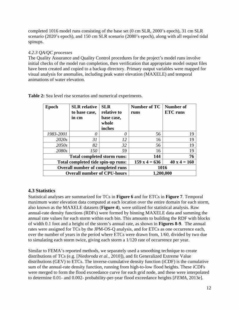
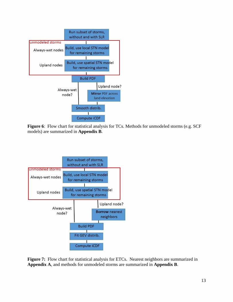
4.3 Statistics Statistical analyses are summarized for TCs in Figure 6 and for ETCs in Figure 7. Temporal maximum water elevation data computed at each location over the entire domain for each storm, also known as the MAXELE datasets (Figure 4), were utilized for statistical analysis. Raw annual-rate density functions (RDFs) were formed by binning MAXELE data and summing the annual rate values for each storm within each bin. This amounts to building the RDF with blocks of width 0.1 foot and a height of the storm’s annual rate, as shown in Figures 8-9. The annual rates were assigned for TCs by the JPM-OS-Q analysis, and for ETCs as one occurrence each, over the number of years in the period where ETCs were drawn from, 1/60, divided by two due to simulating each storm twice, giving each storm a 1/120 rate of occurrence per year. Similar to FEMA’s reported methods, we separately used a smoothing technique to create distributions of TCs (e.g. [Niedoroda et al., 2010]), and fit Generalized Extreme Value distributions (GEV) to ETCs. The inverse-cumulative density function (iCDF) is the cumulative sum of the annual-rate density function, running from high-to-low flood heights. These iCDFs were merged to form the flood exceedance curve for each grid node, and these were interpolated to determine 0.01- and 0.002- probability-per-year flood exceedance heights [FEMA, 2013e].

13

Figure 6: Flow chart for statistical analysis for TCs. Methods for unmodeled storms (e.g. SCF models) are summarized in Appendix B.

Figure 7: Flow chart for statistical analysis for ETCs. Nearest neighbors are summarized in Appendix A, and methods for unmodeled storms are summarized in Appendix B.

14

Figure 8: Tropical cyclone (TC) annual-rate density function for flood height vs annual rate (in thousandths, as signified by x 10-3) at The Battery (1983-2001 epoch). The raw distribution is shown with blue “building blocks”, the smoothed distribution with a red line, and for reference the FEMA 100y and 500y flood heights are shown with vertical dotted lines (at 11.55 and 15.05 feet, before a datum correction of -0.25 feet).

Figure 9: Extra-Tropical cyclone (ETC) annual-rate density function for flood height vs annual rate at The Battery (1983-2001 epoch). The raw distribution is shown with blue “building blocks”, and the distribution is later fitted with a GEV distribution. For reference the FEMA 100y and 500y flood heights are shown with vertical dotted lines.

15

The PDFs for TCs were smoothed with a Gaussian filter [FEMA, 2013e; Niedoroda et al., 2010], using the estimated standard error of 2.2 ft as the filter’s defining standard deviation. This uncertainty was computed as a combination of error arising from simplifications to TC atmospheric fields, and hydrodynamic model error that was quantified with comparisons of historical TC high water marks with model results [FEMA, 2013e]. Extra-Tropical Cyclones (ETCs) were treated with different statistical methods, instead using an assumed Generalized Extreme Value distribution type (GEV) with the L-Moments method for finding the best fit parameters for the distribution (code loaned by URS Corp from the FEMA study). The estimated standard error in ETC flood model results was 0.92 feet, based on hydrodynamic model error that was quantified with comparisons of historical TC high water marks with model results. This is a smaller value than that used for TCs because reanalyses of wind and pressure fields were utilized, instead of simplified parametric TC models. This standard error was similarly used for smoothing before summing to create the iCDFs (flood exceedance curves) [FEMA, 2013e]. 4.3.1. Flood exceedance curves A cumulative sum of each RDF is computed from right-to-left (high-to-low flood height), forming an inverse Cumulative Density Function (iCDF; Figures 10-11). As a consistency check, it was verified that using our statistical methods with FEMA’s ADCIRC modeling outputs (MAXELE files), we closely reproduced FEMA flood exceedance curves for using their MAXELE data (generally within 5cm). The TC and ETC iCDFs were merged into combined iCDFs, also known as flood exceedance curves or stage-frequency curves. These can also be re-plotted by swapping the x and y axes and taking the reciprocal of probability-per-year to obtain the return period, as shown in Figures 12-13. 4.3.2. Flood still water elevations (SWEL) and mapping Estimation of the 100-year and 500-year SWEL values was performed by interpolating the iCDF for each node on the ADCIRC grid to the 0.01 and 0.002 annual exceedance rate. A conversion between the model’s mean sea level and the datum NAVD88 was performed using The Battery 1983-2001 epoch conversion where MAXELENAVD88 = MAXELEMSL - 0.063 m. The actual values of this correction vary by about a centimeter over the NYC region, but the constant value was utilized and the difference of < 1 cm were deemed negligible. The resulting SWEL values were imported into ArcMAP and interpolated (Kriging1 technique) to form a raster surface over the entire region (NYC and the NJ Harbor regions). These values were differenced with the similarly interpolated ADCIRC grid (essentially a coarse-resolution digital elevation model), to compute a map (raster) of flood depth. This flood depth’s zero contour is the boundary of that event’s flood zone.

1 Kriging, or Gaussian process regression, is an interpolation technique where interpolated values are modeled by a Gaussian process governed by prior covariances

16

Figure 10: Inverse Cumulative Density Functions at The Battery (top) and Midland Beach (bottom) for TCs (“Stevens” is hydrodynamic modeling), vs FEMA results with superposition. All exceedance rates for flood heights below ground elevation (dashed line) are set to the sum of all storm frequencies. Before the interpolation and mapping of 0.01 and 0.002 rate events, annual exceedance rates for heights below “ground” level are omitted (“dry” flood heights).

17

Figure 11: Inverse Cumulative Density Functions at The Battery (top) and Midland Beach (bottom) for ETCs (again, “Stevens” is the hydrodynamic modeling results), versus FEMA results with and without superposition of sea level rise.

18

5.0 Results Results for still water flood elevations (SWELs) interpolated from the combined (TC plus ETC) flood distributions (iCDFs) are shown in Table 3. A sample flood exceedance curve for TCs is shown in Figure 12, and is contrasted versus the FEMA baseline sea level curve and curve that represents simple superposition of the FEMA SWELs plus sea level rise. Sample flood exceedance curves for ETCs are similarly contrasted against superposition for two stations in Figure 13. Return period reductions caused by sea level rise are shown in Table 4, with a contrasting of hydrodynamic modeling and superposition results (no bathtubbing was used here, only vertical superposition). A map of the 100-year flood contours for the 1983-2001 epoch versus the 2080s 90th-percentile sea level rise scenario is shown in Figure 14. The raw SWEL dataset or the interpolated raster dataset are both available and can be interpolated onto higher-resolution DEM data, as was done by FEMA. Furthermore, it is expected that the New York City Panel on Climate Change (NPCC) will perform more detailed mapping and include it in its forthcoming report in early 2014. Return period reductions caused by sea level rise are shown in Table 4, with a contrasting of hydrodynamic modeling and superposition results. Table 3: Results for 100-year and 500-year still-water elevation flood heights (NAVD88) with sea level rise, compared with baseline 1983-2001 sea level1

Sea Level Epoch

Sea Level Rise

The Battery,

Manhattan

Willets Point, North

Queens

Belle Harbor,

Rockaway Peninsula

Midland Beach, Staten Island

Howard Beach, South

Queens

(ft) 100y

(ft) 500y (ft)

100y(ft)

500y(ft)

100y (ft)

500y (ft)

100y (ft)

500y (ft)

100y (ft)

500y (ft)

Baseline (1983-2001)

0 11.3 14.8 13.0 14.8 11.1 15.2 11.7 16.0 9.7 12.5

2020s 1.0 12.3 15.7 13.9 15.6 12.0 16.1 12.7 16.8 10.8 13.5

2050s 2.7 13.8 17.3 15.4 17.2 13.6 17.5 15.0 19.3 12.6 15.4

2080s 4.9 15.9 19.4 17.7 19.7 15.5 19.2 16.6 19.6 15.0 17.6

1 The 1983-2001 values are from our statistical analysis and are nearly identical to (within 0.1 ft) to FEMA’s results. However, the NPCC (2013) report lists baseline (1983-2001) values for The Battery that are 0.4-0.5 ft lower (10.8, 14.4 ft). This discrepancy arose because that earlier report utilized a location in Battery Park, whereas here we focus on the exact location of the in-water tide gauge for the purposes of historical comparison and cross-comparisons with other studies.

19

Figure 12: Comparison of TC FEMA flood exceedance curve with 2050s superposition and hydrodynamic mapping (this study) results, for (top) The Battery and (bottom) Midland Beach.

20

Table 4: Flood exceedance values and return periods for hydrodynamic (hydro) and superposition (super) results for floods with 90th-percentile sea level rise.

The Battery  Baseline  2020s  2020s 2050s  2050s  2080s  2080s

super hydro Super Hydro  super  hydro

annual chance of today's 100‐year flood height  1%  1.6 1.7 3.7 3.8  13.2  13.3

annual chance of today's 500‐year flood height  0.20%  0.31 0.31 0.68 0.63  1.9  1.8

future return period of today's 100y flood height  100  61 59 27 26 8  8

future return period of today's 500y flood height  500  318 318 147 158  51  57

Midland Beach  Baseline  2020s 2020s 2050s 2050s  2080s  2080s

  super hydro super Hydro  super  hydro

annual chance of today's 100‐year flood height  1%  1.5 1.7 2.7 4.4 n/a1  16

annual chance of today's 500‐year flood height  0.20%  0.29 0.30 0.55 0.73  1.3  1.6

future return period of today's 100y flood height  100  66 60 37 23 n/a1  6.4

future return period of today's 500y flood height  500  340 333 183 136  76  64

1 No flooding occurs for two of the scenarios at Midland Beach, which is 1.1 km inland

21

Figure 13: Comparison of ETC FEMA flood exceedance curve (black circles) with 2050s superposition (red circles) and 2050s hydrodynamic mapping results (line; this study).

22

Figure 14: Map showing 100-year flood zone for the baseline (1983-2001) epoch, as used by FEMA, and for the 2080s 90th-percentile sea level rise scenario, on top of land surface elevation (feet NAVD88).

6.0 Discussion The comparisons of methods in Figures 12-13 contrast superposition and hydrodynamic-model based results. In the case of The Battery, the TC results show resulting flood elevations that are just below those computed with superposition, and the ETC results show values nearly equal to superposition. For Midland Beach, however, both TC and ETC results show hydrodynamic model flood heights that lie well above superposition. Results across the region are shown in Figure 15, in the form of the ratio of hydrodynamic modeling estimates of the 100-year SWEL to those for “superposition/bathtub”, for 2050s sea level rise. For this comparison, sea level rise was superimposed and then bathtub interpolation

23

extended flood heights over floodplains (nearest-neighbor technique) here. For the tropical cyclone (TC) results, values deviate from 1.00 more often. For the combined storm results (bottom panel) and the ETC results (not shown) more often fall within a few percent of 1.00. This occurs because the ETC assessed flood heights are higher than the TC flood heights, and thus end up controlling the combined assessment. The deviations of hydrodynamic results from the superposition/bathtub approach likely arise due to a combination of frictional effects acting on fast-moving storm tides and due to wind-driven local gradients in sea level. The relative success of superposition/bathtub for ETCs is because both these dynamical effects should be smaller during ETCs than TCs, which have stronger winds and faster-moving water. Midland Beach appears to be a location with anomalous dynamics, with high hydrodynamic-to-superposition/bathtub ratios for both ETCs and TCs. Other areas of Staten Island nearby have lower values near 1.0 for ETCs and the combined assessment. However, the entire eastern shore of Staten Island shows high values above 1.10 for TCs, signifying that superposition/bathtub is not a “conservative” method (risk-averse; erring on the side of a high-bias) of estimating the effect of sea level rise on TC flood heights in this region. The detailed causes of these anomalous dynamics are under further study. The TC results for deepwater and harbor locations generally showed flood elevations that were close to or just below superposition. This result was observed for most TCs at NY Harbor locations like The Battery – a model result for flood height with sea level rise was less than a model result for flood height with superimposed sea level rise. A few physical interpretations are: (1) that as flood levels rise higher with sea level rise, the flood plain cross-section across which the flood travels is expanding, and thus some volume of water is spreading out instead of just rising upward; and (2) this result could be related to tide-surge interactions or simple changes to tide ranges – either mechanism would need to be evaluated further, and other mechanisms may also exist. The difference was weaker for ETCs, however, possibly due to weaker tide-surge interactions due to slower water velocities associated with the (typically) more gradual ETC storm surges. A final consideration is that ADCIRC is a two-dimensional model and neglects stratification, which has been shown to cause underestimation of storm tides [Orton et al., 2012]. Estuary stratification may increase with sea level rise due to the corresponding larger depths and weaker turbulent mixing, and this change is not captured with the ADCIRC modeling. An ancillary benefit of hydrodynamic modeling of flood hazards is the availability of the flood model for adaptation experiments. In the Mayor’s Special Initiative on Rebuilding and Resilience after Sandy, modeling was used to develop a set of coastal adaptation options such as storm surge barriers, breakwaters and wetlands (plaNYC, 2013). The modeling provided quantitative information on the efficacy of these flood adaptations and to iteratively adjust them to correct problems such as backdoor flooding (e.g., around the low-lying area behind Coney Island). Another benefit is the availability of quantitative metrics of flooding such as water velocity, wave heights, or wave orbital velocity, which can be of use for planning purposes. These variables are not available for studies of sea level rise that use only superposition.

24

Figure 15: Maps with shading representing the ratio of hydrodynamic-to-superposition/bathtub results for flood elevations (2050s 90th-percentile sea level rise on 100-year flood). The top panel is from the results for tropical cyclones only, and shows many areas with values above 1.2, signifying hydrodynamic results substantially greater than superposition/bathtub. The bottom panel shows the results from the combined assessment, in which most locations have a value near 1.00. Results for extra-tropical cyclones are also usually near 1.00.

25

6.1 Study limitations The use of a limited set of storms, 25, 65 and 25 for the three subsequent future decades respectively, is well below the total storm set of 219. The uncertainty arising from this methodological simplification is being evaluated by running all 219 storms for the 2050s decade, from which results can be contrasted. Our expectation, however, is that difference will be very subtle – the reason for this is that the physics of flooding is being captured by the current set of methods, and one need not run 219 simulations over four sea level scenarios to simply understand how a water depth change influences flood height. This study relied on the FEMA hazard assessment approach, which was an unprecedented detailed study of the region’s flood hazards, yet had a few limitations. Uncertainties are used for smoothing out RDFs (Figure 8) before summing into iCDFs, and are not available on the final SWEL estimates or annual exceedance rates. An alternative approach would be to fit a distribution to the RDFs as was done for the ETCs and apply the uncertainty to the distribution fitting procedure or as a Monte Carlo analysis. With these alternative approaches, a confidence interval on the distribution could be obtained, which would be more compatible with a holistic approach to flood elevation uncertainty, leaving open the option of merging it with other sources of uncertainty such as that associated with future sea level rise. And put another way, the NPCC sea level rise scenarios are presented as percentile-ranked values, yet there is no straightforward way for similarly assessing the xx-percentile SWEL using the FEMA approach. Another limitation to FEMA’s study is simply one of timing – the storm climatology assessment was completed before Hurricanes Irene and Sandy hit the NYC region and thus, these storms were not available to inform the climatology. This raises the obvious question of how Sandy’s storm track, hybrid storm type, and record-setting storm surge would have affected results. This study does not quantify future changes to wave heights or base flood elevations across the city, but an exploratory analysis of sea level rise effects on wave heights was conducted for a small number of urban transects using the computer wave model that FEMA uses, WHAFIS. A common result around the wave-affected shoreline region (e.g. FEMA V-Zones) was that waves were breaking and were therefore depth-limited as they rolled into the edges of the city. Depth-limited waves typically had a height that was ~60% of the water depth, so an increase in water depth due to sea level rise (SLR) would lead to a 0.6*SLR increase in wave height. As a result, BFEs in these wave-influenced zones will often rise by 1.6 times the sea level rise value. Lastly, the study does not consider changes to the land surface such as reductions in wetland areal coverage or coastal adaptations and protections. Wetland coverage is expected to decrease if wetland substrates do not have sedimentation at a rate sufficient to keep up with sea level rise, and this reduction in friction can lead to increases in storm tides [McKee-Smith et al., 2010]. However, most wetlands have already been lost from the system, and in a separate study using ADCIRC we found that changes to the areal coverage of wetlands in some areas of NYC (e.g., Jamaica Bay) would only have a small effect on storm tides [NYC-EDC, 2013]. Coastal adaptations and protections are difficult to anticipate and are beyond the scope of this study.

26

6.2 Sensitivity analysis: Storm climatology change Storm climatology changes, like sea level changes, can alter return periods for a given flood level [Lin et al., 2012], and recent evidence suggests this may already be occurring due to both regional reductions in aerosol emissions [Villarini and Vecchi, 2012] and atmospheric warming [Grinsted et al., 2013]. Grinsted et al. [2012] found a doubling of “Katrina-level” TCs in years with warm global air temperatures, based on analysis of historical tide gauge data in the US East and Gulf Coasts. A simple sensitivity test was conducted based on this finding, where in the statistical analysis we doubled the annual rates of TCs. The results are shown in Table 5, and show that effects on the 100-year and 500-year flood for The Battery were 0.6-0.7 ft increase, and for Willets Point (reflecting the eastern end of East River and Western Long Island Sound) were smaller, 0.2-0.3 ft.

Table 5: Increase in still water elevations resulting from a hypothetical doubling of TCs

Sea Level Epoch The Battery Willets Point

100y (ft) 500y (ft) 100y (ft) 500y (ft)

Baseline (1983-2001)

0.7 0.6 0.2 0.3

2020s 0.6 0.6 0.3 0.4

2050s 0.6 0.5 0.2 0.3

2080s 0.6 0.5 0.3 0.3

6.3 Comparison of these results to prior studies This flood assessment effort for New York City includes the surrounding parts of New Jersey around New York Harbor, which is a crucial part of New York City’s transportation, energy and food distribution system. Prior efforts from the NPCC only focused within the city’s borders. This study relies upon methods used for FEMA’s base hazard assessment, which finds higher regional estimates of 100-year and 500-year storm tides than those of other studies or data analyses. Generalized Extreme Value distribution fits of observed storm tides at The Battery tide gauge provide an observation-based alternative estimate for 100-year storm tide of 7.86 ft NAVD88 (http://tidesandcurrents.noaa.gov/est), as compared with the FEMA estimate of 11.3 ft, a difference of nearly 3.5 ft. Prior to this new study, FEMA’s storm tides for 100-year floods was estimated to be 8.6 ft NAVD88 [Horton et al., 2010]. Also, a study of only TC storm tides [Lin et al., 2012] concluded that the 100-year TC storm tide is 6.45 ft NAVD88 (2.03 m MSL), compared with FEMA’s 100-year TC storm tide of 9.02 ft. Discrepancies for 500-year storm tides are similarly large.

27

6.4 Future research needs The FEMA study found that the hazard assessment for New York Harbor (The Battery) – elevations of 100- and 500-year storm tides – are controlled predominantly by the extra-tropical cyclones. This result contradicts the fact that three of the six highest flood events since 1927 (the available hourly tide gauge record) were tropical cyclones, and furthermore, newspaper accounts and recent paleo-tempestology research suggests three hurricanes in prior centuries were the highest historical flood events [Scileppi and Donnelly, 2007], just below Sandy. Granted, the FEMA study’s historical assessment was completed in 2010, prior to two of these storms (Irene and Sandy), so at that time only one of the six highest storm tides in the tide gauge period was caused by a TC. It is also noteworthy that the largest storm surge in the historical record of 1927-2009 was an extra-tropical storm on November 25, 1950, at 7.6 ft. However, that storm surge peaked at the time of low tide, and the peak storm tide was lower than several other flood heights on record. The relative importance of ETCs and TCs for defining the region’s flood hazard are an important topic for further analysis. As stated in Section 6.1, it would be valuable to develop and utilize a hazard assessment framework that has a holistic approach to flood elevation uncertainty, merging the hazard assessment sources of uncertainty with uncertainty for future sea level rise and storm climatology changes.

Acknowledgements This research was supported by the City of New York. This research was also supported, in part, by a grant of computer time from the City University of New York High Performance Computing Center under NSF Grants CNS-0855217, CNS-0958379 and ACI-1126113. Special thanks to Hugh Roberts, Zach Cobell, Casey Dietrich, Alan Niederoda, Asher Taylor, Chris Reed, Gabriel Toro, Paul Muzio, Andrew Martin, Chris Little, Ning Lin, Yochanan Kushnir, Klaus Jacob, Vivien Gornitz, Radley Horton, Cynthia Rosenzweig, Dan Bader, Leah Cohen, Carrie Grassi, and others at their respective organizations.

References FEMA (2013a), Redefinition of the Coastal Flood Hazard Zones in FEMA Region II: Analysis of the Coastal 

Storm Surge Flood Frequencies, Fairfax, VA. FEMA (2013b), Final Draft Report: Region II Storm Surge Project Mesh Development Report, prepared by 

Risk Assessment, Mapping, and Planning Partners (RAMPP), Washington, DC. FEMA (2013c), Region II Storm Surge Model Calibration and Validation Report, Prepared by Risk 

Assessment, Mapping, and Planning Partners (RAMPP), Washington, DC. FEMA (2013d), Revised Final Draft: Production runs for the FEMA Region 2 New York/New Jersey Surge 

Modeling, Risk Assessment Mapping and Planning Partners (RAMPP), Washington, DC. FEMA (2013e), RECURRENCE INTERVAL ANALYSIS OF COASTAL STORM SURGE LEVELS AND WAVE 

CHARACTERISTICS FOR THE NEW YORK/NEW JERSEY COASTAL SURGE STUDY, Risk Assessment, Mapping and Planning Partners (RAMPP), Washington, DC. 

28

Gallien, T., J. Schubert, and B. Sanders (2011), Predicting tidal flooding of urbanized embayments: A modeling framework and data requirements, Coastal Engineering, 58(6), 567‐577. 

Gesch, D. B. (2009), Analysis of lidar elevation data for improved identification and delineation of lands vulnerable to sea‐level rise, Journal of Coastal Research, 49‐58. 

Grinsted, A., J. C. Moore, and S. Jevrejeva (2012), Homogeneous record of Atlantic hurricane surge threat since 1923, Proceedings of the National Academy of Sciences, 109(48), 19601‐19605. 

Grinsted, A., J. C. Moore, and S. Jevrejeva (2013), Projected Atlantic hurricane surge threat from rising temperatures, Proceedings of the National Academy of Sciences, 110(14), 5369‐5373. 

Horton, R., V. Gornitz, M. Bowman, and R. Blake (2010), Chapter 3: Climate observations and projections, Annals of the New York Academy of Sciences, 1196(1), 41‐62, DOI: 10.1111/j.1749‐6632.2009.05314.x. 

Lin, N., K. Emanuel, M. Oppenheimer, and E. Vanmarcke (2012), Physically based assessment of hurricane surge threat under climate change, Nature Climate Change. 

McKee‐Smith, J., M. A. Cialone, T. V. Wamsley, and T. O. McAlpin (2010), Potential impact of sea level rise on coastal surges in southeast Louisiana, Ocean Engineering, 37(1), 37‐47. 

Niedoroda, A., D. Resio, G. Toro, D. Divoky, H. Das, and C. Reed (2010), Analysis of the coastal Mississippi storm surge hazard, Ocean Engineering, 37(1), 82‐90. 

NPCC (2013), CLIMATE RISK INFORMATION 2013: Climate Change Scenarios and Maps, New York City Panel on Climate Change. 

NPCC (2014), Climate Risk Information 2014, New York City Panel on Climate Change. NYC‐EDC (2013), Chapter 3: Coastal Adaptation, in NYC Special Initiative on Rebuilding and Resilience, 

edited by D. Zarrilli, New York City Economic Development Corporation. Orton, P., N. Georgas, A. Blumberg, and J. Pullen (2012), Detailed Modeling of Recent Severe Storm 

Tides in Estuaries of the New York City Region, J. Geophys. Res., 117, C09030, DOI: 10.1029/2012JC008220. 

Orton, P., S. Vinogradov, N. Georgas, and A. Blumberg (2013), Hydrodynamic Mapping of Future Coastal Flood Hazards for New York City, 27 pp, Final report prepared for New York City Office of Emergency Management. 

Rosenzweig, C., et al. (2011), Developing coastal adaptation to climate change in the New York City infrastructure‐shed: process, approach, tools, and strategies, Climatic Change, 1‐35. 

Scileppi, E., and J. P. Donnelly (2007), Sedimentary evidence of hurricane strikes in western Long Island, New York, Geochemistry, Geophysics, Geosystems, 8(6), DOI: 10.1029/2006GC001463. 

Stamey, B., H. Wang, and M. Koterba (2007), Predicting the next storm surge flood, Sea Technol., 48(8), 10. 

Titus, J. G., and C. Richman (2001), Maps of lands vulnerable to sea level rise: modeled elevations along the US Atlantic and Gulf coasts, Climate Research, 18(3), 205‐228. 

Toro, G., A. Niedoroda, C. Reed, and D. Divoky (2010), Quadrature‐based approach for the efficient evaluation of surge hazard, Ocean Engineering, 37(1), 114‐124. 

Villarini, G., and G. A. Vecchi (2012), Twenty‐first‐century projections of North Atlantic tropical storms from CMIP5 models, Nature Climate Change, 2(8), 604‐607. 

Westerink, J., R. Luettich, and J. Muccino (1994), Modelling tides in the western North Atlantic using unstructured graded grids, Tellus A, 46(2), 178‐199. 

Zhang, K., Y. Li, H. Liu, H. Xu, and J. Shen (2013), Comparison of three methods for estimating the sea level rise effect on storm surge flooding, Climatic Change, 1‐14. 

29

APPENDIX A: Upland nodes – using the FEMA study approach The process of building annual-rate density functions (RDFs) for upland areas above mean sea level for TCs and ETCs, different methods were utilized to account for non-flooding storms. The problem arises that non-flooding storms are useful for building a RDF of height, even if their height above ground is effectively negative. In seeking to reproduce the methods utilized in the FEMA Region II flood mapping study, we attempted to reproduce their methods for doing this as closely as possible, and these are summarized here. For TCs, we used reflection across ground elevation to extend our RDFs. This has an effect on flood heights in the smoothed RDF due to the Gaussian smoothing (Figure A1). The FEMA study utilized offshore node data to fill out RDFs of flood height for “dry storms” in their ETC statistical analysis, as do we for our study. This is simply bathtubbing, from a set of pre-computed set offshore nearest neighbors. Figure A2 shows lines connecting upland-offshore node pairs, which were created for all grid nodes that are located at land elevations above -1.5 m (1.5 m below the baseline mean sea level). A diagram demonstrating the purpose of borrowing offshore node data is shown in Figure A3. These “borrowed” flood heights are below ground at the upland node of interest, but help build a more complete RDF that can be fit with the GEV distribution, improving the stability of the statistical analysis – consider a case where only a few storms actually flood an upland node. If a GEV distribution must be fit to the two-point RDF, then it has very high uncertainty. Borrowing 58 more flood heights for the lower part of the distribution provides a much more stable fit for the distribution.

Figure A1: TC annual-rate density function showing reflection across ground level (4.1 feet NAVD88).

30

Figure A2: Map of Lower Manhattan showing lines connecting upland-offshore node pairs. The FEMA study utilized offshore node data to fill out RDFs of flood height for “dry storms” in their ETC statistical analysis, as do we for our study.

31

Figure A3: Schematic diagram of an upland node and a nearest offshore (“wet”) node. In this sample case, four storms flood the upland node, whereas 9 storms flood the offshore node. The 1% surge level floods the upland node, yet building statistics for that node based on only a 4-point RDF is sub-optimal. Note that using offshore nodes assumes flood heights are the same at both locations. Figure courtesy of Chris Reed, URS Corp.

32

APPENDIX B: Unmodeled storms This study utilized a limited set of storms, 75, 35, 75 and 35 for the baseline, 2020s, 2050s and 2080s sea level scenarios. In total this was 25% of the total storm set of 219, but was a requirement and agreed upon in advance with the program manager because the time period of the study was only several months and 219 x 4 model runs would take too long even on the supercomputing system that was used. In performing this number of model runs alone, about 1.2 million CPU-hours were used, the equivalent of running a four-processor computer for 34 years.

B.1. Storm subsetting Many of the modeled storms in FEMA’s set do not cause over-land flooding in the NYC region, and the non-flooding storms are therefore less valuable for the hazard assessment in this area. Taking advantage of this factor, a subset was objectively determined that covers (1) all the storms that caused substantial over-land flooding, indicative of 100-year and 500-year events, and (2) a smaller number of storms that spans the full range of flood heights around NYC. Three locations in the NYC region were chosen to help guide these objective determinations, representative of different flooding sub-regions (Figure 4) – The Battery (NY Harbor), Willets Point (upper East River) and Belle Harbor (the open ocean shoreline). “Substantial over-land flooding” was defined as a flood height more than 1.5 ft above seawall heights at any of these three locations, as model results showed that very little land area flooded for flood heights below this level. A summary of error analyses that address the added uncertainty caused by this subsetting of storms is included below, in Section B.2. Differences caused by the reduced set of modeled storms are subtle – the reason for this is that the physics of flooding is being captured by the hydrodynamic model runs, and one need not run 219 simulations over four sea level scenarios to simply understand how a water depth change influences flood height.

33

Figure B1: Two sample cases of MAXELE data that highlight spatial gradients in flood elevation, with a (left) severe tropical cyclone (storm NJb_0001_007) and a (right) severe extratropical cyclone (the December 1992 nor’easter). The wind direction at the time of peak water elevations for the TC was southeast, and for the nor’easter was east-northeast, highlighting a typical difference between these types of storms. On the left figure, two locations are noted – a location 1.1 km inland at Midland Beach, and a location several kilometers inland through tidal channels and wetlands in Fresh Kills. Note the different color scales for each panel. The methods used for synthesizing un-modeled storms included use of local “Superposition Correction Function” (SCF) to fill in MAXELE data for offshore nodes, and “Bathtub Correction Function” (BCF) for upland nodes. In both cases, regression models were built as a function of water depth, because this was observed to be a strong relationship. The physical reasoning for water depth being important to flood height nonlinearity is because the most basic models of water velocity relate it to flow depth (h) – in one case, velocity (U) goes as the square root of gravity times h (shallow-water wave speed). In another simple model, U goes as the log of h (the law of the wall). In both cases, the sensitivity of U to h is highest for small z, and thus non-linearity of the flood velocity is highest. [name – not storm tide nonlinearity] and its relationship with depth were recently studied for Hurricane Andrew flooding around Miami [Zhang et al., 2013]. In that study, it was also observed that nonlinearity was strongest for shallow flood depths. They found that the nonlinearity at the wave-affected open shorefront was negative, whereas for upland areas it was positive. Here, we find similar spatial variations. Nonlinearity is defined herein as the hydrodynamic model flood elevation minus the superposition flood elevation, and is specific to a given sea level rise scenario (not general to all sea level rise scenarios). The functional approach for synthesizing a storm’s MAXELE data at a given location is: MAXELESLR=0.82m = MAXELESLR=0 + 0.82 + SCF(h)

34

Here, SCF(h) is the regression function of SCF versus flow depth (h), and h is the flow depth with no sea level rise. An example of SCF and a regression with flow depth is shown in Figure B1 for The Battery. Two physical interpretations for the reason why SCF is increasingly negative with increasing flow depth are (1) that as flood levels rise higher with sea level rise, the flood plain cross-section across which the flood travels is expanding, and thus some volume of water is spreading out instead of rising upward; and (2) this result could be related to tide-surge interactions or simple changes to tide ranges – either mechanism would need to be evaluated further, and other mechanisms may also exist.

Figure B2: Superposition Correction Function (SCF) results (also known as “storm tide nonlinearity”) at The Battery tide gauge (an offshore model node) for 55 hydrodynamic model storms, with dashed line regression model. Second-degree polynomial regression coefficients are also shown. Deep water sites often have a useful SCF relationship with flow depth, and these regression relationships of SCF with flow depth were applied to offshore “always-wet” nodes for un-modeled storms. However, it is problematic to apply SCF with upland nodes due to the lack of hydrodynamic model data for dry cases where no flooding occurred. As a result, a new approach was utilized.

H = flow depth = MAXELE ‐ land elevation

35

The “Bathtub Correction Function” (BCF) relates to the bathtubbing technique where flood heights are expanded spatially, and is a correction to that technique that is based on hydrodynamic modeling results. This approach was used to synthesize flood heights for upland nodes in the assessment. It is defined as the upland node MAXELE minus the offshore node MAXELE, both from hydrodynamic modeling results. Similar to the SCF approach, a regression relationship of BCF with bathtubbed (projected) flow depth (hprojected) is applied to upland nodes for un-modeled storms: MAXELEupland = MAXELEoffshore + BCF(hprojected) A sample result for a BCF regression is shown in Figure B2 for Hoboken, NJ.

Figure B3: Bathtub Correction Function (BCF) (also known as “spatial storm tide nonlinearity”) based on hydrodynamic model results (+) and second-degree polynomial best-fit (dashed lines) to the data. A regression model for each model node is fitted and then used for synthesizing un-modeled storms, along with the SCF regression models.

A different plotting perspective on BCF is shown in Figure B3, as well as a spatial map of MAXELE for one storm that shows how these regressions relate to actual flooding spatial patterns. A wind velocity vector representing the winds in the hour prior to the period of peak water elevation is also shown that demonstrates the physical reasons likely responsible for the

“bathtubbed water depth”

36

spatial patterns. The example shows how a SE wind (blowing towards the NW) can cause the observed pattern where flood heights are spatially varying due to winds. Flood heights at Midland are higher than the offshore node, whereas flood heights at Fresh Kills are lower than at the offshore node, due either to only wind or potentially also the large amount of friction in the wetlands in that region that can prevent water from penetrating so far eastward.

A more detailed analysis of BCF and SCF could examine the importance of wind direction, but this was beyond the scope of this study and would require analyzing a substantial amount of additional meteorological data.

B.2 Error assessment for modeling only a subset of storms For the present-day and 2050s TC assessments, 35% of storms (56) were included in the modeling subsets, and the assessment utilized synthesized MAXELE data for the remainder of the storms. In contrast, only 10% of the storms were included in the subsets for the 2020s and 2080s (16). The two periods for which a larger set were used as a test of sensitivity to using the smaller subsets. The results for the 100y and 500y SWEL for 56 storms was very similar to the results using 16 storms – deepwater sites (e.g. The Battery) averaged a difference of 0.01 ft across the city, whereas upland sites (e.g. Midland Beach) averaged a difference of 0.1 ft. The contribution of these differences to the total flood hazard were even smaller.