identiﬁcation of rational speculative bubbles in ibovespa...

Identification of Rational Speculative

Bubbles in IBOVESPA (after the

Real Plan) using Markov Switching

Regimes

Diogenes Manoel Leiva Martin,

Eduardo Kazuo Kayo,Herbert Kimura, Wilson Toshiro Nakamura

Mackenzie Presbyterian University, Sao Paulo, Brazil

AbstractThe present article aims to verify the presence of rational specula-

tive bubbles by identifying the regime switching of the return gener-ating process in the Brazilian stock exchange market, BOVESPA, forthe Real Plan period (July 1994 to March 2004). To achieve this goal,a Markov switching regime was used, and then the nonlinear structureof data was verified in relation to conditional mean and variance. Asa result, the dynamics of the data generating process can be describedas a function of two regimes (bull markets and bear markets). Thesecycles, however, were decomposed into other cycles, initial and finalphases of the cycles of growth (bull) and decrease (bear). This decom-position proved more coherent with the concept of speculative bubble,in which there is a nonlinear relationship between stock prices andtheir fundamentals.

Keywords: Rational Speculative Bubble, Markov SwitchingRegimes, Nonlinearities, Market Efficiency

Revista EconomiA December 2004

Diogenes Martin, Eduardo Kayo, Herbert Kimura e Wilson Nakamura

Classificacao JEL: G14, C39, C52

O presente artigo procurou constatar a presenca de bolhas es-peculativas racionais, a partir da identificacao de mudanca deregime do processo de geracao de retornos no mercado brasileirode acoes na BOVESPA, para o perıodo pos Plano Real (julhode 1994 a marco de 2004). Para tentar lograr este fim, utilizou-se do modelo de regimes de conversao markovianos, que per-mite identificar a estrutura nao linear dos dados seja em relacaoa media condicional, seja em relacao a variancia condicional.Como resultado a dinamica do processo de geracao dos retornospode ser descrito como funcao de dois regimes (“bull markets”e “bear markets”). Estes ciclos, porem, puderam ser decompos-tos em outros ciclos, fases iniciais e finais do ciclo de cresci-mento (“bull”) e de crescimento (“bear”). Esta decomposicaomostrou-se mais coerente com o conceito de bolha especulativa,no qual ha uma relacao nao linear entre o preco das acoes e osseus fundamentos.

1 Introduction

The returns generating process, as pointed out by French (1980),has been the most widely investigated topic in finances and orig-inated from the publication of Bachelier’s thesis in 1900. There-fore, the origin of the Finance Theory is tangled up with this

⋆ Email addresses:[email protected] (Diogenes Manoel Leiva Martin),[email protected] (Eduardo Kazuo Kayo),[email protected] (Herbert Kimura),[email protected] (Wilson Toshiro Nakamura).

216 EconomiA, Selecta, Brasılia(DF), v.5, n.3, p.215–245, Dec. 2004

Identification of Rational Speculative Bubbles in IBOVESPA (after the Real Plan)

concern with market efficiency.

Tobin (1984) apud Barone (1990) describes the classification thatestablishes four types of efficiency: 1) efficiency in terms of in-formation; 2) efficiency regarding the number of assets, that is,the market must be complete; 3) efficiency in terms of opera-tion and; 4) efficiency in terms of evaluation, that is, the stockprices reflect or should reflect the present value of their futureearnings (dividends). In this regard, the stock price should havean intrinsic value.

According to Jensen (1978), any market strategy that consis-tently produces economic gain, after discounting the risk, for asufficiently long period, considering the transactions costs, is apiece of evidence against market efficiency. This concept is suffi-ciently general to incorporate the above-mentioned Tobin’s tax-onomy. Traditionally, the concern of researchers with efficiencycan be translated as the hypothesis that the natural logarithmof stock prices behaves as a martingale difference in relation tofiltration. This is the same as to say that the value expected fromthe excess rate of return is on average equal to zero, consid-ering a measure of probability that discounts the risk premium,given a set of (historical, public or private) information.

Empirical evidence, especially from the 1960s, has overwhelm-ingly demonstrated an array of stylized facts, which gave riseto a vast literature on finances, such as: volatility clusters, non-normality of returns, negative asymmetry, excess kurtosis,stochastic volatility, autoregressivity of returns and volatility,market anomalies related to seasonality or to the operation ofthe market, market anomalies related to the size of the firm andits capital structure, mean-reverting process for returns and ex-treme values. Concomitantly with these findings, a series of the-ories (mainly economic ones) were posited on the nonlinearity ofdata, including fads, manias and panics and rational speculative

EconomiA, Selecta, Brasılia(DF), v.5, n.3, p.215–245, Dec. 2004 217


bubbles.

The aim of the present study is to verify the presence of rationalbubbles by detecting the regime switching of the returns gener-ating process in the Brazilian stock market (BOVESPA), for theperiod following the Real Plan (July 1994 to March 2004). Theuse of the Markov switching model allows identifying the nonlin-ear structure of data either in relation to the conditional meanor to the conditional variance. As a result, the dynamics of thegenerating process may be a function of bull markets and bearmarkets. These markets may be decomposed into other cycles,such as initial and final stages of the bull and bear markets.

2 Bibliographic Review

2.1 Rational speculative bubble

The most direct empirical evidence is that which considers apersistent rise in asset prices for a sufficiently long period (rally)as a bubble, followed by a collapse in prices (crash). The conceptof bubble can have different meanings. By considering the no-arbitrage and equilibrium arguments, the present value of anasset must equal the value expected from the flow of net benefitsthat this asset generates to its holders. However, in case of astock, the observed value can be higher than the present valueof its dividends. For some reason, the demand exceeds the supplyof that good, causing its price to rise, for a certain period of time,supposing the nonexistence of a monetary phenomenon (inflationor hyperinflation). The origin and nature of this process thatgenerates price movement will characterize the different types ofbubble. In this study, we will deal with the rational speculative



bubble, after regime switching takes place.

The original rational speculative bubble model was developed byBlanchard (1979) and Blanchard and Watson (1982). Accord-ing to this model, the bubble appears when an asset price isan increasing and positive function of the expected future pricemovement. The assumption is that economic agents, under theconditions of forming their price expectations in a rational man-ner, do not commit errors in a systematic fashion and, therefore,the positive relationship between the current price and its futurevariation results in an equally positive relationship between itscurrent price and its observed variation. Thus, the agents’ expec-tations are self-fulfilling, causing the variation in price to drivethe current price towards its expectation, regardless of its funda-mentals. For a given period of time, economic agents follow thisline of thought or belief and this causes prices to rise, regardlessof the flow of dividends. Agents are aware of the possibility of abubble burst, but the expected return makes it worthwhile tak-ing on such risk. However, what is observed is that this deviationbetween the observed price and its intrinsic value can be so largethat one may think of speculation. Hence the origin of the termrational speculative bubble.

Irrational decision-making models such as those proposed byTversky and Kahneman (1981) may explain the speculative na-ture of markets. However, in the speculative bubble model, therationality of agents is preserved and there is a representative in-vestor. A broader concept of bubble encompasses the fads modelproposed by Summers (1986), manias and panics proposed byKindleberger (1989), speculative bubble by Blanchard and Wat-son (1982) and random speculative bubble by Weil (1987). InSummers’ model (1986) there are two types of representativeagents: agents that demand the asset in function of the expectedfuture return and those who demand the asset in function of past



returns. The latter aggregate noise to the market and can act ac-cording to “irrational” negotiation rules, reacting excessively tothe latest news, with information asymmetry or necessitating ahigh cost to obtain them, acting in function of the estimatedbehavior of others. In Kindleberger’s model (1989), collapse ismore likely, the more distant the observed price and the intrin-sic value of the asset, thus placing emphasis on its speculativenature. The model devised by Blanchard and Watson (1982)takes for granted that the bubble has a deterministic behavior,whereas that of Weil (1987) assumes its random nature. Bothhave a rational representative agent who admits the possibilityof sale at a higher price, regardless of the flow of the fundamen-tal asset value. However, as shown by Van-Norden andSchaller (1996), all these models lead to regime switch-ing. Bubbles survive and collapse and, therefore, the generationof returns is associated with the presence of bubbles or with theircollapse. Moreover, the probability of bubble collapse dependson bubble size, i.e., the larger its size, the larger the probabilityof collapse. Thus, the dynamics of bubbles naturally results inregime switching.

Nevertheless, the following aspect should be highlighted: regimeswitching can be a sign that bubbles are present. The behaviorof stock prices, in case of the speculative bubble model, is relatedto the expected flow of dividends. In the fundamental model pro-posed by Van-Norden and Schaller (1996), stock price is relatedto macroeconomic fundamentals. Thus, regime switching mayoccur due to the change in macroeconomic fundamentals or not.In the latter case, the existence of a regime occurs independentlyof the presence of fundamentals that justify it, either becauseprices are being influenced by pieces of news that do not havean impact on the fundamentals, or because prices are relatedto their fundamentals in a nonlinear fashion. Also noteworthy isthat the relationship between macroeconomic fundamentals and



the expected dividends is not necessarily synchronized. Evidenceof this is that decreases in stock prices do not necessarily occurwhen there is a drastic change in macroeconomic fundamentals.The review of the flow of dividends considers a longer-term per-spective, whereas macroeconomic fundamentals consider govern-ment policies in a shorter period of time.

Initially, the tests for detection of bubbles aimed to spot any typeof bubble, without specifying its nature, being therefore moregeneral. To cite a few: Leroy and Porter (1981), Shiller (1981),Mankiw et al. (1985), Mattey and Meese (1986) and West (1987).Basically, these tests focused on defining limits to the varianceby considering the observed asset prices and the present value oftheir dividends.

Later on, other authors tested for bubbles, considering theirspecificity and therefore providing more details about them. Thisis the case of Turner et al. (1989), who assessed the model inwhich the variance of excess return is a function of the stateof the regime, using monthly data from 1946 to 1987, with theS&P500 composite index. Their results showed that the meanreturns were inversely proportional to the level of risk of eachstate, indicating that moments of high volatility took agents bysurprise.

Van-Norden and Schaller (1993) analyzed the predictability ofregime switching in the Toronto Stock Exchange between 1956and 1989. Their results confirmed the evidence that growthbursts that precede collapse result from the deviation from fun-damentals, as suggested by the bubble model. Mcqueen andThorley (1994) found evidence that the probability of a changein the continuously high and persistent stock prices of the NewYork Stock Exchange from 1927 to 1991, on a monthly basis, de-creases in function of the length of this period (negative “hazard”function).



Van-Norden and Schaller (1996) used monthly data on priceand dividends for the U.S. market in the period between 1926and 1989 but did not find any evidence that the predictabil-ity of returns followed a nonlinear relationship. Additionally, thepieces of evidence confirmed that the higher stock prices dur-ing the growth period, the higher the probability of collapse,and that there exists a significant difference between returnsin both regimes (rally and crash). By using monthly data forthe U.S. stock market between 1926 and 1989, Van-Norden andSchaller (1997) proved that the fad and bubble models implyregime switching.

Maheu and Mccurdy (2000) found evidence of nonlinearity ofthe New York Stock Exchange monthly returns for the 1834-1995 period. The authors considered that the largest return oc-curred in periods of economic growth (bull market) and that thesmallest return took place in a period of decrease (bear market).The period with the largest growth corresponded to lower con-ditional volatility and the period with smaller growth was thatwith higher conditional volatility.

Coe (2002) employed the Markov switching regime to investi-gate financial crises, especially the Great Depression in 1929.Evidence suggests that the crisis did not begin with the crash ofthe New York Stock Exchange, but with the bank crisis that fol-lowed it, and that the changes in regulatory milestones triggeredthe regime switching.

Brooks and Karasaris (2003) considered the Markov switchingregime to have three stages: dormant bubble state, explosive bub-ble state and collapsing bubble state. Through monthly data,they analyzed the 1888-2001 period and found that abnormalvolume is a significant predictor of bubble collapse.

In Brazil, Laurini and Portugal (2002) used the Markov switch-



ing regime to validate the hypothesis of market efficiency in rela-tion to the nominal exchange rate (R$/US$). They analyzed thepost-Real Plan until January 2002, using daily data, and vali-dated the hypothesis of efficiency. However, the model identifiedperiods with abnormal gains. Terra and Valadares (2003) alsoused the Markov switching model to verify the alignment or non-alignment of the real exchange rate in a sample of 85 countries.They found two regimes (calmness and crisis) for some countriesand a higher persistence for those which showed a lower rateof appreciation. Valls-Pereira et al. (2004) applied the Markovswitching regime to the stochastic volatility model, in order toanalyze the level of persistence and the dynamics of the volatilityprocess for indices (S&P500 and FTSE100) of the U.S. marketon a daily and weekly basis. Disregarding the presence of regimesgoverning volatility resulted in higher persistence.

2.1.1 General rational speculative bubble model

The bubble model below follows the pattern described by Mc-queen and Thorley (1994). In efficient markets, the value ex-pected from the future return should be the same as the observedvalue. This implies that, in a two-period model, the observed re-turn should be the same as the present value of the dividendand of price variation in the period. Considering an infinite timehorizon, respecting the transversality condition, the fundamen-tal asset price (p∗) should be the present value of the cash flowgenerated by it, represented by the flow of dividends. Thus, thefundamental asset value is also a solution to the first equation.

Et [Rt+1 − r|Ωt] = 0 (1)

Rt+1 = [pt+1 − pt + dt+1] /pt (2)

pt = Et [pt+1 + dt+1] / (1 + rt+1) (3)



p∗ =∞∑

i=1

Et [dt+1]∏i

j=1 (1 + ri+j)(4)

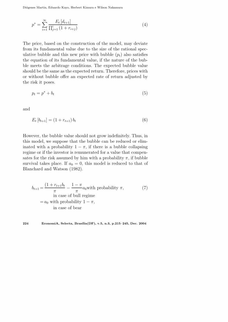
The price, based on the construction of the model, may deviatefrom its fundamental value due to the size of the rational spec-ulative bubble and this new price with bubble (pt) also satisfiesthe equation of its fundamental value, if the nature of the bub-ble meets the arbitrage conditions. The expected bubble valueshould be the same as the expected return. Therefore, prices withor without bubble offer an expected rate of return adjusted bythe risk it poses.

pt = p∗ + bt (5)

and

Et [bt+1] = (1 + rt+1) bt (6)

However, the bubble value should not grow indefinitely. Thus, inthis model, we suppose that the bubble can be reduced or elim-inated with a probability 1 − π, if there is a bubble collapsingregime or if the investor is remunerated for a value that compen-sates for the risk assumed by him with a probability π, if bubblesurvival takes place. If a0 = 0, this model is reduced to that ofBlanchard and Watson (1982).

bt+1 =(1 + rt+1bt

π− 1 − π

πa0with probability π, (7)

in case of bull regime

= a0 with probability 1 − π,

in case of bear



The unexpected variation in prices (εt) has two sources of un-certainty: the unexpected variation of fundamental price (δt+1)and the unexpected variation of the rational speculative bubble(ηt+1). To eliminate the possibility of arbitrage, the unexpectedmean variation (innovation) should be equal to zero. However,innovation can be positive asymmetric in case of price rises ornegative in case of bubble collapse, producing autocorrelationfor returns. Excess kurtosis can be produced by mixing the dis-tributions of probabilities of both regimes. The observations re-sponsible for a smaller variance, compared to the total varianceof observations, will produce more kurtosis and the observationsresponsible for a higher variance, compared to the total variance,will produce fatter tails.

δt+1 = p∗t+1 + dt+1 − (1 + rt+1) p∗t (8)

ηt+1 = bt+1 − (1 + rt+1) .bt (9)

εt+1 = δt+1 + ηt+1 (10)

εt+1 = δt+1 +1 − π

π[(1 + rt+1) .bt − a0] with probability π

= δt+1 + [(1 + rt+1) .bt + a0] with probability 1 − π

(11)

As corollary of the speculative bubble model we have regimeswitching. Nevertheless, regime switching may result from thepresence of speculative bubble and also from the changes in fun-damentals, mainly macroeconomic ones (interest rate, exchangerate, inflation rate, wage levels). Thus, the evidence of bubblefrom the regime switching in this study follows a Markov switch-ing regime.



2.2 Markov switching regimes

Large fluctuations were observed when we analyzed the behaviorof IBOVESPA in the study period. So, the assumption is thatthe nature of fluctuations results from the presence of rationalspeculative bubbles, which imply regime switching. The percep-tion of agents is that there are more or less risky moments toinvest in stock exchanges.

Ryden et al. (1998) proved that a series of stylized facts derivesfrom a Markov switching regime model. Thus, the presence ofthese stylized facts implies evidence of bubble, in which each ofthe different phases follows different regimes.

The concept of nonlinearity refers to the change in regime orstates, that is, certain properties of the time series, such as mean,variance and autocovariance function are remarkably differentdue to distinct regimes. Each of the regimes generates a series ofobservations that can be described by a linear process. However,the combination or sum of these processes generates a nonlineardynamics. The process of transition from one state to anotherfollows a Markov process. In this study, we adopt the modeldeveloped by Hamilton (1989), which is briefly described next.

Let a data generating process (returns) be such that it obeys thefollowing equation:

Rt =µ(St) +p

∑

i=1

φi [Rt−i − µ (St−i)] + σ(St)vt

se St = estado j ∈ (1...M) , where (12)

Rt = 1n(Pt/Pt−1); P is the number os lags or order of the re-gression process; µ(St) is the conditional mean, given the his-



tory of the process Ωt−1 = (St−1, St−2, ..., S1, S0, S−τ+1) and τ =length in each regime, νt is the standard normal innovation (νt ∼NID(0, 1)) which is not dependent upon St and Rt.

For each observation of the return, its expected value, at a givenmoment, given the history of the (Ωt) and the regime (St), as-sumes the following value:

E [Rt|Ωt−1, St] = µ(St) +p

∑

i=1

φi [Rt−i − µ (St−i)] (13)

The difference between the observed value and its expected valueis a martingale difference that follows a standard normal distri-bution with mean zero and whose variance-covariance matrix

∑

depends on regime St.

µt = Rt − E [Rt|Ωt−1, St] ∼ NID(

0,∑

St

)

(14)

However, the generating process above the returns is insufficientto elucidate the dynamics of the process, as the regime switching,due to the construction of the model, follows a Markov process.This process is characterized by a Markov chain that assumesdiscrete states (e.g.: bull or bear markets), as follows:

P =(

p11 1 − p22

1 − p11 p22

)

where pij is the probability to go to state j, since this is state i.

The density probability function conditional on regime St andthe history of the process Ωt−1 follows a normal distribution,



given by:

f (Rt|St = j, Ωt−1, θ) =1√2πσ

exp

−(

Rt − φ′

jxt

)2

2σ2

(15)

where xt = (1, Rt−1, ..., Rt−p)′ and φj = (φ0,j, φ1,j, ..., φp,j)

′, j = 1or 2 and θ = (µ(St = 1), µ(St = 2), p11, p22, σ

2).

The parameters of vector θ are estimated based on the informa-tion contained in Ωt−1. The maximum likelihood function for thenth observation is given by:

L(θ) = 1n[f(Rt|Ωt−1, θ)] = 1n[f(Rt|St = 1, Ωt−1, θ)]

+ f(Rt|St = 2, Ωt−1, θ)] (16)

= 1n[2

∑

j=1

f(Rt|St = j, Ωt−1, θ).P (St = j|Ωt−1, θ)]

The estimates of θ are obtained by maximizing the maximumlikelihood function above using the EM algorithm of Dempsteret al. (1977).

For the maximization process above, the conditional probabilityof being in regime St = j, given the history of the process Ω,P (St = j|Ω, θ) encompasses three different types of inference,namely: a) the probability that considers the observations upto t − 1 (forecast), given by P (St = j|Ωt−1, θ); b) the proba-bility that considers the observations up to t (filtering), givenby P (St = j|Ωt, θ) and; c) the probability that considers all theinformation about the sample up to T (smoothed), given by:P (St = j|ΩT , θ).



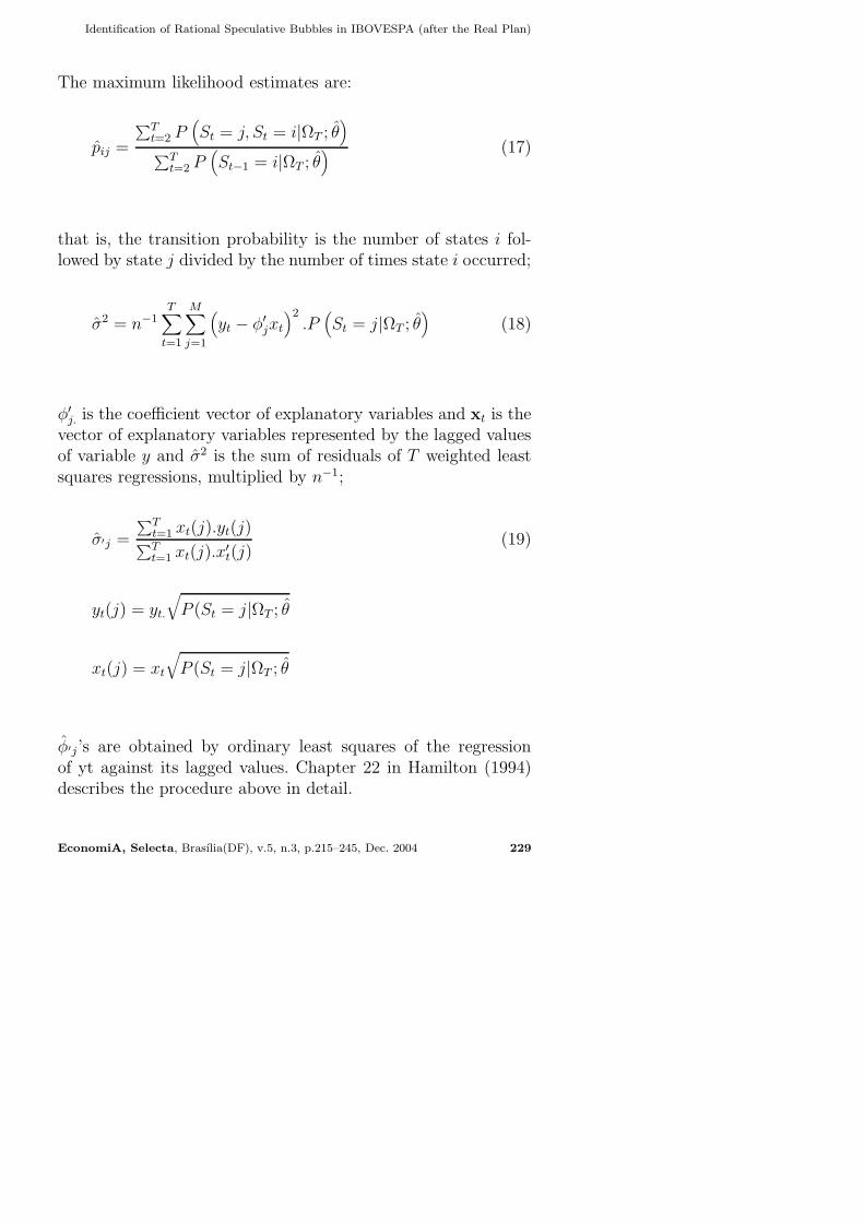
The maximum likelihood estimates are:

pij =

∑Tt=2 P

(

St = j, St = i|ΩT ; θ)

∑Tt=2 P

(

St−1 = i|ΩT ; θ) (17)

that is, the transition probability is the number of states i fol-lowed by state j divided by the number of times state i occurred;

σ2 = n−1T

∑

t=1

M∑

j=1

(

yt − φ′

jxt

)2.P

(

St = j|ΩT ; θ)

(18)

φ′

j. is the coefficient vector of explanatory variables and xt is thevector of explanatory variables represented by the lagged valuesof variable y and σ2 is the sum of residuals of T weighted leastsquares regressions, multiplied by n−1;

σ′j =

∑Tt=1 xt(j).yt(j)

∑Tt=1 xt(j).x′

t(j)(19)

yt(j) = yt.

√

P (St = j|ΩT ; θ

xt(j) = xt

√

P (St = j|ΩT ; θ

φ′j’s are obtained by ordinary least squares of the regressionof yt against its lagged values. Chapter 22 in Hamilton (1994)describes the procedure above in detail.



3 Empirical Tests

3.1 Estimation

According to Krolzig (1998), the determination of the number ofregimes, based on some test statistics, is not possible due to thenonexistence of a standard asymptotic distribution. This occurs,especially with regard to the likelihood ratio (LR), in function ofnuisance parameters that are necessary for the estimation. Thus,the initial selection of the number of regimes was made using thetheoretical framework of the speculative bubble model, whichranges from 2 to 3 regimes. The estimation results for the modelwith three regimes were omitted, due to the significance level ofmost parameters.

The procedure suggested by Granger (1992) apud Franses andVan-Dijk (2002) was used to estimate the model. This proceduregoes from the specific model to the general one, in which 1) thelevel of autoregressivity of the corresponding linear model wasobserved, 2) the null hypothesis of linearity was tested in relationto the alternative model, 3) the alternative model was estimatedand 4) the diagnostic test was eventually carried out.

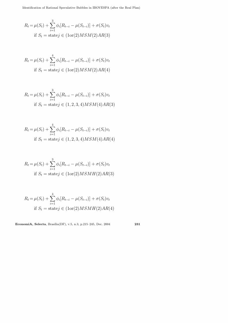
The data refer to the monthly undeflated returns of IBOVESPA,from July 1994 to March 2004. The MSVAR software (Hans-Martin Krolzig) was used in the estimation. Two situations weretaken into account: 1) the variable conditional mean, by suppos-ing the same and constant conditional variance in each regime,MSM(M)−AR(p) restrictive models and 2) variable mean andconditional variance in each regime, MSMH(M)−AR(p) non-restrictive models, as shown by the following equations:



Rt = µ(St) +3

∑

i=1

φi[Rt−i − µ(St−i)] + σ(St)vt

if St = statej ∈ (1or(2)MSM(2)AR(3)

Rt = µ(St) +4

∑

i=1


if St = statej ∈ (1or(2)MSM(2)AR(4)

Rt = µ(St) +3

∑

i=1


if St = statej ∈ (1, 2, 3, 4)MSM(4)AR(3)

Rt = µ(St) +4

∑

i=1


if St = statej ∈ (1, 2, 3, 4)MSM(4)AR(4)

Rt = µ(St) +3

∑

i=1


if St = statej ∈ (1or(2)MSMH(2)AR(3)

Rt = µ(St) +4

∑

i=1


if St = statej ∈ (1or(2)MSMH(2)AR(4)



Rt =µ(St) +3

∑

i=1


if St = statej ∈ (1, 2, 3, 4)MSMH(4)AR(3)

Rt =µ(St) +4

∑

i=1


if St = statej ∈ (1, 2, 3, 4)MSMH(4)AR(4)



Table 1Estimates for MSM(M)−Ar(p) models –Situation 1

MSM(2)Ar(3) MSM(2)Ar(4) MSM(4)Ar(3) MSM(4)Ar(4)

(8,1,2) (9,1,2) (20,3,12) (21,3,12)

Mean µ1 1 (phase 1) -0.0744∗ -0.0837∗ -0.1661∗ -0.1456∗

Mean µ2 2 (phase 2) +0.0511∗ +0.0532∗ -0.0293 -0.0373∗

Mean µ3 3 (phase 3) +0.0337∗ +0.0351∗

Mean µ4 4 (phase 4) +0.0934∗ +0.0925∗

σ 0.088712 0.085184 0.065437 0.061682

Trans Prob. 11 69.73 66.32 32.08 38.14

Trans Prob. 22 12.85 33.18 67.06 63.15

Trans Prob. 33 83.92 84.21

Trans Prob. 44 70.66 72.94

Uncond. Prob. R1 29.80 28.99 10.68 11.80

Uncond. Prob. R2 70.20 71.01 22.03 19.81

Uncond. Prob. R3 45.12 46.23

Uncond. Prob. R4 22.17 22.16

Lenght of R1 3.30 2.97 1.47 1.62

Lenght of R2 7.78 7.27 3.04 2.71

Lenght of do R3 6.22 6.33

Lenght of R4 3.41 3.70

Obs. R1 34.6 33.3 11.90 13.20

Obs. R2 79.4 79.7 25.20 22.60

Obs. R3 50.70 51.40

Obs. R4 26.20 25.80

LRmsw test 5.8736 5.7830 24.0539 24.6918

P-value (0.0154) (0.0162) (0.0000) (0.0000)

(0.1179)+ (0.1227)+ (0.0006)+ (0.0004)+

Obs: ∗ the parameters are significant at 5%.

∗∗∗ (p,r,n) where p=no. of parameters; r=no. of restrictions and n=no. of nuisance parameters.

+ the procedure of Davies apud Krolzig (1998).

Source: the authors.



In the first situation, the null hypothesis of linear relationshipbetween the variables (LRmsw test ∼ χ2, table 1.) is rejected.The t statistic LRmsw =Lmsw − Lar does not have a standarddistribution and its critical values are obtained by simulation,according to Hansen (1992) and Garcia (1998). There is poorevidence in the case of two regimes, resulting in the conditionalmean, and strong evidence in the case of four regimes, resultingin the conditional mean. In the case of two regimes, in the firstregime the mean is negative and in the second regime the meanis positive. Therefore, the first regime can be seen as a period ofdecrease and the second one as a period of growth. In the caseof four regimes, there are two phases with negative mean returnsand/or zero (phases 1 and 2) and two phases with positive meanreturn (phases 3 and 4). We may observe a regime with a stronglynegative mean and another one with a strongly positive mean,but with a smaller module.

By observing the unconditional probabilities and length, we maysee that in the case of four regimes, persistence is higher in phase3 (e.g.: MSM(4)Ar(4) model, p3 = 46.23% and average length of6.33 months). The sum of the lengths of the phases forms thecycle. The whole cycle lasted on average around 14 months. Inthe case of two regimes, the phase of price increases is morepersistent (e.g.: MSM(2)Ar(4) model, p2 = 71.01% and averagelength of 7.27 months). In this case, the whole cycle lasted about11 months.



Table 2Estimates for MSMH(M)-Ar(p) models – Situation 2

MSMH(2)Ar(3) MSMH(2)Ar(4) MSMH(4)Ar(3) MSMH(4)Ar(4)

(9,2,2) (10,2,2) (23,6,12) (24,6,12)

Mean µ1 1 (fase 1) -0.0253 -0.0379 -0.1785∗ -0.2728∗

Mean µ2 2 (fase 2) +0.0528∗ +0.0571∗ -0.0005 +0.0028∗

Mean µ3 3 (fase 3) +0.0478∗ +0.0557∗

Mean µ4 4 (fase 4) +0.1316∗ +0.1081∗

σ1 0.128480 0.127420 0.161100 0.150430

σ2 0.064989 0.064301 0.092489 0.098499

σ3 0.045528 0.043415

σ4 0.052475 0.048820

Trans Prob. 11 85.38 73.50 ∼ 0 ∼ 0

Trans Prob. 22 85.70 77.84 93.99 94.56

Trans Prob. 33 95.47 94.40

Trans Prob. 44 ∼ 0 49.00

Uncond. Prob. R1 49.44 45.54 7.74 4.72

Uncond. Prob. R2 50.56 54.46 37.23 51.86

Uncond. Prob. R3 47.34 34.14

Uncond. Prob. R4 7.69 9.29

Length R1 6.84 3.77 1.00 1.00

Length R2 6.99 4.51 16.63 18.39

Length R3 22.09 17.86

Length R4 1.00 1.96

Obs. R1 58 51.8 9.3 4.9

Obs. R2 56 61.2 57.3 68.8

Obs. R3 38.1 29.4

Obs. R4 9.2 9.9

LRmsw test 15.6338 14.1172 42.8925 35.8845

P-value (0.0004) (0.0009) (0.0000) (0.0000)

(0.0130)+ (0.0067)+ (0.0000)+ (0.0001)+

Obs: ∗ the parameters are significant at 5%.

∗∗∗ (p,r,n) where p=no. of parameters; r=no. of restrictions and n=no. of nuisance parameters.

+ the procedure of Davies apud Krolzig (1998).

Source: the authors.



In the second situation, the null hypothesis of linear relationshipbetween the variables (LRmsw test ∼ χ2, table 2.) is rejected.In all models there is evidence of the existence of two and fourregimes, generating conditional mean and variance. In the caseof two regimes, in the first regime the mean is not significantlydifferent from zero and in the second one the mean is positive.However, the variance of the regime with mean zero is twice ashigh as that of the regime with positive mean. Thus, the firstregime can be seen as a period of decrease and the second oneas a period of growth, and the risk of the first regime is muchhigher than the second one.

In the case of four regimes with different conditional variances,the sequence of phases is less evident than in the restrictedmodel. The most acute phase of the crisis (phase 1) may alternatewith the phase of largest growth (phase 4). This can produce asurprise effect to market agents. The most acute phase (phase 1)can also follow phase 2. By observing unconditional probabilitiesand length, one notes that in the case of four regimes persistenceis higher in phase 2, only in the MSMH(4)Ar(4) model, with p2

= 51.86% and average length of 18.39 months. In case of tworegimes, persistence is higher in phase 2, in the MSMH(2)Ar(4)model, with p2 = 54.46% and average length of 4.51 months. Inthis case, the total cycle lasted around 14 months and 8 months,supposing autoregressivity of order 3 and 4, respectively.

3.2 Diagnostic test

With regard to the number of regimes, the specification of mod-els with four regimes proved more appropriate than that withtwo regimes, according to the information criteria (table 3.). Thespecification of models with four regimes, without restriction tothe equality of variance proved the most appropriate accord-



ing to the likelihood ratio test (table 4.), except regarding theMSM(4)Ar(4) model.

Table 3Diagnostic TEsts of the Models

Criteria MSM(2)Ar(3) MSM(2)Ar(4) MSM(4)Ar(3) MSM(4)Ar(4)

AIC -1.4644 -1.4649 -1.4134 -1.4199

HQ -1.3865 -1.3768 -1.2186 -1.2142

SC -1.2724 -1.2477 -0.9334 -0.9130

LogLik. 91.4736 91.7683 100.5637 101.2227

MSMH(2)Ar(3) MSMH(2)Ar(4) MSMH(4)Ar(3) MSMH(4)Ar(4)

AIC -1.5325 -1.5210 -1.5260 -1.4658

HQ -1.4449 -1.4230 -1.3020 -1.2308

SC -1.3165 -1.2796 -0.9740 -0.8866

LogLik. 96.3536 95.9354 109.9830 106.8190

Source: the authors

According to Krolzig (1997), the selection of the models usingstatistical tests still requires a lot of improvement due to thenonlinearity of the model. In this regard, the tests for normalityof errors should consider the nonlinear nature of the data andthe tests for autocorrelation of residuals are only descriptive.



Table 4LR teste

Unrestricted Restricted Statistical Critical

model model test value at 5%

msmh(4)ar(3) msm(4)ar(3) 18.84 14.0671∗

msmh(4)ar(4) msm(4)ar(4) 11.19 14.0671

msmh(2)ar(3) msm(2)ar(3) 9.76 7.815∗

msmh(2)ar(4) msm(2)ar(4) 8.33 7.815∗

∗rejected Ho: the unrestricted model has a better specification

Source: the authors

According to Granger and Terasvirta (1993) apud Clements andKrolzig (1998), the good performance of nonlinear models“within the sample” could only be obtained “out of the sample” ifthe nonlinearity pattern were the same. On top of that, the start-ing point for the prediction is essential in order to obtain a goodresult. Therefore, nonlinear models do not provide goodpredictions “out of the sample”, considering a certainregime, but they are a good predictor of regime switch-ing. Diebold and Nasson apud Clements and Smith (1999) citeda series of reasons for the weak performance of linear models,among which is the wrong selection of some nonlinear models.

Based on the (“smoothed”) probabilities obtained, it is possibleto classify the observations according to the probable regimes towhich they belong, using M∗ = arg max Prob (St = M|YT ), asshown in Figure 1 below:



10 20 30 40 50 60 70 80 90 100 110 120

-0.5

0.0

MSM(4)-AR(4), 5 - 117RETINDICE Mean(RETINDICE)

10 20 30 40 50 60 70 80 90 100 110 120

0.5

1.0Probabilities of Regime 1

filteredpredicted

smoothed

10 20 30 40 50 60 70 80 90 100 110 120

0.5


filteredpredicted

smoothed

10 20 30 40 50 60 70 80 90 100 110 120

0.5


filteredpredicted

smoothed

10 20 30 40 50 60 70 80 90 100 110 120

0.5


filteredpredicted

smoothed

10 20 30 40 50 60 70 80 90 100 110 120

0.50

0.25

0.00

0.25MSM(2)-AR(4), 5 - 117

RETINDICE Mean(RETINDICE)

10 20 30 40 50 60 70 80 90 100 110 120

0.5


filteredpredicted

smoothed

10 20 30 40 50 60 70 80 90 100 110 120

0.5


filteredpredicted

smoothed

Fig. 1.



3.3 Conclusions

The models used are able to capture the nonlinear nature of thedata, resulting in a better specification than linear models. Thenonlinear models analyzed herein provide a better explanationabout the series, regarding it as a combination of distributions,where each probability distribution is generated by the probableregime to which it refers. It is possible to better understand thegeneration of a series of stylized facts, such as excess kurtosisand fat tails through the identification of regime, creating thedynamics of the return generating process.

The verification of statistical nature provides evidence of ratio-nal speculative bubbles. Considering the presence of two regimes,the smaller conditional volatility was that of the period in whichgrowth was more pronounced, whereas higher volatility occurredin the period with less growth. The periods of decrease in returnshave a shorter length. However, the model with four regimesseems to be more consistent with the rational speculative bub-ble model due to the presence of a more acute crisis and higherreturn at the end of the cycle. Thus, phase 1 of the model withtwo regimes can be decomposed into two phases, which wouldcorrespond to phases 1 and 2 of the model with four regimes.In its turn, phase 2 of the model with two regimes could be de-composed into phases 3 and 4 of the model with four regimes.This decomposition obeys condition M∗ = arg max Prob (St =M|YT). The phases with the smallest and highest returns (phases1 and 4) may be more appropriate for detachment or nonlinearrelationship between prices and fundamentals, as a result of ex-cessive pessimism or optimism of the agents, respectively. Thus,in the fourth regime, a larger number of naive investors mayparticipate in the market. Especially in the case of speculativebubble, the return should be increased to compensate for the



agents who speculate, which may occur in the fourth regime.

The exchange rate crises during this period strongly influencedthe Brazilian stock market. These crises include the following:Mexican Crisis in December 30, 1994; Asian Crisis in October24, 1997; Russian Crisis in August 4, 1998; and Brazilian Crisisin January 15, 1999. The Mexican and Asian crises gave rise toan acute phase of price decrease in the models with four regimesand with the same variance. The Russian crisis corresponded tothe end of an acute phase and the excessive currency devaluationin Brazil originated an increase in prices (phase 4) in the modelswith four regimes and with the same variance.

4 Final Remarks

The existence of rational speculative bubbles implies regimeswitching. Detecting the presence of bubbles based on regimeswitching, without considering what happened to the dividends,is the evidence that bubbles exist, according to the specula-tive bubble model. However, regime switching may occur dueto macroeconomic fundamentals, for instance, excess liquidity.In the present study, the flow of dividends was not assessed.Nevertheless, BOVESPA had to cope with a series of externaland domestic crises. Moreover, Brazil went through some re-forms, trade liberalization and changes in regulatory milestones,mainly from 1994 to 1998.

Regime switching, for example, as a result of some exogenousshock, may cause bubble collapse or predispose to it. However,this is not necessarily the harbinger of a collapse. The externalshock may be either a sign of growth or collapse.

The use of Markov switching models is relatively recent in Brazil



and promptly results in new studies. A suggestion for new stud-ies is the incorporation of the GARCH effect into the Markovswitching model, applied to the Brazilian stock market or therelationship of IBOVESPA returns with the flow of dividends inthe same model. Another suggestion is the use of more complexswitching models, such as the equilibrium correction model pro-posed by Krolzig and Toro (1999), considering the relationshipbetween returns and negotiated volume.

References

Barone, E. (1990). The Italian stock market: Efficiency and cal-endar anomalies. Journal of Banking and Finance, 14:483–510.

Blanchard, O. J. (1979). Speculative bubbles, crashes and ratio-nal expectations. Economic Letters, 3:387–389.

Blanchard, O. J. & Watson, M. W. (1982). Bubbles, rationalexpectations and financial markets. NBER Working PaperSeries 945, 1–30.

Brooks, C. & Karasaris, A. (2003). A three-regime model of spec-ulative behavior: Modelling the evolution of SP 500 compositeindex. Working paper May.

Clements, M. P. & Krolzig, H. M. (1998). A comparison of theforecast performance of Markov-switching and threshold au-toregressive models of US GNP. Econometrics Journal, I:C47–C75.

Clements, M. P. & Smith, J. (1999). A Monte Carlo study of theforecasting performance of empirical setar models. Journal ofApplied Econometrics, 14:123–142.

Coe, P. J. (2002). Financial crisis and the great depression:A regime switching approach. Journal of Money, Credit andBanking, 34(1).

Dempster, A. P., Laird, N. M., & Rubin, D. B. (1977). Maximum



likelihood from incomplete data via EM algorithm. Journal ofthe Royal Statistical Society, pages 1–38. B39.

Franses, P. H. & Van-Dijk, D. (2002). Non-Linear Time SeriesModels in Empirical Finance. Cambridge University Press.

French, K. R. (1980). Stock returns and the weekend effect.Journal of Financial Economics, 8:55–69.

Garcia, R. (1998). Asymptotic null distribution of the likelihoodratio test in Markov switching models. International EconomicReview, 39(3):763–788.

Granger, C. W. J. (1992). Forecasting stock market prices:Lessons for forecasters. International Journal of Forecasting,8:3–13.

Granger, C. W. J. & Terasvirta, T. (1993). Modelling NonlinearEconomic Relationships. Oxford University Press, Oxford.

Hamilton, J. D. (1989). A new approach to the economic analysisof nonstationary time series and the business cycle. Economet-rica, 57(2):357–384.

Hamilton, J. D. (1994). Time Series Analysis. Princeton Uni-versity Press, Princeton, N. J.

Hansen, B. E. (1992). The likelihood ratio test under non-standard condition: Testing switching model of GNP. Journalof Applied Econometrics, 7:561–582.

Jensen, M. C. (1978). Some anomalous evidence regarding mar-ket efficiency. Journal of Financial Economics, 6:95–101.

Kindleberger, C. P. (1989). Manias, Panics and Crashes: A His-tory of Financial Crises. Macmillan London.

Krolzig, H. M. (1997). Markov-switching vector autoregressions– modelling, statistical inference and applications to businesscicle analysis. Lectures Notes in Economics and Mathematics,454. Berlin, Springer Verlag.

Krolzig, H. M. (1998). Econometric modelling of Markov-switching vector autoregressions using MSVAR. Departmentof Economics, University of Oxford, Dec.

Krolzig, H. M. & Toro, J. (1999). A new approach to the anal-



ysis of business cycle transitions in a model of output andemployment. Journal of Business and Economic Statistics,21:196–211.

Laurini, M. P. & Portugal, M. S. (2002). Markov switching basednonlinear tests for market efficiency using the R/US exchangerate. In Anais Do XXIV Encontro Da Sociedade Brasileira deEconometria.

Leroy, S. & Porter, R. (1981). The present value relation: Testsbased on variance bounds. Econometrica, 49(3):555–574.

Maheu, J. M. & Mccurdy, T. H. (2000). Identifying bull and bearmarkets in stock returns. Journal of Business and EconomicStatistics, 18(1):100–112.

Mankiw, G., Romer, D., & Shapiro, M. (1985). An unbiasedreexamination of stock market volatility. Journal of Finance,40:677–687.

Mattey, J. & Meese, R. (1986). Empirical assessment of presentvalue relations. Econometric Review, 4:171–234.

Mcqueen, G. & Thorley, S. (1994). Bubbles, stock returns andduration dependence. Journal of Financial and QuantitativeAnalysis, 29:379–401.

Ryden, T., Terasvirta, T., & Asbrink, S. (1998). Stylized factsof daily return series and the hidden Markov model. Journalof Applied Econometrics, 13:217–244.

Shiller, R. (1981). Stock prices and social dynamics. BrookingPapers on Economic Activity, 2:457–510.

Summers, L. H. (1986). Does stock market rationally reflectfundamental values? The Journal of Finance, 41(3):591–602.

Terra, M. C. T. & Valadares, F. E. C. (2003). Real exchangerate misalignments. Ensaios Economicos EPGE 493.

Tobin, J. (1984). On the efficiency of the financial system. LloydsBank Review, 153:1–15.

Turner, C. M., Startz, R., & Nelson, C. R. (1989). A Markovmodel of heteroskedasticity risk and learning in the stock mar-ket. Journal of Financial Economics, 25(1):3–22.



Tversky, A. & Kahneman, D. (1981). The framing of decisionsand the psycology of choice. Science, 211.

Valls-Pereira, P. L., Hwang, S., & Satchell, S. E. (2004). Howpersistent is volatility? an answer with stochastic volatilitymodels with Markov regime switching state equations. Work-ing paper, Ibmec Business School.

Van-Norden, S. & Schaller, H. (1993). The predictability of stockmarket regime: Evidence from the Toronto stock exchange.Review of Economics and Statistics, pages 505–514. Notes.

Van-Norden, S. & Schaller, H. (1996). Speculative behavior,regime-switching and stock market crashes. Working paper96–13. Bank of Canada.

Van-Norden, S. & Schaller, H. (1997). Fads of bubbles. Workingpaper 97–2. Bank of Canada.

Weil, P. (1987). Confidence and the real value of money in over-lapping generation models. Quarterly Journal of Economics,102(1):1–22.

West, K. D. (1987). A specification test for speculative bubbles.Quarterly Journal of Economics, 102:553–580.


identiﬁcation of rational speculative bubbles in ibovespa...

Documents