rational speculative bubbles: an empirical investigation of the
TRANSCRIPT

This is the authors’ accepted manuscript of an article published in the
Bulletin of Economic Research. The definitive version is available at
www3.interscience.wiley.com

1
Rational Speculative Bubbles:
An Empirical Investigation of the London Stock Exchange
by C. Brooks, ISMA Centre, University of Reading, UK,
and A. Katsaris, ISMA Centre, University of Reading, UK
Abstract
In recent years, a sharp divergence of London Stock Exchange equity prices from
dividends has been noted. In this paper, we examine whether this divergence can be
explained by reference to the existence of a speculative bubble. Three different empirical
methodologies are used: variance bounds tests, bubble specification tests, and
cointegration tests based on both ex post and ex ante data. We find that, stock prices have
diverged significantly from their fundamental values during the past six years, and that
this divergence has all the characteristics of a bubble.
August 2001
Keywords: Stock market bubbles, fundamental values, dividends, variance bounds, cointegration, bubble specification tests.
JEL Classifications: C51, G14
Corresponding author (e-mail: [email protected]; tel: (+44) (0) 118 931 67 68;
fax: (+44) (0) 118 931 47 41) . Both authors are members of the ISMA Centre, Department of Economics,
University of Reading, Whiteknights, Reading, Berks. RG6 6BA. The authors are grateful for comments
from two anonymous referees. The usual disclaimer applies.

1. Introduction
October 24th 1929 will always be remembered as ‘Black Thursday’ since in one day 13 million
shares of trading volume forced the Dow Jones Industrial Average to show losses of 39.6%
within a week. Wanninski (1978) claims that this ‘correction’ in prices was expected as the stock
market was overvalued due to the presence of a speculative bubble. Fifty-eight years later, on
October 19th 1987, the Dow Jones Industrial Index showed colossal losses of 20%. President
Reagan commented that ‘the collapse of prices has nothing to do with economic fundamentals’1.
The evolution of prices during these two periods is very similar as both bull markets started in the
second quarter of the year (1924 and 1982 respectively) and lasted 63 months. Market prices
peaked in the third quarter of the year (3rd
September 1929 and 25th August 1987) and 54 days
elapsed between this peak and the market collapse.
The evolution of prices during these two periods raises serious questions concerning market
rationality and the relevance of fundamental values. Several researchers attribute this movement
of prices to irrational investor herd behaviour. This conclusion is however rejected by rational
bubble theory that claims that investors were acting rationally in inflating prices as they were
being compensated for it. In the recent literature, several theories that try to explain price
movements through investor behaviour models have come to the conclusion that if there was a
bubble in the stock market during these two periods, then this was created by sound and rational
investor expectations. In effect this theory attributes stock market ‘booms’ and crashes to intrinsic
bubbles.
The fundamental value of a security, according to Lucas (1978), is the present value of all the
security’s future cash flows. The divergence of the actual price of a financial asset from its
fundamental value is called a bubble. Speculative bubbles have the special characteristics that
they are persistent, systematic and increasing deviations of prices from their fundamental values
(Santoni, 1987). Speculative bubbles can be created by exogenous factors that have no correlation
with the factors that affect fundamental values, by the incorrect estimation and analysis of market

3
fundamentals, or by the presence of informational asymmetries and herd behaviour in the market
itself. According to Flood and Hodrick (1990), speculative bubbles are self-fulfilling prophecies.
Keynes (1936) noted that ‘…an equity market is an environment in which speculators anticipate
what average opinion expects average opinion to be…’. If speculators can correctly forecast this
opinion, they can earn abnormal profits by trading ahead of the market. In the case of a
speculative bubble, if they correctly anticipate the presence of such an anomaly, their buying
strategy will create excess demand in the stock market and thus cause an abnormal increase in
prices. In this way a speculative bubble will be generated.
Speculative bubbles are generated when investors include the expectation of the future price in
their information set. In a universe comprising a finite number of securities and finite investment
horizons, the expected future price will have a significant weight in the investor’s information set
and will affect his demand and supply functions. Under these conditions, the actual market price
of the security, that is set according to demand and supply, will be a function of the future price
and vice versa. As shown in the next section, in the presence of speculative bubbles, positive
expected bubble returns will lead to increased demand and will thus force prices to diverge from
their fundamental value. If the expectation of positive excess returns remains unchanged and the
investor is compensated for the increased risk of bubble collapse, then these excess or abnormal
returns will be realised in an increasing fashion.
Gilles and LeRoy (1992) have shown that every continuous dynamic price system can be
divided into two parts: a fundamental and a bubble component. The present value of the
fundamental price can be described as a linear combination of its parts, i.e. the future dividends.
However, the speculative or bubble component is larger than the linear combination of its future
elements. This in fact means that the bubble is actually bigger than the present value of its
expected future price. In the section that follows these implications are shown using the classic
dividend discount model.
1 Press Conference 20/10/1987

4
This paper will describe the theory of bubbles and collect together several techniques for the
detection of bubbles in the stock market. We will begin by summarising the theoretical
background of speculative bubbles in section 2. Section 3 will refer to three different approaches
to bubble identification including tests for bubble premium, excess volatility and cointegrating
relationships between dividends and prices. Section 4 describes the data employed, while results
from application of the techniques for bubble detection to the Financial Times All Share Index
are presented in section 5. Section 6 will conclude.
2. Theories of Bubbles
The Dividend Discount Model states that the fundamental value of the stock is equal to the
sum of all future discounted dividends:
piE dt
f
g t t gg
1
11 ( )( ) (1)
where pft is the fundamental price at time t, dt is the dividend at period t, i is the market discount
rate or alternatively the required rate of return (assumed constant – see below), and E(.) is the
mathematical expectation operator.
However, the actual price in the market deviates from this fundamental value and can be
described by the relationship:
tt
f
t
a
t ubpp (2)
where pta is the actual price of the stock at period t, bt is a bubble or deviation component, and ut
is a random disturbance term. The bubble component causes the systematic positive divergence of
prices from their fundamental values. There are several types of bubbles such as sunspots, fads,
intrinsic or speculative bubbles that have different characteristics and are generated by different
factors. Our analysis will be restricted to speculative bubbles.
In the case of speculative bubbles, investors observe that the stock is overvalued but they are
not willing to close out their position in the stock because the bubble component offers at least

5
the required rate of return. Data from 1987 show that before the October 1987 crisis, 70% of
private and 85% of institutional investors knew that the market was overvalued but they did not
liquidate their holdings.
For a rational speculative bubble to exist, the bubble component of equation (2) must grow by
at least the required rate of return (i). This means that the no arbitrage rule must hold for the
bubble component of the actual price so the bubble in period t+1 must satisfy the relation:
Et( bib tt )1()1 (3)
Under the assumption of rational expectations we can solve equation (3) for the bubble
component of period t:
bE b
it
t t
( )
( )
1
1 (4)
Equation (4) states that, since the price of period t is a function of all its future cash flows, the
bubble in period t must be the discounted future value of the bubble in period t+1. The condition
given by equation (3) must hold in order to ensure the absence of risk-free profitable trading
opportunities, and to ensure that the bubble components are discounted at the same rate that they
grow at. Assuming there is a starting value for the bubble, b0, we can solve recursively equation
(4) for the bubble at period t=0:
t
t ibb )1(0 (5)
From equations (1), (2) and (5) we can see that:
t
t
ggttg
a
t uibdEi
p
)1()(
)1(
10
1
(6)
Relationship (6) describes the effect the bubble component has on the price of the stock at
period t. The actual price at period t differs from the fundamental price given from the dividend
discount model by the second term on the right hand side of the equation. A rational speculative
bubble exists when both the fundamental and the bubble component of the price grow by at least

6
the required rate of return2. In other words, rational speculative bubbles exist when the bubble
component in the actual price grows in expected terms by at least the same rate as the discount
rate. In this case the investor cannot earn abnormal profits by shorting the asset and buying it at a
future date (Gilles and LeRoy (1992)).
However, the bubble component is a random variable and so equation (3) can be expressed as:
b i b et t t+ 1 11( ) + (7)
where et+1 is the deviation of the bubble at t+1 from its expected value and so it is the ‘surprise’
in the asset’s bubble:
e b E bt+ t t t1 1 1 ( ) (8)
This disturbance term is assumed to follow a normal distribution with an expected value of
zero and a constant finite variance (Blanchard (1979))
)σ N(0,~ 2
1t+e (9)
If equations (7), (8) and (9) hold, then the bubble component will increase at a constant rate (i)
for infinite time. This implication is not realistic since this would lead the actual price of the asset
to diverge infinitely from its fundamental value.
Blanchard (1979) modified the above equations and showed that that the bubble component
will continue to grow for a finite period with explosive expectations and will then crash leading
the actual price to its fundamental value. This explosive behaviour of bubble returns compensates
the investor for the increased risk as the bubble grows in size. In mathematical terms, Blanchard
showed that if the bubble survives, then the expected bubble at period t+1 is:
ttt biq
bE )1(1
)( 1 (10)
where q is the probability that the bubble will continue to exist in period t+1, (0<q<1)
On the other hand the bubble might burst in period t+1 with probability 1-q and in that case:
0)( 1 tt bE (11)
2 Fama and French (1988) claim that the expected or required return of an asset is the discount rate that

7
If the bubble does not burst then the investor will receive a bubble return given by the
equation:
t
ttt
bb
bbEr
)( 1 (12)
where rb is the bubble return component in the return of the stock.
According to (10), if the bubble survives, the size of the bubble at t+1 is given by:
11 )1(1
ttt e biq
b (13)
Setting the error term to its expected value of zero, if we substitute (13) into (12) we will see
that the return of the bubble component is bigger than i, which is the required rate of return, and
equal to:
)1(
q
qirb
(14)
Equation (14) expresses the explosive nature of bubble returns because as the probability of
the bubble continuing to exist gets smaller, the return of the bubble component gets
disproportionately larger. Equation (14) is in accordance with the assumption that risk averse
investors require higher return as risk increases. Van Norden and Schaller (1996) have shown that
the probability q of the bubble continuing to exist, is a function of the bubble’s relevant size
compared with the stock price. Under this setting q can be expressed as:
)( tt bfq (15)
From the characteristics of bubble returns it can be shown that:
0)(
0)(
2
2
t
t
t
t
b
bf and
b
bf (16)
The behaviour of the bubble survival probability forces equation (13) to grow at geometric
rates and so the bubble differential equation is not bounded unless the bubble bursts. This
condition rules out the existence of negative speculative bubbles because equations (2) and (14)
relates a present value with its future cash flows.

8
would imply that the stock price would become negative in finite time, since the fundamental
component does not grow as fast as the bubble component. Furthermore, from equations (7)
through (14) we see that bubble self-creation is an impossibility. If the bubble at period 0 is zero
then, as the expected value of the error term is also zero, the expected bubble for period t+k
(where k [1,)), has an expected value of zero (Evans (1991)).
This is a weakness of the above methodology for the analysis of speculative bubbles, as the
theory suggests that if a speculative bubble is expected, then investor behaviour will create it3.
Modern theories of investor behaviour and game theoretic approaches that model information
inefficiencies or temporary investor irrationality provide useful analytical tools that explain and
model bubble self-creation4.
Equation (6) is a first order expectational difference equation. For this equation to have the
forward-looking solution given by equation (1), then it must be driven by a convergent sum.
However, equation (6) implicitly makes unrealistic assumptions about the universe in which
decisions are taken. These assumptions are: a constant discount rate, constant dividends, a finite
and constant number of investors, who have infinite planning horizons5, perfect foresight and face
an unlimited information set. To make this model more realistic, we restrict the investor’s
planning horizon to period T (where T<), we adjust for conditional expectations of future
values, under a restricted information set (Φt) and we include an expected variable discount rate.
Furthermore, we cut off the forward looking solution at a terminal price and substitute the infinite
sum of future dividends with the price at t+T, pt+Ta. Equation (6) can thus be rewritten as:
))(())((1=g
t
1 1s
t
a
Tt
T
gtt
T
g
gt
g
gtt
a
t pEdjEp
(17)
3 Brock (1982), Tirole (1982), Gray (1984) all point out that temporary investor irrationality or
asymmetries in the market information dissemination mechanism might be cause for the generation of
speculative bubbles. Furthermore intrinsic bubbles that are based on fundamentals are generated constantly
through investor’s expectations. 4 For example, Lux (1995), Kirman (1993)
5 or maximise utility with an overlapping-generations model.
9
where jt is the variable dividend discount factor, )1()1( ttt ilj , t is the expected variable
price discount factor, lt is the expected variable dividend growth, it is the excepted variable
discount rate, and t is the information set investors use to form their expectations of future
dividends and the future price at period t.
If a speculative bubble exists, the bubble component in equation (15) is included in the future
price pt+T. For a bubble not to exist, the transversality condition implied by equation (18) below
must hold and the difference equation must have a terminal condition. In other words, the
difference equation must be bounded and must converge. These conditions are fulfilled if and
only if:
0))((1
lim
t
a
Tt
T
g
gttT
pE (18)
and
T
g
T
ggttgtt iElE
1 1
))1(())1(( (19)
Given the properties of the bubble component described in equations (13) to (16), if a
speculative bubble is present then equation (18) will not hold since the bubble is an unbounded
explosive difference equation without a terminal condition. This is shown from equation (14)
since the bubble grows faster than the discount rate. In other words, if (18) and (19) hold then
equation (17) is bounded and has only one solution, which is a price that depends only on
fundamental cash flows (Khon (1978)). This is the fundamental price and is denoted ptf:
p E j dt
f
t t g t g
g
( ( ) )g=1
tΦ1
(20)
Many researchers use equations (17) through (20) to test for the presence of speculative
bubbles; these equations will be used in this study also. We can see that the future dividends are
in an expected form so in order to test the existence of bubbles, expected dividends must also be
modelled. Some researchers take the ex-post known values for dividends assuming investor
perfect foresight. However, we instead model dividends or dividend growth and find fundamental
10
values using an information set that is similar to the investor’s. The next section will briefly
describe several ways of testing for speculative bubbles.
3. Tests for Bubbles
There are several approaches to test for the presence or otherwise of speculative bubbles.
These approaches can be grouped into three main categories: tests for bubble premiums, tests for
excess volatility and tests for the cointegration of dividends and prices. All of these methods will
be described below.
3.1 Tests for a Bubble Premium
The fundamental return of a stock can be divided into the risk free return, the risk premium
that compensates the investor for the risk of the stock, and a random disturbance. A bubble
premium is the excess return the investor demands above the fundamental return in the presence
of a speculative bubble. This return has an explosive nature as it increases geometrically through
time. This return is incorporated in the actual excess return of the stock over the risk free rate.
Hardouvelis (1988) examines the presence of a bubble premium in the New York, London and
Tokyo stock market indexes for the period 1977-1987. This model included proxy variables for
the time risk, corporate risk and market risk of the investor as well as some variables of dividend
and debt policy of the aggregate stock market. His results show that the model was able to
forecast actual excess returns for the period 1977-1985 but parameter stability tests showed a
breakpoint in the data after March 1985. Hardouvelis suggests that this breakpoint implies that
returns before this date where ‘bubble free’. He thus calculates the bubble premium by simply
subtracting the excess return of the 1977-1985 period from the 1985-1987 excess return and finds
the presence of a positive and increasing bubble premium for 18 months before the Crash of
October 1987.
However, his analysis is based on several arguably dubious assumptions. To calculate the
bubble free excess return, he assumes that there is no bubble in the first sample period, a
11
hypothesis that is unsubstantiated. Furthermore, he assumes that the slope coefficients of the
model predicting excess returns for the first period remain constant in the second period so that he
can simply subtract the excess return of period one from the return of period two and calculate the
bubble premium.
Another, indirect, method for testing the existence of a bubble premium in stock market
returns was developed by Rappoport and White (1993). Their approach used the interest rates of
brokers’ loans to detect the presence of bubble in the years before the 1929 stock market crash.
They observe that the interest rate of these loans and their premium, over the inter-bank interest
rate, increased substantially in 1928 and 1929. This increase implies that the creditors of that
period had perceived an increase in the market risk that was caused by the presence of a
speculative bubble. DeLong, Bradford and Shleifer (1987), come to the same conclusion by
observing the premium of closed end funds for the same period. Their analysis concludes that
differences in investors’ and fund managers’ expectations of future earnings might have caused
an abnormal increase of this premium, as investors have been accused of over-optimistic
expectations in the period leading up to the October Crash (Galbraith (1988)).
However, the above indirect methodology is criticised by Liu, Santoni and Stone (1995), (LSS
hereafter), since they observe a similar pattern of interest rates and premiums in 1919-1920. If
Rappoport and White are correct, there must have been a bubble in the stock market in that period
as well but it did not crash. In their critique, LSS suggest that the increase in interest rates was
caused by the tight monetary policy followed by the FED in these periods, and they test the time
series of interest rates for the presence of a breakpoint. The results show that the process of
interest rates and premiums remained unchanged for the whole period, and so they reject the
hypothesis of the presence of a bubble.
3.2. Excess Volatility Tests
The broad consensus of the literature is that tests for the presence of a bubble premium faced
serious problems and were not able to prove or adequately disprove the existence of speculative

12
bubbles. A different method of testing for bubble existence is by examination of the stock
market’s variance and the application of tests for excess volatility. In general, if a speculative
bubble is present, the variance of the stock price will be greater than the variance of the
fundamental price. Although Friedman (1953) claims that the presence of speculators decreases
the volatility of prices, Hart and Kreps (1986), Baumol (1957) and Kohn (1978) show that
speculators and speculative bubbles cause a significant increase in price volatility.
Tests for the presence of excess volatility are based on a comparison of the variance of actual
prices with the variance of fundamental prices. In most cases, the fundamental prices are
constructed using ex-post analysis, but several researchers try to model and forecast dividend
series in order to construct fundamental prices that are similar to the prices perceived by
investors.
Shiller (1981) performs the first tests for excess volatility by comparing the volatility of actual
prices and fundamental prices that were constructed using ex-post analysis. These rational,
fundamental prices are constructed using real dividend data, assuming investor perfect foresight,
and a constant discount rate. The fundamental price series includes a terminal condition for the
sum of discounted dividends and the infinite sum was substituted with the price of the S&P in
1979. The variance of these prices is then compared with the variance of actual stock prices.
Variance Bounds Tests are built on the assumption that the variance of actual prices should be
smaller than the variance of fundamental prices since:
)()()()( a
tt
a
t
f
t pVaruVarpVarpVar (21)
Shiller uses price and dividend data for the S & P 500 Index for the period 1971-1979 and de-
trends the two time series for inflation and earnings volatility. The results of the variance bounds
tests show that condition (21) was almost always violated by the data, indicating that a bubble
was present in the market. However, this method for constructing fundamentals is limited since
the cut-off point was chosen arbitrarily. Moreover, the substitution of the infinite sum of
discounted dividends with the actual price of 1979 makes the implicit assumptions that the market

13
efficiently priced future cash flows in that year and that the dividend process remained unchanged
for out of sample dividends. Marsh and Merton (1986) show that the construction of fundamental
prices using an inappropriate assumption for the dividend process can lead to the wrong
conclusion regarding bubble presence, especially if dividends are generated from a non-stationary
process (Dybvig and Ingersoll (1996)). Furthermore, the construction of fundamental prices using
a constant discount rate is based on the unrealistic assumption that investor risk aversion and
market risk remain constant through time. In this context, the excess volatility tests will almost
always reject the no-bubble hypothesis.
Shiller (1997) adjusts equation (21) for dividend non-stationarity, but his improved variance
bounds tests still use a cut-off price as an estimate of the infinite sum of discounted dividends and
a constant discount rate. In an effort to deal with changing investor risk aversion, Grossman and
Shiller (1971) insert a variable discount rate that is generated from a variable risk aversion utility
function. Their results show that although these ex-post fundamental prices have increased
variance, the no-bubble hypothesis is again rejected, as actual prices are still more volatile.
However, all volatility tests, that use fundamental prices which are constructed using cut off
prices as proxies for the discounted sum of future dividends, are unreliable since the terminal
price might contain a bubble that will not be detected as it will be included in the fundamental
price. In a more general critique, Kleidon (1986) shows that excess volatility might not be caused
by the presence of a bubble, but rather by investor irrationality or fundamental model
misspecification. In essence, Kleidon states that fundamental prices constructed with ex-post data
are different to prices observed by investors, since investors’ forecasts are made under
uncertainty. Perfect forecast prices are constructed with 100% certainty so they represent only
one of the infinite economies faced ex-ante by investors.
LeRoy and Porter (1981) build fundamental values that use dividends that are forecasted based
only on historical information, but after testing their model on S&P 500 data, they come to the
same result that equation (21) does not hold. Dezhbakhsh and Demirguc-Kunt (1990) use an

14
ARMA model to forecast dividend series and construct fundamental values using these expected
dividends. Using the same data for the S&P 500 they cannot reject the no-bubble hypothesis and
find that fundamental and actual values have the same volatility. West (1987) uses the same
ARMA modelling methodology, but decomposes the variance bounds test into three separate tests
of model specification, data consistency and excess volatility. His methodology comes to the
conclusion that a bubble is existent in the data.
Overall, Flood and Garber (1980) claim that variance bounds tests are in general unreliable.
They argue that most of the models for fundamental price construction are misspecified, and are
not formed with an information set similar to the one that investors use, and more importantly,
they exclude relevant variables. Furthermore, they use dividend and price series that are
nonstationary, which could lead to biased variance estimates.
3.3. Non-Stationarity and Cointegration Tests
Diba and Grossman (1988a and 1988b) show that if the stock price depends exclusively on
future dividends, if there are no rational speculative bubbles and if dividends are stationary in the
mean, then prices will be stationary. However, even if dividends and prices are non-stationary, if
they are cointegrated then the no-bubble hypothesis cannot be rejected. Nevertheless, the lack of
cointegration is not a sufficient condition to prove the existence of bubbles since the model might
exclude significant variables that affect stock prices and that are not stationary. In their survey,
Diba and Grossman find that the dividend and price series for the S&P 500 are difference
stationary so they reject the bubble hypothesis, and after testing for cointegration, they verify
their result of no bubble since prices and dividends are cointegrated. However, Dickey Fuller tests
for unit roots give unreliable results for samples of the sizes used in the Diba and Grossman study
(less than 100 observations) – see Evans and Savin (1984).
Campbell and Shiller (1987) come to the same conclusion by testing the difference of prices
and discounted dividends for stationarity. They use only historical information to forecast
dividends and returns and test their model on U.S. stock price and dividend data. Their results

15
show that the linear combination of prices and discounted dividends is an integrated series of
order one so there is evidence of a bubble but they note that this methodology is very sensitive to
the discount rate used. Craine (1993) has shown that the discount rate for the S&P 500 is
nonstationary, and so the nonstationarity of actual prices, even if dividends are stationary, maybe
caused by the discount rate used. Fama and French (1988) support the above conclusion and show
that prices follow a stationary evolution process for short term horizons, but this process varies as
the time horizon is increased. According to their analysis, stock prices can be predicted in part,
but the classic present value model does not hold because of the presence of collapsing and
regenerating bubbles that cannot be detected. The presence of such bubbles is supported by
Summers (1986) who claims that expectations or bubbles that are based on expectations might
cause a significant temporary divergence of actual prices from their fundamental values, but such
bubbles do not leave a statistical trace and so cannot be identified.
Johansen (1991) shows that a lack of cointegration of dividends and prices might not be
caused by the presence of a bubble but by the lack of cointegration in reality caused by other
factors. In addition, Evans (1991) states that cointegration tests cannot detect a large category of
bubbles that are based on fundamentals. These intrinsic bubbles follow the same evolutionary
process as the expected dividend and so they cannot be detected. As a result of all of these
problems, stationarity and cointegration tests have very low power (Mattey and Meese (1986)).
A more realistic approach to modelling fundamental values is conducted by Donaldson and
Kamstra (1996). Their analysis uses an ex-ante data in an ARMA-GARCH, Artificial Neural
Network model to forecast expected discounted dividend growth and build fundamental values
with non-stationary, non-linear discount rates and dividends. The fundamental values they
construct for the 1929 U.S. stock market follow the same pattern as the actual values and mimic
the behaviour of the alleged bubble. Furthermore the discounted dividends and the actual prices
are cointegrated so the bubble hypothesis is strongly rejected. Their result is in line with Sirkin’s
(1975) view that the boom and crash was a result of rational investor expectations.
16
Finally, Campbell and Shiller (1988) have tried to model future stock prices using valuation
ratios for U.S. stock market data. Their survey finds that although returns and dividend yields
demonstrate very high volatility, they seem to be highly correlated with their fundamental values.
This fact shows that there is a weak cointegrating relationship between dividends and prices and
so the evidence of bubble existence is not reliable.
In conclusion, although tests of stationarity and cointegration cannot give reliable results for
bubble existence, since they are very sensitive to small samples and model misspecification, they
are the best analytical tool available to identify the presence of a long term relationship between
actual prices and fundamental variables. The presence of a long-term relationship between
dividends and prices can be an indication of bubble absence, but the tests greatly depend on the
method employed to construct fundamental values. An appropriately specified model for
constructing fundamental values must be based on a well-specified model of dividend prediction.
4. Data
The data that we use to perform the tests for bubble existence are the Financial Times All
Share Index monthly closing prices and a constructed FTAS dividend index from January 1965 to
March 1999. The dividend index is annualised and is derived from the monthly close dividend
yield for the same period.
To obtain an actual ‘cash’ dividend time series we take the natural logarithm of the monthly
dividend yield and then add the natural logarithm of the FTAS Index monthly close price. In this
way, we obtain the logarithm of the implied actual annual dividend. This estimate is equivalent to
a monthly cash dividend of the FTAS index. To verify that the above transformation has not
miscalculated the monthly dividends we calculate annual dividends from the monthly series,
construct dividend yields with year close prices and compare this series to the annual dividend
yield of Datastream6.
6 The average difference of the two yields is not significant and equal to -0.074% out of an average
dividend yield of 4.6901% for the period studied.
17
For graphical representation purposes, a dividend index is constructed using monthly
dividends. This index is built setting the value for January 1965 to 100, which is also the value of
the FTAS Index. Both the monthly dividend and price series are transformed into real variables
using the monthly United Kingdom Producer Price Index7. All the calculations and regressions
are performed with real data, nevertheless the results are then transformed into nominal terms
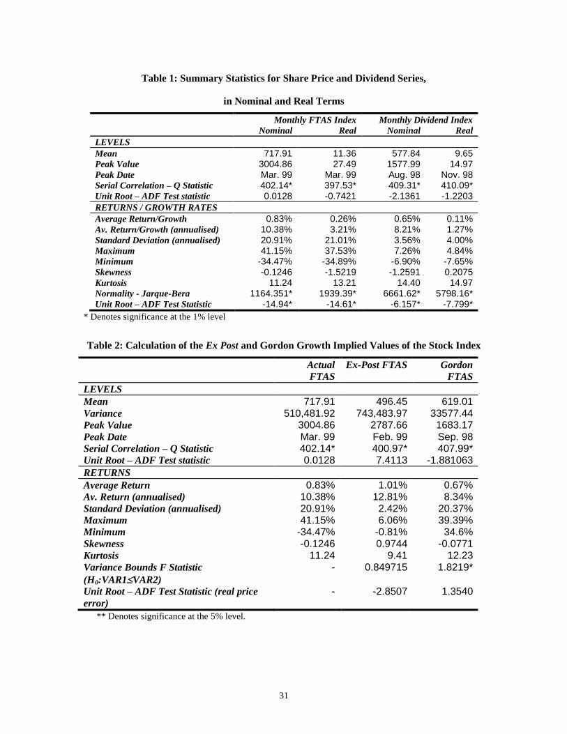
again for graphical representation to retain the visual image of the FTAS index. Some summary
statistics for both nominal and real variables are shown in Table 1.
From Table 1, we can see that both the nominal and real series are integrated series of order
one, I(1), according to the ADF test. It is clear also that the two indices differ in their peak value
and peak dates. The dividend index has had a downward trend since August 1998 revealing a
greater divergence of the FTAS index from its dividend index. From Graphs 1 and 2 it is obvious
that the price index displays more volatility and often diverges significantly from the dividend
index. This divergence was sharp in the period preceding the 1987 stock market crash and is even
greater in the last six years. In a following section we will show that the divergence of the FTAS
index from the dividend index begins in January 1993 and displays bubble behaviour.
5. Results
In the section 3, several techniques to test for bubble presence were described. Most of these
techniques used historical data to build fundamental values using classical dividend discount
methodology. In this section, two of these traditional methods for bubble identification will be
analysed. The first approach is based on comparing the variance of actual market prices to that of
fundamental values. These fundamental values are constructed using historical dividend and price
information only. According to Shiller’s (1981) methodology we construct fundamental values
using the following relationship:
1999/31 )1(
1
)1(
1P
id
ip
gT
T
ggtg
f
t
(22)
7 Obtained from Datastream

18
where ptf is the fundamental value, dt is the dividend of period t, and P3/1999 is the truncation
approximation of all out of sample dividends.
In effect, this equation constructs fundamental values assuming investor perfect foresight. The
infinite sum of discounted dividends is cut off at March 1993 and this sum is replaced with the
value of the real FTAS for that month. The discount rate used is the real monthly average return
of the FTAS for the period, which is 3.21% in annual terms. These prices are presented in Figure
3 and show a very smooth behaviour. Shiller’s methodology consisted of using variance bounds
to test for the presence of excess volatility in actual prices. The variance of these constructed
fundamental prices is 743,483.97. This variance is then compared with the variance of the actual
prices using an F-test. The result of this test is presented in Table 2. The first column of this table
contains summary statistics for the actual FTAS while column 3 reports results from the ex-post
warranted prices. The other columns report results from alternative models discussed below.
Although the F-test statistic is insignificant, implying that the variance of the actual FTAS is
not significantly greater than the variance of the fundamental values, this result should be viewed
with caution. It is clear from the graph that the fundamental values display little volatility around
their non-linear trend, while the FTAS shows substantial volatility. Furthermore as we move
towards 1999, the fundamental values are increasingly affected by the actual value of the FTAS
that is used for the truncation. For the above reasons we looked at the returns of both series and
found that although the annual average return implied by the fundamental values is greater, in
nominal terms, than the FTAS’s, this return displays significantly less volatility than that of the
actual series.
Furthermore, after testing the differences of actual and constructed values for stationarity, we
find that this error is a non-stationary series. Campbell and Shiller (1987) state that if market
prices are ‘bubble-free’, then this price error should be stationary. Identification of a rational
bubble by the difference between the stock price and the discounted future path of dividend
19
payments can be justified only under the assumption that the involved risk premium in the stock
index is stationary. In this case the conclusion is ambiguous.
As noted above, the ex-post warranted prices are formed in a 100% certain environment so
that they do not take into account the uncertainty investors are facing about future fundamental
values. Furthermore, they are based on serially correlated dividends (see table 1) so they follow a
smooth evolutionary process. In addition to the above, the replacement of the infinite dividend
series with the price of the FTAS for March 1999 is performed under the implicit assumption that
the dividend generating process will be the same for out of sample dividends.
Finally, the major problem of this approach is that it includes the actual price of the FTAS in
the fundamental construction process. If this price contains a bubble then this bubble will be
included in the fundamental value and so it will not be observed. It is clear from graph 3 that as
we approach the end of the sample period the fundamental values converge towards the actual
values as the weight of the FTAS actual truncation price increases in the fundamental price. A
more general critique to this approach is that the inputs to the fundamental value relationship are
assumed to be constant, in what concerns the interest rate, or stationary, with respect to dividends.
These assumptions are far from realistic and probably lead to misspecification of the model.
To address some of the problems mentioned above we construct more realistic fundamental
prices using the Gordon Dividend Growth Model. Using again a constant discount rate and a
constant dividend growth rate, we estimate fundamental values for the period 1993-1999 using
only data available at the start of this period. We assume that the discount rate and the dividend
growth rate are constant for the entire sample and estimate fundamental values using the
following model:
1-t )(
)1(d
ig
gp f
t
(23)
The fundamental values estimated from the above model are based only on information
available in December 1992 and are ‘updated’ every month as new information on dividends is
made known. The discount rate used is the average FTAS real return for the period January 1965
20
– December 1992 and the dividend growth rate is the average growth of real dividends for the
same period. These values are identical to the ones contained in the investors’ information set in
January 1993. The results for this methodology are also presented in Table 2 and the constructed
fundamental values are shown in Graph 4.
It is clear that after January 1993, the actual FTSE diverges from the expected fundamental
value, demonstrating increased volatility. The projected fundamental values imply a March 1993
value of the FTAS of 1600.10 points, significantly lower than the actual value of the FTAS. The
fundamental values have remarkably lower variance than the actual FTAS (33577.44 versus
196735.21 of the FTAS for the sample period). This result shows that actual prices have more
volatility than the fundamentals that should drive their evolutionary process. In Shiller’s context,
this would be evidence for bubble presence. Furthermore the actual price error is nonstationary
and so this test rejects the no-bubble hypothesis as well.
However, this approach suffers from similar weaknesses as the Dividend Discount Model
approach since the dividend growth rate and the discount rate are not constant over time.
Donaldson and Kamstra (1996) state that dividend growth has time varying conditional moments.
Furthermore the discount rate is a function of investor risk aversion. As discussed above, if
bubbles exist then the expected return grows geometrically for the bubble to survive. Even
without bubbles, investors perceive different levels of risk through time and so they modify their
discount rate accordingly. The use of a constant discount rate constructs fundamental values that
tend to reject the no bubble hypothesis.
From the results it is clear that the traditional approaches for bubble identification suffer from
specification problems, as they cannot capture the dynamic characteristics of fundamental values
in the market. The assumptions of constant discount rates or dividend growth are non-realistic
while the use of raw price and dividend data, when they are nonstationary, leads to unreliable
conclusions regarding excess volatility and bubble presence. Moreover the models used are
extremely sensitive to the stationarity of the discount rate and the dividend growth rate.
21
5.1. The Ex Ante Approach
In order to address some of the problems of traditional bubble identification procedures,
Dezhbakhsh and Demirguc-Kunt (1990) built fundamental values using a model that includes
only current and past dividends in order to approximate the investors’ information set. Their
approach tests the no-bubble hypothesis separately from fundamental model misspecification.
Fundamental values are given by the present value of all future cash flows. Under this setting,
the actual price of a security must satisfy the no-arbitrage condition given by:
)Φ)(( t11 t
a
t
a
t dpEp (24)
where is the real discount factor. This is a first order condition derived for a representative
agent’s optimization problem. The forward-looking solution to (24) is:
)Φ( t1
ggt
gf
t dEp (25)
Equation (24) does not have a single solution, as the one given by (25), and, as seen previously
the general solution is given by:
tt
f
t
a
t ubpp (26)
In order to test for bubble presence we first assume that the investor’s information set includes
information only on present and past dividends. This assumption, however unrealistic, is crucial,
as it is necessary to exclude actual prices from the fundamental estimating equation as they might
contain bubbles that will be included in the fundamental value (Grossman and Shiller, 1971). This
is equivalent to assuming that the investor’s utility function shows absolute preference to
dividend payments over capital gains8. Under this assumption equation (25) can be rewritten as:
tg
gt
gf
t zdEp
)H( t
1
(27)
8 Diba and Grossman (1988) employ the same assumption.

22
where ])H([ t1
gtg
gt
g
t ddEz
, and Ht is a subset of t that includes information only on
dividends. From equation (27) we see that the expectation for future dividends is formed based
only on information for historical dividends. This fact intuitively leads us to conclude that
dividends, in this setting, must follow a process described by:
qtqtot ddd ...11 + vt (28)
where vt is an error term. This process will be tested on our data to see if it accurately describes
dividend evolution. If this is an accurate proxy for the generating process of dividends, then
equation (27) can be rewritten as:
tqtqtto
f
t zdddp ...121 (29)
where z is serially correlated as seen from equation (27).
If we substitute equation (29) into equation (26) we will see that the actual market price will
be a function of all current and past dividends, a bubble component, if a bubble exists, and
serially correlated residuals. In this setting we have excluded intrinsic bubbles since we assume
that the bubble component is orthogonal to the dividend generating process. We thus conclude
that actual prices are given by:
ttqtqtto
a
t zbdddp ...121 (30)
Equation (30) is used to test for bubble presence. We do not formulate a specification for the
bubble term since the methodology does not require one to test for a bubble’s existence.
To accurately detect the presence of speculative bubbles, we need to ‘disengage’ model
misspecification tests from bubble presence tests. We first examine whether the specification of
the above models is correct and especially the specification of equation (24). This analysis will
allow us to determine whether the discount model explains actual market values. If this equation
is well specified then equation (29) will hold if dividends are generated by an autoregressive
process. If all the fundamental generating equations hold, then we can proceed to detect the
presence of bubbles. The no-bubble hypothesis is tested by examining the specification of
23
equation (30) after we exclude the bubble term. If this term should be included in the equation,
the model will produce biased and inconsistent coefficient estimates and the model will be
misspecified.
The results of the previous section have drawn our attention to a possible breakpoint in the
actual price series. It is therefore of interest to perform the above methodology on the whole
sample, but also to examine whether the behaviour of the above models changes in the period
1993-1999. In order to test if there is a bubble in the FTAS Index in the late 1990’s, we present
results of the above methodology on the whole sample, the period 1965-1993 and the period
1993-1999.
Our first step is to identify and estimate the dividend process. We have seen that this process
is I(1), so we perform our analysis using the first difference of the series. We identify the
dividend process as an ARIMA(1,1,1) process using Schwarz’s Bayesian information criterion, so
we have:
tttot uudd 1211 )()( (31)
The model is estimated using Maximum-Likelihood and summary results are presented in
Table 39.
To verify that this specification is adequate, we check the residuals for serial correlation and
see that the Q statistic is insignificant for 24 lags at the 5% level. Furthermore, as we suspect
(from the information contained in Figures 1 to 3) the presence of a breakpoint in January 1993,
we test the stability of the process to see if the dividend series contains a breakpoint. The Chow
test does not reject the hypothesis that the series does not contain a breakpoint at that time; we
therefore use this dividend specification for the whole sample. Finally, we perform a Ramsey
RESET test to determine whether the linear representation is sufficient; the null of no non-linear
structure is not rejected, and we therefore conclude that the ARIMA(1,1,1) model is a sufficient
model to estimate future dividends.
9 Detailed results are not presented, but are available in an appendix on demand from the authors.
24
Our next step is to examine the specification of the arbitrage model expressed in equation
(24). We perform this estimation on the whole sample and on the two sub-samples to see if the
estimate is significantly different, implying a different discount factor in the two periods. The
estimation results are presented in Table 4. The implied real discount rate from the slope
coefficient10
is a monthly 2.21%, significantly higher than the average real return of the FTAS for
the sample period. This finding shows that the traditional methods were miscalculating
fundamental values. The model does not appear to suffer from misspecification as the RESET F-
statistic is insignificant.
However, the Chow forecast test suggests that there is a breakpoint in the estimation. We can
observe a breakpoint in the series in January 1993. We thus estimate the model for the two sub
samples. We can see that the implied discount rate for the first period is much closer to the actual
average, while the value of θ for the second period is significantly higher, implying a discount
rate of 4.26%. The residuals do not show signs of autocorrelation in any of the regressions,
suggesting that investors have rational expectations.
Given the above results, we conclude that the specification of equation (24) is appropriate and
so it is possible to estimate equation (30) that is derived from it. However, since the dividend
process is an ARIMA(1,1,1), equation (30) must be expressed in differenced form. Hansen and
Sargent (1981) state that only the AR(i) term should be included in the regression so that the
actual price difference is estimated from the one lag dividend difference. Under this setting the
regression takes the form of:
tto
a
t udp )()( 11 (32)
Again, this estimation is performed for the whole sample and the two sub-samples separately; the
results are presented in Table 5.
It is clear from the estimation results that the model performs well only for the first sample,
i.e. the period 1965-1993. In effect, all of the specification tests show that actual market values
10
Calculated as (1/slope coefficient) –1.
25
were a function of the fundamental values in this period and that the bubble term has been
correctly removed from the equation. The estimation for the whole sample however demonstrates
some misspecification problems, all attributable to the characteristics of the data after 1993. We
can see that in both these cases, the fundamental term is insignificant and the RESET statistics
show that the bubble term should be included in the regression. Therefore the model suffers from
misspecification for these two periods. The results from recursive coefficient estimation seem to
support the conclusion that there was a breakpoint in the data around the aforementioned period11
.
In conclusion, the results of the above methodology seem to reject the no-bubble hypothesis
strongly. It is however possible that the bubble term does not have a speculative bubble
specification or that another unobservable factor is causing the misspecification of the
fundamental model. In order to verify our results we perform a cointegration analysis for the price
and dividend series.
5.2. Cointegration Tests
As noted above, if dividends and prices demonstrate a long-term relationship then there is no
bubble in stock market prices. We use the Johansen test to identify the presence or otherwise of
cointegrating vectors in the levels of prices and dividends. The methodology we use is similar to
that of Diba and Grossman (1988a and 1988b). If prices and dividends are integrated of order
one, which they both are (as seen from table 1), then for bubbles not to exist their linear
combination must be stationary in levels. The results of the Johansen tests are given in Table 6.
These tests clearly show that prices and dividends are not cointegrated in their levels if we
examine the whole sample. Such a result would imply that there is no long run relationship
between dividends and prices and theory would thus conclude that speculative bubbles are
present. We again examine both samples separately and the results show that a cointegrating
relationship between dividends and prices existed until 1993. This relationship disappears after
this date and so we conclude that a speculative bubble was present only after January 1993.
11
These results are not presented for brevity, but are available from the authors on request.
26
However this technique cannot detect bubbles that are based on fundamentals. This weakness
could mean that there is a bubble even in the period preceding 1993 but this bubble would not be
detected. On the other hand, the lack of cointegration may be caused by a structural change in the
long-term relationship between dividends and prices. We leave the question of tests for bubbles
based on cointegrating regressions allowing for structural breaks to future research.
6. Conclusions
In this paper we present empirical evidence from three different bubble identification
techniques for the FTAS Index. The attention of this paper was focused on the recent period of
extraordinary market growth. It should be noted that the FTAS has offered investors a return of
more than 200% over the six years 1993-1999. This price evolution has, as this paper has shown,
led market prices to diverge significantly from their observable fundamental values. Although
several methods exist for the detection of speculative bubbles, all of them are based on one
implication: are actual market prices driven by economic fundamentals?
The empirical evidence presented does not suggest so. The no-bubble hypothesis was at first
rejected by two traditional bubble identification techniques that were based on using simplified
fundamental construction models. The results of these two methods are easily questioned since
they use unrealistic assumptions and suffer from theoretical and practical misspecification
problems. This fact proved to be a useful foundation for the second technique used, which was
based on separately identifying model misspecification from bubble presence. The results of this
method reinforce our belief that the FTAS Index was not driven by market fundamentals after
1993. In fact, this methodology showed that the fundamental model that explained prices for 28
years is unable to capture recent market dynamics.
Our conclusion on the possible existence of an explosive bubble in the London Stock
Exchange was given further weight by the use of cointegration techniques, which showed that the
long run relationship between prices and dividends did not hold in the late 1990’s. This result
27
implies that other variables drove stock prices at that time. One of these variables might be a
speculative bubble.
Although the evidence we have presented is strongly in favour of bubble existence, the no-
bubble hypothesis cannot be rejected easily. It is possible that non-observable fundamental
variables, such as investor rational expectations and market sentiment, are the cause of the rapid
and sharp divergence of prices from fundamental values. The possibility of the UK joining the
full European Monetary Union or market expectations for yet another period of economic
expansion might be factors that are discounted by the market and constantly force prices to higher
levels. The models and tests currently available and employed in this paper could not take such
variables under consideration, as they are not measurable. Intrinsic bubble theory might be able to
identify and explain such phenomena.
Furthermore, it is possible that the fundamental relationship that links prices to future
dividends has changed due to shifts in investor preferences. Such factors can only be taken into
account by using game theoretic approaches (e.g. Lux, 1995) to explain investor behaviour and
expectations. Finally, divergence from economic fundamentals might be caused by investor
irrationality. If this is true, then our models, that are based on the arbitrage condition described
above, are unsuitable tools for use in an effort to explain market expectations and dynamics.
REFERENCES
Blanchard O. J.: ‘Speculative Bubbles, Crashes and Rational Expectations’, Economics
Letters, 3 (1979) 387-389
Brock W.: ‘Asset prices in a Production Economy’, International Economic review (1974) 15,
750-777
Baumol W. J.: ‘Speculation, Profitability and Stability’, Review of Econometrics and
Statistics, 39 (1957) 263-271
Campbell J., Shiller R.: ‘Cointegration and Tests of Present Value Models’, Journal of
Political Economy (1987) 95, 1062-1088
________: ‘Stock Prices, Earnings and Expected Dividends’, Journal of Finance (1988) 43,
661-676

28
Craine R.: ‘Rational Bubbles: A Test’, Journal of Economic Dynamics and Control, 17 (1993)
829-846
Dezhbakhsh Η., Demirguc-Kunt A.: ‘On the presence of Speculative Bubbles in Stock Prices’,
Journal of Financial and Quantitative Analysis, 25 (1990) 101-112
DeLong, J.B., Bradford, S., A.: ‘Noise Trader Risk in Financial Markets’, Journal of Political
Economy, 95 (1987) 1062-1088
Diba B. T. & Grossman H. I: ‘The Theory of Rational Bubbles in Stock Prices’, The
Economic Journal, 98 (1988a) 746-54
________: ‘Explosive Rational Bubbles in Stock Prices?’, American Economic Review, 78
(1988b) 520-530
Donaldson G. R., Kamstra M.: ‘ A New Dividend Forecasting Procedure That Rejects Bubbles
in Asset Prices: The Case of 1929’s Stock Crash’, The Review of Financial Studies, 9 (1996)
333-383
Dybvig P., Ingersoll J. Jr.: ‘Stock Prices Are Not Too Variable: A Theoretical and Empirical
Analysis’, Notes for the Finance Seminar, University of Chicago (1996) Mimeo.
Evans G. W.: ‘Pitfalls in Testing for Explosive Bubbles in Asset Prices’, The American
Economic Review, 81 (1991) 922-930
________., Savin N. E.: ‘Testing for Unit Roots:2’, Econometrica (1984) 52, 1241-1269
Fama F. E., French K. R.: ‘Permanent and Temporary Components of Stock Prices’, Journal
of Political Economy, 96 (1988) 246-273
Flood R. P. & Garber P.: ‘Market Fundamentals Versus Price Level Bubbles: The first Tests’,
Journal of Political Economy, 88 (1980) 745-770
________, Hodrick J. R.: ‘On Testing for Speculative Bubbles’, Journal of Economic
Perspectives, 4 (1990) 85-101
Friedman M.: ‘Essays in Positive Economics’, University of Chicago Press, Chicago (1953)
Galbraith, J. K.: ‘The Great Crash (1929’, Boston: Houghton Miffin Company (1988)
Gilles C., LeRoy S. F.: ‘Bubbles and Charges’, International Economic Review, 33 (1992)
323-339
Gray J. A. : ‘Dynamic Instability in Rational Expectations Models: An Attempt to clarify’
International Economic Review, 25 (1984) 93-122
Grossman S. J., Shiller R. J.: ‘The Determinants of the Variability of Stock Market Prices’,
American Economic Review Papers and Proceedings, 71, (1971) 222-227
Hamilton,J.D., Whiteman C. H.: ‘The Observable Implications of Self-Fulfilling
Expectations’, Journal of Monetary Economics, 16 (1985) 353-373

29
Hardouvelis G. A.: ‘Evidence on Stock Market Speculative Bubbles: Japan, The United States
and Great Britain’, Federal Reserve Bank of New York Quarterly Review (1988) 4-16
Hart O. D., Kreps D. M: ‘Price Destabilizing Speculation’, Journal of Political Economy, 94
(1986) 927-952
Johansen S.: ‘Estimation and Hypothesis Testing of Cointegrating Vectors in Gaussian Vector
Autoregressive Models’, Econometrica, 59 (1991) 1551-1580
Kirman A.: ‘Ants, Rationality and Recruitment’, Quarterly Journal of Economics, 108 (1993)
137-156
Kleidon A. W.: ‘Variance Bounds Tests and Stock Price Valuation Models’, Journal of
Political Economy (1986) 94, 953-1001
Kohn M.: ‘Competitive Speculation’, Econometrica, 46 (1978) 1061-1076
LeRoy S. F., Porter R. D.: ‘The Present Value Relation: Tests Based on Implied Variance
Bounds’, Econometrica, 49 (1981) 555-574
Lucas R. E. Jr.: ‘Asset prices in an Exchange Economy’, Econometrica, 46 (1978) 1429-1445
Lux T.: ‘Herd Behavior, Bubbles and Crashes’, The Economic Journal, 105 (1995) 881-896
Marsh T., Merton R.: ‘Dividend Variability and Variance Bounds Tests for the Rationality of
Stock Market Prices’, American Economic Review (1986) 76, 483-498
Mattey J., Meese R.: ‘Empirical Assessment of Present Value Relations’, Econometric
Reviews, 5 (1986) 431-450
Rappoport P., White E. N.: ‘Was There a Bubble in the 1929 Stock Market?’, The Journal of
Economic History, 53 (1993) 549-574
Santoni G. J.: ‘The Great Bull Markets 1924-29 and 1982-87: Speculative Bubbles or
Economic Fundamentals?’, Federal Reserve Bank of St. Louis (1987) 16-29
Shiller R. J.: ‘Market Volatility’, MIT Press, Cambridge Massachusetts, Fifth Edition (1997)
Shiller R. J: ‘Do Stock Prices move too much to be Justified by subsequent Changes in
Dividends’, American Economic Review (1981) 71, 421-36
Sirkin, G.: ‘The Stock Market of 1929 Revisited: A Note’, Business History Review, 80 (1975)
223-231
Summers L. H: ‘Does the stock Market Rationally Reflect Fundamental Values?’, The Journal
of Finance, 41 (1986) 591-603
Tirole J.: ‘On the possibility of Speculation Under Rational Expectations’, Econometrica, 50
(1982) 1163-1182

30
Van Norden S., Schaller H.: “Speculative Behaviour, Regime-Switching and Stock Market
Crashes”, working paper No. 96-13, Bank of Canada (1996)
Wanniski J: ‘The way the world works’, Basic Books, New York (1978)
31
Table 1: Summary Statistics for Share Price and Dividend Series,
in Nominal and Real Terms
Monthly FTAS Index Monthly Dividend Index
Nominal Real Nominal Real
LEVELS
Mean 717.91 11.36 577.84 9.65 Peak Value 3004.86 27.49 1577.99 14.97 Peak Date Mar. 99 Mar. 99 Aug. 98 Nov. 98 Serial Correlation – Q Statistic 402.14* 397.53* 409.31* 410.09* Unit Root – ADF Test statistic 0.0128 -0.7421 -2.1361 -1.2203
RETURNS / GROWTH RATES
Average Return/Growth 0.83% 0.26% 0.65% 0.11% Av. Return/Growth (annualised) 10.38% 3.21% 8.21% 1.27% Standard Deviation (annualised) 20.91% 21.01% 3.56% 4.00% Maximum 41.15% 37.53% 7.26% 4.84% Minimum -34.47% -34.89% -6.90% -7.65% Skewness -0.1246 -1.5219 -1.2591 0.2075 Kurtosis 11.24 13.21 14.40 14.97 Normality - Jarque-Bera 1164.351* 1939.39* 6661.62* 5798.16* Unit Root – ADF Test Statistic -14.94* -14.61* -6.157* -7.799*
* Denotes significance at the 1% level
Table 2: Calculation of the Ex Post and Gordon Growth Implied Values of the Stock Index
Actual
FTAS
Ex-Post FTAS Gordon
FTAS
LEVELS
Mean 717.91 496.45 619.01 Variance 510,481.92 743,483.97 33577.44 Peak Value 3004.86 2787.66 1683.17 Peak Date Mar. 99 Feb. 99 Sep. 98 Serial Correlation – Q Statistic 402.14* 400.97* 407.99* Unit Root – ADF Test statistic 0.0128 7.4113 -1.881063
RETURNS
Average Return 0.83% 1.01% 0.67% Av. Return (annualised) 10.38% 12.81% 8.34% Standard Deviation (annualised) 20.91% 2.42% 20.37% Maximum 41.15% 6.06% 39.39% Minimum -34.47% -0.81% 34.6% Skewness -0.1246 0.9744 -0.0771 Kurtosis 11.24 9.41 12.23 Variance Bounds F Statistic
(H0:VAR1VAR2)
- 0.849715 1.8219*
Unit Root – ADF Test Statistic (real price
error)
- -2.8507 1.3540
** Denotes significance at the 5% level.

32
Table 3: Estimated Equation for the Dividend Process
Coefficient Estimates Constant AR(1) MA(1)
Coefficients 2.89E-05 0.9622 -0.8721 t-Statistic 0.3794 39.5208* -20.1983* Q Statistic (12 lags) 15.4470 RESET 0.17014 Chow Test – Break
January 1993
1.16674
* Denotes significance at the 1% level
Table 4: Specification of the Arbitrage Model
Whole Sample Jan. 1965-Dec. 1992 Jan. 1993–Mar. 1999
estimate 0.9779 0.97812 0.9591
t-statistic 100.8543* 100.3257* 42.5788* Q Statistic (12 lags) 14.451 10.597 12.360 Ramsey RESET 0.4980 0.6938 0.8618 Chow Test – Break
January 1993
4.1911* - -
* Denotes significance at the 1% level
Table 5: Price and Dividend Equation in Differenced Form
Whole Sample Jan. 1965-Dec. 1992 Jan. 1993–Mar. 1999
β0 estimate 0.040438 0.003804 0.1754 t-statistic 1.2944 0.1170 2.0856 β1 estimate 63.1274 287.3046 -98.5263 t-statistic 0.9354 3.3766* -0.8453 D-W 1.9326 1.9658 1.8532 Q Statistic (12 lags) 15.303 9.9397 17.209 Ramsey RESET 2.5513* 1.6520 2.3856*
* Denotes Significance at the 1% level
Table 6: Results of Tests for Cointegration
Whole Sample Jan. 1965-Dec. 1992 Jan. 1993–Mar. 1999
Likelihood Ratio 10.5714 24.4559* 5.6298 Cointegrating Vector None One None - (0, -246.7266) - Implied discount rate
(annualised)
- 4.9% -